security factors as linear combinations of economic...

qThe author is grateful to Stephen Buser, Zhiwu Chen, Elroy Dimson, Philip Dybvig, T.W. Epps,Christopher Geczy, Campbell Harvey, Raymond Kan, Lilian Ng, Carmela Quintos, seminarparticipants at Ohio State University, participants of the Twenty-Fourth European Finance Confer-ence in Vienna, and especially John Geweke, Bruce Lehmann (the Editor) and an anonymous refereefor providing many insightful and detailed suggestions that substantially improved the paper.

*Tel.: #1 314935 6384; fax: #1 314 935 6359.

E-mail address: [email protected] (G. Zhou)

Journal of Financial Markets 2 (1999) 403}432

Security factors as linear combinations ofeconomic variablesq

Guofu Zhou*

Olin School of Business, Washington University, St. Louis, MO 63130, USA

Abstract

A new framework is proposed to "nd the best linear combinations of economicvariables that optimally forecast security factors. In particular, we obtain such combina-tions from Chen et al. (Journal of Business 59, 383}403, 1986) "ve economic variables,and obtain a new GMM test for the APT which is more robust than existing tests. Inaddition, by using Fama and French's (1993) "ve factors, we test whether fewer factorsare su$cient to explain the average returns on 25 stock portfolios formed on size andbook-to-market. While inconclusive in-sample, a three-factor model appears to performbetter out-of-sample than both four- and "ve-factor models. ( 1999 Elsevier ScienceB.V. All rights reserved.

JEL classixcation: G12; G11; C11; C31

Keywords: Security returns; Factors; Forecasting; Linear models; Rank; APT

1. Introduction

It is perhaps safe to say that much of the empirical asset pricing research triesto "nd factors to explain security returns and the associated risk premiums.

1386-4181/99/$ - see front matter ( 1999 Elsevier Science B.V. All rights reserved.PII: S 1 3 8 6 - 4 1 8 1 ( 9 9 ) 0 0 0 0 8 - 7

1One-step procedures, such as the constrained maximum likelihood and Geweke and Zhou's(1996) Bayesian approaches, will not be subject to the errors-in-variables problem, but they may notbe as robust as those developed here. See Connor and Korajczyk (1995) for an excellent survey of theliterature on empirical studies of the APT.

2Measurement error is one of the major problems in the use of economic variables such as theCPI. However, this important problem is not addressed here because this paper focuses only on thequestion that how the number of variables can be optimally reduced from a set of given ones.

There are basically two schools of thoughts about the factors. The "rst takes thestand that the factors are inherently latent and unobservable directly frommarket data. Models, such as Ross's (1976) arbitrage pricing theory (APT),provides theoretical justi"cation for the use of latent factors. Although Sharpe(1964) and Lintner's (1965) capital asset pricing model (CAPM) identi"es thefactor as the return on the market portfolio, Roll (1977) provides convincingarguments for the unobservability of the market returns. Consistent with thelatent factor assumption, there are two notable methods, Connor and Koraj-czyk's (1986) asymptotic principal components approach and the standardfactor analysis approach (see, e.g., Seber, 1984) that can be used to extract factorsfrom asset returns data. However, these approaches appear to have two weak-nesses. First, they rely on information of security returns alone, making itdi$cult to link the estimated factors to economic fundamentals. Second, there isan errors-in-variables problem when the estimated factors are used to test theAPT.1 As the estimated rather than the actual factors are used in the test, theprocedure can potentially give rise to incorrect testing results because of theerrors-in-variables problem.

The second school of thought on security factors takes a more pragmaticstand. Rather than identifying (either observable or unobservable) factors byusing any asset pricing theory, this school treats factors as pre-speci"ed eco-nomic or "nancial variables that appear to be related to asset returns by simple"nancial reasoning or plain intuition. Examples of such studies include Chenet al. (1986) and Fama and French (1993). The advantage of this approach is its#exibility in including useful economic or "nancial variables into the analysis.But it may run into the danger of including too many variables that are highlycorrelated with one another and hence redundant, resulting in overstating thenumber of factors and inaccurate estimation of the parameters. Moreover, ashighly correlated economic or "nancial variables are included, say, in a linearregression system, it is di$cult to interpret the associated factor risk premiumsbecause they may simply re#ect the same source of economic risk.2

This paper provides a new framework that applies to both schools. For thesecond school which uses pre-speci"ed economic variables as factors, a proced-ure based on the generalized method of moments (GMM) of Hansen (1982) isproposed to estimate the minimum number of factors that is needed to explainthe asset returns (this number is not necessarily the number of pre-speci"ed

404 G. Zhou / Journal of Financial Markets 2 (1999) 403}432

variables). The procedure also yields the best linear combinations (minimumnumber) of the pre-speci"ed economic variables to serve as the non-redundantfactors. An interesting feature of this method is that the factors so obtained areorthogonal to one another. As a result, it allows the use of potentially manypre-speci"ed economic variables to generate a few orthogonal factors. More-over, the procedure is useful for forecasting returns which can exhibit the verygeneral heteroskedasticity as assumed in Hansen (1982), of which the often usednormality assumption is a special case.

For the "rst school of thought which treats the factors as unobservables, wemodel the latent factors explicitly as a linear function of economic variables plusa noise. Then, the proposed procedure estimates those linear combinations ofthe economic variables that best forecast the latent factors. There are at leastthree interesting aspects of our new approach. First, it estimates the latentfactors by using the best forecasts from the economic variables, naturally linkingthe latent factors to economic fundamentals. Second, the estimation of thefactors is carried out jointly with the estimation of the loading parameters. Asa result, the previous errors-in-variables problem is no longer present in our testof the APT. Third, it has the #exibility of using potentially many economicvariables to analyze a factor model with only a few factors. In contrast, existingprocedures, such as Chen, Roll and Ross (1986), impose a "ve-factor modelspeci"cation when they use the information of "ve economic variables.

As an interesting application of the methodology, we examine Fama andFrench's (1993) factor model by testing whether fewer factors are su$cient toexplain the average returns on 25 stock portfolios formed on size and book-to-market. We "nd that a three-factor model is better than using all of the "vefactors in terms of out-of-sample explanatory power while the in-sample perfor-mance is about the same. Furthermore, this three-factor model performs betterthan the three-factor model suggested by Fama and French (1993) in terms ofminimizing the cross-sectional pricing errors.

This paper is organized as follows. In the second section, we provide aneconometric framework for the second school of thought. In the third section, weshow how the proposed approach can be easily adapted to analyze the "rst schoolof thought. In the fourth section, we test for the number of factors and "nd the bestlinear combinations of the variables that optimally forecast the latent factors inthe Chen, Roll and Ross's (1986) model of the APT. In the "fth section, we applythe methodology to Fama and French's (1993) factor model. Conclusions andsome remarks about future research are o!ered in the "nal section.

2. The second school of thought

In this section, we explain and model formally the second school of thought.First, we discuss and set up the econometric framework for obtaining the

G. Zhou / Journal of Financial Markets 2 (1999) 403}432 405

minimum number of factors and the associated best linear combinations froma set of pre-speci"ed economic variables. Then, in Section 2.2, we show how toobtain analytical GMM estimates of the parameters and the associated GMMtests. Finally, in Section 2.3, we generalize the model to the case in whichdi!erent sets of economic variables are used to form the best linear combina-tions out of each of the groups.

2.1. Obtaining factors from pre-specixed ones

The second school of thought treats factors as pre-speci"ed variables thatappear to be related to asset returns by simple "nancial reasoning or plainintuition. Assume there are M such pre-speci"ed observable factors (eithereconomic or "nancial), X

1,2, X

M. Usually, it is assumed that the returns (or

returns in excess a riskfree asset) are generated by the factors,

rit"a

i#b

i1X

1t#2#b

iMX

Mt#e

it, i"1,2, N, (1)

where eit

is the model disturbance which has a zero mean conditional onavailable information and can have the very general conditional heteroskedas-ticity as spelled out by Hansen (1982). As discussed earlier, the advantage of thesecond school of thought is the possibility of including potentially many usefuleconomic or "nancial variables into the right-hand side of (1). However, thisprocedure may include too many variables than necessary, so that some of thevariables are correlated and hence redundant. The objective here is to minimizethis and other related problems by showing how to obtain the minimum numberof orthogonal factors from the M pre-speci"ed ones. As it turns out, theminimum number of factors that are necessary in (1) depends on the rank of theregression coe$cient matrix B"(b

ij), N]M, formed by the betas.

Indeed, if rank(B)"K(M, it is easy to show that there must exist an N]Kmatrix A and a K]M matrix C such that B is their product,

H0: B"AC, A: N]K, C: K]M. (2)

Then, Eq. (1) can be written as

rit"a

i#A

i1f1t#2#A

iKfKt#e

it, i"1,2, N, (3)

where f1t

,2, fKt

are new factors which are linear combinations of the pre-speci"ed ones,

fkt"C

k1X

1t#2#C

kMX

Mt, k"1,2, K. (4)

Hence, through perhaps a rotation, we can assume that the K factors asexpressed in (4) are orthogonal. Eq. (3) states that, out of the M individual


factors, only K linear combinations of them are su$cient to explain the returns.On the other hand, if there are K(M orthogonal factors as expressed in (4),it can be shown that the rank of B must be less than or equal to K. Therefore,the determination of the minimum number of orthogonal factors becomesthe problem of "nding the rank of B. The determination of rank (B), theestimation of A and C and the associated GMM tests are provided in the nextsubsection.

The above procedure has the advantage of using potentially many variablesinto analysis, and yet keeping the number of parameters to be estimated ata minimum. Hence, as well-known in econometrics, this can enhance theestimation accuracy and the reliability of the model. From a forecasting point ofview, out-of-sample performance may be improved because of fewer parameters(while the in-sample performance is more or less the same). Furthermore, thenewly constructed minimum factors are likely to group correlated economicvariables together so that the factor risk interpretation is more apparent from aneconomic standpoint.

However, given, say, ten pre-speci"ed economic variables, how do we inter-pret a new factor that is a linear combination of the original ten? The linearcombination is in some ways like an economic index. We can interpret it as thefactor that drives the returns with the combination coe$cients representing theweights or the contributions of the individual economic variables to the index.For example, if one is a true believer in the CAPM, and if there are tenpre-speci"ed variables, then any one of the variables alone is unlikely torepresent the market factor, while a linear combination of all of them is muchmore likely to do so. Suppose the sum of the combination coe$cients is one(after scaling), and the "rst accounts for 80% and the last for 5%. Then, we cansay that the "rst and the last variables contribute 80% and 5%, respectively, tothe market factor.

As shown above, the minimum number of factors necessary in (1) is rank(B),and composition of the new factors is determined by the decomposition ofB"AC. An important question is how this is di!erent from looking at theeigenvalues of the matrix of the (pre-speci"ed) factor data, by which the numberof non-zero eigenvalues may suggest the number of factors, and the associatedeigenvectors may serve as the new factors. The answer is that the eigenvalueapproach is the standard principal components analysis which extracts the mostsigni"cant factors out of the pre-speci"ed ones to have the maximum variation.In contrast, the objective here is to extract the best factors (as linear combina-tions of the pre-speci"ed ones) that best explain the asset returns. Hence, thesolution here di!ers from that of the principal components analysis. In addition,our framework is very general. For example, Eq. (1) can be used solely forforecasting purposes. In this case, all the pre-speci"ed factors can be anystationary processes that are available at time t for forecasting the asset returns.Then, our procedure reduces the dimensionality of the model by "nding fewer


factors than potentially too many, which generally yields better parameterestimates and better out-of-sample performance.

2.2. GMM estimation and tests

In this subsection, we provide a detailed derivation for both the parameterestimation and hypothesis testing problems associated with (1) and (2). Thosewho are interested only in applications may go directly to Eqs. (9) and (11) forthe results.

To simplify the notation that follows, we write Eq. (1) in vector form

Rt"a#BX

t#U

t, (5)

where Rtis an N-vector of the returns, X

tand U

tare de"ned accordingly. Let

Ztbe an ¸-vector of instrumental variables (¸*M). Notice that depending on

speci"c applications, Xtcan be either time t or time (t!1) variables. If all of

Xtare time (t!1) or earlier, Eq. (1) is used entirely for forecasting purposes. In

either case, Ztmay contains a subset of a constant, X

tand its past, and the past

of Rt, such that we can write the moment conditions of (5) as E[U

t?Z

t]"0.

Suppose the null H0

holds that rank(B)"K. Following Hansen (1982), we canobtain the GMM estimator of the parameters by minimizing a weighted quad-ratic form of the sample moment conditions:

minQ,u@T

WTuT, (6)

over the parameter space of (a, B) satisfying rank(B)"K, whereuT"(1/¹)+T

t/1ft, f

t,U

t?Z

t, an N¸-vector, and W

T, N¸]N¸, is a positive-

de"nite weighting matrix.As shown in (2), under the null we have B"AC for some N]K matrix A and

K]M matrix C. So, we need to estimate only (a, A, C). However, the estimatorof (a, A, C) is not unique because for any given estimator (a8 , AI , CI ), a lineartransformation of it, (a8 , AI H, H~1CI ) gives rise to the same estimator of (a, B),where H is any K]K nonsingular matrix. Clearly, if there are no redundantassets, the "rst K]K submatrix of A must be nonsingular. Hence, we can usethe normalization that A@"(I

K, A

2) and then the estimator will be unique. Let

h"vec(a, A2, C). Thus, the GMM estimator is uniquely obtained by solving

the minimization problem (6) over the parameter space of h. The number ofparameters is either q"N#(N!K)K#MK when the alphas are uncon-strained or q"(N!K#M)K when the alphas are constrained to be zeros(some other models of this paper impose such constraints).

With di!erent choices of the weighting matrix, one obtains di!erent es-timators. Hansen (1982) suggests a weighting matrix that yields the optimalestimator which has the minimum asymptotic covariance matrix among all the


3Other assumptions may also be made, then ST

may no longer have an expression like (7), and anestimator, such as Newey and West's (1987), may have to be used instead. However, this presents nodi$culties at all because S

Tenters into the GMM test only through Eq. (12) which, for an arbitrary

ST, can be computed as easily as for an S

Tof form (7).

GMM estimators. Depending on the type of heteroskedasticity assumed, theoptimal weighting matrix may take di!erent forms. In general, W

T"S~1

T, where

ST

is a consistent estimator of the covariance matrix of the model residuals. Inmultivariate regression (5), the "rst order conditions are E(U

t?Z

t)"0. To

specify an estimator for the covariance matrix of the residuals, it is natural toassume that the "rst order conditions continue to hold conditional on theinformation set Z

t, then3 a consistent estimator, S

T, of the covariance matrix is,

as given by MacKinlay and Richardson (1991),

ST"

1

¹

T+t/1

(UtU @

t?Z

tZ@t). (7)

In practice, a consistent estimate of h is often obtained "rst by choosing theweighting matrix as the identity matrix. Then, a weighting matrix of W

T"S~1

Tis chosen to obtain the optimal GMM estimator, where S

Tis evaluated at the

initial estimator. However, it is generally di$cult to solve the GMM optimiza-tion problem (6) under the complex nonlinear rank hypothesis for a genericweighting matrix.

Fortunately, with any weighting matrix of the following type (which includesthe identity matrix as a special case),

WT,W

1?W

2, W

1: N]N, W

2: ¸]¸, (8)

the estimator of h can be analytically obtained. The analytical solutions have atleast four advantages compared with the numerical ones. First, the success ofa numerical optimization algorithm usually depends on how close an initialestimate to its true solution, and a good initial estimate is generally not easy toobtain. Second, it is well-known that as the number of parameter increases, it ismore and more di$cult to obtain numerical optimizing solutions. Third, numer-ical algorithms often converge only to a local maximum or minimum and maynot converge at all. Fourth, analytical solutions make Monte Carlo studies easyto accomplish.

To obtain the analytical GMM estimators with a weighting matrix of form(8), consider "rst the case where a"0. In this case, we only need to estimateA and C. Based on Zhou (1994), it follows that the analytical GMM estimatorsare

CI @"(X @PX/¹2)~1@2E, AI @"(CI X @PXCI @)~1CI X @PR, (9)


4For the reader's convenience in implementing the computations, an explict formula for DT

isprovided in Appendix A. In addition, a Fortran program and the data of the empirical studies of thispaper will be available from the author through e-mail for a year after the publication of the paper.

where P,ZW2

Z @, Z is a ¹]¸ matrix of the instruments, X is a ¹]M matrix ofthe pre-speci"ed factors, R is a ¹]N matrix of the returns, and E is an M]Kmatrix stacked by the &standardized' eigenvectors (E@E"I

K) corresponding to

the "rst K largest eigenvalues of the following M]M matrix:

XT"(X@PX/¹2)~1@2(X@PR/¹2)W

1(X@PR/¹2)@(X@PX/¹2)~1@2. (10)

Notice that the GMM estimator given in (9) is not normalized, but can easily betransformed into the normalized form by multiplying AI by H (from the right)and CI by H~1 (from the left), where H is the inverse of the "rst K]K submatrixof AI @. Clearly, one can start the GMM estimation with the identity weightingmatrix. Then, the inverse of (+T

t/1U

tU@

t/¹)?(+T

t/1ZtZ@t/¹) is easily computed

which is the optimal weighting matrix under the assumption that the residualsare independent, and identically distributed (i.i.d.). This matrix is obviously ofform (8). Therefore, with W

Tbeing either the identity weighting matrix or the

inverse of (+Tt/1

UtU @

t/¹)?(+T

t/1ZtZ @

t/¹), a consistent estimate of h is straight-

forward to compute.Given any consistent estimate of h, hI , and the associated weighting matrix W

T,

a GMM test can be constructed easily,

Hz,¹(W

TuT)@V

T(W

TuT), (11)

where uT"u

T(hI ), V

Tis an N¸]N¸ diagonal matrix: V

T"Diag(1/v

1,2, 1/v

d,

0,2, 0), formed by v1'2'v

d'0 (d"N¸!q), the positive eigenvalues of

the following N¸]N¸ semi-de"nite matrix:

PT,[I!D

T(D@

TW

TD

T)~1D@

TW

T]S

T[I!D

T(D@

TW

TD

T)~1D@

TW

T]@, (12)

WT

is an N¸]N¸ matrix, of which the ith row is the standarized eigenvectorcorresponding to the ith largest eigenvalue of P

Tfor i"1,2,N¸; D

T"D

T(hI ):

an N¸]q matrix of the "rst order derivatives of uT"u

T(hI ) with respect to the

free parameters;4 and ST

is the estimator of the underlying covariance structureof the model residuals given by (7). As shown by Zhou (1994), assuming the verygeneral conditions of Hansen (1982), H

zis asymptotically s2 distributed with

degrees of freedom N¸!q. Based directly on the minimized quadratic form,Eq. (6), Jagannathan and Wang (1996) derive an alternative GMM test for anarbitrary weighting matrix. Their test has interesting economic interpretationsin their applications, but is computationally more complex than ours. Since theeconomic interpretations of (6) are not obvious in our applications, we will useonly the above GMM test in what follows. It should be noted that the aboveGMM test is a speci"cation test of the null H

0(Eq. (2)). A rejection of the

moments conditions only leads to a rejection of the model. It is not a test of


a K-factor model versus a (K#1) one. Nevertheless, as the test is analyticallyobtained, its empirical power against any given alternative hypothesis can beeasily computed and assessed.

It should be noted that the estimator given by (9) is not the optimal GMMestimator. Its asymptotic covariance matrix is

HT"(D@

TW

TD

T)~1D@

TW

TST

WT

DT(D@

TW

TD

T)~1.

This follows straightforwardly from Hansen (1982). The expression is useful forcomputing the standard errors of the parameter estimates. For example, thestandard error of the ith element of hI "(AI

2, CI ) is given by the square root of the

ith diagonal element of HT/¹. However, one may also obtain the optimal

GMM estimator by using an analytical iteration, hIn`1

"hIn!(D@

TW

TD

T)~1

D@T

WTuT(hI

n) where hI

0"hI . As shown by Newey (1985), a one-step iteration of

the consistent GMM estimator gives rise to an optimal GMM estimator withasymptotic covariance matrix (D@

TS~1T

DT)~1. Of course, a two or more step

interations will also yield optimal GMM estimators, but iterating beyond the"rst step will not change the asymptotic distribution of the estimator even ifcontinuing the process eventually will produce the traditional optimal GMMestimator (if the limit exists). Intuitively, small sample properties may be im-proved by iterating, but this can only be determined by further studies, say,through Monte Carlo experiments. Based on the optimal estimators, standardGMM tests which have a simpler form than (11) can be analytically obtained.However, as shown by Zhou (1994), such tests based on the one or two stepiterations are not as reliable as H

zin "nite sample sizes. Hence, we will use only

Hz

in what follows.Now consider the case where the alphas are unconstrained. The idea is to

solve "rst for the estimator of a conditional on B"AC, and then solve for A andC. It can be shown that the GMM estimator of A and C will have the sameformulas as (9) except that the previous P is now replaced by PH"P!P1

T(1@

TP1

T)~11@

TP, and the estimator of a@ is a8 @"(1@

TP1

T)~11@

TP(R!XB@), where 1

Tis a ¹-vector of ones. The GMM test also has the same form as the previous onewith P replaced by PH. However, as there are now N additional parameters,the degrees of freedom of the asymptotic s2 distribution should be adjusteddown by N.

There is an alternative approach that applies to the case where the alphas areunconstrained. It can be shown that the alphas are zero for a de-meaned versionof (5), i.e., a new model of form (5) with the asset returns and factors subtractingout their time series means. Clearly all asymptotic properties of the parameterestimates and tests will be unchanged with the de-meaning. Optimal estimates ofthe betas can be obtained from a regression of the de-meaned returns on thede-meaned factors. Because of this, the procedure used for the "rst case appliesto the second case as well. The estimates of the alphas are then given by the assetmeans minus the product of the betas with the means of the pre-speci"ed factors.


2.3. Extension to multiple sets of variables

To motivate, consider the case where we have two sets of pre-speci"ed factors,X1t

of dimension m1

and X2t

of dimension m2, so that we have in total

m1#m

2"M variables. Suppose that we are interested in a two-factor model.

Our previous procedure allows one to extract two factors from the best linearcombinations of both X

1tand X

2t. Assume now that variables in X

1tmeasure

the macroeconomic output risk, and those in X2t

measure the interest rate risk.For easier economic interpretations, it may be desirable to extract the "rst factorfrom the best linear combination of variables in X

1t, and the second factor from

the best linear combination of variables in X2t

. Hence, as an extension of (1) or(5), we have now a multivariate regression of asset returns on two sets ofeconomic variables,

Rt"a#B

1X1t#B

2X2t#U

t, (13)

where there are two rank restrictions, one on B1, an N]m

1matrix, and another

one on B2, an N]m

2matrix. As there is only one factor to be extracted out of

X1t

and X2t

separately, the rank of both B1

and B2

are restricted to be one.Brown et al. (1997) propose an idea of forming factors by equal-weighting

variables out of each set individually from a few given sets of portfolios. Theabove extension compliments this idea by allowing the weights be not necessar-ily equal, but chosen to maximize the explanatory power of the model. Ingeneral, there may be p sets of observable economic variables, X

1t,2, X

pt, each

of which has mivariables that have related or similar economic interpretations.

There are in total m1#2#m

p"M observables. To keep the same economic

interpretations, it is of interest now to extract Kifactors (K

i)m

i) from each set

of them, resulting in a total of K1#2#K

p"K factors. In this case, there are

p rank restrictions on the coe$cient matrices of the multivariate asset returnsregression,

Rt"a#B

1X1t#2#B

pXpt#U

t, (14)

where Rtis an N-vector of asset returns, B

iis an N]m

imatrix of regression

coe$cients and Utis the model residual. The rank restrictions state that the rank

of Biis K

ifor i"1,2, p. Parameter estimation and tests for this general model

is unfortunately complex. Unlike the case of a single rank restriction, analyticalsolutions to the GMM estimation and tests are no longer available. Neverthe-less, we in what follows provide formulas (see Appendix B for proofs) so that theestimators and tests can be obtained by using analytical iterations, makingnumerical solutions feasible in practice. In contrast, numerical optimizationroutines may be very di$cult to implement directly as there are now too manyparameters (easily over one hundred in common empirical applications).

Under the multiple rank restrictions, we can write Bi

as Bi"A

iCi, where

Ai

and Ci

are N]Ki

and Ki]m

imatrices, respectively. Conditional on C

i


5 Independently, Bakshi and Chen (1996) provide an interesting way of extracting latent factorsfrom equilibrium models of asset prices.

(i"1,2, p), the GMM estimators of a and the A's are obtained from

a"(XHH@WT

XHH)~1XHH@WT

y, (15)

where a"vec[a, A1, 2, A

p]@, XHH"I

N?1

T+T

t/1Zt(1, X@

1tC@1,2, X@

ptC@p)@, y"

(1/¹)+Tt/1

Rt?Z

t, and, as in Section 2.2, W

Tand Z

tare the GMM weighting

matrix and instruments. On the other hand, conditional on a and the A's, the C'sare given by

c"(XI @WT

XI )~1XI @WT

y8 , (16)

where c"[(vecC1)@,2, (vecC

p)@]@, XI "(1/¹)+T

t/1(X @

1t?A

1,2, X @

pt?A

p)?Z

tand y8 "(1/¹)+T

t/1(R

t!a)?Z

t. Analytical iterations between (15) and (16) give

rise to a series of estimators, whose limit is the GMM estimator of the underly-ing parameters. However, as in the single rank restriction case, the estimatorswill not be unique unless certain identi"cation conditions are imposed. Follow-ing the earlier discussions, one can easily impose any normalization conditions,such as C @

iCi"I

Kito uniquely identify the parameters (in the present case,

imposing normalization conditions on C is simpler than doing so on A). In thespecial case where K

i"m

ifor some i, i.e., no rank restrictions are imposed on

the ith set of observables, the above estimation can clearly be simpli"ed. In thiscase, the C

iin (15) can be taken as the identity matrix, and that in (16) can be

deleted. But y8 needs be adjusted by replacing (Rt!a) with (R

t!a!B

iXit). If

there are no rank restrictions on several sets or all of them, similar simpli"ca-tions obviously hold. Hence, with the provided analytical iteration formulas, it isan easy matter to program to obtain the parameter estimates. Then, with theestimates, it is straightforward to obtain the standard chi-squared tests for thevarious rank restrictions of the model as the optimal weighting matrix can beused in the analytical iterations directly.

3. The 5rst school of thought

In this section, we explain and model formally the idea of the "rst school ofthought. In Section 3.1, we illustrate that the "rst school of thought can yield thesame econometric model as the second school, although they are conceptuallydi!erent. Then, in Section 3.2, we discuss the implications for testing the CAPM.Finally, in Section 3.3, we show how similar ideas can be applied to extractingthe latent factors of the APT model,5 and to transforming the APT asset pricingrestrictions into testable rank restrictions. As a result, we provide a new test forthe APT that naturally links the latent factors to economic fundamentals. This


6 In the latent variable literature (see, e.g., Gibbons and Ferson, 1985), the latent variables areexpected returns associated with factors, not the factors themselves.

test allows for robust distributional assumptions and is free from the errors-in-variables problem present in many existing studies.

3.1. An equivalent econometric model

The "rst school of thought regards the factors as inherently latent. Forsimplicity, consider the simple one factor case where we have a one-factor modelfor asset returns,

Rit"a

i#b

ift#e

it, i"1,2, N, (17)

where Rit

is the return of asset i in excess of the risk-free rate, ft

is the latentfactor and e

itis the model residual with zero mean. Without loss of generality,

ftis usually assumed to have zero mean with unit variance, but its realizations

are unobservable directly from market data.As the factor is unknown, Connor and Korajczyk's (1986) asymptotic princi-

pal components approach and the standard factor analysis approach (see, e.g,Seber, 1984) may be used to extract it from Eq. (17). But, as pointed earlier, it isdi$cult to relate the estimated factor to X

1,2,X

M, a set of M given observable

economic or "nancial variables which have zero expected values. To overcomethis di$culty, we can always project f

tonto X

1,2, X

Mto obtain

ft"C

1X

1t#2#C

MX

Mt#v

t, (18)

where vtis the projection error which is uncorrelated with X

1,2, X

M. Assume

eit

is also uncorrelated with X1,2, X

M, i.e., E[X

meit]"0. This is not so

restrictive because eit

measures the idiosyncratic risk, whereas both ftand the

observables are pervasive risks that are common to all assets. The conditionE[X

meit]"0 will be used later in the GMM estimation of (17) or Eq. (19) below.

The advantage of the projection formulation, Eq. (18), is that the latent factorsare modelled explicitly as a linear function of observables plus a noise.6 Byestimating the parameters (C

1through C

M), we know the contributions of the

known variables to the latent factor. Furthermore, both estimation and assetpricing tests can be carried out in one-step so that there will no longer exist theerrors-in-variables problem.

Combining Eq. (18) with (17), we get a regression of the asset returns on theobservables, R

it"a

i#b

i(C

1X

1t#2#C

MX

Mt)#u

it, where u

it"b

ivt#e

it.

In vector form, this can be written as

Rt"a#BX

t#u

t, (19)


where Rtis an N-vector of the returns, a, X

tand u

tare de"ned similarly, and B is

an N]M matrix of regression coe$cients,

B"bC @, (20)

where b"(b1,2, b

N)@, N]1, and C"(C

1,2, C

M)@, M]1. It is seen that the

multivariate regression (19) cannot be arbitrary, but with the regression coe$-cients matrix restricted to be of rank one in the form of (20).

In comparison (19) with (5), here we have the same multivariate regressionmodels for the asset returns. Furthermore, both have rank restrictions on B.Hence, the GMM estimation and tests can be done by using exactly the sameprocedures as described in Section 2.2. However, Eqs. (19) and (5) are concep-tually di!erent. Eq. (5) is a model assumed at the outset to be true. The objectivethere is to get the minimum number of factors necessary from the pre-speci"edones. In contrast, Eq. (19) is a model derived from (17) and (18). In Eq. (17), oneviews the factors as latent and has a prior belief on the number of latent factors,whereas Eq. (18) simply links the latent factors to the observables. For example,if one really believes in a one-factor model (motivated perhaps by the CAPM),then one is only interested in testing (19) for the rank one restriction. But forthose of the second school of thought, they may test (5) for rank restrictions(M!1), (M!2), etc., to "nd the minimum number of factors necessary.

JoK reskog and Goldberger (1975) seem the "rst to estimate a model of form (17)and (18) by using the maximum likelihood approach. Their approach is, how-ever, complex and di$cult to implement numerically. In contrast, our approachbased on the generalized method of moments (GMM) is easy to apply becauseboth the estimation and tests can be solved analytically for both the aboveone-factor model and for a general K-factor one (see Section 2.2). The bene"ts ofthe analytical solutions are especially important when there are many assets andmany factors. In contrast, the estimation is di$cult even in the one-factor caseby using the maximum likelihood approach, and almost impossible in theK-factor case. However, the GMM method is asymptotically less e$cient thanthe maximum likelihood approach, but more robust to the underlying distribu-tions, such as non-normality.

3.2. Implications for testing the CAPM

As a special case of the one-factor model (18), the usual market modelregression states that

Rit"a

i#b

iR

mt#e

it, i"1,2,N, (21)

where Rmt"r

mt!r

ftis the return on the market portfolio in excess of the

risk-free rate. It is well-known that a test of the CAPM is a test of whether or notthe intercepts are zero. The di$culty is that return on the market portfolio, r

mt,

is unobservable. As a result, most studies assume that rmt

is some pre-speci"ed


7After Roll's (1977) forceful arguments for the unobservability of the market portfolio, a test of theCAPM becomes a test for e$ciency of a given portfolio. Shanken (1996) provides an excellent surveyof recent developments.

8An assumption like rmt"c

1rvt#c

2ret#v

t, may also be used, where v

tis an error term with zero

mean conditional on the indices. But this will neither a!ect the point estimate of c1

and c2, nor the

way the GMM test is computed.

9Nardari and Zhou (1999) provides a detailed study for the decomposition of the marketportfolio.

stock index.7 Clearly, the pre-speci"ed index may not be the market portfolioexactly, and an errors-in-variables problem is introduced. Based on our analysishere, we may project r

mt!r

ftonto a few known economic variables, including

stock indices, in the same way as in Eq. (18). Then, a test of the CAPM becomesa test of whether or not the intercepts in (19) are zero. This can be easily carriedout by using the GMM test provided in Section 2.2.

An alternative method of testing the CAPM is as follows. As an extension tothe practice of using a proxy, such as the value-weighted or equal-weightedstock index, to replace r

mt, we assume that the market portfolio is a portfolio of

the two,8

rmt"c

1rvt#c

2ret, (22)

where rvt

and ret

are returns on the value-weighted or equal-weighted stockindices, and c

1and c

2are portfolio weights such that c

1#c

2"1. Intuitively,

a portfolio of the two indices should better mimic the unknown market portfoliothan using either of them individually. In addition, the equal-weighted indexmay have more to do with "rm's capital size, and hence the portfolio maycapture some of the size e!ects found in empirical studies. Stambaugh (1982)provides many additional economic indices, such as real estate and consumerdurables, for the composition of the market portfolio. While his weights of thevarious indices in the market portfolio are chosen based on economic intuitionand su!er from some arbitrariness, an assumption (or a projection) like (22) byusing those indices provides a formal way of estimating the weights from thedata.

With the market portfolio generated from (22), the market model can bewritten as R

it"a

i#b

i(c

1rvt#c

2ret!r

ft)#e

it. Clearly, a test of the CAPM is

still a test of whether or not the intercepts are zero. In other words, if the CAPMis true, a multivariate regression of the excess returns on r

vt!r

etand r

et!r

ft,

Rit"a

i#b

i1(rvt!r

ft)#b

i2(ret!r

ft)#u

it, (23)

must have zero intercepts and the rank of the matrix formed by the betas mustbe one. Hence, the earlier GMM estimation and test procedures are straightfor-wardly adapted to test for these CAPM restrictions.9


3.3. Implications for testing the APT

In the APT, it is usually assumed that the returns on a vector of N assets arerelated to K pervasive and latent factors by a K-factor model:

rit"E[r

it]#b

i1f1t#2#b

iKfKt#e

it, i"1,2,N, t"1,2,¹, (24)

where rit

is the return on asset i at time t, fkt

the kth pervasive factor at time t, eit

the idiosyncratic factor of asset i at time t, bik

the beta or factor loading of thekth factor for asset i, N the number of assets, and ¹ the number of periods.

In what follows, it will be convenient for us to work with the vector form ofthe model:

rt"E[r

t]#bf

t#e

t, (25)

where rtis an N]1 vector of returns, E[r

t] is the expected returns conditional

on ft, b, N]K, f

tand e

tare de"ned accordingly. The standard assumptions on

the factor model are:

E[ ft]"0, E[ f

tf @t]"I, E[e

tD f

t]"0, E[e

te@tD f

t]"R. (26)

With the factor model, the classic APT is derived under the assumption that theresidual covariance matrix R is diagonal, but subsequent studies replace thisassumption by a much weaker one (see, e.g., Shanken, 1992). Consistent withthese developments, our methodology below does not require R be diagonal aslong as it is positive de"nite.

Consider the following restrictions of the APT:

E[rtD f

t]"r

ft1N#bk, (27)

where rft

is the risk-free rate of return, 1N

is an N-vector of ones and k isa K-vector of the risk premiums. Eq. (27) is the implication, for example, of theequilibrium version of the APT (Connor, 1984). The factor model (25) and theAPT restrictions (27) imply that

rt!r

ft1N"b( f

t#k)#e

t. (28)

Since the factors are unobservable, neither are ft#k. Because of this, most of the

existing procedures (e.g., Lehmann and Modest, 1998, and Connor andKorajczyk, 1995) estimate f

t#k "rst, and then a regression of the excess returns

on the estimated factors is run to test whether the intercepts are zero. As theestimated rather than the actual factors are used in the regression, the errors-in-variables problem is introduced. To overcome this problem, we project thelatent factors, f

t#k, onto M economic variables X

t,

ft#k"l#/X

t#*

t. (29)


This states that the factors (plus risk premiums) are a linear function of Xtplus

a random noise *t. In other words, the factors are forecasted by using X

t. The

*t

term represents the forecasting error having zero expectation conditionalon X

t.

Combining the factor forecasting Eq. (29) with (28), we obtain a regression ofthe excess returns on the economic variables,

rt!r

ft1N"bl#b/X

t#U

t, (30)

where Ut"b*

t#e

t. Let R

tbe an N-vector of the returns in excess of the

risk-free rate. In comparison (30) with the following unrestricted multivariateregression of the excess returns on the economic variables,

Rt"a#BX

t#U

t, (31)

the K-factor APT implies that there exist a K-vector l, an N]K matrix b anda K]M matrix / such that

H0: a"bl, B"b/. (32)

Hence, a test of H0

in Eq. (31) is a test of the K-factor APT.Intuitively, if there are truly K factors, a regression run on M (M'K)

variables should reveal how these variables contribute to the K unknownfactors, and the contributions are summarized here by the linear combinationsin Eq. (30). Though based on a factor model, our analysis here di!ers from thestandard factor analysis in many important ways. It ties the factors directly tothe economic variables whose observations play a direct role in the estimates ofthe factors. In contrast, the standard factor analysis uses only the returns data toarrive at its factor estimates. In terms of hypothesis testing, one tests in a factoranalysis the null hypothesis of a K-factor model against an unrestricted modelsince a (K#1)-factor model is unidenti"ed under the null of a K-factor model,whereas our framework has restrictions on the projection coe$cients which areidenti"ed under both the null and the (K#1)-factor alternative.

Econometrically, there are four important aspects worth noting. First, itshould be pointed out that we need moment conditions E[U

t?Z

t]"0 to

estimate (31) and test (32). To guarantee (26) and (29), we may have to assumethat the asset returns and factors be jointly i.i.d. normally distributed. However,the normality assumption may be relaxed to allow for only i.i.d. assumptionbecause E[e

te@tD f

t]"R in (26) can potentially depend on f

tas long as the APT

theoretical conclusion (27) holds. In this case, we must assume E[etXt]"0 to

guarantee E[Ut?Z

t]"0 with Z

t"(1, X@

t). The condition E[e

tXt]"0 does not

seem to be too restrictive because E[etD f

t]"0 and both f

tand X

tare pervasive

variables.Second, as usual, the factor loadings are not uniquely identi"ed. However,

various identi"cation conditions can be easily imposed to obtain unique


loadings. Third, the parameter constraints can be transformed into the previousrank restrictions on the regression parameter matrix. Indeed, (31) can be writtenas R

t"BHXH

t#U

t, where BH,[a, B] and XH

t"(1, X @

t)@. Then, it is easy to

verify that constraints (32) are equivalent to the rank restriction thatrank(BH)"K. For example, in a one-factor model, this imposes a rank onerestriction on the N by (M#1) matrix of the regression coe$cients BH. Hence,all the GMM estimation and testing procedures of this paper can be uni"ed inthe same framework provided earlier in Section 2.2. Finally, the tests here andthose of the latent variable approach are very similar because they all end uptesting rank restrictions (Velu and Zhou, 1999, provide related tests). However,there are important di!erences in both the assumed return generating processesand the interpretation of the parameters. For example, the return generatingprocess of the latent variable approach is a conditional forecasting equation thatrestricts the instruments Z

tbe the information which investors use to forecast

returns. More importantly, the latent factors themselves cannot be identi"edwith the latent variable approach, while the framework here shows preciselyhow the economic variables determine the latent factors.

4. Applications to Chen, Roll and Ross's model

In this section, we apply our methodology to address two questions. First,given the "ve economic variables of Chen et al. (1986), we ask how many linearcombinations of the economic variables are needed to explain security returns inthe standard K-factor model. Second, given the linear combinations of theeconomic variables that best forecast the latent factors (plus risk premiums), weexamine which of the economic variables contribute most to the linear combina-tions.

4.1. The data

The security returns data are the returns on industry portfolios grouped byfollowing Sharpe (1964), Breeden et al. (1989), Gibbons et al. (1989) and Fersonand Harvey (1991) with raw data available from the Center for Research inSecurity Prices (CRSP) at the University of Chicago. There are twelve industries:petroleum, "nance/real estate, consumer durables, basic industries, food/tobacco, construction, capital goods, transportation, utilities, textiles/trade,services and leisure. With these industry portfolio returns, the excess assetreturns are easily computed as those in excess of the 30-day Treasury bill rateavailable from Ibbotson Associates. The returns are monthly data from January1953 to December 1989, a sample size of ¹"444. Although the sample size ofthe security returns available is much larger than 444, it is limited to 444 due tothe availability of the Chen, Roll and Ross's (CRR) macroeconomic variables.


10The author is grateful to T.W. Epps and C.F. Kramer for permission and forward of their data.

The "ve CRR macroeconomic variables are IP"industrial production,UI"unanticipated in#ation, DI"change in expected in#ation, DF"defaultrisk (measured as the di!erence between the monthly returns on corporatebonds and long-term government bonds) and MT"term premium (measuredas the di!erence between the monthly returns on 30 day T-bills and long-termgovernment bonds). These are clearly the most widely used and collectedeconomic variables. They appear to contain information on the realization ofthe latent factors in the APT that are the underlying economic risks a!ectingsecurity returns. The macroeconomic variables are monthly observations, andare exactly those used by Epps and Kramer (1995) in which a full description ofthe data is provided.10

4.2. Extracted factors

At time t, observation on the "ve CRR macroeconomic variables consists ofXt. As discussed earlier in Section 3, the instrumental variables Z

tmay be chosen

as M1T, X

tN. Given the data and the instruments, the parameter estimate can be

obtained "rst by using the identity weighting matrix. Then, a new weightingmatrix, the inverse of (+T

t/1U

tU @

t/¹)?(+T

t/1ZtZ @

t/¹) which is the optimal under

i.i.d. assumption, is computed and used to obtain a new parameter estimate.Based on this estimate and the associated weighting matrix, the GMM test H

zis

straightforward to compute, as described in detail in Section 2.2.On the question as to the minimum number of linear combinations of

the economic variables needed to explain security returns in the factor model,Panel A of Table 1 reports the results. The question is the same as testing for thenumber of factors in the APT model. Under the null hypothesis that one linearcombination is su$cient or there is a one-factor model, the GMM test statistic is82.3992 and the asymptotic P-value, based on the chi-squared distribution, is0.0098. This suggests rejection of the null at the usual 5% signi"cance level.However, for a two-factor model speci"cation, the GMM test statistic is 82.3992and the P-value is 0.4254. We can no longer reject the null, suggesting that, givena universe of the "ve CRR economic variables, two linear combinations of themare su$cient to explain the returns.

Now, given one or two of the linear combinations of the economic variablesthat best forecast the latent factors, it is of interest to know which of theeconomic variables contribute most to the linear combinations. Panel B ofTable 1 reports the coe$cients, /, of the linear combinations and the associatedstandard errors. In K"1 case, there is only one linear combination. Thecoe$cients on the "ve CRR macroeconomic variables (industrial production,unanticipated in#ation, change in expected in#ation, default risk and term


Table 1Tests of the APT based on the CRR factors

Panel A: Tests

Number offactors

Test statistic P-value

K"1 82.3992 0.0098K"2 41.0238 0.4254

Panel B: Factor compositions

Number offactors

IP UI DI DF MT

K"1 !0.1238 !0.1501 !8.3789 0.1601 0.0358(0.0485) (0.4239) (3.1068) (0.1099) (0.0506)

K"2 !0.1137 !0.0683 !7.6110 0.2091 0.1032(0.0546) (0.4690) (3.5059) (0.1514) (0.1249)

!0.0865 0.1789 !5.818 0.3542 0.2923(0.0556) (0.5448) (3.1652) (0.1616) (0.1092)

Panel A of the table reports both the test statistic based on the generalized method of moments(GMM) and the associated asympototic P-value, and Panel B reports the coe$cients, /, of the linearcombinations and the associated standard errors (in the brackets).

11Details of the factor analysis results are available upon request.

premium) are !0.1238, !0.1501, !8.3789, 0.1601 and 0.0358, respectively.The associated standard errors are 0.0485, 0.4239, 3.1068, 0.1099 and 0.0506.Clearly, industrial production and change in expected in#ation are important inthe linear combination, whereas unanticipated in#ation, default risk and termpremium have no statistically signi"cant, incremental contribution. In thetwo-factor model case, there are two linear combinations of the CRR macroeco-nomic variables. The two sets of coe$cients are !0.1137, !0.0683, !7.6110,0.2091, 0.1032 and !0.0865, 0.1789, !5.818, 0.3542, 0.2923, respectively. Theassociated standard errors are 0.0546, 0.4690, 3.5059, 0.1514, 0.1249 and0.0556, 0.5448, 3.1652, 0.1616, 0.1092. In analyzing the standard errors, it isinteresting to observe that it is still the case that a linear combination ofindustrial production and change in expected in#ation determines the "rstfactor. However, a linear combination of default risk and term premium contrib-utes to the second factor.

As a comparison with the above two-factor model, we also extract two factorsby using the standard factor analysis approach (see, e.g, Seber, 1984).11 Denoteby f

1and f

2the factors extracted based on the CRR economic variables, and by


Table 2Correlations and risk premiums

f H1

f H2

Panel A: Correlations

f1

0.1660 0.2665f2

!0.2570 !0.3329

Q#

c1

c2

Panel B: Risk Premiums for f1

and f2

0.0226 0.0110 0.0144(0.3881) (0.2169) (0.1575)

Panel C: Risk Premiums for f H1

and f H2

0.0786 0.0605 !0.0676(0.0002) (0.0879) (0.0625)

Panel A of the table reports the correlations of the extracted factors based on the CRR economicvariables ( f

1and f

2) and the factors from a standard factor analysis ( f H

1and f H

2). Panel B reports the

test, Q#, for the asset pricing restrictions and the risk premiums for factors f

1and f

2, and Panel

C does the same for f H1

and f H2

(the P-values and standard errors are in the brackets).

f H1

and f H2

the factors extracted from the standard factor analysis. Panel A ofTable 2 reports the correlations among the factors. For example, the correlationbetween f

1and f H

1is 0.1660. In general, the correlations are not too strong. The

reason is that the factors are extracted from two theoretically totally di!erentmodels. In extracting f

1and f

2, we assume both (28) and (29) hold exactly,

implying that f H1

and f H2

are extracted from a mis-speci"ed model. Intuitively, ifthe true factors are truly a simple function of the given economic variables, thereis no guarantee that f H

1and f H

2should be close to f

1and f

2. On the other hand, if

the standard factor model is true and if Eq. (29) is incorrect, we cannot expectf1

and f2

are good factors. Hence, in comparison f1

and f2

with f H1

and f H2, we

should not expect close relationships because they are based on di!erent modelspeci"cations. Although theoretically it is di$cult to determine which of thefactors are better ones, one can always examine their empirical performances.Generally, this will depend on the criteria used. As explaining the cross-sectionof expected stock returns is of great interest in recent studies (see Fama andFrench, 1993; Jagannathan and Wang, 1996 and references therein), we use thestandard OLS two-pass regressions to estimate the risk premiums, c

1and c

2,

associated with the factors. The results are reported in Panels B and C ofTable 2. It is seen that the numerical values are sizably di!erent, a fact re#ectingthe di!erences in the factors.

Because of di!erences in the factors, there is not much basis for model choiceby using information on the magnitude of the risk premiums. However, it is


interesting and meaningful to examine the cross-sectional pricing errors asso-ciated with the factors. Shanken's (1985) Q

#statistic (which extends straightfor-

wardly from his one-factor case to the present multi-factor one) provides botha measure of the cross-sectional pricing errors and a test for the asset pricingrestrictions. The smaller the Q

#, the smaller the pricing errors. As Q

#are 0.0226

and 0.0786, respectively, we know that f1

and f2

perform better in explaining thecross-section of expected stock returns than f H

1and f H

2. This is also con"rmed by

the P-values, which are 38.81% and 0.02%, respectively, for the two sets ofextracted factors.

Our results show that there are essentially two factors that are su$cient toexplain the asset returns out of Chen et al.'s (1986) original "ve. However, thenumber of factors itself seems an illusive concept because it depends on thecontext and on the particular application. For example, theoretically, Hansenand Jagannathan (1997) show a single projection portfolio can price all of theassets under consideration. Similarly, as pointed out by Roll (1977), any e$cientportfolio can also price a given set of assets in the single beta model. However,neither the projection portfolio nor the e$cient portfolio is observable directlyfrom the market data. Hence, empirically, one may have to use more than onefactors to estimate the parameters and price the assets. For example, in a trulytwo-factor APT, it is known that certain transformations imply that onlyone-factor is priced (see, e.g., Ingersoll, 1987, p. 175), which seems also besupported by the empirical results of Geweke and Zhou (1996), but both of thefactors have to be used jointly to estimate the parameters of the two-factor APTmodel. If only one factor were used, the model would be mis-speci"ed, and hencethe parameter estimates might be biased and inaccurate. On the other hand, asshown by Jagannathan and Wang (1996), a conditional one-factor model canimply an unconditional model with three factors, and all of which are necessaryin explaining the asset returns used there. In comparison, we show here that twofactors are su$cient. The di!erences lie in the number of assets used, theobservable economic variables under consideration, and the particular assetpricing model analyzed. Hence, empirical "ndings on the number of factors andfactor compositions may vary, depending on the speci"c set-up and data.

5. Applications to Fama and French's model

Fama and French (1993) identify "ve common risk factors to explain theaverage returns on 25 stock portfolios formed on size and book-to-market(M/B). The factors are an overall market factor, MKT, as represented by theexcess returns on the weighted market portfolio; a size factor, SMB, as represent-ed by the return on small stocks minus those on large stocks; a book-to-marketfactor, HML, as represented by the return on high M/B stocks minus those onlow B/M stocks; a term premium factor, TERM, as represented by the return on


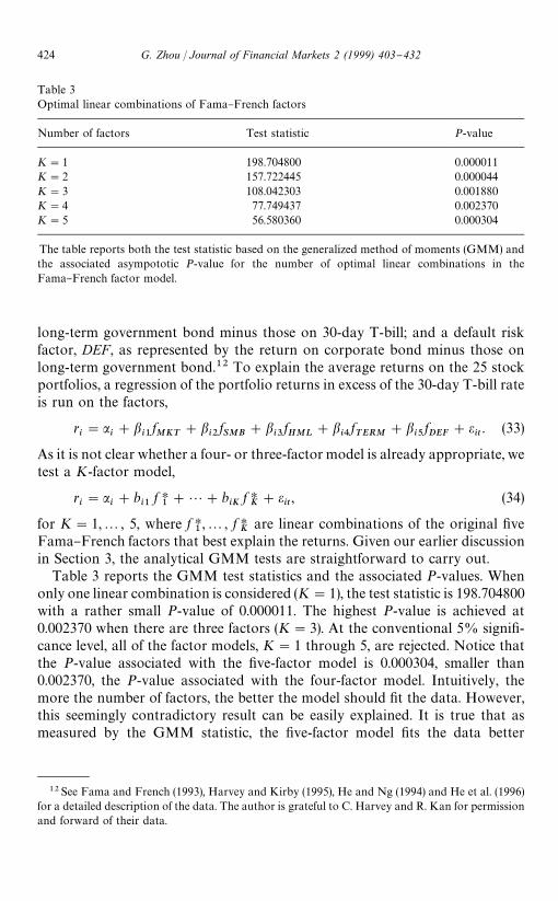
Table 3Optimal linear combinations of Fama}French factors

Number of factors Test statistic P-value

K"1 198.704800 0.000011K"2 157.722445 0.000044K"3 108.042303 0.001880K"4 77.749437 0.002370K"5 56.580360 0.000304

The table reports both the test statistic based on the generalized method of moments (GMM) andthe associated asympototic P-value for the number of optimal linear combinations in theFama}French factor model.

12See Fama and French (1993), Harvey and Kirby (1995), He and Ng (1994) and He et al. (1996)for a detailed description of the data. The author is grateful to C. Harvey and R. Kan for permissionand forward of their data.

long-term government bond minus those on 30-day T-bill; and a default riskfactor, DEF, as represented by the return on corporate bond minus those onlong-term government bond.12 To explain the average returns on the 25 stockportfolios, a regression of the portfolio returns in excess of the 30-day T-bill rateis run on the factors,

ri"a

i#b

i1fMKT

#bi2

fSMB

#bi3

fHML

#bi4

fTERM

#bi5

fDEF

#eit. (33)

As it is not clear whether a four- or three-factor model is already appropriate, wetest a K-factor model,

ri"a

i#b

i1f H1#2#b

iKf HK#e

it, (34)

for K"1,2, 5, where f H1,2, f H

Kare linear combinations of the original "ve

Fama}French factors that best explain the returns. Given our earlier discussionin Section 3, the analytical GMM tests are straightforward to carry out.

Table 3 reports the GMM test statistics and the associated P-values. Whenonly one linear combination is considered (K"1), the test statistic is 198.704800with a rather small P-value of 0.000011. The highest P-value is achieved at0.002370 when there are three factors (K"3). At the conventional 5% signi"-cance level, all of the factor models, K"1 through 5, are rejected. Notice thatthe P-value associated with the "ve-factor model is 0.000304, smaller than0.002370, the P-value associated with the four-factor model. Intuitively, themore the number of factors, the better the model should "t the data. However,this seemingly contradictory result can be easily explained. It is true that asmeasured by the GMM statistic, the "ve-factor model "ts the data better


because it has a statistic of 56.580360, smaller than 77.749437 of the four-factormodel. But the "ve-factor model has 25 additional parameters, and this ispenalized by the test which has now 25 fewer degrees of freedom. In other words,by adding 25 additional parameters, the gain in model "tting cannot o!set theloss in the degrees of freedom of the test, and hence it produces a P-value for the"ve-factor model lower than a four-factor one.

As the number of factors increases from one to "ve, it is of interest to examinehow much contributions each pre-speci"ed factor makes to the linear combina-tion. While the factor loadings provide an answer to this question, they varygreatly as the number of factors changes due to the factor normalization. Hence,a simple approach is to examine the regression coe$cients or weights on each ofthe pre-speci"ed "ve factors. For example, in a one-factor model, the magnitudeof the weight o!ers information on how the original factor contributes to theexplanatory power of the model. In a "ve-factor model, there will be norestrictions on the weights and hence they must be the same as the OLSregression coe$cients from regressing the asset returns on all of the Fama andFrench "ve factors. Table 4 provides the results. This is done only for the 5jthasset ( j"1,2, 5) as results on all of the 25 assets would take too much space.Interestingly, the weights change little as the number of factors varies. Forexample, imposing a one-factor model, the weight or contribution of F

MKTis

1.1864, which is not much di!erent from 1.0711, the weight in the "ve-factormodel. Econometrically, this closeness is likely due to that fact that the one-factor model is designed to have the maximum explanatory power given therestriction on the number of factors. Intuitively, as there is not much change inthe explanatory power from the one-factor model to the "ve-factor one, it is notsurprising that the weights are not too much di!erent.

By the testing results alone, it is di$cult to distinguish among the variousfactor models. Table 5 provides a few model diagnostics that may help shedsome light on the problem. The second column reports the residual errorsaveraged over time and across the assets. The average error tells how the model"ts the data over time and across the assets. The third column reports theabsolute residual errors averaged over time and across the assets. This averageabsolute error detects possibly large and o!setting residual errors. The fourthcolumn reports the average of the R2 across the assets. The in-sample results arecomputed from estimation over the entire sample period. As expected, the morethe number of factors, the better the model "ts the data. From a one-factormodel to a two-factor one, the average error is reduced by about 50%. However,the average errors are almost the same from two- to "ve-factor models. Sim-ilarly, there are not much di!erences in the average absolute errors. In term ofthe R2, it is generally higher with more factors.

As an additional diagnostic, we estimate the models by excluding the last3 years data, and use the newly estimated parameters to compute the R2s for thelast 3 years. This gives rise to the out-of-sample results. In contrast to its


Table 4Weights on the FF factors in the restricted factor model

Number of MKT SMB HML TERM DEFfactors

K"1 1.1864 0.4439 0.3119 !0.0246 !0.05961.1884 0.4446 0.3124 !0.0246 !0.05971.0972 0.4105 0.2885 !0.0228 !0.05511.1135 0.4167 0.2928 !0.0231 !0.05590.8545 0.3197 0.2246 !0.0177 !0.0429

K"2 1.0817 0.7428 0.7534 0.0066 !0.06761.1186 0.6444 0.6011 !0.0058 !0.06701.0482 0.5512 0.4875 !0.0108 !0.06151.0872 0.4934 0.3930 !0.0192 !0.06190.8428 0.3520 0.2608 !0.0180 !0.0473

K"3 1.0551 0.9110 0.6075 !0.0174 !0.12421.1162 0.6588 0.5884 !0.0068 !0.07141.0573 0.4928 0.5378 !0.0010 !0.04131.1104 0.3461 0.5202 0.0037 !0.01170.8906 0.0474 0.5236 0.0303 0.0571

K"4 1.0754 0.8979 0.6222 !0.0643 !0.20591.1234 0.6536 0.5930 !0.0195 !0.09991.0426 0.5015 0.5264 0.0383 0.01801.0981 0.3529 0.5105 0.0394 0.03800.9165 0.0294 0.5402 !0.0182 !0.0465

K"5 1.0711 0.8860 0.6107 0.0374 !0.17961.1233 0.6535 0.5928 !0.0179 !0.09941.0478 0.5154 0.5399 !0.0806 !0.01281.1024 0.3645 0.5217 !0.0596 0.01240.9199 0.0387 0.5492 !0.0979 !0.0671

The table reports the regression coe$cients or weights on each of the pre-speci"ed "ve factors in theK-factor model for the 5jth asset ( j"1,2, 5).

in-sample performance, a "ve-factor performs worse than a two-, three- orfour-factor model as measured by the R2. Combining both the testing and theout-of-sample results, it appears that a three-factor model is better than a "ve-factor one. In other words, there does seem some gain in using a few linearcombinations of the given factors rather than in using all of them.

Our methodology picks up a three-factor model where the factors are linearcombinations of Fama and French's (1993) original "ve. This model performsstatistically better than the "ve-factor model, and also does better (by design)than the three-factor model advocated by Fama and French which simply drops


Table 5Model diagnostics

Number Average Average Averageof factors errors absolute errors R2

In-sample

K"1 !0.000234 0.016741 0.843338K"2 !0.000115 0.015270 0.872199K"3 !0.000104 0.014044 0.894909K"4 !0.000104 0.014004 0.895476K"5 !0.000106 0.013981 0.895440

Out-of-sample

K"1 !0.001458 0.017829 0.776520K"2 !0.001387 0.016923 0.802872K"3 !0.001416 0.016997 0.809803K"4 !0.001438 0.016946 0.804791K"5 !0.001437 0.016967 0.798259

The table reports the average residual errors, the average of the absolute value of the residual errors,and the average (across assets) of the R2. The in-sample results are for the entire sample period, andthe out-of-sample results are for the last three years.

the TERM and DEF factors out of the "ve. However, it remains unknownwhether or not this model can perform better in explaining the cross-section ofexpected stock returns than the Fama and French three-factor model. Toanswer this question, we run the standard OLS two-pass regressions by usingseparately both the extracted factors and those of the Fama and French's chosenthree. The results are summarized in Table 6. The risk premium estimates for theextracted factors are all positive. In contrast, the risk premiums for the threefactors chosen by Fama and French (1993) do not have the same signs. Forexample, Fama and French's estimated market risk premium is !0.0767,slightly negative. As the factors are di!erent, it is di$cult to assess whichthree-factor models is preferred on the basis of the risk premiums (althougha negative market risk premium does not seem plausible from the perspective ofstandard asset pricing theories). Fortunately, the Q

#test statistic is both

a measure of the cross-sectional pricing errors and a test of the asset pricingrestrictions. As Q

#are 0.1226 and 0.1318 respectively, the model with the

extracted factors performs better in explaining the cross-section of expectedstock returns than Fama and French's three-factor one. This is also supportedby the associated p-values, which are 0.01419 and 0.0066, respectively.

Brennan et al. (1998) examine the explanatory power in the cross-section ofstock returns by using 14 economic variables. It seems that the methodology of


Table 6A comparison with Fama and French risk premiums

Q#

c1

c2

c3

Panel A: Risk Premiums for fMKT

, fSMB

and fHML

0.1318 !0.0767 0.1018 0.1797(0.0066) (0.0906) (0.0767) (0.0822)

Panel B: Risk Premiums for f1, f

2and f

3

0.1226 0.1199 0.1463 0.1561(0.0142) (0.2611) (0.2586) (0.2550)

The table reports both the test, Q#, for the asset pricing restrictions (its p-value in the bracket) and

the risk premium estimates (their asymptotic standard errors in brackets) for both the Fama andFrench factors ( f

MKT, f

SMBand f

HML) and the extracted factors ( f

1, f

2and f

3).

this paper can be useful in reducing the number of variables both cross-sectionally and time-series wise. Furthermore, as the variables are from diversesources, it may be of interest to use the extended methodology of Section 2.3 todivide the variables into several groups and to extract the factors from eachgroup accordingly. As the methodology is of the primary interest in this paper,additional empirical applications appear to go beyond the scope of this paper.

6. Conclusions

This paper provides a new framework to extract factors from either a latentfactor model or a factor model with pre-speci"ed factors. In particular, itpresents a useful technique to "nd linear combinations of known economicvariables that best forecast latent factors, such as those in Ross's (1976) arbitragepricing theory and those in models of the term structure of interest rates. Basedon the proposed model, we provide a test for the APT based on the generalizedmethod of moments (GMM). This test is potentially more robust than almost allof the existing ones because it does not su!er from the usual errors-in-variablesproblem, nor does it require the strong assumption that the security returns arenormally distributed and temporarily independent.

By using monthly industry returns and the "ve economic variables of Chenet al. (1986), we "nd that a two-factor APT model cannot be rejected: a linearcombination of industrial production and change in expected in#ation deter-mines the "rst factor and a linear combination of default risk and term premiumdetermines the second. The methodology of the paper appears generallyuseful in identifying from commonly used or collected economic variables the


underlying factors that a!ect security returns and the term structure of interestrates. As an application of extracting factors as linear combinations of pre-speci"ed factors, we extract and test whether fewer factors out of the "ve of Famaand French (1993) are su$cient to explain the average returns on their 25 stockportfolios formed on size and book-to-market. While inconclusive in sample,a three-factor model appears to perform better out-of-sample than both four- and"ve-factor models. It seems interesting future research to apply the methodologyof this paper to extract factors for international security returns and for the termstructure of interest rates where parsimony in the number of factors is veryimportant for pricing bonds and other interest rate derivative securities.

Appendix A. Derivatives of the objective function

For the reader's convenience, this appendix provides an explicit expression forD

Tthat is useful for implementing computations of the analytical GMM test as

well as for checking possible coding errors by examining whether D@T

WTuT

iszero.

Consider "rst the case where a is constrained to zero. In this case, we canorder the normalized h as h"(C

11,2,C

M1,2, C

1K,2, C

MK, A

(K`1)1,2,

A(K`1)K

,2,AN1

,2, ANK

). Writing out Ut

in terms of the parameters andobservables, we obtain the expression

DT"

1

¹

T+t/1

LUt

Lh?Z

t,

1

¹

T+t/1

C!U

10

!U3

!U4D?Z

t, (A.1)

where U1

is a K]KM submatrix, U3

is a (N!K)]KM submatrix, and U4

is(N!K)](q!KM) submatrix of the N]q matrix of partials of U

twith respect

to the parameters. The submatrices can be written

U1"C

Xt1

2 XtM

) 2 ) 0 2 0

F 2 F F 2 F F 2 F

0 2 0 0 2 0 Xt1

2 XtMD , (A.2)

U3"C

A(K`1)1

Xt1

2 A(K`1)1

XtM

) 2 ) A(K`1)K

Xt1

2 A(K`1)K

XtM

F 2 F F 2 F F 2 F

AN1

Xt1

2 AN1

XtM

) 2 ) ANK

Xt1

2 ANK

XtM

D ,

and

U4"C

+Cj1

Xtj

2 +CjK

Xtj

) 2 ) 0 2 0

F 2 F F 2 F F 2 F

0 2 0 ) 2 ) +Cj1

Xtj

2 +CjK

XtjD .


Consider now the case where a is unconstrained. There are N more parametersand h"(a@,C

11,2,C

M1,2,C

1K,2,C

MK,A

(K`1)1,2,A

(K`1)K,2,A

N1,2,

ANK

). It is clear that we need only to add !IN

into the previous LUt/Lh matrix

to compute DT.

Appendix B. Analytical iterations

To show (15), we re-write the model as

Rt"a#A

1C1

Xt1#2#A

pCpXtp#U

t(B.1)

"[a, A1,2, A

p]A

1

C1

Xt1

F

CpXtpB#U

t. (B.2)

Denote the "rst term of Eq. (B.2) as AXt. Using the matrix formula,

vec(PAQ)"(Q@?P)vecA, on the vec operator sucessively, we obtain

AXt?Z

t"vec[Z

t) 1 ) (AX

t)@]

"vec(ZtX @

tA@I

N)"(I

N?Z

tX @

t)vecA@. (B.3)

Hence, the GMM sample moments function has the following form:

gT"

1

¹

T+t/1

(Rt!AX

t)?Z

t"y!XHHa, (B.4)

where y, XHH and a are the same as those de"ned in the text. It then follows from(B.4) that (15) holds as the solution to the GMM minimization problem.

To show (16), we re-write the model as

Rt"a#(X @

1?A

1)vecC

1#2#(X @

p?A

p)vecC

p#U

t(B.5)

"a#[X @1?A

1, 2, X @

p?A

p]A

vecC1

F

vecCpB#U

t. (B.6)

Denote the "rst two terms of Eq. (B.6) as a#XItC. Now, it is easy to show that

XItC?Z

t"(XI

t?Z

t)vec C@ and hence we have (16).

References

Bakshi, G.S., Chen, Z., 1996. Asset pricing without consumption or market portfolio data. Workingpaper, Ohio State University.


Breeden, D.T., Gibbons, M.R., Litzenberger, R.H., 1989. Empirical tests of the consumption basedCAPM.. Journal of Finance 44, 231}262.

Brennan, M.J., Chordia, T., Subrahmanyam, A., 1998. Cross-sectional determinants of expectedreturns. Journal of Financial Economics 49, 345}373.

Brown, S.J., Goetzmann, W.N., Grinblatt, M., 1997. Positive portfolio factors. Working paper, YaleUniversity.

Chen, N.-f., Roll, R., Ross, S.A., 1986. Economic forces and the stock market. Journal of Business 59,383}403.

Connor, G., 1984. A united beta pricing theory. Journal of Economic Theory 34, 13}31.Connor, G., Korajczyk, R.A., 1986. Performance measurement with the arbitrage pricing theory:

A new framework for analysis. Journal of Financial Economics 15, 373}394.Connor, G., Korajczyk, R.A., 1995. The arbitrage pricing theory and multifactor models of asset

returns. in: Jarrow, R.A. (Ed.), Handbooks in Operations Research and Management Science:Finance, Vol. 9. North-Holland, Amsterdam, pp. 87}144.

Epps, T.W., Kramer, C.F., 1995. A variance test of the linear factor representation of returns andequilibrium pricing restrictions. Working paper, University of Virginia.

Fama, E.F., French, K.R., 1993. Common risk factors in the returns on stocks and bonds. Journal ofFinancial Economics 33, 3}56.

Ferson, W.E., Harvey, C.R., 1991. The variation of economic risk premiums. Journal of PoliticalEconomy 99, 385}415.

Geweke, J., Zhou, G., 1996. Measuring the pricing error of the arbitrage pricing theory. Review ofFinancial Studies 9, 553}583.

Gibbons, M.R., Ferson, W., 1985. Testing asset pricing models with changing expectations and anunobservable market portfolio. Journal of Financial Economics 14, 217}236.

Gibbons, M.R., Ross, S.A., Shanken, J., 1989. A test of the e$ciency of a given portfolio. Econo-metrica 57, 1121}1152.

Hansen, L.P., 1982. Large sample properties of the generalized method of moments estimators.Econometrica 50, 1029}1054.

Hansen, L.P., Jagannathan, R., 1997. Assessing speci"cation errors in stochastic discount factormodel. Journal of Finance 52, 557}590.

Harvey, C.R., Kirby, C., 1995. Analytic tests of factor pricing models. Working paper, DukeUniversity, Durham, NC.

He, J., Ng, L.K., 1994. Economic forces, fundamental variables, and equity returns. Journal ofBusiness 67, 599}609.

He, J., Kan, R., Ng, L.K., Zhang, C., 1996. Tests of the relationships among economic forces,fundamental variables, and equity returns using multi-factor models. Journal of Finance 51,1891}1908.

Ingersoll, J.E., 1987. Theory of Financial Decision Making. Rowman and Little"eld, New York.Jagannathan, R., Wang, Z., 1996. The conditional CAPM and the cross-section of expected returns.

Journal of Finance 51, 3}53.JoK reskog, K.G., Goldberger, A.S., 1975. Estimation of a model with multiple indicators and

multiple causes of a single latent variable. Journal of American Statistical Association 70,631}639.

Lehmann, B.N., Modest, D.M., 1988. The empirical foundations of the arbitrage pricing theory.Journal of Financial Economics 21, 213}254.

Lintner, J., 1965. The valuation of risk assets and the selection of risky investments in stockportfolios and capital budgets. Review of Economics and Statistics 47, 13}37.

MacKinlay, A.C., Richardson, M.P., 1991. Using generalized method of moments to test mean-variance e$ciency. Journal of Finance 46, 511}527.

Nardari, F., Zhou, G., 1999. What is the decomposition of the market wealth portfolio in theCAPM? Working paper, Washington University.


Newey, W.K., 1985. Generalized method of moments speci"cation testing. Journal of Econometrics29, 229}256.

Newey, W.K., West, K.D., 1987. A simple, positive semi-de"nite, heteroskedasticity and autocorrela-tion consistent covariance matrix. Econometrica 55, 703}708.

Roll, R., 1977. A critique of the asset pricing theory's tests: Part I. Journal of Financial Economics 4,129}176.

Ross, S.A., 1976. The arbitrage theory of capital asset pricing. Journal of Economic Theory 13,341}360.

Seber, G.A.F., 1984. Multivariate Observations. Wiley, New York.Shanken, J., 1985. Multivariate tests of the zero-beta CAPM. Journal of Financial Economics 14,

327}348.Shanken, J., 1992. The current state of the arbitrage pricing theory. Journal of Finance 47,

1569}1574.Shanken, J., 1996. Statistical methods in tests of portfolio e$ciency: a synthesis. in: Maddala, G.S.,

Rao, C.R. (Eds.), Handbooks of Statistics: Statistical Methods in Finance, Vol. 14. North-Holland, Amsterdam, pp. 693}711.

Sharpe, W.F., 1964. Capital asset prices: A theory of market equilibrium under conditions of risk.Journal of Finance 19, 425}442.

Stambaugh, R., 1982. On the exclusion of assets from tests of the two-parameter model: a sensitivityanalysis. Journal of Financial Economics 10, 237}268.

Velu, R., Zhou, G., 1999. Testing multi-beta pricing models. Journal of Empirical Finance, forthcom-ing.

Zhou, G., 1994. Analytical GMM tests: asset pricing with time-varying risk premiums. Review ofFinancial Studies 7, 687}709.


security factors as linear combinations of economic...

Documents