Sediment Properties Sediment Properties Determined through Determined through

MagnetotelluricsMagnetotelluricsBy: Andrew Frassetto

University of South Carolina

July 17, 2002

Outline:Outline:•Overview of field area•The Magnetotelluric Method•Examples of MT Curves and 1-D Inversion Models•Description of the Geoelectric profile•My focus: Determining sediment properties of shallow, low resistivity layer•Problems in determining sediment properties using Archie’s Law (and Wyllie’s Equation)•Summary of results and interpretations regarding porosity and seismic velocity•Implications of the sediment properties

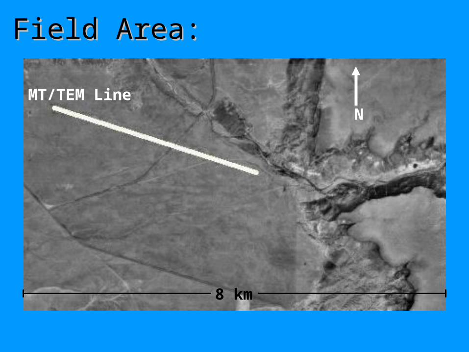
Field Area:Field Area:

MT/TEM Line N

8 km

The Basics of The Basics of MT:MT:•Low frequency, passive, deep imaging of the

Earth’s lithosphere•Traditionally uses Ex and Ey, along with Hx, Hy, Hz (Titan-24 System did not measure Hz)

(Jiracek et al., 1995)

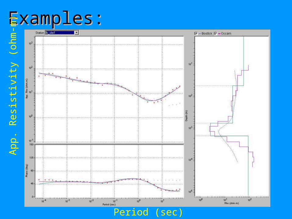
MT at SAGE MT at SAGE 2002:2002:•On an MT curve, a

positive slope indicates a resistive layer, while a negative slope shows increasing conductivity. The increasing period represents a lowering frequency at depth.

(Jiracek et al., 1995)

•SAGE 2002’s MT setup consisted of 41 separateData collection points spread at 100 m intervals over 4.1 km. The data was collected in 2 days.

Examples:Examples:A

pp.

Res

istiv

ity (

ohm

-m)

Period (sec)

Examples:Examples:A

pp.

Res

istiv

ity (

ohm

-m)

Period (sec)

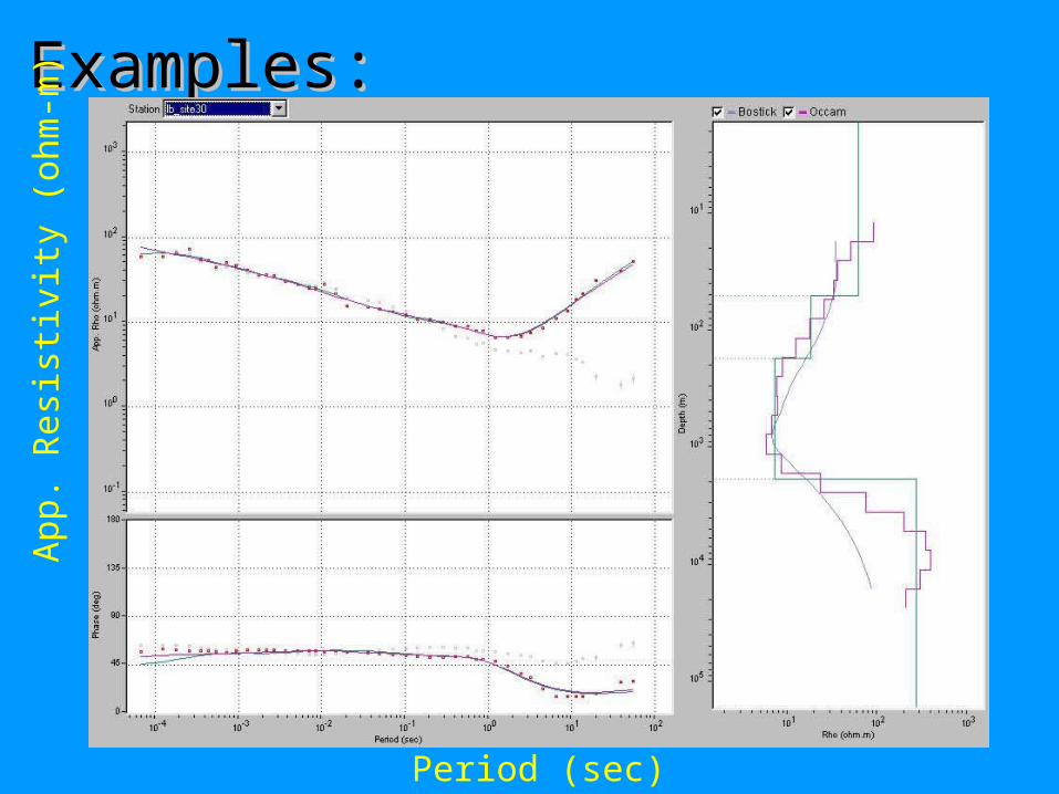
Examples:Examples:

Period (sec)

App

. R

esis

tivity

(oh

m-m

)

Examples:Examples:A

pp.

Res

istiv

ity (

ohm

-m)

Period (sec)

Initial Initial Observations:Observations:•From the 1-D Inversion model, 4 basic layers can

be seen: -a thin resistive surface layer -a 150-650 m thick layer of low resistivity -a 1000-1500 m thick layer of high conductivity -the highly resistive basement at 2500-3500 m

•The basement layer becomes shallower down the line, with the conductive layer becoming thinner

•The subsequent 1-D Inversion stitch illustrates these layers fairly well

Geoelectric Geoelectric Profiles:Profiles:

Precambrian Basement: 2.5-3.5 km depth

Area of Focus

De

pth

(m

)

Distance (km)

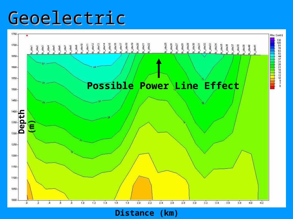
Geoelectric Geoelectric Profiles:Profiles:

Possible Power Line Effect

De

pth

(m

)

Distance (km)

Well Data:Well Data:

Flora Barres Well

Data from a geochemical analysis was used to estimate the resistivity of water in this region using a Salinity-Porosity Nomogram. Thus, porosity can be calculated using Archie’s Law.

(Longmire, 1985)

Calculations:Calculations:

The well data include temperature (18.1 ˚C) and equivalent salinity (385 ppm). Plotting these on the Nomogram and connecting them with a best fit line yields ρw ≈ 14 ohm-

m.

(SAGE 2002 Notes)

Calculations - Porosity:Calculations - Porosity:Archie’s Law: ρr / ρw = aΦ-m …where a is the

coefficient of saturation and m is the cementation factor. ρr was taken from the 1-D inversion model

Values range from 8 ohm-m to 34 ohm-m, with most approximately 20 ohm-m.

Humble Formula: a = 0.62, m = 2.15…used in sandstone environments and this study

Archie’s Law cannot be applied to clay environments, as clay drastically increases the conductivity and renders porosity estimates useless.

Calculations – Seismic Calculations – Seismic Velocity:Velocity:Wyllie’s Equation:

1/v = Φ/vf + 1-Φ/vm

…where vf is the velocity of the fluid and vm is the velocity of the matrix rock, in this case assumed to be granite. As such, vf = 1510 m/s and vm = 5375 m/s.

Data:Data:

Calculated Results: Φ ≈ 29% vp = 3148.28 m/s

(SAGE 2002 Notes)

Several data points were dropped due to power lines in center and clays near the end of MT line.

Graphs:Graphs:

Graphs:Graphs:

Interpretations:Interpretations:

Φ ≈ 25-35%: potential aquifer Possible clay zone

Significant clay & possible increase in salinity?: poor aquifer

Conclusions:Conclusions:•Resistivities are a reasonable method to estimate the porosity of buried sediments or rocks.

•Calculated values for porosity and sand maintain fairly consistent across the profile.

•The values suggest a large amounts of loosely consolidated, non-lithified sand to a depth of 660 m.

•This region of basin has low the potential to be an excellent freshwater aquifer.

References:References:Jiracek, G.R., Haak, V., Olsen, K.H., 1995, Practical magnetotellurics in a continental rift environment. In: K.H. Olsen (ed.), Continental Rifts: Evolution, Structure, and Tectonics, Developments in Geotectonics Vol. 25, Elsevier, Amsterdam, p. 103-128

Longmire, P., 1985, A Hydrogeochemical Study Along the Valley of the Santa Fe River, Santa Fe and Sandoval Counties, New Mexico. Ground Water and Hazardous Waste Bureau, Santa Fe, p. 01-35

Ward, S.H., 1990, Resistivity and induced polarization methods. In: Ward, S.H. (ed.), Geotechnical and environmental geophysics, Vol. 1, Society of Exploration Geophysicists, p. 147-189

SAGE 2002 Handbook

AcknowledgemeAcknowledgements:nts:•Quantec and Zonge Engineering for their

equipment and expertise

•Cochiti Pueblo for allowing us the privilege of working on their land

•David and George for always taking the time to answer one of my many questions

•Lauren for the TEM data, through which all static shift corrections were possible

•The entire SAGE 2002 group for making this such a great experience