seeking a seaﬂoor magnetic signal from the antarctic

March 26, 2004 20:22 Geophysical Journal International gji2174

Geophys. J. Int. (2004) 157, 175–186 doi: 10.1111/j.1365-246X.2004.02174.x

GJI

Mar

ine

geos

cien

ce

Seeking a seafloor magnetic signal from the Antarcticcircumpolar current

F. E. M. Lilley,1 A. White,2 G. S. Heinson3 and K. Procko4

1Research School of Earth Sciences, Australian National University, Canberra, ACT 0200, Australia. E-mail: [email protected] of Chemistry, Physics and Earth Sciences, Flinders University, Adelaide, SA 5001, Australia. E-mail: [email protected] of Earth and Environmental Sciences, University of Adelaide, Adelaide, SA 5005, Australia. E-mail: [email protected] School of Earth Sciences, Australian National University, Canberra, ACT 0200, Australia. E-mail: [email protected]

Accepted 2003 October 23. Received 2003 October 6; in original form 2002 December 11

S U M M A R YMotional electromagnetic induction by ocean currents is a basic phenomenon of geophysics,with application to the monitoring of ocean transport. One of Earth’s strongest ocean currents isthe Antarctic circumpolar current (ACC). This paper explores the magnetic signals that shouldbe generated by the ACC, and reports an experiment in which a magnetometer recorded naturalvariations of Earth’s magnetic field on the floor of the Southern ocean for some five monthsin 1996. Magnetometer records from Kingston, Tasmania, and from Macquarie Island givereference information concerning magnetic storms and substorms. The instrument was sited inthe region of the major oceanographic subantarctic flux and dynamics experiment (SAFDE),where the ACC passes south of Tasmania, between the major topographic features of theSouth Tasman rise and the Australia–Antarctica spreading ridge. The SAFDE records givecomprehensive control on the actual ocean current flow at the time of the magnetic recording,and allow a magnetic signal to be predicted, in terms of the seafloor conductance. The seafloorconductance for the area is however low, and the amplitude of the predicted signal is low. Theseafloor observations confirm that the signal is weak against the effects of ionospheric signals.In future experiments, the choice of sites with thicker seafloor sedimentation would increasethe ACC magnetic signal to be observed.

The magnetometer measurements have a result relevant for the SAFDE, in confirming thatthe correction of electric data for seafloor conductance is small. There is also the result forseafloor magnetic observatories for which motional induction effects are unwanted, that suchan observatory can operate even under the ACC, and be substantially protected from motionalinduction effects by low seafloor conductance.

Key words: Antarctic, geomagnetism, circumpolar current, motional induction, seafloormagnetometers, Southern ocean.

1 I N T RO D U C T I O N

The global network of magnetic observatories has grown steadilysince the first international network was established in the 19th cen-tury by Ross (Barraclough et al. 1992). The present situation for theAustralian region is reviewed by Hopgood (2001).

Only in the last twenty or thirty years have seafloor observatoriesbecome a possibility, and much attention is being given at present tothe challenge of complementing the network of land observatorieswith others on the seafloor (Chave et al. 1995; Toh & Hamano 1997).This task is especially significant as some two-thirds of the Earth iscovered by ocean.

In the present experiment, four seafloor instruments were de-ployed on the floor of the Southern ocean in 1996 April. Two were

recovered a year later in 1997, and two in 1998. The intentions ofthe experiment were several:

(i) To establish the feasibility of deployment and recovery of themagnetometer package in the hostile environment of the Southernocean.

(ii) To make initial seafloor measurements in the latitude of theSouthern auroral zone.

(iii) to analyse the fluctuation data for ocean-floor conductivitystructure in the vicinity of the Antarctic–Australia spreading ridge.

(iv) To examine the data for evidence of a magnetic signal causedby the motional induction of the Antarctic circumpolar current, espe-cially in the context of a major experiment in physical oceanographytaking place there at that time.

C© 2004 RAS 175


176 F. E. M. Lilley et al.

x

yz

SEA SURFACEz = 0

SEA FLOORz = -HSEDIMENTS

z = -H-h

Bv x B E J

v b

RETURN J

leakage J

σ1

σ2

σ= 0

Figure 1. Figure for theory of motional induction.

Of the four instruments deployed, two failed to record any data, andof the two instruments which did record data, just one functionedcorrectly. The records from this instrument form the basis of thispaper, which addresses particularly the fourth of the objectives listedabove.

To provide simultaneous magnetic records for reference purposes,a land station was operated at Kingston, Tasmania. This site is tothe north of the seafloor sites. Also the magnetic observatory atMacquarie Island, to the southeast of the seafloor sites, providedsimultaneous reference data.

The seafloor observations were planned to coincide with a majoroceanographic experiment, the subantarctic flux and dynamics ex-periment (SAFDE) of Luther et al. (1997). This experiment, part ofthe larger world ocean circulation experiment (WOCE), thoroughlyinstrumented the ACC south of Tasmania for two years, 1995–1996.The results of the SAFDE provide valuable information for assess-ing the results of the present magnetometer experiment.

Initially in setting a time base for the magnetometer data, elapseddays (or edays) have been defined, as the elapsed time since the start

0 5 10 15 20 25 30 35 40 45 500

5

10

15

20

25

30

35

40

45MOTIONAL INDUCTION BY SOUTHERN OCEAN CURRENTS

CHANGE IN SANFORD VELOCITY (cm s−1)

CH

AN

GE

IN S

EA

FLO

OR

MA

GN

ET

IC S

IGN

AL

(nT

)

10 S50 S

100 S

200 S

400 S

600 S

800 S

1000 S

Figure 2. Change in seafloor magnetic signal, in terms of change in the Sanford velocity (v∗), for different values of seafloor conductance as marked insiemens (S).

of 1996 January 1 reckoned in units of days. Then, for consistencywith the SAFDE data, the SAFDE convention is adopted of definingdigital days as those elapsed since the start of 1995 January 1. A1995 elapsed day value is obtained from a 1996 elapsed day valueby the addition of 365. Thus 06.00 h on 1996 January 2 UT wouldhave a 1996 elapsed day value of 1.25, and a 1995 elapsed day valueof 366.25.

2 T H E O RY

The theory for seafloor magnetic fields generated by ocean currentsis as developed by Sanford (1971), following Longuet-Higgins et al.(1954). There are relevant papers by Chave & Luther (1990) andLarsen (1992). The notation adopted here follows the descriptionin Lilley et al. (1993), where examples of seafloor magnetic fieldgenerated by the east Australian current (EAC) are reported. Themeasurement of motional magnetic fields down through the oceancolumn in the EAC is described by Lilley et al. (2001).

The physical circumstances are as in Fig. 1. The sea water haselectrical conductivity σ 1, and is underlain by a sedimentary layerof conductivity σ 2, below which the conductivity is taken as zero.The ocean velocity is in the y direction, and varies with z only.Denoting the ocean velocity by vy(z), the electric current flow byJx(z), the electric field by Ex, the steady vertical magnetic fieldby Bz, the perturbation magnetic field due to motional induction byby(z), and the local electrical conductivity by σ (z), then Ohm’s lawfor a moving medium may be expressed as

Jx (z) = σ (z)[Ex + vy(z)Bz]. (1)

For the present paper, an important result is that the seafloormagnetic field, bs, can be expressed as

bs = −µ0σ2 h Ex , (2)

and, using notation v∗ for (−Ex/Bz),

bs = µ0σ2h Bzv∗, (3)

C© 2004 RAS, GJI, 157, 175–186


Seafloor magnetometers 177

where v∗ is Sanford’s vertically-averaged and sea waterconductivity-weighted water velocity:

v∗ =∫ 0

−Hσ (z)vy(z) dz

/ ∫ 0

−H−hσ (z) dz. (4)

The seafloor perturbation magnetic field bs is thus: directly pro-portional to Bz, the vertical component of the ambient main magneticfield; approximately proportional to the seafloor conductance σ 2h(this quantity also enters weakly into v∗); and, for constant σ 2h, di-rectly proportional to the Sanford velocity as represented by v∗. Forthe site Girardin (introduced below) the value of µ0 Bz is −8.14 ×10−11 SI units, and, ignoring the negative sign, the relationship ofeq. (3) may be expressed as in Fig. 2.

Note that seafloor magnetic data will generally be relative to anunknown zero. This circumstance prevails because the strength ofthe magnetic field at the seafloor, in the absence of any motionalinduction contribution, cannot be predicted with sufficient accuracy(and measurements may involve an unknown induction contribu-tion). Seafloor magnetic data may therefore contain informationabout variation in a motional induction signal, but not its steadyvalue. For this reason, Fig. 2 is plotted in terms of changes in San-ford velocity and seafloor magnetic field. With reference to Fig. 2,for a seafloor conductance of 400 S, a change in the Sanford velocityof the ACC corresponding to 30 cm s−1 will give a change in seafloormagnetic signal of order 10 nT. For a lesser seafloor conductanceof 40 S, the seafloor magnetic signal is reduced to 1 nT. Seafloorconductance is thus critical in the observation of motional magneticsignals on the seafloor. For the case reported by Lilley et al. (1993),the Tasman abyssal plain off the east coast of Australia has a seafloorsediment thickness of order 1 km, giving a seafloor conductance ofsome 800 S.

Observations in the latitudes of the ACC carry the benefit thatthe vertical component of Earth’s magnetic field, Bz, which enterseq. (3) above, is close to its maximum strength for the Earth. Thereis the disadvantage, at such latitudes, that magnetic storms and othersignals arising in the ionosphere outside the solid Earth are intense,due to the presence of the auroral zone (Campbell 1997). Distin-guishing a signal of oceanic origin from one of ionospheric originmay be expected to depend, first, on exploiting differences in fre-quency content between the two: the oceanic signals sought shouldbe of longer timescale than the ionospheric signals. Secondly, dif-ferences in horizontal length-scale may be exploited, as generally anionospheric disturbance should be coherent over a greater horizontaldistance than an oceanic feature such as an eddy.

A further relevant point for the Southern ocean, made by Chave &Luther (1990), is that the vertical variation of electrical conductivityin the ocean column is weak. As a result, in eq. (4), first, the Sanfordvelocity becomes very nearly the vertically-averaged ocean velocity,with a coefficient dependent on the seafloor conductance. Secondly,if the seafloor conductance is small, the Sanford velocity becomesvery nearly, simply the vertically-averaged ocean velocity.

An extra factor in the present case arises with the availability ofreference data from the Macquarie Island magnetic observatory. Ac-cording to the basic theory, such a surface observatory should detectno magnetic signal due to motional induction by sea water. Thus inthe analysis below, the Macquarie Island data, after smoothing, willbe compared directly with the seafloor data. It is well known thatmagnetic storm activity at the seafloor will be an attenuated ver-sion of what is seen at the surface (due to the attenuating effect ofpropagation down through the ocean water). However, the sea waterattenuating effect is frequency dependent, and will be negligible for

Table 1. Details of deployment sites (number, name, code, latitude, lon-gitude, ocean depth) of magnetometers in the SOMEx. Details for the landreference sites are also given. The seafloor names record personnel of theD’Entrecasteaux expedition of 1791–1793, which made magnetic measure-ments in southern Tasmania in 1792, (De Rossel 1808)).

Seafloor1 Bruny BRN 48◦42′S 144◦44′E 3860 mSeafloor2 Huon HUO 49◦49′S 144◦14′E 3700 mSeafloor3 Rossel ROS 50◦38′S 143◦49′E 3605 mSeafloor4 Girardin GIR 51◦45′S 143◦17′E 3500 mLand Kingston KIN 43◦00′S 147◦18′E SurfaceObsrvtry Macquarie MCQ 54◦30′S 158◦57′E Surface

periods of several days and longer, which is the period band of theocean current phenomena of interest.

3 S E A F L O O R I N S T RU M E N TAT I O NA N D O B S E RVAT I O N S I T E S

The seafloor instruments used were three-component fluxgate mag-netometers, as developed at Flinders University of South Australia,Adelaide. The origins of these instruments lie in designs describedby White (1979) and Chamalaun & Walker (1982). With vari-ous successive improvements, the instruments have been used torecord seafloor data in a range of experiments, such as EMSLAB-Group (1988) and White & Heinson (1994). For the Southern ocean

Figure 3. Map showing the magnetometer sites and bathymetry (m).

C© 2004 RAS, GJI, 157, 175–186



magnetometer experiment (SOMEx) deployments each magne-tometer was packed into the space available inside a standardacoustic-release glass sphere, without compromising the acousticrelease facility. The spheres were of diameter 17 in (0.43 m), thusmaking a compact instrument for deep-ocean marine studies. Forthe SOMEx deployments, the replacement of the earlier linear flux-gate sensors with newly-developed ring core fluxgate sensors was arecent design improvement.

The magnetometers were set to record at a data interval of 60s, and so (with the memory capacity of that time) could recordfor six months. Deployed in 1996 April from the Antarctic vesselAurora Australis during its Voyage 6 of 1995–96, they were alloweda mechanical and thermal stabilisation period of two months, andthen were set to commence recording at 00.00 h on 1996 June 1 UT.

During deployment the instruments are released from the de-ploying vessel, and free-fall to the ocean floor, at a descent rate ofapproximately 1 m s−1. On the seafloor the orientation in which amagnetometer settles is recorded and recovered by the three com-

500 520 540 560 580 600 620 640 660 680 700−1.24−1.22

−1.2

x 104

xb (

nT)

SOMEx 96: data 7A280398.lrt

500 520 540 560 580 600 620 640 660 680 700500

10001500

yb (

nT)

500 520 540 560 580 600 620 640 660 680 700−6.36

−6.34

x 104

zb (

nT)

500 520 540 560 580 600 620 640 660 680 7006.44

6.46

6.48x 10

4

F (

nT)

500 520 540 560 580 600 620 640 660 680 7001.35

1.4

x 104

x (n

T)

500 520 540 560 580 600 620 640 660 680 700

4050410041504200

y (n

T)

500 520 540 560 580 600 620 640 660 680 700−6.32

−6.3

−6.28x 10

4

z (n

T)

500 520 540 560 580 600 620 640 660 680 700

1.421.441.461.48

x 104

fh (

nT)

500 520 540 560 580 600 620 640 660 680 700

−0.5−0.4−0.3

X–l

ev (

deg)

500 520 540 560 580 600 620 640 660 680 7006.46.66.8

77.2

Y–l

ev (

deg)

500 520 540 560 580 600 620 640 660 680 700−0.4

−0.2

deg.

C

500 520 540 560 580 600 620 640 660 680 7006.26.46.66.877.2

Vol

t

500 520 540 560 580 600 620 640 660 680 700

143143.5

144

rotn

(dg

)

elapsed days 1995

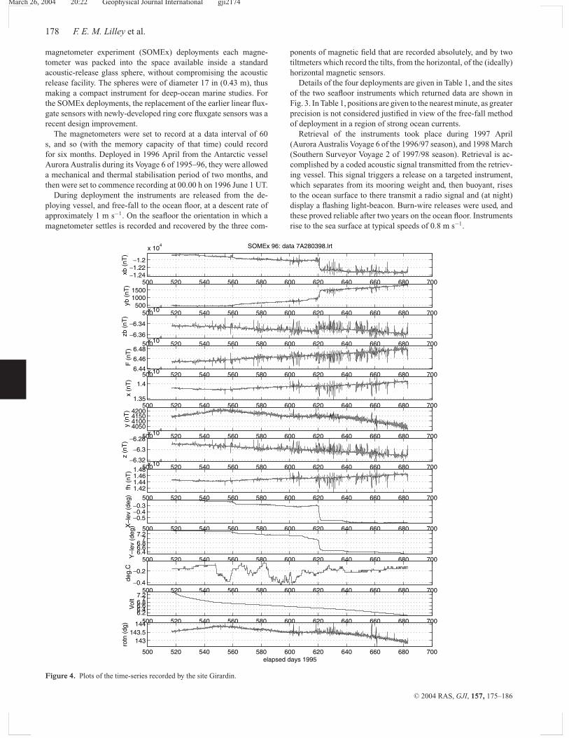
Figure 4. Plots of the time-series recorded by the site Girardin.

ponents of magnetic field that are recorded absolutely, and by twotiltmeters which record the tilts, from the horizontal, of the (ideally)horizontal magnetic sensors.

Details of the four deployments are given in Table 1, and the sitesof the two seafloor instruments which returned data are shown inFig. 3. In Table 1, positions are given to the nearest minute, as greaterprecision is not considered justified in view of the free-fall methodof deployment in a region of strong ocean currents.

Retrieval of the instruments took place during 1997 April(Aurora Australis Voyage 6 of the 1996/97 season), and 1998 March(Southern Surveyor Voyage 2 of 1997/98 season). Retrieval is ac-complished by a coded acoustic signal transmitted from the retriev-ing vessel. This signal triggers a release on a targeted instrument,which separates from its mooring weight and, then buoyant, risesto the ocean surface to there transmit a radio signal and (at night)display a flashing light-beacon. Burn-wire releases were used, andthese proved reliable after two years on the ocean floor. Instrumentsrise to the sea surface at typical speeds of 0.8 m s−1.

C© 2004 RAS, GJI, 157, 175–186



4 DATA R E C O R D E D

4.1 Girardin

As a demonstration of the circumstances of seafloor recording, andthe process of data reduction, the records from station Girardin overfive months, and derived time-series, are shown in compressed formin Fig. 4.

The top three traces show the signals recorded by the three mag-netometer sensors on the seafloor. The next trace, F, is a total fieldsignal computed from the upper three. The next three traces, X, Yand Z, are the geographic north, east, and downwards componentsrespectively, obtained by levelling the observed traces according tothe tilt records (X-lev and Y-lev, ninth and tenth traces), and thenrotating the axes of observation horizontally so that X is in the di-rection of geographic north at the start of the observing period. Thetilt calibrations applied have been for an ambient temperature of

500 520 540 560 580 600 620 640 660 680 700

3800

4000

xb (

nT)

SOMEx 96: data 7D280398.lrt

500 520 540 560 580 600 620 640 660 680 700

630064006500

yb (

nT)

500 520 540 560 580 600 620 640 660 680 700−6.44

−6.42

−6.4x 10

4

zb (

nT)

500 520 540 560 580 600 620 640 660 680 700

6.46

6.48

x 104

F (

nT)

500 520 540 560 580 600 620 640 660 680 700920094009600

x (n

T)

500 520 540 560 580 600 620 640 660 680 700260027002800

y (n

T)

500 520 540 560 580 600 620 640 660 680 700

−6.4

−6.38

x 104

z (n

T)

500 520 540 560 580 600 620 640 660 680 70096009800

10000

fh (

nT)

500 520 540 560 580 600 620 640 660 680 7009

9.5

10

X–

lev

(deg

)

500 520 540 560 580 600 620 640 660 680 700−13.4−13.2

−13−12.8−12.6−12.4

Y–

lev

(deg

)

500 520 540 560 580 600 620 640 660 680 700−0.5−0.4−0.3

deg.

C

500 520 540 560 580 600 620 640 660 680 7006.26.46.66.877.27.4

Vol

t

500 520 540 560 580 600 620 640 660 680 700

−130−129.5

−129

rotn

(dg

)

elapsed days 1995

Figure 5. Plots of the time-series (edited) recorded by the site Rossel. Some remaining noise spikes are evident.

zero degrees. The eighth trace, fh, is the horizontal component inthe direction of magnetic north.

The lower three traces are the temperature recorded in the mag-netometer (readings were taken every 156 min), the voltage sup-ply (steadily decreasing, in accordance with correct operation), and(bottom trace) the angle for rotation of the axes to magnetic north(which corresponds to the value of the Y trace, sixth trace down).

It can be seen that Girardin changed orientation slowly, exceptfor a shift at day 620. It experienced some changing temperatureconditions from day 550 to 630, of amplitude some half-degreecentigrade.

The design of the magnetometers incorporates voltage regula-tion to counter the effect of weakening batteries, and so reduce theeffects of drift that a weakening power supply might cause. The de-ployments in the SOMEx produced the longest records yet observedby the magnetometers. In Fig. 4 it is therefore difficult to judgewhat is instrumental drift and what might be true long-period signal.

C© 2004 RAS, GJI, 157, 175–186



Extra information comes from the independent instrument at Rossel,discussed in the next section.

4.2 Rossel

Records from station Rossel over five months, and derived time-series, are shown in compressed form in Fig. 5.

The station Rossel, however, incurred intermittent faults. Whileediting many obvious spikes in the magnetic time-series has reducedthe impact of these faults, the Rossel time-series is generally judgedto be unsuitable for seeking small changes of long timescale. Thereare, however, some periods for which the Rossel time-series is errorfree. One such day from Rossel is included below in Fig. 6, whichshows plots of data from four stations.

The long-term drifts of the Rossel sensors may be compared withthose of Girardin, to look for consistency due to real secular change.Generally the drifts are too great, and too inconsistent between thetwo instruments, to expect them to be real. For example, the in-ternational geomagnetic reference field (IGRF) model predicts asecular change of −14 nT yr−1 in the total field, F, at Girardin andRossel, while Figs 4 and 5 indicate changes of hundreds of nT yr−1

(positively).This behaviour of the seafloor instruments emphasizes the strin-

gent stability required for seafloor observation over long periods.The seafloor environment is stable regarding temperature, as shownby the temperature data in Figs 4 and 5. However, from the start

630 630.5 6311.6

1.65

1.7

x 104 X

KINGSTON

630 630.5 6314250

4300

4350

4400

4450Y

630 630.5 631−5.92

−5.9

−5.88

−5.86x 10

4 Z

630 630.5 631

9000

9500

10000

ROSSEL

630 630.5 6312650

2700

2750

2800

2850

630 630.5 631

−6.4

−6.38

−6.36

x 104

630 630.5 631

1.35

1.4

1.45x 10

4

GIRARDIN630 630.5 631

4050

4100

4150

4200

4250

630 630.5 631

−6.32

−6.3

−6.28

x 104

630 630.5 6311.15

1.2

1.25

x 104

MACQUARIE IS630 630.5 631

1750

1800

1850

1900

1950

elapsed days 1995630 630.5 631

−6.34

−6.32

−6.3

x 104

Figure 6. Examples of simultaneous data from the two seafloor sites, Rossel and Girardin, and the two land reference stations, Kingston and Macquarie Island,for one day (1996 September 22 UT), in the three geographic components of variation. Note the different scales used for the X, Y and Z plots, the ranges ofwhich are 1300 nT, 200 nT and 600 nT, respectively.

to the finish of the recording period the instrument is operating re-motely, and no independent orientation checks or calibrations arepossible.

4.3 Macquarie Island

The records from Macquarie Island are from the established mag-netic observatory there, described by Hopgood (2000). As is evi-dent in Fig. 6, the Macquarie Island data recorded strong magneticevents, as expected for a station in this latitude near the auroralzone.

4.4 Kingston, Tasmania

A series of land magnetometers was run at a suitable site in thegrounds of the Antarctic Division, Kingston, Tasmania, to monitormagnetic activity and provide a reference station on the closest landto the north of the seafloor sites. An example of data as recorded atKingston is included in Fig. 6.

5 DATA R E D U C T I O N

Median smoothing, as discussed by Press et al. (1992), has been ap-plied to the Girardin X and Y time-series shown in Fig. 4. Windowsof 2, 4, 7, 20 and 35 days have been taken, in the first instance tosmooth out the magnetic storm activity, which typically has periods

C© 2004 RAS, GJI, 157, 175–186



550 560 570 580 590 600 610 620 630 640 650−20

−10

0

10

20

2–da

y sm

ooth

ed x

(nT

)

SOMEx 96: data 7A280398.lrt

550 560 570 580 590 600 610 620 630 640 650−20

−10

0

10

20

4–da

y sm

ooth

ed x

(nT

)

550 560 570 580 590 600 610 620 630 640 650−20

−10

0

10

20

7–da

y sm

ooth

ed x

(nT

)

550 560 570 580 590 600 610 620 630 640 650−20

−10

0

10

20

20–d

ay s

moo

thed

x (

nT)

550 560 570 580 590 600 610 620 630 640 6501.38

1.385

1.39

1.395

1.4x 10

4

35–d

ay s

moo

thed

x (

nT)

elapsed days 1995

Figure 7. The geographic north (X) component of data from site Girardin median smoothed, over windows of 2, 4, 7, 20 and 35 days. The upper four traceshave been plotted with the bottom 35 day trace already subtracted as an estimate of baseline drift.

less than one day, and the magnetic daily variation. These reduceddata, for the X component, are shown in Fig. 7.

The longer windows have been taken as a way of estimating thedrift of the magnetometers, and the 35 day median-smoothed time-series has been subtracted from the others as an effective way ofremoving a baseline drift.

For use with the Girardin records, a set of equivalent data wascompiled from the Macquarie Island observatory records. Thesedata, smoothed in the same way, are shown in Fig. 8.

The Macquarie Island records are expected to be free of oceancurrent signal. In seeking to isolate any motional induction signal atGirardin from ionospheric effects, the first step is therefore simplyto difference the smoothed Girardin and Macquarie Island records.The results of this exercise, for the north (X) component data, areshown in Fig. 9.

Similarly the east (Y) component data are shown differencedin Fig. 10. Such differenced signals may be expected to showa combination of motional induction, remaining ionospheric sig-nals, and noise. In addressing whether the motional inductionpart can be distinguished, a prediction of its strength will bemade.

6 D I S C U S S I O N

6.1 Seafloor geology at the magnetometer observing sites

As noted by Hill et al. (2001) and Hill & Moore (2001), the ACCflows south of the South Tasman rise through the gateway openedup some 33 Ma as part of the process of the separation of Australiafrom Antarctica (Exon et al. 2001). The dramatic topography on thewestern side of the South Tasman rise (see Fig. 3) is caused by theTasman fracture zone. The SOMEx magnetometer sites are gener-ally to the west of the Tasman fracture zone, in a region describedas the southeast Indian basin. The seafloor topography is rough.

A number of seafloor samples such as recovered by piston coresindicate that the seafloor sedimentation consists of foraminiferousand radiolaria oozes. Typically, from the sparse information avail-able for the area, seismic two-way traveltimes are of order 100 ms,indicating sediment thicknesses of order 100 m, for typical seismicspeeds in the ocean-floor sediment of 1800 m s−1. These speeds aremeasured, for example, at the deep-sea drilling project site DSDP280, some 200 km east of the SAFDE and magnetometer line. Here,where the two-way traveltime is 535 ms, the core results show a

C© 2004 RAS, GJI, 157, 175–186



550 560 570 580 590 600 610 620 630 640 650−20

−10

0

10

20

2–da

y sm

ooth

ed x

(nT

)

SOMEx 96: data head.MCQ

550 560 570 580 590 600 610 620 630 640 650−20

−10

0

10

20

4–da

y sm

ooth

ed x

(nT

)

550 560 570 580 590 600 610 620 630 640 650−20

−10

0

10

20

7–da

y sm

ooth

ed x

(nT

)

550 560 570 580 590 600 610 620 630 640 650−20

−10

0

10

20

20–d

ay s

moo

thed

x (

nT)

550 560 570 580 590 600 610 620 630 640 6501.086

1.087

1.088

1.089

1.09x 10

4

35–d

ay s

moo

thed

x (

nT)

elapsed days 1995

Figure 8. The geographic north (X) component of data from site Macquarie Island median smoothed, over windows of 2, 4, 7, 20 and 35 days. The upper fourtraces have been plotted with the bottom 35 day trace already subtracted as an estimate of baseline drift.

sediment thickness of 519 m, consisting of oozes, clays and silts.Note that this greater thickness of sediment at DSDP 280 resultsfrom a seafloor position more sheltered from the ACC.

Regarding sediment electrical conductivity, for Ocean DrillingProject (ODP) site 1171 on the South Tasman rise some 150 kmfurther east again, an induction log gives a value of 1.4 ohm.mfor the upper part of the sediment column, which comprises fossiloozes. Combining this conductivity value with the sediment infor-mation described above predicts a seafloor conductance value at themagnetometer sites of order 70 S, with an error of order 30 S.

6.2 SAFDE evidence of ocean currentsduring the observing period

The SAFDE experiment in the Southern ocean monitored the ACCand its variability for two years, 1995–1996. The line of the ob-serving stations covered a latitude range from 48◦S to 53◦S, and itsgeneral position is shown in Fig. 3 by the Rossel–Girardin axis. TheSAFDE experiment included, as a novel feature, lines of both in-verted echo sounder (IES) instruments and horizontal electric field(HEF) recorders (Luther et al. 1998). Combined with other obser-

vations, these IES and HEF data provided absolute velocity profilesdown through the ocean column (Meinen et al. 2002). For com-parison with the magnetometer data, only the vertically-averagedcurrents are needed. These are presented in two forms. First, theIES-derived shears are vertically-averaged under the assumption ofzero current velocities at the sea floor (that is, no HEF data areemployed to produce an absolute reference for the IES shears). Sec-ondly, the vertically-averaged absolute currents are derived solelyfrom the HEFs, with the IES shears being employed only to correctfor the small bias caused by the vertical variation of conductivityin the ocean. Therefore, the differences between these two mea-sures of vertically-averaged currents represent the magnitude of theso-called barotropic, or depth-independent, component of the flowfield.

For the time of the seafloor magnetometer recording at Girardin,SAFDE station 13 has both good HEF and IES data, which arereproduced in Fig. 11. A number of energetic excursions of theocean current are shown, with vertically-averaged velocity changesof up to 30 cm s−1. Also added to Fig. 11, are the differencedGirardin and Macquarie Island traces (7-day smoothing) from Figs 9and 10.

C© 2004 RAS, GJI, 157, 175–186



550 560 570 580 590 600 610 620 630 640 650−20

−10

0

10

20

2–da

y sm

ooth

ed x

(nT

)

SOMEx 96: data 7A280398.lrt – MCQ(head)

550 560 570 580 590 600 610 620 630 640 650−20

−10

0

10

204–

day

smoo

thed

x (

nT)

550 560 570 580 590 600 610 620 630 640 650−20

−10

0

10

20

7–da

y sm

ooth

ed x

(nT

)

550 560 570 580 590 600 610 620 630 640 650−20

−10

0

10

20

20–d

ay s

moo

thed

x (

nT)

elapsed days 1995

Figure 9. The geographic north (X) component of data from sites Girardin and Macquarie Island median smoothed over windows of 2, 4, 7 and 20 days, asin Figs 7 and 8, then differenced. Baseline drifts have first been removed.

Combining results from Section 2 and Section 6.1 above, for aseafloor conductance of 70 S the velocity changes shown in Fig. 11would be expected to generate seafloor changes in magnetic fieldof value 2 nT. Such weak signals may be resolvable in the recordsof Girardin in Fig. 11, but inspection of the figure suggests thatthe seafloor magnetic records are in fact dominated by ionosphericsignals still remaining after the median smoothing.

The possibility of establishing a linear relation between the var-ious time-series in Fig. 11 was tested using procedures establishedfor the robust remote reference processing of magnetotelluric data(Chave et al. 1987; Chave & Thomson 1989). The basic outputchannels were taken as the Girardin magnetic X and Y series,with inputs the Macquarie Island X and Y series, and the SAFDESite 13 north (v) and east (u) IES series. While transfer functionswere determined between the seafloor magnetic data and the Mac-quarie Island observatory, no linear relation was observed, aboveerror level, between the seafloor magnetic components and the IEStime-series.

The result to draw, is that the motional induction magnetic sig-nals, indeed expected to be present, are of too low amplitude to bedetected in the presence of the ionospheric signals. That the mo-

tional induction signals are so subdued, confirms the low seafloorconductance estimate made from the sedimentation data and indi-cates that there is no unexpected high conductance in the seafloorbasalt layer, under the thin sediments.

7 C O N C L U S I O N S

Seafloor magnetometers, with the distinctive information that theycan return on the integrated water flow through the ocean column,are a feasible component for a fully-instrumented experiment inphysical oceanography. In addition, as well-demonstrated in thepresent case, a comprehensive experiment in physical oceanographycan be an excellent control on the measurement of magnetic fieldsgenerated by ocean dynamo action. This paper has highlighted thechallenges of observing in the Southern ocean, especially the cir-cumstance of weak signals due to low seafloor conductance in thepresent of strong ionospheric signals from the auroral zone.

On the basis of the experience reported, further exploration ofthe magnetic signal of the ACC may be rewarding. Magnetometerdesign has advanced since instrumentation was first planned for the

C© 2004 RAS, GJI, 157, 175–186



550 560 570 580 590 600 610 620 630 640 650−20

−10

0

10

20

2–da

y sm

ooth

ed y

(nT

)

SOMEx 96: data 7A280398.lrt – MCQ(head)

550 560 570 580 590 600 610 620 630 640 650−20

−10

0

10

20

4–da

y sm

ooth

ed y

(nT

)

550 560 570 580 590 600 610 620 630 640 650−20

−10

0

10

20

7–da

y sm

ooth

ed y

(nT

)

550 560 570 580 590 600 610 620 630 640 650−20

−10

0

10

20

20–d

ay s

moo

thed

y (

nT)

elapsed days 1995

Figure 10. The geographic east (Y) component of data from sites Girardin and Macquarie Island median smoothed over windows of 2, 4, 7 and 20 days, thendifferenced. Baseline drifts have first been removed.

1996 SOMEx, and improved performance by seafloor recording in-struments has been demonstrated on several occasions. A furtherexercise like the present one could expect an improved data return,and choosing observing sites in areas of higher seafloor conductancewould favour the observation of motional-induction magnetic sig-nals. Remote-reference procedures, applied to an array of seafloorrecording magnetometers, should be a powerful technique for theremoval of auroral-zone effects.

A further magnetometer experiment would be fortunate if sup-ported by oceanographic measurements as comprehensive as theSAFDE of 1995–1996. However, much of the knowledge now heldfor the characteristics of the ACC south of Tasmania (Phillips &Rintoul 2000; Watts et al. 2001) will apply generally for subsequentyears.

The exercise reported in this paper may have a useful contributionto make in turn to the SAFDE. Independent observational evidenceis presented that the seafloor conductance is low, so that the conduc-tivity correction to the SAFDE HEF data is correspondingly minor.

There may also be a useful contribution to the general topic ofseafloor magnetic observatories, not intended for oceanographicpurposes, for which marine motional induction effects would be

a noise. This paper has shown how even in one of the strongestcurrent regimes on Earth, the ACC, low seafloor conductance sub-stantially protects a seafloor magnetic observatory from inductioneffects.

A C K N O W L E D G M E N T S

Ship time was made available by the Australian Antarctic Divi-sion (Aurora Australis) and CSIRO Marine Research (Southern Sur-veyor). The personnel of these vessels are acknowledged for theirskills in instrument deployment and recovery, in the strong windsand high seas of the Southern ocean. Voyage leaders T. Maggs, A.Jackson and S. Rintoul are thanked for their support of the exercise,as is J. Church.

The Macquarie Island observatory data were made available byGeoscience Australia, and G. Burns facilitated the operation ofthe magnetometers at the Antarctic Division premises at Kingston,Tasmania. D. Luther, A. Chave, R. Watts and colleagues have con-tributed advice and data from the SAFDE. P. Hill, of GeoscienceAustralia, gave advice on the sediments on the Southern ocean floor.

C© 2004 RAS, GJI, 157, 175–186



550 560 570 580 590 600 610 620 630 640 650

−15

−10

−5

0

5

10

15

20

25

h13v

, s13

v (c

m s

−1)

and

7–da

y x

(nT

)

SOMEX & SAFDE 95/96: HEF, IES & MAGNETOMETER DATA

A

HEF (h13v)IES (s13v)mag (Fig. 9)

550 560 570 580 590 600 610 620 630 640 650

−15

−10

−5

0

5

10

15

20

25

30

h13u

, s13

u (c

m s

−1)

and

7–da

y y

(nT

)

ELAPSED DAYS 1995

B

HEF (h13u)IES (s13u)mag (Fig. 10)

Figure 11. (a) The north magnetometer data from Fig. 9 (Girardin and Macquarie Island differenced), plotted with the SAFDE site 13 north HEF and IESvertically-averaged currents. (b) The east magnetometer data from Fig. 10 (Girardin and Macquarie Island differenced), plotted with the SAFDE site 13 eastHEF and IES vertically-averaged currents.

The software of Wessel & Smith (1991) was used to produce Fig. 3.The Southern ocean magnetometer experiment is ASAC projectnumber 852. Two reviewers are thanked for beneficial comments.

R E F E R E N C E S

Barraclough, D.R. et al., 1992. 150 years of magnetic observatories: recentresearches on world data, Surv. Geophys., 13, 47–88.

Campbell, W.H., 1997. Introduction to Geomagnetic Fields, CambridgeUniv. Press, Cambridge, UK.

Chamalaun, F.H. & Walker, R., 1982. A microprocessor based digital flux-gate magnetometer for geomagnetic deep sounding studies, J. Geomagn.Geoelectr., 34, 491–507.

Chave, A.D. & Luther, D.S., 1990. Low-frequency, motionally-induced elec-tromagnetic fields in the ocean: 1. Theory, J. geophys. Res., 95, 7185–7200.

Chave, A.D. & Thomson, D.J., 1989. Some comments on magnetotelluricresponse function estimation, J. geophys. Res., 94, 14 215–14 225.

Chave, A.D., Thomson, D.J. & Ander, M.E., 1987. On the robust estimationof power spectra, coherences and transfer functions, J. geophys. Res., 92,633–648.

Chave, A.D. et al., 1995. Report of a workshop on technical appraoches toconstruction of a seafloor magnetic observatory, Tech. Rep. WHOI-95-12,Woods Hole Oceanogr. Inst, Woods Hole, MA, p. 43.

De Rossel, E.P.E., 1808. Voyage de Dentrecasteaux, envoye a la recherchede la Perouse, 2 vols, Paris, de l’imprimerie imperiale, France.

EMSLAB-Group, 1988. The EMSLAB electromagnetic sounding experi-ment, EOS, Trans. Am. geophys. Un., 69, 89–99.

Exon, N., Kennett, J., Malone, M. & 189 Shipboard Scientific Party, 2001.The opening of the Tasmanian Gateway drove global Cenozioc paleo-climatic and paleooceanographic changes: results of Leg 189, JOIDESJournal, 26(2), 11–18.

C© 2004 RAS, GJI, 157, 175–186



Hill, P.J. & Moore, A.M.G., 2001. Geological framework of the South TasmanRise and East Tasman Plateau, Record 2001/40, Geoscience Australia,Canberra.

Hill, P.J., Moore, A.M.G. & Exon, N.F., 2001. Sedimentary basins and struc-tural framework of the South Tasman Rise and East Tasman Plateau, in,Eastern Australasian Basins Symposium, A Refocused Energy Perspec-tive for the Future, pp. 37–48, eds Hill, K.C. & Bernecker, T., Spec. Pub.,Petroleum Exploration Society of Australia.

Hopgood, P.A., 2000. Australian Geomagnetism Report 1996, Report 44,Aust. Geol. Surv. Org, Australia.

Hopgood, P.A., 2001. Australian Geomagnetism Report 1998, Report 46,Aust. Geol. Surv. Org, Australia.

Larsen, J.C., 1992. Transport and heat flux of the Florida Current at 27deg N derived from cross-stream voltages and profiling data: theory andobservations, Phil. Trans. R. Soc. Lond., A., 338, 169–236.

Lilley, F.E.M., Filloux, J.H., Mulhearn, P.J. & Ferguson, I.J., 1993. Magneticsignals from an ocean eddy, J. Geomagn. Geoelectr., 45, 403–422.

Lilley, F.E.M., White, A. & Heinson, G.S., 2001. Earth’s magnetic field:ocean current contributions to vertical profiles in deep oceans, Geophys.J. Int., 147, 163–175.

Longuet-Higgins, M.S., Stern, M.E. & Stommel, H., 1954. The electric fieldinduced by ocean currents and waves, with applications to the method oftowed electrodes, Pap. Phys. Oceanogr. Meteorol., 13, 1–37.

Luther, D.S., Chave, A.D., Church, J.A., Filloux, J.H., Richman, J.G., Rin-toul, S.R. & Watts, R.D., 1997. The Sub-Antarctic Flux and DynamicsExperiment (SAFDE), WOCE Notes, 9(2), 8–12.

Luther, D.S., Watts, R.D., Chave, A.D., Richman, J.G., Rintoul, S.R.,Church, J.A. & Filloux, J.H., 1998. The Sub-Antarctic Flux and Dy-

namics Experiment (SAFDE): Overview with some descriptive re-sults, WOCE Conference on Ocean Circulation and Climate, Halifax,Canada.

Meinen, C.S., Luther, D.S., Watts, D.R., Tracey, K.L., Chave, A.D. & Rich-man, J.G., 2002. Combining inverted echo sounder and horizontal electricfield recorder measurements to obtain absolute velocity profiles, J. Atmos.Ocean. Tech., 19, 1653–1664.

Phillips, H.E. & Rintoul, S.R., 2000. Eddy variability and energetics fromdirect current measurements in the Antarctic Circumpolar Current southof Australia, J. Phys. Oceanogr., 30, 3050–3076.

Press, W.H., Teukolsky, S.A., Vetterling, W.T. & Flannery, B.P., 1992. Numer-ical Recipes in C, The Art of Scientific Computing, 2nd edn, CambridgeUniv. Press, Cambridge, UK.

Sanford, T.B., 1971. Motionally induced electric and magnetic fields in thesea, J. geophys. Res., 76, 3476–3492.

Toh, H. & Hamano, Y., 1997. The first realtime measurement of seafloorgeomagnetic total force–Ocean Hemisphere Project network, J. JapanSoc. Mar. Surv. Tech., 9, 1–13.

Watts, D.R., Sun, C. & Rintoul, S., 2001. A two-dimensional gravest empiri-cal mode determined from hydrographic observations in the Sub-AntarcticFront, J. Phys. Oceanogr., 31, 2186–2209.

Wessel, P. & Smith, W.H.F., 1991. Free software helps map and display data,EOS, Trans. Am. geophys. Un., 72, 441.

White, A., 1979. A seafloor magnetometer for the continental shelf, Mar.geophys. Res., 4, 105–114.

White, A. & Heinson, G., 1994. Two-dimensional electrical conductivitystructure across the Southern Coastline of Australia, J. Geomagn. Geo-electr., 46, 1067–1081.

C© 2004 RAS, GJI, 157, 175–186

seeking a seaﬂoor magnetic signal from the antarctic

Documents