1

SEISMIC FRAGILITY OF UNDERGROUND ELECTRICAL CABLESIN THE 2010-11 CANTERBURY (NZ) EARTHQUAKES

Indranil KONGAR1, Tiziana ROSSETTO2 and Sonia GIOVINAZZI3

ABSTRACT

The performance of electrical cables is often neglected when seismic performance of infrastructure inearthquakes is assessed. This paper uses data from damage observations in the 11kV distributionnetwork following the September 2010 and February 2011 earthquakes in Christchurch, New Zealandto estimate damage functions for electrical cables that may be used in future risk assessments.Equivalence with other linear infrastructure such as pipelines is assumed, to generate mean repair ratefunctions from the number of observed repairs and exposure of different cable typologies in relation toboth a qualitative measurement of ground deformation and ground shaking, characterised by peakground velocity (PGV). Where ground deformation has been observed, it is assumed to be thecontrolling factor on damage. The data confirms a trend of repair rate increasing with hazard severityas expected. In terms of cable construction the data indicates that cables are more vulnerable thanaluminium cables, and that PILCA-insulated cables are more vulnerable than XLPE-insulated cables.Preliminary statistical analysis has been performed and a least squares regression method has beenused to generate repair rate functions for different cable typologies, with some potential shown for alinear model. Further multivariate analysis using Analysis of Covariance (ANCOVA) methods showsthat insulation material is the most important factor in determining repair rates and that conductionmaterial has the lowest importance.

INTRODUCTION

The estimation of damage to infrastructure is essential for understanding the full impacts ofearthquakes on society, services and business continuity. Despite this, infrastructure fragilityfunctions are limited in number. This is partly due to the focus on building damage followingearthquakes, and partly due to the lack of observational damage data for infrastructure on which tobase empirical fragility functions. Currently there are no fragility functions specific to New Zealandfor assessing the earthquake risk to power network infrastructure and although there are studies thatinvestigate power system risk for other regions of the world, the risk to underground electrical cablesis often neglected under the assumption that these are not vulnerable to ground shaking.

During the 2010-11 Canterbury (New Zealand) earthquake sequence significant damage wasobserved in the underground electrical cables, making this the most costly type of damage to the

1 Graduate Student, Earthquake and People Interaction Centre (EPICentre), University College London, UnitedKingdom, indranil.kongar.10@ucl.ac.uk2 Professor, EPICentre, University College London, United Kingdom, t.rossetto@ucl.ac.uk3 Research Fellow, Department of Civil & Natural Resources Engineering, University of Canterbury,Christchurch, New Zealand, sonia.giovinazzi@canterbury.ac.nz

2

power system and the main reason for long outages after the February 2011 earthquake in particular(Eidinger and Tang, 2012). Typical examples of the type of damage observed are shown in Fig.1. Alarge portion of these occurred in areas that experienced liquefaction or lateral spreading, howeverthey also occurred in areas where no ground deformation was observed. This suggests that cables maybe susceptible to damage caused by both ground deformation and ground shaking. This paper aims tofurther analyse the causes of earthquake-induced damage to underground cables by empiricallyevaluating the performance of 11kV distribution cables in urban Christchurch following the 4th

September 2010 Darfield (MW 7.1) and 22nd February 2011 Christchurch (MW 6.3) earthquakes.

Figure 1 – Images of damage to 11kV cables due to the Canterbury earthquake sequence (Photo credits: Orion(left) and Andrew Massie, CPIT (right))

Information on the locations, attributes and damage observations of cables has been providedby Orion, the local electricity distribution company. However due to commercial sensitivity someinformation has been withheld here. In this study cables are classified by two attributes: theconduction material and the insulation material. In Christchurch all cables use aluminium or copper asa conduction material, whilst there are three materials used for the insulation: paper-insulated leadcovered armoured (PILCA), cross-linked polyethylene (XLPE) and a small number of PILCA high-density polyethylene (PILCA HDPE) cables. At the time of the earthquakes there was 2,157km ofunderground cable in the 11kV distribution network (Orion, 2009), made up of over 11,500 individualcables. The analysis in this paper only included cables for which both conduction and insulationmaterial attributes are known, reducing the dataset to 10,961 cables.

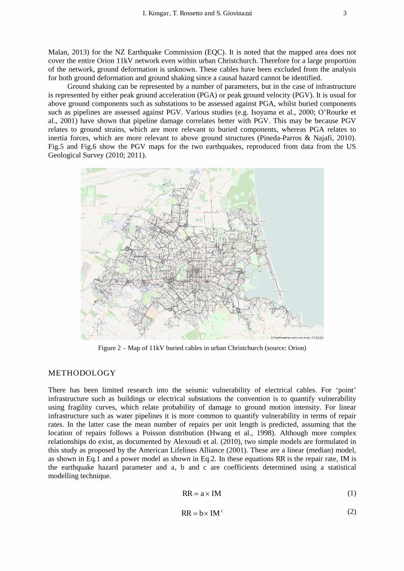
The 11kV network is classified into subtransmission and distribution cables. Thesubtransmission cables can be either feeder cables, which supply 11kV district/zone substations fromthe Transpower transmission network grid exit points, or primary cables, which supply networksubstations from district/zone substations. Distribution cables, also known as secondary cables, supplydistribution substations from network substations. However, in the following analysis, no distinction ismade between cables serving different operational functions. A map of the pre-earthquake network of11kV buried cables is shown in Fig.2.

EARTHQUAKE HAZARDS

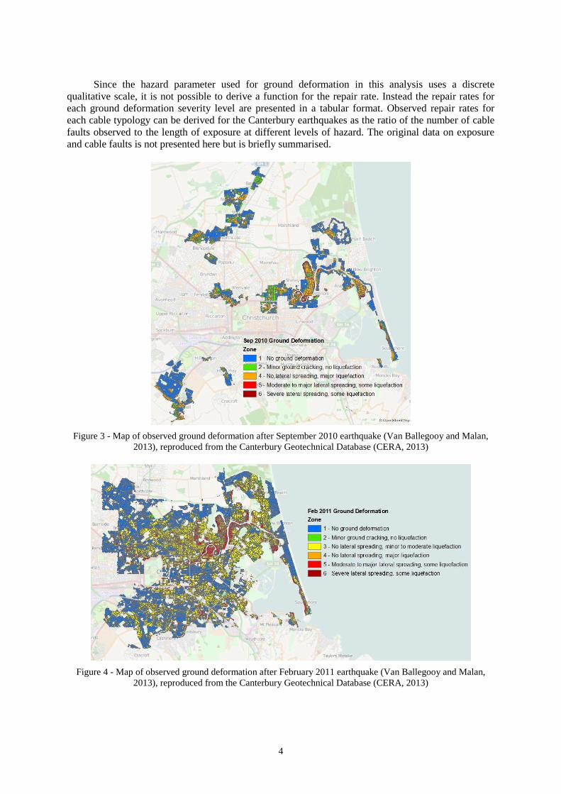
There are two earthquake hazards that may cause damage to electrical cables: ground shaking andground deformation (such as liquefaction or lateral spreading). Whilst in some areas of Christchurchground shaking was the only hazard, in other areas there was both ground shaking and grounddeformation. For this analysis it has been assumed that ground deformation is the controlling hazardfor buried infrastructure (O’Rourke et al., 2012), i.e. in areas where both ground shaking and grounddeformation occurred, deformation is assumed to be the main cause of damage to cables. Fig.3 andFig.4 show the ground deformation resulting from the two earthquakes as qualitative observations,published in the geotechnical study undertaken by consultants Tonkin & Taylor (Van Ballegooy and

I. Kongar, T. Rossetto and S. Giovinazzi 3

Malan, 2013) for the NZ Earthquake Commission (EQC). It is noted that the mapped area does notcover the entire Orion 11kV network even within urban Christchurch. Therefore for a large proportionof the network, ground deformation is unknown. These cables have been excluded from the analysisfor both ground deformation and ground shaking since a causal hazard cannot be identified.

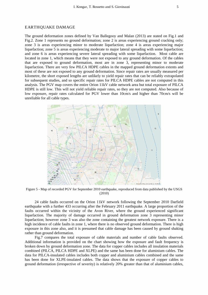
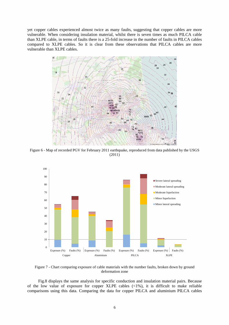
Ground shaking can be represented by a number of parameters, but in the case of infrastructureis represented by either peak ground acceleration (PGA) or peak ground velocity (PGV). It is usual forabove ground components such as substations to be assessed against PGA, whilst buried componentssuch as pipelines are assessed against PGV. Various studies (e.g. Isoyama et al., 2000; O’Rourke etal., 2001) have shown that pipeline damage correlates better with PGV. This may be because PGVrelates to ground strains, which are more relevant to buried components, whereas PGA relates toinertia forces, which are more relevant to above ground structures (Pineda-Parros & Najafi, 2010).Fig.5 and Fig.6 show the PGV maps for the two earthquakes, reproduced from data from the USGeological Survey (2010; 2011).

Figure 2 – Map of 11kV buried cables in urban Christchurch (source: Orion)

METHODOLOGY

There has been limited research into the seismic vulnerability of electrical cables. For ‘point’infrastructure such as buildings or electrical substations the convention is to quantify vulnerabilityusing fragility curves, which relate probability of damage to ground motion intensity. For linearinfrastructure such as water pipelines it is more common to quantify vulnerability in terms of repairrates. In the latter case the mean number of repairs per unit length is predicted, assuming that thelocation of repairs follows a Poisson distribution (Hwang et al., 1998). Although more complexrelationships do exist, as documented by Alexoudi et al. (2010), two simple models are formulated inthis study as proposed by the American Lifelines Alliance (2001). These are a linear (median) model,as shown in Eq.1 and a power model as shown in Eq.2. In these equations RR is the repair rate, IM isthe earthquake hazard parameter and a, b and c are coefficients determined using a statisticalmodelling technique.

RR a IM (1)

cRR b IM (2)

4

Since the hazard parameter used for ground deformation in this analysis uses a discretequalitative scale, it is not possible to derive a function for the repair rate. Instead the repair rates foreach ground deformation severity level are presented in a tabular format. Observed repair rates foreach cable typology can be derived for the Canterbury earthquakes as the ratio of the number of cablefaults observed to the length of exposure at different levels of hazard. The original data on exposureand cable faults is not presented here but is briefly summarised.

Figure 3 - Map of observed ground deformation after September 2010 earthquake (Van Ballegooy and Malan,2013), reproduced from the Canterbury Geotechnical Database (CERA, 2013)

Figure 4 - Map of observed ground deformation after February 2011 earthquake (Van Ballegooy and Malan,2013), reproduced from the Canterbury Geotechnical Database (CERA, 2013)

I. Kongar, T. Rossetto and S. Giovinazzi 5

EARTHQUAKE DAMAGE

The ground deformation zones defined by Van Ballegooy and Malan (2013) are stated on Fig.1 andFig.2. Zone 1 represents no ground deformation; zone 2 is areas experiencing ground cracking only;zone 3 is areas experiencing minor to moderate liquefaction; zone 4 is areas experiencing majorliquefaction; zone 5 is areas experiencing moderate to major lateral spreading with some liquefaction;and zone 6 is areas experiencing severe lateral spreading with some liquefaction. Most cable arelocated in zone 1, which means that they were not exposed to any ground deformation. Of the cablesthat are exposed to ground deformation, most are in zone 3, representing minor to moderateliquefaction. There are very few PILCA HDPE cables in the mapped ground deformation extents andmost of these are not exposed to any ground deformation. Since repair rates are usually measured perkilometre, the short exposed lengths are unlikely to yield repair rates that can be reliably extrapolatedfor subsequent studies, and so specific repair rates for PILCA HDPE cables are not computed in thisanalysis. The PGV map covers the entire Orion 11kV cable network area but total exposure of PILCAHDPE is still low. This will not yield reliable repair rates, so they are not computed. Also because oflow exposure, repair rates calculated for PGV lower than 10cm/s and higher than 70cm/s will beunreliable for all cable types.

Figure 5 - Map of recorded PGV for September 2010 earthquake, reproduced from data published by the USGS(2010)

24 cable faults occurred on the Orion 11kV network following the September 2010 Darfieldearthquake with a further 433 occurring after the February 2011 earthquake. A large proportion of thefaults occurred within the vicinity of the Avon River, where the ground experienced significantliquefaction. The majority of damage occurred in ground deformation zone 3 representing minorliquefaction; however zone 3 was also the zone containing the greatest network exposure. There is ahigh incidence of cable faults in zone 1, where there is no observed ground deformation. There is highexposure in this zone also, and it is presumed that cable damage has been caused by ground shakingrather than ground deformation.

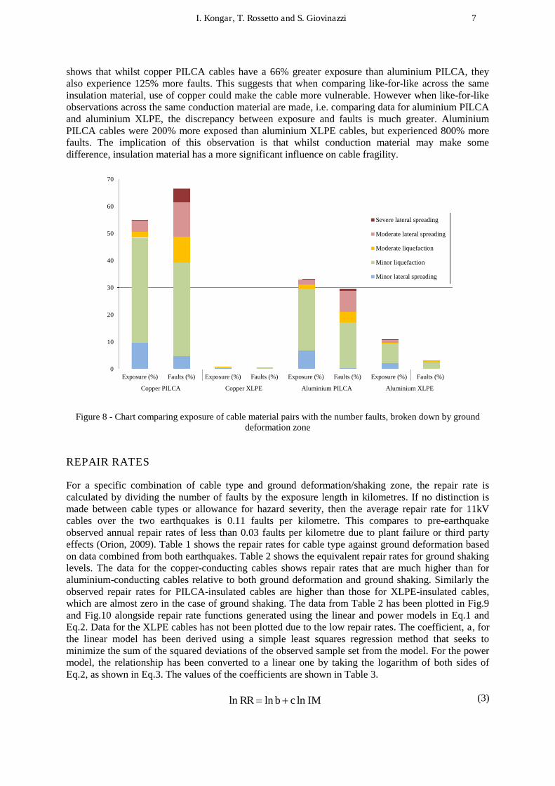
Fig.7 compares the total exposure of cable materials and number of cable faults observed.Additional information is provided on the chart showing how the exposure and fault frequency isbroken down by ground deformation zone. The data for copper cables includes all insulation materialscombined (PILCA, PILCA HDPE and XLPE) and the same has been done for aluminium cables. Thedata for PILCA-insulated cables includes both copper and aluminium cables combined and the samehas been done for XLPE-insulated cables. The data shows that the exposure of copper cables toground deformation (irrespective of severity) is relatively 20% greater than that of aluminium cables,

6

yet copper cables experienced almost twice as many faults, suggesting that copper cables are morevulnerable. When considering insulation material, whilst there is seven times as much PILCA cablethan XLPE cable, in terms of faults there is a 25-fold increase in the number of faults in PILCA cablescompared to XLPE cables. So it is clear from these observations that PILCA cables are morevulnerable than XLPE cables.

Figure 6 - Map of recorded PGV for February 2011 earthquake, reproduced from data published by the USGS(2011)

0

10

20

30

40

50

60

70

80

90

100

Exposure (%) Faults (%) Exposure (%) Faults (%) Exposure (%) Faults (%) Exposure (%) Faults (%)

Copper Aluminium PILCA XLPE

Severe lateral spreading

Moderate lateral spreading

Moderate liquefaction

Minor liquefaction

Minor lateral spreading

Figure 7 - Chart comparing exposure of cable materials with the number faults, broken down by grounddeformation zone

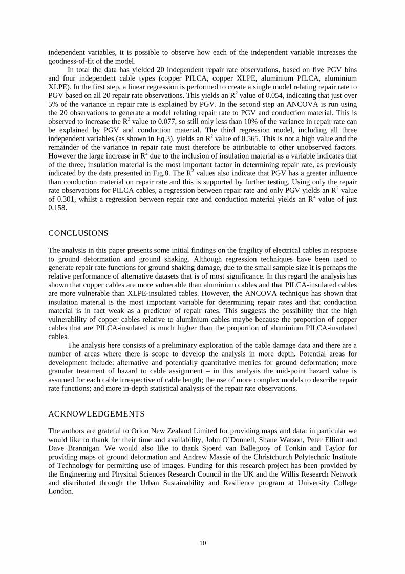
Fig.8 displays the same analysis for specific conduction and insulation material pairs. Becauseof the low value of exposure for copper XLPE cables (<1%), it is difficult to make reliablecomparisons using this data. Comparing the data for copper PILCA and aluminium PILCA cables

I. Kongar, T. Rossetto and S. Giovinazzi 7

shows that whilst copper PILCA cables have a 66% greater exposure than aluminium PILCA, theyalso experience 125% more faults. This suggests that when comparing like-for-like across the sameinsulation material, use of copper could make the cable more vulnerable. However when like-for-likeobservations across the same conduction material are made, i.e. comparing data for aluminium PILCAand aluminium XLPE, the discrepancy between exposure and faults is much greater. AluminiumPILCA cables were 200% more exposed than aluminium XLPE cables, but experienced 800% morefaults. The implication of this observation is that whilst conduction material may make somedifference, insulation material has a more significant influence on cable fragility.

0

10

20

30

40

50

60

70

Exposure (%) Faults (%) Exposure (%) Faults (%) Exposure (%) Faults (%) Exposure (%) Faults (%)

Copper PILCA Copper XLPE Aluminium PILCA Aluminium XLPE

Severe lateral spreading

Moderate lateral spreading

Moderate liquefaction

Minor liquefaction

Minor lateral spreading

Figure 8 - Chart comparing exposure of cable material pairs with the number faults, broken down by grounddeformation zone

REPAIR RATES

For a specific combination of cable type and ground deformation/shaking zone, the repair rate iscalculated by dividing the number of faults by the exposure length in kilometres. If no distinction ismade between cable types or allowance for hazard severity, then the average repair rate for 11kVcables over the two earthquakes is 0.11 faults per kilometre. This compares to pre-earthquakeobserved annual repair rates of less than 0.03 faults per kilometre due to plant failure or third partyeffects (Orion, 2009). Table 1 shows the repair rates for cable type against ground deformation basedon data combined from both earthquakes. Table 2 shows the equivalent repair rates for ground shakinglevels. The data for the copper-conducting cables shows repair rates that are much higher than foraluminium-conducting cables relative to both ground deformation and ground shaking. Similarly theobserved repair rates for PILCA-insulated cables are higher than those for XLPE-insulated cables,which are almost zero in the case of ground shaking. The data from Table 2 has been plotted in Fig.9and Fig.10 alongside repair rate functions generated using the linear and power models in Eq.1 andEq.2. Data for the XLPE cables has not been plotted due to the low repair rates. The coefficient, a, forthe linear model has been derived using a simple least squares regression method that seeks tominimize the sum of the squared deviations of the observed sample set from the model. For the powermodel, the relationship has been converted to a linear one by taking the logarithm of both sides ofEq.2, as shown in Eq.3. The values of the coefficients are shown in Table 3.

ln ln lnRR b c IM (3)

8

Table 1 - Repair rates for cable types by ground deformation zone. In the column for conduction material, ‘all’refers to data for copper and aluminium cables combined. In the column for insulation material, ‘all’ refers to

data for PILCA, PILCA HDPE and XLPE cables combined.

Conductionmaterial

Insulationmaterial

Repair rates (faults per km) by ground deformation zone1 2 3 4 5 6

Copper All 0.08 0.23 0.44 1.93 1.55 6.37Copper PILCA 0.08 0.23 0.43 2.05 1.56 6.62Copper XLPE 0.00 0.00 0.81 0.00 n/a n/aAluminium All 0.02 0.02 0.32 1.14 1.41 1.38Aluminium PILCA 0.04 0.03 0.36 1.08 2.10 7.08Aluminium XLPE 0.01 0.00 0.16 1.39 0.00 0.00All PILCA 0.06 0.15 0.41 1.63 1.73 6.67All XLPE 0.01 0.00 0.20 1.00 0.00 0.00

Table 2 - Repair rates for cable types by ground shaking zone. In the column for conduction material, ‘all’ refersto data for copper and aluminium cables combined. In the column for insulation material, ‘all’ refers to data for

PILCA, PILCA HDPE and XLPE cables combined.

Conductionmaterial

Insulationmaterial

Repair rates (faults per km) by ground shaking PGV (cm/s)11-20 21-30 31-40 41-50 51-60 61-70 71-80 81-90

Copper All 0.07 0.00 0.04 0.04 0.09 0.16 0.00 0.00Copper PILCA 0.07 0.00 0.04 0.04 0.09 0.16 0.00 0.00Copper XLPE 0.00 n/a 0.00 0.00 0.00 0.00 n/a n/aAluminium All 0.01 0.00 0.05 0.03 0.04 0.04 0.00 0.00Aluminium PILCA 0.00 0.00 0.08 0.04 0.07 0.05 0.00 0.00Aluminium XLPE 0.02 0.00 0.00 0.00 0.00 0.00 0.00 0.00All PILCA 0.04 0.00 0.05 0.04 0.08 0.13 0.00 0.00All XLPE 0.02 0.00 0.00 0.00 0.00 0.00 0.00 0.00

0.00

0.02

0.04

0.06

0.08

0.10

0.12

0.14

0.16

0.18

0 10 20 30 40 50 60 70

Re

pa

irra

te(f

au

lts

pe

rk

m)

PGV (cm/s)

Copper

Aluminium

PILCA

Copper PILCA

Aluminium PILCA

Copper (lin)

Aluminium (lin)

PILCA (lin)

Copper PILCA (lin)

Aluminium PILCA (lin)

Figure 9 – Observed repair rates from September 2010 and February 2011 earthquakes and derived repair ratefunctions using a linear model

Given the small observation sample size, the modelled repair rate functions should be treatedwith caution and in this respect it is the relative nature of the functions rather than the specificcalculated coefficients that are most informative. The functions developed using the power modelshow significant problems, with the slope for aluminium PILCA cables following a negative gradient.This indicates that the power model, in the form assumed here, is not appropriate for modelling cable

I. Kongar, T. Rossetto and S. Giovinazzi 9

repair rates from this data set. The functions derived using the linear model follow the expectedpattern with an increase in repair rate as the PGV increases for all cable types.

0.00

0.02

0.04

0.06

0.08

0.10

0.12

0.14

0.16

0.18

0 10 20 30 40 50 60 70

Re

pa

irra

te(f

au

lts

pe

rk

m)

PGV (cm/s)

Copper

Aluminium

PILCA

Copper PILCA

Aluminium PILCA

Copper (pow)

Aluminium (pow)

PILCA (pow)

Copper PILCA (pow)

Aluminium PILCA (pow)

Figure 10 – Observed repair rates from September 2010 and February 2011 earthquakes and derived repair ratefunctions using a power model

Table 3 – Coefficients of repair rate functions derived from linear and power models

Conductionmaterial

Insulationmaterial

Linear model Power modela b c

Copper All 0.001791 0.015245 0.406211Aluminium All 0.000692 0.000252 1.262547All PILCA 0.001596 0.004484 0.715857Copper PILCA 0.001816 0.015268 0.410730Aluminium PILCA 0.001088 0.492147 -0.555533

In the analysis so far, separate repair rate functions have been produced for each cable typerelating repair rate to PGV in a bivariate analysis. However an alternative approach is to generate asingle repair rate function that links repair rate to all three variable parameters: PGV, conductionmaterial and insulation material. In this multivariate analysis, categorical variables such as materialcan be represented by a dummy variable, taking a value of 0 or 1, depending on the material. Since theindependent variables are a mixture of quantitative (PGV) and qualitative (conduction and insulationmaterial), an Analysis of Covariance (ANCOVA) is conducted. The ANCOVA is run using theXLSTAT14 add-in for Microsoft Excel and produced the linear regression equation shown in Eq.4with a zero-intercept constraint. In this equation CMAT is a dummy variable for conduction material,taking a value of 0 for copper and 1 for aluminium, and IMAT is a dummy variable for insulationmaterial, taking a value of 0 for XLPE and 1 for PILCA.

0.000321 0.0177 0.0581RR PGV CMAT IMAT (4)

The multivariate approach also enables analysis of the relative importance of each of theindependent variables. Calculation of the coefficient of determination, known as R-squared (R2),indicates how well data points fit a statistical model such as a linear regression. The value of R2

represents the amount of variance in the dependent variable that is explained by variance in theindependent variables. If the R2 value is calculated initially for a regression model using only one ofthe independent variables and then repeated for regression models using two of and then all three

10

independent variables, it is possible to observe how each of the independent variable increases thegoodness-of-fit of the model.

In total the data has yielded 20 independent repair rate observations, based on five PGV binsand four independent cable types (copper PILCA, copper XLPE, aluminium PILCA, aluminiumXLPE). In the first step, a linear regression is performed to create a single model relating repair rate toPGV based on all 20 repair rate observations. This yields an R2 value of 0.054, indicating that just over5% of the variance in repair rate is explained by PGV. In the second step an ANCOVA is run usingthe 20 observations to generate a model relating repair rate to PGV and conduction material. This isobserved to increase the R2 value to 0.077, so still only less than 10% of the variance in repair rate canbe explained by PGV and conduction material. The third regression model, including all threeindependent variables (as shown in Eq.3), yields an R2 value of 0.565. This is not a high value and theremainder of the variance in repair rate must therefore be attributable to other unobserved factors.However the large increase in R2 due to the inclusion of insulation material as a variable indicates thatof the three, insulation material is the most important factor in determining repair rate, as previouslyindicated by the data presented in Fig.8. The R2 values also indicate that PGV has a greater influencethan conduction material on repair rate and this is supported by further testing. Using only the repairrate observations for PILCA cables, a regression between repair rate and only PGV yields an R2 valueof 0.301, whilst a regression between repair rate and conduction material yields an R2 value of just0.158.

CONCLUSIONS

The analysis in this paper presents some initial findings on the fragility of electrical cables in responseto ground deformation and ground shaking. Although regression techniques have been used togenerate repair rate functions for ground shaking damage, due to the small sample size it is perhaps therelative performance of alternative datasets that is of most significance. In this regard the analysis hasshown that copper cables are more vulnerable than aluminium cables and that PILCA-insulated cablesare more vulnerable than XLPE-insulated cables. However, the ANCOVA technique has shown thatinsulation material is the most important variable for determining repair rates and that conductionmaterial is in fact weak as a predictor of repair rates. This suggests the possibility that the highvulnerability of copper cables relative to aluminium cables maybe because the proportion of coppercables that are PILCA-insulated is much higher than the proportion of aluminium PILCA-insulatedcables.

The analysis here consists of a preliminary exploration of the cable damage data and there are anumber of areas where there is scope to develop the analysis in more depth. Potential areas fordevelopment include: alternative and potentially quantitative metrics for ground deformation; moregranular treatment of hazard to cable assignment – in this analysis the mid-point hazard value isassumed for each cable irrespective of cable length; the use of more complex models to describe repairrate functions; and more in-depth statistical analysis of the repair rate observations.

ACKNOWLEDGEMENTS

The authors are grateful to Orion New Zealand Limited for providing maps and data: in particular wewould like to thank for their time and availability, John O’Donnell, Shane Watson, Peter Elliott andDave Brannigan. We would also like to thank Sjoerd van Ballegooy of Tonkin and Taylor forproviding maps of ground deformation and Andrew Massie of the Christchurch Polytechnic Instituteof Technology for permitting use of images. Funding for this research project has been provided bythe Engineering and Physical Sciences Research Council in the UK and the Willis Research Networkand distributed through the Urban Sustainability and Resilience program at University CollegeLondon.

I. Kongar, T. Rossetto and S. Giovinazzi 11

REFERENCES

Alexoudi M, Pitilakis K and Souli A (2010) SYNER-G Deliverable D3.5: Fragility Functions for Water and

Wastewater System Elements, Aristotle University of Thessaloniki, Greece

American Lifelines Alliance (2001) Seismic Fragility Formulations for Water SystemsCanterbury Earthquake Recovery Authority (CERA) (2013) Canterbury Geotechnical Database,

https://canterburygeotechnicaldatabase.projectorbit.com/Registration/Login.aspx?ReturnUrl=%2fAccessed 12 November 2013

Eidinger J and Tang AK (2012) Christchurch, New Zealand Earthquake Sequence, MW 7.1 September 04, 2010,MW 6.3 February 22, 2011, MW 6.0 June 13, 2011, Lifelines Performance, Technical Council on LifelineEarthquake Engineering, ASCE, Reston, Virginia

Hwang HHM, Lin H and Shinozuka M (1998) “Seismic performance assessment of water delivery systems”,Journal of Infrastructure Systems, 4:118-125

Isoyama R, Ishida E, Yune K and Shirozu T (2000) “Seismic damage estimation procedure for water supply

pipelines”, Proceedings of the 12th World Conference on Earthquake Engineering, Auckland, New

Zealand, 30 January – 4 February

O’Rourke TD, Stewart HE and Jeon S-S (2001) “Geotechnical aspects of lifelines engineering”, GeotechnicalEngineering, 149(1):13-26

O’Rourke TD, Jeon S-S, Toprak S, Cubrinovski M and Jung JK (2012) “Underground lifeline systemperformance during the Canterbury earthquake sequence”, Proceedings of the 15th World Conference onEarthquake Engineering, Lisbon, Portugal, 24-28 September

Orion (2009) Asset Management Plan, Orion New Zealand Limited, Christchurch, New Zealand.Massie, A (2014) High Voltage Learning During the Christchurch Earthquakes,

http://www.thunderboltnz.blogspot.com Accessed 24 March 2014

Pineda-Porras O and Najafi M (2010) “Seismic damage estimation for buried pipelines: challenges after three

decades of progress”, Journal of Pipeline Systems Engineering, 1:19–24

US Geological Survey (USGS) (2010) USGS ShakeMap: South Island of New Zealand Saturday September 4th,2010 http://earthquake.usgs.gov/earthquakes/shakemap/global/shake/2010atbj/ Accessed 1 May 2013

US Geological Survey (USGS) (2011) USGS ShakeMap: South Island of New Zealand Tuesday February 22nd,2011 http://earthquake.usgs.gov/earthquakes/shakemap/global/shake/b0001igm/ Accessed 1 May 2013

Van Ballegooy S and Malan P (2013) Earthquake Commission: Liquefaction Vulnerability Study, Tonkin andTaylor Ltd., Christchurch, New Zealand