seismic response modeling of water supply systems

ISSN 1520-295X

Seismic Response Modeling of Water Supply Systems

by Peixin Shi and Thomas D. O’Rourke

Technical Report MCEER-08-0016

May 5, 2008

This research was conducted at Cornell Universityand was supported primarily by the Earthquake Engineering Research Centers

Program of the National Science Foundation under award number EEC 9701471.

NOTICEThis report was prepared by Cornell University as a result of research spon-sored by MCEER through a grant from the Earthquake Engineering Research Centers Program of the National Science Foundation under NSF award number EEC-9701471 and other sponsors. Neither MCEER, associates of MCEER, its sponsors, Cornell University, nor any person acting on their behalf:

a. makes any warranty, express or implied, with respect to the use of any information, apparatus, method, or process disclosed in this report or that such use may not infringe upon privately owned rights; or

b. assumes any liabilities of whatsoever kind with respect to the use of, or the damage resulting from the use of, any information, apparatus, method, or process disclosed in this report.

Any opinions, findings, and conclusions or recommendations expressed in this publication are those of the author(s) and do not necessarily reflect the views of MCEER, the National Science Foundation, or other sponsors.

Seismic Response Modeling of Water Supply Systems

by

Peixin Shi1 and Thomas D. O’Rourke2

Publication Date: May 5, 2008 Submittal Date: March 28, 2008

Technical Report MCEER-08-0016

Task Number 10.1.2

NSF Master Contract Number EEC 9701471

1 Geotechnical Engineer, PB Americas, Inc., Geotechnical and Tunneling Group; for-mer Ph.D. Candidate, School of Civil and Environmental Engineering, Cornell Uni-versity

2 Thomas R. Briggs Professor of Engineering, School of Civil and Environmental Engi-neering, Cornell University

MCEERUniversity at Buffalo, The State University of New YorkRed Jacket Quadrangle, Buffalo, NY 14261Phone: (716) 645-3391; Fax (716) 645-3399E-mail: [email protected]; WWW Site: http://mceer.buffalo.edu

iii

Preface

The Multidisciplinary Center for Earthquake Engineering Research (MCEER) is a national center of excellence in advanced technology applications that is dedicated to the reduction of earthquake losses nationwide. Headquartered at the University at Buffalo, State University of New York, the Center was originally established by the National Science Foundation in 1986, as the National Center for Earthquake Engineering Research (NCEER).

Comprising a consortium of researchers from numerous disciplines and institutions throughout the United States, the Center’s mission is to reduce earthquake losses through research and the application of advanced technologies that improve engineering, pre-earthquake planning and post-earthquake recovery strategies. Toward this end, the Cen-ter coordinates a nationwide program of multidisciplinary team research, education and outreach activities.

MCEER’s research is conducted under the sponsorship of two major federal agencies: the National Science Foundation (NSF) and the Federal Highway Administration (FHWA), and the State of New York. Signifi cant support is derived from the Federal Emergency Management Agency (FEMA), other state governments, academic institutions, foreign governments and private industry.

MCEER’s NSF-sponsored research objectives are twofold: to increase resilience by devel-oping seismic evaluation and rehabilitation strategies for the post-disaster facilities and systems (hospitals, electrical and water lifelines, and bridges and highways) that society expects to be operational following an earthquake; and to further enhance resilience by developing improved emergency management capabilities to ensure an effective response and recovery following the earthquake (see the fi gure below).

-

Infrastructures that Must be Available /Operational following an Earthquake

Intelligent Responseand Recovery

Hospitals

Water, GasPipelines

Electric PowerNetwork

Bridges andHighways

MoreEarthquake

Resilient UrbanInfrastructure

System

Cost-EffectiveRetrofit

Strategies

Earthquake Resilient CommunitiesThrough Applications of Advanced Technologies

iv

A cross-program activity focuses on the establishment of an effective experimental and analytical network to facilitate the exchange of information between researchers located in various institutions across the country. These are complemented by, and integrated with, other MCEER activities in education, outreach, technology transfer, and industry partnerships.

This report presents a comprehensive model for simulating the earthquake performance of water supply systems. The model is developed in conjunction with the water system operated by the Los Angeles Department of Water and Power (LADWP) and validated through comparisons to ob-servations and fl ow measurements for the heavily damaged LADWP water supply after the 1994 Northridge earthquake. The earthquake performance of damaged water supply systems is simulated using hydraulic network analysis that uses an iterative approach to isolate the network nodes with negative pressures. The isolation process accounts accurately for reliable fl ows and pressures in the damaged water networks by removing unreliable fl ows and identifying those portions of the system requiring mitigation. An analytical model is developed to predict the effect of seismic waves on underground pipelines. The seismic performance of the LADWP system is simulated using a multi-scale technique in which the LADWP trunk system is explicitly accounted for, while the remaining distribution lines are simulated through fragility curves relating demand to repair rate. The repair rate, in turn, is correlated with peak ground velocities, and fragility curves are developed on the basis of distribution network simulations. The proposed model is integrated into computer code, Graphical Iterative Response Analysis for Flow Following Earthquakes (GIRAFFE) developed by the authors, which presents the simulation results in GIS format.

v

ABSTRACT

This report describes a comprehensive model for simulating the earthquake

performance of water supply systems. This model is developed in conjunction with the

water supply system operated by the Los Angeles Department of Water and Power

(LADWP) and validated by a favorable comparison of simulation results with

observations and flow measurements for the heavily damaged LADWP water supply

after the 1994 Northridge earthquake.

Earthquake performance of water supply systems is simulated using hydraulic

network analysis. Hydraulic simulation procedures for heavily damaged water supply

systems are developed on the basis of an iterative approach to isolate the network

nodes with negative pressures step by step, starting with the one of highest negative

pressure. The isolation approach accounts accurately for reliable flows and pressures

in the damaged system. The isolation approach removes unreliable flows, and

identifies vulnerable parts of the damaged system for mitigation.

To predict earthquake damage to underground water supply pipelines, an

analytical model is developed for surface wave interaction with jointed concrete

cylinder pipelines (JCCPs). A dimensionless chart is developed for estimating the joint

pullout of JCCPs under the action of seismic waves. This model is applied to analyze

seismic wave interaction with other jointed pipelines, such as cast iron (CI) pipelines

with lead-caulked joints. Dimensionless reduction curves are developed for estimating

joint pullout associated with brittle and ductile joint performance.

Pipeline damage in hydraulic simulations is classified as breaks and leaks. A

break is simulated by disconnecting the original pipeline completely and opening the

broken ends into the atmosphere; a leak is simulated as an orifice in the pipe wall.

Energy loss from the leak is accounted for as minor losses. Five different scenarios of

leakage are simulated as a function of pipe diameter.

vi

Seismic performance of the LADWP system is simulated using a multi-scale

technique. This technique explicitly accounts for 2,200 km of pipelines, associated

with the LADWP trunk system, and simulates the remaining 9,800 km of distribution

lines by fragility curves relating demand to repair rate in the distribution network.

Repair rate, in turn, is correlated with peak ground velocity. The fragility curves are

developed on the basis of LADWP distribution network simulations.

A computer code, GIRAFFE, is developed for the implementation of the

model. GIRAFFE builds on an open source hydraulic network analysis engine,

EPANET, and works in conjunction with Geographical Information Systems (GIS) for

simulation result presentations.

vii

ACKNOWLEDGMENTS

This research was funded by the Earthquake Engineering Research Centers

Program of the National Science Foundation (NSF) through the Multidisciplinary

Center for Earthquake Engineering Research (MCEER). The financial support from

the NSF and MCEER is gratefully acknowledged.

Thanks and acknowledgements are given to the Los Angeles Department of

Water and Power (LADWP) engineers, namely Mr. Collins Anselmo, Mr. Craig Davis,

Mr. Paul Gillis, Mr. Vargas Victor, and others whose names I might have inadvertently

missed, for providing information on the LADWP water supply system, the 1994

Northridge earthquake trunk line damage, and the SCADA data.

TABLE OF CONTENTS

Chapter Title Page

ix

1 INTRODUCTION ......................................................................... 1

1.1 Background ...................................................................................... 1

1.2 Objectives ........................................................................................ 7

1.2.1 Hydraulic Network Analysis for Damaged Systems ....................... 7

1.2.2 Seismic Response of Buried Pipelines to Surface Wave Effects .... 8

1.2.3 Pipe Damage Modeling ................................................................... 9

1.2.4 Multi-Scale Technique for Water Supply System Modeling .......... 9

1.2.5 Evaluation of Northridge Earthquake Performance ...................... 10

1.3 Scope ............................................................................................. 10

2 HYDRAULIC NETWORK ANALYSIS FOR UNDAMAGED

SYSTEMS ................................................................................... 13

2.1 Introduction ................................................................................... 13

2.2 Components in Hydraulic Networks ............................................. 14

2.3 Fundamentals of Fluid Mechanics ................................................. 15

2.3.1 Fluid Properties ............................................................................. 16

2.3.2 Flow Regime ................................................................................. 18

2.3.3 Fluid Energy .................................................................................. 21

2.3.4 Energy Losses ................................................................................ 22

2.3.4.1 Frictional Loss ............................................................................... 22

2.3.4.2 Minor Loss ..................................................................................... 25

2.3.5 Energy Gains ................................................................................. 26

2.3.6 Principle Laws of Flow Analysis .................................................. 27

2.3.6.1 Equation of Continuity .................................................................. 28

2.3.6.2 Bernoulli Equation ......................................................................... 29

2.4 Flow Equations .............................................................................. 30

2.4.1 Q-equations .................................................................................... 30

2.4.2 H-equations .................................................................................... 31

2.4.3 ΔQ-equations ................................................................................. 32

2.4.4 Hybrid equations ........................................................................... 33

TABLE OF CONTENTS (Cont’d)

Chapter Title Page

x

2.5 Numerical Methods for Flow Equations ....................................... 34

2.5.1 Hardy-Cross Method ..................................................................... 34

2.5.2 Newton-Raphson Method .............................................................. 36

2.5.3 Linear Theory Method ................................................................... 38

2.5.4 Gradient Method ............................................................................ 40

2.6 Hydraulic Network Analysis Software .......................................... 42

2.6.1 EPANET ........................................................................................ 42

2.6.1.1 EPANET Hydraulic Network Components ................................... 43

2.6.1.2 EPANET Input File ....................................................................... 48

2.6.1.3 EPANET Hydraulic Simulation Methodology .............................. 50

2.6.1.4 EPANET Output File .................................................................... 50

2.6.1.5 An Example of EPANET Simulation ............................................ 51

2.6.2 H2ONET ........................................................................................ 52

2.6.3 Limitations of Commercial Software Packages ............................ 59

2.6.3.1 Negative Pressure Prediction ......................................................... 59

2.6.3.2 Pipe Damage Simulation ............................................................... 60

3 HYDRAULIC NETWORK ANALYSIS FOR DAMAGED

SYSTEMS .................................................................................... 61

3.1 Introduction ................................................................................... 61

3.2 Negative Pressure Generation ....................................................... 62

3.3 Previous Research ......................................................................... 69

3.3.1 Ballantyne et al. Approach ............................................................ 69

3.3.2 Shinozuka et al. Approach ............................................................. 70

3.3.3 Markov et al. Approach ................................................................. 70

3.3.4 Discussions of the Three Approaches ........................................... 72

3.4 Current Approach .......................................................................... 74

4 SEISMIC RESPONSE OF BURIED PIPELINES TO


Chapter Title Page

xi

SURFACE WAVE EFFECTS .................................................... 77

4.1 Introduction ................................................................................... 77

4.2 Seismic Hazards to Buried Pipelines ............................................. 78

4.2.1 Seismic Wave Hazards .................................................................. 78

4.2.2 Surface Wave Characteristics ........................................................ 81

4.3 Analytical Model for Surface Wave Interaction with JCCPs ........ 85

4.3.1 JCCPs ............................................................................................ 85

4.3.2 Performance of JCCPs during Previous Earthquakes ................... 87

4.3.3 Seismic Wave Interaction with JCCPs .......................................... 88

4.3.4 Finite Element Model .................................................................... 94

4.3.5 Universal Relationship ................................................................ 104

4.3.6 Concrete Cracking Effects ........................................................... 108

4.4 Analytical Model for Surface Wave Interaction with CI

Pipelines ...................................................................................... 116

4.4.1 CI Pipelines ................................................................................. 116

4.4.2 Seismic Wave Interaction with CI Pipelines ............................... 117

4.4.3 Finite Element Model .................................................................. 120

4.4.4 Relative Joint Displacement Reduction Curves .......................... 124

4.4.4.1 Normalized Parameters ............................................................... 124

4.4.4.2 Reduction Curves from FE Analyses .......................................... 125

4.4.4.3 Lower Bound ............................................................................... 127

4.4.4.4 Upper Bound ............................................................................... 129

4.4.4.5 Reduction Curves for Engineering Usage ................................... 131

5 PIPE DAMAGE MODELING ................................................. 135

5.1 Introduction ................................................................................. 135

5.2 Previous Research ....................................................................... 136

5.2.1 Ballantyne et al. Model ................................................................ 136

5.2.2 Hwang et al. Model ..................................................................... 137

5.2.3 Markov et al. Model .................................................................... 138


Chapter Title Page

xii

5.2.4 Discussions of the Three Models ................................................ 138

5.3 Definitions ................................................................................... 140

5.4 Pipe Leak Simulation .................................................................. 140

5.4.1 Methodology ................................................................................ 141

5.4.1.1 Theoretical Derivation ................................................................. 141

5.4.1.2 Validation Using Sprinkler Data ................................................. 143

5.4.2 Hydraulic Model .......................................................................... 146

5.4.3 Pipe Property and Damage Mechanism Review ......................... 147

5.4.3.1 Cast Iron Pipes ............................................................................. 147

5.4.3.2 Ductile Iron Pipes ........................................................................ 151

5.4.3.3 Riveted Steel Pipes ...................................................................... 151

5.4.3.4 Jointed Concrete Cylinder Pipes ................................................. 153

5.4.3.5 Welded Steel Pipes ...................................................................... 157

5.4.4 Leak Classification ...................................................................... 159

5.4.4.1 Annular Disengagement .............................................................. 159

5.4.4.2 Round Crack ................................................................................ 163

5.4.4.3 Longitudinal Crack ...................................................................... 164

5.4.4.4 Local Loss of Pipe Wall .............................................................. 166

5.4.4.5 Local Tear of Pipe Wall .............................................................. 167

5.4.5 Probability of Leak Scenarios ..................................................... 169

5.5 Pipe Break Simulation ................................................................. 171

5.6 Implementation of Pipe Damage Models .................................... 171

5.6.1 Deterministic Implementation ..................................................... 172

5.6.2 Probabilistic Implementation ....................................................... 172

5.6.2.1 Generating Pipe Damage ............................................................. 173

5.6.2.2 Deciding on Damage State .......................................................... 174

5.6.2.3 Determining Leak Type ............................................................... 174

6 MULTI-SCALE TECHNIQUE FOR WATER SUPPLY

SYSTEM MODELING ............................................................. 177


Chapter Title Page

xiii

6.1 Introduction ................................................................................. 177

6.2 Multi-Scale Modeling Technique ................................................ 178

6.3 LADWP System and Model Descriptions ................................... 182

6.3.1 LADWP Water Supply System ................................................... 182

6.3.2 LADWP Trunk System Model .................................................... 184

6.3.3 LADWP Distribution System Models ......................................... 185

6.4 Distribution Network Simulations ............................................... 188

6.4.1 Simulation Procedures ................................................................. 188

6.4.2 Simulation Results ....................................................................... 191

6.4.3 Fragility Curve Construction ....................................................... 195

6.4.3.1 Observations ................................................................................ 197

6.4.3.2 Mean Regression with Noise Term ............................................. 199

6.4.3.3 90% Confidence Level Regression ............................................. 204

6.4.4 Test of Fragility Curves ............................................................... 205

7 EVALUATION OF NORTHRIDGE EARTHQUAKE

PERFORMANCE ...................................................................... 209

7.1 Introduction ................................................................................. 209

7.2 GIRAFFE .................................................................................... 210

7.2.1 System Definition ........................................................................ 212

7.2.2 System Modification ................................................................... 212

7.2.3 System Damage ........................................................................... 213

7.2.3.1 Deterministic Simulation ............................................................. 213

7.2.3.2 Probabilistic Simulation .............................................................. 214

7.2.4 Earthquake Demand Simulation .................................................. 216

7.2.5 Hydraulic Network Analysis ....................................................... 217

7.2.6 Compilation of Results ................................................................ 218

7.2.6.1 Hydraulic Network Analysis Results .......................................... 218

7.2.6.2 Performance Index ....................................................................... 219

7.3 GIRAFFE Simulation of Northridge Earthquake Performance .. 219


Chapter Title Page

xiv

7.3.1 LADWP System Performance during Northridge Earthquake ... 220

7.3.2 LADWP Hydraulic Model for Northridge Earthquake ............... 222

7.3.3 Damage Simulation ..................................................................... 224

7.3.3.1 Trunk Line Damage ..................................................................... 224

7.3.3.2 Distribution Line Damage ........................................................... 225

7.3.3.3 Tank Damage ............................................................................... 228

7.3.3.4 Water-Electric Power Interaction ................................................ 230

7.3.4 SCADA Data ............................................................................... 230

7.3.4.1 Boundary Conditions ................................................................... 232

7.3.4.2 System Reconfiguration .............................................................. 232

7.3.4.3 Flow Comparison ........................................................................ 234

7.3.5 Simulation Results ....................................................................... 234

8 SUMMARY AND CONCLUSIONS ........................................ 241

8.1 Introduction ................................................................................. 241

8.2 Hydraulic Network Analysis for Damaged Systems ................... 242

8.3 Seismic Response of Buried Pipelines to Surface Wave Effects 243

8.4 Pipe Damage Modeling ............................................................... 245

8.5 Multi-Scale Technique for Water Supply System Modeling ...... 246

8.6 Evaluation of Northridge Earthquake Performance .................... 247

8.7 Future Research Directions ......................................................... 248

9 REFERENCES ................................................................. 251

Appendix A LADWP DISTRIBUTION NETWORK DESCRIPTIONS .. 263

Appendix B LADWP DISTRIBUTION NETWORK SIMULATION

RESULTS ................................................................................... 277

Appendix C LADWP TRUNK LINE DAMAGE SIMULATIONS ........... 285

LIST OF FIGURES

Figure Title Page

xv

2.1 Experimental Apparatus Used to Determine Reynolds Number 20

2.2 General Shape of Pump Characteristic Curve 27

2.3 Pump Operation Point 28

2.4 Physical Components in an EPANET Hydraulic Network 44

2.5 Hydraulic Network with Component IDs and Demands 52

2.6 Hydraulic Network Analysis Results from EPANET 56

2.7 Hydraulic Network Analysis Results from H2ONET

57

3.1 Hydraulic Network Analysis with Negative Pressures 63

3.2 Water Profile Around Partial-Flow Node 69

3.3 Negative Pressure Node Demonstration

72

4.1 R-Wave Propagation and Particle Motion Directions 80

4.2 Resolution of Particle and Phase Velocities Along the Pipeline Axial

Direction for R-Waves

81

4.3 North-South Velocity Histories in Hill and Lake Zones in Mexico City

during the 1985 Michoacan Earthquake

83

4.4 Soil Profile at Strong Motion Station, Central de Abastos-Oficinas, in

Mexico City

84

4.5 R-Wave Dispersion Curves for the Soil Profile Shown in Figure 4.4 84

4.6 Sinusoidal Wave Interaction with Pipe Element 89

4.7 Sinusoidal Wave Interaction with a Continuous Relatively Rigid Pipeline 91

4.8 Sinusoidal Wave Interaction with a Relatively Rigid Pipeline with a Cracked

Joint

93

4.9 Sinusoidal Wave Interaction with a Relatively Flexible Pipeline with a

Cracked Joint

95

4.10 Finite Element Model for Seismic Wave Interaction with Pipeline 96

4.11 Elasto-Plastic Model for Unit Shear Transfer Between Ground Soil and

Pipeline

97

LIST OF FIGURES (Cont’d)

Figure Title Page

xvi

4.12 FE Simulation of Ground and Pipeline Displacements for Surface Wave

Interaction with JCCP

101

4.13 FE Simulation of Pipeline-Ground Relative Displacement for Surface Wave


102

4.14 FE Simulation of Ground and Pipeline Strains for Surface Wave Interaction

with JCCP

103

4.15 Universal Relationship Between δ/δ0 and f/EAR 105

4.16 Process of Seismic Wave Interaction with Pipeline 109

4.17 Simplified View of Sinusoidal Wave Interaction with JCCP Considering

Concrete Cracking Effects

113

4.18 Axial Force vs. Displacement for Lead Caulked Joints 117

4.19 Sinusoidal Wave Interaction with CI Pipeline 118

4.20 Elasto-Plastic Model for Axial Force vs. Displacement for Lead Caulked

Joints

121

4.21 Pipe-Ground Relative Displacement for Sinusoidal Wave Interaction with CI

Pipeline

122

4.22 Pipe and Ground Strain for Sinusoidal Wave Interaction with CI Pipeline 123

4.23 Strain Response Curve for a Relatively Rigid Pipeline with Different Values

of (FJ /EA)/εPmax

125

4.24 Reduction Curves from FE Analysis Results 126

4.25 Strain Response Curves of a Relatively Flexible Pipeline 128

4.26 Strain Response Curves of a Relatively Rigid Pipeline 130

4.27 Reduction Curves for Engineering Usage

132

5.1 Longitudinal Section of a Leaking Pipe 142

5.2 Comparison Between Model Predictions and Sprinkler Data 145

5.3 Relationship Between CD and A1 for Leakage 146

5.4 Hydraulic Model for Pipe Leak 147

5.5 Cast Iron Pipe with Bell-and-Spigot Lead Caulked Joint 149

5.6 Schematic Drawing of Bell-and-Spigot Lead Caulked Joint Cross-Section 149


Figure Title Page

xvii

5.7 Ductile Iron Pipes with Bell-and-Spigot Push-On Joints 152

5.8 Schematic Drawing of Bell-and-Spigot Push-on Joint Cross-Section 152

5.9 Riveted Steel Pipeline 154

5.10 Schematic Drawings of Rivet Connections 154

5.11 Photo of JCCP and Joints 156

5.12 Schematic Drawing of JCCP Joint Cross-Section 156

5.13 Steel Pipe with Welded Slip Joint 158

5.14 Schematic Drawing of Welded Slip Joint Cross-Sections 158

5.15 Photo Showing Pipe Leak in a 3050-mm-Diameter Welded Steel Pipe 160

5.16 Photo Showing Removed Section of Pipe Wall with a 1.5-m-Split at Welded

Slip Joint

160

5.17 Schematic Drawing of Annular Disengagement at Bell-and-Spigot Joint 161

5.18 Schematic Drawing of Round Crack 163

5.19 Schematic Drawing of Longitudinal Crack 165

5.20 Schematic Drawing of Local Loss of Pipe Wall 167

5.21 Schematic Drawing of Local Tear of Pipe Wall 168

5.22 Water Loss for Five Leak Scenarios as a Function of Pipe Diameter 169

5.23 Hydraulic Model for Pipe Break 172

5.24 Poisson Process for Pipe Damage Generation

175

6.1 Example of a Simple Water Supply System 180

6.2 Multi-Scale Models for a Simple Water Supply System 180

6.3 LADWP Water Supply System 183

6.4 LADWP Trunk Line Model 183

6.5 Locations of the Six LADWP Distribution Systems 187

6.6 ND vs. RR Relationship for Various Damage States for Pipe 9 192

6.7 ND vs. RR Relationship for Various Damage States for Pipe 5 193

6.8 Relationship Between Normalized Demand and Repair Rate 195

6.9 Regression Relationship Between Mean Pressure and Slope 198

6.10 Regression Relationship Between Mean Pressure and Intercept 198

6.11 Regression Relationship Between Mean Pressure and Mean Slope 200


Figure Title Page

xviii

6.12 Regression Relationship Between Mean Pressure and Mean Intercept 200

6.13 Regression Relationship Between Mean Pressure and Standard Deviation of

the Slopes

201

6.14 Regression Relationship Between Mean Pressure and Standard Deviation of

Intercepts

201

6.15 Comparison Between Simulated and Predicted Results for Distribution

System 205

206

7.1 GIRAFFE Simulation Flow Chart 211

7.2 LADWP Damaged Tanks, Trunk and Distribution Line Repairs, and Water

Outage Areas after the Northridge Earthquake

221

7.3 LADWP Hydraulic Model for Northridge Earthquake Simulation 223

7.4 Normalized Demands of Valley-Six Subsystem after Northridge Earthquake 227

7.5 LADWP Tanks and Reservoirs, and Damaged Tanks after Northridge

Earthquake

229

7.6 Superposition of Spatial Distribution of Electricity Outage Time and Pump

Stations

231

7.7 System Damage and SCADA Flow Meters 233

7.8 GIRAFFE Simulation Results 235

7.9 Comparisons Between GIRAFFE Results and Monitored Data

236

A.1 Map Showing the Distribution System 1449 Hydraulic Network Model 265

A.2 Pie Chart Showing Distribution of Pipelines of Various Diameters in System

1449

266



1000

268



579

270

A.7 Map Showing the Distribution System 448 & 462 Hydraulic Network Model 271


Figure Title Page

xix


448 & 462

272



426

274



205

276

B.1 Simulation Results for Monitored Pipes in Distribution System 1449 279



B.4 Simulation Results for Monitored Pipes in Distribution System 448 & 462 282


B.6 Simulation Results for Monitored Pipes in Distribution System 205

284

C.1 Granada Trunk Line and Its Repairs 286

C.2 Rinaldi Trunk Line and Its Repairs 291

C.3 Roscoe Trunk Line and Its Repairs 294

C.4 Other Trunk Line Repairs in Van Norman Complex 297

C.5 Other Trunk Line Repairs outside Van Norman Complex 299

LIST OF TABLES

Table Title Page

xxi

2.1 Reynolds Number for Various Flow Regimes 21

2.2 Frictional Head Loss Evaluation Formulas 24

2.3 Summary Table for Physical Components in an EPANET Hydraulic

Network Model

45

2.4 Sections in an EPANET Input File 49

2.5 EPANET Input File 53

2.6 EPANET Output File 55

2.7 Comparison of Link Flow Rates Between EPANET and H2ONET Results 58

2.8 Comparison of Nodal Pressures Between EPANET and H2ONET Results

58

4.1 JCCP Physical Properties and Ground Conditions for FE Analysis 100

4.2 Summary Table for FE Analysis Parameters 106

4.3 CI Pipeline Physical Properties and Ground Conditions for FE Analysis

121

5.1 Relationship Between Sprinkler Discharge Coefficient and Orifice Size 145

5.2 Probability of Leak Scenarios for Different Types of Pipelines

171

6.1 Simulation Results for Five Representative Distribution Networks in

LADWP System

196

C.1 Granada Trunk Line Damage Information Summary 287

C.2 Rinaldi Trunk Line Damage Information Summary 292

C.3 Roscoe Trunk Line Damage Information Summary 295

C.4 Other Trunk Line Damage Information Summary 1 298

C.5 Other Trunk Line Damage Information Summary 2 300

1

CHAPTER 1

INTRODUCTION

1.1 BACKGROUND

Water supplies constitute a key component of critical civil infrastructure that

supports fire protection and provide water for potable household consumption as well

as industrial and commercial uses. Water is conveyed mostly in underground

pipelines. Thus, ground movements triggered by earthquakes have a direct effect on

the integrity and reliability of water distribution networks. Water supplies are

vulnerable to earthquakes. This vulnerability has been demonstrated by extensive

damage sustained during previous earthquakes, such as the 1906 San Francisco (e.g.,

Schussler, 1906; Manson, 1908; Lawson, 1908; Scawthorn, et al., 2006), 1971 San

Fernando (e.g., Steinbrugge, et al., 1971; Subcommittee on Water and Sewerage

Systems, 1973; Eguchi, 1982), and 1994 Northridge (e.g., Lund and Cooper, 1995;

Hall, 1995; Eguchi and Chung, 1995; O’Rourke, et al., 2001) earthquakes.

Earthquake damage to water supply systems may disrupt residential, commercial, and

industrial activities; impair fire-fighting capacities; and prolong local community

recovery in the aftermath of earthquakes. It is very important, therefore, to model the

earthquake performance of water supply systems in a robust and reliable way for

emergency planning, community restoration, and assessment of regional economic

impacts.

There has been extensive work performed on the seismic modeling of water

supply systems. Early studies focused on component behavior and simple system

2

models (e.g., Hall and Newmark, 1977; Wright and Takada, 1980; Hwang and Lysmer,

1981; O’Rourke, 1998). As more advanced experimental and computational modeling

was developed, network simulations were explored to assess system reliability and

serviceability (e.g., Eguchi, et al., 1983; Ballantyne, et al., 1990; Khater and Grigoriu,

1989; Markov, et al., 1994; Shinozuka, et al., 1981, 1992, 1998; Hwang, et al., 1998;

Chang, et al., 2000).

Water supplies are large, geographically dispersed systems that are composed

of many different types of pipelines as well as other supporting facilities, such as tanks,

reservoirs, pumping stations, and regulator stations. Moreover, water supplies are

subject to seismic and geotechnical loading conditions associated with spatially

variable ground conditions, seismic sources, and source to site pathways for seismic

waves. It is not possible to model such systems in a deterministic manner, and thus

probabilistic methods have been developed to characterize system performance.

Scenario earthquakes for evaluating system performance are often chosen on the basis

of recurrence interval so that the seismic hazard can be linked with the probability of

exceedance within a certain time span, often taken as 50 years (Frankel, et al., 1996).

The response of a lifeline system to various seismic hazards is often assessed in a

probabilistic way because it is not possible a priori to predict where damage will

occur, although it is possible to estimate average rates of repair under various extreme

event conditions. Monte Carlo simulations are performed to predict system response,

followed by the probabilistic characterization of system reliability and serviceability.

The probabilistic approach has been applied to evaluate the seismic performance of

the water supply system operated by Memphis Light, Water and Gas (MLWG) in

Memphis and Shelby County, TN, by Shinozuka, et al. (1998) and Chang, et al. (2000),

3

as well as the Auxiliary Water Supply System (AWSS) in San Francisco by Khater

and Grigoriu (1989) and Markov, et al. (1994).

A key feature of modern water supply system modeling is the use of

geographic information systems (GIS). The rapid development of computer mapping

and visualization tools, embodied in GIS, provides a powerful basis for evaluating

earthquake effects on water supplies. GIS has become an engine for driving new

methodologies and decision support tools focused on the spatial variation of

earthquake effects. The Japan Water Works Association (1996) developed a very

large GIS database of 7 water distribution networks with 12,000 km of pipelines and

2885 damage-related repairs collected after the 1995 Kobe earthquake. In U.S., the

Cornell research group (Topark, 1999; Jeon, 2002; O’Rourke, et al., 2001) developed

similar GIS databases for the water supply system operated by the Los Angeles

Department of Water and Power (LADWP). The Cornell GIS databases include more

than 11,000 km of distribution (pipe diameter < 610 mm) and 1000 km of trunk lines

(pipe diameter ≥ 610 mm), as well as over 1000 distribution and 100 trunk line repairs

collected after the 1994 Northridge earthquake.

More recently, the economic and community consequences of earthquake

damage have been integrated with network simulations to create models and a

modeling process that link component behavior through system reliability and

serviceability assessments to regional economic impacts (Bruneau, et al., 2003; Chang,

et al., 1996, 2000, 2002; Rose and Liao, 2003; Shinozuka, et al., 1998). For example,

Chang, et al. (1996, 2000, 2002) linked the MLWG water delivery damage with

economic consequences through a methodology that correlates water losses with areas

of economic activity, adjusts for business resiliency, and accounts for direct and

4

indirect economic losses. Indirect economic losses were initially estimated with

Input-Output analysis (Rose, et al., 1997) and were recently estimated by employing

Computable General Equilibrium methods (Rose and Liao, 2003).

Early water supply network simulations (Eguchi, et al., 1983) focused on

connectivity analyses, which trace the connectivity of customers to water sources and

identify water outage areas. Recent system network simulations have been improved

by using hydraulic network analyses, which utilize the physical and operational

properties, topology, and demands of a water supply system as basic input data, and

calculate pressure and flow distributions (e.g., Jeppson, 1976; Thomas, 1984; Walski,

et al., 2001). Hydraulic network analyses automatically take the network connectivity

into account and incorporate system dynamics and operational characteristics into the

simulation.

Many researchers have applied hydraulic network analysis to evaluate the

reliability and serviceability of existing water supply systems in areas vulnerable to

earthquakes. Ballantyne, et al. (1990) developed an earthquake loss estimation model

and applied this model to the Seattle water supply system. In their model, earthquake

damage to water supply components was evaluated and hydraulic network analysis

was performed to the damaged system for system serviceability prediction. Shinozuka

and coworkers (Okumura and Shinozuka, 1991; Shinozuka, et al., 1981, 1992; Hwang,

et al., 1998) evaluated the seismic serviceability of the MLGW water supply system

using hydraulic network analysis in conjunction with GIS.

Of particular interest is the work performed on modeling the AWSS in San

Francisco. Khater and Grigoriu (1989) and Markov, et al. (1994) developed a

5

computer program, GISALLE, which has a special algorithm for negative pressure

treatment in the hydraulic simulation of heavily damaged water supply systems. This

program was applied to evaluate the fire fighting capability of the AWSS under

various supply, fire, and damage scenarios. The AWSS, which was developed after

the 1906 San Francisco earthquake, serves as the backbone of city fire protection in

San Francisco (O’Rourke, et. al., 1985; Scawthorn, et al., 2006). Research conducted

by Khater and Grigoriu (1989) and Markov, et al. (1994) showed that the seismic

serviceability of the AWSS is very sensitive to pipe breaks.

To develop an improved model for simulating water supply system

performance in response to earthquakes, this work uses the LADWP water supply as a

test bed. The LADWP water supply represents a very large and complex system,

which covers a service area of 1,200 km2 and consists of more than 12,000 km of

pipelines with diameters ranging from 50 (2) to 3850 mm (152 in.). If simulation

models and/or modeling procedures can be developed for successful application in

such a complex system, they can be readily applied to less complex systems.

Moreover, the damage sustained by the LADWP network during the 1994 Northridge

earthquake provides a valuable resource for the validation of new models and decision

support systems to improve emergency planning and community restoration.

Previous research at Cornell University (Jeon, 2002; Jeon and O’Rourke, 2005;

O’Rourke, et al., 2004b) has led to empirical regression relationships, which correlate

repair rate with peak ground velocity for trunk and distribution pipelines. These

regressions apply to different types of pipelines, including cast iron, ductile iron,

concrete, riveted steel, and steel with welded slip joints. In combination with GIS,

pre- and post- earthquake air photo measurements were used to evaluate the effects of

6

permanent ground deformation on buried pipelines during the Northridge earthquake

(Sano, et al., 1999; O’Rourke, et al., 1998). The research described in this report, in

combination with the research performed by Wang (2006), represents an extension of

previous work to develop a comprehensive model for simulating earthquake effects on

water supply systems and to provide a methodology for planning and management to

reduce the detrimental effects of future earthquakes.

Soil-structure interaction triggered by seismic waves has an important effect on

pipeline behavior, and when integrated over an entire network of pipelines, on system

performance. Surface waves are generated by the reflection and refraction of body

waves at the ground surface. Surface waves can be more destructive to buried

pipelines than body waves by generating larger ground strain driven by their low

phase velocity. Papageorgiu and coworkers (e.g., Papageorigu and Kim, 1993; Pei

and Papageorigu, 1996) analyzed the strong motion records collected in Santa Clara

Valley during the 1989 Loma Prieta earthquake and demonstrated clear evidence of

surface waves. Ayala and O’Rourke (1989) reported severe damage to water supply

pipelines related to surface wave effects during the 1985 Michoacan earthquake in

Mexico City.

Analytical models of surface wave effects on buried pipelines have practical

significance for both pipe damage estimation and system response evaluation.

Analytical models for surface wave effects on underground pipelines are developed in

this work, and are complementary to the development of similar models for body

wave effects by Wang (2006).

7

1.2 OBJECTIVES

The general goal of this work is to develop a comprehensive model for the

seismic response simulation of water supply systems. This model is developed in

conjunction with the LADWP water supply system. This model needs to: 1) account

accurately for reliable hydraulic flows and pressures in heavily damaged water supply

systems; 2) provide analytical models for analyzing surface wave interaction with

underground pipelines; 3) incorporate a comprehensive method for simulating pipeline

damage; 4) provide an effective way to simulate complex water supply systems; 5) be

implemented into a computer code and validated by a case history. The general goal

of this report is addressed by focusing on five specific objectives as described briefly

under the subheadings that follow:

1.2.1 Hydraulic Network Analysis for Damaged Systems

Earthquake performance of a water supply system depends on the available

flows and pressures in the damaged system. The flows and pressures can be predicted

using hydraulic network analysis, which involves solving a set of linear and/or

nonlinear algebraic equations, normally by means of computer programs. Commercial

hydraulic network analysis software packages are designed for undamaged systems,

and may predict unrealistically high negative pressures when used for damaged

systems. Real water supply systems are not air tight, and thus their ability to support

negative pressures is limited. In this study, simulation procedures for hydraulic

network analyses are developed on the basis of an iterative approach to isolate the

nodes with negative pressures step by step, starting with the one of highest negative

pressure. The isolation process removes the unreliable portions of the system to

8

display the remaining part of the network that meets threshold serviceability

requirements for positive pressure. The approach followed in this work is similar to

that described by Khater and Grigoriu (1989) and Markov, et al. (1994).

Improvements in the previous methodology are introduced by linking the algorithm

for eliminating negative pressure nodes with a robust hydraulic analysis engine,

removing nodes with partial flow to improve numerical stability, and providing the

analysis package as open source software.

1.2.2 Seismic Response of Buried Pipelines to Surface Wave Effects

This work presents an analytical model for analyzing the joint pullout of buried

pipelines affected by surface waves. By accounting for the mechanism of shear

transfer and relative joint movement as a result of soil-structure interaction, substantial

insight about potential joint pullout is obtained. By accounting for different joint

tensile behaviors, this model is able to analyze pipelines caulked with different types

of joints. Finite element results of the joint pullout for jointed concrete cylinder

pipelines (JCCPs) are consistent with the field observations from previous

earthquakes. In conjunction with the work conducted by Wang (2006) on body wave

effects, this work develops a dimensionless plot for estimating the relative joint slip of

JCCPs. The application of the dimensionless plot is expanded to other types of

pipelines composed of joints exhibiting ductile tensile failure, such as cast iron (CI)

pipelines with lead-caulked joints, by incorporating a dimensionless reduction factor

to consider the joint ductility.

9

1.2.3 Pipe Damage Modeling

To simulate the seismic performance of water supply systems, earthquake

damage to pipelines needs to be added in the network and then hydraulic simulation is

performed to the damaged network. This work presents a comprehensive model for

pipeline damage simulation in hydraulic network analysis. Pipe damage is classified

into breaks and leaks according to the extent of pipe functionality loss for water

transportation purposes. A pipe break is modeled by disconnecting the original pipe

completely and opening the disconnected ends to the atmosphere. A pipe leak is

modeled as an opening in the pipe wall, and energy loss from the leak is accounted for

as minor losses. Five leak scenarios with different rupture states are identified based

on pipe material properties, joint characteristics, and seismic damage mechanisms.

Leakage is then characterized as a function of pipe diameter.

1.2.4 Multi-Scale Technique for Water Supply System Modeling

Water supply systems are characterized by broad coverage and a high level of

detail. The broad coverage is associated with large service area. The high level of

detail is related to the large amount of different pipelines and facilities in the system.

A hydraulic network model, which models both broad coverage and component details,

would be difficult to manage and trouble shoot. In this study, a multi-scale technique

is proposed to model the LADWP water supply system. The system response is

simulated by a system-wide hydraulic network model, which includes 2200 km of

pipelines, ranging in diameters from 300 (12) to 3850 mm (152 in.), associated with

the LADWP trunk system. The other 9800 km of small diameter distribution lines are

modeled as demand nodes in the trunk system. When using the trunk system model

10

for earthquake simulations, damage to trunk lines is explicitly accounted for by adding

breaks and leaks. Damage to distribution lines is simulated implicitly by increasing

the demands at nodes in the trunk system. The increased demands are characterized

by fragility curves that relate demand to repair rate in the distribution network. Repair

rate, in turn, is correlated with peak ground velocity and permanent ground

deformation. The fragility curves are developed on the basis of LADWP distribution

network simulations.

1.2.5 Evaluation of Northridge Earthquake Performance

As part of the study, a software package, GIRAFFE, is developed for the

hydraulic network modeling of heavily damaged water supply systems. GIRAFFE

stands for Graphical Iterative Response Analysis for Flow Following Earthquakes. It

has specific features to eliminate negative pressures, represent different damage states,

assess earthquake demands from local distribution networks, and perform Monte Carlo

simulations. To assess the GIRAFFE simulation capabilities, the seismic response of

the LADWP system to the 1994 Northridge earthquake is used as a case history. The

GIRAFFE simulation results of the LADWP system during the 1994 Northridge

earthquake are shown to produce water outages and flows at key locations that

compare favorably with the documented water outages and flows monitored by

LADWP.

1.3 SCOPE

This work is divided into eight chapters, the first of which provides the

background and objectives of this study. Chapter 2 describes hydraulic network

11

analyses for undamaged water supply systems. The basic components in a hydraulic

network, fundamentals of fluid mechanics, and principle laws governing water flow in

the hydraulic network are introduced. Four types of flow equations and their

numerical solution procedures are discussed. Hydraulic network analysis software

packages, EPANET and H2ONET, are introduced. Common limitations of these

software packages, when used to simulate heavily damaged systems during

earthquakes, are also discussed.

Chapter 3 presents an algorithm for the hydraulic network analysis of heavily

damaged water supply systems, with special treatment of negative pressures. The

generation of negative pressures is illustrated using a simple hydraulic network.

Previous research on this subject is briefly reviewed and discussed.

Chapter 4 presents an analytical model for buried pipeline response to surface

wave effects. The seismic wave propagation hazards to buried pipelines are briefly

discussed. An analytical model is developed for surface wave interaction with JCCPs,

and a dimensionless chart is constructed to estimate the joint pullout of JCCPs under

the action of seismic waves. This model is applied to analyze seismic wave

interaction with other jointed pipelines, such as CI distribution and trunk mains with

lead-caulked joints. Dimensionless reduction curves are developed for estimating

joint pullout associated with brittle and ductile joint performance.

Chapter 5 describes a comprehensive method for pipe damage simulation in

hydraulic network analysis. Hydraulic models for pipe leaks and breaks are developed.

The methodology and its verification for the leak simulation are discussed. A brief

review of material properties, joint characteristics, and seismic damage mechanisms is

12

provided for various types of pipelines. A classification for leak scenarios is

proposed, and mathematical formulations are developed to estimate leakage for each

scenario. A description is provided for the implementation of the pipe damage model

in association with Monte Carlo simulations to evaluate network performance.

Chapter 6 describes a multi-scale technique for modeling complex water

supply systems, with application to the LADWP system. The LADWP system,

including its trunk and distribution networks, is described. Procedures for

constructing fragility curves that relate demand to repair rate in local distribution

networks, based on the Monte Carlo simulations, are described.

Chapter 7 describes the computer code, GIRAFFE. The major functions, input

parameters, and output results of each GIRAFFE module are explained. The observed

performance of the LADWP system during the 1994 Northridge earthquake is

discussed. The GIRAFFE simulated flows at key locations of LADWP system during

the Northridge earthquake are compared with flows measured by LADWP before and

after the earthquake.

The final chapter summarizes the research findings. It presents conclusions

pertaining to the research, and recommendations for future investigations.

13

CHAPTER 2

HYDRAULIC NETWORK ANALYSIS FOR UNDAMAGED

SYSTEMS

2.1 INTRODUCTION

The basic function of a water supply system is to deliver water from sources to

customers. Moving water from source to customer requires a network of pipes, pumps,

valves, and other appurtenances. Storing water to accommodate fluctuations in

demand due to varying rates of usage or fire protection requires storage facilities, such

as tanks and reservoirs. Pipes, pumps, valves, storages, and the supporting

infrastructures together comprise a water supply system. A hydraulic network is a

mathematical model of a water supply system, in which the water supply physical

components are represented as nodes and links. Hydraulic network analysis utilizes

the physical and operational properties, topology, and demands of a water supply

system as basic input data, and calculates pressures at nodes and flows in links.

Hydraulic network analysis can be used to predict pressure and flow conditions in a

water supply system under different operational scenarios to ensure that sound, cost-

effective engineering solutions can be accomplished in the design, planning, and

functioning of the water supply system.

This chapter provides a brief introduction to hydraulic network analyses for

undamaged water supply systems. The basic components in a hydraulic network,

fundamentals of fluid mechanics, and principle laws governing water flow in the

14

hydraulic network are introduced. Four types of flow equations and their numerical

solution procedures are discussed. Hydraulic network analysis software packages,

EPANET and H2ONET, are described. Common limitations of these software

packages, when used to simulate heavily damaged systems during earthquakes, are

also discussed.

2.2 COMPONENTS IN HYDRAULIC NETWORKS

In general, a hydraulic network consists of two basic classes of elements,

nodes and links. The nodes represent facilities at specific locations in a water supply

system, and the links define relationships between nodes. Typical nodal elements

include junctions and storage nodes, and typical link elements are pipes. Other

components, such as valves and pumps, can be modeled as either links or nodes,

depending on different modeling techniques. The primary modeling purpose of each

physical element is briefly described below.

1. Junctions: represent locations where links intersect and where water enters or

leaves the network.

2. Storage nodes: represent locations of storage reservoirs and tanks. The

pressures at storage nodes are known and treated as boundary conditions to

solve flow equations. In contrast to tanks, which have limited storage capacity

and for which the volume of stored water varies with simulation time,

reservoirs represent external water sources with unlimited storage capacity,

such as sources from lakes, rivers, or ground aquifers.

3. Pipes: represent links conveying water from one node to another.

15

4. Pumps: represent elements adding energy to flowing water in the form of an

increased hydraulic grade. A pump can be modeled as either a node or link.

5. Valves: represent elements controlling water flow or pressure from one node to

another. A valve can be modeled as either a node or link. There are different

types of valves with different functions, such as check, pressure reducing, flow

control, throttle control, air release, and vacuum breaking valves.

These physical components are interconnected to form a network and operate

together under some operational rules. Typical operational rules include the change of

the status of pipes, pumps, and valves under certain conditions. For example, the

status of a pump is typically controlled by the water level of the tank it serves. When

water in the tank is lower than a certain level, the pump is open to boost water to the

tank. When water in the tank is higher than a certain level, the pump is closed and the

tank supplies water to customers. The operational rules give a water supply system

the ability to work efficiently under different operation scenarios.

2.3 FUNDAMENTALS OF FLUID MECHANICS

Hydraulic network analysis solves water flow and pressure conditions in a

pressurized pipeline network using fluid mechanics. The fundamentals of fluid

mechanics, including fluid properties, flow regime, fluid energy, and the principle

laws governing fluid flow, are briefly introduced in this section.

16

2.3.1 Fluid Properties

The most important fluid properties taken into consideration in hydraulic

network analysis are fluid density and unit weight, viscosity, and compressibility

(Jeppson, 1976; Armando, 1987; Walski, et al., 2001).

Density and Unit Weight

The density of a fluid is the mass of the fluid per unit volume. The density of

water is 1000 kg/m3 at standard pressure of 1 atm and standard temperature of 0 oC.

Although it varies with pressure and temperature, the variation is minor and not

considered within the normal conditions for hydraulic network modeling. The unit

weight of a fluid is the weight of the fluid per unit volume. The unit weight is related

to density by gravitational acceleration as

gργ = (2.1)

in which γ is the unit weight, ρ is the density, and g is the gravitational acceleration.

The unit weight of water, wγ , at standard pressure and temperature is 9806 N/m3,

which is treated as constant in hydraulic network modeling.

Viscosity

The fluid viscosity is the property that controls fluid resistance to flow. This

resistance results from shear stresses both within a moving fluid and between the fluid

and its container (Jeppson, 1976). Viscosity is defined as the ratio of the shear stress

17

to the rate of change in velocity. This definition results in the following equation for

fluid shear stress

dydvμτ = (2.2)

whereτ is the shear stress, μ is the absolute (dynamic) viscosity, and dydv/ is the

derivative of the flow velocity, v , with respect to the distance, y, normal to the flow

direction.

For hydraulic formulas related to fluid motion, the relationship between fluid

viscosity and fluid density is often expressed as a single parameter, kinematic

viscosity, which is expressed as

ρμυ = (2.3)

whereυ and ρ are the kinematic viscosity and density of the fluid, respectively.

The viscosity of many common fluids, such as water, is a function of

temperature, but not the shear stress, τ , or the rate of change in velocity, dydv .

Such fluids are called Newtonian fluids to distinguish them from non-Newtonian ones,

for which the viscosity depends on dydv . The viscosity of water leads to the

development of shear stresses between the pipe wall and flowing water, and therefore

energy losses along the path of water flow. This energy loss is called frictional loss,

and the viscosity is an input parameter for estimating the frictional loss in hydraulic

18

network analysis. The absolute and kinematic viscosities of water over the typical

range of temperature for water supply operation can be found in the literature (e.g.,

Jeppson, 1976; Armando, 1987; Philip, et al., 1992).

Compressibility

Compressibility is a physical property of fluid that relates the volume occupied

by a fixed mass of fluid to its internal pressure. Compressibility is described by

defining the fluid bulk modulus of elasticity as

dVdpVEV −= (2.4)

where VE is the bulk modulus of elasticity, p is the internal pressure, and V is the

volume of fluid.

All fluids are compressible to some extent. The effects of compression in a

water distribution system are very small, and thus the flow equations used in hydraulic

network analysis are based on the assumption that water is incompressible. With a

bulk modulus of elasticity of 2.83×106 kPa at 20 oC (Walski, et al., 2001), water can

safely be treated as incompressible.

2.3.2 Flow Regime

Observation shows that there are three types of fluid flow. This was

demonstrated by Ostorne Reynolds in 1883 (Douglas, et al., 1985; Walski, et al.,

19

2001) through an experiment in which water was discharged from a tank through a

glass tube, as shown in Figure 2.1. The flow rate could be controlled by a valve at the

outlet, and a fine dye filament was injected at the entrance to the tube. It was noticed

that at very low flow rates, the dye stream remained intact with a distinct interface

between the dye stream and the fluid surrounding it. This condition is referred as

laminar flow by Reynolds. At slightly higher flow rates, the dye stream began to

waver a bit, and there was some blurring between the dye stream and surrounding

fluid. Reynolds called this condition transitional flow. At even higher flow rates, the

dye stream was completely broken up, and the dye mixed thoroughly with the

surrounding fluid. Reynolds referred to this regime as turbulent flow.

Based on experimental evidence gathered by Reynolds and dimensional

analysis, a dimensionless number, Reynolds Number, is defined for pressurized

circular pipes to characterize flow regimes.

υρ d

udRe

vv== (2.5)

where eR is Reynolds Number, d is the pipe diameter, ρ is the fluid density, u is the

fluid absolute viscosity, v is the fluid velocity, and υ is the fluid kinematic viscosity.

Conceptually, Reynolds Number can be thought as the ratio between inertial and

viscous forces in a fluid. The ranges of Reynolds Number that define the three flow

regimes are shown in Table 2.1. The water flow through municipal water supply

systems is almost always turbulent, except in peripheral piping, where water demand

is low and intermittent, and may result in laminar flow conditions.

20

Figure 2.1 Experimental Apparatus Used to Determine Reynolds Number

(after Walski, et al., 2001)

Turbulence in a fluid is manifested by the irregular state of flow in which fluid

particle motion varies randomly in space and time. However, it is statistically possible

to establish mean values for the parameters used to characterize the particle motion.

That is to say, in turbulent flow, fluid particles do not remain in layers, but move in a

heterogeneous fashion. Fluid particles collide with each other in an entirely random

manner, but with a degree of regularity in time. At a given movement, the flow

pattern is repeated with some regularity in space (Armando, 1987). Thus, the time-

averaged parameters of flow may be constant, in which case the flow is called steady

state flow. In contrast, unsteady state flow occurs when the averaged parameters

change with time.

The two most important applications of steady state flow are the water flow in

closed and open conduits. A closed conduit is a pipe or duct through which water

flow completely fills the cross-section. Since the water has no free surface, the

conduit is pressurized and the pressure may vary from cross-section to cross- section

21

Table 2.1 Reynolds Number for Various Flow Regimes

Flow Regime Reynolds Number

Laminar

Transitional

Turbulent

< 2000

2000 – 4000

> 4000

along its length. An open conduit is a duct or open channel along which water flows

with a free surface. At all points along the length of the open conduit, the pressure at

the free surface is the same, usually atmospheric. An open conduit may be covered

providing that it is not running full and the water retains a free surface. A partly filled

pipe will, for example, be treated as an open channel. Hydraulic network analysis

assumes pipes are completely filled and pressurized with water while steady state flow

is reached.

2.3.3 Fluid Energy

Fluids possess energy in three forms. The amount of energy depends on the

fluid movement (kinetic energy), elevation (potential energy), and pressure (pressure

energy) (Jeppson, 1976; Armando, 1987; Douglas, et al., 1985; Walski, et al., 2001).

In a hydraulic network, a fluid can have all three types of energy simultaneously. The

total energy per unit weight of fluid is called total head, which consists of the velocity

head ( g2v2 ) from kinetic energy, elevation head (z) from potential energy, and

pressure head ( γp ) from internal pressure energy:

gpzH

2v2

++=γ

(2.6)

22

where H is the total head, z is the elevation above datum, p is the fluid internal

pressure, γ is the fluid unit weight, v is the fluid velocity, and g is the gravitational

acceleration constant.

In most water distribution applications, the velocity head, g2v2 , is relatively

small compared with both the elevation head, z, and pressure head, γp , and is

generally neglected. The total head in hydraulic network analysis typically refers to

the sum of the elevation and pressure heads.

2.3.4 Energy Losses

Whenever water flow passes a fixed wall or boundary, friction exists due to the

viscosity of water. The friction transforms part of the useful energy into heat or other

forms of non-recoverable energy, which results in frictional head losses. A number of

appurtenances, such as inlets, bends, elbows, contractions, expansions, valves, meters,

and pipe fittings, commonly occur in water supply systems. These devices alter the

flow pattern in pipes by creating additional turbulence, which leads to head losses in

excess of frictional head losses. These additional head losses are called minor or local

losses.

2.3.4.1 Frictional Loss

The frictional loss results from the shear stress developed between water and

the pipe wall. Its magnitude depends on the density, viscosity, and moving velocity of

water, as well as the internal roughness, length, and size of the pipe (Jeppson, 1976).

23

There are various formulations to evaluate frictional head losses, and all formulations

can be generalized into the following form (Walski, et al., 2001)

knkfkfk QKh = (2.7)

in which fkh is the frictional head loss along pipe k, kQ is the flow rate through the

pipe, fkK is a resistance coefficient, and nk is a constant flow exponent.

The most widely used formulations to calculate frictional head losses in

hydraulic network analysis are the Darcy-Weisbach, Hazen-Williams, and Chezy-

Manning equations. The resistance coefficient, fkK , and flow exponent, nk, associated

with each formulation are listed in Table 2.2. The Darcy-Weisbach equation is

physically-based, as it is derived from the basic equations of Newton’s Second Law.

The main disadvantage associated with the Darcy-Weisbach equation is that the

frictional factor, f, and thus the resistance coefficient, Kfk, is a function of flow rate,

Qk. When Equation 2.7 is used to solve flow rate, Qk, with known head loss, fkh , the

equation is an implicit expression of the flow rate. Trial-and-error or numerical

methods must be applied to solve it. The Hazen-Williams and Manning formulas are

empirically-based expressions developed from experimental data. The Hazen-

Williams formula is the most frequently used formulation for hydraulic network

analysis in the U.S. Jeppson (1976) provides a detailed discussion of the three

formulas.

24

Table 2.2 Frictional Head Loss Evaluation Formulas

Notes:

g: Acceleration of gravity

f: Friction factor in Darcy-Weisbach formulation, a function of the flow rate and

physical properties of the pipeline. The friction factor, f, can be determined using

the Colebrook-White equation (Jeppson, 1976), Moody diagram (Moody, 1944), or

Swamee-Jian formula (Swamee and Jian, 1976).

kl : Length of pipe

kd : Diameter of pipe

B: Dimensional constant in Hazen-Williams formulation, equal to 4.73 and 10.70 in

British and SI units, respectively.

C: Hazen-Williams roughness coefficient, a function of the pipe physical properties.

The values of C for different types of pipeline are available in the literature (e.g.,

Jeppson, 1976; Armando, 1987; Walski, et al., 2001).

A: Dimensional constant in Chezy-Manning formulation, equal to 4.64 and 10.29 in

British and SI units, respectively.

μ: Manning roughness coefficient, a function of the pipe physical properties. The

values of μ for different types of pipeline are available in the literature (e.g.,

Jeppson, 1976; Armando, 1987; Walski, et al., 2001).

Equation Resistance Coefficient fkK Flow Exponent nk

Darcy-Weisbach 25

8πk

k

gdfl

2

Hazen-Williams 87.4852.1

k

k

dCBl

1.852

Chezy-Manning 333.5

2

k

k

dAl μ

2

25

2.3.4.2 Minor Loss

Minor losses (also called local losses) are induced by local turbulence. The

importance of such losses depends on the geometric dimension of the hydraulic

network and the required simulation accuracy. If pipelines are relatively long, these

minor losses may be truly minor compared with frictional losses and can be neglected.

In contrast, if pipelines are short, the minor losses may be large and should be

considered. If devices, such as a partly closed valve, cause large losses, the minor

losses can have an important influence on the flow rate. In practice, some engineering

judgment is required to decide if the minor losses need to be considered or not. The

minor losses are generally expressed as

2'222 kmkkk

mkmk QKQ

gAK

h == (2.8)

in which )2( 2'kmkmk gAKK = , g is the acceleration of gravity, kQ is the flow rate, mkK

is the minor loss coefficient, and kA is the pipe cross-sectional area. The values of

mkK for different types of minor losses have been determined from experiments, and

are available in the literature (e.g., Crane Company, 1972; Miller, 1978; Armando,

1987; Idelchik, 1999; Waskli, et al., 2001). Sometimes, it is more convenient to

equate the minor losses to frictional losses caused by a fictitious length of pipe, known

as an equivalent pipe length. This length can be derived from Equations 2.7 and 2.8,

with the substitution of the selected resistance coefficient fkK and flow exponent nk.

26

2.3.5 Energy Gains

There are many occasions when energy needs to be added into a hydraulic

system to overcome elevation difference, as well as frictional and minor losses. A

pump is a device to which mechanical energy is applied and transferred to water as

hydraulic head. The head added to water is called pump head, and is a function of

discharge through the pump. The relationship between pump head and discharge rate

is called a pump head characteristic curve, as shown in Figure 2.2. The pump

characteristic curve is nonlinear, and as expected, the more water that passes through

the pump, the less head it can add.

The head that is plotted in the head characteristic curve is the head difference

across the pump, called the total dynamic head. This curve needs to be described as a

mathematical equation to be used in hydraulic simulation. Some models fit a

polynomial curve to selected data points, but a more common approach is to describe

the curve using a power function in the form of

mPoP cQhh −= (2.9)

where Ph is the pump head, oh is the cutoff (shutoff) head (pump head at zero flow),

PQ is the pump discharge, and c and m are the coefficients describing the curve shape.

The purpose of a pump is to overcome elevation differences and head losses

due to pipe friction and obstructed flow at fittings. The amount of head, which a

pump must add to overcome elevation differences, is referred to as static head or static

lift, which is dependent on system topology, but independent of the pump discharge.

27

Figure 2.2 General Shape of Pump Characteristic Curve

Frictional and minor losses, however, are highly dependent on the pump discharge

rate. When these losses are added to the static head for a series of discharge rates, the

resulting plot is called a system head curve. The pump characteristic curve is a

function of the pump and independent of the system, while the system head curve is

dependent on the system and independent of the pump. When a pump characteristic

curve and a system head curve are plotted on the same axes, there is only one point

that lies on both of them. This intersection, as shown in Figure 2.3, defines the pump

operation point, which represents the discharge that passes through the pump and the

head that the pump adds in hydraulic network simulations.

2.3.6 Principle Laws of Flow Analysis

Many analytical computations in engineering and the physical sciences are

based on relatively few fundamental principles and concepts. Most important among

them are the laws of mass and energy conservation, which are also the governing laws

for flow analyses in hydraulic networks.

Design Point

Shutoff Head

Maximum Flow

0

10

20

30

40

50

60

70

0 20 40 60 80 100 120

Flow (L/s)

Hea

d (m

)

28

Figure 2.3 Pump Operation Point

2.3.6.1 Equation of Continuity

In hydraulic network analyses, conservation of mass is typically expressed as

equation of continuity, which simply states that the algebraic sum of flows into and

out of any node should be zero (Jeppson, 1976). Consider a node i, for which the

continuity equation can be expressed as

i

n

kik QQ

pi ~1

=∑=

(2.10)

in which iQ~ is the external flow at node i, (normally called demand), pin is the number

of pipes connected to node i, k is an index for pipes, and ikQ is the flow rate in pipe k

to node i. Typically, ikQ is positive for flows coming into the node and negative going

out. In contrast, iQ~ is positive for flows going out of the node and negative coming

into.

0

10

20

30

40

50

60

70

0 30 60 90 120

Flow (L/s)

Hea

d (m

)

Head Loss

Static Lift

Pump Operation Point

System Head Curve

Pump Head Curve

29

2.3.6.2 Bernoulli Equation

The conservation of energy between two cross-sections, i and j, within a flow

is expressed by the Bernoulli equation (Jeppson, 1976) in the form of hydraulic heads

as

fj

w

jjp

i

w

ii h

gp

zhg

pz +++=+++2v

2v 22

γγ (2.11)

where z is the elevation of nodes relative to the datum, p is the internal pressure

measured from atmospheric levels, v is the flow velocity, wγ is the unit weight of

water, ph is the head gain from external mechanical energy, such as pumps, and fh is

the head losses including frictional and minor losses.

A fundamental aspect of the Bernoulli equation is that there is only one

hydraulic head at each node in a hydraulic network. The algebraic sum of the head

losses and gains around any closed loop should be zero, which is expressed as

01

=∑=

Ln

kkh (2.12)

where Ln is the number of pipes in the loop and kh is the head gain or loss in pipe k .

30

2.4 FLOW EQUATIONS

Hydraulic network analysis is governed by the laws of mass (continuity

equation) and energy (Bernoulli equation) conservation. The major unknowns that

need to be solved for are flows in links and hydraulic heads at nodes. The flows and

hydraulic heads are linked with each other by the head loss equations, Equations 2.7

and 2.8. Based on different primary unknowns used in the equations, four types of

flow equations can be developed, which are Q-, H-, QΔ - and hybrid equations

(Jeppson, 1976), to express the laws of mass and energy conservation. The four types

of flow equations are discussed in the following sections. For simplicity, the

following equations are constructed for networks only with pipes and nodes, and all

energy losses occur as frictional losses since minor losses can be expressed as

frictional losses of an equivalent pipe. All the symbols used in these equations, if not

explained, have the same meaning as those used in the previous sections.

2.4.1 Q-equations

In this system of formulations, the flow rate, Q, in each pipe is taken as the

primary unknown and solved first. The hydraulic head, H, is solved successively

according to the head loss equation, Equation 2.7, from a node with known head, such

as a tank or reservoir, in the network. For a network containing nn nodes, np pipes, and

nL loops, the system of formulations consists of two separate sets of equations:

i

n

kik QQ

pi ~1

=∑=

i = 1, 2, ···, nn-1 (2.13)

31

L

)(n

1n , 2, 1,I 0

L

==∑=

knk

I

kfkQK (2.14)

Equation 2.13 follows directly from the continuity equation, Equation 2.10. There are

nn-1 independent continuity equations. The nnth continuity equation is satisfied

automatically if the former nn-1 ones are satisfied. Equation 2.14 results from

substituting the frictional loss equation, Equation 2.7, into the loop energy

conservation equation, Equation 2.12. The script I represents the loop index, and k

represents the pipe index in the loop. The number of Equation 2.14 is equal to the

number of loops, nL. The nn-1 continuity equations are linear and the nL loop energy

equations are nonlinear with respect to the flow rate, Q. For the network with nn

nodes, nL loops, and np pipes, the following expression is true (Jeppson, 1976)

np = nn + nL - 1 (2.15)

As such, the number of unknowns is exactly equal to the number of independent

equations in this system of formulations. All flows can be solved directly. Since a

large network may consist of thousands of pipes, this system of equations is best

solved by systematic methods using computers. Such techniques will be discussed in

Section 2.5.

2.4.2 H-equations

In this system of formulations, the hydraulic head, H, at each node is set as the

primary unknown and solved first. The flow rate, Q, in each pipe is solved next from

32

the head loss equation, Equation 2.7. Reformatting Equation 2.7 for a pipe k

connected to nodes i and j results in

( )k

k

n

fk

jinfkfkk K

HHKhQ

/1

/1/ ⎟⎟⎠

⎞⎜⎜⎝

⎛ −== (2.16)

Substituting Equation 2.16 into the nodal continuity equation, Equation 2.10, there is

the following set of equations:

1-n , 2, 1,i ~n

1

1

==⎟⎟⎠

⎞⎜⎜⎝

⎛ −∑=

i

n

k

n

fk

ji QK

HHpi k

(2.17)

For a network with nn nodes, a system of nn-1 nonlinear equations with respect to

hydraulic head, H, can be developed. The solution of these equations gives the head at

each node with at least one known head, such as the head at a tank or reservoir, in the

network. The number of the H-equations is less than that of the Q-equations because

no loop equations need to be solved. However, all the H-equations are nonlinear.

2.4.3 QΔ -equations

In this system of formulations, a corrective flow, QΔ , in each loop is set as the

primary unknown. To construct the QΔ -equations, a network is divided into nL loops

first. An initial flow in each pipe is then assumed, which satisfies the nn-1 nodal

continuity equations. To satisfy the nL loop energy equations, Equation 2.12, a

corrective flow is added into each loop. Assuming the initial flow in pipe k as okQ and

33

the corrective flow in loop I as IQΔ , a set of loop energy equations can be expressed

as

L

)(

1

n , 2, 1,I 0)( ==Δ+∑=

kL

nIok

In

kfk QQK (2.18)

The system of Equation 2.18 consists of nL equations and nL unknowns, IQΔ , such

that all unknowns can be solved. The final flow in each pipe is equal to the initial

flow, okQ , plus the corrective flow, IQΔ . The hydraulic head can, thereafter, be solved

using the head loss equation, Equation 2.7, successively from a node with known head

in the network.

Obviously, there are fewer loops than either pipes or nodes in a network, so the

matrix developed by the QΔ -equations is smaller than that by the Q- and H-equations.

However, all the QΔ -equations are nonlinear and this method is difficult to address in

a computer solution because it involves cumbersome record keeping of loops and

pipes.

2.4.4 Hybrid Equations

In this system of formulations, both flow rates in pipes and hydraulic heads at

nodes are set as the primary unknowns and solved simultaneously. Combining the

head loss equations, Equation 2.16, and the continuity equations, Equation 2.10,

results in

34

knkkfji QKHH =− k = 1, 2, ···, np (2.19)

i

n

kik QQ

pi ~=∑ i = 1, 2, ···, nn (2.20)

Equations 2.19 and 2.20 can be assembled as a system of np + nn equations with np +

nn unknowns; therefore, all flows and heads can be solved simultaneously. Although

there are more equations in the hybrid equations than the previous three systems of

equations, the matrix formulated by Equations 2.19 and 2.20 are sparse, and the

convergence rate is fast when solved by appropriate algorithms. The details on how to

solve the hybrid equations are discussed in Section 2.5.4, Gradient Method.

2.5 NUMERICAL METHODS FOR FLOW EQUATIONS

In the last section, four types of flow equations are described. The solution to

these equations involves solving a set of linear and/or nonlinear equations. For

networks with a large number of components, numerical methods have to be applied.

Four widely used numerical methods are Hardy-Cross, Newton-Rapshon, linear

theory, and gradient method.

2.5.1 Hardy-Cross Method

The Hardy-Cross method is the oldest and most widely used numerical method

for analyzing pipe networks (Cross, 1936). The Hardy-Cross method is most

frequently used to solve QΔ -equations, and the H- and Q-equations can also be solved

by this method. The procedures for Hardy-Cross method applied to QΔ -equations

are:

35

1. Divide the network into nL closed loops.

2. Assume initial value of flow in each pipe okQ , with the continuity equation

satisfied at each node.

3. Compute the sum of head losses around a loop, keeping track of signs. If the

direction of movement (clockwise and counterclockwise) around the loop is

opposite to the direction of flow in the pipe, the head loss, fkh , is negative,

otherwise positive. The sum of the head losses, IF , along the loop I, can be

expressed as

kLL

nok

In

kfk

In

kfkI QKhF ∑∑

==

==)(

1

)(

1

(2.21)

4. Compute IQΔ for loop I using

∑

∑

=

−

=−=Δ )(

1

1

)(

1In

k

nokfkk

nok

In

kfk

I Lk

kL

QKn

QKQ (2.22)

The mathematical basis of Equation 2.22 is explained by Cross (1936) or Jeppson

(1976).

5. Correct okQ as Iok QQ Δ+ for loop I.

6. Repeat steps 3 through 5 for each loop in the network.

7. Perform steps 3 through 6 iteratively until the sum of head losses, IF , along all

loops, is small enough to satisfy the required accuracy. The final flow in each

36

pipe is equal to the flow in the previous iteration step plus the final corrective

flow.

8. Solve the hydraulic head at each node, using the head loss equation, Equation

2.7, successively from a node with known head in the network.

For this application of the Hardy-Cross method, the number of equations is

equal to the loop number in the network. It is typically small. However, the

convergence rate of the Hardy-Cross method is generally slow and strongly depends

on the initial estimates of the iteration. Thus, the Hardy-Cross method is more

suitable for solving small systems by hand calculations.

2.5.2 Newton-Raphson Method

The Newton-Raphson method is probably the most widely used numerical

method for solving implicit or nonlinear equations. The main advantage associated

with this method lies in its rapid convergence rate to the solution. The mathematical

principle of this method is that a solution to the equation F(x) = 0 can be obtained by

the iterative formula )('/)( )()()()1( mmmm xFxFxx −=+ , in which the m+1 and m are

indices for the iterative steps and )(' )(mxF is the derivative of )(xF with respect to x at

the mth iteration. Mathematically, the error of the (m+1)th iteration is proportional to

the square of the error in the mth; accordingly, it has a quadratic convergence rate. The

Newton-Raphson method can be applied to any of the four types of flow equations.

Its application to the H-equations is described below as an example.

1. Express Equation 2.17 for node i in the form of

37

i

n

k

n

fk

jii Q

KHH

Fpi k ~1

1

−⎥⎥⎥

⎦

⎤

⎢⎢⎢

⎣

⎡

⎟⎟⎠

⎞⎜⎜⎝

⎛ −= ∑

=

(2.23)

in which iF is a function of the hydraulic head, iH , at node i, and all the

hydraulic heads, sH j ' , at the nodes having connection with node i. The pin is

the number of pipes connected to node i.

2. Assemble a system of nonlinear equations with Equation 2.23 applied to all

nodes.

0)( =HF (2.24)

in which F is a vector of continuity for all nodes, nn,..., ,2 1=i , and

{ }nn

T HHH ,,1= is a vector of hydraulic heads.

3. Solve Equation 2.24 iteratively using the Newton-Raphson formula as

)())(( )()(1)()1( mmmm HFHFDHH −+ −= (2.25)

in which )(mH is the estimate of the head vector at the mth iteration, and

))(( )(1 mHFD− is the inverse of Jacobian matrix D at )( )(mHF .

n

nn

n

HF

HF

HF

HF

D

∂∂

∂∂

∂∂

∂∂

=

1

1

1

1

(2.26)

38

The iteration begins with an initial estimate of the head vector )0(H . Then the

matrix )( )0(HF is developed, and the inverse of the Jacobian matrix

))(( )0(1 HFD− is calculated. Thereafter )1(H can be derived by Equation 2.25.

The above steps iterate until the difference between two successive iterations is

within the required accuracy, after which the hydraulic head at each node is

solved.

4. Solve the flow rate in each pipe according to the head loss equation, Equation

2.7, from the known head at each node.

2.5.3 Linear Theory Method

The linear theory method has several distinct advantages compared with the

Hardy-Cross and Newton-Raphson methods (Wood and Carl, 1972). It does not

necessarily require an initialization, and it always converges in relatively few

iterations. It is most suitable for solving the Q-equations. Its application to solve the

H- and QΔ -equations is not recommended. The mathematical basis for this method is

to transform the nL nonlinear Q-equations into linear equations as

kfkkn

kofknkfkfk QKQQKQKh kk '][ 1 === − (2.27)

in which, the coefficient 'fkK is defined as the product of fkK multiplied by 1−knkoQ , an

initial estimate of the flow rate in pipe k.

The procedures of applying the linear theory method to Q-equations are:

39

1. Express the continuity equation at each node as Q-equations:

i

n

kik QQ

pi ~1

=∑=

i = 1, 2, ···, nn-1 (2.28)

2. Express the energy conservative equation in each loop as Q-equations:

L

)(n

n , 2, 1,I 0L

==∑ knk

I

kfkQK (2.29)

3. Estimate the initial flow, koQ , and calculate 1' −= knkofkfk QKK for each pipe.

Typically, koQ is set as 1 and fkfk KK =' .

4. Substitute 'fkK into Equation 2.29, and transform it into a linear equation of

form:

L

)(n' n , 2, 1,I 0

L

==∑ k

I

kfk QK (2.30)

5. Solve the system of linear equations, Equations 2.28 and 2.30, simultaneously,

and update the coefficient of 'fkK using the solved flow rate in each pipe.

This iteration continues until the difference between the flow rate in each pipe

in two successive steps is within the required accuracy.

6. Solve the hydraulic head at each node, using the head loss equation, Equation

2.7, successively from a node with known head in the network.

40

2.5.4 Gradient Method

The gradient method is among the most efficient methods for solving flow

equations because it solves for both flows and hydraulic heads simultaneously. This

method is utilized as the solver of many commercial hydraulic network analysis

computer programs. The gradient method is applied to solve the hybrid equations in

which the hydraulic head at each node and the flow rate in every pipe are the

unknowns. The hybrid equations, Equations 2.19 and 2.20, can be written in the

matrix format (Todini and Pilati, 1987) of

⎥⎥⎦

⎤

⎢⎢⎣

⎡−=⎥

⎦

⎤⎢⎣

⎡⎥⎦

⎤⎢⎣

⎡Q

HA

H

QAA

~

0*

0 A 10

21

1211 (2.31)

in which,

⎥⎥⎥⎥⎥⎥

⎦

⎤

⎢⎢⎢⎢⎢⎢

⎣

⎡

=

−

−

−

1

122

111

11

2

1

n

p

n

nnf

nf

nf

QK

QK

QK

A is a (np, np) diagonal matrix.

A12 = A21T (np, nn ) unknown head nodes incidence matrix.

A10 = A01T (np, no ) fixed head nodes incidence matrix.

[ ]pn

T QQQQ ,,, 21= (1, np) flow rates in each pipe.

[ ]nn

TQQQQ ~,,~,~ ~

21= (1, nn) nodal demands.

[ ]nn

T HHHH ,,, 21= (1, nn) unknown nodal heads

[ ]on

T HHHH 0,,0,00 21= (1, no) fixed nodal heads

with

nn number of nodes with unknown head

41

no number of nodes with fixed head

np number of pipes with unknown flow

⎪⎩

⎪⎨

⎧

−

+=

j node leaves i pipe of flow if 1connectednot are j node and i pipe if 0

j node enters i pipe of flow if 1),(12 jiA

The upper part of Equation 2.31 represents the relationship between head loss

and flow rate for pipes, while the lower part corresponds to the continuity of flow at

nodes. The matrix A11 is the head loss-flow relationship being used and A12 is a

topological matrix containing the connectivity information between pipes and nodes.

A12 is a (np × nn) matrix with just two nonzero elements in each row: a “-1” in the

column corresponding to the starting node of a pipe, and a “+1” corresponding to the

ending node. A21 is the transpose of A12. A10 is defined similarly to A12 for fixed head

nodes. Since A11 depends on the flows, the upper part of Equation 2.31 is a set of

nonlinear equations. In contrast, the lower part of Equation 2.31 is a set of linear

equations.

To solve the system of partly linear and partly nonlinear equations, one starts

with the minimization of a slightly modified Content Model (Collins et al. 1978) to

prove the existence and uniqueness of the solution. Then the Newton-Raphson

technique is applied in the enlarged space of flows and heads where the proof of the

existence and uniqueness of the solution holds, and the problem is algebraically

reconstructed to the recursive solution of a system of linear equations. The solution to

the system of linear equations is then efficiently obtained using the Incomplete

Choleski Factorization/Modified Conjugate Gradient (ICF/MCG) algorithm proposed

by Kershaw (1978). A detailed derivation of the solution for Equation 2.31 is

provided by Todini and Pilati (1987).

42

2.6 HYDRAULIC NETWORK ANALYSIS SOFTWARE

Typically, a set of linear and/or nonlinear equations needs to be solved

simultaneously in hydraulic network analysis. The flow equations are best solved by

computer programs. Many commercial software packages are available in the market

for hydraulic network analysis. Among them, EPANET, developed and distributed by

the US Environmental Protection Agency (EPA), (Rossman, 2000) is one of the

earliest and most widely used. Because EPANET contains a state-of-the-art hydraulic

analysis engine and its source code is open freely to public, a family of software

packages, including WaterCAD (WaterCAD, 2005), MIKENET (MIKENET, 2005),

H2ONET (MWH Soft Inc., 1999), and so on, use the EPANET analysis engine and

develop their own products on top of it. The LADWP hydraulic network model works

with the software package H2ONET, which is fully compatible with EPANET.

2.6.1 EPANET

EPANET was designed to be a research tool for improving the understanding

of the movement and fate of drinking water constituents in water distribution systems

(Rossman, 2000). It has two major capabilities, hydraulic and quality modeling for

water in a pressurized pipeline network. The water quality modeling is beyond the

scope of this study, and therefore, only the hydraulic modeling capabilities of

EPANET are discussed. The following discussion is based on, but not limited to, the

information provided in the EPANET user manual by Rossman (2000).

EPA released two versions of EPANET, DOS and Windows versions. The

DOS version is an analysis engine, coded in the C language. The Windows version

43

includes the C coded engine and a graphical user interface (GUI) written with the

Daphi language. To run EPANET in the DOS environment, all network input data are

stored in an input text file and analysis results are written into an output text file. To

run EPANET in the Windows environment, users can use the GUI to construct a

hydraulic network model and input network attributes graphically. The GUI compiles

the input information into a text file, and calls on the engine to do the analysis. After

finishing the analysis, the GUI retrieves data from the text output file generated by the

engine and displays the results graphically for visualization. The source codes and

executable files of both the analysis engine and GUI are available from the Internet

free of charge. Thus, users can use EPANET to perform hydraulic network analyses,

and can also modify the source codes for their own product development.

2.6.1.1 EPANET Hydraulic Network Components

An EPANET hydraulic network model consists of various physical

components, which are the mathematical representations of physical objects in a real

water supply system. Mathematical representations are also used for operational

components that control the behavior and operational properties of the physical

components.

2.6.1.1.1 Physical Components

EPANET models a water supply system as a collection of links connected to

nodes. The nodes represent junctions and storage nodes, including tanks and

reservoirs. The links represent pipes, pumps, and control valves. Figure 2.4 illustrates

how these objects can be connected to one another to form a network. Each reservoir,

44

Figure 2.4 Physical Components in an EPANET Hydraulic Network

tank, pump, and valve, because of its different physical properties and/or functions,

can have different modeling options. Table 2.3 lists all the physical components that

EPANET can model. In total, there are 17 different components, including 1 junction,

4 storage nodes, 1 pipe, 4 pumps, and 7 valves. Table 2.3 provides a brief description

of the functions and basic input and output parameters, associated with hydraulic

simulations of each physical component.

2.6.1.1.2 Operational Components

In addition to the physical components, EPANET employs three types of

operational components: curves, patterns, and controls that describe the operational

aspects of the physical components.

Reservoir

Pump Pipe Valve

Demand

Junction

Demand

Demand

Tank

Demand

Pipe

Pipe

Pipe

Pipe Junction

Demand

Demand Demand

Demand

Junction Junction Junction

Pipe

Pipe

Junction Junction Junction Pipe

Tabl

e 2.

3 S

umm

ary

Tabl

e fo

r Phy

sica

l Com

pone

nts i

n an

EPA

NET

Hyd

raul

ic N

etw

ork

Mod

el

Com

pone

nts

Des

crip

tions

In

puts

O

utpu

ts

Junc

tion

Poin

ts w

here

lin

ks j

oin

toge

ther

and

whe

re

wat

er e

nter

s or l

eave

s the

net

wor

k C

oord

inat

es; e

leva

tion;

de

man

d

Hyd

raul

ic h

ead;

pr

essu

re

Stor

age

Nod

e

Res

ervo

ir

Con

stan

t L

evel

U

nlim

ited

capa

city

w

ater

so

urce

s w

ith

cons

tant

wat

er le

vel d

urin

g si

mul

atio

n tim

e C

oord

inat

es; h

ydra

ulic

hea

d ( a

co

nsta

nt v

alue

) H

ydra

ulic

hea

d

Var

iabl

e L

evel

U

nlim

ited

capa

city

wat

er s

ourc

es w

ith w

ater

le

vel v

aryi

ng w

ith si

mul

atio

n tim

e C

oord

inat

es; h

ydra

ulic

hea

d cu

rve

(hyd

raul

ic h

ead

vs. t

ime)

Tan

k

Cyl

indr

ical

Li

mite

d ca

paci

ty

wat

er

sour

ces

with

cy

lindr

ical

shap

e

Coo

rdin

ates

; bot

tom

ele

vatio

n;

diam

eter

; ini

tial,

min

imum

, and

m

axim

um w

ater

leve

l H

ydra

ulic

hea

d

Var

iabl

e A

rea

Lim

ited

capa

city

wat

er s

ourc

es w

ith v

aria

ble

cros

s-se

ctio

nal a

rea

Coo

rdin

ates

; vol

ume

vs. h

ydra

ulic

gr

ade

curv

e H

ydra

ulic

hea

d

Pipe

Li

nks

conv

eyin

g w

ater

fro

m o

ne n

ode

in th

e ne

twor

k to

ano

ther

Star

t and

end

nod

e; d

iam

eter

; le

ngth

; rou

ghne

ss a

nd m

inor

loss

co

effic

ient

s; st

atus

(ope

n, c

lose

d,

or c

onta

inin

g ch

eck

valv

e)

Flow

rate

; he

ad lo

ss

Pum

p

Con

stan

t Pow

er

Pum

ps

whi

ch

supp

ly

cons

tant

am

ount

of

en

ergy

to w

ater

St

art a

nd e

nd n

ode;

dia

met

er;

ener

gy; s

tatu

s (op

en o

r clo

sed)

Flow

rate

; he

ad g

ain

One

-Poi

nt

Pum

ps w

ith c

hara

cter

istic

cur

ves

defin

ed b

y on

e po

int

Star

t and

end

nod

e; d

iam

eter

; op

erat

ion

flow

and

hea

d ga

in;

stat

us (o

pen

or c

lose

d)

Thr

ee-P

oint

Pu

mps

with

cha

ract

eris

tic c

urve

s de

fined

by

thre

e po

ints

St

art a

nd e

nd n

ode;

dia

met

er; p

ump

curv

e; st

atus

(ope

n or

clo

sed)

Mul

tiple

-Poi

nt

Pum

ps w

ith c

hara

cter

istic

cur

ves

defin

ed b

y m

ultip

le p

oint

s St

art a

nd e

nd n

ode;

dia

met

er; p

ump

curv

e; st

atus

(ope

n or

clo

sed)

45

Tabl

e 2.

3 (C

ontin

ued)

Com

pone

nt

Des

crip

tion

Inpu

t O

utpu

t

Val

ve

Che

ck (C

Vs)

A

llow

wat

er th

roug

h on

e di

rect

ion

(bui

lt in

pip

e)

Pres

sure

Red

ucin

g V

alve

s (PR

Vs)

PRV

s lim

it th

e pr

essu

re o

n th

eir d

owns

tream

end

to

not

exc

eed

a pr

e-se

t val

ue w

hen

the

upst

ream

pr

essu

re i

s ab

ove

the

setti

ng.

If

the

upst

ream

pr

essu

re is

bel

ow th

e se

tting

, the

n flo

w th

roug

h th

e va

lve

is u

nres

trict

ed.

If

the

dow

nstre

am

pres

sure

ex

ceed

s th

e up

stre

am

pres

sure

, th

e va

lve

clos

es to

pre

vent

reve

rse

flow

.

Star

t and

end

nod

e; d

iam

eter

; m

inor

loss

coe

ffic

ient

; do

wns

tream

pre

ssur

e se

tting

; st

atus

(ope

n or

clo

sed)

Flow

rate

; he

ad lo

ss

Pres

sure

Sus

tain

ing

V

alve

s (PS

Vs)

PSV

s at

tem

pt t

o m

aint

ain

a m

inim

um p

ress

ure

on t

heir

upst

ream

end

whe

n th

e do

wns

tream

pr

essu

re is

bel

ow th

e se

tting

. If

the

dow

nstre

am

pres

sure

is a

bove

the

setti

ng, t

hen

flow

thro

ugh

the

valv

e is

unr

estri

cted

. I

f th

e do

wns

tream

pr

essu

re

exce

eds

the

upst

ream

pr

essu

re,

the

valv

e cl

oses

to p

reve

nt re

vers

e flo

w.

Star

t and

end

nod

e; d

iam

eter

; m

inor

loss

coe

ffic

ient

; do

wns

tream

pre

ssur

e se

tting

; st

atus

(ope

n or

clo

sed)

Pres

sure

Bre

aker

V

alve

s (PB

Vs)

PBV

s fo

rce

a sp

ecifi

ed p

ress

ure

loss

to

occu

r ac

ross

the

valv

e. F

low

thro

ugh

the

valv

e ca

n be

in

eith

er d

irect

ion.

Star

t and

end

nod

e; d

iam

eter

; m

inor

loss

coe

ffic

ient

; pre

ssur

e se

tting

; sta

tus (

open

or c

lose

d)

Flow

Con

trol

V

alve

s (FC

Vs)

FC

Vs l

imit

the

flow

to a

spec

ified

am

ount

. St

art a

nd e

nd n

ode;

dia

met

er;

min

or lo

ss c

oeff

icie

nt; f

low

se

tting

; sta

tus (

open

or c

lose

d)

Thr

ottle

Con

trol

V

alve

s (T

CV

s)

TCV

s si

mul

ate

a pa

rtial

ly

clos

ed

valv

e by

ad

just

ing

the

min

or h

ead

loss

coe

ffic

ient

of

the

valv

e.

Star

t and

end

nod

e; d

iam

eter

; m

inor

loss

coe

ffic

ient

; sta

tus (

open

or

clo

sed)

Gen

eral

Pur

pose

V

alve

s (G

PVs)

GPV

s ar

e us

ed to

repr

esen

t a li

nk w

here

the

user

su

pplie

s a

spec

ial

flow

-hea

d lo

ss r

elat

ions

hip

inst

ead

of

follo

win

g on

e of

th

e st

anda

rd

hydr

aulic

form

ulas

.

Star

t and

end

nod

e; d

iam

eter

; hea

d lo

ss v

s. flo

w ra

te c

urve

; sta

tus

(ope

n or

clo

sed)

46

47

Curves

Curves are objects that contain data pairs representing a relationship between

two quantities. An EPANET model can utilize four types of curves, which are pump

characteristic, efficiency, volume, and head loss curves. A pump characteristic curve

represents the relationship between the head and flow rate that a pump can deliver.

EPANET can model three different shapes of pump curves, which are single-, three-,

and multi-point curves, dependent on the number of points used to calibrate the pump

characteristics. An efficiency curve describes pump efficiency as a function of pump

flow rate. The efficiency curve is used for energy consumption and cost calculation

associated with pump operations. These calculations are not considered in this project.

A volume curve describes how storage tank volume varies as a function of water level.

It is used when it is necessary to accurately represent tanks, for which the cross-

sectional area varies with water height. A head loss curve is used to describe the head

loss through a general purpose valve as a function of flow rate. It provides the

capability to model devices and situations with unique head loss-flow relationships,

such as reduced flow-backflow prevention valves, turbines, and well draw-down

behavior.

Time Patterns

A time pattern is a collection of multipliers that can be applied to a quantity to

allow it to vary over simulation time. Nodal demands, reservoir heads, and pump

schedules can all have time patterns associated with them. When applying time

pattern to a quantity, the hydraulic simulation time is divided into different time

intervals, which are set by users. Within each time interval the quantity remains at a

48

constant level, equal to the product of its nominal value and the pattern's multiplier for

that time period.

Controls

Controls are statements that determine how the network is operated over time.

They specify the status of selected links as a function of time, tank water levels, and

pressures at select junctions within the network. There are two types of controls,

simple and rule-based, in EPANET hydraulic network hydraulic simulations. Simple

controls change the status or setting of a link based on one control condition, such as

water level in a tank, pressure at a junction, time into the simulation, or the time of day.

Rule-based controls change the link status or settings based on a combination of

conditions that might exist in the network.

2.6.1.2 EPANET Input File

EPANET stores all input data in a text file with the extension of file name,

.inp. The inp file is organized into sections, where each section begins with a key

word enclosed in brackets. The various sections are listed in Table 2.4. A detailed

example of the input file is shown in Table 2.5 in Section 2.6.1.5. In general these

sections can be classified into five categories, Network Components, System

Operation, Water Quality, Options and Reporting, and Network Map/Tags.

The Network Components category stores information about the hydraulic

properties of network physical components, including junctions, reservoirs, tanks,

pipes, pumps, and valves. The System Operation category mainly stores information

49

Table 2.4 Sections in an EPANET Input File

Network Components

System Operation

Water Quality

Options and Reporting

Network Map/Tags

[TITLE]

[JUNCTIONS]

[RESERVOIRS]

[TANKS]

[PIPES]

[PUMPS]

[VALVES]

[CURVES]

[PATTERNS]

[ENERGY]

[STATUS]

[CONTROLS]

[RULES]

[DEMANDS]

[QUALITY]

[REACTIONS]

[SOURCES]

[MIXING]

[OPTIONS]

[TIMES]

[REPORT]

[COORDINATES]

[VERTICES]

of system operational properties, such as curves, patterns, initial status, controls, rules,

and demand. The Water Quality category stores information for water quality

simulation. The Options and Reporting category stores information of simulation and

report options, and times for extended period simulation. The Network Map/Tags

category stores information on the coordinates of each node and coordinates of each

vertex of links.

Users can use the GUI provided by EPANET to construct a hydraulic model

and export the inp file. Because EPANET is one of the most widely used hydraulic

software programs, most of the commercial hydraulic network analysis software

packages can export EPANET input files for data exchange. For example, a network

model constructed by H2ONET can be directly exported with the EPANET input file

format and analyzed by the EPANET engine. Furthermore, because the EPANET

input file is well organized with different sections, it provides an easy way to modify

the input file by programming.

50

2.6.1.3 EPANET Hydraulic Simulation Methodology

EPANET hydraulic engine can perform either steady state or extended period

simulation. During a steady state simulation, EPANET computes junction heads and

link flows for a fixed set of reservoir levels, tank levels, and water demands at a fixed

point of time. For extended period simulation, EPANET computes junction heads and

link flows for a fixed set of reservoir levels, tank levels, and water demands over a

succession of points in time. From one time step to the next, reservoir levels and

junction demands are updated according to their prescribed time patterns while tank

levels are updated using the current flow solution. The solution for heads and flows at

a particular time involves simultaneously solving a set of hybrid equations using the

gradient method. The hybrid equations and gradient method are discussed in Section

2.4.4 and 2.5.4, respectively.

2.6.1.4 EPANET Output File

The outputs from the EPANET engine are generated in a text file with the

extension of file name, .rpt. An output file can contain four sections, Status, Energy,

Nodes, and Links. Users can apply the control parameters in the input file to specify

the interested sections and the quantities associated with each section to be reported.

The Status section lists the initial status of all reservoirs, tanks, pumps, valves,

and pipes, as well as any changes in the status of these components as they occur over

time in an extended period simulation. The Energy section lists the energy

consumption and cost for the operation of each pump in the network. The Nodes

section lists simulation results for nodes with the quantities specified by the user. The

51

default quantities reported for each node include demand, hydraulic head, and

pressure. Results are listed for each reporting time step of an extended period

simulation. The Links section lists simulation results for links with quantities

specified by the user. The default quantities reported for each link include flow,

velocity, and head loss. Diameter, length, water quality, status, setting, reaction rate,

and friction factor can also be reported if required by the user.

2.6.1.5 An Example of EPANET Simulation

Figure 2.5 shows the same water distribution network as the one in Figure 2.4,

with component IDs and nodal demands. The network contains 1 reservoir with ID 1,

1 tank with ID 7, 1 pump with ID 2, 1 PRV with ID 14, and 9 pipes. Eight demand

nodes are distributed around the network. Each demand node has a demand of 6 liters

per second (100 gpm). All network information for hydraulic simulation is stored in

the input file shown in Table 2.5. In general, water flows from the tank and reservoir

in the northwest towards the southeast to satisfy the demands. The steady state flow

analysis was performed using EPANET, and results of nodes and links are reported in

the output file shown in Table 2.6. The analytical results are further visualized using

the GUI of EPANET shown in Figure 2.6. In this figure, the node and link IDs are

shown as black numbers. The link flows in units of liter per second and nodal

pressures in units of meter of water height are coded using the colors indicated in the

legends. To verify the correctness of the results, the mass and energy conservations

were checked for each node and link by hand calculations. It was found that all mass

and energy conservations are satisfied.

52

Figure 2.5 Hydraulic Network with Component IDs and Demands (unit: L/s) (6 L/s = 100 gpm)

2.6.2 H2ONET

H2ONET is developed and distributed by MWH Soft, Inc (1999). H2ONET

utilizes the EPANET analysis engine in conjunction with the AutoCAD environment

to create network model drawings and display analysis results. There are three major

modules in H2ONET: graphical model creation (pre-processor), network analysis

(analyzer), and model result presentation (post-processor). The major improvement of

H2ONET over EPANET is that H2ONET takes full advantage of the capabilities of

AutoCAD to create the network model and display analytical results. Since H2ONET

and EPANET are using the same engine, they are completely compatible for hydraulic

network analysis. All physical and operational components in an EPANET hydraulic

network model are supported by H2ONET. A H2ONET hydraulic network model can

be imported directly into EPANET to perform hydraulic analysis.

6

6 6

6 6 6

6 6

53

Table 2.5 EPANET Input File

[TITLE] EPANET Example Network 1 [JUNCTIONS] ID Elevation(m) Pattern 3 100.00 5 100.00 9 100.00 11 100.00 13 50.00 15 50.00 17 50.00 19 50.00 [RESERVOIRS] ID Head(m) 1 150.00 [TANKS] ID Elev(m) InitialLevel(m) MinLevel(m) MaxLevel(m) Dia.(m) MinVol(m3) VolCurve 7 150.00 40.00 0.00 40.00 10.00 0.00 [PIPES] ID FromNode ToNode Length(m) Diameter(mm) Roughness MinorLoss CheckValve 10 7 9 100.00 100.00 100.00 0.00 12 9 11 100.00 100.00 100.00 0.00 16 13 15 100.00 100.00 100.00 0.00 18 13 17 100.00 100.00 100.00 0.00 20 15 19 100.00 100.00 100.00 0.00 22 17 19 100.00 100.00 100.00 0.00 4 3 5 100.00 100.00 100.00 0.00 6 3 9 100.00 100.00 100.00 0.00 8 5 11 100.00 100.00 100.00 0.00 [PUMPS] ID FromNode ToNode Parameter(kw) 2 1 3 POWER 10.00 [VALVES] ID FomNode ToNode Diameter(mm) Type Setting(m) MinorLoss 14 9 13 100.00 PRV 80.00 0.00 [DEMANDS] ID Demand(L/s) 3 6.00 5 6.00 9 6.00 11 6.00 13 6.00 15 6.00 17 6.00 19 6.00

54

Table 2.5 (Continued)

[CURVES] [PATTERNS] PATN1 1.00 1.00 1.00 1.00 1.00 1.00 [STATUS] [CONTROLS] [SOURCES] [QUALITY] [REACTIONS] GLOBAL BULK 0.00 GLOBAL WALL 0.00 [ENERGY] [OPTIONS] UNITS LPS HEADLOSS H-W VISCOSITY 1e-006 DIFFUSIVITY 1.21e-009 SPECIFIC GRAVITY 1.00 TRIALS 40 ACCURACY 0.001 DEMAND Multiplier 1.00 [REPORT] PAGESIZE 30 STATUS NO NODE ALL LINK ALL [COORDINATES] ID x(m) y(m) 1 141.17 174.43 3 169.66 174.43 5 169.57 130.59 7 207.22 199.58 9 207.22 174.45 11 207.25 130.57 13 242.03 174.45 15 241.99 129.94 17 280.01 174.43 19 280.01 130.04 [VERTICES] [End]

55

Table 2.6 EPANET Output File

******************************************** * E P A N E T * * Hydraulic and Water Quality * * Analysis for Pipe Networks * * Version 2.0 * ******************************************** Input Data File ...................Example.inp Number of Junctions...........8 Number of Reservoirs.........1 Number of Tanks ................1 Number of Pipes .................9 Number of Pumps ...............1 Number of Valves ...............1 Headloss Formula ...............Hazen-Williams Hydraulic Timestep .............4.00 hrs Hydraulic Accuracy .............0.001 Maximum Trials ..................40 Quality Analysis ..................None Specific Gravity ..................1.00 Relative Kinematic Viscosity ......0.98 Relative Chemical Diffusivity .....1.00 Demand Multiplier ......................1.00 Total Duration .............................0.00 hrs Reporting Criteria: All Nodes All Links Analysis begun Sun April 3 17:33:05 2005 Node Results: -------------------------------------------------- Node Demand Head Pressure L/s m m ------------------------------------------------- 3 6.00 184.74 84.74 5 6.00 181.02 81.02 9 6.00 180.19 80.19 11 6.00 180.15 80.15 13 6.00 130.00 80.00 15 6.00 127.45 77.45 17 6.00 127.45 77.45 19 6.00 127.12 77.12 1 -29.36 150.00 0.00 Reservoir 7 -18.64 190.00 40.00 Tank

56

Table 2.6 (Continued)

Figure 2.6 Hydraulic Network Analysis Results from EPANET

Link Results: ------------------------------------------------------ Link Flow Velocity Headloss L/s m/s /1000m ------------------------------------------------------ 10 18.64 2.37 98.13 12 0.95 0.12 0.40 16 9.00 1.15 25.49 18 9.00 1.15 25.49 20 3.00 0.38 3.33 22 3.00 0.38 3.33 4 11.05 1.41 37.24 6 12.32 1.57 45.57 8 5.05 0.64 8.73 2 29.36 0.00 -34.74 Pump 14 24.00 3.06 50.19 PRV Analysis ended Sun April 3 17:33:05 2005

57

Figure 2.7 Hydraulic Network Analysis Results from H2ONET

Figure 2.7 shows the hydraulic network analysis results from H2ONET for the

same network as the one shown in Figure 2.5. This figure shows that all the results,

rounded to integers, are the same as those shown in Figure 2.6. The difference

between Figures 2.6 and 2.7 is the graphical interfaces used by the two software

packages. Tables 2.7 and 2.8 present a detailed comparison of the flow rates and

pressures between EPANET and H2ONET results. These tables show that all the

relative differences of flows and pressures are smaller than 0.12%. The reason for

these small differences may be associated with the different convergence criteria used

by EPANET and H2ONET during hydraulic balancing, which is a highly nonlinear

process. Both EPANET and H2ONET are capable of analyzing the hydraulic network

correctly.

58

Table 2.7 Comparison of Link Flow Rates Between EPANET and H2ONET Results

ID From Node

To Node

EPANET Flow (L/s)

H2ONET Flow (L/s)

Difference (L/s)

Relative Difference

(%) 10 7 9 18.64 18.62 0.02 0.11

12 9 11 0.95 0.95 0.00 0.00

16 13 15 9.00 9.00 0.00 0.00

18 13 17 9.00 9.00 0.00 0.00

20 15 19 3.00 3.00 0.00 0.00

22 17 19 3.00 3.00 0.00 0.00

4 3 5 11.05 11.05 0.00 0.00

6 3 9 12.32 12.33 -0.01 -0.08

8 5 11 5.05 5.05 0.00 0.00

2 1 3 29.36 29.38 -0.02 -0.07

14 9 13 24.00 24.00 0.00 0.00

Table 2.8 Comparison of Nodal Pressures Between EPANET and H2ONET Results

ID EPANET Pressure (m)

H2ONET Pressure (m)

Difference (m)

Relative Difference (%)

11 80.15 80.07 0.08 0.10

13 80.00 80.00 0.00 0.00

15 77.45 77.42 0.03 0.04

17 77.45 77.42 0.03 0.04

19 77.12 77.09 0.03 0.04

3 84.74 84.72 0.02 0.02

5 81.02 80.96 0.06 0.07

9 80.19 80.11 0.08 0.10

59

2.6.3 Limitations of Commercial Software Packages

Today, fast computers and efficient computational algorithms liberate users

from the cumbersome hand calculations required for hydraulic network analysis. The

integration of hydraulic network engines with CAD or GIS makes the network

construction and analysis point-and-click simple. These software packages provide a

good tool to predict flow and pressure conditions in an undamaged water supply

system. However, when used for a damaged system during earthquakes, these

software packages have serious limitations.

2.6.3.1 Negative Pressure Prediction

Hydraulic network analysis assumes a pipeline network is always full and

pressurized with water. The incompressible flow is then governed by the laws of mass

and energy conservation. The law of mass conservation can be expressed as the

equation of continuity, which assumes that all demands must be satisfied. The forced

satisfaction of all demands may lead to the prediction of unrealistically high negative

pressures, especially in an earthquake-damaged system, in which earthquake demands

from pipe breaks and leaks may be much higher than the supply from reservoir and

transmission sources. The prediction of negative pressures contradicts the field

evidence that water supply systems are not air tight and not all demands can be

satisfied. Hydraulic network analysis results with negative pressures are inaccurate.

60

2.6.3.2 Pipe Damage Simulation

To simulate the response of a water supply system during earthquakes, it may

be necessary to damage the system first and then perform a hydraulic network

simulation of the damaged system. Previous research shows that buried pipelines in a

water supply system are the most vulnerable components (ATC, 1991). They can

either break or leak during earthquakes. There are no pipe break or leak simulation

algorithms in EPANET, H2ONET, or any other commercial software packages. It is

therefore important to develop an algorithm to model pipe breaks and leaks, and

integrate this algorithm into a computer program for simulation purposes.

61

CHAPTER 3

HYDRAULIC NETWORK ANALYSIS FOR DAMAGED

SYSTEMS

3.1 INTRODUCTION

Earthquake performance of a water supply system depends on the available

flows and pressures in the damaged system. The flows and pressures can be predicted

using hydraulic network analysis. Commercial hydraulic network analysis computer

software packages are designed for undamaged systems. When used for damaged

systems, they may predict unrealistically high negative pressures. Water distribution

systems are not air tight so that their ability to support negative pressures is very

limited. Hydraulic network analysis results with negative pressures tend to over

predict the available flows in the system, and result in unconservative estimates of

system serviceability.

This chapter describes an algorithm for the hydraulic network analysis of a

heavily damaged water supply system with special treatment of negative pressures.

After the introduction, the generation of negative pressures is illustrated using a simple

hydraulic network in Section 3.2. Thereafter, previous research on this subject is

reviewed briefly in Section 3.3. Section 3.4 presents the algorithm applied to treat

negative pressures in this study.

62

3.2 NEGATIVE PRESSURE GENERATION

Hydraulic network analysis solves incompressible water flow in a pressurized

pipeline network based on two principle laws, the laws of mass and energy

conservation. The law of mass conservation can be expressed as the equation of

continuity, which assumes that all demands in a system must be satisfied. The law of

energy conservation indicates that water can only flow from nodes with high energy to

nodes with low energy. The energy of water is expressed as hydraulic head, which is

the summation of elevation and pressure heads. Hydraulic head neglects velocity,

which is typically small and does not contribute significantly to the energy balance.

The conventional hydraulic network analysis algorithm does not differentiate positive

and negative pressures, and only uses the total head difference to drive water flow to

satisfy demands. The forced satisfaction of all demands, with no differentiation of

positive and negative pressures, may lead to the prediction of unrealistically high

negative pressures at some nodes. This outcome is especially true in an earthquake-

damaged system, in which demands due to water losses from pipeline breaks and leaks

may be much higher than the supply from reservoir and transmission pipeline sources.

The negative pressure generation in a damaged system can be illustrated using

a simple example. Consider the hydraulic network in Figure 3.1, consisting of two

pipes and three nodes. Node A is a tank with a water level of 40 m measured from the

datum. Node B has an elevation of 50 m. Node C is a fixed grade node, which has an

elevation of 0 m and is open to the atmosphere to simulate a broken end of a pipeline.

Pipe a connects nodes A and B, and pipe b connects nodes B and C. For simplicity, it

is assumed that pipes a and b have a same length of 100 m and diameter of 300 mm.

It is further assumed that there are no minor losses in the system and frictional losses

63

Figure 3.1 Hydraulic Network Analysis with Negative Pressures

can be calculated using the widely-used empirical Hazen-William equation. The

Hazen-William roughness coefficient of pipes a and b is assumed to be 100. Node A

has a hydraulic head of 40 m, which is higher than the hydraulic head at node C of 0

m. The head difference between nodes A and C will drive water to flow from nodes A

through B down to C. Node C can be treated as a node with earthquake demand, the

value of which is decided by the system topology and hydraulic properties.

Applying the Hazen–William equation to pipes a and b, respectively, results in

the following equations

852.187.4852.1 *7.10

aaa

aBA Q

dClHH =− (3.1)

852.187.4852.1 *7.10

bbb

bCB Q

dClHH =− (3.2)

40 m

A C

B

Elevation: 0 m

Elevation: 50 m

Open to atmosphere

Elevation: 0 m

a b

100

300

100

==

=

a

a

a

C

mm

d

m

l

100

300

100===

b

b

b

Cmm

dm

l

64

where AH , BH , and CH are the hydraulic heads at nodes A, B, and C, respectively.

The al , ad , and aC are the length, diameter, and Hazen-William roughness coefficient

of pipe a, respectively. The bl , bd , and bC are the length, diameter, and Hazen-

William roughness coefficient of pipe b, respectively. The Qa and Qb are the flow

rates in pipes a and b, respectively.

To satisfy the continuity condition at node B, the following equation is applied:

ba QQ = (3.3)

Comparing the right side of Equations 3.1 and 3.2 and noting that, ba ll = ,

ba CC = , ba dd = , and ba QQ = , result in

CBBA HHHH −=− (3.4)

From which the hydraulic head at node B can be solved as

)(20)040(2/1)(2/1 mHHH CAB =−×=−= (3.5)

The hydraulic head at node B is the summation of the elevation head HBE and

pressure head HBP. With the known total head HB and elevation head HBE, the

pressure head HBP can be solved as

mmmHHH BEBBP 305020 −=−=−= (3.6)

65

The pressure, Bp , at node B can be calculated as

MPaHp wBPB 3.0−=×= γ (3.7)

where wγ is the unit weight of water.

Substituting HA equal to 40 m and HB equal to 20 m into Equation 3.1 and

reformatting Equation 3.1, the flow along pipe a can be solved as

)/(8.491100*7.10

20*3.01007.10

)(852.1/187.4852.1852.1/187.4852.1

sLl

HHdCQa

BAaaa =⎟

⎟⎠

⎞⎜⎜⎝

⎛=⎟⎟

⎠

⎞⎜⎜⎝

⎛ −= (3.8)

The flow in pipe b can be solved as 491.8 L/s using either the energy equation,

Equation 3.2, or the continuity equation, Equation 3.3. Conventional hydraulic

analysis solves a flow rate of 491.8 L/s in pipes a and b and a negative pressure, -0.3

MPa, at node B. The same results can be obtained from hydraulic network analysis

software packages, such as EPANET and H2ONET. Given the damaged system is not

air tight and that vacuum release valves exist in water delivery systems, the pressure at

node B is better represented by zero pressure than -0.3 MPa. The results from the

hydraulic network analysis are thus inaccurate.

After setting the pressure at node B to zero, the total hydraulic head at node B

is 50 m, which is higher than 40 m, the hydraulic head at node A. Water cannot flow

from the low head to high head and therefore, there is no flow in pipes a and b. The

correct solution for this network should be, pressure at node B is 0 and flow rate in

pipes a and b is zero too. Conventional hydraulic network analysis over predicts a

66

491.8 L/s flow rate in the system. In this example, node B can be called a no-flow

node, because water cannot flow through it.

In the same network as shown in Figure 3.1, let the elevation of node B be 30

m, then the hydraulic head, HB, at node B can be calculated using Equations 3.1 to 3.5.

It is noted that HB is always 20 m, the average of heads at nodes A and C, and does not

vary with the elevation at node B. With the known total and elevation heads at node B,

the pressure head can be calculated as

mmmHHH BEBBP 103020 −=−=−= (3.9)

The pressure, Bp , at node B can be calculated as

)(1.0 MPaHp wBPB −=×= γ (3.10)

The flow rate in pipes a and b can be calculated as 491.8 L/s using Equation

3.8. The increase in elevation at node B only causes the decrease of pressure at node B,

but does not change the flow in the network because the water flow is driven by the

head difference between nodes A and C.

In this latter case, node B is still a negative pressure node. After setting the

pressure at node B to zero, the total hydraulic head at node B is 30 m, which is 10 m

lower than 40 m, the head at node A. Water can thus flow from nodes A through B

down to C.

67

With the known hydraulic heads at nodes A and B, which are 40 m and 30 m,

respectively, the flow rate in pipe a can be solved using the energy loss equation,

Equation 3.8, as

)/(3.3381007.10

103.01007.10

)( 852.11

87.4852.1852.11

87.4852.1

sLl

HHdCQa

BAaaa =⎟

⎟⎠

⎞⎜⎜⎝

⎛

⋅

⋅=⎟⎟

⎠

⎞⎜⎜⎝

⎛ −= (3.11)

With the known hydraulic head at nodes B and C, 30 m and 0 m, respectively,

the flow rate in pipe b can be calculated as

)/(2.6121007.10

303.01007.10

)( 852.11

87.4852.1852.11

87.4852.1

sLl

HHdCQb

CBbbb =⎟

⎟⎠

⎞⎜⎜⎝

⎛

⋅

⋅=⎟⎟

⎠

⎞⎜⎜⎝

⎛ −= (3.12)

Comparing Equations 3.11 & 3.12 shows that the flow rates in pipes a and b

are different. The continuity condition at node B cannot be satisfied since there are no

demands and additional water sources at node B.

The violation of continuity at node B indicates that flow conditions in the

network cannot be solved using the same equations as those used in hydraulic network

analysis, even after correcting for negative pressure at node B. This is because

hydraulic network analysis is based on the assumption that pipes are always full and

pressurized with water. The analyzed network in this example is not pressurized

around node B. Open-channel flow may occur under these conditions. This type of

flow is characterized by a free water surface and gravity driven flow.

68

A sketch of the flow profile in the network is shown in Figure 3.2, in which

water flow starts from node A with full pressurized flow, and transfers to open-channel

flow around node B. The solution for flow in this case involves full pressurized flow

in part of pipe a, transitional flow from pressurized to open-channel around node B,

and open-channel flow in pipe b. The solution for open-channel flow is more

complicated than pressurized flow because it involves the determination of a free

water surface. The transition from pressurized to open-channel flow may result in

unsteady flow. Currently, commercial software packages are not configured to solve

these types of flow conditions.

For the conditions illustrated in Figure 3.1, there will be no open-channel flow

because the hydraulic head at node B exceeds that of node A. There will be temporary

flow from node C until the contents of pipe b are discharged.

Negative pressure generation is of practical concern. When negative or low

pressures occur, contaminants may be drawn into the pipelines. Negative or low water

pressure in water distribution systems is a well-known risk factor for outbreaks of

waterborne disease (Hunter, 1997).

Another concern of negative or low pressure involves fire protection after an

earthquake. Fire following earthquakes is a well-known hazard. For example, the

fires following the 1906 San Francisco earthquake destroyed roughly 90% of the city

(Gilbert, et al., 1907), and much of the loss in fire fighting capacity at that time can be

attributed to water distribution pipelines damaged by earthquake effects (e.g.,

O’Rourke, et al., 2006; Scawthorn, et al., 2006). A minimum operational pressure is

generally required at hydrants for fire fighting purposes. Water supply systems are

69

Figure 3.2 Water Profile Around Partial-Flow Node

tested locally, and documentation of minimum pressure is often required by insurance

underwriters. Trautmann, et al. (1986), for example, reported on minimum pressure

requirements of 0.14 MPa (20 psi) to prevent collapse of fire hoses that connect

hydrants to pumper trucks.

3.3 PREVIOUS RESEARCH

Various researchers have engaged in the modeling of water supply systems

(e.g., Ballantyne, et al., 1990; Okumura and Shinozuka, 1991; Shinozuka, et al., 1981,

1992; Hwang, et al., 1998; Khater and Grigoriu, 1989; Markov, et al., 1994) by using

hydraulic network analyses for heavily damaged systems, in which negative pressures

are specially treated. The methods for negative pressure treatment are briefly

reviewed and discussed below.

3.3.1 Ballantyne et al. Approach

Ballantyne, et al. (1990) performed hydraulic network analyses to evaluate the

earthquake effects on the Seattle water supply system using the software KYPipe

40 m

A

B

Elevation: 0 m Elevation: 0 m

Open to atmosphere

C

Elevation: 30 m Free water surface (Open-channel flow)

Pressurized flow

a b

70

(KYPipe Company, 2005). This program employs a conventional hydraulic network

analysis algorithm, which assumes all demands must be satisfied so that negative

pressures are generated at nodes in the damaged system. Ballantyne, et al. noted that

the KYPipe gave inaccurate results when negative pressures occurred in the system.

When they performed loss estimation, they assumed that there is no water available at

the nodes where negative pressures were generated.

3.3.2 Shinozuka et al. Approach

Shinozuka and coworkers (Okumura and Shinozuka, 1991; Shinozuka, et al.,

1981, 1992; Hwang, et al., 1998) performed hydraulic network analysis to evaluate the

effects of earthquake damage to the water supply system operated by the Memphis

Light, Gas, and Water, using KYPipe. In their approach, negative pressure nodes

were eliminated from the network, together with the links connected to them. After

the elimination, hydraulic network analysis was performed again to update the flow

and pressure conditions in the remaining system.

3.3.3 Markov et al. Approach

Researchers at Cornell University (Markov, et al. 1994; Khater and Grigoriu,

1989) performed hydraulic network analysis to the damaged San Francisco Auxiliary

Water Supply System, using the computer program GISALLE that was developed for

their work. To address negative pressures, Markov et al. assumed that the water

distribution network is not air tight when internal pressures fall below atmospheric

levels, and developed rules for the elimination of negative pressure nodes.

71

Consider node i, shown in Figure 3.3, of a water supply system with pressure

0<ip , where zero stands for atmospheric pressure. The hydraulic head at node i is

wiiEi pHH γ+= , where iEH is the elevation head of node i and wγ is the unit weight

of water. It is assumed that air enters the system such that 0=ip and

iEwiiEi HpHH =+= γ . The flow in the pipes connected with node i can be analyzed

under 0=ip condition. Let kQ be the flow in pipe k connected to nodes i and j .

The flow, kQ , will be zero if the hydraulic head at node i is higher than that at node

j (i.e., jiEi HHH >= ). If this is the case for all pipes connected to node i, the node

is considered as a no-flow node. If there are pipes where this condition is not satisfied,

the node is considered as a partial-flow node.

The solution for a damaged pipeline network involves several phases. First,

nodes with negative pressures are identified and divided into two categories: no-flow

and partial-flow nodes. The no-flow nodes and pipes connected to them are

eliminated sequentially, starting with the node of highest negative pressure. Flows

and pressures are recalculated after each step of elimination. The no-flow nodes may

isolate a part of the network, in which case that part is taken out of the system.

Partial-flow nodes are considered next. The effect of partial-flow is approximated by

changing the roughness of the pipes connected to the partial-flow node until 0=ip .

This is a heuristic approach. Thus, the explicit calculation of an open-channel flow

profile is avoided. While adjusting any no-flow or partial- flow node, the previously

adjusted nodes are checked to ensure that they continue to meet the criteria for no-

flow and partial-flow nodes. Markov, et al. (1994) performed a sensitivity analysis of

the elimination sequence on the final results, and found that the elimination sequence

72

Figure 3.3 Negative Pressure Node Demonstration (after Markov, et al., 1994)

does not have significant impacts on the final simulation results. The elimination

sequence, starting with the node of highest negative pressure, provides a rational and

easy-to-program way for negative pressure elimination.

3.3.4 Discussions of the Three Approaches

Among the three approaches, the approach adopted by Ballantyne et al. is the

simplest one with least computational efforts. It only performs hydraulic network

analysis once, and then assumes there is no water flow through the negative pressure

nodes. This assumption is valid for no-flow nodes as defined by Markov, et al. (1994).

This assumption is also valid for partial-flow nodes as defined by Markov et al. (1994),

if the system operator isolates the nodes with negative pressures promptly to prevent

contamination, as well as water and pressure losses. However, this approach does not

consider the flow and pressure redistributions after the isolation. Shinozuka et al.

i

j = n

j = 2

j = 1

j = ···

73

made improvements at this point by updating the pressure and flow conditions after

the isolation of negative pressure nodes.

Markov et al. provided an alternate approach by differentiating negative

pressure nodes into no-flow and partial-flow nodes, and treating them differently. The

differentiation of no-flow and partial-flow nodes is consistent with real situations, in

which some nodes with negative pressures have flow through them. The heuristic

approach of Markov et al. (1994) that adjusts the roughness of pipelines connected to

the partial-flow nodes is hard to justify since an accurate solution for partial-flow

nodes is not available. Furthermore, adjusting the roughness coefficient will not

eliminate negative pressures in many circumstances, which can be explained with the

example in Section 3.2.

Combining Equations 3.1 and 3.6, the pressure at node B, Bp , can be

expressed as

BEa

a

a

aABEa

aa

aAB H

dl

CQHHQ

dClHp −⎟⎟

⎠

⎞⎜⎜⎝

⎛−=−⋅−= 87.4

852.1852.1

87.4852.17.107.10 (3.13)

Given the hydraulic head HA at node A, pipe length al , diameter ad , and elevation HBE

at node B, the pressure at node B is a function of the roughness coefficient Ca and flow

rate Qa. In the Hazen-William equation, decreasing the roughness coefficient means

increasing the resistance to water flow and therefore results in a smaller flow rate Qa

in the pipeline. The overall effects of decreasing Ca and Qa simultaneously may either

increase or decrease the pressure Bp at node B. In contrast, increasing the roughness

coefficient means decreasing the resistance to water flow, thereby causing a larger

74

flow rate Qa in the pipeline. The overall effects of increasing Ca and Qa

simultaneously may either increase or decrease the pressure Bp at node B. The effect

of adjusting the roughness coefficient on the pressure at a partial-flow node depends

on the system dynamics, which are further related to the hydraulic properties and

topology of the network.

The modeling approach adopted in GISALLE did not account for situations in

which pipe roughness adjustments are not be able to eliminate negative pressures,

thereby leading to a numerical convergence problem when adjusting the roughness

coefficient to eliminate the negative pressures at partial-flow nodes. Based on

simulations with many hydraulic networks, when the negative pressure is lower than -

0.07 MPa (-10 psi), it is generally not possible to eliminate negative pressures by

adjusting the pipe roughness. The algorithm in GISALLE can be improved by treating

the partial-flow nodes as no-flow nodes if adjusting the roughness coefficient cannot

eliminate the negative pressure. The approach, however, still begs the question of

whether reducing flow by roughness adjustment is a suitable approach to modeling the

open-channel conditions associated with certain partial flow nodes.

3.4 CURRENT APPROACH

In this study, an isolation approach is applied to treat the negative pressures.

After conventional hydraulic network analysis of the damaged system, nodes with

negative pressures are identified and isolated step by step, starting with the one of

highest negative pressure. The isolation is simulated by eliminating the node and all

connected links. After each elimination, network connectivity is checked. If part of

the system is isolated from the main system without water sources, it is taken out of

75

the system. Flow analysis and the elimination process continue until no negative

pressure nodes exist in the system.

By discounting water conveyance through partial-flow nodes, the approach

removes flow under atmospheric conditions as well as transitional pressures

approaching atmospheric. Such flow will generally occur at relatively low rates and is

not reliable for fire protection after an earthquake. Hence, the model eliminates piping

with uncertain and/or unreliable flows, thus concentrating on those parts of the system

that can be effective during emergency response.

The modeling approach adopted in this study, in effect, expresses a damage

state as an operational state by converting the damaged network into one that meets

the requirements of positive pressure and flow in all pipes. By eliminating pipelines

with unreliable flow, it has the practical advantage of showing the system operator

what parts of the network are no longer functional, and thus provides information

about the most vulnerable distribution sectors and potential strategies for mitigation.

The model does not account explicitly for water delivery and pressure losses

associated with unsteady flow because accurate network analyses for this condition are

not available. Instead, the model removes the unreliable portions of the system to

display the remaining part of the network that meets threshold serviceability

requirements for positive pressure.

77

CHAPTER 4

SEISMIC RESPONSE OF BURIED PIPELINES

TO SURFACE WAVE EFFECTS

4.1 INTRODUCTION

The seismic performance of a water supply system is closely related to the

performance of its components (O’Rourke, et al., 2004b). In general, water supply

pipelines can be damaged by permanent ground deformation (PGD) and transient

ground deformation (TGD) (e.g., O’Rourke, 1998). PGD hazards are usually limited

to small regions with high damage rates due to the large deformation imposed on

pipelines. In contrast, the TGD hazards typically affect the whole pipeline network,

but with lower damage rates. The TGD hazards are mostly related to the propagation

of seismic waves, including body and surface waves. Compared with body waves,

surface waves have a much lower apparent wave propagation velocity, which drives

higher ground strain. Under the appropriate conditions, therefore, surface waves can

be more hazardous to buried pipelines than body waves.

In this chapter, an analytical model is developed to analyze the joint pullout

movement of buried pipelines to surface wave effects. Such a model is an important

adjunct for comprehensive simulation of buried pipeline response to TGD, and

provides a rational basis for evaluating soil-structure interaction caused by traveling

ground waves. Seismic wave propagation hazards to buried pipelines are briefly

discussed, with special attention to the characteristics of surface waves. An analytical

78

model is developed for analyzing the interaction of surface waves with jointed

concrete cylinder pipelines (JCCPs). The model is expanded to analyze surface wave

interaction with cast iron (CI) pipelines composed of lead-caulked joints having

ductile pullout characteristics.

4.2 SEISMIC HAZARDS TO BURIED PIPELINES

An important characteristic of buried pipelines, which distinguishes them from

above-ground structures, is that the relative movement of the pipeline with respect to

the surrounding soil is small, and the inertial forces due to the weight of the pipeline

and its contents are not significant. Seismic analysis of buried pipelines therefore

focuses on the free field deformation of the ground and associated soil-structure

interaction. The seismic loads are characterized, generally, in terms of the

deformations and/or strains imposed on the pipeline by the surrounding soil.

4.2.1 Seismic Wave Hazards

In general, there are two types of seismic waves, body and surface waves. The

body waves include compression (P-) and shear waves (S-waves). For P-waves, the

ground moves parallel to the direction of propagation, which generates alternating

compressive and tensile strain. For S-waves, the ground moves perpendicular to the

direction of propagation. Compared with P-waves, the S-waves are more hazardous to

buried pipelines because they carry more energy.

Surface waves are generated by the reflection and refraction of body waves,

and travel along the ground surface. They generally decay quickly below the ground

79

surface. Two major types of surface waves are Love (L-) and Rayleigh waves (R-

waves). For L-waves, the particle motion is along a horizontal line perpendicular to

the direction of propagation, while for R-waves, the particle motion traces a retrograde

ellipse in a vertical plane, with the horizontal component of motion parallel to the

direction of propagation. Figure 4.1 shows the propagation and particle motion of R-

waves, which generate alternating compressive and tensile axial strains along

pipelines. The L-waves generate bending strains in buried pipelines that are

substantially smaller than the axial strains induced by R-waves. The bending strains

generated by L-waves with phase velocities comparable to those of R-waves are

typically 2 to 3 orders of magnitude less than the axial strains induced by R-waves (St.

John and Zahrah, 1987). As such, only the effects of R-waves are considered in this

study.

The seismic loads on buried pipelines imposed by wave propagation are

typically characterized by ground strains. The ground strain, gε , can be calculated as

the ratio of ground particle velocity, V, to apparent wave propagation velocity, Ca, as

ag C

V=ε (4.1)

For surface waves, the apparent wave propagation velocity, aC , depends on the phase

velocity, PhC . The phase velocity, PhC , is defined as the velocity at which a transient

vertical disturbance at a given frequency propagates across the ground surface

(O’Rourke and Liu, 1999).

80

Figure 4.1 R-Wave Propagation and Particle Motion Directions

To calculate the ground strain along the axial direction of a pipeline, it is

necessary to resolve the particle and apparent wave propagation velocities into

components parallel to the pipeline. In Figure 4.2, WV and PV are the directions of

phase and particle velocities of surface waves, respectively. Assuming a pipeline

orientated at an angle, α, with respect to the particle velocity, V, the ground strain

along the axial direction of the pipeline can be calculated as

αα

αε 2coscos

cos

PhPhg C

VCV

== (4.2)

where αcosV and αcosPhC are the particle and phase velocities parallel to the pipe

axis, respectively. The ground strain along the pipe axis reaches its maximum value,

PhCV / , when the pipeline is parallel to the particle and phase velocities. For a

treatment of body wave effects on axial pipeline strain, reference should be made to

Wang (2006).

Equation 4.2 shows that the ground strain along the pipeline is controlled by

three factors, ground particle velocity, V , phase velocity, PhC , and the intersection

angle, α, of the pipeline with respect to particle velocity. Either high V or low PhC

R-Wave Propagation Direction

R-Wave Particle Motion Direction

81

Figure 4.2 Resolution of Particle and Phase Velocities Along the Pipeline Axial

Direction for R-Waves

can generate large ground strain. For body waves, large ground strain is normally

driven by high V . Strong motion records from previous earthquakes show PGV for

body waves as high as 177 cm/sec (Trifunac, et. al., 1998). In contrast, for surface

waves, large ground strain typically results from low phase velocity. Ayala and

O’Rourke (1989) reported that the phase velocity of R-waves, generated in the Lake

Zone in Mexico City during the 1985 Michoacan earthquake was as low as 120 m/sec.

The strong motion recording shows that the PGV of the R-waves was higher than 30

cm/sec at the same location during the same earthquake. Combining the PGV of 30

cm/sec and CPh of 120 m/sec results in a ground strain of 0.0025, which may exceed

the yield capacity of steel. Under conditions of very low phase velocity and relatively

high particle velocity, therefore, surface waves can be more destructive to buried

pipelines than body waves.

4.2.2 Surface Wave Characteristics

Surface waves are generated by the reflection and refraction of body waves at

the ground surface. In particular, body wave reflection and refraction in large,

α WV PV

Pipe

82

sedimentary basins (several km wide with soil depths ≤ 1 km) can cause R-waves that

amplify the ground motion significantly (O’Rourke, 1998). The amplification effects

associated with R-wave propagation in sedimentary basins have been studied by

Papageorgiu and coworkers (e.g., Papageorigu and Kim, 1993; Pei and Papageorigu,

1996), who demonstrated that sedimentary basins can trap and focus wave energy,

thus increasing peak amplitudes and prolonging the duration of TGD. Their analyses

of recorded motions in the Santa Clara Valley during the Loma Prieta earthquake

provide clear evidence of first and second mode R-waves (Pei and Papageorigu,

1996). Similar patterns of R-waves were shown by numerical simulations of incident

SV and P-wave interaction with the sedimentary basin underlying Caracas, VZ (Pei

and Papageorigu, 1996).

Figure 4.3 shows the north-south ground velocity records from two strong

motion stations, Ciudad Universitaria - Lab and Central de Abastos - Oficinas in

Mexico City during the 1985 Michoacan earthquake (Ayala and O’Rourke, 1989).

The Ciudad Universitaria - Lab Station is located in the Hill Zone, outside the

sedimentary basin. The Central de Abastos - Oficinas Station is located in the Lake

Zone, inside the sedimentary basin.

In the Hill Zone record, the PGV is about 10 cm/sec (Figure 4.3a), which

occurred roughly at 20 to 30 seconds after initial measurement triggering. In the Lake

Zone record (Figure 4.3b), the PGV associated with surface waves higher than 30

cm/sec occurred about 60 and 90 seconds after initial triggering.

The surface waves were similar to sinusoidal waves with similar amplitude and

predominant period. The predominant period of the surface waves can be estimated

83

Figure 4.3 North-South Velocity Histories in Hill and Lake Zones in Mexico City

during the 1985 Michoacan Earthquake (after Ayala and O’Rourke, 1989)

from the velocity records. Figure 4.3b shows 6 cycles of R-waves that occurred over

21 seconds, with a predominant period of 3.5 seconds.

Analytical and numerical solutions are available in the literature to generate

dispersion curves for layered soil profiles (e.g., Haskell, 1953; Schwab and Knopff,

1977). O’Rourke, et al. (1984) developed a simple procedure for determining the

dispersion curve for layered soil profiles in which the shear wave velocity increases

with depth. Figures 4.4 and 4.5 show the soil profile at Central de Abastos - Oficinas

and the corresponding dispersion curves at this location for R-waves. From Figure

4.5, the R-waves have a phase velocity of roughly 120 m/sec corresponding to a

predominant period of 3.5 seconds.

T = 21/6 =3.5 Sec

PGV over 30 cm/sec from R-waves

84

Figure 4.4 Soil Profile at Strong Motion Station, Central de Abastos-Oficinas, in

Mexico City (after Ayala and O’Rourke, 1989)

Figure 4.5 R-Wave Dispersion Curves for the Soil Profile Shown in Figure 4.4

(after Ayala and O’Rourke, 1989)

120

85

It should be emphasized that the lake bed sediments of Mexico City have

unusual geometric and material properties, which are not generally encountered.

Nevertheless, these conditions illustrate how certain naturally occurring soil

formations, especially those associated with deep soft deposits of clay, can result in

the generation of surface waves with low phase velocity, relatively high particle

velocity, and long period motion.

4.3 ANALYTICAL MODEL FOR SURFACE WAVE INTERACTION WITH

JCCPS

In this section, an analytical model is developed to analyze surface wave

interaction with JCCPs. In this study the term JCCP is used to represent pipelines

composed of reinforced concrete and steel cylinders that are coupled with mortared,

rubber-gasket bell-and-spigot joints.

4.3.1 JCCPs

As discussed by O’Rourke et al. (2004c), there are different types of JCCPs,

such as concrete cylinder pipes (CCPs), bar wrapped concrete cylinder pipes

(BWCCPs), and prestressed concrete cylinder pipes (PCCPs). Governing standards

for the current design of such pipelines include AWWA C301 (1999) and C303

(2002). Pipe segment lengths are generally 6 to 12 m.

Section 5.4 provides a detailed description of the material properties and joint

characteristics for various types of pipelines, which are widely used in water supplies

in North America. A representative cross-section of JCCP joints collected from the

86

design and as-built drawings of trunk lines investigated as part of this study is shown

in Figure 5.12, and the characteristics of JCCP joints are described in Section 5.4.3.4.

The performance of many JCCPs is influenced by the rubber-gasket bell-and-spigot

joints. The rubber gasket is often 18 to 22 mm wide when compressed to form a

water-tight seal. Cement mortar is poured in the separation between adjoining

sections of pipe to further seal the joint. The pullout capacity of the joint, in terms of

axial slip to cause leakage, depends on how much movement can occur before the

rubber gasket loses its compressive seal. This capacity will vary according to pipe

positioning during field installation and subsequent movement of the pipeline.

The pullout resistance of the joint is also affected by the tensile behavior of the

cement mortar at the joints. The mortar cracking strain ranges from 0.5×10-4 to

1.5×10-4, with a typical value of 1.0×10-4 (Avram et al., 1981). It is not uncommon for

the mortar at the JCCP joints to be cracked and separated as a result of shrinkage

during cure as well as subsequent operational loads and movement in the filed.

Investigations of the axial pullout capacity of the JCCP joints are described by

Wang (2006), in which the as-built dimensions of actual JCCP joints are evaluated,

and a probabilistic model is developed for estimating their as-built axial pullout

capacity. His study shows that the initial position of the gasket during construction is

well modeled by a uniform distribution of locations between maximum inward and

outward penetration of the gasket inside the bell housing of the adjoining pipe. The

90% exceedance value is the distance of the gasket inside the joint that is exceeded by

9 out of 10 JCCP joints, and corresponds to 3-4 mm of axial slip before initial loss of

compression. Subsequent operational loads and pipeline movement will subtract from

this slip capacity. As a minimum, therefore, about 1 of every 10 joints cannot reliably

87

accommodate more than 3-4 mm of axial slip. Given this level of tolerance, JCCP

joints are sensitive to seismic wave interaction, which has the potential to induce

leakage and even complete disengagement of adjoining pipe sections under severe

seismic motions.

4.3.2 Performance of JCCPs during Previous Earthquakes

The performance of JCCPs during previous earthquakes was varied, depending

on pipeline characteristics and location and the TGD and PGD, respectively. Ayala

and O’Rourke (1989) reported significant repairs in JCCPs after the 1979 Guerro and

1985 Michoacan earthquakes. Repairs were concentrated at the joints of trunk and

transmission pipelines, and were especially severe for the 1985 Michoacan

earthquake. For example, there were 60 repairs in Federal District JCCP transmission

lines to yield a relatively high repair rate of 1.7 repairs/km. Ayala and O’Rourke

(1989) further reported that most of the water supply damage was due to surface wave

propagation effects. Damage to JCCP trunk lines after the Loma Prieta earthquake

was low (Eidinger, 1998). In contrast, damage to JCCP trunk lines after the 1994

Northridge earthquake was high. Lund and Cooper (1995) reported that significant

damage was sustained by 1370-mm- and 838-mm- diameter JCCP trunk lines in Santa

Clarita Valley at welded compound bends and as pullout at rubber gasket joints on

long horizontal reaches. They further reported that there were 15-20 major pulled

joints on a 1980-mm-diameter JCCP trunk line in Simi Valley.

One method for estimating pipeline damage in future earthquakes is to develop

regressions between observed repair rates during previous earthquakes and measured

seismic parameters. O’Rourke et al. (2004b) developed a linear regression for JCCP

88

repairs collected in the Los Angeles area after the 1994 Northridge earthquake. The

regression was developed for repair rate versus peak ground velocity, Vp, because this

seismic parameter has been shown to be the most statistically significant one

influencing TGD-related pipeline repairs (O’Rourke and Jeon, 2000).

It should be noted that this regression is developed based on repairs in JCCPs

after the 1994 Northridge earthquake in the Los Angeles area. The JCCPs were

affected predominantly by body waves during the Northridge earthquake. The

regression, therefore, is not appropriate for estimating damage to JCCPs under surface

wave effects. Because of the limited data regarding damage to JCCPs under the

effects of surface waves, it is useful to develop analytical models that can provide

insight about the mechanism of the soil-structure interaction under surface wave

effects.

4.3.3 Surface Wave Interaction with JCCPs

Figure 4.6 shows an incremental section of continuous buried pipeline, dx,

subjected to a surface wave, simplified as a sinusoidal wave with maximum amplitude

of the ground strain,Phpmg CV=ε , where pV is peak ground particle velocity and PhC

is the phase velocity along the pipe axial direction. The shear transfer between pipe

and soil per unit pipe length is f , and the pipe axial stiffness is equal to the product of

the pipe material modulus, E, and cross-sectional area, A. The rate of pipe strain, pε ,

accumulation is given by

EAf

dxd p =

ε (4.3)

89

Figure 4.6 Sinusoidal Wave Interaction with Pipe Element

The rate of ground strain, gε , accumulation is

)(Ph

g

CV

dxd

dxd

=ε

(4.4)

in which V is the particle velocity.

It is noted that the displacement of a continuous pipeline cannot exceed that of

the adjacent ground soil. As such, if the strain accumulation rate of a continuous

pipeline is larger than that of the ground at every point of the pipeline, the pipeline

will deform in the same way that the ground deforms. In this case, the pipeline is

called a fully flexible pipeline, for which the following equation is satisfied

)(Ph

p

CV

dxd

dxd

>ε

(4.5)

-1.2

0

Php CV

gε

f

4/λ

dx

Pipe EA

λ

R

+

_

X

90

For a sinusoidal wave, the maximum rate of ground strain, gε , accumulation is

Ph

p

Ph CV

CV

dxd

λπ2

max

=⎥⎥⎦

⎤

⎢⎢⎣

⎡⎟⎟⎠

⎞⎜⎜⎝

⎛ (4.6)

in which λ is the wave length. Combining Equations 4.4, 4.5, and 4.6 results in

Ph

p

CV

EAf

λπ2

> (4.7)

which is the requirement that must be met for a fully flexible pipeline. If R equals the

ratio of Php CV to the rise distance, 4/λ , which can be discerned from strong motion

records, then

2R

EAf π

> (4.8)

establishes the qualification for a fully flexible pipeline, provided that the wave form

approximates a sinusoidal function.

When Equation 4.8 cannot be satisfied for a pipeline and seismic wave

combination, the strain accumulation rate of the pipeline is lower than that of the

ground along part of the pipeline, and therefore, the pipeline is relatively rigid and not

able to deform in unison with the ground. Figure 4.7 shows the seismic response of a

continuous, relatively rigid pipeline under the action of a surface wave. This figure

shows that relative movement between soil and pipe transfers shear to the pipeline.

91

Stra

in

Pipe Length

Displac

emen

t

Figure 4.7 Sinusoidal Wave Interaction with a Continuous Relatively Rigid Pipeline

Because the axial stiffness of the pipeline is relatively large, the shear transfer is not

sufficient to cause the same deformation in soil and pipe.

The shear transfer is shown in Figure 4.7a with small arrows indicating its

direction. The shear transfer changes its direction in every half wavelength at the

point where the ground displacement changes its direction. The axial force in the

pipeline is the integration of the shear transfer along the pipe axis. The axial force

increases from zero where the ground strain is zero to its maximum value f*(λ/4) after

a quarter of wavelength of shear accumulation. In the case shown in Figure 4.7a, the

maximum axial tensile force occurs at the point with peak positive ground strain, and

Ground Strain, εg

Pipe Strain, εp f/EA

Direction of Shear Transfer

Location of Max. Axial Tensile Force in Pipe, f*(λ/4)

Ground Displacement

Pipe Displacement

Pipe Length (m)

Stra

in

Dis

plac

emen

t (cm

)

a) Strain Response

b) Displacement Response

+

-

+

-

0

0

92

the maximum axial compressive force occurs at the point with peak negative ground

strain.

When the maximum tensile force in the pipeline exceeds the tensile capacity of

a locally weak joint, the joint will be cracked, and the axial tensile force at the pipe

ends connected with the joint will drop to zero. It is assumed that the joints on either

side of the cracked joint have full mortar connectivity to mobilize tensile capacity

across the joints. Figure 4.8 shows the seismic response of a relatively rigid pipeline

with a cracked joint under the action of a sinusoidal surface wave. It is noted that both

the pipeline and sinusoidal wave are symmetric with respect to the cracked joint. To

understand the mechanism of soil-structure interaction, the following explanation

focuses on the left half of the pipeline and ground system.

Before cracking of the joint, the left half of the pipeline is in force equilibrium

under the shear transfer and tensile force generated by the right half of the pipeline.

After the crack forms, the force from the right half of the pipeline drops to zero, and

therefore, the left half of the pipeline is not in force equilibrium and tends to shrink

back to the left. The shear transfer needs to be redistributed to keep the pipeline in

new force equilibrium. The ground at the cracked joint has zero displacement and

moves from the cracked joint to the left. In the vicinity of the cracked joint, the pipe

displacement is larger than the ground displacement and the shear transfer from the

ground to pipeline resists the elastic rebound of the pipeline until the ground

displacement equals the pipe displacement at point A. After that, the ground

displacement is larger than the pipe displacement, and the shear transfer direction

reverses. The integration of the differential strain between pipeline and ground from

the cracked joint to the shear transfer reversal point, A, is represented by half of the

93

Stra

in

Pipe Length

Displac

emen

t

Figure 4.8 Sinusoidal Wave Interaction with a Relatively Rigid Pipeline with a Cracked Joint

shaded area in Figure 4.8a. It is the relative displacement between the pipeline and

ground at the cracked joint, which equals one half of the relative joint displacement.

The length, LSA, in Figure 4.8a, is called the strain accumulation length in this study.

It is the length from the cracked joint to point A, where the direction of relative

displacement between pipeline and soil reverses. The strain accumulation length, LSA,

is determined by soil-structure interaction.

When affected by body waves, pipelines generally exhibit fully flexible

behavior because the high apparent wave velocity drives the ground strain

Ground Strain, εg

Pipe Strain, εp

Direction of Shear Transfer

Cracked Joint

Relative Displacement = Shaded Area

f/EA

Shear Transfer Reversal Point

AA

LSA

Ground Displacement

Pipe Displacement

Pipe Length (m)

Stra

in

Dis

plac

emen

t (cm

)


a) Strain Response

A

A

+

-

+

-

0

0

94

accumulation rate to lower than the pipeline strain accumulation rate. When affected

by surface waves, pipelines can be either fully flexible or relatively rigid.

The response of a fully flexible pipeline is briefly discussed. Reference should

be made to Wang (2006) for further details. Figure 4.9 shows the sinusoidal seismic

wave interaction with a fully flexible pipeline with a cracked joint. Because the

pipeline is fully flexible, εp = εg everywhere the pipeline is continuous. At the cracked

joint, the pipeline cannot sustain strain, so εp = 0. As the wave passes across the

cracked joint, strain in the continuous pipeline on each side of the joint accumulates

linearly at a slope of f/EA until εp = εg, after which pipe and ground strains are

indistinguishable. The shaded area in Figure 4.9a represents the integration of the

differential strain between the pipeline and ground, which equals the relative joint

displacement and occurs as axial slip.

For seismic wave interaction with a relatively rigid pipeline, the relative joint

displacement is determined by soil-structure interaction. Finite element (FE) methods

are used to model the surface wave interaction with JCCPs.

4.3.4 Finite Element Model

FE analyses of surface wave interaction with JCCPs were performed using the

program BSTRUCT (Chang, 2006; Goh and O’Rourke, 2000). Figure 4.10 shows a

schematic view of the FE model. The pipeline was modeled with beam column

elements that were connected to the ground by spring-slider elements capable of

representing shear transfer as an elasto-plastic process.

95

Figure 4.9 Sinusoidal Wave Interaction with a Relatively Flexible Pipeline with a Cracked Joint

As recommended by the Committee on Gas and Liquid Fuel Lifelines (1984),

the interrelation between unit shear transfer f and relative pipe-soil displacement

was modeled as a bilinear relationship with linear rise to f at a relative displacement

of 3 mm and constant f thereafter, as shown in Figure 4.11.

Values of f can be calculated according to the procedures summarized by

O’Rourke (1998). For a pipeline buried in cohesionless soil, the maximum shear

transfer per unit distance, f , is

Stra

in Pipe Strain, εp

Ground Strain, εg = Pipe Strain, εp

Relative Displacement = Shaded Area

Cracked Joint

Ground Displacement = Pipe Displacement

Pipe Displacement

Ground Displacement

Ground Strain, εg

Pipe Length

Displac

emen

t

Pipe Length (m)

Dis

plac

emen

t (cm

) St

rain


a) Strain Response

+

+

-

-

0

0

96

Figure 4.10 Finite Element Model for Seismic Wave Interaction with Pipeline

-20

-10

0

10

20

4500 5000 5500

Dis

plac

emen

t (cm

)

-40

-20

0

20

40

4500 5000 5500

Wave Length (m)

Velo

city

(cm

/sec

)

Pipe Element

Section A

Weak joint or pre-earthquake crack

Detail A

Weak joint or pre-earthquake crack

6 m Zero length

Soil pipe interface represented by spring-slider

Legend:

Pipe element

Axial pipe joint represented by spring-slider

Node for input of soil displacement

97

Figure 4.11 Elasto-Plastic Model for Unit Shear Transfer Between Ground Soil and Pipeline

δγπ tan)1(2/1 0 pzKDf += (4.9)

in which pz is the depth to pipe centerline, γ is soil unit weight, 0K is the coefficient

of at-rest horizontal soil stress (generally 0.15.0 0 ≤≤ K for pipe in backfilled

trenches), δ is the angle of interface frictional resistance, and D is the outside pipe

diameter. If the pipeline is buried in cohesive soil, the maximum f is

Dsf uπα= (4.10)

in which us is the undrained shear strength of the surrounding soil and α is an

adhesion factor that accounts for the degree of shear transfer between the pipe and

soil. The angle of interface friction for sands between pipe and soil was varied

between 32 and 40 , and the adhesion between pipe and soil, usα , for silts and clays

was varied between 25 and 60 kN/m2.

3 mm Relative Displacement: mm

Unit force f

0

98

The locally weak joint in the JCCP was modeled as a spring-slider element

with zero length. As discussed previously, joints in the field are occasionally cracked

and separated due to installation and subsequent ground movement distress. Such

joints, being cracked and separated, have very low axial pullout resistance that for

modeling purposes can be taken as negligible.

The strong motion recording at Central de Adastos - Oficinas (Lake Zone) in

the north-south direction during the 1985 Michoacan earthquake in Mexico City, as

shown in Figure 4.3b, was used as ground motion input. As discussed in Section

4.2.2, there is clear evidence of surface waves in this record. Time records of strong

motion were converted to displacement versus distance records by assuming that x =

CPht, in which x is distance, t is time from the strong motion recording, and CPh is the

phase velocity. The phase velocity, CPh, is taken as 120 m/sec from the dispersion

curves shown in Figure 4.5, based on a predominant period of 3.5 sec, determined

from the strong motion velocity records shown in Figure 4.3b. The seismic

displacement versus distance record was superimposed on the spring-slider elements,

which then conveyed ground movement to the pipeline by means of the elasto-plastic

properties used to characterize the spring-sliders. As illustrated in Figure 4.10, when

the maximum slope of the displacement versus distance record (corresponding to

maximum ground particle velocity in the velocity record) was superimposed on the

weak pipeline joint, the maximum axial slip of the joint was calculated.

The FE analysis was used to evaluate seismic wave interaction with the 1829-

mm-(72 in.)-diameter jointed concrete Federal District Aqueduct (FDA) in Mexico

City, which was damaged during the 1985 Michoacan earthquake due to R-wave

propagation effects (Ayala and O’Rourke, 1989). Because details of the FDA

99

construction are not available, its physical properties were taken from the as-built

drawing of the Bay Division Pipeline No. 3, which is also an 1829-mm-(72 in.)-

diameter JCCP (O’Rourke, et al., 2004a). The properties are shown in Table 4.1.

Further parametric studies showed that joint movement is not sensitive to pipe

physical properties. It was assumed that the pipeline is orientated parallel to the

direction of wave propagation, which results in the maximum joint pullout movement.

The FE model was composed of 1666 pipe elements and 1669 spring slider elements

over a distance of roughly 10 km for an average element length of 6m.

Figure 4.12 shows the displacement of soil and pipeline after soil-structure

interaction, Figure 4.13 shows the relative displacement between ground soil and

pipeline, and Figure 4.14 shows the strain of ground soil and pipeline. In addition to

an overview of soil-structure interaction, a close-up view in the vicinity of the joint,

cross-section A, is also provided for Figures 4.12 to 4.14.

Figure 4.12 shows that the pipeline displacement is smaller than the ground

displacement because the pipeline is relatively rigid and the shear transfer is not

sufficient for the pipeline to deform in unison with the ground soil. Figure 4.13 shows

that the maximum relative joint displacement is 16 cm. Figure 4.14 shows that the

pipe strain starts to accumulate from both sides of the cracked joint at a slope of f/EA,

until point A, at which the direction of the strain accumulation reverses. The area

between the two strain reversal points in the vicinity of the weak joint represents the

relative joint separation. The high relative joint displacement, 16 cm, indicates a

strong potential for joint pullout and disengagement of JCCPs under surface wave

effects.

100

Table 4.1 JCCP Physical Properties and Ground Conditions for FE Analysis

Inside Diameter: (mm) 1828.8

Thickness of Steel Cylinder: (mm) 1.5

Thickness of Concrete Wall: (mm) 177.8

Compressive Strength of Concrete: (MPa) 31.0

Young’s Modulus of Concrete: (GPa) 26.4

Outside Radius of Concrete: (mm) 1092.2

Inside Radius of Concrete: (mm) 914.4

Concrete Area: (mm2) 1120836.9

Steel Rod Diameter: (mm) 9.5

Steel Rod Area: (mm2) 4.3

Young’s Modulus of Steel: (GPa) 200

Inside Radius of Steel Cylinder: (mm) 963.7

Outside Radius of Steel Cylinder:(mm) 965.2

Steel Cylinder Area: (mm2) 92.0

Total Steel Area: (mm2) 96.3

Modulus Ratio Between Steel and Concrete 7.6

Equivalent Area for Steel: (mm2) 73050.9

Total Area: (mm2) 1193887.8

Unit Weight of Soil: (kN/m3) 18.9

Friction Angle: (deg) 35.0

Ko 0.43

Buried Depth to Pipe Center: (m) 2.0

f:(kN/m) 39.5

f/EA: (1/m) 4.1E-06

EA/f: (m) 2.4E+05

101

-30

-20

-10

0

10

20

30

0 2000 4000 6000 8000 10000

Pipe Length (m)

Dis

plac

emen

t (cm

)

a) Overview

-30

-20

-10

0

10

20

30

4500 4700 4900 5100 5300 5500

Pipe Length (m)

Dis

plac

emen

t (cm

)

b) Detail A

Figure 4.12 FE Simulation of Ground and Pipeline Displacements for Surface Wave


A

Ground Displ. Pipe Displ.

Cracked Joint

Ground Displ.

Pipe Displ.

102

-20

-10

0

10

20

0 2000 4000 6000 8000 10000

Pipe Length (m)

Rel

ativ

e D

ispl

acem

ent (

cm)

a) Overview

-20-15-10

-505

101520

4500 4700 4900 5100 5300 5500

Pipe Length (m)

Rel

ativ

e D

ispl

acem

ent (

cm)

b) Detail A

Figure 4.13 FE Simulation of Pipeline-Ground Relative Displacement for Surface

Wave Interaction with JCCP

A

9.1 cm

-6.9 cm

Joint Displacement δ = 16 cm

Cracked Joint

103

-0.003

-0.002

-0.001

0.000

0.001

0.002

0.003

0 2000 4000 6000 8000 10000

Pipe Length (m)

Stra

in

a) Overview

-0.003

-0.002

-0.001

0.000

0.001

0.002

0.003

4500 4700 4900 5100 5300 5500

Pipe Length (m)

Stra

in

b) Detail A

Figure 4.14 FE Simulation of Ground and Pipeline Strains for Surface Wave


A

Relative Displ. = Shaded area

A

Ground Strain

Ground Strain

EAf

Shear Transfer Reversal Point

LSA

Pipe Strain

Pipe Strain

A

104

4.3.5 Universal Relationship

Parametric studies of the relative joint displacement were performed on 1829-

mm-diameter and 2438-mm-diameter JCCPs using FE analyses for various ground

conditions (by changing frictional angle of soil), pipeline properties (by changing EA

combination), and seismic wave characteristics (by changing predominant period,

ground velocity, and phase velocity). The finite element results, together with the

results from Wang (2006) on the body wave interaction with JCCPs, are summarized

in Figure 4.15 with two dimensionless parameters, δ/δ0 and f/EAR. In total 320 finite

element analyses were performed. The parameters used in the analyses for pipeline

properties, ground conditions, and wave characteristics are summarized in Table 4.2.

It is noted that δ0 is defined as the area under the seismic sinusoidal ground strain

pulse (Figure 4.6) and can be calculated by

dxxCV

a

p )2sin(2/

00 ∫=λ

λπδ (4.11)

where Ca is the apparent wave propagation velocity of seismic waves and is equal to

the phase velocity, CPh, for surface waves. When Equation 4.11 is combined with

TCa=λ (4.12)

in which T is the predominant period of the seismic wave, δ0 can be expressed as

105

0.0

0.1

0.2

0.3

0.4

0.5

0.6

0.7

0.0001 0.001 0.01 0.1 1 10 100f/EAR

δ/ δ

0

FE Runs for Various PipelineProperties, Wave Characteristicsand Ground Conditions

Rigid Pipe Flexible Pipe

Practical Range for Water Trunk Lines Affected by Surface Waves

Practical Range for Water Trunk Lines Affected by Body Waves

δ 0 = VpT/π(Area Under Sinusoidual Stain Pulse)

Maximum δ /δ 0 at the f/EAR of Approximately 2/π

Figure 4.15 Universal Relationship Between δ/δ0 and f/EAR

π

δTVp=0 (4.13)

The dimensionless parameter, δ/δ0, indicates the relative joint displacement

normalized with respect to a displacement index of the seismic wave characteristics.

The dimensionless parameter, f/EAR, represents a combination of key ground

conditions, pipeline properties, and seismic wave characteristics. The shear transfer

between soil and pipeline, f, is a function of interface shear strength properties

between soil and pipe, pipeline burial depth, and pipe diameter in the unit of force per

length. The EA is the axial stiffness of the pipe. As shown in Figure 4.6, the seismic

wave is characterized by R, which is the ratio of Vp/Ca to λ/4. As shown in Figure

4.15, δ/δ0 increases from 0 to roughly 0.53 as f/EAR increases from 0 to 2/π.

Thereafter, δ/δ0 decreases with f/EAR, and approaches zero when f/EAR tends to 100.

106

Table 4.2 Summary Table for FE Analysis Parameters

Ground Conditions

Clay with Undrained Strength Su: 1~200 kPa * Dry Sand with Friction Angle of: 25°~43° Saturated Sand with Effective Friction Angle φ′: 35° *

Pipeline Properties

1372-mm Diameter and 146-mm Wall Thickness Pipe with Axial Deformation Stiffness EA: 1.87× 107 kN* 1829-mm Diameter and 178-mm Wall Thickness Pipe with Axial Deformation Stiffness EA: 1.97× 106~ 6.29× 109 kN 1981-mm Diameter and 146-mm Wall Thickness Pipe with Axial Deformation Stiffness EA: 3.25× 105 ~ 3.25× 109kN* 2438-mm Diameter and 216-mm Wall Thickness Pipe With Axial Deformation Stiffness EA: 3.12× 106 ~ 4.99× 1010 kN

Seismic Body Wave Characteristics

(Sinusoidal Wave) *

Peak Particle Velocity Along Pipe Axial Direction Vp: 150 cm/sec or 177 cm/sec Wave Propagation Velocity Along Pipe Axial Direction Ca: 2500 m/sec or 1000 m/sec Predominant Period T: 1 sec or 1.5 sec

Seismic Surface Wave

Characteristics (Sinusoidal Wave)

Peak Particle Velocity Vp: 10~60 cm/sec Phase Velocity CPh: 50~2500 m/sec Predominant Period T: 1~20sec

*: Please refer to Wang (2006) for details

107

Wang (2006) proposed a criterion for determining if a pipeline is either

relatively flexible or rigid. According to this criterion, a relatively flexible pipeline is

defined as one for which

1>EAR

f (4.14)

In contrast, a pipeline is considered relatively rigid when

1≤EAR

f (4.15)

The criterion defines a relatively flexible and rigid pipeline based on an f/EAR value of

1, which is easy to apply and close to 2/π, at which δ/δ0 reaches its maximum value.

Practical ranges of f/EAR for water trunk lines affected by surface and body waves are

also shown in Figure 4.15. Water trunk lines tend to behave as relatively flexible

pipelines when affected by body waves, and act as either relatively rigid or flexible

pipelines when affected by surface waves.

With known ground conditions, pipeline properties, and seismic wave

characteristics, f/EAR and δ0 can be calculated and joint displacement, δ, can be

estimated directly using Figure 4.15. Consider, for example, a JCCP with 1575-mm

diameter and 157-mm wall thickness subjected to a sinusoidal surface wave with Vp =

30 cm/sec, phase velocity CPh = 200 m/sec, and T = 4 sec. The pipeline is buried at a

108

depth of 1.70 m to the center of pipeline in soil with γ = 18.8 kN/m3 and φ' = 35°. The

EA, R, f, and δ0 are calculated as 2.8×107 kN, 7.5×10-6 m-1, 103.9 kN/m, and 38.2 cm,

respectively, resulting in f/EAR = 0.49. Using Figure 4.15, δ/δ0 is estimated as 0.518,

and the relative joint displacement, δ, is about 19.8 cm. Consider the same pipeline

with the same ground conditions, subjected to a body wave with Vp = 100 cm/sec, Ca =

2500 m/sec, and T = 1 sec. R and δ0 are calculated as 6.4×10-7 m-1 and 31.8 cm,

respectively, resulting in f/EAR = 5.8. Therefore, δ/δ0 from Figure 4.15 is about 0.135,

and the relative joint displacement, δ, is only about 4.3 cm.

4.3.6 Concrete Cracking Effects

In previous sections, it is assumed that joints on either side of a locally weak

joint have full mortar connectivity to mobilize tensile capacity across the joints. The

concrete mortar, which is poured in the field to seal the joints, will be cracked when

the strain in the joint exceeds it cracking strain limit. The cracking of the concrete

mortar changes the geometry of the pipeline and reduces the strain accumulation

length. Therefore, the joint displacement is closely related to the joint cracking strain.

In this section, the effects of cracking strain are explored.

Figure 4.16 illustrates seismic displacement and ground strain interaction with

a JCCP. Each part of Figure 4.16 shows the ground strain, gε , expressed as PhCV ,

plotted on the vertical axis. The horizontal axis is the distance, x, along the

longitudinal axis of the JCCP. The distance is expressed as the product of the phase

velocity, CPh, and the predominant period, T, of seismic wave. The velocity pulse

109

VP/CPh

b ) Seismic wave interaction with pipeline (t= t1) f/EA Anchor Point

VT/CPh VT/2CPh

a ) Seismic wave interaction with pipeline (Overview)

Gro

und

Stra

in (V

/CPh

)

VP/CPh

VT/CPh

Pipeline T = t0 T = t1 T = t2 & t3 T = t4

Wave Propagation Direction Anchor Point

Figure 4.16 Process of Seismic Wave Interaction with Pipeline

e ) Seismic wave interaction with pipeline (t= t4)

f/EA

VT/2CPh

VP/CPh

f/EA Anchor Point

VT/CPh

f/EA

VP/CPh

VT/CPh VT/2CPh

d ) Seismic wave interaction with pipeline (t= t3)

f/EA f/EA f/EAnchor Point

c ) Seismic wave interaction with pipeline (t= t2) f/EA Anchor Point

VT/ CPh VT/2CPh

VP/CPh

0

0

0

0

0 Xa Xb

Pipe Strain εP

fCEAV PhT

Distance CPht

Gro

und

Stra

in (V

/CPh

) G

roun

d St

rain

(V/C

Ph)

Gro

und

Stra

in (V

/CPh

) G

roun

d St

rain

(V/C

Ph)

Distance CPht

Distance CPht

Distance CPht

Distance CPht

110

shown in Figure 4.16 corresponds to half of a sinusoidal wave, and develops tensile

strains in the ground.

Figure 4.16 shows the progression of a seismic wave at various times, t0

through t4, as it approaches and moves into the ground surrounding the JCCP that

terminates at an anchor point. When the seismic wave intersects with the pipeline, the

strain begins to accumulate at a slope f/EA from the intersection point, noted as point

O in Figure 4.16. Because the pipeline is relatively rigid, the rate for pipe strain

accumulation is slower than that of the ground strain accumulation,

so gp εε < everywhere along the pipeline until t1, when the first joint next to the anchor

point reaches its tensile strain capacity, PhTT CV=ε , and cracks (Figure 4.16b). The

threshold velocity, VT, is the velocity that generates ground strain equal to the tensile

strain capacity of the concrete mortar. A joint, which is cracked and separated, has

very low axial pullout resistance that for modeling purpose can be taken as negligible.

At the cracked joint, the pipeline cannot sustain strain, so 0=pε . To satisfy force

equilibrium after cracking, the strain will accumulate from the intersection point, O,

and the cracked joint, both of which have 0=pε , at the same slope of EAf , but in

opposite directions, until 2/Tp εε = , where Tε is the cracking strain at the joint.

Therefore, at the middle point of the pipeline between the cracked joint and the point

where the seismic wave intersects the pipeline, O, the shear transfer is zero and the

pipe displacement is equal to the ground displacement.

111

The shaded area in Figure 4.16b represents the integration of the differential

strain between the pipeline and ground, which equals the relative joint displacement

and occurs as axial slip. In a similar fashion, the shaded areas in the subsequent

figures represent relative joint displacements and axial slips. As the seismic wave

propagates, another joint left of the first cracked joint is also subjected to its tensile

strain limit at t2 (Figure 4.16c). The distance between these two joints, L, can be

determined by

fC

EAVEAfCVL

Ph

TPhT == (4.16)

The joint cracks when its tensile strain capacity is exceeded (Figure 4.16d) at

t3, which occurs immediately after t2. On the right side of the newly cracked joint, the

pipeline segment between the two cracked joints must have zero strain at each cracked

end. To satisfy force equilibrium, the strain will accumulate linearly from both ends at

the same slope of EAf until 2Tp εε = , where Tε is the joint cracking strain. On the

left side of the newly cracked joint, the strain will also accumulate linearly from both

ends at the same slope of EAf until 2Tp εε = . With continued wave propagation,

the next joint will crack at a distance, L, left of the previously cracked joint (Figure

4.16e). This process repeats itself as the wave moves forward along the pipeline.

The two most critical cases for the relative joint displacement are illustrated in

Figure 4.16e. The relative joint displacement attains its first local maxima at Xa just

before the next joint left of Xa cracks. The joint displacement, δa, can be calculated

from the shaded area on the left side of Figure 4.16e. The shaded area on the right of

Figure 4.16e at Xb illustrates the second possible maximum joint displacement, δb.

112

This movement occurs when the peak ground velocity, Vp, passes across the cracked

pipeline. The maximum relative joint displacement is the larger of the two possible

joint displacements.

Figure 4.17 illustrates a simplified procedure for calculating the shaded areas

in Figure 4.16e. The relative joint displacement for the first potentially maximum

case, δa, is calculated by subtracting the areas of the two triangles, 1 and 2, shown in

Figure 4.17 from the integral of the ground strain from a distance ( ) )(* fEACV PhT

to ( ) )(**)2/5( fEACV PhT . The integral of the ground strain is calculated as

)23sin()

27sin( )2sin( 22

25

fEA

TCV

fEA

TCVTVdx

TCx

CVA

Ph

T

Ph

TP

Ph

fEA

CV

fEA

CV Ph

PPh

T

Ph

T

πππ

π == ∫ (4.17)

The areas A1 and A2 are calculated as

fEA

CVA

Ph

T2

1 21

⎟⎟⎠

⎞⎜⎜⎝

⎛= (4.18)

fEA

CVA

Ph

T2

2 81

⎟⎟⎠

⎞⎜⎜⎝

⎛= (4.19)

Combining Equations 4.17 through 4.19 results in

fEA

CV

fEA

TCV

fEA

TCVTVAAA

Ph

T

Ph

T

Ph

TPa

2

2221 85)

23sin()

27sin( ⎟⎟

⎠

⎞⎜⎜⎝

⎛−=−−=

πππ

δ (4.20)

113

Figure 4.17 Simplified View of Sinusoidal Wave Interaction with JCCP Considering Concrete Cracking Effects

The value of PhT CV is equivalent to the tensile cracking capacity, Tε , of the

JCCP joints. Combining PhTT CV=ε , λ = CPhT and Equation 4.20, results in

fEA

fEA

fEATVAAA T

TTPa

221 8

5)2

3sin()2

7sin( ελεπ

λεπ

πδ −=−−= (4.21)

Similarly, the relative joint displacement for the alternative maximum case, δb,

can be decomposed into two area components,

43 AAb +=δ (4.22)

where A3 and A4 are calculated as

⎟⎟⎠

⎞⎜⎜⎝

⎛−⎟⎟

⎠

⎞⎜⎜⎝

⎛=

21

2

3T

p

Ph

T

VV

fEA

CVA (4.23)

EAf

Php CV

3

4 EAf EAf

fEA

CV

Ph

T f

EACV

Ph

T

25

1 2 Xb Xa

PhT CV

PhT CV 2

0 Pipe Length (m)

Stra

in

114

fEA

CVA

Ph

T2

4 41

⎟⎟⎠

⎞⎜⎜⎝

⎛= (4.24)

Combining Equations 4.23 and 4.24 results in

⎟⎟⎠

⎞⎜⎜⎝

⎛−⎟⎟

⎠

⎞⎜⎜⎝

⎛=+=

41

2

43T

p

Ph

Tb V

Vf

EACVAAδ (4.25)

Again, combining PhTT CV=ε and Equation 4.25, results in

⎟⎟⎠

⎞⎜⎜⎝

⎛−=

412

TPh

pTb C

Vf

EAε

εδ (4.26)

Based on above analysis, when the maximum strain in the relative rigid

pipeline exceeds the limit of concrete cracking strain, the largest relative joint

displacement is chosen from either Equation 4.21 or 4.26. The maximum strain in a

relatively rigid pipeline can be calculated as

EAf

P 4maxλε = (4.27)

which is the strain accumulated in a quarter of wavelength, as shown in Figure 4.7.

115

When the maximum strain in the pipeline is smaller than the concrete cracking

strain, the relative joint displacement can be estimated using the universal relationship

provided in Figure 4.15.

The cracking strain for concrete mortar ranges from 0.00005 to 0.00015, with a

typical value of 0.0001 (Avram et al., 1981). For the same pipeline and surface wave

combination used in the FE model in Section 4.3.4, using Equation 4.27, the

maximum strain in the pipeline can be calculated as 0.000432, which is larger than the

cracking limit of the concrete mortar. By accounting for the cracking of concrete

mortar and choosing the cracking strain as 0.0001, the joint displacement calculated

by Equations 4.21 and 4.26 is 5.4 cm (2.10 in.) and 6.0 cm (2.36 in.), respectively. As

such, the larger value, 6.0 cm, provides a reasonable estimate of the axial joint slip for

a segmented JCCP in the field. This value is larger than the axial pullout capacity of a

typical rubber gasket joint and might lead to the disengagement of adjoining JCCP

sections.

The model presented in this section accounts for cracking where the tensile

capacity of the pipeline joint is exceeded, and therefore is compatible with strain limits

of the pipeline material. The cracking of joints transforms the pipeline from a

continuous structure to a segmented one. The model, therefore, accounts for

geometric nonlinearity. It is able to track changes in geometric properties, shear

transfer, pipeline strain accumulation, and joint displacement during seismic wave

passage along the pipeline.

116

4.4 ANALYTICAL MODEL FOR SURFACE WAVE INTERACTION WITH

CI PIPELINES

In previous sections, an analytical model was developed for seismic wave

response analyses of JCCPs. In this section, this model is expanded to analyze the

seismic wave response of CI pipelines composed of lead-caulked joints.

4.4.1 CI Pipelines

A CI pipeline is one of the oldest and most commonly used pipelines for water

and gas distribution in North America. Typically, CI pipe segments are connected by

lead-caulked joints. The detailed description of the CI pipe material properties and

joint characteristics is provided in Section 5.4 together with various other types of

pipelines.

Figure 4.18 summarizes axial force versus. displacement data after Prior

(1935) from a testing program of lead-caulked joints for water trunk and distribution

pipelines. The test data correspond to pipe internal diameters of 450 and 610 mm.

Because the plot contains data for pipes with different diameters, the axial force is

expressed in terms of kN per circumferential length. Two force-displacement models

are shown in the figure, corresponding to rigid and elasto-plastic behaviors. Both

models show that a very small axial displacement, 0 for the rigid model and 2.5 mm

for the elasto-plastic model, is needed to mobilize the full axial tensile capacity of the

joints. The data suggest that the joint tensile capacity remains approximately constant

with additional movement after it is mobilized.

117

Figure 4.18 Axial Force vs. Displacement for Lead Caulked Joints

(after Prior, 1935)

The pullout capacity of the joint in terms of axial slip to cause leakage depends

on how much movement can occur before the lead caulking loses its compressive seal.

Based on the laboratory test data, Untrauer et al. (1970) reported that, after an initial

period of very small leakage, the lead-caulked joints can sustain an axial slip from 25

to 50 mm (1 to 2 in.) without further loss of water. This laboratory behavior was

corroborated by field observations from deformed CI water mains in areas of fault

creep by O’Rourke and Trautmann (1980).

4.4.2 Seismic Wave Interaction with CI Pipelines

Figure 4.19 illustrates the seismic response of a CI pipeline with lead caulked

joints. It is assumed that there is a locally weak joint in the pipeline and the pipeline

118

Pipe Length

Stra

inDisplac

emen

t

Figure 4.19 Sinusoidal Wave Interaction with CI Pipeline

on either side of the joint behaves as a continuous one. The ground strain, gε , is

expressed as PhCV , in which, V and PhC are the particle ground and phase velocities

along the pipe axis, respectively.

The strain at the pipe ends connected with the lead-caulked joint is controlled

by the tensile capacity of the joint and is equal to EAFJp /=ε , where JF is the joint

tensile capacity and EA is the axial stiffness of the pipeline. As a wave passes across

the joint, strain in the continuous pipeline on both sides of the joint accumulates

linearly from EAFJp /=ε at a slope of EAf until the reversal of the relative

displacement (point A in Figure 4.19), after which pipe strain accumulates at the same

slope but with opposite direction. There is no relative displacement between pipe and

ε p = FJ/EA

Relative Joint Disp. = Shaded Area Point A:

Shear Transfer

EAf

Ground Strain, εg

Pipe Strain, εp

A

Pipe Length (m)

Dis

plac

emen

t

LSA

Stra

in

Joint Location

Ground Displ.

Pipe Displ.

Dis

plac

emen

t (cm

) A

0

0

119

ground at point A where the reversal of relative displacement occurs. The integration

of the differential strain between the pipeline and ground from the joint to point A, as

represented by half of the shaded area in Figure 4.19 is the relative displacement

between the pipeline and ground at the joint, which equals one half of the relative joint

displacement.

Comparing Figures 4.8 and 4.19 shows that the difference between the seismic

response of the JCCP and CI pipeline is that the strain begins to accumulate from

0=pε for the JCCP and from EAFJp /=ε for the CI pipeline. The difference results

from the different tensile behavior of rubber-gasket bell-and-spigot and lead caulked

joints in the JCCP and CI pipeline, respectively. The JCCP joint has a brittle tensile

failure behavior, which cannot provide tensile resistance after it cracks. The CI joint

has a ductile tensile failure behavior, for which the tensile capacity remains

approximately constant with additional movement after its pullout resistance is

mobilized.

In this study, a brittle joint is used for a joint with brittle tensile behavior, and a

ductile joint is used for a joint with ductile tensile behavior. A brittle joint can be

treated as a special case of a ductile joint, which has zero joint capacity, 0=JF .

Factors affecting the relative displacement of a brittle joint are the strain accumulation

length LSA, seismic parameter, CVp / , and the relative stiffness between pipeline and

soil, fEA . The pullout displacement of a ductile joint is also a function of the joint

pullout capacity, FJ. The relative displacement of ductile joints under the effects of

seismic waves can be analyzed using the FE method.

120

4.4.3 Finite Element Model

With the same finite element model as the one shown in Figure 4.10, the

response of a 610-mm-(24-in.)-diameter CI pipeline was analyzed under the effects of

surface waves. Pipe properties and ground conditions are summarized in Table 4.3.

The joint was modeled in accordance with the elasto-plastic behavior shown in Figure

4.20. The interrelation between joint pullout capacity, FJ, and axial displacement was

modeled as a bilinear relationship with linear rise to FJ = 275 kN at a relative

displacement of 2.5 mm and constant FJ thereafter. The values of joint pullout

capacity and axial displacement are consistent with those provided by Prior (1935), as

shown in Figure 4.18, for a 610-mm-(24-in.) diameter pipeline. The sinusoidal

seismic wave was assumed with PGV = 30 cm/sec, CPh = 120 m/sec, and T = 3.5 sec,

which are consistent with the PGV, CPh, and T of the recorded surface waves during

the 1985 Michoacan earthquake in Mexico City.

Figures 4.21 to 4.22 show the relative displacement between pipe and ground,

as well as pipe and ground strains. From Figure 4.21, the relative joint displacement is

13.7 cm, which is distributed symmetrically either side of the joint to reflect the

symmetric shape of a sinusoidal wave. Figure 4.22 shows that the strain at the pipe

ends connected with the joint is roughly 9.14E-5, equal to FJ/EA. The strain starts to

accumulate from the pipe ends at a slope of f/EA, and the direction of strain

accumulation reverses at point A. The integration of differential strain between

ground soil and pipeline within the two strain reversal points in the vicinity of the joint

is the relative joint displacement. The high predicted relative joint movement, 13.7

cm, indicates a strong potential for joint pullout and disengagement for the CI pipeline

under surface wave effects.

121

Table 4.3 CI Pipeline Physical Properties and Ground Conditions for FE Analysis

CI Pipeline Properties

Diameter (mm) 610.0

Wall Thickness (mm) 22.4

Buried Depth (m) 1.0

Center Depth (m) 1.2

Inside Radius of Pipe (mm) 282.6

Outside Radius of Pipe (mm) 305.0

Cross-sectional Area of Pipe (mm2) 41350.4

Young’s Modulus of CI(GPa) 70.0

Unit Weight of Soil (kN/m3) 18.9

Interface Angle (deg) 35.0

Ko 0.43

f (kN/m) 22.0

f/EA (1/m) 7.6E-06

Figure 4.20 Elasto-Plastic Model for Axial Force vs. Displacement for Lead Caulked

Joints

2.5 mm Axial Displacement, mm

Force kN

FJ = 275 kN

0

122

-20-15-10

-505

101520

0 2000 4000 6000 8000 10000

Pipe Length (m)

Rel

ativ

e D

ispl

acem

ent (

cm)

a) Overview

-20-15-10

-505

101520

4500 4700 4900 5100 5300 5500

Pipe Length (m)

Rel

ativ

e D

ispl

acem

ent (

cm)

b) Detail A

Figure 4.21 Pipe-Ground Relative Displacement for Sinusoidal Wave Interaction with CI Pipeline

6.85 cm

- 6.85 cm

A

123

-0.003

-0.002

-0.001

0.000

0.001

0.002

0.003

0 2000 4000 6000 8000 10000

Pipe Length (m)

Stra

in

a) Overview

-0.0005

-0.0003

-0.0001

0.0001

0.0003

0.0005

4500 4700 4900 5100 5300 5500

Pipe Length (m)

Stra

in

b) Detail A

Figure 4.22 Pipe and Ground Strain for Sinusoidal Wave Interaction with CI Pipeline

A

Ground Strain

Pipe Strain

εp= FJ/EA = 9.5E-05

Relative Joint Displ. = Shaded

Area

EAf A A

EAf

124

4.4.4 Relative Joint Displacement Reduction Curves

Figure 4.15 provides a dimensionless chart which can be used to estimate the

relative joint displacement of virtually any JCCP under the effects of seismic waves.

This section expands the application of the dimensionless chart to estimate the joint

pullout displacement of CI pipelines by considering the ductility of the joint using

dimensionless reduction curves.

4.4.4.1 Normalized Parameters

Based on above analyses, the relative displacement of a ductile joint is a

function of the joint capacity. Figure 4.23 shows the strain response of a relatively

rigid pipeline with a ductile joint possessing different capacities. In this figure, the

joint capacity is expressed as a dimensionless parameter, (FJ/EA)/εPmax, in which FJ is

the joint tensile capacity, EA is the pipeline axial stiffness, FJ/EA is the strain at the

pipe ends connected with the joint, and εPmax is the maximum possible strain at the

pipe ends with a value of (f/EA)*λ/4. The maximum pipe strain, εPmax, occurs when

the axial stiffness of the joint is equal to or higher than the pipeline. The parameter

(FJ/EA)/εPmax represents the normalized strain at the pipe ends, connected with the

joint, from which the strain begins to accumulate.

For a brittle joint, which has zero joint capacity after being cracked, strain at

ends of the pipe begins to accumulate from zero, resulting in the longest strain

accumulation length, LSA, and the largest relative joint displacement. With increased

joint capacity, (FJ/EA)/εPmax increases. At the same time, the strain accumulation

length, LSA, and the relative joint displacement decrease. When the (FJ/EA)/εPmax is

125

Pipe Length

Stra

in

Figure 4.23 Strain Response Curve for a Relatively Rigid Pipeline with Different Values of (FJ /EA)/εPmax

equal to or larger than 1, strain at ends of the pipe is equal to the maximum possible

pipe strain. The strain accumulation length, LSA, is zero, leading to a zero relative joint

displacement if the elastic elongation of the pipeline is neglected. Because the relative

joint displacement reaches its maximum value when the joint capacity is zero, i.e.

brittle joint case, the displacement of a ductile joint, δJ, can be normalized with respect

to the displacement of a brittle joint, δ, and expressed as a dimensionless parameter,

δJ/δ.

4.4.4.2 Reduction Curves from FE Analyses

Figure 4.24 summarizes the relationship between the normalized joint

displacement, δJ/δ, and normalized pipe strain, (FJ/EA)/εPmax, from 15 sets of FE

analyses for three different pipeline and wave combinations. The simulations were

performed for an 1980-mm-(78-in.)-diameter JCCP under the effects of a surface

(FJ /EA)/εPmax = 0

(FJ /EA)/εPmax = 0.3

(FJ /EA)/εPmax ≥ 1.0

(FJ/EA)/εPmax = 0.6

εPmax =(f/EA)*(λ/4)

FJ/EA

Ground Strain, εg

Pipe Strain, εp Location of Joint

(m)

0

126

0.0

0.1

0.2

0.3

0.4

0.5

0.6

0.7

0.8

0.9

1.0

0 0.1 0.2 0.3 0.4 0.5 0.6 0.7 0.8 0.9 1

(FJ/EA)/(εPmax)

δ J/ δ

Figure 4.24 Reduction Curves from FE Analysis Results

wave with PGV = 30 cm/sec, phase velocity, CPh = 200 m/sec, and predominate

period, T = 3.5 sec, a 610-mm-(24-in.)-diameter CI pipeline under the effects of a

body wave with PGV = 177 cm/sec, apparent wave propagation velocity Ca = 2500

m/sec, and T = 1 sec, and an 1828-mm-(72-in.)-diameter JCCP under the effects of a

surface wave with PGV = 25 cm/sec, CPh = 100 m/sec, and T = 3.5 sec. For each pipe

and wave combination, the Young’s modulus of pipe material was varied artificially

and different f/EAR values were obtained. For each f/EAR value, ten runs of FE

analyses were performed by varying the joint capacity with (FJ/EA)/εPmax values

ranging from 0 to 1. In total, the results from 150 FE runs are summarized in Figure

4.24. Because these curves show the reduction of the relative displacement for ductile

joints with respect to brittle joints, they are called relative joint displacement reduction

curves in this study.

Upper Bound δJ/δ =1-(FJ/EA)/εPmaxfor f/EAR < 0.2

Lower Bound δJ/δ =(1-(FJ/EA)/εPmax)2

for f/EAR > 1

f/EAR =0.4

f/EAR =0.8

f/EAR =0.6

f/EAR =0.2

f/EAR =1.0

127

Figure 4.24 shows that δJ/δ decreases from 1 to 0 with an increase of

(FJ/EA)/εPmax from 0 to 1. All reduction curves are bounded by an upper bound, δJ/δ =

1- (FJ/EA)/εPmax, and a lower bound, δJ/δ = (1-(FJ/EA)/εPmax)2. When f/EAR is equal

to or larger than one, all reduction curves converge to the lower bound. With

decreasing f/EAR, the reduction curves shift from a lower bound to upper bound.

When f/EAR is equal to or less than 0.2, all reduction curves converge to the upper

bound. For different pipeline and seismic wave combinations, if their f/EAR values

are same, they share the same reduction curve.

4.4.4.3 Lower Bound

The lower bound of the reduction curves are for pipeline-wave interactions

with f/EAR equal to or larger than 1, which lies in the relatively flexible pipeline range

as defined by Equations 4.14 and 4.15. Wang (2006) conducted a detailed study of the

reduction curves for relatively flexible pipelines. Figure 4.25 shows the strain

response of a relatively flexible pipeline with a joint having capacities equal to 0 and

FJ. Half joint displacement, 0.5δJ, corresponding to joint capacity of FJ, is shown as

the blue shaded area. Half joint displacement, 0.5δ, corresponding to joint capacity of

0, is shown as the red shaded area. The ratio of the relative displacement between a

ductile and brittle joint, δJ/δ, is the ratio of the blue to red shaded areas. The red

shaded area, δ, can be approximated as the triangle, ABM, and the blue shaded area, δJ,

can be approximated as the triangle, ADC. The error associated with this

approximation is minimal, generally smaller than 10% based on the calculations for

various sinusoidal wave and pipeline combinations. The area ratio, δJ/δ, can be

expressed as

128

Figure 4.25 Strain Response Curves of a Relatively Flexible Pipeline

AMABACAD

AMABACAD

SS

ABM

ADCJ

××

=××××××

==Δ

Δ

θθ

δδ

sin2/1sin2/1 (4.28)

where S∆ADC and S∆ABM are the areas of triangles ADC and ABM, respectively. It is

noted that CD and MB are in parallel. Thus

AMAC

ABAD

= (4.29)

Substituting Equations 4.29 into 4.28 results in

( ) 2

max2

max

2max

2

2 )/(1)/(⎟⎟⎠

⎞⎜⎜⎝

⎛−=

−==

P

J

P

JPJ EAFEAFAMAC

εεε

δδ (4.30)

which provides a lower bound for the reduction curves.

Pipe Length

Stra

in 0.5δ

A

D

B 0.5δJ

εPmax

FJ/EA

C

M

f/EA

f/EA

θ

(m)0

129

4.4.4.4 Upper Bound

Figure 4.26 shows three strain response curves of a relatively rigid pipeline

with joints having brittle and ductile tensile behavior, as well as a joint with stiffness

equal to or larger than the stiffness of the pipe material, respectively. By drawing a

line, DFG, through the peak points of the three strain curves, the relative displacement

of both the brittle and ductile joints can be divided into two parts. One part is

associated with the trapezoid, ADFB, for the ductile joint and ADGC for the brittle

joint, as shown in Figure 4.26. The other part is a triangle, DEF for the ductile joint

and DMG for the brittle joint, as shown in Figure 4.26. Although it is hard to prove

that the three peak strain points are in the same line mathematically, this assumption

appears to be valid when the pipeline is very stiff. The limiting case is when the

pipeline is perfectly rigid, for which the three strain response curves converge to the

same flat line and the three peak strain points are all in this line.

When the pipeline is very stiff relative to the ground soil, i.e. the f/EAR value

is very small, the strain response curves are very flat. Thus, the areas of triangles DEF

and DMG are typically very small, and can be ignored. The ratio of the relative

displacement between the ductile and brittle joints can be approximated as the area

ratio of ADFB to ADGC, such that

ADGC

ADFBJ

SS

≈δδ

(4.31)

where SADFB and SADGC are the areas of ADFB and ADGC, respectively. By drawing a

line, ''CAB , in parallel with line DFG , SADFB and SADGC can be approximated as

130

Figure 4.26 Strain Response Curves of a Relatively Rigid Pipeline

'ADFBADFB SS ≈ (4.32)

'ADGCADGC SS ≈ (4.33)

The errors associated with Equations 4.32 and 4.33 are small, and decrease with

increasing relative stiffness of the pipeline. When the pipeline becomes stiffer, the

slope of the lines DFG and ''' CBA becomes smaller, and the errors associated with

Equations 4.32 and 4.33 decrease. When the relative stiffness of the pipeline becomes

infinite, the errors associated with Equations 4.32 and 4.33 approach zero.

Combing Equations 4.31 to 4.33 results in,

'

'

ADGC

ADFBJ

SS

≈δδ (4.34)

Because AD , FB' , and GC ' are all in parallel,

Pipe Length

Stra

in

0.5δJ

0.5δ

εPmax

FJ/EA

A

G

B C

D

M E F

B’ C’

0

131

DGDF

SS

ADGC

ADFBJ =≈'

'

δδ (4.35)

Because EF and OG are also in parallel,

maxmax

max )/(1)/(P

J

P

JPJ EAFEAFDMDE

DGDF

εεε

δδ

−=−

=== (4.36)

which provides an upper bound for the reduction curves. Figure 4.24 shows that,

when the f/EAR values are equal to or smaller than 0.2, the reduction curves are very

close to the upper bound.

4.4.4.5 Reduction Curves for Engineering Usage

Based on the above analyses, the reduction curves are only a function of f/EAR.

For different f/EAR values, δJ/δ = (1- (FJ/EA)/εPmax)2 provides a lower bound and δJ/δ

= 1- (FJ/EA)/εPmax provides an upper bound for the reduction curves. For engineering

application, it is proposed that when f/EAR is greater than or equal to 1, the reduction

curve δJ/δ = (1- (FJ/EA)/εPmax)2 can be used; when f/EAR is smaller than or equal to

0.2, the reduction curve δJ/δ = 1- (FJ/EA)/εPmax can be used, and when f/EAR lies

between 1 to 0.2, linear interpolation between the upper and lower bounds can be

used. The error associated with the interpolation is minimum and without significance

in engineering practice. Using the interpolation, every reduction curve corresponding

to a specific f/EAR value has a closed form solution and can be easily calculated for

design purposes. Figure 4.27 shows the reduction curves for engineering applications.

132

0.0

0.1

0.2

0.3

0.4

0.5

0.6

0.7

0.8

0.9

1.0

0 0.1 0.2 0.3 0.4 0.5 0.6 0.7 0.8 0.9 1

(FJ/EA)/(εPmax)

δ J/ δ

Figure 4.27 Reduction Curves for Engineering Usage

Combining the universal relationship provided in Figure 4.15 and the reduction

curves in Figure 4.27, it is possible to estimate the joint displacement of virtually any

pipeline with either brittle or ductile joints under the effects of seismic waves. When

the CI pipeline in Section 4.4.2 is affected by a surface wave with PGV = 30 cm/sec,

CPh = 120 m/sec, and T = 3.5 sec, the f/EAR value is 0.32. Using Figure 4.15, a δ/δ0 of

0.48 can be obtained and δ0 can be calculated as 33.42 cm based on the wave

characteristics. For a brittle joint, the relative displacement can be calculated as

0.48*33.42 = 16 cm. For a ductile joint with capacity of FJ = 275 kN and pipeline

axial stiffness, EA = 2.89E+06 kN, the maximum pipeline strain, εPmax, can be

calculated as 8.0E-04, and (FJ/EA)/εPmax can be calculated as 0.12, which leads to a

reduction factor of 0.88 according to Figure 4.27. As such, the axial slip of the ductile

Upper Bound δJ/δ =1-(FJ/EA)/εPmaxfor f/EAR ≤ 0.2

Lower Bound δJ/δ =(1-(FJ/EA)/εPmax)2

for f/EAR ≥ 1

Linear Interpolation

133

joint can be estimated as 0.88*16 = 14.1 cm, which is 3 percent larger than the finite

element result, 13.7 cm.

Although the models developed above are intended for the analysis of seismic

wave interactions with pipelines, they are also applicable to seismic wave interactions

with other linear structures. For example, the models can be utilized to estimate the

displacement at connections between subaqueous tunnels and shore facilities when

subjected to near source strong motion. Recent work to retrofit the Bay Area Rapid

Transit System has focused on the potential slip San Francisco Bay (Wu, et al., 2003).

Concerns about relative joint displacement during seismic wave interaction, similar to

those for pipelines, have a strong influence on the retrofitting requirements for this

transportation lifeline.

135

CHAPTER 5

PIPE DAMAGE MODELING

5.1 INTRODUCTION

The flow and pressure conditions in a water supply system after earthquakes

can be predicted using hydraulic network analysis with special treatment of negative

pressures. To predict the flow and pressure conditions, pipeline damage, including

leaks and breaks, needs to be added into the network, followed by the hydraulic

simulation of the damaged system. Commercial hydraulic network analysis software

packages are designed for undamaged systems. Currently, pipe breaks and leaks are

not accounted for in these software packages. Previous researchers (e.g., Ballantyne,

et al., 1990; Markov, et al., 1994; Hwang, et al., 1998) developed their own methods

for simulating pipe damage in hydraulic network analysis.

This chapter presents methods for pipe damage simulation in hydraulic

network analysis. It begins with a brief review of previous research on this subject,

followed by the definition of pipe leaks and breaks. The hydraulic simulation of leaks

and breaks are discussed thereafter, with special attention to leak simulation. The

methodology of leak simulation and the verification of the methodology are discussed.

A brief review of material properties, joint characteristics, and seismic damage

mechanisms, is provided for various types of pipelines. A classification for leak

scenarios is proposed and mathematical formulations are developed to determine the

opening area of each leak scenario. Finally, the implementation of the pipeline break

and leak models in association with Monte Carlo simulation is described.

136

5.2 PREVIOUS RESEARCH

In this section, previous work on modeling pipe leaks and breaks is briefly

described under the first three subheadings that follow. The practical implication of

the different models proposed for damaged pipelines is provided under the fourth

subheading.

5.2.1 Ballantyne et al. Model

Ballantyne et al. (1990) classified pipe damage into leaks and breaks. They

considered damage modes, such as joint looseness, circumferential cracks, and

corrosion-related damage (pinholes and small blow-outs) as leaks. Longitudinal

cracks, joint splits, and pipe ruptures were considered to be breaks. Based on their

review of field data collected after previous earthquakes, Ballantyne et al. assumed

that 85% of the damage to cast iron pipelines occurs as leaks and 15% occurs as

breaks under transient ground deformation (TGD) effects. They also assumed that

half the damage to cast iron pipes occurs as leaks and half occurs as breaks under

permanent ground deformation (PGD) effects. Pipe damage was then divided into

leaks and breaks according to these relative percentages.

In hydraulic network analyses performed by Ballantyne, et al. (1990), leaks

and breaks were simulated with a fictitious pipeline connected with the damaged pipe

on one end and with a fixed-grade node (an empty reservoir) on the other, representing

free discharge to the surrounding soil. The length and roughness coefficient of the

fictitious pipeline were fixed as 30 m (100 feet) and 120, respectively. The diameter

of the fictitious pipeline was varied from 25 mm (1 in.) to 200 mm (8 in.) to simulate

137

breaks and various levels of leakage. The number of locations of pipeline damage was

estimated using pipe fragility curves, relating repair rate (repairs per unit pipe length)

to Modified Mercalli Intensity (MMI).

5.2.2 Hwang et al. Model

Hwang et al. (1998) modeled pipe damage as leaks and breaks following the

same classification criteria proposed by Ballantyne et al. (1990). A damaged pipeline

was modeled by adding a node (orifice node) at the middle of the pipeline, and the

orifice area was determined as the summation of the break and leak areas in the

pipeline. The opening area for a leak was taken as 3% of the pipe cross-sectional area,

and the opening area for a break was taken as the entire pipe cross-sectional area. If

the summation of the opening area was larger than the pipe cross-sectional area, the

summation of opening area was taken as the pipe cross-sectional area. The discharge

through the orifice created by the total opening area was determined by

gHCAQ 2= (5.1)

where Q is the discharge from the orifice, C is an experimental coefficient with a

value of 0.64, H is the water head at the orifice node, A is the total opening area, and g

is the acceleration of gravity.

To implement this model in hydraulic network analyses, the number of leaks

and breaks in each pipeline was estimated using Monte Carlo simulations with the

assumption that pipe damage follows a Poisson process. The mean damage arrival

rate was estimated on the basis of correlations with seismic hazard parameters, such as

138

peak ground velocity and permanent ground deformation. Hwang et al. assumed that,

under TGD effects, 85% of the damage to cast iron pipes occurs as leaks and 15%

occurs as breaks; and 96% of the damage to ductile iron pipes occurs as leaks and 4%

occurs as breaks. For pipe damage induced by PGD, 50% occurs as breaks and 50%

occurs as leaks for all types of pipelines. Damage was then classified as either leaks

or breaks according to their relative percentages using Monte Carlo simulation.

5.2.3 Markov et al. Model

Researchers at Cornell University (Markov et al. 1994; Khater and Grigoriu,

1989) assumed that all pipeline damage occurred as breaks. To model a break, the

original pipeline was disconnected completely and the two disconnected ends were

open to the atmosphere. To implement this model in hydraulic network analyses, the

damage states, broken or intact, of each pipeline was determined using Monte Carlo

simulation by assuming that pipe breaks follow a Poisson process with a mean arrival

rate, correlated with seismic hazard parameters. One break was then added at the

middle point of each damaged pipeline.

5.2.4 Discussions of the Three Models

Ballantyne et al. (1990) and Hwang et al. (1998) used similar models and

assigned the same relative percentages to pipe breaks and leaks for cast iron pipelines.

They modeled pipe breaks and leaks as an orifice in the pipe wall. A pipe break or

leak is differentiated by the different size of the opening area. To consider the energy

loss of water flow from the orifice to the surrounding soil, Ballantyne et al. used a

fictitious pipeline with a certain length, roughness, and diameter, and attributed the

139

energy loss to the frictional loss along the fictitious pipeline. Hwang et al. used an

orifice node and assumed that the energy loss is accounted for by minor loss. In real

situations, the energy loss of water flow from an orifice in the pipe wall is due to flow

turbulence created by the sudden expansion of water passing through the flow area of

the orifice to an infinite area external to the pipe. This energy is one of the minor

losses in hydraulic network analysis (Armando, 1987). From this point of view, the

model provided by Hwang et al. is more consistent with reality. However, Hwang et

al. did not justify the usage of the minor loss coefficient with a value of 0.64.

Ballantyne et al. and Hwang et al. simulated pipeline leaks and breaks, using

the same model with different opening areas. The worst damage scenario was

simulated by an orifice in the pipe wall with the same area as the pipe cross-sectional

area. It is likely that complete separation or rupture of a trunk line will erode the

surrounding soil, thus exposing the pipe opening to the atmosphere. Although the

flow associated with some breaks in smaller diameter distribution pipelines (e.g. 100

to 150 mm in diameter) may be constrained by the surrounding soil, it is reasonable

and only slightly conservative to assume that breaks under these conditions will be

open to the atmosphere.

Ballantyne et al. and Hwang et al. summed all leak and break areas in the same

pipeline and modeled the combined damage at one location in the pipeline. Water

losses from both leaks and breaks are therefore affected by the location. For a long

pipeline, the assumption that all breaks or leaks occur at one location may lead to

significant errors. Such errors could be especially large for long trunk lines that do not

connect to other pipelines for a long distance. The longest trunk line in the LADWP

hydraulic network model is roughly 15 km.

140

Markov et al. modeled a pipe break by completely disconnecting the original

pipeline and opening the broken ends to the atmosphere. This model provides a

reasonable simulation for pipe breaks, but tends to overpredict slightly the water loss

from the broken ends by ignoring energy loss from flow turbulence created by the

sudden expansion of water passing through the flow area of the broken pipe end to an

infinite area external to the pipe. Markov et al. did not provide models for pipeline

leaks.

5.3 DEFINITIONS

To model a pipe leak and break properly, it is important to provide clear

definitions for them. Following the seismic guidelines for water pipelines by the

American Lifelines Alliance (2005), “a break is defined as the complete separation of

a pipeline, such that no flow will pass between the two adjacent sections of the broken

pipe; and a leak is defined as a small leak in a pipeline, such that water will continue

to flow through the pipeline, albeit at some loss of pressure and flow rate being

delivered, with some flow being lost through the leak”. Leaks can include pin holes in

pipe barrels, very minor joint separations on segmented pipelines, and very small

splits in large diameter steel transmission pipelines. A pipe with a break loses its

water transportation function totally, and a pipe with a leak loses its function partially.

5.4 PIPE LEAK SIMULATION

Previous earthquake damage data show that a majority of pipe damage occurs

as leaks (Ballantyne et al., 1990). A leak is essentially an opening in the pipe wall or

at a pipe joint, from which water is discharged into the surrounding soil with some

141

energy loss. Two key issues associated with pipe leak simulation are how to model

the energy loss and how to decide the opening area.

5.4.1 Methodology

This section provides a description of the methodology for leak simulation

used in hydraulic network analysis. The leak simulation model is developed from

energy loss equations and validated using sprinkler data from the National Fire

Protection Association (Puchovsky, 1999).

5.4.1.1 Theoretical Derivation

Figure 5.1 shows a longitudinal section of a pipeline which contains a leak

with an orifice area A1 in the pipe wall. Water flows from the left to right in the pipe

with an internal pressure of p1 and leaks into the surrounding soil through the orifice.

The pressure, p2, can be approximated as zero compared with the pipe internal

pressure, p1, which is typically from 0.14 Mpa to 1.4 Mpa (20 to 200 psi) above

atmospheric levels. By ignoring the minor elevation difference between the pipe and

the surrounding soil, the hydraulic head loss, Δh, from the leak can be calculated as

ww

ppphγγ

121 =−

=Δ (5.2)

where γw is the unit weight of water. The Δh from the leak is mainly attributed to the

minor loss resulted from the sudden expansion of the flow cross-sectional area, which

increases from A1 of the orifice in the pipe wall to a substantially larger area, A2,

142

Figure 5.1 Longitudinal Section of a Leaking Pipe

external to the pipe, where water flow radiates three-dimensionally. The minor loss,

Δhm, in hydraulic network analysis is usually expressed as

22

12Q

gAKhm =Δ (5.3)

where K is the minor loss coefficient and g is the gravitational acceleration. The K

value for the sudden expansion of the flow cross-sectional area is defined by the well-

known Borda’s formula in hydraulic engineering (Jeppson, 1976) as

2

2

1 )1(AAK −= (5.4)

Because A2 is substantially larger than A1, A1/A2 approximates to zero, and hence, K

approximates to 1.

Pipe wall

Flow direction

Pipe wall

Pipe wall

Leak with area A1 Internal pressure: p1

Pressure: p2 = 0

Pipe wall

143

Since Δhm approximates to Δh, combining Equations 5.2 & 5.3 leads to

22

1

22

1

1

21

2Q

gAQ

gAKp

w

=≈γ

(5.5)

Equation 5.5 can be rewritten as

5.011

5.05.0

11

5.022 pAgpA

KgQ

ww⎟⎟⎠

⎞⎜⎜⎝

⎛=⎟⎟

⎠

⎞⎜⎜⎝

⎛=

γγ (5.6)

Equation 5.6 is the governing equation for water loss from leaks. It shows that water

loss from a leak is linearly proportional to the orifice area, A1, and the square root of

pipe internal pressure, p1.

5.4.1.2 Validation Using Sprinkler Data

A pipe leak can be considered as analogous to a sprinkler used for fire

protection, from which water discharge is governed by the following hydraulic

equation (Puchovsky, 1999)

5.0pCQ D= (5.7)

where Q is the flow rate through the sprinkler, CD is the discharge coefficient, and p is

the sprinkler operational pressure. The derivation procedure used in the leak model

can be applied to the sprinkler, resulting in the same set of equations, i.e., Equations

144

5.2 to 5.6, where A1 is the area of the sprinkler orifice and p1 = p. Combining

Equations 5.6 and 5.7 leads to

1

5.02 A

KgC

wD ⎟⎟

⎠

⎞⎜⎜⎝

⎛=

γ (5.8)

To validate the model, a set of sprinkler data, which contains both the orifice

size, A1, and the corresponding discharge coefficient, CD, are adopted to derive the

relationship between CD and A1 and to compare the derived relationship with the

theoretical relationship shown in Equation 5.8. Table 5.1 summarizes the data, which

cover the typical range of sprinkler orifice areas used for fire protection purposes

(Puchovsky, 1999). Figure 5.2 shows the comparison between the sprinkler data and

model prediction. This figure shows that the theoretical predictions and real data

follow closely spaced, parallel trends. The CD of the real sprinklers is roughly 10%

lower than the theoretical CD. The lower CD values of the real sprinklers are due to the

inevitable frictional losses from the sprinklers since they have a short length; while the

theoretical prediction ignores all frictional losses.

The consistency between the model predictions and sprinkler data provides

confidence in applying the model to simulate pipe leaks, which might occur to a

relatively larger orifice area than that of sprinklers used in fire protection. Figure 5.3

shows the relationship between the CD and A1 with A1 values ranging from 0 to 12,500

mm2 (20 in2). When modeling pipe leaks after earthquakes, the orifice area is

determined in accordance with leak characteristics. The estimates of leaking areas

will be discussed in detail in Section 5.4.4.

145

Table 5.1 Relationship Between Sprinkler Discharge Coefficient and Orifice Size

(after Puchovsky, 1999)

Discharge Coefficient, CD

Discharge Coefficient, CD Orifice Diameter Orifice Area, A1

[(L/s)/(kPa)0.5] [gpm/(psi)0.5] mm in. mm2 in.2

0.03 1.4 6.40 0.25 32.17 0.05 0.05 1.9 8.00 0.31 50.27 0.08 0.07 2.8 9.50 0.37 70.88 0.11 0.10 4.2 11.00 0.43 95.03 0.15 0.14 5.6 12.70 0.50 126.68 0.20 0.19 8.0 13.50 0.53 143.14 0.22 0.27 11.2 15.90 0.63 198.56 0.31 0.34 14.0 19.00 0.75 283.53 0.44

y = 0.0013x - 0.0151R2 = 0.98

0.0

0.1

0.2

0.3

0.4

0 50 100 150 200 250 300Orifice Area, A1

Dis

char

ge C

oeffi

cien

t, C

D, [(

L/s)

kPa0.

5 ]

0

4

8

12

16

0 0.1 0.2 0.3 0.4

Dis

char

ge C

oeffi

cien

t, C

D, [(g

pm)/(

psi)0.

5 ]

y =0.0014 x

Sprinkler Data fromPuchovsky (1999)

Theoretical Prediction (K=1)Linear Regression of Sprinkler Data Points

(mm2)

(in2)

Figure 5.2 Comparison Between Model Predictions and Sprinkler Data

146

0

3

6

9

12

15

18

0 2500 5000 7500 10000 12500

Orifice Area, A1

Dis

char

ge C

oeffi

cien

t, C

D, [

(L/s

)kPa

0.5 ]

0

200

400

600

0 4 8 12 16 20

Dis

char

ge C

oeffi

cien

t, C

D, [(g

pm)/(

psi)0.

5 ]

y =0.0014 x

Sprinkler Data fromPuchovsky (1999)Theoretical Prediction (K=1)

(mm2)

(in2)

Extrapolation of Regression Equation

y = 0.0013x - 0.0151

Figure 5.3 Relationship Between CD and A1 for Leakage

5.4.2 Hydraulic Model

In hydraulic simulations, a sprinkler is typically implemented as a fictitious

pipe connected with a fixed grade node (an empty reservoir), which has the same

elevation as the immediate upstream of the sprinkler. Following the model of the

sprinkler, Figure 5.4 shows the pipe leak model in hydraulic network simulations, in

which a fictitious pipe is added with one end connected to the leaking pipe and the

other end open to the atmosphere, simulated as an empty reservoir with the same

elevation as the leak location. A check valve is built into the fictitious pipe, allowing

water to flow only from the leaking pipe to the reservoir but not the reverse. The

roughness and minor loss coefficients of the fictitious pipe are taken as infinite and 1,

respectively, such that all energy loss from the leak is related to the minor loss. The

diameter of the fictitious pipe is determined by the leak orifice area.

147

Figure 5.4 Hydraulic Model for Pipe Leak

5.4.3 Pipe Property and Damage Mechanism Review

Using the leak model developed in the last section, a key input parameter is the

leaking area. The leaking area depends on pipe material properties, joint

characteristics, and earthquake damage mechanisms. A brief review of material

properties, joint characteristics, and damage mechanisms is provided for five classes

of pipelines, which are widely used in water supplies in North America.

5.4.3.1 Cast Iron Pipes

Cast iron pipelines have been used in the U.S. since 1817. A large portion of

pipelines, especially distribution mains with relatively small diameters, in modern

water supply systems are composed of cast iron. O’Rourke and Toprak (1997)

reported that 72% of distribution mains, based on length in the LADWP system, are

cast iron pipelines. A typical cast iron pipe segment is 3 (10) to 6 m (20 ft) long. Cast

iron pipe segments are generally jointed together with bell-and-spigot lead caulked

Hydraulic Model

Pipe Leaking

Empty Reservoir

Check Valve

148

joints. Figure 5.5 shows a section of cast iron pipe with a bell-and-spigot lead caulked

joint, and Figure 5.6 provides a schematic drawing of the joint, which is typically

constructed by: 1) packing oakum, which is a hemp yarn, into the joint; 2) pouring

lead into the joint; and 3) ramming and tamping the lead into the joint with a caulking

tool (O’Rourke and Trautmann, 1980).

The pullout capacity of a lead caulked joint is decided by two factors, the

adhesive strength at the pipe/lead interface, Ca, and the depth of caulking lead, dL.

O’Rourke and Trautmann (1980) reported that the pullout capacity of the joint is much

lower than the tensile capacity of the pipe material. The pullout capacity of the joint

in terms of axial slip to cause leakage depends on how much movement can occur

before the lead caulking loses its compressive seal. Based on the laboratory test data

reported by Untrauer et al. (1970), between 25 to 50 mm (1 to 2 in.) of axial slip is a

range that will result in significant leakage. After the slip capacity is exceeded,

leaking may occur from the annular space between the bell and spigot.

Circumferential flexural failure in areas of ground curvature is another cause of

damage to cast iron pipes due to the lack of ductility of pipe material and joints. Cast

iron is considered to be a brittle material with a tensile strain capacity generally lower

than 0.5 percent. For relatively small diameter pipelines, the pipe barrel is vulnerable

to circumferential cracking due to flexure. O’Rourke and Pease (1992) reported that

more than 80 % of damages to cast iron pipes with diameters ranging from 100 to 200

mm (4 to 8 in.) in the Marina District after the 1989 Loma Prieta earthquake was

round cracks occurring in pipe barrels.

149

Figure 5.5 Cast Iron Pipe with Bell-and-Spigot Lead Caulked Joint

(after American Lifelines Alliance, 2005)

Figure 5.6 Schematic Drawing of Bell-and-Spigot Lead Caulked Joint Cross-Section

Oakum

Ca

dL

dP

Ca P P

Lead

150

Corrosion is an important hazard for metal pipelines. The process of corrosion

is complicated, and detailed descriptions can be found in the literature (e.g., AWWA,

1964; Thielsch, 1965). Typically, there are four types of corrosion that affect buried

metal pipes, including galvanic, electrolytic, stress, and biochemical. Galvanic

corrosion occurs when dissimilar metals are joined in an electric circuit in the presence

of an electrolyte. Electrolytic corrosion occurs when a buried metal pipe serves as a

return path for DC circuits used in transportation or other industries. It is a common

practice with DC circuits to make use of the ground as a return path for current. A

metal pipe buried underground has smaller resistance than the ground and may serve

as the return path for the current, which results in corrosion to the metal pipe end

where the current leaves it. Stress corrosion occurs in areas with points of

concentrated stress adjacent to the areas of uniform stress, such as the area around

rivets in riveted steel pipes, under conditions where an electrolyte is present.

Biochemical corrosion results from chemical changes, which can be induced by

microorganisms in soils surrounding the pipe or water inside the pipe.

Corrosion can occur either inside or outside a pipe and leave pinhole or local

defects in the pipe wall. These defects are areas of reduced strength and ductility, and

are potential locations of damage under seismic loading. One economic way to

control corrosion is to provide protective coatings either internally or externally, or

both, and to provide catholic protection.

Another damage mechanism for cast iron water supply pipelines is a

longitudinal split of the pipe wall under the combined effects of seismic loading and

high internal pressure. A longitudinal split may be initiated by deterioration or defects

in the pipe wall created during metal fabrication or resulting from corrosion.

151

5.4.3.2 Ductile Iron Pipes

Ductile iron differs from cast iron in that its graphite is spheroidal or nodular

instead of flakes. This results in greater strength, ductility and toughness. Figure 5.7

shows photos of the ductile iron pipe segments with bell-and-spigot push-on joints,

which are the most commonly used joints for ductile iron pipelines. Figure 5.8 shows

a schematic drawing of a push-on joint. Typically a rubber ring gasket is compressed

during the insertion of the ring end into the bell end to form a water-tight seal at the

joint. The insertion distance using manufacturer’s common recommendations is

roughly 25 mm (1 in.) for a pipe segment with a typical length of 5.3 m (16 ft).

The pullout resistance of a push-on joint is provided by the rubber gasket ring,

and is very small. Furthermore, the rubber gasket ring tends to deteriorate with age.

After more than 25 mm (1 in.) of axial pullout, the rubber gasket begins to lose its

compressive seal and leaking starts to occur from the annular space between the bell

and spigot ends. Therefore, ductile iron pipelines are vulnerable to pullout. In

contrast to cast iron pipelines, which are vulnerable to circumferential flexural failure

in areas of ground curvature, ductile iron pipelines can accommodate the ground

deformation much better due to the ductility of its pipe material. Local loss of pipe

wall and longitudinal crack can also occur in ductile iron pipelines for the same

reasons as those for the cast iron pipelines.

5.4.3.3 Riveted Steel Pipes

Riveted steel pipelines are a class of pipeline in older sections of water

supplies. They are no longer produced in the U.S. Figure 5.9 shows a photo of a

152

Figure 5.7 Ductile Iron Pipes with Bell-and-Spigot Push-On Joints

(after American Lifelines Alliance, 2005)

Figure 5.8 Schematic Drawing of Bell-and-Spigot Push-on Joint Cross-Section

Rubber Ring Gasket

Bell End Ring End

153

riveted steel pipeline installed in 1925. Typically, riveted steel pipelines are made

with the pipe section edges overlapped to form lap joints both longitudinally and

circumferentially (Crocker, 1945). It is customary to use rivets of about the same

material as the plate and to caulk the overlapping edges to obtain a water-tight joint.

A common riveted steel pipeline has two rows of rivets for the longitudinal seam joint,

but just one line of rivets for the circumferential joints (American Lifelines Alliance,

2005). Figures 5.10a and b show schematic drawings of the rivet connections along

the pipe circumferential and longitudinal directions.

Repairs of riveted steel pipelines by the LADWP after the 1994 Northridge

earthquake showed that seismic damage was often in the form of sheared rivets at

circumferential and longitudinal seams. Rivets may be preferential locations for

corrosion due to the stress concentration. Corrosion products are often visible around

rivets at the external surfaces of old riveted steel pipelines. The shear failure of rivet

connections may lead to leaking from the space between the inner and outer pipe

plates. Similar to cast iron and ductile iron pipes, the local loss of pipe wall and

longitudinal splits can also occur in riveted steel pipelines.

5.4.3.4 Jointed Concrete Cylinder Pipes

Jointed concrete cylinder pipes (JCCPs) are a particular class of pipelines used

for water trunk and transmission facilities in North America. In this study the term

JCCP is used to represent pipelines composed of reinforced concrete and steel

cylinders that are coupled with mortared, rubber-gasket bell-and-spigot joints. As

discussed by O’Rourke et al. (2004c), there are a variety of JCCPs, such as concrete

cylinder pipe (CCP), bar wrapped concrete cylinder pipe (BWCCP), and prestressed

154

Figure 5.9 Riveted Steel Pipeline (after American Lifelines Alliance, 2005)

(a) Circumferential Rivet Connection

(b) Longitudinal Rivet Connection

Figure 5.10 Schematic Drawings of Rivet Connections

t

155

concrete cylinder pipe (PCCP). Figure 5.11 shows a JCCP damaged during the 1994

Northridge earthquake. Figure 5.12 shows a representative cross-section of a JCCP

joint collected from the design and as-built drawings of JCCPs investigated as part of

this study. More examples of JCCP joints can be found in the American Lifelines

Alliance (2005).

All designs and methods of construction of JCCPs rely on a rubber-gasket bell-

and-spigot connection. The rubber gasket is often 18 to 22 mm wide when

compressed to form a water-tight seal. Cement mortar is poured in the field to seal the

joint. The axial tensile capacity of the joint depends on the tensile strength of the

poured mortar connection and pullout resistance of the gasket, both of which are

relatively low. It is not uncommon for the mortar at JCCP joints to be cracked and

separated as a result of forces induced during installation or in response to subsequent

operational loads and movements in the field. O’Rourke et al. (2004a) summarized

inspection results of the field joint conditions of the Bay Division Pipelines in San

Francisco. They reported that roughly 2% of the JCCP joints were cracked and

separated to varying extents, with a maximum separation of 20 mm (0.75 in.).

The pullout capacity of the joint in terms of axial slip to cause leakage depends

on how much movement can occur before the rubber gasket loses its compressive seal.

As discussed in Section 4.3.1, the axial pullout capacity of the joint can be evaluated

using a probabilistic model. As a minimum, about 1 of every 10 joints cannot reliably

accommodate more than 3-4 mm of axial slip. Given this level of tolerance, JCCP

joints are sensitive to seismic loadings, which have the potential to induce leakage

from the annular space between the bell ring and spigot. Field observations of damage

to the JCCPs found that the majority of locations of damage occurred as joint annular

156

Figure 5.11 Photo of JCCP and Joints (Photo by Ballantyne)

Figure 5.12 Schematic Drawing of JCCP Joint Cross-Section

Cement Grout Placed in Field

Steel Coil

Cement Mortar Placed in Field Rubber

Gasket Steel Cylinder

Longitudinal Steel Rods

Carnegie Shape Bell Spigot

Bell Ring

t

157

disengagement (Ayala and O’Rourke, 1989). Since JCCPs are composites of

reinforced concrete and steel pipe or thin steel cylinders, longitudinal and

circumferential cracks in the pipe barrel will be infrequent.

5.4.3.5 Welded Steel Pipes

Steel pipes are used in many high-pressure water distribution systems in

regions of high seismicity due to the favorable mechanical properties of steel, such as

high strength, ability to yield or deflect under load, ability to bend without breaking,

and resistance to shock. A common method of joining steel pipe segments is the

welded slip joint, which is fabricated by inserting the straight end of one steel pipe

section into the bell end of another, and joining the two sections with one or two

circumferential fillet welds. Figure 5.13 shows a section of steel pipeline with a

welded slip joint used for lab testing. Figure 5.14 provides a schematic drawing of a

single circumferential fillet weld. A welded steel pipeline is typically ductile and

capable of mobilizing large strain associated with significant tensile yielding before

rupture.

The principle failure mode of a welded steel pipeline is local buckling under

compressive forces (Jones, et al., 2004). As illustrated in Figure 5.14 b, local buckling

typically occurs at the location of maximum curvature in the bell casing of a welded

slip joint in the form of wrinkling and outward deformation. The compressive force to

buckle the bell casing can be substantially lower than that required to buckle and fail a

straight pipe section (Eidinger, 1999). Excessive buckling will tear the pipe barrel and

cause leakage. As reported by Lund and Cooper (1995), a local tear occurred in a

3050-mm(120-in.)-diameter welded steel pipeline during the 1994 Northridge

158

Figure 5.13 Steel Pipe with Welded Slip Joint

a) Before Buckling b) After Buckling

Figure 5.14 Schematic Drawing of Welded Slip Joint Cross-Sections

159

earthquake, and resulted in a 1.5-m (60-in) circumferential split in the curved portion

of the bell casing of the welded slip joint. The damaged welded steel pipeline and the

removed part of the pipe wall are shown in Figures 5.15 and 5.16, respectively.

Modern steel pipelines are generally well protected by coatings so that

corrosion is unlikely to occur. Due to the ductility and high strength of steel and the

welded joints, longitudinal cracks and joint looseness are unlikely to occur.

5.4.4 Leak Classification

As discussed in the last section, pipelines can have various damage states

under earthquake loading effects. To develop a rational basis for leakage simulation,

this study classifies leaks into five scenarios, based on different damage states, and

recommends simulating leakage as a function of pipe diameter.

5.4.4.1 Annular Disengagement

The first leak scenario is annular disengagement, which refers to joint

looseness of segmented pipelines resulting from joint axial pullout movement during

seismic loading. A schematic drawing of annular disengagement occurring at a bell-

and-spigot joint is shown in Figure 5.17. This leak scenario may occur in cast iron,

ductile iron, jointed concrete cylinder, and riveted steel pipelines. For cast iron,

ductile iron, and jointed concrete pipelines, annular disengagement results from the

relative pullout movement of the joint bell and spigot ends, and the subsequent loss of

gasket compressive seal. For riveted steel pipelines, annular disengagement occurs

due to the relative pullout movement of the inner and outer pipe section edges and the

160

Figure 5.15 Photo Showing Pipe Leak in a 3050-mm-Diameter Welded Steel Pipe

(after Lund and Cooper, 1995)

Figure 5.16 Photo Showing Removed Section of Pipe Wall with a 1.5-m-Split at

Welded Slip Joint (after Lund and Cooper, 1995)

161

Figure 5.17 Schematic Drawing of Annular Disengagement at Bell-and-Spigot Joint

subsequent loss of the compressive seal of caulking material. The opening from

annular disengagement occurs in the circumferential direction, and its area is

determined by the joint configuration, relative pullout movement, and condition of the

gasket seal or caulking material. To estimate the opening area of an annular

disengagement, the opening area, called equivalent orifice area (EOA) in this study, is

correlated to an area index, the maximum possible annular area, and calculated as

maxAkA ×= (5.9)

where A is the EOA, maxA is the maximum annular area, and k is a constant. The

maxA is decided by the configuration of the joint and can be estimated as

πtDA ≈max (5.10)

where D is the pipeline diameter and t is the thickness of maximum possible annular

space.

D

t

Gasket Lost Compressive Seal

162

Substituting Equation 5.10 into 5.9 results in

πtkDAkA =×= max (5.11)

Since a leak is modeled as a fictitious pipeline in hydraulic network analysis,

the orifice needs to be converted into a pipe with a cross-sectional area equal to the

EOA. The diameter of the fictitious pipe, called equivalent orifice diameter (EOD) in

this study, can be calculated as

tkDAd 2/4 == π (5.12)

The maximum possible annular space of the bell-and-spigot gasket joints used

in cast iron and ductile iron pipelines can be approximated as the thickness of the

gasket, which ranges roughly from 10 (0.4 ) to 16 mm (0.65 in.) (Crocker, 1945). For

the bell-and-spigot joints used in JCCPs, the maximum possible space for leaking can

be taken as the maximum space between the flared end of the bell and spigot,

indicated as t in Figure 5.12. This space is roughly 8 (0.3) to 10 mm (0.4 in.)

according to the as-built and design drawings used in this study (O’Rourke, et al.,

2004a). The maximum annular space of a riveted joint connection can be taken as the

thickness of caulking material, indicated as t in Figure 5.10. Due to the lack of data on

the caulking material thickness, it is assumed that the caulking material is similar in

thickness to that of the pipe wall. By reviewing the characteristics of riveted steel

pipelines with diameters ranging from 100 (4) to 1829 mm (72 in.) in the LADWP

system, it was found that their wall thickness varies from 3.5 (0.14) to 14 mm (0.56

in.) with an average value of 7 mm (0.25 in.).

163

Because the range of the t values for the four types of pipelines, to which

annular disengagement may occur, is relatively small, to simplify simulations, a

default value of 10 mm (0.4 in.), is proposed for the t value. The 10 mm represents a

rough average of the annular space, t, of the four types of pipelines. As for the ratio of

the real leak area to the maximum possible leak area, a default value of 0.3 is proposed

on the basis of field observations (O’Rourke, 2005) from previous earthquakes.

5.4.4.2 Round Crack

The second leak scenario is a round crack, which refers to the circumferential

cracking of pipe barrel or joint under the effects of bending or the combination of

bending and tensile forces. A schematic drawing of a round crack is shown in Figure

5.18. Round cracks occur in pipes composed of brittle material and joints, such as cast

iron pipes with lead caulked joints. The EOA is decided by the opening angle of the

crack and pipe diameter, and can be calculated as

25.0)(5.0 DDDA πθθπ =×= (5.13)

where θ is the open angle of the crack and D is the pipe diameter.

The EOD of a round crack can be calculated as

DDAd θππθπ 2 /)5.0(4/4 2 === (5.14)

Based on field observations (O’Rourke, 2005), a default value of 0.5o is proposed for

the opening angle in this study.

164

Figure 5.18 Schematic Drawing of Round Crack

5.4.4.3 Longitudinal Crack

The third leak scenario is a longitudinal crack, which refers to the cracking of

the pipe barrel or seam along the pipe longitudinal direction caused by the external

loading and/or high internal pressures during earthquakes. A schematic drawing of a

longitudinal crack is shown in Figure 5.19. The longitudinal cracking may be initiated

by some micro cracks or local defects in the pipe wall. Metal pipes, including cast

iron, ductile iron, and riveted steel are vulnerable to longitudinal cracking. JCCPs are

unlikely to be cracked longitudinally due to reinforcing steel and the presence of steel

pipe or thin steel casings. Longitudinal cracking occurs infrequently in steel water

pipes because of the high tensile strength and ductility of the steel.

The EOA of a longitudinal crack can be calculated as

WLA ×= (5.15)

where L and W are the length and width of the crack, respectively. The length, L, is in

the pipe axial direction and can be taken as the length of a pipe section. The width, W,

is in the pipe circumferential direction and can be estimated as a function of the

D θ

165

Figure 5.19 Schematic Drawing of Longitudinal Crack

opening angle, θ , of the crack and pipe diameter, D. The width, W, can be calculated

as

θDW = (5.16)

Substituting Equation 5.16 into Equation 5.15 results in

θLDLWA =×= (5.17)

The EOD of a longitudinal crack can be calculated as

πθπ /2/4 LDAd == (5.18)

The length of a pipe section varies from pipe to pipe, depending mainly on pipe

materials. Thirteen meters (40 ft) provides a reasonable, but conservative estimate of

the length of metal pipes. The opening angle of the longitudinal crack is estimated as

0.1o from field observations (O’Rourke, 2005).

θ

W

A – A’ Section

D L

A

A’ W

L

W

166

5.4.4.4 Local Loss of Pipe Wall

The fourth leak scenario is the local loss of pipe wall. This leak scenario is

caused by the loss of a small portion of pipe wall, which deteriorates by corrosion,

under the earthquake loading effects. A schematic drawing of a local loss of pipe wall

is shown in Figure 5.20. The EOA of a local loss of pipe wall can be calculated as

WLA ×= (5.19)

where L and W are the length and width of the orifice. The length, L, is along the pipe

longitudinal direction and can be estimated as a ratio, k1, of pipe diameter as

DkL ×= 1 (5.20)

The width, W, is along the pipe circumferential direction and can be estimated as a

ratio, k2, of the pipe circumferential length to yield

DkW π2= (5.21)

Substituting Equations 5.20 and 5.21 into 5.19 results in

221 DkkA π= (5.22)

The EOD of a local loss of pipe wall can be calculated as

167

Figure 5.20 Schematic Drawing of Local Loss of Pipe Wall

DkkDkkAd 212

21 2/)(4/4 === πππ (5.23)

The loss of pipe wall due to corrosion is usually small. Five percent is proposed as a

rough estimate of each of the parameters, k1 and k2, in this study.

5.4.4.5 Local Tear of Pipe Wall

The fifth leak scenario is a local tear of a pipe wall, which typically occurs as a

rupture in the bell casing of wrinkled welded slip joints induced by compressive

forces. A schematic drawing of a local tear of a steel pipeline with welded slip joint is

shown in Figure 5.21.

The EOA of a local tear of pipe wall can be calculated as

WLA ×= (5.24)

in which, L and W are the length and width of the split, respectively. The length, L, is

along the pipe circumferential direction and can be estimated with a ratio, k, of the

pipe circumferential length,

D

L

W

168

Figure 5.21 Schematic Drawing of Local Tear of Pipe Wall

DkL π= (5.25)

Substituting Equation 5.25 into Equation 5.24 results in

DWkLWA π=×= (5.26)

The EOD of a local tear of pipe wall can be calculated as

kWDWDkAd 2 /)*(4/4 === πππ (5.27)

Damage to the 3050-mm(120-in.)-diameter welded steel pipeline during the

1994 Northridge earthquake, shown in Figures 5.15 and 5.16, is a local tear of pipe

wall, which has a length of roughly 20% of the pipe circumferential length and a width

of 12 mm (0.5 in.). The value for length of a local tear is proposed as 30% of the pipe

circumferential length, and the width is assumed to be 12 mm (0.5 in.) in this study.

It is noted that the EOA is a function of pipe diameter for each leak scenario.

As discussed in Section 5.4.1, water loss from a leak is a linear function of the orifice

area. As such, the water loss is also a function of the pipe diameter. Figure 5.22

L W D

169

0

500

1000

1500

2000

300 600 900 1200 1500 1800Pipe Diameter

Flow

Rat

e (L

/s)

0

5000

10000

15000

20000

25000

30000

12 24 36 48 60 72

Flow

Rat

e (g

pm)

Leak Scenario 1, Annular Disengagement (CI, DI, RS, JCCP)Leak Scenario 2, Round Crack (CI)Leak Scenario 3, Longitudinal Crack (CI, DI, RS)Leak Scenario 4, Local Loss of Pipe Wall (CI, DI, RS)Leak Scenario 5, Local Tear of Pipe Wall (WS)

(mm)

(in.)

Figure 5.22 Water Loss for Five Leak Scenarios as a Function of Pipe Diameter

shows the relationship between water loss and pipe diameter for the five leak scenarios

with an assumed pipe internal pressure of 0.69 MPa (100 psi), a typical value of pipe

internal pressure in water supplies. From this figure, water losses increase in

proportion to pipe size for each leak scenario, and significant differences exist among

the leak scenarios. For large diameter pipelines, the round and longitudinal cracks are

two potentially large leaks, which result in most water losses, and leakage associated

with the other three scenarios is smaller.

5.4.5 Probability of Leak Scenarios

Since each type of pipeline can have multiple types of leaks, the relative

likelihood of each leak scenario has to be estimated for each type of pipeline to model

170

pipe leaks using Monte Carlo simulation. Based on pipeline material and joint

properties, as well as limited field data, a probability table shown in Table 5.2 is

proposed for the five leak scenarios associated with various types of pipelines.

Table 5.2 shows that for segmented pipelines, such as cast iron, ductile iron,

riveted steel, and jointed concrete pipes, more weight is placed on the leak scenarios

associated with joint looseness or separation, and less weight is placed on longitudinal

cracks, local tear of pipe wall, and corrosion-related leaks. This is consistent with

field observation after earthquakes that joints are the most vulnerable parts of

segmented pipelines. For CI pipelines, a round crack has slightly more weight than

annular disengagement. The riveted steel pipelines are more vulnerable to annular

disengagement than longitudinal cracking because there is only one line of rivets

along the pipe circumferential seam; in contrast, there are two rows of rivets along the

longitudinal seam.

It should be noted that the only leak scenario for welded steel pipelines is the

local tear of pipe wall resulting from compressive buckling. The majority of locations

of local buckling, although they need to be repaired after earthquakes, are not severe

enough to tear the pipe wall and cause leakage. A conservative estimate adopted in

this work is that 80% of repairs from local buckling would not cause leakage, and 20%

of repairs would cause leakage. It is necessary, therefore, to discount the repair rate to

20% when using the repair rate to estimate the number of leaks for steel pipeline

performance simulation after earthquakes. As more field data become available, the

probabilities shown in Table 5.2 can be refined.

171

Table 5.2 Probability of Leak Scenarios for Different Types of Pipelines

Pipe Material

Scenario 1 Annular

Disengagement

Scenario 2 Round Crack

Scenario 3 Longitudinal

Crack

Scenario 4 Local Loss

of Pipe Wall

Scenario 5 Local

Tear of Pipe Wall

Cast Iron 0.3 0.5 0.1 0.1 N/A1

Ductile Iron 0.8 N/A1 0.1 0.1 N/A1

Riveted Steel 0.6 N/A1 0.3 0.1 N/A1

Welded Steel N/A1 N/A1 N/A1 N/A1 1.0

Jointed Concrete 1.0 N/A1 N/A1 N/A1 N/A1

1: Not Applicable

5.5 PIPE BREAK SIMULATION

Following the definition of pipe breaks used in this study, a break is a complete

disconnection of the original pipeline. Water can flow from the two broken ends into

the surrounding soil. Figure 5.23 shows the hydraulic model of a pipe break, in which

the original pipeline is disconnected at the location of the break, and each of the

broken ends is open to the atmosphere, which is simulated by an empty reservoir.

Similar to the simulation technique for a pipe leak, a minor loss coefficient of 1 and a

check valve are added to each broken end to represent the energy loss and to prevent

water from flowing back into the broken pipeline.

5.6 IMPLEMENTATION OF PIPE DAMAGE MODELS

To simulate the earthquake performance of a water supply system, pipe

damage, including breaks and leaks, needs to be added in the network. Hydraulic

172

Figure 5.23 Hydraulic Model for Pipe Break

simulation is then performed on the damaged network to predict the flow and pressure

distributions. The pipeline break and leak models can be implemented into a

hydraulic network both deterministically and probabilistically.

5.6.1 Deterministic Implementation

The deterministic implementation specifies the number and location of leaks

and breaks, and the orifice area of each leak, occurring in a pipeline network. Pipe

leaks and breaks are then added in the network using the models shown in Figures 5.4

and 5.23, respectively. The deterministic implementation can be used to simulate the

performance of a water supply system under a specific damage scenario.

5.6.2 Probabilistic Implementation

The probabilistic implementation generates randomly distributed pipeline

breaks and leaks in the system according to pipeline repair rate, RR , length, L, and the

conditional probability of pipe break, bkP , given that damage occurs. In addition, the

Hydraulic Model

Pipe Break

Empty Reservoir

Check Valve

Empty Reservoir

Check Valve

173

probabilistic implementation determines the type of each leak probabilistically. The

probabilistic implementation includes three steps: generating pipe damage, deciding

on damage states (leak or break), and determining leak type.

5.6.2.1 Generating Pipe Damage

To generate the locations of pipe damage probabilistically, it is assumed that

pipe damage follows a Poisson process with a mean arrival rate equal to repair rate,

RR. The repair rate is correlated with the seismic hazard parameters, such as peak

ground velocity (PGV) and permanent ground deformation (PGD).

For a Poisson process with a mean arrival rate RR, let L1 be the first location of

damage, which is measured from the upstream node of the pipeline along its

longitudinal direction. Let Lk be the distance between the (k-1)th and kth locations of

damage. The {L1, L2,···, Lk,···} is called the sequence of interarrival distances in

Poisson processes (Sheldon, 2000). The actual distance of the kth location of damage

measured from the pipe upstream node is the cumulative distance from L1 to Lk. For

instance, if L1 = 0.1L and L2 = 0.5L, where L is the length of the original pipeline, then

the first location of damage occurs at 0.1 time of pipe length measured from the pipe

upstream node, and the second location of damage occurs at 0.1 + 0.5 = 0.6 time of

pipe length.

The L1, L2, ···, Lk can be simulated as independent exponential random

variables with a mean equal to 1/ RR (Sheldon, 2000) and generated using the Monte

Carlo simulation algorithm

174

)1ln(11u

RRLk −−= (5.28)

where u1 is a random variable which is uniformly distributed between 0 and 1. By

generating the interarrival distance Lk repeatedly until the cumulative length exceeds

the pipe length, L, it is able to determine the locations of damage in the pipeline.

Figure 5.24 provides an illustration of the pipe damage generation. In this example,

three locations of damage are generated at A, B and C, respectively, in the pipeline,

because the cumulative length of the fourth location of damage exceeds the pipe

length.

5.6.2.2 Deciding on Damage State

After generating pipe damage for each location of damage, a uniformly

distributed random number 2μ over (0, 1) is generated and compared with the

conditional probability of pipe break, bkP , given that damage occurs. The damage is

treated as a break if 2μ exceeds bkP , and a leak otherwise.

5.6.2.3 Determining Leak Type

The third step determines the type of each leak probabilistically and calculates

the orifice area of each leak using the equations developed in Section 5.4.4. The

probabilities of each type of leak, corresponding to various types of pipeline, are listed

in Table 5.2. To determine the type of each leak, a uniformly distributed random

number, 3μ , over (0, 1) is generated and compared with the cumulative probability of

the leak types associated with the pipeline. For example, the probability that a leak in

175

Figure 5.24 Poisson Process for Pipe Damage Generation

a cast iron pipeline is an annular disengagement is 0.3, round crack is 0.5, longitudinal

crack is 0.1, and local loss of pipe wall is 0.1. The leak is classified as an annular

disengagement if the uniformly distributed random number is within the range

between 0 and 0.3; round crack if within the range between 0.3 and 0.8, longitudinal

crack if within the range between 0.8 and 0.9, and local loss of pipe wall if within the

range between 0.9 and 1.0. After deciding on the leak scenario, the EOA and EOD

can be calculated for each leak.

`

LL11 LL33

L A B C

L1, L2, L3, and L4 are Interarrival Lengths

LL22 LL44

177

CHAPTER 6

MULTI-SCALE TECHNIQUE FOR WATER SUPPLY SYSTEM

MODELING

6.1 INTRODUCTION

As described in Chapter 3, most previous simulations of the earthquake

performance of water supply systems have either focused on small systems, such as

the San Francisco Auxiliary Water Supply System (Khater and Grigoriu, 1989;

Markov et al., 1994), or modeled larger systems by representing only the largest

diameter pipelines (Ballantyne et al., 1990).

Khater and Waisman (1999) proposed an approach for simulating a large water

supply system. In their approach, the system response is simulated using a simplified

hydraulic network model that only includes large diameter pipelines and replaces

small diameter pipelines with demand nodes. They also performed hydraulic analyses

that reflected the earthquake-induced breaks in small diameter pipelines using Monte

Carlo simulation procedures. The hydraulic analysis results were then applied to

assess system serviceability with the simplified hydraulic network model and

associated demands.

This chapter describes a multi-scale technique for modeling large water supply

systems through application to the LADWP water supply system. The technique uses

a system-wide trunk line model, which includes large diameter trunk lines, and

178

replaces small diameter distribution lines with demand nodes. The earthquake

demands at nodes in the trunk system are simulated by means of fragility curves

relating demand to repair rate in local distribution networks. The repair rate is

correlated with seismic hazard parameters, such as peak ground velocity and

permanent ground deformation. The fragility curves are developed on the basis of

distribution network simulations.

Following the introduction, the multi-scale modeling technique is explained

with a simple example in Section 6.2. Section 6.3 provides a description of the

LADWP water supply system, including the trunk and distribution network models

used in this study. Section 6.4 describes the LADWP distribution network simulations,

which provide fragility curves for assessing earthquake demands at nodes in the trunk

system. Monte Carlo simulation procedures and results are presented. Fragility

curves are developed based on the Monte Carlo simulation results. The fragility

curves are then tested by an independent distribution network. Two appendices,

Appendices A and B, showing the details of the LADWP distribution network models

and the Monte Carlo simulation results, are presented at the end of this report.

6.2 MULTI-SCALE MODELING TECHNIQUE

Water supply systems are characterized by broad coverage and a high level of

detail. The broad coverage is associated with large service area. The high level of

detail is related to the large amount of different pipelines and facilities in the system.

A hydraulic network model, which models both broad coverage and component details,

will be difficult to manage and troubleshoot. One technique for simulating a complex

system is to decouple various parts of the system, apply models with appropriate

179

levels of complexity to each part, and integrate the decoupled analyses to show system

performance.

This decoupling technique is illustrated using the simple water supply system

shown in Figure 6.1, in which water flows from the reservoir R through large diameter

pipelines RO, OA, and AB, and is distributed in local communities a and b through

small diameter pipelines. All demand nodes in the system are shown as small black

dots. The large diameter pipelines in the water supply system are trunk lines that

serve as the backbone of the system by transporting water from sources to local areas.

In contrast, small diameter pipelines are distribution lines, which receive water from

trunk lines and distribute it to customers.

Figure 6.2 shows the multi-scale models for the system, which is decoupled

into a trunk line system and two distribution systems. In the trunk line system,

distribution networks a and b are replaced with demand nodes RA and RB. The

demands at nodes RA and RB are aggregated demands from local distribution

networks a and b, respectively. The trunk line model has broad coverage but with

reduced level of detail. In the distribution networks a and b, water sources from the

trunk lines are modeled as virtual reservoirs VRA and VRB, which have the same

hydraulic grades as those at locations A and B in the original system, respectively.

These distribution models have a high level of detail. Using multi-scale modeling,

such as shown in Figure 6.2, a complex water supply system can be decoupled into

several systems, which have manageable complexity.

In general, a trunk line model can provide an overview of system response, but

with reduced local resolution. A trunk line model is potentially well suited for

180

Figure 6.1 Example of a Simple Water Supply System

a) Trunk Model

b) Distribution Models

Figure 6.2 Multi-Scale Models for a Simple Water Supply System

R

Local Community a

Local Community b

A B O

R RA RB

VRA VRB

Local Distribution Network a

O

Local Distribution Network b

181

planning and operational assessments that help to identify the effects of major

component disruption and prioritize limited resources for emergency response and

system restoration. Earthquake simulation results from this model are also suited for

economic impact evaluation that focuses on the business disruption consequences of

water loss to distribution areas. In contrast, distribution models provide high

resolution locally. These models are suitable for impact assessments related to

specific communities and fire flow simulation.

A trunk line model can give an accurate prediction of flows and pressures in

the trunk system if the nodal demands can be simulated accurately. These demands

represent the aggregated demands from the downstream distribution systems. In

normal operations, the demands from the distribution network are known values that

are relatively easy to simulate. The demands are much more difficult to simulate

during earthquakes.

The earthquake demands are related to distribution network damage. A

generic parameter to quantify distribution network damage is repair rate, expressed as

repairs per unit length of pipeline. The repair rate is, in turn, correlated with seismic

hazards, such as peak ground velocity or permanent ground deformation. A rational

approach is to correlate earthquake demand to repair rate in the distribution network.

Seismic hazards are probabilistic in nature. To consider the uncertainties associated

with seismic damage to distribution networks, Monte Carlo simulations are performed,

and earthquake demands are simulated by fragility curves relating demand to repair

rate.

182

6.3 LADWP SYSTEM AND MODEL DESCRIPTIONS

The multi-scale modeling technique is applied to the earthquake simulation of

the LADWP water supply system. This section provides a brief description of the

LADWP system, including the trunk and distribution network models.

6.3.1 LADWP Water Supply System

The LADWP water supply system serves the highly-populated Los Angeles

area. The LADWP system, as shown in Figure 6.3, consists of more than 12,000 km

of pipelines, serving 660,000 customers who compromise 3.8 million people in a

service area of approximately 1,200 km2 (LADWP, 2003). The water consumption of

the LADWP system in a typical summer and winter day is about 2.50 and 1.21 million

m3 (660 and 320 million gallons), respectively. The system has three sources to meet

its water demands: local groundwater basins, the First and Second Los Angeles

Aqueducts (FLAA and SLAA, respectively), and transmission pipelines and tunnels of

the Metropolitan Water District (MWD). Water from MWD is provided mainly by the

State Water Project - West Branch, and delivered through the Foothill Feeder to Los

Angeles. Normally, FLAA, SLAA and MWD sources account for roughly 85% of the

total water supply, and the local groundwater wells make up the other 15%. Raw

water from FLAA, SLAA and the Foothill Feeder is treated in the Van Norman

Complex, located in the northern part of San Fernando Valley. The treated water then

flows from north to south, primarily driven by gravity.

The LADWP system can be divided into 13 subsystems: Granada Hills (GH),

Foothills (FH), Sunland/Tujunga (ST), Valley Floor (VF), Encino Hills (EH), Santa

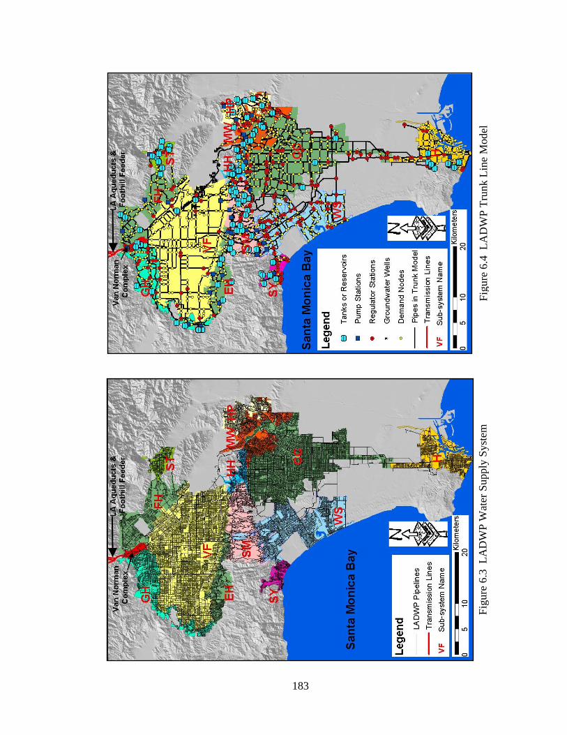
183

Figu

re 6

.3 L

AD

WP

Wat

er S

uppl

y Sy

stem

Fi

gure

6.4

LA

DW

P Tr

unk

Line

Mod

el

184

Monica Mountains (SM), Hollywood Hills (HH), Westside (WS), Santa Ynez (SY),

Mountain Washington (MW), Highland Park (HP), Central City (CC), and Harbor (H).

Among the 13 subsystems, the VF and CC are the two largest, serving the heavily

populated San Fernando Valley and Los Angeles central city. The other 11

subsystems are distributed around these two large subsystems. To accommodate

elevation variations and keep water pressure at acceptable levels, each subsystem is

further divided into several pressure zones. In total, the LADWP system includes 106

pressure zones. The pressure zone is named after the highest hydraulic grade, the sum

of elevation and pressure heads, in the zone. For example, pressure zone 1000 means

the highest hydraulic grade in this zone is 1000 ft (330 m). Wang (2006) provides a

detailed description of the LADWP water supply system.

6.3.2 LADWP Trunk System Model

To simulate system response under different operational scenarios, LADWP

developed a system-wide hydraulic network model. This model is used for planning

and operational purposes by LADWP and works with the software H2ONET

(LADWP, 2002), which is a member of the EPANET family. The major features of

H2ONET are discussed in Section 2.6.2. The H2ONET hydraulic network model is

shown in Figure 6.4. It includes 2186 km of pipelines with diameters generally larger

than or equal to 300 mm (12 in.). Some smaller diameter distribution lines are also

included in the model. The remaining 9800 km of distribution lines are modeled as

demand nodes shown as yellow dots in Figure 6.4. The network also includes 230

regulator stations, 110 tanks and reservoirs, 151 local groundwater wells, and 73 pump

stations. There are 591 valves set to control water flow and pressure in the 230

regulator stations, including 498 pressure reducing valves, 45 flow control valves, 50

185

throttle control valves, and 8 user defined valves. In general, multiple valves are set in

one regulator station to either control water flows in different pipes or serve as standby

valves to increase the reliability of the regulator station. There are 284 pumps at the

73 pump stations. Each local groundwater well is equipped with a pump for extracting

water.

Six different sets of demand are defined in the database, which are demands

for a typical winter day, a typical summer day, an ultimate summer day, the 1998

maximum day, a historical maximum day, and an ultimate maximum day. These

demand sets are defined by LADWP for planning and operational purposes.

This trunk system model is able to simulate performance throughout the

LADWP system or parts of the system, such as the 6 subsystems (subsystem VF, GH,

FH, EH, ST, and SM) in the San Fernando Valley. When modeling part of the system,

some virtual components are added to model other parts of the network that are

outside the model in terms of input-output relationships. For example, if the part of

system being modeled supplies water to other parts of the system, then a virtual

demand is added at the boundary of the model to represent water outflow.

6.3.3 LADWP Distribution System Models

In addition to the trunk system model, LADWP developed roughly 30

distribution system models. These local distribution models are pressure zone based.

For relatively large pressure zones, they are modeled as one distribution network

model. For relatively small pressure zones, they are combined into one distribution

network model. The smallest diameters of pipelines in these distribution network

186

models are 100 (4) and 150 mm (6 in.). The majority of pipelines in the distribution

networks has diameters smaller than or equal to 300 mm (12 in.). Appendix A

provides a pie chart showing the pipe diameter distribution of each distribution

network.

Six representative distribution network models were obtained from LADWP.

Five of them, systems 1449, 1000, 579, 448 & 462, and 426 were used to develop

fragility curves for earthquake demand simulations. Fragility curves developed from

Monte Carlo simulations from the five distribution networks were used to predict

performance in the sixth distribution network, and the prediction was compared with

the results of simulations performed explicitly with the hydraulic model for the sixth

network.

A map showing the locations of the six distribution systems is provided in

Figure 6.5. The distribution systems 1449, 1000, 579, and 205 cover the pressure

zones 1449, 1000, 579, and 205, respectively. System 448 & 462 combines the two

pressure zones, 448 and 462, because they are located close to each other. System 426

includes pressure zone 426 and the two small zones, 405 and 420. Appendix A

provides an expanded view of each distribution network.

The five distribution systems used to develop the fragility curves were

carefully selected from the 30 distribution system models developed by LADWP

according to the following criteria: 1) widely distributed throughout the LADWP area,

2) representative of different network topologies, 3) representative of different

pressure levels, and 4) reasonable size. System 1449 is located in the hillside area in

the northeast of San Fernando Valley with a very high mean pressure of 820 kPa (119

187

Figure 6.5 Locations of the Six LADWP Distribution Systems

188

psi). System 1000 is located in a flat area in the southern San Fernando Valley with a

mean pressure of 786 kPa (114 psi). Systems 579 and 448 & 462 are located in the

northeast portion of the Los Angeles central city with half hillside and flat areas and a

mean pressure of 655 (95) and 572 kPa (83 psi), respectively. System 426 is located

in the flat area in the northwest portion of the Los Angeles central city with a 427 kPa

(62 psi) mean pressure. The mean pressures of the five distribution networks range

from 427 (62) to 820 kPa (119 psi), which approximately covers the range of the mean

pressures in the entire LADWP system. In general, there are 130 to 200 km of

pipelines in each distribution network model.

6.4 DISTRIBUTION NETWORK SIMULATIONS

This section focuses on distribution network simulations and the development

of fragility curves for the assessment of earthquake demands in the trunk line model.

6.4.1 Simulation Procedures

The distribution network models include a limited number of large diameter

trunk lines as well as many small diameter distribution lines. In distribution system

simulations, pipe damage is evaluated only in the distribution lines since the trunk line

damage is accounted for explicitly in the trunk system model. This simulation

technique decouples damage to trunk and distribution systems. This decoupling

technique slightly overestimates water loss due to simultaneous damage in both the

trunk and distribution systems because water losses from distribution pipeline damage

are not diminished by trunk line losses. This modeling approach therefore provides a

conservative assessment of system serviceability. The conservatism is limited because

189

damage in the trunk system is relatively infrequent due to the comparatively small

number of trunk lines in the distribution network models.

The distribution network simulations are performed by GIRAFFE, standing for

Graphical Iterative Response Analysis for Flow Following Earthquakes. GIRAFFE is

a hydraulic network analysis software package, equipped with the algorithms for

negative pressure treatment and pipeline damage simulation, described in Chapters 3

and 5. The general procedure for simulations using GIRAFFE is to represent system

damage first, then solve for flow and pressure conditions in the damaged system,

followed by the iterative negative pressure elimination process. The salient features of

GIRAFFE are described in Chapter 7.

To simulate the distribution system damage, all distribution lines are assumed

to have an identical mean repair rate because the distribution model covers a relatively

small area in which the spatial variability of seismic hazard parameters is limited. The

locations of damage are generated using Monte Carlo simulations, as described in

Section 5.6.2.

Pipeline damage is classified as breaks or leaks using the assumption adopted

in HAZUS (NIBS, 1997) that 80% of earthquake damage occurs as leaks and 20%

occurs as breaks under the transient ground deformation effects. These percentages

are close to those applied by Ballantyne et al. (1990) and Hwang et al. (1998), who

assumed 15% is breaks and 85% is leaks for PGV-related damage to cast iron

pipelines.

190

To decide on the leak orifice area for leakage simulation, pipe material

information is needed. The LADWP distribution system database developed at

Cornell University was used for this information. The Cornell database was

developed by digitizing analogue maps of the LADWP system, which includes

roughly 11,000 km of distribution lines. Toprak (1999) and Jeon (2002) provide a

detailed description of the database. The statistics on pipeline composition show that

the majority of distribution lines are composed of cast iron. The percentage of cast

iron pipelines for distribution networks 1449, 1000, 579, 448 & 462, and 426, is 82%,

91%, 88%, 85%, and 83%, respectively. To simplify the simulation, it is assumed all

distribution pipelines are composed of cast iron. Linear regressions between

earthquake-induced pipeline repair rates and various seismic hazards including PGV

(O’Rourke and Toprak, 1997; Jeon and O’Rourke, 2005) for different types of

pipelines, show that the regressions for cast iron pipelines provide, in general, a

relationship that is consistent and slightly conservative with respect to those of other

distribution lines.

For cast iron pipelines, four leak scenarios are possible, which are annular

disengagement, round crack, longitudinal crack, and local loss of pipe wall. The

relative percentages of the four leak scenarios are 30%, 50%, 10%, and 10%,

respectively, as described in Chapter 5. For each leak, a uniformly distributed random

number between 0 and 1 is generated. If the random variable is within 0 to 0.3, the

leak is assigned as an annular disengagement; 0.3 to 0.8, round crack; 0.8 to 0.9,

longitudinal crack; and 0.9 to 1, local loss of pipe wall. The equivalent leak orifice

area is calculated using the equations developed in Section 5.4.4 and the damage to

each pipe is then added into the network.

191

Hydraulic network analysis was performed for the damaged system using

GIRAFFE, which uses the EPANET engine to solve flow equations with the iterative

approach, described in Chapter 3, to eliminate negative pressures. Flows in

representative trunk lines before and after damage to distribution lines were monitored,

and the flows after damage were normalized with respect to those before damage.

Because hydraulic network analysis solves the continuity equation with nodal

demands as input parameters, it is unable to track directly the variation of nodal

demands during the simulation. Flows in trunk lines were therefore used as a proxy

for the demands because water in the trunk lines is directly related to the nodal

demands. The monitored flows in each distribution network are shown in Appendix A.

6.4.2 Simulation Results

Monte Carlo simulations were performed for repair rates (RRs) ranging from

0.02 to 100. It is of no practical significance to model pipeline damage with an RR

lower than 0.02, which means, on average, one location of damage in 50 km of

pipelines. Previous research (Jeon, 2002) shows that RR equal to 1 repair/km provides

an approximate upper bound for the PGV-related damage to buried pipelines. RR of 1

to 100 repairs/km represents a level of damage that exceeds most levels of earthquake

related pipeline damage, except for those in areas of very large, highly localized

permanent ground deformation.

Figures 6.6 and 6.7 show simulation results of normalized demand (ND) vs RR

corresponding to different RR ranges for Pipes 9 and 5 in distribution network 1449.

Normalized demand is defined as the ratio of demand from a distribution network after

damage to demand before damage. These figures show that the relationships between

192

Pipe 9

0

1

2

3

4

5

6

7

0 0.2 0.4 0.6 0.8 1

Repair Rate (No/km)

Nor

mal

ized

Dem

and

a) RR Ranging from 0 to 1 Repairs/km

Pipe 9

0

1

2

3

4

5

6

7

0 2 4 6 8 10

Repair Rate (No/km)

Nor

mal

ized

Dem

and

b) RR Ranging from 0 to 10 Repairs/km

Pipe 9

0

1

2

3

4

5

6

7

0 20 40 60 80 100

Repair Rate (No/km)

Nor

mal

ized

Dem

and

c) RR Ranging from 0 to 100 Repairs/km

Figure 6.6 ND vs. RR Relationship for Various Damage States for Pipe 9

Separation of ND for Very Heavily Damage States

Separation of ND for Heavily Damage States

SI

Y= 1.7837*X +1.1685 r2 = 0.73

Linear trend for RR smaller than 2 repairs/km

193

Pipe 5

0

1

2

3

4

5

0 0.2 0.4 0.6 0.8 1

Repair Rate (No/km)

Nor

mal

ized

Dem

and

a) RR Ranging from 0 to 1 Repairs/km Pipe 5

0

1

2

3

4

5

0 2 4 6 8 10

Repair Rate (No/km)

Nor

mal

ized

Dem

and

b) RR Ranging from 0 to 10 Repairs/km

Pipe 5

0

1

2

3

4

5

0 20 40 60 80 100

Repair Rate (No/km)

Nor

mal

ized

Dem

and

c) RR Ranging from 0 to 100 Repairs/km

Figure 6.7 ND vs. RR Relationship for Various Damage States for Pipe 5

S

Y= 2.0527*X +1.2542 r2 = 0.78

I

Separation of ND for Heavily Damage States

ND Drops for Very Heavily Damage States

194

ND and RR follow increasing trends to RR of roughly 2 repairs/km, above which a

change in performance can be discerned. When RR values are 2 to 10 repairs/km, ND

begins to separate into different trends. At RR from 10 to 100 repairs/km, the system

response follows a limited number of discrete trends, and in some cases ND drops to

very low levels, which indicate that the system is severely damaged and not able to

supply water in a reliable and stable way.

Since RR equal to 1 repair/km provides an approximate upper bound for the

PGV-related damage to buried pipelines, statistics were developed for simulation

results with RR ranging from 0.02 to 1 repairs/km. The number of Monte Carlo

simulations was automatically determined by the GIRAFFE self-termination algorithm.

GIRAFFE monitors the mean and coefficient of variation (COV) of ND, as the

number of Monte Carlo simulations increases. If the mean and COV of ND with

additional simulations are within 2% difference when compared with those without

additional simulations, GIRAFFE terminates the Monte Carlo simulations.

Various types of regression functions were used to correlate ND and RR.

Linear regressions were found to provide correlations with highest statistical

significance between ND and RR. The linear regressions between ND and RR for the

26 monitored pipes for damage states with RR ranging from 0.02 to 1 repairs/km are

presented in Appendix B.

Figure 6.8 summarizes the linear regressions for the 26 locations in the five

distribution networks where flows were monitored before and after the simulation of

damage states. Table 6.1 provides a summary for the pipelines that served as

monitoring stations, including the ID (identification number) of the monitored pipeline

195

0

1

2

3

4

5

6

0 0.2 0.4 0.6 0.8 1

Repair Rate (RR, No/km)

Nor

mal

ized

Dem

and

(ND

)

0

1

2

3

4

5

6System 1449 [820 kPa (119 psi)]System 1000 [786 kPa (114 psi)]System 579 [655 kPa (95 psi)]System 426 [572 kPa (83 psi)]System 448 & 462 [427 kPa (62 psi)]

Figure 6.8 Relationship Between Normalized Demand and Repair Rate

in the hydraulic network database, pipe diameter, original flow rate, as well as slope

and intercept of the linear regression pertaining to each monitoring location. The

mean and standard deviation of the slopes and intercepts for the regressions associated

with each distribution network, together with the mean pressure (MP) of that

distribution network, are listed in Table 6.1. The MP is the average of nodal pressures

in the distribution network. Water loss caused by pipe damage, including both leaks

and breaks, is a function of pipe internal pressure. The MP, therefore, is an important

parameter for characterizing water loss in damaged pipeline networks.

6.4.3 Fragility Curve Construction

Since linear regressions provide the most statistically significant correlation

between ND and RR, a linear function is proposed to relate ND to RR as

Tabl

e 6.

1 S

imul

atio

n R

esul

ts fo

r Fiv

e R

epre

sent

ativ

e D

istri

butio

n N

etw

orks

in L

AD

WP

Syst

em

Zone

N

o.

Mea

n Pr

essu

re

Pipe

ID

Pi

pe D

iam

eter

Initi

al F

low

Slop

e M

ean

Slop

e Sl

ope

STD

* In

terc

ept

Mea

n In

terc

ept

Inte

rcep

t ST

D*

kPa

psi

mm

(in

.) (L

/s)

(gpm

)

1449

82

0 11

9

4 91

4 36

81

0 12

845

3.37

2.20

0.

92

1.66

1.28

0.

20

161

406

16

82

1299

3.

19

1.44

40

76

2 30

19

4 30

72

2.73

1.

24

5 10

67

42

581

9214

2.

05

1.25

9

1524

60

84

0 13

322

1.78

1.

17

2 91

4 36

61

0 96

73

1.15

1.

11

21

914

36

954

1511

6 1.

13

1.10

1000

78

6 11

4

88

305

12

63

1002

2.

34

1.82

0.

60

1.26

1.41

0.

12

87

356

14

144

2288

2.

31

1.56

17

8 30

5 12

82

12

98

1.47

1.

43

153

305

12

147

2324

1.

15

1.38

579

655

95

366

305

12

97

1534

2.

10

1.54

0.

56

1.27

1.21

0.

06

38

914

36

395

6260

1.

92

1.27

48

3 25

40

100

1902

30

152

1.21

1.

17

227

610

24

407

6455

0.

92

1.15

426

572

83

64

406

16

276

4368

1.

49

1.05

0.

26

1.28

1.15

0.

12

3 30

5 12

77

12

26

1.19

1.

00

176

305

12

144

2287

1.

05

1.26

5

610

24

525

8326

0.

97

1.02

12

4 40

6 16

21

8 34

61

0.87

1.

22

1 76

2 30

73

7 11

682

0.74

1.

09

448

&

46

2 42

7 62

41

1067

42

58

8 93

16

1.09

0.72

0.

34

1.24

1.16

0.

08

140

1016

40

80

1 12

694

0.87

1.

21

42

610

24

168

2667

0.

82

1.17

37

61

0 24

16

4 25

94

0.65

1.

15

1 10

67

42

806

1277

7 0.

19

1.02

* S

TD: S

tand

ard

Dev

iatio

n

196

197

RRSIND *+= (6.1)

in which ND is the normalized demand, I and S are the intercept and slope of the

regression, respectively, and RR is the repair rate. The RR, in turn, is correlated with

peak ground velocity. Equation 6.1 relates the distribution network damage states to

seismic hazard intensity, and provides the basis for generating fragility curves for

distribution system performance.

6.4.3.1 Observations

Figure 6.8 and Table 6.1 show that there are significant differences among the

different regressions. In general, the regression lines from distribution systems with a

relatively high MP are higher than those from distribution systems with a relatively

low MP. The highest regression lines are from System 1449, which has the highest

MP of 820 kPa (119 psi). The lowest regression lines are from System 448 & 462,

which has the lowest MP = 427 kPa (62 psi). The regression lines from other

distribution systems lie between those with the highest and lowest MPs and increase

with increasing MP.

To show how ND varies as MP, the slope and intercept of the linear regression

of ND vs RR for each monitoring location in each distribution network is plotted vs

MP in Figures 6.9 and 6.10, respectively. The intention of monitoring flows at

specific locations throughout a distribution network is to estimate the expected

demand of that distribution network on the trunk line system. The expected nodal

demand is estimated by determining the mean slope and intercept associated with the

linear regressions of ND vs RR for the multiple sampling locations in each distribution

198

0

1

2

3

4

400 500 600 700 800

Mean Pressure

Slop

e

0

1

2

3

458 68 78 88 98 108 118 (psi)

System 448 & 462System 426System 579System 1000System 1449

(kPa)

Figure 6.9 Regression Relationship Between Mean Pressure and Slope

0.0

0.3

0.6

0.9

1.2

1.5

1.8

400 500 600 700 800Mean Pressure

Inte

rcep

t

0.0

0.3

0.6

0.9

1.2

1.5

1.858 68 78 88 98 108 118

System 448 & 462System 426System 579System 1000System 1449

(psi)

(kPa)

Figure 6.10 Regression Relationship Between Mean Pressure and Intercept

199

network. The mean slopes and intercepts are plotted vs MP in Figures 6.11 and 6.12,

respectively. The high r2 values associated with these plots show that the variation of

the mean values, and hence estimate of nodal demands, is well explained by the

regression equations.

The variability of flows sampled at different locations should also be correlated

with MP because higher pressures will tend to drive higher water losses in a damaged

network. To estimate the variability of the estimated NDs with respect to MP, the

standard deviations of the slopes and intercepts associated with the ND vs RR

regressions are plotted in Figures 6.13 and 6.14.

6.4.3.2 Mean Regression with Noise Term

In this section, a linear regression with a noise term is proposed to estimate the

slope and intercept of ND vs RR relationship. The mean slope and intercept are

linearly correlated with MP, while a noise term is used to express the variability of the

slope and intercept. The noise term is modeled as a Gaussian random variable with

zero mean and variance, which is correlated with MP.

Using the mean regression with noise term, the slope, S, of the correlation

between ND and RR, is estimated as

),0(0248.0877.0),0( SS NMPNMPSSSIS σσ ++−=+×+= (6.2)

where SI and SS are the intercept and slope of the slope term, S, and ),0( SN σ is a

Gaussian random variable with zero mean and standard deviation Sσ . The values of

200

y = 0.0248x - 0.877r2 = 0.9608

0.0

0.5

1.0

1.5

2.0

2.5

400 500 600 700 800

Mean Pressure

Mea

n of

Slo

pe

0.0

0.5

1.0

1.5

2.0

2.558 68 78 88 98 108 118 (psi)

DataLinear (Data)

(kPa)

Figure 6.11 Regression Relationship Between Mean Pressure and Mean Slope

y = 0.0036x + 0.9012r2 = 0.6187

0

0.3

0.6

0.9

1.2

1.5

1.8

400 500 600 700 800Mean Pressure

Mea

n of

Inte

rcep

t

0.0

0.3

0.6

0.9

1.2

1.5

1.858 68 78 88 98 108 118

DataLinear (Data)

(psi)

(kPa)

Figure 6.12 Regression Relationship Between Mean Pressure and Mean Intercept

201

y = 0.0094x - 0.351r2 = 0.7189

0.0

0.2

0.4

0.6

0.8

1.0

400 500 600 700 800

Mean Pressure

STD

of S

lope

0

0.2

0.4

0.6

0.8

158 68 78 88 98 108 118 (psi)

DataLinear (Data)

(kPa)

Figure 6.13 Regression Relationship Between Mean Pressure and Standard Deviation

of Slopes

y = 0.0015x - 0.0198r2 = 0.4347

0.00

0.05

0.10

0.15

0.20

0.25

0.30

400 500 600 700 800Mean Pressure

STD

of

Inte

rcep

t

0.00

0.05

0.10

0.15

0.20

0.25

0.3058 68 78 88 98 108 118

DataLinear (Data)

(kPa)

(psi)

Figure 6.14 Regression Relationship Between Mean Pressure and Standard Deviation

of Intercepts

202

SI and SS are determined from the regression equation shown in Figure 6.11. The

value of sσ is evaluated using the regression equation shown in Figure 6.13.

3510.00094.0 −=×+= MPMPSSDISDSσ (6.3)

where the ISD and SSD are the intercept and slope of the linear regression between the

standard deviation of the slope term, S, and MP.

Similarly, the intercept, I, of the correlation between ND and RR is estimated

as

),0(0036.09012.0),0( II NMPNMPISIII σσ ++=+×+= (6.4)

in which, II and IS are the intercept and slope of the intercept term, I, and ),0( IN σ is

a Gaussian random variable with zero mean and standard deviation of Iσ . The values

of II and IS are determined from the regression equation shown in Figure 6.12. The

value of Iσ is evaluated using the regression equation shown in Figure 6.14 as

0198.00015.0 −=×+= MPMPISDIIDIσ (6.5)

where the IID and ISD are the intercept and slope of the linear regression between the

standard deviation of the intercept term, I, and MP.

Substituting Equations 6.2 to 6.5 into 6.1, ND can be estimated as a function of

RR and MP with the following equation

203

[ ] [ ][ ]{ }[ ]{ }RRMPNMP

MPNMPRRNMPSSSINMPISII

RRSIND

SI

)0094.0351.0( ,00248.0877.0 )0015.00198.0( ,00036.09012.0

),0(),0(

+−++−++−++=

×+×+++×+=×+=

σσ (6.6)

Please note that all the above regressions are performed with MP in the units of

psi. When applying Equation 6.6 to predict NDs, the MP needs to be converted into

the units of psi. The MP is influenced by the physical and operational properties of

the water supply network, and the RR is related to seismic hazard parameters.

Equation 6.6 correlates the mean slope and intercept of ND vs RR regressions with MP,

and characterizes the variability of slope and intercept.

Statistically Equation 6.6 can provide an accurate prediction of mean NDs over

a large area, and therefore may be more suitable for regional economic impact

assessments. With Equation 6.6, however, it is possible to underestimate ND, and

therefore overestimate the serviceability, with 50% chance for each individual demand

node. This is because the variation of the slope and intercept, associated with the

linear regression of ND vs RR, with respect to the mean value is simulated as a

Gaussian random variable with 0 mean. For each individual demand node, the

predicted slope and intercept, and therefore ND, may be lower than their expected

values with a probability of 0.5. With the increase of the number of demand nodes,

the average of slopes and intercepts, and therefore NDs, for all the nodes will

converge to their expected values.

It is useful to provide a conservative estimate of the NDs for emergency

situation simulations, such as fire emergency response. An appropriately conservative

estimate may be taken at the 90% confidence level, as explained in the next subsection.

204

6.4.3.3 90% Confidence Level Regression

In Equation 6.6, the parameters, II, IS, SI, SS, are mean estimates. Using the

26 locations, the confidence intervals of these parameters can be estimated. The

methodology for estimating the confidence intervals of the parameters of a linear

regression from experimental data can be found in traditional text books on statistics

(e.g., Ronald, et al., 1998) and the confidence intervals can be estimated using the

Regression Function under the Data Analysis menu in Microsoft EXCEL.

Selecting the Mean Pressure column in Table 6.1 as X and the Slope column in

Table 6.1 as Y, the 90% confidence intervals of the regression parameters, SI and SS,

for the slope term, S, are calculated as

0347.001640.0 ≤≤ SS (6.7)

0514.08433.1 −≤≤− SI (6.8)

Similarly, the 90% confidence intervals of II and IS are calculated as

0055.00010.0 ≤≤ IS (6.9)

1412.17017.0 ≤≤ II (6.10)

Because the purpose of using the confidence estimates is to provide a

conservative estimate, the lower confidence estimates do not have practical

significance. Only the upper 90% confidence estimates are used. The 90%

confidence limit of the slope, S, can be estimated as

205

MPMPSSSIS ×+−=×+= 0347.00514.0 (6.11)

and the 90% confidence limit of the intercept, I, can be estimated as

MPMPISIII ×+=×+= 0055.01412.1 (6.12)

Therefore, the 90% confidence level of ND as a function of RR and MP can be

expressed as

[ ] [ ]( ) ( )RRMPMP

RRMPSSSIMPISIIRRSIND

0347.00514.00055.01412.1

+−++=××++×+=

×+= (6.13)

6.4.4 Test of Fragility Curves

To test the predictive capabilities of the fragility curves, they were used to

predict performance of a sixth distribution network, and the predictions were

compared with the results of simulations performed explicitly with the hydraulic

model for the sixth network. The sixth distribution network covers pressure zone 205

in the LADWP system. A map of this local distribution network superimposed on the

trunk line network is shown in Appendix A. The same Monte Carlo procedures as

described in Section 6.4.1 were applied during the System 205 simulation. The

detailed simulation results are shown in Appendix B.

The mean pressure of System 205 is 490 kPa (71 psi), as determined by

averaging its nodal pressures in an undamaged state. The mean and 90% confidence

levels of the ND vs RR are plotted in Figure 6.15 by substituting the MP = 71 psi

206

0

1

2

3

4

5

6

0 0.2 0.4 0.6 0.8 1

Repair Rate (RR, No/km)

Nor

mal

ized

Dem

and

(ND

)

Mean Estimate90% Confidence Level EstimateTheoretical Lower BoundPipe 6 (y=2.3938x+1.2785, r^2=0.77)Pipe 457 (y=2.3288x+1.3941, r^2=0.72)Pipe 274 (y=1.9194x+1.1902, r^2=0.52)Pipe 244 (y=1.6626x+1.4347, R^2=0.64)Pipe 3 (y=1.4795x+1.2579, r^2=0.78)Pipe 560 (y=1.2676x+1.1630,r^2=0.49)

Figure 6.15 Comparison Between Simulated and Predicted Results for Distribution

System 205

(490 kPa) into Equations 6.6 and 6.13, respectively. Furthermore, the lower bound of

ND =1 is also shown in Figure 6.15 for reference. The linear regressions of ND vs RR

from simulation results at 6 monitoring locations are also plotted in Figure 6.15.

Figure 6.15 shows that the simulation results lie between the mean and 90%

confidence level predictions. Although the simulation results plot above the mean

regression, they all fall well within the 90% confidence level, suggesting that a 90%

confidence margin is appropriate for predicting local distribution network performance.

The characteristics of System 205 deserve some commentary. As shown in

Figure 6.5, System 205 is at the end of the trunk line flow paths, and is the only

network so located that was evaluated in this work. Water flow cannot by-pass

207

damage in the System 205 pipelines that are downstream of all trunk line sources. As

a result, the flows and losses in System 205 tend to be relatively larger than those in

distribution networks with both upstream and downstream trunk line interconnections.

In addition, the percentage of distribution pipelines is larger in System 205 than in

other local distribution networks studied because it has fewer trunk lines integrated

within it. This bias tends to generate additional break and leak locations in the local

network, which affects a smaller aggregate length of trunk lines. The ND, which is

evaluated from monitoring points in the smaller length of trunk lines, will be weighted

to reflect greater losses per level of repair rate.

209

CHAPTER 7

EVALUATION OF NORTHRIDGE EARTHQUAKE

PERFORMANCE

7.1 INTRODUCTION

To implement the modeling methodology, as described in Chapters 3, 5, and 6,

a software package, GIRAFFE, was developed for hydraulic network analyses of

heavily damaged water supply systems. GIRAFFE, standing for Graphical Iterative

Response Analysis for Flow Following Earthquakes, has special features to treat

negative pressures, simulate various levels of leakage, assess earthquake demand

associated with distribution networks, and perform Monte Carlo simulations.

To assess the capabilities of GIRAFFE, the response of the LADWP water

supply to the Northridge earthquake is used to compare the actual measured flows in a

heavily damaged system with earthquake simulation results. To monitor network

performance, the LADWP operates a Supervisory Control and Data Acquisition

(SCADA) system. The records of flow meters at key locations in the LADWP system

before and after the Northridge earthquake were collected and compared with the

GIRAFFE simulation results.

This chapter starts with a description of the software package GIRAFFE. It

then proceeds to the observed performance of the LADWP system during the 1994

Northridge earthquake, followed by the GIRAFFE simulation of the LADWP system

210

response to the Northridge earthquake, and comparisons between simulated and

observed performance.

7.2 GIRAFFE

A software package, GIRAFFE, was developed to help implement the

modeling approaches proposed in this study. GIRAFFE embodies an iterative

procedure for negative pressure elimination as described in Chapter 3, methods for

simulating pipeline breaks and leaks as described in Chapter 5, and the simulation of

earthquake demands associated with distribution networks as explained in Chapter 6.

GIRAFFE involves over 7000 lines of C++ code and works iteratively with the

EPANET hydraulic network analysis engine. GIRAFFE can perform both

deterministic and probabilistic simulations, and provides results which can be directly

linked to GIS to conduct spatial analysis and map presentations.

A complete GIRAFFE package consists of an EPANET graphical user

interface, an EPANET hydraulic analysis engine, and a GIRAFFE core code. The

GIRAFFE package includes six major modules, which are system definition, system

modification, seismic damage, earthquake demand simulation, hydraulic network

analysis, and compilation of results. A flow chat of GIRAFFE simulation is shown in

Figure 7.1. The major functions of each module are introduced in the following

sections.

211

Defining a water system

Editing the water system

Simulating earthquake demand

Performing hydraulic analysis using EPANET

Connectivity error?

Yes Modifying the water system

Pi < Plimit exists for any node i?

No

Yes

Assessing EPANET results

No

Compiling final results

Figure 7.1 GIRAFFE Simulation Flow Chart

Preprocessor

Postprocessor

Damaging the water system

Analysis

212

7.2.1 System Definition

The system definition module defines the hydraulic network being analyzed. It

provides information on the physical and operational properties, topology, and

demands of a system. The detailed information needed for defining a hydraulic

network is described in Chapter 2. GIRAFFE utilizes the graphical user interface of

EPANET for network definition and visualization. Users can refer to the EPANET

manual (Rossman, 2000) for the details on how to define a hydraulic network. The

system definition information from the graphical user interface is stored in a data file

with the format which can be read by EPANET engine. Users can also work with

other software packages, such as H2ONET, to define a hydraulic network and then

export the system definition file into the EPANET format. Because of the wide usage

of EPANET engine, most of the commercial software packages for hydraulic network

analysis can export their system definition files into the EPANET format. The

EPANET format serves as a common platform for data exchanges among different

hydraulic network analysis software packages.

7.2.2 System Modification

The system modification module is used to modify a hydraulic network to

perform a specific simulation scenario. Users can add or remove components and

change the physical and operational properties of components in the hydraulic network

model. Users can modify the system graphically using the EPANET graphical user

interface or modify the system definition data file directly.

213

7.2.3 System Damage

The damage module adds damage to pipelines. Algorithms for damage to

other components, such as tanks, pumps, and valves, can be incorporated in GIRAFFE

because the architecture of the code allows for the addition of parallel damage

characterization modules.

The detailed modeling methodology for pipe damage is described in Chapter 5.

In general, a break or leak can be modeled. For a pipe leak, there can be five different

scenarios, which are annular disengagement, round crack, longitudinal crack, local

loss of pipe wall, and local tear of pipe wall. One pipe can have multiple breaks and

leaks. Two simulation options, deterministic and probabilistic, are provided for pipe

damage.

7.2.3.1 Deterministic Simulation

The deterministic option allows users to specify the location of each break, and

the location and orifice area of each leak. The location of each break and leak is

characterized by a unique pipe ID and a length ratio. A length ratio is the relative

length, between the pipe upstream node and the damage location, with respect to the

pipe length. Each pipe is connected to upstream and downstream nodes that have geo-

coordinates. By knowing the pipe ID in which the damage occurs and the length ratio,

one can locate damage precisely. Multiple breaks or leaks in the same pipeline are

distinguished by different length ratios. All damage information is stored in an input

text file. The basic input parameters for a pipe break are the pipe ID and length ratio.

214

The basic input parameters for a pipe leak include the pipe ID, length ratio, and the

equivalent orifice diameter.

To model a pipe break, GIRAFFE modifies the system definition file by

deleting the original pipe according to its unique pipe ID and adding two new pipes

and two empty reservoirs following the method described in Section 5.5.

To model a pipe leak, GIRAFFE modifies the system definition file by: 1)

adding a new junction at the leak location to divide the original pipe into two new

pipes; 2) adding an empty reservoir which has the same elevation as the leak location;

3) and adding a new pipe with a length of 1 foot, roughness coefficient of 1,000,000,

and minor loss coefficient of 1 to connect the newly added junction and reservoir. The

leak simulation method is described in Section 5.4.

7.2.3.2 Probabilistic Simulation

The probabilistic option generates randomly distributed pipe breaks and leaks

according to repair rate, RR, pipe length, L, and conditional pipe break probability,

bkP , given that damage occurs. For each leak, the probabilistic simulation option

randomly generates the scenario of each leak and calculates the orifice area. The

probabilistic simulation of pipe damage includes three steps: generating pipe damage,

deciding the damage state as a leak or break, and deciding the scenario and orifice area

of each leak.

The basic input parameters for generating pipe damage are the mean repair rate,

RR, and length, L, of each pipeline. The repair rate, RR, is correlated with seismic

215

hazard parameters and is an input parameter for each pipe. The length, L, of each pipe

can be obtained from the hydraulic network database. The pipe damage is assumed to

follow a Poisson process with a mean arrival rate equal to mean repair rate, RR. For a

Poisson process, the arrival length between two locations of damage follows an

exponential distribution. By continually generating the damage arrival length using

Monte Carlo simulation until the cumulative length of the damage exceeds the

pipeline length, the locations of damage can be determined. The detailed Monte Carlo

simulation algorithm is described in Section 5.6.2.

After generating the locations of damage for each pipeline, another uniformly

distributed random number between 0 and 1 is generated for each location of damage.

This random number is compared with the conditional pipe break probability, bkP . If

the uniformly distributed random number is greater than the pipe break probability,

then the damage is classified as a leak, otherwise, it is a break. The pipe break

probability is an input parameter which is estimated from pipe damage data collected

from previous earthquakes.

To decide the leak orifice area, a uniformly distributed random number

between 0 and 1 is generated for each leak. This random number is compared with the

cumulative probability of each leak scenario for a pipeline with specific material

composition. The probabilities of each leak scenario for various types of pipelines

widely used in North American are listed in Table 5.2. The equivalent orifice area for

each leak is then calculated using equations developed in Section 5.4.4.

216

7.2.4 Earthquake Demand Simulation

The earthquake demand simulation module implicitly considers the effects of

damage to small diameter distribution pipelines, which are not included in the

hydraulic network model, by increasing nodal demands. The detailed modeling

methodology for earthquake demand simulation is provided in Chapter 6.

The earthquake demand simulation is pressure zone based. The basic input

parameters are mean pressure (MP) and repair rate (RR) associated with each demand

node. For a demand node, MP is the average nodal pressure in the pressure zone in

which the demand node is located before system damage. The MP can be obtained by

performing hydraulic network analysis on the undamaged system and then conducting

statistical analysis on the nodal pressures with respect to pressure zones. The RR

represents the repair rate of the distribution lines around the demand node. For PGV-

related pipe damage, the RR is calculated using regression relationships between PGV

and RR developed from previous investigations (e.g., Jeon, 2002; Jeon and O’Rourke,

2005). The determination of RR for a given earthquake scenario involves spatial

manipulation and is performed using GIS, which gives the RR related to each demand

node as input to GIRAFFE. The GIS procedures for determining the RR is explained

in Section 7.3.3.2 for the Northridge earthquake case history simulation.

Two implementation options are provided in GIRAFFE, mean prediction with

noise terms and 90% confidence level prediction. With the input MP and RR for each

demand node, GIRAFFE calculates the normalized demand using Equations 6.6 and

6.13 for mean and 90% confidence level predictions, respectively. The standard

normal random variables in Equation 6.6 are generated by the computer. GIRAFFE

217

then calculates the demands after the earthquake by multiplying the normalized

demands with the original demands, and modifies the system definition file by

replacing the original demands with the earthquake demands.

7.2.5 Hydraulic Network Analysis

This module uses the EPANET hydraulic network engine iteratively to solve

the damaged hydraulic network and eliminate negative pressures. Only steady state

simulation is performed. As shown in Figure 7.1, the damaged system is sent to

EPANET engine for hydraulic network analysis. It is possible that the damaged

system cannot be solved because some elements may not have connectivity with the

main system due to earthquake damage. In this case, the EPANET engine gives error

messages, which tell the user the ID of each element disconnected from the main

system. GIRAFFE reads the error messages and fixes the errors by eliminating the

disconnected elements from the database. GIRAFFE then checks the nodal pressures,

and identifies the lowest nodal pressure in the system. If the lowest pressure is higher

than the preset pressure limit, which is zero for negative pressure elimination, the

hydraulic analysis stops. If the lowest pressure is lower than the pressure limit, the

program eliminates the node, the links connected to this node, and other operational

parameters associated with the node and links. After each step of elimination,

GIRAFFE performs hydraulic network analysis again and this process continues until

there is no pressure lower than the pressure limit in the system. The reason to use a

pressure limit instead of zero is to increase the flexibility of the program. For

example, it can be used to identify the areas with inadequate pressures for fire fighting

by setting a pressure limit specified for fire fighting purposes.

218

7.2.6 Compilation of Results

This module compiles the hydraulic analysis results into the format compatible

with GIS. It also provides a performance index to measure the system serviceability.

7.2.6.1 Hydraulic Network Analysis Results

The final hydraulic analysis results are compiled such that they can be linked

to GIS. Because in GIS, junctions, pipes, pumps, valves, and tanks are different layers

which can be exported from the H2ONET LADWP model database, the hydraulic

analysis results are compiled for these five types of elements. Please note, reservoirs

are treated as a special type of tanks which have fixed grade. The major outputs for

pipes, valves, and pumps are the flow rate through them. The major outputs for

junctions and tanks are the pressure and grade at them. For the components that are

eliminated from the main system due to either negative pressure or connectivity

problems, their results are set to zero to represent the isolation of these components.

For deterministic simulation, the outputs for the five types of components are reported.

For probabilistic simulation, the outputs for the five types of components are reported

for the last run of the Monte Carlo simulation. The flow rates in pipes and pressures at

junctions, which are the key outputs, are reported for each Monte Carlo simulation

run. The mean, standard deviation, and coefficient of variation of the flow rate in each

pipe and pressure at each node for all Monte Carlo simulation runs are also calculated

and reported.

219

7.2.6.2 Performance Index

This module provides an index for measuring the seismic serviceability of a

damaged water supply system. The serviceability is defined as the ratio of the

available demand to required demand corresponding to a seismic damage scenario,

*T

Ts Q

QS = (7.1)

where sS is the serviceability, TQ is the available demand, and *TQ is the required

demand. The serviceability can be calculated for each demand node and for the entire

system. For deterministic simulation, the serviceability for each demand node is either

0, if this demand node is isolated due to the negative pressure or connectivity

problems, or 1, if this demand can be satisfied. The serviceability for the entire

system is the sum of the demands that can be satisfied over the sum of the total

required demands. For probabilistic simulation, the system serviceability is reported

in a matrix format. For each Monte Carlo simulation run, the serviceability is reported

for each demand node and for the entire system. The mean, standard deviation, and

coefficient of variation of the nodal and system serviceability for all Monte Carlo

simulation runs are also calculated and reported.

7.3 GIRAFFE SIMULATION OF NORTHRIDGE EARTHQUAKE

PERFORMANCE

To assess the capabilities of GIRAFFE, it was used to simulate the earthquake

response of the LADWP system to the Northridge earthquake. The water outages and

220

flows at key locations, simulated by GIRAFFE, were compared with the documented

water outages and flows measured by LADWP before and after the earthquake.

7.3.1 LADWP System Performance during Northridge Earthquake

The Northridge earthquake (Mw=6.7) struck Los Angeles at 4:30 a.m. local

time on January 17, 1994. The damage to water supply systems during the Northridge

earthquake is among the most extensive experienced in U.S. history, and is

comparable to the damage sustained during the 1906 San Francisco and 1971 San

Fernando earthquakes. The Northridge earthquake damaged 82 locations (Davis, 2003)

in trunk lines (pipe diameter ≥ 610 mm, 24 in.) and 1013 locations (Jeon, 2002) in

distribution lines (pipe diameter < 610 mm, 24 in.) in the LADWP system. Among

the 82 trunk line repairs, 70 occurred in the LADWP trunk lines and 12 occurred in the

trunk lines operated by Metropolitan Water District (MWD). The MWD trunk lines

are embedded in the LADWP system and do not supply water to the LADWP system

normally. Five water tanks in the LADWP system were also damaged.

Approximately 15% of the population in Los Angeles was subjected to water outages,

ranging from 1 to 7 days. Figure 7.2 shows the spatial distribution of the trunk line

repairs, distribution repairs (Jeon and O’Rourke, 2005), damaged tanks (Brown, et al.,

1995), and water outage areas (Lund et al., 2005) after the earthquake. Most locations

of the component damage and subsequent water outage areas were in San Fernando

Valley. The cost to repair the LADWP water supply system was about $44 million

(Eguchi and Chung, 1995; Tierney, 1997). The detailed performance of the LADWP

system during the Northridge earthquake is documented by Lund and Cooper (1995).

221

Figure 7.2 LADWP Damaged Tanks, Trunk and Distribution Line Repairs, and Water

Outage Areas after the Northridge Earthquake

222

7.3.2 LADWP Hydraulic Model for Northridge Earthquake

The multi-scale modeling technique developed in Chapter 6 is applied to

simulate the LADWP water supply response to the Northridge earthquake. This

technique simulates the trunk system response explicitly and simulates the distribution

system response implicitly by increasing nodal demands in the trunk system. The

LADWP system and the system-wide trunk system hydraulic model are described in

Sections 6.3.1 and 6.3.2, respectively. Figure 7.2 shows that more than 95% of trunk

line repairs, 80% of distribution repairs, all damaged tanks, and all water outages

occurred in San Fernando Valley. To simplify the simulation, only the response of the

LADWP system in San Fernando Valley, or northern half of the system, is simulated

explicitly. This southern half of the system is simulated as boundary conditions.

The northern half of the system consists of six subsystems: Granada Hills (GH),

Foothills (FH), Sunland/Tujunga (ST), Valley Floor (VF), Encino Hills (EH), and

Santa Monica Mountains (SM). The hydraulic model for these six subsystems is

called the Valley-Six submodel shown in Figure 7.3. The Valley-Six submodel

consists of 4674 links and 3878 nodes to model the 967 km of pipelines, 76 regulator

stations, 51 pump stations, 72 tanks and reservoirs, and 140 local groundwater wells.

There are 188 valves in the 76 regulator stations and 167 pumps in the 51 pump

stations. Each local groundwater well is equipped with a pump for extracting water.

There are 441 demand nodes distributed around the northern half of the system.

The majority of nodal demands are smaller than 63 liters per second (1000 gpm),

which are mostly consumed by local residents. A few nodal demands are higher than

63 liters per second (1000 gpm), and they are mainly related to industry usage. Three

223

Figure 7.3 LADWP Hydraulic Model for Northridge Earthquake Simulation

(1000 gpm = 63 L/s)

nodes, indicated as big red dots at Stone Canyon Reservoir Inlet, Upper Franklin

Reservoir Inflow, and River Supply Conduit in Figure 7.3, have a demand larger than

630 liters per second (10,000 gpm), which are virtual demands representing water

flow to the southern half of the system. Another connection between the Valley-Six

submodel and the southern half of the system is the Upper Hollywood Reservoir

Inflow, which is modeled as a virtual tank, representing water transportation to and

from the Upper Hollywood Reservoir. These virtual elements serve as the boundary

conditions for the Valley-Six submodel. The response of the Valley-Six subsystem

can be simulated after setting boundary conditions.

VF

GH

FH

EH

SM

ST

River Supply Conduit

Upper Hollywood Res. Inflow Upper Franklin

Res. Inflow

Stone Canyon Res. Inlet

224

7.3.3 Damage Simulation

To simulate the response of the Valley-Six subsystem, the damage to

components needs to be added into the model, followed by hydraulic network analysis

using GIRAFFE. The damage simulation is discussed in the following sections.

7.3.3.1 Trunk Line Damage

Because the MWD trunk lines did not supply water to the LADWP customers

during the Northridge earthquake, the 12 locations of damage in the MWD trunk lines

were not simulated. Among the 70 locations of LADWP trunk line damage, 67 are in

the trunk lines in the Valley-Six hydraulic model. One location is in the southern half

of the LADWP system. The other two locations are in the trunk lines, which are not

included in the hydraulic network model. These three locations were not simulated.

The detailed simulations of the 66 locations of LADWP trunk line damage are

described in Appendix C. In total, three breaks, in the Granada Trunk Line (GTL),

Rinaldi Trunk Line (RTL), and LA City Trunk Line, respectively, and 26 leaks were

simulated. The leaks were classified into five scenarios based on the damage

descriptions in Tables C1 to C5. The opening area of each leak was calculated using

the equations developed in Section 5.4.4. Multiple leaks, which are located close to

each other in the same pipeline, were simulated as one leak with an appropriately

increased orifice area. Leaks and breaks, which are located close to each other in the

same pipeline, were simulated as one break by disconnecting the pipeline completely.

225

7.3.3.2 Distribution Line Damage

Distribution lines account for the highest proportion of components in the

LADWP system, and suffered the most extensive damage during the 1994 Northridge

earthquake. A comprehensive GIS database, including information on distribution

pipeline length, composition, size, and repairs after the Northridge earthquake, was

developed by O’Rourke and Toprak (1997), O’Rourke et al. (1996), and Toprak

(1999). The total length of the LADWP distribution lines is about 10,750 km with

72% composed of cast iron. Most pipelines have a diameter of 150 mm (46%) or 200

mm (27%). There were 1,405 original repair records provided by LADWP. After a

careful evaluation of them, it was determined that 1,013 records were valid for damage

to distribution mains. It was further found that only 944 out of 1,013 repairs have pipe

composition and geodetic coordinates. The 944 repairs were used to develop the

regression relationships between RR and PGV for pipelines composed of different

materials. The procedures for developing the regressions are provided by Jeon (2002).

These regressions can be used to estimate the damage to distribution lines in future

earthquakes.

Since distribution lines are not modeled explicitly in the LADWP trunk model,

it is not able to model damage to distribution lines directly. To include the effects of

damage to distribution lines, the method developed in Chapter 6 is applied, in which

the distribution damage was implicitly modeled as increased demands at nodes in the

trunk system. To apply this method, the PGV contours, developed by Jeon (2002)

using the PGV recordings collected at 148 strong motion stations after the Northridge

earthquake, were used to obtain the PGV associated with each demand node. The

detailed procedures for generating the PGV contours are described by Jeon (2002).

226

When the PGV contour GIS and demand node GIS combined, the PGV in association

with each demand was determined. This PGV represents the PGV for the distribution

network around the demand node. The distribution network RR was then calculated

based on the linear regression relationship for cast iron pipelines developed by Jeon

(2002)

81.6)(21.1)( −= PGVLnRRLn (7.2)

Hydraulic network analysis was performed on the trunk model prior to

earthquake damage. The pressure was summarized for nodes in each pressure zone

and the mean pressure, MP, was calculated. The MP was assigned to each demand

node within the pressure zone. With the known mean pressure, MP, and repair rate,

RR, the normalized demand was calculated by

( ) ( )( ) ( ) RRMPMP

RRMPSSSIMPISIIRRSIND

××+−+×+=××++×+=

×+=

0248.0877.00036.09012.0 (7.3)

where all the symbols have the same meaning as those used in Equation 6.6 in Section

6.4.3.2. In contrast to Equation 6.6, which includes a noise term for slope, S, and

intercept, I, respectively, to model the uncertainties associated with normalized

demands, Equation 7.3 is deterministic for the Northridge earthquake scenario.

The distribution of normalized demands is shown in Figure 7.4. This figure

shows that the demands increase by 1 to 2.8 times the customer demand due to

damage to distribution lines during the Northridge earthquake. The nodes with the

highest normalized demand are located in the Van Norman Complex area, where the

227

Figure 7.4 Normalized Demands of Valley-Six Subsystem after Northridge

Earthquake

228

PGVs are the highest. In general, the normalized demands in mountainous areas are

higher than those in flat areas because the pipe internal pressure in mountainous areas

is higher than that in flat areas. The high variation of elevations in the mountainous

areas requires a high overall pressure to supply customers at multiple locations.

7.3.3.3 Tank Damage

In general, reservoirs and water tanks performed well during the Northridge

earthquake. Brown et al. (1995) summarized the performance of 65 LADWP tanks in

service at the time of earthquake (48 welded or riveted steel tanks and 17 reinforced

concrete or prestressed concrete tanks). Only 5 tanks were damaged. The damaged

tanks are indicated as pink symbols in Figure 7.5. Roof collapse and inlet/outlet pipe

damage occurred in the Coldwater Canyon, Beverly Glen, and Zelzah Tanks. The

Granada High Tank collapsed completely and was removed permanently from service

after the earthquake. Inlet/outlet pipe damage occurred to the Topanga Tank. Since

damage to all these tanks occurred to the inlet/outlet pipes, the inlet/outlet pipes were

disconnected in the hydraulic network simulation of post-earthquake performance.

The current LADWP trunk line model, which was used in this research, does not

include the Granada High Tank, and therefore, it was not simulated.

It was known through personal communications with LADWP engineers

(Vargas, 2005; Adams, 2005) that the Kittridge Tanks (including the Kittridge Tank

No 1 and 2) and De Soto Reservoir were depleted shortly after the earthquake. The

Kittridge Tanks are located along the western margin of San Fernando Valley and

supplied by the GTL. The broken section of the GTL cut off the water source to the

229

Figure 7.5 LADWP Tanks and Reservoirs, and Damaged Tanks

after Northridge Earthquake

Kittridge Tanks and was not able to refill them for over one week after their depletion.

The De Soto Reservoir is located along the northern margin of San Fernando Valley

and supplied by the RTL. The broken section of the RTL cut off the water source to

the De Soto Reservoir. The RTL was not able to refill the reservoir for over one week

after its depletion. Numerical simulation results showed that the Kittridge Tanks and

De Soto Reservoir would be depleted in about 2 and 1 hours after the earthquake,

respectively, if not refilled. To include the effects of the depletion of the Kittridge

Tanks and De Soto Reservoir, they were closed after the earthquake in the simulations.

230

7.3.3.4 Water-Electric Power Interaction

The interaction between water and electric power was accounted for in the

simulation. The Northridge earthquake caused a system-wide blackout of the

LADWP electric power system immediately after the earthquake, and it took from 1 to

27 hours to restore power (LADWP, 1994). The electric power outage affected the

operation of pump stations directly. The spatial distributions of pump stations and

electricity outage time are shown in Figure 7.6. A large portion of pump stations are

located around the Santa Monica Mountains, where the electricity outage time was

less than 8 hours. A small portion of pump stations are located in San Fernando

Valley, Granada Hills, Foothills, and Sunland/Tujunga, where the electricity outage

lasted for 15-27 hours. Generally, pump stations have diesel generators as backup

power. The performance of pump stations during previous natural disasters showed

that the diesel generators were able to generate enough power for the operation of

small pump stations, but not enough for large ones. The largest pump station, Van

Norman Pump Station No. 2, is located in the Van Norman Complex, where the

electricity outage lasted for the longest time. Accordingly, the Van Norman Pump

Station No. 2 was turned off in the hydraulic network simulation of post-earthquake

performance.

7.3.4 SCADA Data

To monitor network performance, the LADWP operates a Supervisory Control

and Data Acquisition (SCADA) system. The records of flow meters before and after

the earthquake in the northern half of the system were collected and reviewed. Due to

the earthquake damage and electricity outage, some of the SCADA data are not

231

Figure 7.6 Superposition of Spatial Distribution of Electricity Outage Time and Pump

Stations

232

reliable. A screening process was, therefore, conducted before utilizing the SCADA

data. Two screening criteria were adopted to assure the quality of the data: 1) the

meters indicating zero flow before and after the earthquake were considered to have

malfunctioned or have been out of service; and 2) the meters with a maximum

recorded flow smaller than 63 liters per second (1000 gpm) were not used because the

flows in such lines are too small and too sensitive to local variations in predicted

damage. Records at 13 locations were selected and utilized for three major purposes:

1) setting boundary conditions, 2) providing clues on system reconfiguration shortly

after the earthquake; and 3) comparing monitored and simulated flows.

7.3.4.1 Boundary Conditions

The four flow meter records at the River Supply Conduit, Upper Hollywood

Reservoir Inflow, Upper Franklin Reservoir Inflow, and Stone Canyon Reservoir Inlet,

which are indicated as red circles in Figure 7.7, were used to set boundary conditions.

The virtual demands at nodes for the River Supply Conduit, Upper Franklin Reservoir

Inflow, and Stone Canyon Reservoir Inlet, representing flows to the southern half of

the system, were recalibrated in accordance with the actual flow records at the three

locations before and after the earthquake, respectively. The virtual tank, Upper

Hollywood Reservoir, was changed to a virtual demand node and its demand was

calibrated in accordance with the actual flow records.

7.3.4.2 System Reconfiguration

Three flow meter records, at the LA City, Haskell, and Hayvenhurst Trunk

Lines in the lower Van Norman Complex, respectively, as illustrated by green squares

233

Figure 7.7 System Damage and SCADA Flow Meters

in Figure 7.7, were utilized to provide guidance on how the system was reconfigured

shortly after the earthquake. The three flow meter records showed that flows

decreased to zero shortly after the earthquake, indicating that local damage had been

isolated to curtail water losses. The isolated section of the LA City Trunk Line is

located upstream of its connection with the LA Reservoir Outlet, the main water

source to the LA City Trunk Line. Therefore, the isolation had little impact on the

water flow southward through the LA City Trunk Line.

234

7.3.4.3 Flow Comparison

Six SCADA flow meters records at the LA Reservoir Outlet, Encino Reservoir

outflow, Granada Trunk Line, Morella & Van Owen Regulator Station, Astoria Pump

Station, and Green Verdugo Pump Station, respectively, were used to compare the

measured flows and simulation results. The flow meters are shown as yellow triangles

in Figure 7.7.

7.3.5 Simulation Results

Since the Northridge earthquake occurred in January, a typical winter demand

was applied in the simulation. The Valley-Six hydraulic model was exported from

H2ONET software and imported into GIRAFFE. Component damage was then added

into the network model and hydraulic network analysis was performed. Figure 7.8

shows the GIRAFFE simulation results, superimposed by the observed water outages

(Lund et al., 2005). The original no-flow pipes in the intact system and the damage-

induced no-flow pipes are color coded by pink and red, respectively. The unsatisfied

demands, from which the customers should not receive water, are illustrated by yellow

dots. Most damage-induced no-flow pipes and unsatisfied demands are consistent with

the areas of observed water outage for 2 days or more. The water outages of less than

a day are related to temporary isolations that were restored after inspections revealed

no serious damage to local trunk lines.

Figure 7.9 shows detailed comparisons between GIRAFFE simulations and the

recorded flows. In general, the simulated flows compare favorably with the monitored

flows at each location.

235

Figure 7.8 GIRAFFE Simulation Results

Figure 7.9a shows that the monitored flows in the LA Reservoir Outlet varied

from 11,500 to 14,000 L/s depending on fluctuations in demand at different times of

the day. The flow reached its lowest value roughly at midnight and highest at 8 to 9

o’clock in the morning, reflecting the lowest and highest water consumptions at these

times. The steady state simulation shows that the flow rate in the LA Reservoir Outlet

prior to the earthquake was 12,100 L/s, which represents a rough average of the

monitored daily flows. The flow from the LA Reservoir increased to roughly 20,000

L/s shortly after the earthquake because of water losses from damage to major trunk

lines downstream of it. As discussed in Section 7.3.3.2, the LA City, Haskell, and

Hayvenhurst Trunk Lines, which are supplied by the LA Reservoir Outlet, sustained

236

5000

9000

13000

17000

21000

1/14/1994 1/16/1994 1/18/1994 1/20/1994Date

Flow

(L/s)

79252

129252

179252

229252

279252

329252

Flow

(gpm

)

Monitored DataSimulated Results

0

500

1000

1500

2000

2500

3000

1/14/1994 1/16/1994 1/18/1994 1/20/1994Date

Flow

(L/s)

0

10000

20000

30000

40000

Flow

(gpm

)


-100

100

300

500

700

1/14/1994 1/16/1994 1/18/1994 1/20/1994Date

Flow

(L/s)

-1585

1415

4415

7415

10415

Flow

(gpm

)


Figure 7.9 Comparisons Between GIRAFFE Results and Monitored Data

(e) Astoria Pump Station

(b) Encino Reservoir Outflow

(f) Green Verdugo Pump Station

(c) Granada Trunk Line Flow

(a) LA Reservoir Outlet

(d) Morella & Van Owen Regulator Station

-500

0

500

1000

1500

2000

2500

3000

1/14/1994 1/16/1994 1/18/1994 1/20/1994Date

Flow

(L/s

)

-7925

2075

12075

22075

32075

42075

Flow

(gpm

)


200

400

600

800

1000

1200

1/14/1994 1/16/1994 1/18/1994 1/20/1994Date

Flow

(L/s

)

3170

6170

9170

12170

15170

18170

Flow

(gpm

)


-100

0

100

200

300

400

500

1/14/1994 1/16/1994 1/18/1994 1/20/1994Date

Flow

(L/s

)

-1585

1415

4415

7415

Flow

(gpm

)


237

severe damage during the earthquake and were promptly isolated in the lower Van

Norman Complex after the earthquake to curtail water losses. After isolation, the flow

in the LA Reservoir Outlet dropped to between 10,000 and 12,500 L/s. The post-

earthquake simulation was performed after the isolation of the three pipe sections and

showed that the flow rate in the LA Reservoir Outlet is 10,500 L/s, which falls in the

range of monitored flows after the earthquake. Five days after the earthquake, flow in

the LA Reservoir Outlet decreased as repairs were undertaken in the LA aqueducts

and Van Norman Complex. Decreased flow related to system repairs was not

simulated.

Figure 7.9b shows that the monitored flows at the Encino Reservoir Outflow

station vary from 0 to 550 L/s depending on fluctuations in demand. The simulated

flow prior to earthquake is roughly 250 L/s, which lies in the range of the monitored

flows. The earthquake increased flows at the Encino Reservoir Outflow station

significantly. This is because the Encino Reservoir had to provide more water to the

southern part of San Fernando Valley after the earthquake to compensate the loss of

water sources, which are normally from the northern part of San Fernando Valley.

The post-earthquake simulated flow is 1600 L/s, which is within the range of

monitored flows, varying from 1500 to 2500 L/s.

Figure 7.9c shows that the Granada Trunk Line (GTL) supplies roughly 750 to

2500 L/s water to customers in normal situations. The simulated flow rate, 1750 L/s,

represents a rough average of the real flow rates. The earthquake ruptured the GTL

completely and resulted in zero simulated flow, which is consistent with the monitored

zero flow rate.

238

Figure 7.9d shows that roughly 400 to 900 L/s of water flows through the

Morella & Van Owen Regulator Station prior to earthquake. The simulated flow rate,

970 L/s, is approximately 10 % higher than the highest monitored flow. The water

source of the Morella & Van Owen Regulator Station is from local groundwater wells.

It is possible that LADWP uses more water from local groundwater wells in recent

years, which results in a higher flow through the Morella & Van Owen Regulator

Station than the monitored flows before the Northridge earthquake. After the

earthquake, the simulated flow drops to 550 L/s, which is roughly 10 % lower than the

monitored flow.

Figure 7.9e shows that the simulated flows vary from 0 to 300 L/s at Astoria

Pump Station, which matches the monitored flows very well. After the earthquake,

both the simulated and monitored flows at the Astoria Pump Station drop to zero. The

fluctuations of flow rates after January 19 might be associated with system repairs and

testing of the pump station. These fluctuations were not simulated in this study.

Figure 7.9f shows that the simulated and monitored water flows through the

Green Verdugo Pump Station are very consistent. The earthquake did not affect water

flows through the Green Verdugo Pump Station because it is located far away from

the system damage that occurred in the San Fernando Valley.

It should be noted that there are some differences between the 1994 system in

operation during the Northridge earthquake and the 2002 system represented by the

hydraulic network model. One example is the Granada High Tank, which collapsed

during the 1994 Northridge earthquake and was removed from the system. Also, the

239

demand used in the simulation is based on the typical winter demand used in the 2002

system model, which may slightly be different from the demand in January 1994.

In general, the GIRAFFE simulation compares favorably with the major

features of the observed response of the LADWP system during the 1994 Northridge

earthquake. The validated GIRAFFE was applied as a major tool for the seismic

performance evaluation of the LADWP system in conjunction with the state-of-the-art

seismic hazard characterization in the California area. The evaluation was conducted

by Wang (2006). In his study, the LADWP system response simulation was

performed for 59 earthquake scenarios and system serviceability risk curves were

constructed based on the simulation results. The simulation results and risk curves are

logic and being used for community restoration, emergency planning, and regional

economic impact assessments.

241

CHAPTER 8

SUMMARY AND CONCLUSIONS

8.1 INTRODUCTION

This report describes a comprehensive model for simulating the earthquake

performance of water supply systems. The model is developed in conjunction with the

water supply system operated by the Los Angeles Department of Water and Power

(LADWP). It includes an algorithm for the hydraulic network simulations of heavily

damaged water supply systems, an analytical model for analyzing seismic wave

interaction with underground water supply pipelines, methods for simulating pipeline

breaks and leaks in hydraulic network analysis, and a multi-scale technique for

modeling complex water supply systems. The model is implemented in a computer

code, GIRAFFE, which is validated by a favorable comparison of simulation results

with observations and flow measurements for the heavily damaged LADWP water

supply after the 1994 Northridge earthquake. The validated model is used as a major

tool by Wang (2006) for the system performance evaluation of the LADWP water

supply system in conjunction with state-of-the-art seismic hazard characterizations.

This chapter provides a summary of major research findings associated with

the report. The sections that follow are organized to present a summary and research

findings that correspond to the five objectives of the research, pertaining to: 1)

hydraulic network analysis for damaged systems; 2) seismic response of buried

pipelines to surface wave effects; 3) pipe damage modeling; 4) multi-scale technique

for water supply system modeling; and 5) evaluation of Northridge earthquake

242

performance. The final section provides a discussion of research needs and future

research directions.

8.2 HYDRAULIC NETWORK ANALYSIS FOR DAMAGED SYSTEMS

In this study, hydraulic simulation procedures for heavily damaged water

supply systems are developed on the basis of an iterative approach to isolate the

network nodes with negative pressures. They are implemented in a computer code,

referred to as Graphical Iterative Response Analysis for Flow Following Earthquakes

(GIRAFFE).

After conventional hydraulic network analysis of the damaged system, nodes

with negative pressures are identified in GIRAFFE and isolated step by step, starting

with the one of highest negative pressure. The isolation is simulated by eliminating

the node and all the connected links. After each elimination, the flow and pressure

conditions are updated.

The isolation approach, in effect, expresses a damage state as an operational

state by converting the damaged network into one that meets the requirements of

positive pressure and flow in all pipes. By eliminating pipelines with unreliable flow,

it has the practical advantage of showing the system operator what parts of the

network are no longer functional, and thus provides information about the most

vulnerable distribution sectors and potential strategies for mitigation. The model does

not account explicitly for water delivery and pressure losses associated with unsteady

flow because accurate network analyses for this condition are not available. Instead,

243

the model removes the unreliable portions of the system to display the remaining part

of the network that meets threshold serviceability requirements for positive pressure.

The computer code, GIRAFFE, builds on an open source hydraulic engine

EPANET and employs the iterative approach for the treatment of negative pressures in

the damaged water supply system. GIRAFFE incorporates algorithms for simulating

various levels of leakage and assessing earthquake demand associated with

distribution networks using fragility curves. GIRAFFE provides both deterministic

and probabilistic simulation options with simulation results can be directly linked to

GIS for visualization and map presentations.

8.3 SEISMIC RESPONSE OF BURIED PIPELINES TO SURFACE WAVE

EFFECTS

Surface waves are generated by the reflection and refraction of body waves at

the ground surface. Under the appropriate conditions, surface waves can be more

potentially hazardous to buried pipelines than body waves by driving higher ground

strains due to their relatively low phase velocity. When surface waves propagate

along underground pipelines, the ground deformation transfers shear force to the

pipeline. Because of the relatively low phase velocity of surface waves, the strain

accumulation rate of ground soil is generally higher than that of the pipeline so that the

pipeline is not able to deform in unison with the ground soil. The pipeline therefore

exhibits a relatively rigid behavior under the surface wave effects.

Jointed concrete cylinder pipelines (JCCPs) are typically coupled with

mortared, rubber-gasket bell-and-spigot joints. The JCCP joints are vulnerable to

244

axial pullout failure because of their relatively low tensile capacity with respect to

both axial tensile force and displacement. Finite element analyses predicted a relative

joint displacement of 16 cm for a-1829-mm-diameter JCCP under the action of the

surface waves recorded during the 1985 Michoacan earthquake in Mexico City. The

high predicted relative joint displacement indicates a strong potential of joint pullout

and disengagement when the JCCP is affected by surface waves.

In conjunction with Wang’s work (2006) on body wave effects, a

dimensionless chart that incorporates the key parameters on pipeline properties,

ground conditions, and wave characteristics is developed based on 320 runs of finite

element simulations. This chart can be used to facilitate the computation of the joint

pullout movement of virtually any conventional JCCPs affected by seismic waves. By

accounting for the cracking of joint concrete mortar, the relative joint pullout

movement of JCCPs is reduced significantly, because the joint cracking prevents

strain accumulation across the cracked joints and reduces strain accumulation length

along the pipeline. Roughly 6 cm of relative joint pullout movement was predicted for

the-1829-mm-diameter JCCP under the action of a sinusoidal wave with peak ground

velocity (PGV), phase velocity, and predominant period consistent with the PGV,

phase velocity, and predominant period of the surface waves recorded during the 1985

Michoacan earthquake in Mexico City.

The analytical model is applied to other types of pipelines, such as cast iron

(CI) trunk and distribution mains with lead-caulked joints. The lead-caulked joints

have ductile pullout characteristics. The joint pullout resistance remains

approximately constant after external tensile force reaches the maximum tensile

capacity of the joint. The ductility of joint reduces the joint pullout displacement

245

compared with joints with brittle pullout characteristics, such as the JCCP joint. The

reduction of the relative joint displacement can be estimated using dimensionless

reduction curves developed on the basis of 150 runs of finite element simulations. By

using the dimensionless chart and reduction curves together, it is able to estimate the

joint pullout displacement of CI pipelines under the effects of virtually any seismic

waves.

8.4 PIPE DAMAGE MODELING

Pipeline damage may result in substantial reduction of water and pressure, and

change the flow patterns in a water supply system. A rational model for pipe damage

simulation is needed for an accurate prediction of flow and pressure conditions in the

water supply systems after earthquakes.

Pipe damage is classified into breaks and leaks. A break is modeled by

completely disconnecting the original pipeline and opening the disconnected ends into

the atmosphere.

A pipe leak is modeled as a fictitious pipe with one end connected to the

leaking pipe and the other end open to the atmosphere. The roughness and minor loss

coefficients of the fictitious pipe are taken as infinite and 1, respectively, such that all

energy loss from the leak is related to the minor loss. The diameter of the fictitious

pipe is determined by the leak orifice area. The validation of the leak simulation

model using sprinkler data from the Nation Fire Protection Association shows that the

water loss from the leak simulation is consistent with the water discharge from real

sprinklers.

246

A review of pipe material properties, joint characteristics, and damage

mechanisms, showed that pipe leaks can be classified into five types, which are

annular disengagement, round crack, longitudinal crack, local loss of pipe wall, and

local tear of pipe wall. This classification provides a rational basis for estimating leak

orifice areas associated with various types of pipelines. Field observations from

previous earthquakes found that leak orifice areas are, in general, related to pipe size.

As such the orifice areas are simulated as a function of pipe diameter. Mathematical

formulations relating orifice area to pipe diameter are developed for each leak type.

Default values for the parameters used in these formulations are proposed.

Probabilities for each leak type in association with various types of pipelines are

estimated for Monte Carlo simulations.

The pipe leak and break models are implemented into hydraulic networks both

deterministically and probabilistically. The deterministic implementation specifies the

number and location of leaks and breaks, and the orifice area of each leak in the

network. The probabilistic implementation generates randomly distributed pipe

breaks and leaks in the network by assuming pipe damage follows a Poisson process

with a mean arrival rate equal to repair rate. The repair rate is related to seismic

hazard parameters, such as peak ground velocity and permanent ground deformation.

8.5 MULTI-SCALE TECHNIQUE FOR WATER SUPPLY SYSTEM

MODELING

The LADWP water supply system response is simulated with a multi-scale

technique that uses a hydraulic network model to represent the trunk line system with

demand nodes connected to local distribution pipeline networks. The trunk line

247

system model includes 2200 km of pipelines, with diameters ranging from 300 (12) to

3850 mm (152 in.). The remaining 9800 km of pipelines, which are typically small

diameter distribution lines, are replaced with demand nodes. Using this trunk line

model for earthquake simulations, seismic damage to trunk lines are simulated

explicitly by adding breaks and leaks, and damage to distribution lines are simulated

implicitly by increasing demands at nodes in the trunk system. The increased

demands are simulated by means of fragility curves relating demand to repair rate in

the local distribution networks. The fragility curves are developed on the basis of

Monte Carlo simulation results from five representative LADWP distribution

networks.

Distribution network simulation results show that normalized demand (ND),

defined as the ratio of demand after damage to a distribution network to that before

damage, can be linearly correlated with repair rate, RR. The intercept and slope of the

linear regressions of ND vs RR can be further correlated with a physical parameter,

the mean pressure, MP, of the distribution network. The intercept and slope are

statistically estimated from the Monte Carlo simulation data in the five representative

distribution networks. Two methods, linear regressions with noise terms and 90%

confidence level estimates, are proposed to estimate the slope and intercept of the

linear regressions of ND vs RR.

8.6 EVALUATION OF NORTHRIDGE EARTHQUAKE PERFORMANCE

GIRAFFE is validated using the case history of the LADWP system response

to the 1994 Northridge earthquake. Damage data from previous studies shows that

more than 95% of LADWP trunk line repairs, 80% of distribution repairs, all damaged

248

tanks, and all water outages after the Northridge earthquake occurred in the San

Fernando Valley. The LADWP system response to the Northridge earthquake was,

therefore, simulated with the hydraulic network model, which covers the San

Fernando Valley, or northern half of the system. The southern half of the system was

simulated as boundary conditions, which were calibrated using the flow meter records

from the SCADA data in the pre- and post-earthquake simulations.

The LADWP trunk line damage was simulated explicitly by adding breaks and

leaks in the network. In total, 3 breaks and 26 leaks were simulated. The distribution

line damage was simulated by increasing the demands at nodes in the trunk system

using fragility curves. The damaged tanks were simulated by disconnecting the

inlet/outlet pipes. The large pumps, which were not able to operate after the

earthquake because of the electric power outage and lack of enough backup power,

were closed in the post-earthquake simulation.

The GIRAFFE simulation results are shown to produce water outages

consistent with the documented damage-induced water outages after the earthquake.

The GIRAFFE simulated flows at key locations compare favorably with monitored

flows by LADWP before and after the earthquake. The difference between the

monitored and simulated flows is generally less than 10%.

8.7 FUTURE RESEARCH DIRECTIONS

The algorithm for the hydraulic network simulations of heavily damaged water

supply systems developed in this study discounts unreliable flows through partial flow

nodes because of the complicated flow conditions, which are not able to be solved

249

using current hydraulic network modeling techniques. It would be valuable to develop

an algorithm, which is able to analyze the flow conditions around partial flow nodes.

This algorithm can be implemented into hydraulic network analysis software packages

to provide a more accurate prediction of flow and pressure conditions in heavily

damaged systems.

The majority of pipe damage occurs as leaks. A key parameter for leakage

simulation in hydraulic network analysis is the leak orifice area, which is determined

by pipe material properties, joint characteristics, and earthquake damage mechanisms.

The classification of leak types proposed in this study provides a rational basis for

leakage simulation. The modeling procedures would be improved by a more detailed

study of field data and experimental verification.

The current simulation model accounts for damage to pipelines, which are the

most vulnerable components in water supply systems. The performance of tanks is

incorporated in the model by accounting for water losses with time from damaged

pipelines, as described by Wang (2006). Damaged tanks are modeled by

disconnecting the inlet/outlet pipelines. Also loss of electric power is accounted for

by the disruption of pump operations. Improvements of the simulations can be

realized by developing more comprehensive models for components such as tanks,

pumps, and regulator valves. Such models should be based on fragility curves that

account for uncertainty in performance and are consistent with the probabilistic

approach adopted in this work.

251

CHAPTER 9 REFERENCES

Adams, M. (2005). Personal Communications. American Lifelines Alliance (2005). Seismic Guidelines for Water Pipelines.

http://www.americanlifelinesalliance.org. American Water Works Association (AWWA, 1964). “Steel Pipe Design and

Installation.” AWWA Manual M11. AWWA, Denver, CO. American Water Works Association (AWWA, 1999). “Prestressed Concrete Pipe,

Steel-Cylinder Type.” AWWA Standard C301-99. AWWA, Denver, CO, 33p. American Water Works Association (AWWA, 2002). “Concrete Pressure Pipe, Bar-

Wrapped, Steel-Cylinder Type.” AWWA Standard C303-02. AWWA, Denver, CO, 44p.

Armando, L. (1987). Handbook of Hydraulic Engineering. John Wiley & Sons, NY. Applied Technology Council (ATC, 1991). “Seismic Vulnerability and Impact of

Disruption of Lifelines in the Conterminous Untied States”. Applied Technology Council. Redwood City, CA.

Avram, C., Facaoaru, I., Filimon, I., Mirsu, O., and Tertea, I. (1981). Concrete

Strength and Strains. Elsevier Scientific Publishing Company, North-Holland, 557p.

Ayala, A.G. and O’Rourke, M.J. (1989). “Effects of the 1985 Michoacan Earthquake

on Water System and Other Buried Lifelines in Mexico City.” Technical Report NCEER-89-0009. National Center for Earthquake Engineering Research, Buffalo, NY.

Ballantyne, D.B., Berg, E., Kennedy, J., Reneau, R., and Wu, D. (1990). “Earthquake

Loss Estimation Modeling of the Seattle Water System.” Technical Report. Kennedy/Jenks/Chilton, Federal Way, Wash, WA.

Brown, K.J., Rugar, P.J., Davis, C.A., and Rulla, T.A. (1995). “Seismic Performance

of Los Angeles Water Tanks.” Proceedings of the 4th U.S. Conference on Lifeline Earthquake Engineering. ASCE, San Francisco, CA, 668-675.

Bruneau, M., Chang, S.E., Eguchi, R.T., Lee, G.C., O’Rourke, T.D., Reinhorn, A.M.,

Shinozuka, M., Tierney, K., Wallace, W.A., and Winterfeldt, D. (2003). “A Framework to Quantitatively Assess and Enhance the Seismic Resilience of Communities.” Earthquake Spectra, Vol. 19, No. 4, 733-752.

252

Chang, J.-F. (2006). “P-Y Modeling of Soil-Pile Interaction.” Ph.D. Dissertation.

School of Civil & Environmental Engineering, Cornell University, Ithaca, NY. Chang, S.E., Rose, A., Shinozuka, M., Svekla, W.D., and Tierney, K.J. (2000).

“Modeling Earthquake Impact on Urban Lifeline Systems: Advances and Integration.” Research Progress and Accomplishments: 1999-2000. Multidisciplinary Center for Earthquake Engineering Research, Buffalo, NY.

Chang, S.E., Seligson, H.A., and Eguchi, R.T. (1996). “Estimation of the Economic

Impact of Multiple Lifeline Disruption: Memphis Light, Gas and Water Division Case Study.” Technical Report NCEER-96-0011. National Center for Earthquake Engineering Research, Buffalo, NY.

Chang, S.E., Svekla, W.D., and Shinozuka, M. (2002). “Linking Infrastructure and

Urban Economy: Simulation of Water Disruption Impacts in Earthquakes.” Environment and Planning B, Vol. 29, No. 2, 281-301.

Collins, M.A., Cooper, L., Helgason, R., Kennington, J., and Le Blanc, C. (1978).

“Solving the Pipe Networks using Optimization Technique.” Management Science, Vol. 24, 747-760.

Committee on Gas and Liquid Fuel Lifelines (1984). Guidelines for the Seismic

Design of Oil and Gas Pipeline Systems. ASCE, New York, NY, 471p. Crane Company (1972). Flow of Fluid through Valves and Fittings. Crane Company,

New York, NY. Crocker, S. (1945). Piping Handbook. McGraw-Hill Book Company, Inc., USA. Cross, H. (1936). “Analysis of Flow in Networks of Conduits or Conductors.”

University of Illinois Experiment Station Bulletin No. 286. Department of Civil Engineering, University of Illinois, Urbana Champaign, IL.

Davis, C.A. (1999). “Case Study of the Granada Trunk Line During Two Near-Field

Earthquakes.” Proceedings of the 7th US-Japan Workshop on Earthquake Resistant Design of Lifeline Facilities. and Countermeasures for Soil Liquefaction. Seattle, WA, O’Rourke, T.D., Bardet, J.P., and Hamada, M., eds., Technical Report MCEER-99-0019, 415-430.

Davis, C.A. (2003). Personal Communications. Douglas, J.F., Gasiorek, J.M., and Swaffield, J.A. (1985). Fluid Mechanics. 2nd

Edition, Great Britain at the Bath Press, Avon, UK.

253

Eguchi, R.T. (1982). “Earthquake Performance of Water Supply Components during the 1971 San Fernando Earthquake.” Technical Report 82-1396-2a. J.H. Wiggins Company, Redondo Beach, CA.

Eguchi, R.T. and Chung, R.M. (1995). “Performance of Lifelines during the January

17, 1994 Northridge Earthquake.” Lifeline Earthquake Engineering, TCLEE Monograph No. 6. O’Rourke, M.J. ed., ASCE, Reston, VA, 120-127.

Eguchi, R.T., Taylor, C.E., and Hasselman, T.K. (1983). “Earthquake Vulnerability

Models for Water Supply Components.” Technical Report No. 83-1396-2c. Prepared for the National Science Foundation, J.H. Wiggins Company, Redondo Beach, CA.

Eidinger, J.M. (1998). “Water Distribution System.” The Loma Prieta, California,

Earthquake of October 17, 1989-Lifelines. Schiff, A.J. ed., U.S. Geological Survey Professional Paper 1552-A, U.S. State Government Printing Office, Washington, D.C., A63-A86.

Eidinger, J.M. (1999). “Girth Joints in Steel Pipelines Subjected to Wrinkling and

Ovalling.” Proceedings of the 5th U.S. Conference on Lifeline Earthquake Engineering. Seattle, WA, 100-109.

Frankel, A., Mueller, C., Barnhard, T., Perkins, D., Leyendecker, E.V., Dickman, N.,

Hanson, S., and Hopper, M. (1996). “Documentation for June 1996 National Seismic Hazard Maps.” Open-File Report 96-532. U.S. Geological Survey, Denver, CO.

Gilbert, G.K., Humphrey, R.L., Sewell, J.S., and Soule, F. (1907). “The San Francisco

Earthquake and Fire of April 18, 1906 and Their Effects on Structures and Structural Materials.” Bulletin 324. U.S. Geological Survey, U.S. Government Printing Office, Washington, D.C.

Goh, S.H. and O’Rourke T.D. (2000). “Geotechnical Engineering Analysis and

Design for Pile Response to Liquefaction-Induced Ground Deformation.” Proceedings of the 12th World Conference on Earthquake Engineering. Auckland, New Zealand.

Hall, J.F. (1995). “Northridge Earthquake of January 17, 1994, Reconnaissance

Report.” Earthquake Spectra, EERI, Oakland, CA, April. Hall, W. and Newmark, N. (1977). “Seismic Design Criteria for Pipelines and

Facilities.” Current State of Knowledge of Lifeline Earthquake Engineering. ASCE, New York, NY, 18-34.

254

Haskell, N.A. (1953). “The Dispersion of Surface Waves in Multilayered Media.” Bulletin of the Seismological Society of America, Vol. 43, No. 1, 17-34.

Hunter, P.R. (1997). Waterborne Disease: Epidemiology and Ecology. Chichester,

UK: Wiley. Hwang, H.H.M., Lin, H., and Shinozuka, M. (1998). “Seismic Performance

Assessment of Water Delivery Systems.” Journal of Infrastructure Systems, ASCE, Vol. 4, No. 3, 118-125.

Hwang, R.N. and Lysmer, J. (1981). “Response of Buried Structures to Traveling

Waves.” Journal of the Geotechnical Engineering Division, ASCE, Vol. 107, No. GT2, 183-200.

Idelchik, I.E. (1999). Handbook of Hydraulic Resistance. 3rd Edition, Begell House,

New York, NY. Japan Water Works Association (1996). Report on Damage to Water Distribution

Pipes Caused by the 1995 Hyogoken-Nanbu Earthquake. in Japanese. Jeon, S.-S. (2002). “Earthquake Performance of Pipelines and Residential Buildings

and Rehabilitation with Cast-in-Place Pipe Lining Systems.” Ph.D. Dissertation, School of Civil & Environmental Engineering, Cornell University, Ithaca, NY.

Jeon, S.-S. and O’Rourke, T.D. (2005). “Northridge Earthquake Effects on Pipelines

and Residential Buildings.” Bulletin of the Seismological Society of America, Vol. 95, No.1, 294-318.

Jeppson, R.W. (1976). Analysis of Flow in Pipe Network. Ann Arbor Science

Publisher, Ann Arbor, MI. Jones, S.L., O’Rourke, T.D., and Mason, J.A. (2004). “Design of Welded Slip Joints

in Pipelines for Compressive Loading.” Proceedings of the 13th World Conference on Earthquake Engineering. Vancouver, B.C., Canada, August 1-6, Paper No. 1625.

Kershaw D. (1978). “The Incomplete Choleski-Conjugate Gradient Method for the

Iterative Solution of Systems of Linear Equations.” Journal of Computation Physics, Vol. 26, 43-65.

Khater, M.M. and Waisman, F. (1999). “Small Diameter Pipelines Sensitivity

Analysis.” Internal Report from National Institute of Building Sciences. Washington, D.C.

255

Khater, M.M. and Grigoriu, M.D. (1989). “Graphical Demonstration of Serviceability Analysis.” Proceedings of the 5th International Conference on Structural Safety and Reliability. San Francisco, CA, August, 525-532.

Kitaura, M., and Miyajima, M. (1996). “Damage to Water Supply Pipelines.” Special

Issue of Soils and Foundations, Japanese Geotechnical Society, 325-333. KYPipe Company (2005). http://www.kypipe.com. Lawson, A. C. (1908). “The California Earthquake of April 18, 1906.” Report of the

State Earthquake Investigation Commission. Carnegie Institute of Washington, No. 87, Vol. I, 451p.

Los Angeles Department of Water and Power (LADWP) (1994). January 17, 1994

Northridge Earthquake Major Emergency Report. Power Operating and Maintenance Division, Operating Engineering Section, Los Angeles, CA.

Los Angeles Department of Water and Power (LADWP) (1996). Geotechnical Report

on Earthquake Damage to the Granada Trunk Line at the Van Norman Complex. Water Supply Division, Report No. AX500, Los Angeles, CA.

Los Angeles Department of Water and Power (LADWP) (2002). H2ONET Hydraulic

Model of the LADWP Water Supply System. Los Angeles, CA. Los Angeles Department of Water and Power (LADWP) (2003). City of Los Angeles

Water Services: Water Supply Fact Sheet. http://www.ladwp.com/water/supply/facts/index.htm.

Lund, L. and Cooper, T. (1995). “Water System.” Northridge Earthquake: Lifeline Performance and Post-Earthquake Response, Technical Council on Lifeline Earthquake Engineering Monograph No. 8, Schiff, A.J., ed., ASCE, New York, NY, 96-131.

Lund, L., Davis, C.A., and Adams, M.L. (2005). “Water System Seismic Performance

1994 Northridge-1995 Kobe Earthquakes.” Proceedings of 4th Japan-US Workshop on Seismic Measures for Water Supply. AWWARF/FWWA, Kobe, Japan, Jan. 26-28.

Manson, M. (1908). Reports on an Auxiliary Water Supply System for Fire Protection

for San Francisco, California. Board of Public Works, San Francisco, CA. Markov, I., Grigoriu, M.D., and O’Rourke, T.D. (1994). “An Evaluation of Seismic

Serviceability Water Supply Networks with Application to the San Francisco Auxiliary Water Supply System.” Technical Report NCEER-94-0001, National Center for Earthquake Engineering Research, Buffalo, NY.

256

Miller, D.S. (1978). Internal Flow System. BHRA Fluid Engineering, Bedford, UK. MIKENET (2005), http://www.dhisoftware.com/mikenet/ Moody, L.E. (1944). “Friction Factors of Pipe Flow.” Transactions of the American

Society of Mechanical Engineers, ASME, Vol. 16, New York, NY MWH Soft, Inc. (1999). H2ONET Users Guide. Pasadena, CA. National Institute of Building Sciences (NIBS, 1997). Earthquake Loss Estimation

Methodology HAZUS 97: Technical Manual. Prepared for Federal Emergency Management Agency, Washington, D.C.

Okumura, T. and Shinozuka, M. (1991). “Serviceability Analysis of Memphis Water

Delivery Systems.” Proceedings of the 3rd U.S. conference on Lifeline Earthquake Engineering. Los Angeles, CA.

O’Rourke, M.J. and Liu, X. (1999). “Response of Buried Pipelines Subject to

Earthquake Effects.” Research Monographic Series No. 3. Multidisciplinary Center for Earthquake Engineering Research, Buffalo, NY.

O’Rourke, M.J., Castro, G., and Hossain, I. (1984). “Horizontal Soil Strain Due to

Seismic Waves.” Journal of Geotechnical Engineering, ASCE, Vol. 110, No. 9, 1173-1187.

O’Rourke, T.D. (1998). “An Overview of Geotechnical and Lifeline Earthquake

Engineering.” Geotechnical Special Publication No. 75, ASCE, Reston, VA. Proceedings of Geotechnical Earthquake Engineering and Soil Dynamics Conference. Seattle, WA, Vol. 2, 1392-1426.

O’Rourke, T.D. (2005). Personal Communications. O’Rourke, T.D., Bonneau, A.L., Pease, J.W., Shi, P., and Wang, Y. (2006).

“Liquefaction and Ground Failure in San Francisco.” Earthquake Spectra, Vol. 22, the 1906 San Francisco Commemorative Issue.

O’Rourke, T.D. and Jeon S.-S. (1999). “Factors Affecting the Earthquake Damage of

Water Distribution Systems.” Proceedings of 5th U.S. Conference on Lifeline Earthquake Engineering, Seattle. ASCE, Reston, VA, 379-388.

O’Rourke, T.D. and Jeon S-S. (2000). “Seismic Zonation for Lifeline and Utilities.”

Invited Keynote Paper on Lifelines in Proceedings of the 6th International Conference on Seismic Zonation. Palm Springs, CA, 35p.

257

O’Rourke, T.D. and Jeon S.-S. (2002). “GIS Loss Estimation and Post-Earthquake Assessment of Residential Building Damage.” Proceedings of the 7th National Conference on Earthquake Engineering. Boston, MA, EERI, Oakland, CA.

O’Rourke, T.D., Khater, M.M., and Grigoriu, M.D. (1985). “Earthquake Performance

of the San Francisco Water Supply.” Technical Report. National Center for Earthquake Engineering Research, Buffalo, NY.

O’Rourke, T.D. and Toprak, S. (1997). “GIS Assessment of Water Supply Damage

from the Northridge Earthquake.” Spatial Analysis in Soil Dynamics and Earthquake Engineering, Geotechnical Special Publication No. 67, Frost, J.D. ed., ASCE, Reston, VA, 117-131.

O’Rourke, T.D. and Trautmann C.H. (1980). Analytical Modeling of Buried Pipeline

Response to Permanent Earthquake Displacements. School of Civil and Environmental Engineering, Cornell University, Ithaca, NY.

O’Rourke, T.D., Stewart, H.E., and Jeon, S-S. (2001). “Geotechnical Aspect of

Lifeline Engineering.” Geotechnical Engineering, ICE, Vol. 149, No. 1, 13-26. O’Rourke, T.D., Wang, Y., and Shi, P. (2004a). “Seismic Wave Effects on Bay

Division Pipelines.” Internal Report for San Francisco Public Utility Commission, San Francisco, CA.

O’Rourke, T.D., Wang, Y., and Shi, P. (2004b). “Advances in Lifeline Earthquake

Engineering.” Keynote Lecture of the 13th World Conference on Earthquake Engineering, Vancouver, B.C., Canada, Paper No. 5003.

O’Rourke, T.D., Wang, Y., Shi, P., and Jones, S. (2004c). “Seismic Wave Effects on

Water Trunk and Transmission Lines.” Proceedings of the 11th International Conference on Soil Dynamics & Earthquake Engineering, and 3rd International Conference on Earthquake Geotechnical Engineering. Berkeley, CA, Vol. 2, 420-428.

O’Rourke, T.D. and Pease, J.W. (1992). “Large Ground Deformations and Their

Effects on Lifelines: 1989 Loma Prieta Earthquake.” United States Case Studies of Liquefaction and Lifeline Performance during Past Earthquakes, Technical Report NCEER-92-0002. O’Rourke, T.D. and Hamada, M., ed., National Center for Earthquake Engineering Research, Buffalo, NY.

Papageorgiou, A.S. and Kim J. (1993). “Propagation and Amplification of Seismic

Waves in 2-D Valleys Excited by Obliquely Incident P- and SV-Waves.” Earthquake Engineering and Structural Dynamics, Vol. 22, No. 2, 167-182.

258

Pei, D. and Papageorgiou, A.S. (1996). “Locally Generated Surface Waves in Santa Clara Valley: Analysis of Observations and Numerical Simulation.” Earthquake Engineering and Structural Dynamics, Vol 25, No. 1, 47-63.

Philip, M.G., Richard, J.G. and John, I.H. (1992). Fundamentals of Fluid Mechanics.

2nd Edition, Addison-Wesley Publishing Company, USA. Prior, J.C. (1935). “Investigation of Bell and Spigot Joints in Cast Iron Water Pipes.”

Bulletin 87. Ohio State University Experiment Station. Puchovsky, M.T. (1999). Automatic Sprinkler Systems Handbooks, National Fire

Protection Association (NFPA). Ronald, E.W., Raymond, H.M., and Sharon, L.M. (1998). Probability and Statistics

for Engineering and Scientists. 6th Edition, Prentice Hall/Upper Saddle River, NJ.

Rose, A., Benavides, J., Chang, S., Szczesniak, P., and Lim, D. (1997). “The Regional

Economic Impact of an Earthquake: Direct and Indirect Effects of Elects of Electricity Lifeline Disruptions.” Journal of Regional Science, Vol. 37, Issue 3, 437-458.

Rose, A. and Liao, S.-Y. (2003). “Understanding Sources of Economic Resiliency to

Hazards: Modeling the Behavior of Lifeline Service Customers.” Research Progress and Accomplishments 2001-2003. Multidisciplinary Center for Earthquake Engineering Research, Buffalo, NY, 149-160.

Rossman, L.A. (2000). EPANET 2 Users Manual. National Risk Management

Research Laboratory, Office of Research and Development, U.S. Environmental Protection Agency, Cincinnati, OH.

Sano, Y., O’Rourke, T.D., and Hamada, M. (1999). “Geographic Information Systems

(GIS) Evaluation of Northridge Earthquake Ground Deformation and Water Supply Damage.” Proceedings of the 5th U.S. Conference on Lifeline Earthquake Engineering. Seattle, WA, Reston, VA, 832-839.

Scawthorn, C., O’Rourke, T.D., and Blackburn F.T. (2006). “The San Francisco

Earthquake and Fire of 1906 - Enduring Lessons for Fire Protection and Water Supply.” Earthquake Spectra, Vol. 22, the 1906 San Francisco Commemorative Issue.

Schussler, H. (1906). The Water Supply of San Francisco, California. Martin B.

Brown Press, New York, NY.

259

Schwab, F. and Knoff, L. (1977). “Fast Surface Waves and Free Mode Computations.” Seismology: Surface Waves and Earth Oscillation Methods in Computation, Physics 11, Academic Press, NY, 87-180.

Sheldon, M.R., (2000), Introduction to Probability and Statistics for Engineers and

Scientists. 2nd Edition, Harcourt and Technology Company, San Diego, CA. Shinozuka, M., Rose, A., and Eguchi, R.T., Eds. (1998). “Engineering and

Socioeconomic Impacts of Earthquakes.” Monograph Series 2. Multidisciplinary Center for Earthquake Engineering Research, Buffalo, NY.

Shinozuka, M., Hwang, H.H.M., and Murata, M. (1992). “Impacts on Water Supply of

a Seismically Damaged Water Delivery System.” Lifeline Earthquake Engineering in the Central and Eastern U.S., Ballantyne, D.B. ed., TCLEE Monograph No. 5, ASCE, Reston, VA, 43-57.

Shinozuka, M., Tan, R.Y., and Toike, T. (1981). “Serviceability of Water

Transmission Systems under Seismic Risk.” Lifeline Earthquake Engineering, the Current State of Knowledge, 1981, ASCE, New York, NY.

St. John, C.M., Zahrah, T.F. (1987), “Aseismic Design of Underground Structures.”

Tunneling Underground Space Technology, Vol. 2, No. 2, 165-197. Streeter, V.L., Wylie, B.E., and Bedford, K.W. (1998). Fluid Mechanics. 9th Edition,

WCB/McGraw-Hill, Boston, MA. Steinbrugge, K.V., Schader, E.E., Bigglestone, H.C., and Weers, C.A. (1971). San

Fernando Earthquake, February, 9, 1971. Pacific Fire Rating Bureau. Subcommittee on Water and Sewerage Systems (1973). “Earthquake Damage to

Water and Sewerage Facilities, San Fernando, California Earthquake of February 9, 1971.” U.S. Department of Commerce, N.O.A.A., Washington, D.C., Vol. 2, 75-193.

Swamee, P.K. and Jian, A.K. (1976). “Explicit Equations for Pipe Flow Problems.”

Journal of Hydraulic Engineering, ASCE, Vol. 102, No. 5, 657p. Tanaka, S. (1996). “Lifeline Seismic Performance Analysis for Water and Electric

Power Systems.” Ph.D. Dissertation, Waseda University, Tokyo, Japan. Thielsch, H. (1965). Defects and Failures in Pressure Vessels and Piping. Reinhold

Publishing Corporation, New York, NY. Thomas, M. (1984). Analysis of Water Distribution Systems. Reinhold Publishing

Corporation, New York, NY.

260

Todini, E. and Pilati, S. (1987). “A Gradient Method for the Analysis of Pipe Networks.” Proceedings of the International Conference on Computer Application for Water Supply and Distribution. Leicester, UK.

Toprak, S. (1999). “Earthquake Effects on Buried Lifeline Systems.” Ph.D.

Dissertation, School of Civil & Environmental Engineering, Cornell University, Ithaca, NY.

Trautmann, C.H., O’Rourke, T.D., Grigoriu, M.D., and Khater, M.M. (1986). “System

Model for Water Supply Following Earthquakes.” Lifeline Seismic Risk Analysis - Case Studies, ASCE, Reston, VA, 30-50.

Trifunac, M.D., Todorovska, M.I., and Lee, V.M. (1998). “The Rinaldi Strong Motion

Accelerogram of the Northridge, California, Earthquake of January, 1994.” Earthquake Spectra, Vol. 14, No.1, 225-239.

Tierney, K. (1997). “Business Impacts of the Northridge Earthquake.” Journal of

Contingencies and Crisis Management, Oxford, UK; Cambridge, MA: Blackwell Publisher, Vol. 5, No. 2, 87-97.

Untrauer, R.E., Lee, T.T., Sanders W.W., and Jawad, M.H. (1970), “Design

Requirements for Cast iron Soil Pipe.” Bulletin 199, Iowa State University, Engineering Research Institute, 60-109.

U.S. Environmental Protection Agency, USA (EPA, 2005).

http://www.epa.gov/ORD/NRMRL/wswrd/epanet.html. Vargas, V. (2005). Personal Communications. Wald, D., Heaton, T.H., and Hudnut, K.W. (1996). “The Slip History of the 1994

Northridge, California, Earthquake Determined from Strong-motion, Teleseismic, GPS, and Leveling Data.” Bulletin of the Seismological Society of America, 1996, 86 No. 1B, S49-S70.

Walski, T.M., Chase, D.V., and Savic, D.A. (2001). Water Distribution Modeling.

Hastad Press, CT, USA. Wang, Y. (2006). “Seismic Performance Evaluation of Water Supply Systems.” Ph.D.

Dissertation, School of Civil & Environmental Engineering, Cornell University, Ithaca, NY.

WaterCAD (2005), http://www.hasetad.com/software/watercad/

261

Wright, J.P. and Takada, S. (1980). “Earthquake Response Characteristics of Jointed and Continuous Buried Lifelines.” Grant Report No. 15, Prepared for National Science Foundation by Weidlinger Associates, Grant No. PFR 78-15049.

Wood, D.J. and Carl, A.C. (1972). “Hydraulic Network Analysis Using Linear

Theory.” Journal of the Hydraulics Division, ASCE, 98 (HY7), 1157-1170. Wu, C., Fok, E., Fotinos, G., Tseng, W., and Oberholtzer, G. (2003). “Seismic

Assessment and Retrofit Concepts of the BART Transbay Tube.” Advancing Mitigation Technologies and Disaster Response for Lifeline Systems, Proceedings of the 6th US Conference and Workshop on Lifeline Earthquake Engineering. Long Beach, CA, 203-212.

263

APPENDIX A

LADWP DISTRIBUTION NETWORK MODEL DESCRIPTIONS

This appendix provides a description of the six distribution network models

used for LADWP distribution network simulations and the monitored pipes for

characterizing water losses due to distribution network damage.

As discussed in the main text of Chapter 6, six representative distribution

network models, covering distribution systems 1449, 1000, 579, 448 & 462, 426, and

205, were obtained from LADWP. Each distribution network model includes

distribution pipelines and a portion of the trunk line system in the vicinity of the local

distribution network. Figures A.1, A.3, A.5, A.7, A.9, and A.11 show the combined

distribution and trunk pipelines that comprise the six distribution systems, respectively.

To illustrate better the locations of trunk and distribution pipelines, the relevant

portion of the LADWP trunk line system model is superimposed on each distribution

network. In the figures, the thin green lines represent pipelines in the distribution

networks, and the small green dots represent demand nodes in the distribution

networks. The thick red lines represent trunk lines, and the big red dots represent

demand nodes in the trunk system. For each thick red line, representing a trunk line,

there is a corresponding thin green line, representing the trunk line as modeled in the

distribution network. The big red demand nodes in the trunk system represent the

locations of demands modeled in the LADWP trunk line model. The superposition of

the distribution and trunk line models shows that these two data sets are consistent.

Every trunk line in the trunk line system can be found in the distribution line network.

264

The pipe diameter distribution in the six distribution network models is shown

in Figures A.2, A.4, A.6, A.8, A.10, and A.12. These figures show that the smallest

diameter pipelines in the distribution network models are those with diameters of 100

(4) and 150 mm (6 in.) The majority of pipelines are those with diameters smaller or

equal to 300 mm (12 in.) in contrast to the trunk line model, which mainly includes

pipelines with diameters larger than or equal to 400 mm (16 in.)

Monte Carlo simulations were performed to the distribution networks with the

procedures described in main text of Chapter 6. In distribution network simulations,

pipe damage was evaluated only in the distribution lines since the trunk line damage is

accounted for explicitly in the trunk system model. In each distribution network,

multiple locations of flows were monitored in the trunk lines before and after

earthquake damage to the distribution network. The locations of the monitored flows

are shown in Figures A1, A3, A5, A7, A9, and A11 as yellow triangles. Since flows

in trunk lines are distributed by means of demands in the distribution networks, the

increase of flows in the trunk lines after earthquake damage represents the earthquake

demands from the distribution network damage. To provide statistically significant

sample flows, the multiple monitored flows are widely distributed in each distribution

network.

265

Figu

re A

.1 M

ap S

how

ing

the

Dis

tribu

tion

Syst

em 1

449

Hyd

raul

ic N

etw

ork

Mod

el

266

D > 610 mm (D > 24 in.)

17%

D = 150 mm(D = 6 in.)

1% D = 200 mm(D = 8 in.)

41%

D = 250 & 300 mm(D = 10 & 12 in.)

27%

305 <D<= 610 mm(12 <D<24 in.)

14%

Distribution System 1449 Total Length: 176 km

Figure A.2 Pie Chart Showing Distribution of Pipelines of Various Diameters

in System 1449

267

Figu

re A

.3 M

ap S

how

ing

the

Dis

tribu

tion

Syst

em 1

000

Hyd

raul

ic N

etw

ork

Mod

el

268

D > 610 mm (D > 24 in.)

11%

D = 150 mm(D = 6 in.)

5%

D = 200 mm(D = 8 in.)

55%

D = 250 & 300 mm(D = 10 & 12 in.)

22%

305 <D<= 610 mm(12 <D<24 in.)

7%

Distribution System 1000Total Length: 138 km


in System 1000

269

Figu

re A

.5 M

ap S

how

ing

the

Dis

tribu

tion

Syst

em 5

79 H

ydra

ulic

Net

wor

k M

odel

270

D > 610 mm (D > 24 in.)

15%

D = 100 & 150 mm(D = 4 & 6 in.)

8 %

D = 200 mm(D = 8 in.)

51 %

D = 250 & 300 mm(D = 10 & 12 in.)

18%

305 <D<= 610 mm(12 <D<24 in.)

9 %



in System 579

271

Figu

re A

.7 M

ap S

how

ing

the

Dis

tribu

tion

Syst

em 4

48 &

446

2 H

ydra

ulic

Net

wor

k M

odel

272

305 <D<= 610 mm(12 <D<24 in.)

23 % D = 250 & 300 mm(D = 10 & 12 in.)

37 %

D = 200 mm(D = 8 in.)

17 %

D = 100 & 150 mm(D = 4 & 6 in.)

6 %

D > 610 mm (D > 24 in.)

17 %

Distribution System 448 & 462Total Length: 191 km


in System 448 & 462

273

Figu

re A

.9 M

ap S

how

ing

the

Dis

tribu

tion

Syst

em 4

26 H

ydra

ulic

Net

wor

k M

odel

274

D > 610 mm (D > 24 in.)

6 % D = 100 & 150 mm

(D = 4 & 6 in.)27 %

D = 200 mm(D = 8 in.)

41 %

D = 250 & 300 mm(D = 10 & 12 in.)

21 %

305 <D<= 610 mm(12 <D<24 in.)

5 %



in System 426

275

Figu

re A

.11

Map

Sho

win

g th

e D

istri

butio

n Sy

stem

205

Hyd

raul

ic N

etw

ork

Mod

el

276

305 <D<= 610 mm(12 <D<24 in.)

10 %D = 250 & 300 mm(D = 10 & 12 in.)

17%

D = 200 mm(D = 8 in.)

38 %

D = 100 & 150 mm(D = 4 & 6 in.)

32 %

D > 610 mm (D > 24 in.)

2%



in System 205

277

APPENDIX B

LADWP DISTRIBUTION NETWORK SIMULATION RESULTS

This appendix presents the Monte Carlo simulation results of the monitored

flows in the six LADWP distribution networks. In total, 26 locations of flows were

monitored in Systems 1449, 1000, 579, 448 & 462, and 426, for the development of

fragility curves, and 6 locations of flows were monitored in System 205 for the test of

fragility curves.

As explained in the main text of Chapter 6, flows were monitored in

representative trunk lines before and after earthquake damage to distribution networks.

The flows after damage were normalized with respect to those before damage. The

normalized flows provide a proxy for normalized demand (ND). Monte Carlo

simulations were performed for a wide range of repair rates (RRs) varying from 0.02

to 100 repairs/km. Figures 6.6 and 6.7 show that the relationships between ND and

RR follow consistent increasing trends to RR of roughly 2 repairs/km, above which

certain patterns of performance can be discerned. When RR values range from 2 to 10

repairs/km, ND begins to separate into different trends. At RR from 10 to 100

repairs/km, the system response follows a limited number of discrete trends, and in

some cases ND drops to very low levels, which indicate that the system is severely

damaged and not able to supply water in a reliable and stable way. Previous research

(Jeon, 2002) shows that RR equal to 1 repair/km provides an approximate upper

bound for the PGV-related damage to buried pipelines. Statistics were developed for

simulation results with RR ranging from 0.02 to 1 repairs/km.

278

The Monte Carlo simulation results for RR ranging from 0.02 to 1 repairs/km

in the six distribution systems are shown in Figures B.1 to B.6. In each figure, one

plot represents simulation results from one monitored pipe. In each plot, one dot

represents one Monte Carlo simulation run for a given RR. The linear regression

function and the coefficient of determination, r2, are also shown in each plot. The pipe

ID in each plot is consistent with the ID of the monitored pipes, shown in Figures A.1,

A.3, A.5, A.7, A.9, and A.11.

279

Figure B.1 Simulation Results for Monitored Pipes in Distribution System 1449

Pipe 9

y = 1.7837x + 1.1685R2 = 0.7308

0

1

2

3

4

0 0.2 0.4 0.6 0.8 1Repair Rate (No/km)

Flow

Rat

ioN

orm

aliz

ed D

eman

d

Pipe 40

y = 2.7296x + 1.2394R2 = 0.6299

0

1

2

3

4

5

6

0 0.2 0.4 0.6 0.8 1Repair Rate (No/km)

Flow

Rat

ioN

orm

aliz

ed D

eman

d

Pipe 5

y = 2.0527x + 1.2542R2 = 0.7755

0

1

2

3

4

5

0 0.2 0.4 0.6 0.8 1Repair Rate (No/km)

Flow

Rat

ioN

orm

aliz

ed D

eman

d

Pipe 2

y = 1.1516x + 1.1054R2 = 0.7922

0

1

2

3

0 0.2 0.4 0.6 0.8 1Repair Rate (No/km)

Flow

Rat

ioN

orm

aliz

ed D

eman

d

Pipe 4

y = 3.3731x + 1.6554R2 = 0.6711

0

1

2

3

4

5

6

7

8

0 0.2 0.4 0.6 0.8 1

Repair Rate (No/km)

Flow

Rat

ioN

orm

aliz

ed D

eman

d

Pipe 161

y = 3.1926x + 1.4415R2 = 0.51

0

1

2

3

4

5

6

7

8

0 0.2 0.4 0.6 0.8 1

Repair Rate (No/km)

Flow

Rat

ioN

orm

aliz

ed D

eman

d

Pipe 21

y = 1.1313x + 1.0963R2 = 0.678

0

1

2

3

0 0.2 0.4 0.6 0.8 1

Repair Rate (No/km)

Flow

Rat

ioN

orm

aliz

ed D

eman

d

r2

r2 r2

r2

r2

r2

r2

280


Pipe 153

y = 1.1466x + 1.3815R2 = 0.5516

0

1

2

3

4

0 0.2 0.4 0.6 0.8 1Repair Rate (No/km)

Flow

Rat

ioN

orm

aliz

ed D

eman

d

Pipe 87

y = 2.3085x + 1.5627R2 = 0.6316

0

1

2

3

4

5

6

0 0.2 0.4 0.6 0.8 1Repair Rate (No/km)

Flow

Rat

ioN

orm

aliz

ed D

eman

d

Pipe 88

y = 2.3442x + 1.2622R2 = 0.5754

0

1

2

3

4

5

0 0.2 0.4 0.6 0.8 1

Repair Rate (No/km)

Flow

Rat

ioN

orm

aliz

ed D

eman

d

Pipe 178

y = 1.4705x + 1.4268R2 = 0.6129

0

1

2

3

4

0 0.2 0.4 0.6 0.8 1Repair Rate (No/km)

Flow

Rat

ioN

orm

aliz

ed D

eman

d r2 r2

r2 r2

281


Pipe 227

y = 0.9237x + 1.1474R2 = 0.4874

0

1

2

3

4

0 0.2 0.4 0.6 0.8 1Repair Rate (No/km)

Flow

Rat

ioN

orm

aliz

ed D

eman

d D

d

Pipe 38

y = 1.9176x + 1.2742R2 = 0.6627

0

1

2

3

4

0 0.2 0.4 0.6 0.8 1Repair Rate (No/km)

Flow

Rat

ioN

orm

aliz

ed D

eman

d

Pipe 366

y = 2.103x + 1.2675R2 = 0.654

0

1

2

3

4

5

6

0 0.2 0.4 0.6 0.8 1Repair Rate (No/km)

Flow

Rat

ioN

orm

aliz

ed D

eman

d

Pipe 483

y = 1.214x + 1.1652R2 = 0.7784

0

1

2

3

0 0.2 0.4 0.6 0.8 1Repair Rate (No/km)

Flow

Rat

ioN

orm

aliz

ed D

eman

d

r2

r2 r2

r2 r2

282

Figure B.4 Simulation Results for Monitored Pipes in Distribution System 448 & 462

Pipe 1

y = 0.1904x + 1.0235R2 = 0.6133

0

0.5

1

1.5

2

0 0.2 0.4 0.6 0.8 1Repair Rate (No/km)

Flow

Rat

ioN

orm

aliz

ed D

eman

d

Pipe 42

y = 0.8158x + 1.172R2 = 0.4529

0

1

2

3

4

0 0.2 0.4 0.6 0.8 1Repair Rate (No/km)

Flow

Rat

ioN

orm

aliz

ed D

eman

d Pipe 41

y = 1.0887x + 1.2426R2 = 0.6214

0

1

2

3

4

0 0.2 0.4 0.6 0.8 1

Repair Rate (No/km)

Flow

Rat

ioN

orm

aliz

ed D

eman

d Pipe 140

y = 0.8719x + 1.2081R2 = 0.6529

0

1

2

3

0 0.2 0.4 0.6 0.8 1Repair Rate (No/km)

Flow

Rat

ioN

orm

aliz

ed D

eman

d

Pipe 37

y = 0.6522x + 1.1548r2 = 0.4772

0

1

2

3

0 0.2 0.4 0.6 0.8 1

Repair Rate (No/km)

Nor

mal

ized

Dea

mnd

r2 r2

r2

r2

283


Pipe 176

y = 1.0469x + 1.2609R2 = 0.6478

0

1

2

3

4

0 0.2 0.4 0.6 0.8 1Repair Rate (No/km)

Flow

Rat

ioN

orm

aliz

ed D

eman

d

Pipe 124

y = 0.8749x + 1.2249R2 = 0.656

0

1

2

3

0 0.2 0.4 0.6 0.8 1Repair Rate (No/km)

Flow

Rat

ioN

orm

aliz

ed D

eman

d

Pipe 1

y = 0.738x + 1.0924R2 = 0.7556

0

1

2

3

0 0.2 0.4 0.6 0.8 1

Repair Rate (No/km)

Flow

Rat

ioN

orm

aliz

ed D

eman

d

Pipe 5

y = 0.9736x + 1.0198R2 = 0.6206

0

1

2

3

0 0.2 0.4 0.6 0.8 1Repair Rate (No/km)

Flow

Rat

ioN

orm

aliz

ed D

eman

d

Pipe 64

y = 1.4882x + 1.2828R2 = 0.6255

0

1

2

3

4

0 0.2 0.4 0.6 0.8 1Repair Rate (No/km)

Flow

Rat

ioN

orm

aliz

ed D

eman

d Pipe 3

y = 1.1858x + 0.9993R2 = 0.5275

0

1

2

3

4

0 0.2 0.4 0.6 0.8 1Repair Rate (No/km)

Flow

Rat

ioN

orm

aliz

ed D

eman

d

r2 r2

r2 r2

r2 r2

284


y = 2.3938x + 1.2785R2 = 0.7676

0

1

2

3

4

5

0 0.2 0.4 0.6 0.8 1

RR (Repairs/km)

Dem

and

Rat

io

Pipe 6

Nor

mal

ized

Dem

and

y = 1.2676x + 1.163R2 = 0.4889

0

1

2

3

4

0 0.2 0.4 0.6 0.8 1

RR (Repairs/km)

Dem

and

Rat

io

Pipe 560

Nor

mal

ized

Dem

and

y = 1.6626x + 1.4347R2 = 0.6441

0

1

2

3

4

0 0.2 0.4 0.6 0.8 1

RR (Repairs/km)

Dem

and

Rat

io

Pipe 244

Nor

mal

ized

Dem

and

y = 1.9194x + 1.1902R2 = 0.5181

0

1

2

3

4

5

0 0.2 0.4 0.6 0.8 1

RR (Repairs/km)

Dem

and

Rat

io

Pipe 274

Nor

mal

ized

Dem

and

y = 1.4795x + 1.2579R2 = 0.7837

0

1

2

3

4

0 0.2 0.4 0.6 0.8 1

RR (Repairs/km)

Dem

and

Rat

ioPipe 3

Nor

mal

ized

Dem

and

y = 2.3288x + 1.3941R2 = 0.7219

0

1

2

3

4

5

0 0.2 0.4 0.6 0.8 1

RR (Repairs/km)

Dem

and

Rat

io

Pipe 457

Nor

mal

ized

Dem

and

r2 r2

r2 r2

r2 r2

285

APPENDIX C

LADWP TRUNK LINE DAMAGE SIMUALTIONS

This appendix describes the hydraulic simulations of the 67 locations of

LADWP trunk line damage that occurred in the San Fernando Valley during the 1994

Northridge earthquake. The Granada Trunk Line (GTL), Rinaldi Trunk Line (RTL),

and Roscoe Trunk Line sustained severe damage during the earthquake. In total, 49

locations of damage occurred in these three trunk lines. Damage simulations of the

three trunk lines are described under the first three subheadings that follow.

Simulations of the other 18 locations of damage are described under the fourth

subheading.

C.1 GRANADA TRUNK LINE

The GTL is composed partly of welded steel and partly of prestressed concrete

with a diameter ranging from 1220 (48) to 1257 mm (49.5 in.). It receives water from

the Clearwell Tank in the Van Norman Complex and is located along the Balboa

Boulevard, Rinaldi Street, and western rim of the San Fernando Valley.

The GTL was the most severely damaged trunk line during the 1994

Northridge earthquake. Figure C.1 shows the locations of damage in the GTL. The

relevant damage details, including the location, pipe diameter, pipe material, damage

descriptions, are summarized in Table C.1, based on information provided by LADWP

(1996) and Davis (2003). Twenty-nine locations of damage were identified in the

GTL after the earthquake. Among the 29 locations, 20 of them (Repairs 1 to 20) were

286

Figure C.1 Granada Trunk Line and Its Repairs

within or around the Van Norman Complex. Outside the Van Norman Complex, there

were 4 repairs (Repairs 21 to 24) along Balboa Boulevard and 5 repairs (Repairs 25 to

29) along Rinaldi Street. Damage to the GTL in the Van Norman Complex was

mainly in the form of compressive buckling at welded slip joints. Damage along

Balboa Boulevard was mostly associated with the lateral ground displacement

triggered by liquefaction.

Damage descriptions indicate that the GTL was pulled more than a half meter

(20 in.) at Repair 23 in Balboa Boulevard. These descriptions are consistent with the

field evidence that large ground deformation was generated by soil liquefaction in

Tabl

e C

.1 G

rana

da T

runk

Lin

e D

amag

e In

form

atio

n Su

mm

ary

ID

Tru

nk

Lin

e L

ocat

ion

Dia

. (m

m)

Pipe

M

ater

ial

Dam

age

Des

crip

tions

L

eak/

B

reak

Lea

k D

ia.

(mm

)

1

Gra

nada

Tr

unk

Line

Upp

er D

ebris

Bas

in

unde

r Dik

e 12

57

Stee

l C

rack

at j

oint

, app

roxi

mat

e 30

0 m

m lo

ng

Not

mod

eled

be

caus

e G

rana

da T

runk

Li

ne is

co

mpl

etel

y di

scon

nect

ed

dow

nstre

am

N/A

1

2 U

pper

Deb

ris B

asin

un

der D

ike

12

57

Stee

l C

rack

at j

oint

, app

roxi

mat

e 30

0 m

m lo

ng

Jagg

ed te

ars,

fold

ed in

war

d 76

mm

, sep

arat

ed se

vera

l te

ns m

m, i

dent

ified

as m

ajor

bre

ak b

y D

avis

(199

9)

3 U

pper

Deb

ris B

asin

St

a. 3

+68

1257

St

eel

Jagg

ed te

ars,

fold

ed in

war

d 76

mm

, sep

arat

ed se

vera

l te

ns m

m, i

dent

ified

as m

ajor

bre

ak b

y D

avis

(199

9)

4 U

pper

Deb

ris B

asin

St

a. 3

+72

1257

St

eel

Spig

ot fl

ared

inw

ard

13 m

m, c

ompr

essi

on

5 U

pper

Deb

ris B

asin

St

a. 6

+21

1257

St

eel

Fold

ed in

war

d an

d se

para

ted,

iden

tifie

d as

maj

or b

reak

by

Dav

is (1

999)

Ja

gged

tear

s, fo

lded

inw

ard

76 m

m, s

epar

ated

seve

ral

tens

mm

, ide

ntifi

ed a

s maj

or b

reak

by

Dav

is (1

999)

6 U

pper

Deb

ris B

asin

St

a. 6

+21

1257

St

eel

Fold

ed in

war

d an

d se

para

ted

292

mm

resi

dual

com

pres

sion

al d

ispl

acem

ent,

coup

ling

com

pres

sed

305

mm

, sla

mm

ed to

geth

er, a

nd se

para

ted

12 m

m

7 U

pper

Deb

ris B

asin

St

a. 0

+3.4

Rel

ocat

ed

Line

12

57

Stee

l 50

to 7

6 m

m in

side

bul

ge, b

uckl

ing

at jo

int

8 U

pper

Deb

ris B

asin

St

a. 0

+4.4

Rel

ocat

ed

Line

12

57

Stee

l C

rack

at j

oint

, app

roxi

mat

e 30

0 m

m lo

ng

9 U

tility

Cor

ridor

, Sta

0+

91.7

0 12

57

Stee

l C

rack

at j

oint

, app

roxi

mat

e 30

0 m

m lo

ng

10

Util

ity C

orrid

or, S

ta.

3+39

to 3

+48

1257

St

eel

Jagg

ed te

ars,

fold

ed in

war

d 76

mm

, sep

arat

ed se

vera

l te

ns m

m, i

dent

ified

as m

ajor

bre

ak b

y D

avis

(199

9)

287

Tabl

e C

.1 (

Con

tinue

d)

ID

Tru

nk

Lin

e L

ocat

ion

Dia

. (m

m)

Pipe

Mat

eria

l D

amag

e D

escr

iptio

ns

Lea

k/B

reak

Lea

k D

ia.

(mm

)

11

Gra

nada

Tr

unk

Line

Util

ity C

orrid

or, S

ta. 3

+60

1257

St

eel

50 m

m c

ompr

essi

onal

dis

plac

emen

t

Not

mod

eled

be

caus

e G

rana

da

Trun

k Li

ne is

co

mpl

etel

y di

scon

nect

ed

dow

n st

ream

N/A

1

12

Util

ity C

orrid

or, S

ta. 5

+40

1257

St

eel

Cem

ent m

orta

r fai

lure

13

Util

ity C

orrid

or, S

ta. 6

+98.

4 12

57

Stee

l 76

mm

ext

ensi

onal

dis

plac

emen

t

14

Util

ity C

orrid

or, S

ta. 9

+68.

4 12

57

Stee

l 76

mm

ext

ensi

onal

dis

plac

emen

t

15

Util

ity C

orrid

or, S

ta. 1

3+28

.5

1257

St

eel

102

mm

ext

ensi

onal

dis

plac

emen

t

16

Util

ity C

orrid

or, S

ta. 1

6+49

.9

1257

St

eel

50 m

m e

xten

sion

al d

ispl

acem

ent

17

Util

ity C

orrid

or, S

ta. 1

7+40

12

57

Stee

l C

emen

t mor

tar f

ailu

re

18

Util

ity C

orrid

or, S

ta. 2

6+89

.18

1257

St

eel

76 m

m e

xten

sion

al d

ispl

acem

ent

19

Util

ity C

orrid

or, S

ta. 3

9+60

12

57

Stee

l 30

mm

ext

ensi

onal

dis

plac

emen

t

20

Bal

boa

Blv

d. a

t Val

ve

betw

een

Woo

dley

and

Col

vin

1257

St

eel

Dam

aged

and

leak

ing,

ext

ensi

onal

m

ovem

ent

288

Tabl

e C

.1 (

Con

tinue

d)

ID

Tru

nk

Lin

e L

ocat

ion

Dia

. (m

m)

Pipe

Mat

eria

l D

amag

e D

escr

iptio

ns

Lea

k/

Bre

ak

Lea

k D

ia.

(mm

)

21

G

rana

da

Trun

k Li

ne

1720

0 B

albo

a B

lvd

at

Loril

lard

12

57

Stee

l Jo

int f

ract

ure,

ext

ensi

onal

mov

emen

t

Bre

ak

N/A

1 22

B

albo

a B

lvd.

Sta

. 115

+80

1257

St

eel

Sepa

rate

d jo

int,

tens

ion

23

1166

1 B

albo

a B

lvd.

12

57

Stee

l Pu

lled

apar

t 508

mm

, ext

ensi

onal

m

ovem

ent

24

Bal

boa

Blv

d. S

ta. 1

29+5

6 12

57

Stee

l Pi

pe te

lesc

oped

insi

de it

self,

co

mpr

essi

on

25

East

of S

hosh

one

1220

C

oncr

ete

Unk

now

n Le

ak

122

(S

cena

rio 1

)

26

Wilb

ur

1220

C

oncr

ete

Unk

now

n Le

ak

122

(Sce

nario

1)

27

Tam

pa A

ve. a

t 118

Frw

y 12

20

Con

cret

e Jo

int f

ract

ure,

join

t fra

ctur

ed a

long

si

de e

xist

ing

wel

d Le

ak

122

(S

cena

rio 1

)

28

Bet

wee

n M

elvi

n &

W

inne

tka

1220

C

oncr

ete

Unk

now

n Le

ak

122

(Sce

nario

1)

29

Des

oto

Res

ervo

ir, N

orth

si

de

1220

C

oncr

ete

Join

t fra

ctur

e, jo

int f

ract

ured

alo

ng

side

exi

stin

g w

eld

Leak

12

2

(Sce

nario

1)

1: N

ot A

pplic

able

289

290

Balboa Boulevard. The large ground deformation pulled several buried pipelines

apart, and as a result, the Balboa Boulevard at that location was flooded after the

earthquake. As such, Repair 23 was modeled as a break. The GTL receives water

from the Clearwell Tank in the Van Normal Complex and transports water along

Rinaldi Street and the western margin of San Fernando Valley. Downstream of Repair

23, the disconnection of the GTL in Balboa Boulevard cut off water from the source to

its main demands. It is not significant in hydraulics to model the 20 repairs in the Van

Norman Complex because the water losses from these repairs can be collectively

modeled at Repair 23. Similarly, Repairs 21, 22, and 24 are in close proximity to

Repair 23, and their effects can be represented by the break at Repair 23.

Limited damage descriptions are available for Repairs 25 to 29, and they

indicate that damage most likely occurred as joint ruptures and disengagements. Each

of these damage locations was modeled as a leak, characterized by annular

disengagement, and orifice area calculated with Equation 5.11 developed in Section

5.4.4.1. The leak scenario and equivalent orifice diameter are listed in Table C.1. In

summary, one break in Balboa Boulevard and five leaks in Rinaldi Street were

modeled in the GTL.

C.2 RINALDI TRUNK LINE

The RTL is owned by the Metropolitan Water District (MWD) but operated by

the LADWP. It originates at the Van Norman Complex and extends along Balboa

Boulevard and Rinaldi Street in parallel with the GTL. The RTL consists of two

major sections. One is composed of welded steel with a diameter of 1727 mm (68 in.)

and runs from the Van Norman Complex to the intersection of Balboa Boulevard and

291

Figure C.2 Rinaldi Trunk Line and Its Repairs

Rinaldi Street. The other is composed of prestressed concrete with a diameter of 1372

mm (54 in.) and extends along Rinaldi Street. Figure C.2 shows the layout of the RTL

and its repairs after the Northridge earthquake. Similar to the GTL, the 1994

Northridge earthquake caused severe damage to the RTL. The relevant repair details

are summarized in Table C.2.

Most of the damage locations occurred in the steel pipe section along Balboa

Boulevard, including 4 locations of joint pullout (Repairs 30 to 33), one location of

minor damage (Repair 34) with cement mortar cracking, and one location of

compressive failure (Repair 35). Multiple cracks also occurred in a 4.9-m(16-ft)-

length of concrete pipe section under Rinaldi Street (Repair 36). The damage to RTL

Tabl

e C

.2 R

inal

di T

runk

Lin

e D

amag

e In

form

atio

n Su

mm

ary

Rep

air

ID

Tru

nk

Lin

e L

ocat

ion

Dia

. (m

m)

Pipe

Mat

eria

l D

amag

e D

escr

iptio

ns

Lea

k/B

reak

Lea

k D

ia. (

mm

)

30

Rin

aldi

Tr

unk

Line

Bal

boa

Blv

d. 9

1 m

Nor

th

of a

bove

17

27

Stee

l Ex

tens

iona

l mov

emen

t

Bre

ak

N/A

1

31

1170

0 B

albo

a B

lvd.

17

27

Stee

l Pu

lled

apar

t 508

mm

, ext

ensi

onal

m

ovem

ent

32

Bal

boa

Blv

d. S

ta. 6

2+12

17

27

Stee

l 13

mm

sepa

ratio

n, e

xten

sion

al

mov

emen

t

33

Bal

boa

Blv

d. S

ta. 6

3+72

17

53

Stee

l 10

2 m

m se

para

tion,

ext

ensi

onal

m

ovem

ent

34

Bal

boa

Blv

d. S

ta. 6

5+87

17

27

Stee

l C

emen

t mor

tar f

ailu

re

35

1153

9 B

albo

a B

lvd.

17

27

Stee

l C

ompr

essi

on

36

Wes

t of W

inne

tka

St.

Sta.

12

19+1

0 (w

est o

f Mel

vin)

13

72

Con

cret

e M

ultip

le c

rack

s in

4.9-

m se

ctio

n of

pi

pe, c

rack

ed a

t a c

ut-o

ff w

all

Leak

13

7 (S

cena

rio 4

) 1:

Not

App

licab

le

292

293

was attributed to the lateral ground displacement triggered by soil liquefaction, except

for Repair 36. Similar to the GTL, the RTL lost its continuity due to the large ground

deformation around the intersection of Balboa Boulevard and Rinaldi Street. Because

locations of Repairs 30, 31, 32, 33, 34, and 35, are in close proximity, they were

collectively modeled as a break at Repair 31. Repair 36 was modeled as a leak with

local loss of pipe wall. The equivalent orifice area was calculated using Equation 5.22

developed in Section 5.4.4.4.

C.3 ROSCOE TRUNK LINE

The Roscoe Trunk Line is located in the central part of the San Fernando

Valley and serves as a connector among the major trunk lines, such as the De Soto,

Haskell and Hayvenhurst Trunk Lines. The Roscoe Trunk Line is composed partly of

riveted steel and partly of welded steel with a diameter ranging from 914 mm (36 in.)

to 1524 mm (60 in.). Figure C.3 shows the layout and material composition of the

Roscoe Trunk Line together with its repairs. In total 13 repairs were made in Roscoe

Trunk Line. The relevant details are summarized in Table C.3.

Repairs 37 to 42 occurred in the welded steel sections. As described in Section

4.4.5, the major damage mode to welded steel pipelines is compressive local buckling

with an estimated 20% probability of causing leakage. As such, two leaks were

modeled for the 6 repairs. One was modeled between Repairs 37 and 38 and the other

was modeled between Repairs 39 and 42. The diameter of these leaks was calculated

using Equation 5.26 developed in Section 5.4.4.5 by assuming each leak was a local

tear of pipe wall.

294

Figure C.3 Roscoe Trunk Line and Its Repairs

Repairs 43 to 49 occurred in the riveted steel section. Damage to riveted steel

pipelines typically results from shear failure of rivets along the longitudinal and

circumferential seams. Since Repairs 43 to 44 are very close to each other, they were

modeled as one leak with its orifice area doubled. The same situation occurs at

Repairs 45 and 46, which were modeled as one leak with its orifice area doubled.

Each of Repairs 47, 48, and 49 was modeled as one leak, respectively. Due to the lack

of information on the leak characteristics, it is difficult to decide on the type of leak

that best represents the damage. From Section 5.4.5, three leak scenarios for riveted

steel pipelines are possible, which are annular disengagement with a probability of 0.6,

longitudinal crack with a probability of 0.3, and local loss of pipe wall with a

Tabl

e C

.3 R

osco

e Tr

unk

Line

Dam

age

Info

rmat

ion

Sum

mar

y

Rep

air

ID

Tru

nk

Lin

e L

ocat

ion

Dia

. (m

m)

Pipe

Mat

eria

l D

amag

e D

escr

iptio

ns

Lea

k/B

reak

L

eak

Dia

. (m

m)

37

Ros

coe

Trun

k Li

ne

Has

kel A

ve

1524

St

eel

Unk

now

n Le

ak

147

(Sce

nario

5)

38

Woo

dley

Ave

13

21

Stee

l U

nkno

wn

39

Res

eda

Blv

d.

1016

St

eel

No

obse

rvab

le p

ipe

mov

emen

t Le

ak

125

(Sce

nario

5)

40

Res

eda

Blv

d., 1

40 m

W

est,

1854

6 R

osco

e B

lvd

1016

St

eel

No

obse

rvab

le p

ipe

mov

emen

t

41

Wilb

ur A

ve. 5

3 m

Eas

t 18

844

Ros

coe

Blv

d.

1016

St

eel

No

obse

rvab

le p

ipe

mov

emen

t

42

Tam

pa

1016

St

eel

No

obse

rvab

le p

ipe

mov

emen

t 43

C

alvi

n 10

16

Riv

eted

Ste

el

No

obse

rvab

le p

ipe

mov

emen

t Le

aks

251

(WA

1 ) 44

Sh

irley

Ave

. 46

m E

ast

991

Riv

eted

Ste

el

No

obse

rvab

le p

ipe

mov

emen

t 45

O

akda

le, 1

8 m

Wes

t 10

67

Riv

eted

Ste

el

No

obse

rvab

le p

ipe

mov

emen

t Le

ak

254

(WA

1 ) 46

O

akda

le, 5

8 m

Wes

t 10

67

Riv

eted

Ste

el

Unk

now

n 47

C

anog

a A

ve

1295

R

ivet

ed S

teel

U

nkno

wn

Leak

14

7 (W

A1 )

48

Fara

lone

Ave

. 171

m W

est

2225

9 R

osco

e B

lvd.

13

72

Riv

eted

Ste

el

Unk

now

n Le

ak

150

(WA

1 )

49

Fallb

rook

Ave

. Wes

t Sid

e 91

4 R

ivet

ed S

teel

N

o ob

serv

able

pip

e m

ovem

ent

Leak

10

0 (W

A1 )

1 W

eigh

ted

Ave

rage

of

Orif

ice

Dia

met

er f

rom

All

Poss

ible

Lea

k Sc

enar

ios

acco

rdin

g to

the

Prob

abili

ty o

f Ea

ch L

eak

Scen

ario

.

295

296

probability of 0.1. A weighted average of the equivalent orifice areas of the three leak

scenarios with respect to their probabilities was calculated and assigned to each leak.

The equivalent orifice diameter indicated as WA in Table C.3 means that this diameter

was calculated from the weighted average of the equivalent orifice areas.

C.4 Other Trunk Lines

Besides the 49 repairs in the Granada, Rinaldi, and Roscoe Trunk Lines, there

were 18 repairs in other trunk lines, which are shown in Figures C.4 and C.5 with

expanded views. The relevant details on these repairs are provided in Tables C.4 and

C.5. Among the 18 repairs, 12 occurred within or around the Van Norman Complex,

as shown in Figure C.4 and Table C.4. Figure C.4 shows that 1 repair occurred in the

LA City Trunk Line, 2 in the Stone Canyon Inlet, 1 in the Hayvenhurst Trunk Line, 4

in the Van Norman Pump Station Discharge Pipeline, 2 in the LA Reservoir Outlet,

and 1 in the Susana Trunk Line. Field evidence indicated that a portion of the pipe

wall of the LA City Trunk Line was torn apart and resulted in total loss of pipe

function. As such, the repair at the LA City Trunk Line was modeled as a break. For

other repairs, damage descriptions show no evidence of pipe breakage. Each repair

was modeled as a leak except Repairs 56, 57, and 58 in the Van Norman Pump Station

Discharge Line. Leaks were classified as annular disengagement based on the damage

and repair descriptions. The equivalent orifice area was calculated using Equation

5.11 developed in Section 5.4.4.1. Damage at location of Repair 56 occurred at the

pier supports of pipeline. Damage at locations of Repairs 57 and 58 occurred as

compressive buckling of steel pipeline. These three locations of damage are unlikely

to cause leakage and therefore they were not modeled as leaks.

297

Figure C.4 Other Trunk Line Repairs in Van Norman Complex

Tabl

e C

.4 O

ther

Tru

nk L

ine

Dam

age

Info

rmat

ion

Sum

mar

y 1

R

epai

r ID

T

runk

Lin

e L

ocat

ion

Dia

. (m

m)

Pipe

M

ater

ial

Dam

age

Des

crip

tions

L

eak/

Bre

ak

Lea

k D

ia. (

mm

)

50

City

Tru

nk

Line

Lo

wer

San

Fer

nand

o D

am

1829

R

ivet

ed

Stee

l T

ear

at lo

ngitu

dina

l sea

m

Bre

ak

N/A

51

Ston

e C

anyo

n In

let

762-

mm

mai

n at

H

ayve

nhur

st T

runk

Li

ne

1524

St

eel

Leak

at c

oupl

ing,

rupt

ured

gas

ket

Leak

13

7 (S

cena

rio 1

)

52

Ston

e C

anyo

n In

let

1219

-mm

but

terf

ly

valv

e at

LA

R o

utle

t 15

24

Stee

l Le

ak a

t cou

plin

g, ru

ptur

ed g

aske

t Le

ak

137

(Sce

nario

1)

53

Hay

venh

urst

Tr

unk

Line

R

inal

di &

Woo

dley

N

E co

rner

13

72

Riv

eted

St

eel

Shea

red

rivet

s, up

to 2

5 m

m

com

pres

sion

al m

ovem

ent

Leak

13

0 (S

cena

rio 1

)

54

LA R

eser

voir

Out

let

But

terf

ly v

alve

at

vaul

t bel

ow d

am

3048

St

eel

Leak

at c

oupl

ing

Leak

19

3 (S

cena

rio 1

)

55

LA R

eser

voir

Out

let

At C

ity T

runk

Lin

e 30

48

Stee

l Le

ak a

t cou

plin

g, te

ar in

gas

ket

Leak

19

3 (S

cena

rio 1

)

56

Van

Nor

man

P.

S. D

isch

arge

Li

ne

Pier

supp

orts

13

72

Stee

l

Rin

g gi

rder

col

laps

e, d

ispl

aced

pie

r su

ppor

ts, n

o da

mag

e to

pip

e co

nnec

tions

, on

ly p

ipe

dam

age

cam

e fr

om p

ipe

falli

ng

on c

oncr

ete

pier

afte

r gird

er c

olla

pse

No

leak

/ No

brea

k N

/A

57

Van

Nor

man

P.

S. D

isch

arge

Li

ne

Bet

wee

n Fo

othi

ll an

d O

lden

St.

Trun

k Li

ne's

1372

St

eel

Com

pres

sion

, bow

, wrin

kle

and

rip in

ga

sket

, pip

e sh

ell b

owed

Le

ak

130

(Sce

nario

1)

58

Van

Nor

man

P.

S. D

isch

arge

Li

ne

Bet

wee

n Fo

othi

ll an

d O

lden

St.

Trun

k Li

ne's

305

Stee

l C

ompr

essi

on, s

hear

N

o le

ak/ N

o br

eak

N/A

59

Van

Nor

man

P.

S. D

isch

arge

Li

ne

Nor

th o

f Old

en S

t. Tr

unk

Line

13

72

Stee

l C

ompr

essi

on b

uckl

e, 5

0 m

m la

tera

l off

set

No

leak

/ No

brea

k N

/A

60

Susa

na T

runk

Li

ne

Pens

tock

Pum

p St

atio

n 13

72

Stee

l 10

2 m

m fl

ange

gas

ket t

appe

d of

f Le

ak

109

(Sce

nario

1)

298

299

Figure C.5 Other Trunk Line Repairs outside Van Norman Complex

The 7 leaks outside the Van Norman Complex are shown in Figure C.5 and

Table C.5. There is minimal damage description available for them. Each of them

was modeled as a leak, with the equivalent orifice area calculated as the weighted

average of the orifice areas of all possible leak scenarios. Because Repairs 66 and 67

are in the same pipeline and close to each other, the two leaks were combined into one

leak with double orifice size.

Tabl

e C

.5

Oth

er T

runk

Lin

e D

amag

e In

form

atio

n Su

mm

ary

2

Rep

air

ID

Tru

nk

Lin

e L

ocat

ion

Dia

. (m

m)

Pipe

Mat

eria

l D

amag

e D

escr

iptio

n L

eak/

Bre

ak

Lea

k D

ia. (

mm

)

61

Des

oto

Trun

k Li

ne

Ingo

mar

10

67

Stee

l U

nkno

wn

Leak

12

7 (W

A1 )

62

Des

oto

Trun

k Li

ne

Dev

onsh

ire

1372

St

eel

Unk

now

n Le

ak

145

(WA

1 )

63

N

ear T

opan

ga T

ank

914

Stee

l U

nkno

wn

Leak

11

7 (W

A1 )

64

Res

eda

Trun

k Li

ne

Asu

ncio

n St

. (1.

5 bl

ocks

Nor

th o

f R

inal

di)

762

Stee

l U

nkno

wn

Leak

10

7 (W

A1 )

65

N

ear M

acla

y R

eser

vior

91

4 D

uctil

e Ir

on?

Unk

now

n Le

ak

109

(WA

1 )

66

N

ear C

old

Wat

er

Can

yon

Tank

61

0 D

uctil

e Ir

on?

Unk

now

n

Leak

17

5 (W

A1 )

67

N

ear C

old

Wat

er

Can

yon

Tank

61

0 D

uctil

e Ir

on?

Unk

now

n

1 W

eigh

ted

Ave

rage

of O

rific

e D

iam

eter

from

All

Poss

ible

Lea

k Sc

enar

ios a

ccor

ding

to th

e Pr

obab

ility

of E

ach

Leak

Sce

nario

300

301

MCEER Technical Reports

MCEER publishes technical reports on a variety of subjects written by authors funded through MCEER. These reports are available from both MCEER Publications and the National Technical Information Service (NTIS). Requests for reports should be directed to MCEER Publications, MCEER, University at Buffalo, State University of New York, Red Jacket Quadrangle, Buffalo, New York 14261. Reports can also be requested through NTIS, 5285 Port Royal Road, Springfield, Virginia 22161. NTIS accession numbers are shown in parenthesis, if available. NCEER-87-0001 "First-Year Program in Research, Education and Technology Transfer," 3/5/87, (PB88-134275, A04, MF-

A01). NCEER-87-0002 "Experimental Evaluation of Instantaneous Optimal Algorithms for Structural Control," by R.C. Lin, T.T.

Soong and A.M. Reinhorn, 4/20/87, (PB88-134341, A04, MF-A01). NCEER-87-0003 "Experimentation Using the Earthquake Simulation Facilities at University at Buffalo," by A.M. Reinhorn

and R.L. Ketter, to be published. NCEER-87-0004 "The System Characteristics and Performance of a Shaking Table," by J.S. Hwang, K.C. Chang and G.C.

Lee, 6/1/87, (PB88-134259, A03, MF-A01). This report is available only through NTIS (see address given above).

NCEER-87-0005 "A Finite Element Formulation for Nonlinear Viscoplastic Material Using a Q Model," by O. Gyebi and G.

Dasgupta, 11/2/87, (PB88-213764, A08, MF-A01). NCEER-87-0006 "Symbolic Manipulation Program (SMP) - Algebraic Codes for Two and Three Dimensional Finite Element

Formulations," by X. Lee and G. Dasgupta, 11/9/87, (PB88-218522, A05, MF-A01). NCEER-87-0007 "Instantaneous Optimal Control Laws for Tall Buildings Under Seismic Excitations," by J.N. Yang, A.

Akbarpour and P. Ghaemmaghami, 6/10/87, (PB88-134333, A06, MF-A01). This report is only available through NTIS (see address given above).

NCEER-87-0008 "IDARC: Inelastic Damage Analysis of Reinforced Concrete Frame - Shear-Wall Structures," by Y.J. Park,

A.M. Reinhorn and S.K. Kunnath, 7/20/87, (PB88-134325, A09, MF-A01). This report is only available through NTIS (see address given above).

NCEER-87-0009 "Liquefaction Potential for New York State: A Preliminary Report on Sites in Manhattan and Buffalo," by

M. Budhu, V. Vijayakumar, R.F. Giese and L. Baumgras, 8/31/87, (PB88-163704, A03, MF-A01). This report is available only through NTIS (see address given above).

NCEER-87-0010 "Vertical and Torsional Vibration of Foundations in Inhomogeneous Media," by A.S. Veletsos and K.W.

Dotson, 6/1/87, (PB88-134291, A03, MF-A01). This report is only available through NTIS (see address given above).

NCEER-87-0011 "Seismic Probabilistic Risk Assessment and Seismic Margins Studies for Nuclear Power Plants," by Howard

H.M. Hwang, 6/15/87, (PB88-134267, A03, MF-A01). This report is only available through NTIS (see address given above).

NCEER-87-0012 "Parametric Studies of Frequency Response of Secondary Systems Under Ground-Acceleration Excitations,"

by Y. Yong and Y.K. Lin, 6/10/87, (PB88-134309, A03, MF-A01). This report is only available through NTIS (see address given above).

NCEER-87-0013 "Frequency Response of Secondary Systems Under Seismic Excitation," by J.A. HoLung, J. Cai and Y.K.

Lin, 7/31/87, (PB88-134317, A05, MF-A01). This report is only available through NTIS (see address given above).

NCEER-87-0014 "Modelling Earthquake Ground Motions in Seismically Active Regions Using Parametric Time Series

Methods," by G.W. Ellis and A.S. Cakmak, 8/25/87, (PB88-134283, A08, MF-A01). This report is only available through NTIS (see address given above).

NCEER-87-0015 "Detection and Assessment of Seismic Structural Damage," by E. DiPasquale and A.S. Cakmak, 8/25/87,

(PB88-163712, A05, MF-A01). This report is only available through NTIS (see address given above).

302

NCEER-87-0016 "Pipeline Experiment at Parkfield, California," by J. Isenberg and E. Richardson, 9/15/87, (PB88-163720,

A03, MF-A01). This report is available only through NTIS (see address given above). NCEER-87-0017 "Digital Simulation of Seismic Ground Motion," by M. Shinozuka, G. Deodatis and T. Harada, 8/31/87,

(PB88-155197, A04, MF-A01). This report is available only through NTIS (see address given above). NCEER-87-0018 "Practical Considerations for Structural Control: System Uncertainty, System Time Delay and Truncation of

Small Control Forces," J.N. Yang and A. Akbarpour, 8/10/87, (PB88-163738, A08, MF-A01). This report is only available through NTIS (see address given above).

NCEER-87-0019 "Modal Analysis of Nonclassically Damped Structural Systems Using Canonical Transformation," by J.N.

Yang, S. Sarkani and F.X. Long, 9/27/87, (PB88-187851, A04, MF-A01). NCEER-87-0020 "A Nonstationary Solution in Random Vibration Theory," by J.R. Red-Horse and P.D. Spanos, 11/3/87,

(PB88-163746, A03, MF-A01). NCEER-87-0021 "Horizontal Impedances for Radially Inhomogeneous Viscoelastic Soil Layers," by A.S. Veletsos and K.W.

Dotson, 10/15/87, (PB88-150859, A04, MF-A01). NCEER-87-0022 "Seismic Damage Assessment of Reinforced Concrete Members," by Y.S. Chung, C. Meyer and M.

Shinozuka, 10/9/87, (PB88-150867, A05, MF-A01). This report is available only through NTIS (see address given above).

NCEER-87-0023 "Active Structural Control in Civil Engineering," by T.T. Soong, 11/11/87, (PB88-187778, A03, MF-A01). NCEER-87-0024 "Vertical and Torsional Impedances for Radially Inhomogeneous Viscoelastic Soil Layers," by K.W. Dotson

and A.S. Veletsos, 12/87, (PB88-187786, A03, MF-A01). NCEER-87-0025 "Proceedings from the Symposium on Seismic Hazards, Ground Motions, Soil-Liquefaction and Engineering

Practice in Eastern North America," October 20-22, 1987, edited by K.H. Jacob, 12/87, (PB88-188115, A23, MF-A01). This report is available only through NTIS (see address given above).

NCEER-87-0026 "Report on the Whittier-Narrows, California, Earthquake of October 1, 1987," by J. Pantelic and A.

Reinhorn, 11/87, (PB88-187752, A03, MF-A01). This report is available only through NTIS (see address given above).

NCEER-87-0027 "Design of a Modular Program for Transient Nonlinear Analysis of Large 3-D Building Structures," by S.

Srivastav and J.F. Abel, 12/30/87, (PB88-187950, A05, MF-A01). This report is only available through NTIS (see address given above).

NCEER-87-0028 "Second-Year Program in Research, Education and Technology Transfer," 3/8/88, (PB88-219480, A04, MF-

A01). NCEER-88-0001 "Workshop on Seismic Computer Analysis and Design of Buildings With Interactive Graphics," by W.

McGuire, J.F. Abel and C.H. Conley, 1/18/88, (PB88-187760, A03, MF-A01). This report is only available through NTIS (see address given above).

NCEER-88-0002 "Optimal Control of Nonlinear Flexible Structures," by J.N. Yang, F.X. Long and D. Wong, 1/22/88, (PB88-

213772, A06, MF-A01). NCEER-88-0003 "Substructuring Techniques in the Time Domain for Primary-Secondary Structural Systems," by G.D.

Manolis and G. Juhn, 2/10/88, (PB88-213780, A04, MF-A01). NCEER-88-0004 "Iterative Seismic Analysis of Primary-Secondary Systems," by A. Singhal, L.D. Lutes and P.D. Spanos,

2/23/88, (PB88-213798, A04, MF-A01). NCEER-88-0005 "Stochastic Finite Element Expansion for Random Media," by P.D. Spanos and R. Ghanem, 3/14/88, (PB88-

213806, A03, MF-A01).

303

NCEER-88-0006 "Combining Structural Optimization and Structural Control," by F.Y. Cheng and C.P. Pantelides, 1/10/88, (PB88-213814, A05, MF-A01).

NCEER-88-0007 "Seismic Performance Assessment of Code-Designed Structures," by H.H-M. Hwang, J-W. Jaw and H-J.

Shau, 3/20/88, (PB88-219423, A04, MF-A01). This report is only available through NTIS (see address given above).

NCEER-88-0008 "Reliability Analysis of Code-Designed Structures Under Natural Hazards," by H.H-M. Hwang, H. Ushiba

and M. Shinozuka, 2/29/88, (PB88-229471, A07, MF-A01). This report is only available through NTIS (see address given above).

NCEER-88-0009 "Seismic Fragility Analysis of Shear Wall Structures," by J-W Jaw and H.H-M. Hwang, 4/30/88, (PB89-

102867, A04, MF-A01). NCEER-88-0010 "Base Isolation of a Multi-Story Building Under a Harmonic Ground Motion - A Comparison of

Performances of Various Systems," by F-G Fan, G. Ahmadi and I.G. Tadjbakhsh, 5/18/88, (PB89-122238, A06, MF-A01). This report is only available through NTIS (see address given above).

NCEER-88-0011 "Seismic Floor Response Spectra for a Combined System by Green's Functions," by F.M. Lavelle, L.A.

Bergman and P.D. Spanos, 5/1/88, (PB89-102875, A03, MF-A01). NCEER-88-0012 "A New Solution Technique for Randomly Excited Hysteretic Structures," by G.Q. Cai and Y.K. Lin,

5/16/88, (PB89-102883, A03, MF-A01). NCEER-88-0013 "A Study of Radiation Damping and Soil-Structure Interaction Effects in the Centrifuge," by K. Weissman,

supervised by J.H. Prevost, 5/24/88, (PB89-144703, A06, MF-A01). NCEER-88-0014 "Parameter Identification and Implementation of a Kinematic Plasticity Model for Frictional Soils," by J.H.

Prevost and D.V. Griffiths, to be published. NCEER-88-0015 "Two- and Three- Dimensional Dynamic Finite Element Analyses of the Long Valley Dam," by D.V.

Griffiths and J.H. Prevost, 6/17/88, (PB89-144711, A04, MF-A01). NCEER-88-0016 "Damage Assessment of Reinforced Concrete Structures in Eastern United States," by A.M. Reinhorn, M.J.

Seidel, S.K. Kunnath and Y.J. Park, 6/15/88, (PB89-122220, A04, MF-A01). This report is only available through NTIS (see address given above).

NCEER-88-0017 "Dynamic Compliance of Vertically Loaded Strip Foundations in Multilayered Viscoelastic Soils," by S.

Ahmad and A.S.M. Israil, 6/17/88, (PB89-102891, A04, MF-A01). NCEER-88-0018 "An Experimental Study of Seismic Structural Response With Added Viscoelastic Dampers," by R.C. Lin, Z.

Liang, T.T. Soong and R.H. Zhang, 6/30/88, (PB89-122212, A05, MF-A01). This report is available only through NTIS (see address given above).

NCEER-88-0019 "Experimental Investigation of Primary - Secondary System Interaction," by G.D. Manolis, G. Juhn and

A.M. Reinhorn, 5/27/88, (PB89-122204, A04, MF-A01). NCEER-88-0020 "A Response Spectrum Approach For Analysis of Nonclassically Damped Structures," by J.N. Yang, S.

Sarkani and F.X. Long, 4/22/88, (PB89-102909, A04, MF-A01). NCEER-88-0021 "Seismic Interaction of Structures and Soils: Stochastic Approach," by A.S. Veletsos and A.M. Prasad,

7/21/88, (PB89-122196, A04, MF-A01). This report is only available through NTIS (see address given above).

NCEER-88-0022 "Identification of the Serviceability Limit State and Detection of Seismic Structural Damage," by E.

DiPasquale and A.S. Cakmak, 6/15/88, (PB89-122188, A05, MF-A01). This report is available only through NTIS (see address given above).

NCEER-88-0023 "Multi-Hazard Risk Analysis: Case of a Simple Offshore Structure," by B.K. Bhartia and E.H. Vanmarcke,

7/21/88, (PB89-145213, A05, MF-A01).

304

NCEER-88-0024 "Automated Seismic Design of Reinforced Concrete Buildings," by Y.S. Chung, C. Meyer and M. Shinozuka, 7/5/88, (PB89-122170, A06, MF-A01). This report is available only through NTIS (see address given above).

NCEER-88-0025 "Experimental Study of Active Control of MDOF Structures Under Seismic Excitations," by L.L. Chung,

R.C. Lin, T.T. Soong and A.M. Reinhorn, 7/10/88, (PB89-122600, A04, MF-A01). NCEER-88-0026 "Earthquake Simulation Tests of a Low-Rise Metal Structure," by J.S. Hwang, K.C. Chang, G.C. Lee and

R.L. Ketter, 8/1/88, (PB89-102917, A04, MF-A01). NCEER-88-0027 "Systems Study of Urban Response and Reconstruction Due to Catastrophic Earthquakes," by F. Kozin and

H.K. Zhou, 9/22/88, (PB90-162348, A04, MF-A01). NCEER-88-0028 "Seismic Fragility Analysis of Plane Frame Structures," by H.H-M. Hwang and Y.K. Low, 7/31/88, (PB89-

131445, A06, MF-A01). NCEER-88-0029 "Response Analysis of Stochastic Structures," by A. Kardara, C. Bucher and M. Shinozuka, 9/22/88, (PB89-

174429, A04, MF-A01). NCEER-88-0030 "Nonnormal Accelerations Due to Yielding in a Primary Structure," by D.C.K. Chen and L.D. Lutes,

9/19/88, (PB89-131437, A04, MF-A01). NCEER-88-0031 "Design Approaches for Soil-Structure Interaction," by A.S. Veletsos, A.M. Prasad and Y. Tang, 12/30/88,

(PB89-174437, A03, MF-A01). This report is available only through NTIS (see address given above). NCEER-88-0032 "A Re-evaluation of Design Spectra for Seismic Damage Control," by C.J. Turkstra and A.G. Tallin, 11/7/88,

(PB89-145221, A05, MF-A01). NCEER-88-0033 "The Behavior and Design of Noncontact Lap Splices Subjected to Repeated Inelastic Tensile Loading," by

V.E. Sagan, P. Gergely and R.N. White, 12/8/88, (PB89-163737, A08, MF-A01). NCEER-88-0034 "Seismic Response of Pile Foundations," by S.M. Mamoon, P.K. Banerjee and S. Ahmad, 11/1/88, (PB89-

145239, A04, MF-A01). NCEER-88-0035 "Modeling of R/C Building Structures With Flexible Floor Diaphragms (IDARC2)," by A.M. Reinhorn, S.K.

Kunnath and N. Panahshahi, 9/7/88, (PB89-207153, A07, MF-A01). NCEER-88-0036 "Solution of the Dam-Reservoir Interaction Problem Using a Combination of FEM, BEM with Particular

Integrals, Modal Analysis, and Substructuring," by C-S. Tsai, G.C. Lee and R.L. Ketter, 12/31/88, (PB89-207146, A04, MF-A01).

NCEER-88-0037 "Optimal Placement of Actuators for Structural Control," by F.Y. Cheng and C.P. Pantelides, 8/15/88,

(PB89-162846, A05, MF-A01). NCEER-88-0038 "Teflon Bearings in Aseismic Base Isolation: Experimental Studies and Mathematical Modeling," by A.

Mokha, M.C. Constantinou and A.M. Reinhorn, 12/5/88, (PB89-218457, A10, MF-A01). This report is available only through NTIS (see address given above).

NCEER-88-0039 "Seismic Behavior of Flat Slab High-Rise Buildings in the New York City Area," by P. Weidlinger and M.

Ettouney, 10/15/88, (PB90-145681, A04, MF-A01). NCEER-88-0040 "Evaluation of the Earthquake Resistance of Existing Buildings in New York City," by P. Weidlinger and M.

Ettouney, 10/15/88, to be published. NCEER-88-0041 "Small-Scale Modeling Techniques for Reinforced Concrete Structures Subjected to Seismic Loads," by W.

Kim, A. El-Attar and R.N. White, 11/22/88, (PB89-189625, A05, MF-A01). NCEER-88-0042 "Modeling Strong Ground Motion from Multiple Event Earthquakes," by G.W. Ellis and A.S. Cakmak,

10/15/88, (PB89-174445, A03, MF-A01).

305

NCEER-88-0043 "Nonstationary Models of Seismic Ground Acceleration," by M. Grigoriu, S.E. Ruiz and E. Rosenblueth, 7/15/88, (PB89-189617, A04, MF-A01).

NCEER-88-0044 "SARCF User's Guide: Seismic Analysis of Reinforced Concrete Frames," by Y.S. Chung, C. Meyer and M.

Shinozuka, 11/9/88, (PB89-174452, A08, MF-A01). NCEER-88-0045 "First Expert Panel Meeting on Disaster Research and Planning," edited by J. Pantelic and J. Stoyle, 9/15/88,

(PB89-174460, A05, MF-A01). NCEER-88-0046 "Preliminary Studies of the Effect of Degrading Infill Walls on the Nonlinear Seismic Response of Steel

Frames," by C.Z. Chrysostomou, P. Gergely and J.F. Abel, 12/19/88, (PB89-208383, A05, MF-A01). NCEER-88-0047 "Reinforced Concrete Frame Component Testing Facility - Design, Construction, Instrumentation and

Operation," by S.P. Pessiki, C. Conley, T. Bond, P. Gergely and R.N. White, 12/16/88, (PB89-174478, A04, MF-A01).

NCEER-89-0001 "Effects of Protective Cushion and Soil Compliancy on the Response of Equipment Within a Seismically

Excited Building," by J.A. HoLung, 2/16/89, (PB89-207179, A04, MF-A01). NCEER-89-0002 "Statistical Evaluation of Response Modification Factors for Reinforced Concrete Structures," by H.H-M.

Hwang and J-W. Jaw, 2/17/89, (PB89-207187, A05, MF-A01). NCEER-89-0003 "Hysteretic Columns Under Random Excitation," by G-Q. Cai and Y.K. Lin, 1/9/89, (PB89-196513, A03,

MF-A01). NCEER-89-0004 "Experimental Study of `Elephant Foot Bulge' Instability of Thin-Walled Metal Tanks," by Z-H. Jia and R.L.

Ketter, 2/22/89, (PB89-207195, A03, MF-A01). NCEER-89-0005 "Experiment on Performance of Buried Pipelines Across San Andreas Fault," by J. Isenberg, E. Richardson

and T.D. O'Rourke, 3/10/89, (PB89-218440, A04, MF-A01). This report is available only through NTIS (see address given above).

NCEER-89-0006 "A Knowledge-Based Approach to Structural Design of Earthquake-Resistant Buildings," by M. Subramani,

P. Gergely, C.H. Conley, J.F. Abel and A.H. Zaghw, 1/15/89, (PB89-218465, A06, MF-A01). NCEER-89-0007 "Liquefaction Hazards and Their Effects on Buried Pipelines," by T.D. O'Rourke and P.A. Lane, 2/1/89,

(PB89-218481, A09, MF-A01). NCEER-89-0008 "Fundamentals of System Identification in Structural Dynamics," by H. Imai, C-B. Yun, O. Maruyama and

M. Shinozuka, 1/26/89, (PB89-207211, A04, MF-A01). NCEER-89-0009 "Effects of the 1985 Michoacan Earthquake on Water Systems and Other Buried Lifelines in Mexico," by

A.G. Ayala and M.J. O'Rourke, 3/8/89, (PB89-207229, A06, MF-A01). NCEER-89-R010 "NCEER Bibliography of Earthquake Education Materials," by K.E.K. Ross, Second Revision, 9/1/89,

(PB90-125352, A05, MF-A01). This report is replaced by NCEER-92-0018. NCEER-89-0011 "Inelastic Three-Dimensional Response Analysis of Reinforced Concrete Building Structures (IDARC-3D),

Part I - Modeling," by S.K. Kunnath and A.M. Reinhorn, 4/17/89, (PB90-114612, A07, MF-A01). This report is available only through NTIS (see address given above).

NCEER-89-0012 "Recommended Modifications to ATC-14," by C.D. Poland and J.O. Malley, 4/12/89, (PB90-108648, A15,

MF-A01). NCEER-89-0013 "Repair and Strengthening of Beam-to-Column Connections Subjected to Earthquake Loading," by M.

Corazao and A.J. Durrani, 2/28/89, (PB90-109885, A06, MF-A01). NCEER-89-0014 "Program EXKAL2 for Identification of Structural Dynamic Systems," by O. Maruyama, C-B. Yun, M.

Hoshiya and M. Shinozuka, 5/19/89, (PB90-109877, A09, MF-A01).

306

NCEER-89-0015 "Response of Frames With Bolted Semi-Rigid Connections, Part I - Experimental Study and Analytical Predictions," by P.J. DiCorso, A.M. Reinhorn, J.R. Dickerson, J.B. Radziminski and W.L. Harper, 6/1/89, to be published.

NCEER-89-0016 "ARMA Monte Carlo Simulation in Probabilistic Structural Analysis," by P.D. Spanos and M.P. Mignolet,

7/10/89, (PB90-109893, A03, MF-A01). NCEER-89-P017 "Preliminary Proceedings from the Conference on Disaster Preparedness - The Place of Earthquake

Education in Our Schools," Edited by K.E.K. Ross, 6/23/89, (PB90-108606, A03, MF-A01). NCEER-89-0017 "Proceedings from the Conference on Disaster Preparedness - The Place of Earthquake Education in Our

Schools," Edited by K.E.K. Ross, 12/31/89, (PB90-207895, A012, MF-A02). This report is available only through NTIS (see address given above).

NCEER-89-0018 "Multidimensional Models of Hysteretic Material Behavior for Vibration Analysis of Shape Memory Energy

Absorbing Devices, by E.J. Graesser and F.A. Cozzarelli, 6/7/89, (PB90-164146, A04, MF-A01). NCEER-89-0019 "Nonlinear Dynamic Analysis of Three-Dimensional Base Isolated Structures (3D-BASIS)," by S.

Nagarajaiah, A.M. Reinhorn and M.C. Constantinou, 8/3/89, (PB90-161936, A06, MF-A01). This report has been replaced by NCEER-93-0011.

NCEER-89-0020 "Structural Control Considering Time-Rate of Control Forces and Control Rate Constraints," by F.Y. Cheng

and C.P. Pantelides, 8/3/89, (PB90-120445, A04, MF-A01). NCEER-89-0021 "Subsurface Conditions of Memphis and Shelby County," by K.W. Ng, T-S. Chang and H-H.M. Hwang,

7/26/89, (PB90-120437, A03, MF-A01). NCEER-89-0022 "Seismic Wave Propagation Effects on Straight Jointed Buried Pipelines," by K. Elhmadi and M.J. O'Rourke,

8/24/89, (PB90-162322, A10, MF-A02). NCEER-89-0023 "Workshop on Serviceability Analysis of Water Delivery Systems," edited by M. Grigoriu, 3/6/89, (PB90-

127424, A03, MF-A01). NCEER-89-0024 "Shaking Table Study of a 1/5 Scale Steel Frame Composed of Tapered Members," by K.C. Chang, J.S.

Hwang and G.C. Lee, 9/18/89, (PB90-160169, A04, MF-A01). NCEER-89-0025 "DYNA1D: A Computer Program for Nonlinear Seismic Site Response Analysis - Technical

Documentation," by Jean H. Prevost, 9/14/89, (PB90-161944, A07, MF-A01). This report is available only through NTIS (see address given above).

NCEER-89-0026 "1:4 Scale Model Studies of Active Tendon Systems and Active Mass Dampers for Aseismic Protection," by

A.M. Reinhorn, T.T. Soong, R.C. Lin, Y.P. Yang, Y. Fukao, H. Abe and M. Nakai, 9/15/89, (PB90-173246, A10, MF-A02). This report is available only through NTIS (see address given above).

NCEER-89-0027 "Scattering of Waves by Inclusions in a Nonhomogeneous Elastic Half Space Solved by Boundary Element

Methods," by P.K. Hadley, A. Askar and A.S. Cakmak, 6/15/89, (PB90-145699, A07, MF-A01). NCEER-89-0028 "Statistical Evaluation of Deflection Amplification Factors for Reinforced Concrete Structures," by H.H.M.

Hwang, J-W. Jaw and A.L. Ch'ng, 8/31/89, (PB90-164633, A05, MF-A01). NCEER-89-0029 "Bedrock Accelerations in Memphis Area Due to Large New Madrid Earthquakes," by H.H.M. Hwang,

C.H.S. Chen and G. Yu, 11/7/89, (PB90-162330, A04, MF-A01). NCEER-89-0030 "Seismic Behavior and Response Sensitivity of Secondary Structural Systems," by Y.Q. Chen and T.T.

Soong, 10/23/89, (PB90-164658, A08, MF-A01). NCEER-89-0031 "Random Vibration and Reliability Analysis of Primary-Secondary Structural Systems," by Y. Ibrahim, M.

Grigoriu and T.T. Soong, 11/10/89, (PB90-161951, A04, MF-A01).

307

NCEER-89-0032 "Proceedings from the Second U.S. - Japan Workshop on Liquefaction, Large Ground Deformation and Their Effects on Lifelines, September 26-29, 1989," Edited by T.D. O'Rourke and M. Hamada, 12/1/89, (PB90-209388, A22, MF-A03).

NCEER-89-0033 "Deterministic Model for Seismic Damage Evaluation of Reinforced Concrete Structures," by J.M. Bracci,

A.M. Reinhorn, J.B. Mander and S.K. Kunnath, 9/27/89, (PB91-108803, A06, MF-A01). NCEER-89-0034 "On the Relation Between Local and Global Damage Indices," by E. DiPasquale and A.S. Cakmak, 8/15/89,

(PB90-173865, A05, MF-A01). NCEER-89-0035 "Cyclic Undrained Behavior of Nonplastic and Low Plasticity Silts," by A.J. Walker and H.E. Stewart,

7/26/89, (PB90-183518, A10, MF-A01). NCEER-89-0036 "Liquefaction Potential of Surficial Deposits in the City of Buffalo, New York," by M. Budhu, R. Giese and

L. Baumgrass, 1/17/89, (PB90-208455, A04, MF-A01). NCEER-89-0037 "A Deterministic Assessment of Effects of Ground Motion Incoherence," by A.S. Veletsos and Y. Tang,

7/15/89, (PB90-164294, A03, MF-A01). NCEER-89-0038 "Workshop on Ground Motion Parameters for Seismic Hazard Mapping," July 17-18, 1989, edited by R.V.

Whitman, 12/1/89, (PB90-173923, A04, MF-A01). NCEER-89-0039 "Seismic Effects on Elevated Transit Lines of the New York City Transit Authority," by C.J. Costantino,

C.A. Miller and E. Heymsfield, 12/26/89, (PB90-207887, A06, MF-A01). NCEER-89-0040 "Centrifugal Modeling of Dynamic Soil-Structure Interaction," by K. Weissman, Supervised by J.H. Prevost,

5/10/89, (PB90-207879, A07, MF-A01). NCEER-89-0041 "Linearized Identification of Buildings With Cores for Seismic Vulnerability Assessment," by I-K. Ho and

A.E. Aktan, 11/1/89, (PB90-251943, A07, MF-A01). NCEER-90-0001 "Geotechnical and Lifeline Aspects of the October 17, 1989 Loma Prieta Earthquake in San Francisco," by

T.D. O'Rourke, H.E. Stewart, F.T. Blackburn and T.S. Dickerman, 1/90, (PB90-208596, A05, MF-A01). NCEER-90-0002 "Nonnormal Secondary Response Due to Yielding in a Primary Structure," by D.C.K. Chen and L.D. Lutes,

2/28/90, (PB90-251976, A07, MF-A01). NCEER-90-0003 "Earthquake Education Materials for Grades K-12," by K.E.K. Ross, 4/16/90, (PB91-251984, A05, MF-

A05). This report has been replaced by NCEER-92-0018. NCEER-90-0004 "Catalog of Strong Motion Stations in Eastern North America," by R.W. Busby, 4/3/90, (PB90-251984, A05,

MF-A01). NCEER-90-0005 "NCEER Strong-Motion Data Base: A User Manual for the GeoBase Release (Version 1.0 for the Sun3)," by

P. Friberg and K. Jacob, 3/31/90 (PB90-258062, A04, MF-A01). NCEER-90-0006 "Seismic Hazard Along a Crude Oil Pipeline in the Event of an 1811-1812 Type New Madrid Earthquake,"

by H.H.M. Hwang and C-H.S. Chen, 4/16/90, (PB90-258054, A04, MF-A01). NCEER-90-0007 "Site-Specific Response Spectra for Memphis Sheahan Pumping Station," by H.H.M. Hwang and C.S. Lee,

5/15/90, (PB91-108811, A05, MF-A01). NCEER-90-0008 "Pilot Study on Seismic Vulnerability of Crude Oil Transmission Systems," by T. Ariman, R. Dobry, M.

Grigoriu, F. Kozin, M. O'Rourke, T. O'Rourke and M. Shinozuka, 5/25/90, (PB91-108837, A06, MF-A01). NCEER-90-0009 "A Program to Generate Site Dependent Time Histories: EQGEN," by G.W. Ellis, M. Srinivasan and A.S.

Cakmak, 1/30/90, (PB91-108829, A04, MF-A01). NCEER-90-0010 "Active Isolation for Seismic Protection of Operating Rooms," by M.E. Talbott, Supervised by M.

Shinozuka, 6/8/9, (PB91-110205, A05, MF-A01).

308

NCEER-90-0011 "Program LINEARID for Identification of Linear Structural Dynamic Systems," by C-B. Yun and M. Shinozuka, 6/25/90, (PB91-110312, A08, MF-A01).

NCEER-90-0012 "Two-Dimensional Two-Phase Elasto-Plastic Seismic Response of Earth Dams," by A.N. Yiagos, Supervised

by J.H. Prevost, 6/20/90, (PB91-110197, A13, MF-A02). NCEER-90-0013 "Secondary Systems in Base-Isolated Structures: Experimental Investigation, Stochastic Response and

Stochastic Sensitivity," by G.D. Manolis, G. Juhn, M.C. Constantinou and A.M. Reinhorn, 7/1/90, (PB91-110320, A08, MF-A01).

NCEER-90-0014 "Seismic Behavior of Lightly-Reinforced Concrete Column and Beam-Column Joint Details," by S.P.

Pessiki, C.H. Conley, P. Gergely and R.N. White, 8/22/90, (PB91-108795, A11, MF-A02). NCEER-90-0015 "Two Hybrid Control Systems for Building Structures Under Strong Earthquakes," by J.N. Yang and A.

Danielians, 6/29/90, (PB91-125393, A04, MF-A01). NCEER-90-0016 "Instantaneous Optimal Control with Acceleration and Velocity Feedback," by J.N. Yang and Z. Li, 6/29/90,

(PB91-125401, A03, MF-A01). NCEER-90-0017 "Reconnaissance Report on the Northern Iran Earthquake of June 21, 1990," by M. Mehrain, 10/4/90, (PB91-

125377, A03, MF-A01). NCEER-90-0018 "Evaluation of Liquefaction Potential in Memphis and Shelby County," by T.S. Chang, P.S. Tang, C.S. Lee

and H. Hwang, 8/10/90, (PB91-125427, A09, MF-A01). NCEER-90-0019 "Experimental and Analytical Study of a Combined Sliding Disc Bearing and Helical Steel Spring Isolation

System," by M.C. Constantinou, A.S. Mokha and A.M. Reinhorn, 10/4/90, (PB91-125385, A06, MF-A01). This report is available only through NTIS (see address given above).

NCEER-90-0020 "Experimental Study and Analytical Prediction of Earthquake Response of a Sliding Isolation System with a

Spherical Surface," by A.S. Mokha, M.C. Constantinou and A.M. Reinhorn, 10/11/90, (PB91-125419, A05, MF-A01).

NCEER-90-0021 "Dynamic Interaction Factors for Floating Pile Groups," by G. Gazetas, K. Fan, A. Kaynia and E. Kausel,

9/10/90, (PB91-170381, A05, MF-A01). NCEER-90-0022 "Evaluation of Seismic Damage Indices for Reinforced Concrete Structures," by S. Rodriguez-Gomez and

A.S. Cakmak, 9/30/90, PB91-171322, A06, MF-A01). NCEER-90-0023 "Study of Site Response at a Selected Memphis Site," by H. Desai, S. Ahmad, E.S. Gazetas and M.R. Oh,

10/11/90, (PB91-196857, A03, MF-A01). NCEER-90-0024 "A User's Guide to Strongmo: Version 1.0 of NCEER's Strong-Motion Data Access Tool for PCs and

Terminals," by P.A. Friberg and C.A.T. Susch, 11/15/90, (PB91-171272, A03, MF-A01). NCEER-90-0025 "A Three-Dimensional Analytical Study of Spatial Variability of Seismic Ground Motions," by L-L. Hong

and A.H.-S. Ang, 10/30/90, (PB91-170399, A09, MF-A01). NCEER-90-0026 "MUMOID User's Guide - A Program for the Identification of Modal Parameters," by S. Rodriguez-Gomez

and E. DiPasquale, 9/30/90, (PB91-171298, A04, MF-A01). NCEER-90-0027 "SARCF-II User's Guide - Seismic Analysis of Reinforced Concrete Frames," by S. Rodriguez-Gomez, Y.S.

Chung and C. Meyer, 9/30/90, (PB91-171280, A05, MF-A01). NCEER-90-0028 "Viscous Dampers: Testing, Modeling and Application in Vibration and Seismic Isolation," by N. Makris

and M.C. Constantinou, 12/20/90 (PB91-190561, A06, MF-A01). NCEER-90-0029 "Soil Effects on Earthquake Ground Motions in the Memphis Area," by H. Hwang, C.S. Lee, K.W. Ng and

T.S. Chang, 8/2/90, (PB91-190751, A05, MF-A01).

309

NCEER-91-0001 "Proceedings from the Third Japan-U.S. Workshop on Earthquake Resistant Design of Lifeline Facilities and Countermeasures for Soil Liquefaction, December 17-19, 1990," edited by T.D. O'Rourke and M. Hamada, 2/1/91, (PB91-179259, A99, MF-A04).

NCEER-91-0002 "Physical Space Solutions of Non-Proportionally Damped Systems," by M. Tong, Z. Liang and G.C. Lee,

1/15/91, (PB91-179242, A04, MF-A01). NCEER-91-0003 "Seismic Response of Single Piles and Pile Groups," by K. Fan and G. Gazetas, 1/10/91, (PB92-174994,

A04, MF-A01). NCEER-91-0004 "Damping of Structures: Part 1 - Theory of Complex Damping," by Z. Liang and G. Lee, 10/10/91, (PB92-

197235, A12, MF-A03). NCEER-91-0005 "3D-BASIS - Nonlinear Dynamic Analysis of Three Dimensional Base Isolated Structures: Part II," by S.

Nagarajaiah, A.M. Reinhorn and M.C. Constantinou, 2/28/91, (PB91-190553, A07, MF-A01). This report has been replaced by NCEER-93-0011.

NCEER-91-0006 "A Multidimensional Hysteretic Model for Plasticity Deforming Metals in Energy Absorbing Devices," by

E.J. Graesser and F.A. Cozzarelli, 4/9/91, (PB92-108364, A04, MF-A01). NCEER-91-0007 "A Framework for Customizable Knowledge-Based Expert Systems with an Application to a KBES for

Evaluating the Seismic Resistance of Existing Buildings," by E.G. Ibarra-Anaya and S.J. Fenves, 4/9/91, (PB91-210930, A08, MF-A01).

NCEER-91-0008 "Nonlinear Analysis of Steel Frames with Semi-Rigid Connections Using the Capacity Spectrum Method,"

by G.G. Deierlein, S-H. Hsieh, Y-J. Shen and J.F. Abel, 7/2/91, (PB92-113828, A05, MF-A01). NCEER-91-0009 "Earthquake Education Materials for Grades K-12," by K.E.K. Ross, 4/30/91, (PB91-212142, A06, MF-

A01). This report has been replaced by NCEER-92-0018. NCEER-91-0010 "Phase Wave Velocities and Displacement Phase Differences in a Harmonically Oscillating Pile," by N.

Makris and G. Gazetas, 7/8/91, (PB92-108356, A04, MF-A01). NCEER-91-0011 "Dynamic Characteristics of a Full-Size Five-Story Steel Structure and a 2/5 Scale Model," by K.C. Chang,

G.C. Yao, G.C. Lee, D.S. Hao and Y.C. Yeh," 7/2/91, (PB93-116648, A06, MF-A02). NCEER-91-0012 "Seismic Response of a 2/5 Scale Steel Structure with Added Viscoelastic Dampers," by K.C. Chang, T.T.

Soong, S-T. Oh and M.L. Lai, 5/17/91, (PB92-110816, A05, MF-A01). NCEER-91-0013 "Earthquake Response of Retaining Walls; Full-Scale Testing and Computational Modeling," by S.

Alampalli and A-W.M. Elgamal, 6/20/91, to be published. NCEER-91-0014 "3D-BASIS-M: Nonlinear Dynamic Analysis of Multiple Building Base Isolated Structures," by P.C.

Tsopelas, S. Nagarajaiah, M.C. Constantinou and A.M. Reinhorn, 5/28/91, (PB92-113885, A09, MF-A02). NCEER-91-0015 "Evaluation of SEAOC Design Requirements for Sliding Isolated Structures," by D. Theodossiou and M.C.

Constantinou, 6/10/91, (PB92-114602, A11, MF-A03). NCEER-91-0016 "Closed-Loop Modal Testing of a 27-Story Reinforced Concrete Flat Plate-Core Building," by H.R.

Somaprasad, T. Toksoy, H. Yoshiyuki and A.E. Aktan, 7/15/91, (PB92-129980, A07, MF-A02). NCEER-91-0017 "Shake Table Test of a 1/6 Scale Two-Story Lightly Reinforced Concrete Building," by A.G. El-Attar, R.N.

White and P. Gergely, 2/28/91, (PB92-222447, A06, MF-A02). NCEER-91-0018 "Shake Table Test of a 1/8 Scale Three-Story Lightly Reinforced Concrete Building," by A.G. El-Attar, R.N.

White and P. Gergely, 2/28/91, (PB93-116630, A08, MF-A02). NCEER-91-0019 "Transfer Functions for Rigid Rectangular Foundations," by A.S. Veletsos, A.M. Prasad and W.H. Wu,

7/31/91, to be published.

310

NCEER-91-0020 "Hybrid Control of Seismic-Excited Nonlinear and Inelastic Structural Systems," by J.N. Yang, Z. Li and A. Danielians, 8/1/91, (PB92-143171, A06, MF-A02).

NCEER-91-0021 "The NCEER-91 Earthquake Catalog: Improved Intensity-Based Magnitudes and Recurrence Relations for

U.S. Earthquakes East of New Madrid," by L. Seeber and J.G. Armbruster, 8/28/91, (PB92-176742, A06, MF-A02).

NCEER-91-0022 "Proceedings from the Implementation of Earthquake Planning and Education in Schools: The Need for

Change - The Roles of the Changemakers," by K.E.K. Ross and F. Winslow, 7/23/91, (PB92-129998, A12, MF-A03).

NCEER-91-0023 "A Study of Reliability-Based Criteria for Seismic Design of Reinforced Concrete Frame Buildings," by

H.H.M. Hwang and H-M. Hsu, 8/10/91, (PB92-140235, A09, MF-A02). NCEER-91-0024 "Experimental Verification of a Number of Structural System Identification Algorithms," by R.G. Ghanem,

H. Gavin and M. Shinozuka, 9/18/91, (PB92-176577, A18, MF-A04). NCEER-91-0025 "Probabilistic Evaluation of Liquefaction Potential," by H.H.M. Hwang and C.S. Lee," 11/25/91, (PB92-

143429, A05, MF-A01). NCEER-91-0026 "Instantaneous Optimal Control for Linear, Nonlinear and Hysteretic Structures - Stable Controllers," by J.N.

Yang and Z. Li, 11/15/91, (PB92-163807, A04, MF-A01). NCEER-91-0027 "Experimental and Theoretical Study of a Sliding Isolation System for Bridges," by M.C. Constantinou, A.

Kartoum, A.M. Reinhorn and P. Bradford, 11/15/91, (PB92-176973, A10, MF-A03). NCEER-92-0001 "Case Studies of Liquefaction and Lifeline Performance During Past Earthquakes, Volume 1: Japanese Case

Studies," Edited by M. Hamada and T. O'Rourke, 2/17/92, (PB92-197243, A18, MF-A04). NCEER-92-0002 "Case Studies of Liquefaction and Lifeline Performance During Past Earthquakes, Volume 2: United States

Case Studies," Edited by T. O'Rourke and M. Hamada, 2/17/92, (PB92-197250, A20, MF-A04). NCEER-92-0003 "Issues in Earthquake Education," Edited by K. Ross, 2/3/92, (PB92-222389, A07, MF-A02). NCEER-92-0004 "Proceedings from the First U.S. - Japan Workshop on Earthquake Protective Systems for Bridges," Edited

by I.G. Buckle, 2/4/92, (PB94-142239, A99, MF-A06). NCEER-92-0005 "Seismic Ground Motion from a Haskell-Type Source in a Multiple-Layered Half-Space," A.P. Theoharis, G.

Deodatis and M. Shinozuka, 1/2/92, to be published. NCEER-92-0006 "Proceedings from the Site Effects Workshop," Edited by R. Whitman, 2/29/92, (PB92-197201, A04, MF-

A01). NCEER-92-0007 "Engineering Evaluation of Permanent Ground Deformations Due to Seismically-Induced Liquefaction," by

M.H. Baziar, R. Dobry and A-W.M. Elgamal, 3/24/92, (PB92-222421, A13, MF-A03). NCEER-92-0008 "A Procedure for the Seismic Evaluation of Buildings in the Central and Eastern United States," by C.D.

Poland and J.O. Malley, 4/2/92, (PB92-222439, A20, MF-A04). NCEER-92-0009 "Experimental and Analytical Study of a Hybrid Isolation System Using Friction Controllable Sliding

Bearings," by M.Q. Feng, S. Fujii and M. Shinozuka, 5/15/92, (PB93-150282, A06, MF-A02). NCEER-92-0010 "Seismic Resistance of Slab-Column Connections in Existing Non-Ductile Flat-Plate Buildings," by A.J.

Durrani and Y. Du, 5/18/92, (PB93-116812, A06, MF-A02). NCEER-92-0011 "The Hysteretic and Dynamic Behavior of Brick Masonry Walls Upgraded by Ferrocement Coatings Under

Cyclic Loading and Strong Simulated Ground Motion," by H. Lee and S.P. Prawel, 5/11/92, to be published. NCEER-92-0012 "Study of Wire Rope Systems for Seismic Protection of Equipment in Buildings," by G.F. Demetriades,

M.C. Constantinou and A.M. Reinhorn, 5/20/92, (PB93-116655, A08, MF-A02).

311

NCEER-92-0013 "Shape Memory Structural Dampers: Material Properties, Design and Seismic Testing," by P.R. Witting and F.A. Cozzarelli, 5/26/92, (PB93-116663, A05, MF-A01).

NCEER-92-0014 "Longitudinal Permanent Ground Deformation Effects on Buried Continuous Pipelines," by M.J. O'Rourke,

and C. Nordberg, 6/15/92, (PB93-116671, A08, MF-A02). NCEER-92-0015 "A Simulation Method for Stationary Gaussian Random Functions Based on the Sampling Theorem," by M.

Grigoriu and S. Balopoulou, 6/11/92, (PB93-127496, A05, MF-A01). NCEER-92-0016 "Gravity-Load-Designed Reinforced Concrete Buildings: Seismic Evaluation of Existing Construction and

Detailing Strategies for Improved Seismic Resistance," by G.W. Hoffmann, S.K. Kunnath, A.M. Reinhorn and J.B. Mander, 7/15/92, (PB94-142007, A08, MF-A02).

NCEER-92-0017 "Observations on Water System and Pipeline Performance in the Limón Area of Costa Rica Due to the April

22, 1991 Earthquake," by M. O'Rourke and D. Ballantyne, 6/30/92, (PB93-126811, A06, MF-A02). NCEER-92-0018 "Fourth Edition of Earthquake Education Materials for Grades K-12," Edited by K.E.K. Ross, 8/10/92,

(PB93-114023, A07, MF-A02). NCEER-92-0019 "Proceedings from the Fourth Japan-U.S. Workshop on Earthquake Resistant Design of Lifeline Facilities

and Countermeasures for Soil Liquefaction," Edited by M. Hamada and T.D. O'Rourke, 8/12/92, (PB93-163939, A99, MF-E11).

NCEER-92-0020 "Active Bracing System: A Full Scale Implementation of Active Control," by A.M. Reinhorn, T.T. Soong,

R.C. Lin, M.A. Riley, Y.P. Wang, S. Aizawa and M. Higashino, 8/14/92, (PB93-127512, A06, MF-A02). NCEER-92-0021 "Empirical Analysis of Horizontal Ground Displacement Generated by Liquefaction-Induced Lateral

Spreads," by S.F. Bartlett and T.L. Youd, 8/17/92, (PB93-188241, A06, MF-A02). NCEER-92-0022 "IDARC Version 3.0: Inelastic Damage Analysis of Reinforced Concrete Structures," by S.K. Kunnath, A.M.

Reinhorn and R.F. Lobo, 8/31/92, (PB93-227502, A07, MF-A02). NCEER-92-0023 "A Semi-Empirical Analysis of Strong-Motion Peaks in Terms of Seismic Source, Propagation Path and

Local Site Conditions, by M. Kamiyama, M.J. O'Rourke and R. Flores-Berrones, 9/9/92, (PB93-150266, A08, MF-A02).

NCEER-92-0024 "Seismic Behavior of Reinforced Concrete Frame Structures with Nonductile Details, Part I: Summary of

Experimental Findings of Full Scale Beam-Column Joint Tests," by A. Beres, R.N. White and P. Gergely, 9/30/92, (PB93-227783, A05, MF-A01).

NCEER-92-0025 "Experimental Results of Repaired and Retrofitted Beam-Column Joint Tests in Lightly Reinforced Concrete

Frame Buildings," by A. Beres, S. El-Borgi, R.N. White and P. Gergely, 10/29/92, (PB93-227791, A05, MF-A01).

NCEER-92-0026 "A Generalization of Optimal Control Theory: Linear and Nonlinear Structures," by J.N. Yang, Z. Li and S.

Vongchavalitkul, 11/2/92, (PB93-188621, A05, MF-A01). NCEER-92-0027 "Seismic Resistance of Reinforced Concrete Frame Structures Designed Only for Gravity Loads: Part I -

Design and Properties of a One-Third Scale Model Structure," by J.M. Bracci, A.M. Reinhorn and J.B. Mander, 12/1/92, (PB94-104502, A08, MF-A02).

NCEER-92-0028 "Seismic Resistance of Reinforced Concrete Frame Structures Designed Only for Gravity Loads: Part II -

Experimental Performance of Subassemblages," by L.E. Aycardi, J.B. Mander and A.M. Reinhorn, 12/1/92, (PB94-104510, A08, MF-A02).

NCEER-92-0029 "Seismic Resistance of Reinforced Concrete Frame Structures Designed Only for Gravity Loads: Part III -

Experimental Performance and Analytical Study of a Structural Model," by J.M. Bracci, A.M. Reinhorn and J.B. Mander, 12/1/92, (PB93-227528, A09, MF-A01).

312

NCEER-92-0030 "Evaluation of Seismic Retrofit of Reinforced Concrete Frame Structures: Part I - Experimental Performance of Retrofitted Subassemblages," by D. Choudhuri, J.B. Mander and A.M. Reinhorn, 12/8/92, (PB93-198307, A07, MF-A02).

NCEER-92-0031 "Evaluation of Seismic Retrofit of Reinforced Concrete Frame Structures: Part II - Experimental

Performance and Analytical Study of a Retrofitted Structural Model," by J.M. Bracci, A.M. Reinhorn and J.B. Mander, 12/8/92, (PB93-198315, A09, MF-A03).

NCEER-92-0032 "Experimental and Analytical Investigation of Seismic Response of Structures with Supplemental Fluid

Viscous Dampers," by M.C. Constantinou and M.D. Symans, 12/21/92, (PB93-191435, A10, MF-A03). This report is available only through NTIS (see address given above).

NCEER-92-0033 "Reconnaissance Report on the Cairo, Egypt Earthquake of October 12, 1992," by M. Khater, 12/23/92,

(PB93-188621, A03, MF-A01). NCEER-92-0034 "Low-Level Dynamic Characteristics of Four Tall Flat-Plate Buildings in New York City," by H. Gavin, S.

Yuan, J. Grossman, E. Pekelis and K. Jacob, 12/28/92, (PB93-188217, A07, MF-A02). NCEER-93-0001 "An Experimental Study on the Seismic Performance of Brick-Infilled Steel Frames With and Without

Retrofit," by J.B. Mander, B. Nair, K. Wojtkowski and J. Ma, 1/29/93, (PB93-227510, A07, MF-A02). NCEER-93-0002 "Social Accounting for Disaster Preparedness and Recovery Planning," by S. Cole, E. Pantoja and V. Razak,

2/22/93, (PB94-142114, A12, MF-A03). NCEER-93-0003 "Assessment of 1991 NEHRP Provisions for Nonstructural Components and Recommended Revisions," by

T.T. Soong, G. Chen, Z. Wu, R-H. Zhang and M. Grigoriu, 3/1/93, (PB93-188639, A06, MF-A02). NCEER-93-0004 "Evaluation of Static and Response Spectrum Analysis Procedures of SEAOC/UBC for Seismic Isolated

Structures," by C.W. Winters and M.C. Constantinou, 3/23/93, (PB93-198299, A10, MF-A03). NCEER-93-0005 "Earthquakes in the Northeast - Are We Ignoring the Hazard? A Workshop on Earthquake Science and

Safety for Educators," edited by K.E.K. Ross, 4/2/93, (PB94-103066, A09, MF-A02). NCEER-93-0006 "Inelastic Response of Reinforced Concrete Structures with Viscoelastic Braces," by R.F. Lobo, J.M. Bracci,

K.L. Shen, A.M. Reinhorn and T.T. Soong, 4/5/93, (PB93-227486, A05, MF-A02). NCEER-93-0007 "Seismic Testing of Installation Methods for Computers and Data Processing Equipment," by K. Kosar, T.T.

Soong, K.L. Shen, J.A. HoLung and Y.K. Lin, 4/12/93, (PB93-198299, A07, MF-A02). NCEER-93-0008 "Retrofit of Reinforced Concrete Frames Using Added Dampers," by A. Reinhorn, M. Constantinou and C.

Li, to be published. NCEER-93-0009 "Seismic Behavior and Design Guidelines for Steel Frame Structures with Added Viscoelastic Dampers," by

K.C. Chang, M.L. Lai, T.T. Soong, D.S. Hao and Y.C. Yeh, 5/1/93, (PB94-141959, A07, MF-A02). NCEER-93-0010 "Seismic Performance of Shear-Critical Reinforced Concrete Bridge Piers," by J.B. Mander, S.M. Waheed,

M.T.A. Chaudhary and S.S. Chen, 5/12/93, (PB93-227494, A08, MF-A02). NCEER-93-0011 "3D-BASIS-TABS: Computer Program for Nonlinear Dynamic Analysis of Three Dimensional Base Isolated

Structures," by S. Nagarajaiah, C. Li, A.M. Reinhorn and M.C. Constantinou, 8/2/93, (PB94-141819, A09, MF-A02).

NCEER-93-0012 "Effects of Hydrocarbon Spills from an Oil Pipeline Break on Ground Water," by O.J. Helweg and H.H.M.

Hwang, 8/3/93, (PB94-141942, A06, MF-A02). NCEER-93-0013 "Simplified Procedures for Seismic Design of Nonstructural Components and Assessment of Current Code

Provisions," by M.P. Singh, L.E. Suarez, E.E. Matheu and G.O. Maldonado, 8/4/93, (PB94-141827, A09, MF-A02).

NCEER-93-0014 "An Energy Approach to Seismic Analysis and Design of Secondary Systems," by G. Chen and T.T. Soong,

8/6/93, (PB94-142767, A11, MF-A03).

313

NCEER-93-0015 "Proceedings from School Sites: Becoming Prepared for Earthquakes - Commemorating the Third

Anniversary of the Loma Prieta Earthquake," Edited by F.E. Winslow and K.E.K. Ross, 8/16/93, (PB94-154275, A16, MF-A02).

NCEER-93-0016 "Reconnaissance Report of Damage to Historic Monuments in Cairo, Egypt Following the October 12, 1992

Dahshur Earthquake," by D. Sykora, D. Look, G. Croci, E. Karaesmen and E. Karaesmen, 8/19/93, (PB94-142221, A08, MF-A02).

NCEER-93-0017 "The Island of Guam Earthquake of August 8, 1993," by S.W. Swan and S.K. Harris, 9/30/93, (PB94-

141843, A04, MF-A01). NCEER-93-0018 "Engineering Aspects of the October 12, 1992 Egyptian Earthquake," by A.W. Elgamal, M. Amer, K.

Adalier and A. Abul-Fadl, 10/7/93, (PB94-141983, A05, MF-A01). NCEER-93-0019 "Development of an Earthquake Motion Simulator and its Application in Dynamic Centrifuge Testing," by I.

Krstelj, Supervised by J.H. Prevost, 10/23/93, (PB94-181773, A-10, MF-A03). NCEER-93-0020 "NCEER-Taisei Corporation Research Program on Sliding Seismic Isolation Systems for Bridges:

Experimental and Analytical Study of a Friction Pendulum System (FPS)," by M.C. Constantinou, P. Tsopelas, Y-S. Kim and S. Okamoto, 11/1/93, (PB94-142775, A08, MF-A02).

NCEER-93-0021 "Finite Element Modeling of Elastomeric Seismic Isolation Bearings," by L.J. Billings, Supervised by R.

Shepherd, 11/8/93, to be published. NCEER-93-0022 "Seismic Vulnerability of Equipment in Critical Facilities: Life-Safety and Operational Consequences," by

K. Porter, G.S. Johnson, M.M. Zadeh, C. Scawthorn and S. Eder, 11/24/93, (PB94-181765, A16, MF-A03). NCEER-93-0023 "Hokkaido Nansei-oki, Japan Earthquake of July 12, 1993, by P.I. Yanev and C.R. Scawthorn, 12/23/93,

(PB94-181500, A07, MF-A01). NCEER-94-0001 "An Evaluation of Seismic Serviceability of Water Supply Networks with Application to the San Francisco

Auxiliary Water Supply System," by I. Markov, Supervised by M. Grigoriu and T. O'Rourke, 1/21/94, (PB94-204013, A07, MF-A02).

NCEER-94-0002 "NCEER-Taisei Corporation Research Program on Sliding Seismic Isolation Systems for Bridges:

Experimental and Analytical Study of Systems Consisting of Sliding Bearings, Rubber Restoring Force Devices and Fluid Dampers," Volumes I and II, by P. Tsopelas, S. Okamoto, M.C. Constantinou, D. Ozaki and S. Fujii, 2/4/94, (PB94-181740, A09, MF-A02 and PB94-181757, A12, MF-A03).

NCEER-94-0003 "A Markov Model for Local and Global Damage Indices in Seismic Analysis," by S. Rahman and M.

Grigoriu, 2/18/94, (PB94-206000, A12, MF-A03). NCEER-94-0004 "Proceedings from the NCEER Workshop on Seismic Response of Masonry Infills," edited by D.P. Abrams,

3/1/94, (PB94-180783, A07, MF-A02). NCEER-94-0005 "The Northridge, California Earthquake of January 17, 1994: General Reconnaissance Report," edited by

J.D. Goltz, 3/11/94, (PB94-193943, A10, MF-A03). NCEER-94-0006 "Seismic Energy Based Fatigue Damage Analysis of Bridge Columns: Part I - Evaluation of Seismic

Capacity," by G.A. Chang and J.B. Mander, 3/14/94, (PB94-219185, A11, MF-A03). NCEER-94-0007 "Seismic Isolation of Multi-Story Frame Structures Using Spherical Sliding Isolation Systems," by T.M. Al-

Hussaini, V.A. Zayas and M.C. Constantinou, 3/17/94, (PB94-193745, A09, MF-A02). NCEER-94-0008 "The Northridge, California Earthquake of January 17, 1994: Performance of Highway Bridges," edited by

I.G. Buckle, 3/24/94, (PB94-193851, A06, MF-A02). NCEER-94-0009 "Proceedings of the Third U.S.-Japan Workshop on Earthquake Protective Systems for Bridges," edited by

I.G. Buckle and I. Friedland, 3/31/94, (PB94-195815, A99, MF-A06).

314

NCEER-94-0010 "3D-BASIS-ME: Computer Program for Nonlinear Dynamic Analysis of Seismically Isolated Single and Multiple Structures and Liquid Storage Tanks," by P.C. Tsopelas, M.C. Constantinou and A.M. Reinhorn, 4/12/94, (PB94-204922, A09, MF-A02).

NCEER-94-0011 "The Northridge, California Earthquake of January 17, 1994: Performance of Gas Transmission Pipelines,"

by T.D. O'Rourke and M.C. Palmer, 5/16/94, (PB94-204989, A05, MF-A01). NCEER-94-0012 "Feasibility Study of Replacement Procedures and Earthquake Performance Related to Gas Transmission

Pipelines," by T.D. O'Rourke and M.C. Palmer, 5/25/94, (PB94-206638, A09, MF-A02). NCEER-94-0013 "Seismic Energy Based Fatigue Damage Analysis of Bridge Columns: Part II - Evaluation of Seismic

Demand," by G.A. Chang and J.B. Mander, 6/1/94, (PB95-18106, A08, MF-A02). NCEER-94-0014 "NCEER-Taisei Corporation Research Program on Sliding Seismic Isolation Systems for Bridges:

Experimental and Analytical Study of a System Consisting of Sliding Bearings and Fluid Restoring Force/Damping Devices," by P. Tsopelas and M.C. Constantinou, 6/13/94, (PB94-219144, A10, MF-A03).

NCEER-94-0015 "Generation of Hazard-Consistent Fragility Curves for Seismic Loss Estimation Studies," by H. Hwang and

J-R. Huo, 6/14/94, (PB95-181996, A09, MF-A02). NCEER-94-0016 "Seismic Study of Building Frames with Added Energy-Absorbing Devices," by W.S. Pong, C.S. Tsai and

G.C. Lee, 6/20/94, (PB94-219136, A10, A03). NCEER-94-0017 "Sliding Mode Control for Seismic-Excited Linear and Nonlinear Civil Engineering Structures," by J. Yang,

J. Wu, A. Agrawal and Z. Li, 6/21/94, (PB95-138483, A06, MF-A02). NCEER-94-0018 "3D-BASIS-TABS Version 2.0: Computer Program for Nonlinear Dynamic Analysis of Three Dimensional

Base Isolated Structures," by A.M. Reinhorn, S. Nagarajaiah, M.C. Constantinou, P. Tsopelas and R. Li, 6/22/94, (PB95-182176, A08, MF-A02).

NCEER-94-0019 "Proceedings of the International Workshop on Civil Infrastructure Systems: Application of Intelligent

Systems and Advanced Materials on Bridge Systems," Edited by G.C. Lee and K.C. Chang, 7/18/94, (PB95-252474, A20, MF-A04).

NCEER-94-0020 "Study of Seismic Isolation Systems for Computer Floors," by V. Lambrou and M.C. Constantinou, 7/19/94,

(PB95-138533, A10, MF-A03). NCEER-94-0021 "Proceedings of the U.S.-Italian Workshop on Guidelines for Seismic Evaluation and Rehabilitation of

Unreinforced Masonry Buildings," Edited by D.P. Abrams and G.M. Calvi, 7/20/94, (PB95-138749, A13, MF-A03).

NCEER-94-0022 "NCEER-Taisei Corporation Research Program on Sliding Seismic Isolation Systems for Bridges:

Experimental and Analytical Study of a System Consisting of Lubricated PTFE Sliding Bearings and Mild Steel Dampers," by P. Tsopelas and M.C. Constantinou, 7/22/94, (PB95-182184, A08, MF-A02).

NCEER-94-0023 “Development of Reliability-Based Design Criteria for Buildings Under Seismic Load,” by Y.K. Wen, H.

Hwang and M. Shinozuka, 8/1/94, (PB95-211934, A08, MF-A02). NCEER-94-0024 “Experimental Verification of Acceleration Feedback Control Strategies for an Active Tendon System,” by

S.J. Dyke, B.F. Spencer, Jr., P. Quast, M.K. Sain, D.C. Kaspari, Jr. and T.T. Soong, 8/29/94, (PB95-212320, A05, MF-A01).

NCEER-94-0025 “Seismic Retrofitting Manual for Highway Bridges,” Edited by I.G. Buckle and I.F. Friedland, published by

the Federal Highway Administration (PB95-212676, A15, MF-A03). NCEER-94-0026 “Proceedings from the Fifth U.S.-Japan Workshop on Earthquake Resistant Design of Lifeline Facilities and

Countermeasures Against Soil Liquefaction,” Edited by T.D. O’Rourke and M. Hamada, 11/7/94, (PB95-220802, A99, MF-E08).

315

NCEER-95-0001 “Experimental and Analytical Investigation of Seismic Retrofit of Structures with Supplemental Damping: Part 1 - Fluid Viscous Damping Devices,” by A.M. Reinhorn, C. Li and M.C. Constantinou, 1/3/95, (PB95-266599, A09, MF-A02).

NCEER-95-0002 “Experimental and Analytical Study of Low-Cycle Fatigue Behavior of Semi-Rigid Top-And-Seat Angle

Connections,” by G. Pekcan, J.B. Mander and S.S. Chen, 1/5/95, (PB95-220042, A07, MF-A02). NCEER-95-0003 “NCEER-ATC Joint Study on Fragility of Buildings,” by T. Anagnos, C. Rojahn and A.S. Kiremidjian,

1/20/95, (PB95-220026, A06, MF-A02). NCEER-95-0004 “Nonlinear Control Algorithms for Peak Response Reduction,” by Z. Wu, T.T. Soong, V. Gattulli and R.C.

Lin, 2/16/95, (PB95-220349, A05, MF-A01). NCEER-95-0005 “Pipeline Replacement Feasibility Study: A Methodology for Minimizing Seismic and Corrosion Risks to

Underground Natural Gas Pipelines,” by R.T. Eguchi, H.A. Seligson and D.G. Honegger, 3/2/95, (PB95-252326, A06, MF-A02).

NCEER-95-0006 “Evaluation of Seismic Performance of an 11-Story Frame Building During the 1994 Northridge

Earthquake,” by F. Naeim, R. DiSulio, K. Benuska, A. Reinhorn and C. Li, to be published. NCEER-95-0007 “Prioritization of Bridges for Seismic Retrofitting,” by N. Basöz and A.S. Kiremidjian, 4/24/95, (PB95-

252300, A08, MF-A02). NCEER-95-0008 “Method for Developing Motion Damage Relationships for Reinforced Concrete Frames,” by A. Singhal and

A.S. Kiremidjian, 5/11/95, (PB95-266607, A06, MF-A02). NCEER-95-0009 “Experimental and Analytical Investigation of Seismic Retrofit of Structures with Supplemental Damping:

Part II - Friction Devices,” by C. Li and A.M. Reinhorn, 7/6/95, (PB96-128087, A11, MF-A03). NCEER-95-0010 “Experimental Performance and Analytical Study of a Non-Ductile Reinforced Concrete Frame Structure

Retrofitted with Elastomeric Spring Dampers,” by G. Pekcan, J.B. Mander and S.S. Chen, 7/14/95, (PB96-137161, A08, MF-A02).

NCEER-95-0011 “Development and Experimental Study of Semi-Active Fluid Damping Devices for Seismic Protection of

Structures,” by M.D. Symans and M.C. Constantinou, 8/3/95, (PB96-136940, A23, MF-A04). NCEER-95-0012 “Real-Time Structural Parameter Modification (RSPM): Development of Innervated Structures,” by Z.

Liang, M. Tong and G.C. Lee, 4/11/95, (PB96-137153, A06, MF-A01). NCEER-95-0013 “Experimental and Analytical Investigation of Seismic Retrofit of Structures with Supplemental Damping:

Part III - Viscous Damping Walls,” by A.M. Reinhorn and C. Li, 10/1/95, (PB96-176409, A11, MF-A03). NCEER-95-0014 “Seismic Fragility Analysis of Equipment and Structures in a Memphis Electric Substation,” by J-R. Huo and

H.H.M. Hwang, 8/10/95, (PB96-128087, A09, MF-A02). NCEER-95-0015 “The Hanshin-Awaji Earthquake of January 17, 1995: Performance of Lifelines,” Edited by M. Shinozuka,

11/3/95, (PB96-176383, A15, MF-A03). NCEER-95-0016 “Highway Culvert Performance During Earthquakes,” by T.L. Youd and C.J. Beckman, available as

NCEER-96-0015. NCEER-95-0017 “The Hanshin-Awaji Earthquake of January 17, 1995: Performance of Highway Bridges,” Edited by I.G.

Buckle, 12/1/95, to be published. NCEER-95-0018 “Modeling of Masonry Infill Panels for Structural Analysis,” by A.M. Reinhorn, A. Madan, R.E. Valles, Y.

Reichmann and J.B. Mander, 12/8/95, (PB97-110886, MF-A01, A06). NCEER-95-0019 “Optimal Polynomial Control for Linear and Nonlinear Structures,” by A.K. Agrawal and J.N. Yang,

12/11/95, (PB96-168737, A07, MF-A02).

316

NCEER-95-0020 “Retrofit of Non-Ductile Reinforced Concrete Frames Using Friction Dampers,” by R.S. Rao, P. Gergely and R.N. White, 12/22/95, (PB97-133508, A10, MF-A02).

NCEER-95-0021 “Parametric Results for Seismic Response of Pile-Supported Bridge Bents,” by G. Mylonakis, A. Nikolaou

and G. Gazetas, 12/22/95, (PB97-100242, A12, MF-A03). NCEER-95-0022 “Kinematic Bending Moments in Seismically Stressed Piles,” by A. Nikolaou, G. Mylonakis and G. Gazetas,

12/23/95, (PB97-113914, MF-A03, A13). NCEER-96-0001 “Dynamic Response of Unreinforced Masonry Buildings with Flexible Diaphragms,” by A.C. Costley and

D.P. Abrams,” 10/10/96, (PB97-133573, MF-A03, A15). NCEER-96-0002 “State of the Art Review: Foundations and Retaining Structures,” by I. Po Lam, to be published. NCEER-96-0003 “Ductility of Rectangular Reinforced Concrete Bridge Columns with Moderate Confinement,” by N. Wehbe,

M. Saiidi, D. Sanders and B. Douglas, 11/7/96, (PB97-133557, A06, MF-A02). NCEER-96-0004 “Proceedings of the Long-Span Bridge Seismic Research Workshop,” edited by I.G. Buckle and I.M.

Friedland, to be published. NCEER-96-0005 “Establish Representative Pier Types for Comprehensive Study: Eastern United States,” by J. Kulicki and Z.

Prucz, 5/28/96, (PB98-119217, A07, MF-A02). NCEER-96-0006 “Establish Representative Pier Types for Comprehensive Study: Western United States,” by R. Imbsen, R.A.

Schamber and T.A. Osterkamp, 5/28/96, (PB98-118607, A07, MF-A02). NCEER-96-0007 “Nonlinear Control Techniques for Dynamical Systems with Uncertain Parameters,” by R.G. Ghanem and

M.I. Bujakov, 5/27/96, (PB97-100259, A17, MF-A03). NCEER-96-0008 “Seismic Evaluation of a 30-Year Old Non-Ductile Highway Bridge Pier and Its Retrofit,” by J.B. Mander,

B. Mahmoodzadegan, S. Bhadra and S.S. Chen, 5/31/96, (PB97-110902, MF-A03, A10). NCEER-96-0009 “Seismic Performance of a Model Reinforced Concrete Bridge Pier Before and After Retrofit,” by J.B.

Mander, J.H. Kim and C.A. Ligozio, 5/31/96, (PB97-110910, MF-A02, A10). NCEER-96-0010 “IDARC2D Version 4.0: A Computer Program for the Inelastic Damage Analysis of Buildings,” by R.E.

Valles, A.M. Reinhorn, S.K. Kunnath, C. Li and A. Madan, 6/3/96, (PB97-100234, A17, MF-A03). NCEER-96-0011 “Estimation of the Economic Impact of Multiple Lifeline Disruption: Memphis Light, Gas and Water

Division Case Study,” by S.E. Chang, H.A. Seligson and R.T. Eguchi, 8/16/96, (PB97-133490, A11, MF-A03).

NCEER-96-0012 “Proceedings from the Sixth Japan-U.S. Workshop on Earthquake Resistant Design of Lifeline Facilities and

Countermeasures Against Soil Liquefaction, Edited by M. Hamada and T. O’Rourke, 9/11/96, (PB97-133581, A99, MF-A06).

NCEER-96-0013 “Chemical Hazards, Mitigation and Preparedness in Areas of High Seismic Risk: A Methodology for

Estimating the Risk of Post-Earthquake Hazardous Materials Release,” by H.A. Seligson, R.T. Eguchi, K.J. Tierney and K. Richmond, 11/7/96, (PB97-133565, MF-A02, A08).

NCEER-96-0014 “Response of Steel Bridge Bearings to Reversed Cyclic Loading,” by J.B. Mander, D-K. Kim, S.S. Chen and

G.J. Premus, 11/13/96, (PB97-140735, A12, MF-A03). NCEER-96-0015 “Highway Culvert Performance During Past Earthquakes,” by T.L. Youd and C.J. Beckman, 11/25/96,

(PB97-133532, A06, MF-A01). NCEER-97-0001 “Evaluation, Prevention and Mitigation of Pounding Effects in Building Structures,” by R.E. Valles and

A.M. Reinhorn, 2/20/97, (PB97-159552, A14, MF-A03). NCEER-97-0002 “Seismic Design Criteria for Bridges and Other Highway Structures,” by C. Rojahn, R. Mayes, D.G.

Anderson, J. Clark, J.H. Hom, R.V. Nutt and M.J. O’Rourke, 4/30/97, (PB97-194658, A06, MF-A03).

317

NCEER-97-0003 “Proceedings of the U.S.-Italian Workshop on Seismic Evaluation and Retrofit,” Edited by D.P. Abrams and

G.M. Calvi, 3/19/97, (PB97-194666, A13, MF-A03). NCEER-97-0004 "Investigation of Seismic Response of Buildings with Linear and Nonlinear Fluid Viscous Dampers," by

A.A. Seleemah and M.C. Constantinou, 5/21/97, (PB98-109002, A15, MF-A03). NCEER-97-0005 "Proceedings of the Workshop on Earthquake Engineering Frontiers in Transportation Facilities," edited by

G.C. Lee and I.M. Friedland, 8/29/97, (PB98-128911, A25, MR-A04). NCEER-97-0006 "Cumulative Seismic Damage of Reinforced Concrete Bridge Piers," by S.K. Kunnath, A. El-Bahy, A.

Taylor and W. Stone, 9/2/97, (PB98-108814, A11, MF-A03). NCEER-97-0007 "Structural Details to Accommodate Seismic Movements of Highway Bridges and Retaining Walls," by R.A.

Imbsen, R.A. Schamber, E. Thorkildsen, A. Kartoum, B.T. Martin, T.N. Rosser and J.M. Kulicki, 9/3/97, (PB98-108996, A09, MF-A02).

NCEER-97-0008 "A Method for Earthquake Motion-Damage Relationships with Application to Reinforced Concrete Frames,"

by A. Singhal and A.S. Kiremidjian, 9/10/97, (PB98-108988, A13, MF-A03). NCEER-97-0009 "Seismic Analysis and Design of Bridge Abutments Considering Sliding and Rotation," by K. Fishman and

R. Richards, Jr., 9/15/97, (PB98-108897, A06, MF-A02). NCEER-97-0010 "Proceedings of the FHWA/NCEER Workshop on the National Representation of Seismic Ground Motion

for New and Existing Highway Facilities," edited by I.M. Friedland, M.S. Power and R.L. Mayes, 9/22/97, (PB98-128903, A21, MF-A04).

NCEER-97-0011 "Seismic Analysis for Design or Retrofit of Gravity Bridge Abutments," by K.L. Fishman, R. Richards, Jr.

and R.C. Divito, 10/2/97, (PB98-128937, A08, MF-A02). NCEER-97-0012 "Evaluation of Simplified Methods of Analysis for Yielding Structures," by P. Tsopelas, M.C. Constantinou,

C.A. Kircher and A.S. Whittaker, 10/31/97, (PB98-128929, A10, MF-A03). NCEER-97-0013 "Seismic Design of Bridge Columns Based on Control and Repairability of Damage," by C-T. Cheng and

J.B. Mander, 12/8/97, (PB98-144249, A11, MF-A03). NCEER-97-0014 "Seismic Resistance of Bridge Piers Based on Damage Avoidance Design," by J.B. Mander and C-T. Cheng,

12/10/97, (PB98-144223, A09, MF-A02). NCEER-97-0015 “Seismic Response of Nominally Symmetric Systems with Strength Uncertainty,” by S. Balopoulou and M.

Grigoriu, 12/23/97, (PB98-153422, A11, MF-A03). NCEER-97-0016 “Evaluation of Seismic Retrofit Methods for Reinforced Concrete Bridge Columns,” by T.J. Wipf, F.W.

Klaiber and F.M. Russo, 12/28/97, (PB98-144215, A12, MF-A03). NCEER-97-0017 “Seismic Fragility of Existing Conventional Reinforced Concrete Highway Bridges,” by C.L. Mullen and

A.S. Cakmak, 12/30/97, (PB98-153406, A08, MF-A02). NCEER-97-0018 “Loss Asssessment of Memphis Buildings,” edited by D.P. Abrams and M. Shinozuka, 12/31/97, (PB98-

144231, A13, MF-A03). NCEER-97-0019 “Seismic Evaluation of Frames with Infill Walls Using Quasi-static Experiments,” by K.M. Mosalam, R.N.

White and P. Gergely, 12/31/97, (PB98-153455, A07, MF-A02). NCEER-97-0020 “Seismic Evaluation of Frames with Infill Walls Using Pseudo-dynamic Experiments,” by K.M. Mosalam,

R.N. White and P. Gergely, 12/31/97, (PB98-153430, A07, MF-A02). NCEER-97-0021 “Computational Strategies for Frames with Infill Walls: Discrete and Smeared Crack Analyses and Seismic

Fragility,” by K.M. Mosalam, R.N. White and P. Gergely, 12/31/97, (PB98-153414, A10, MF-A02).

318

NCEER-97-0022 “Proceedings of the NCEER Workshop on Evaluation of Liquefaction Resistance of Soils,” edited by T.L. Youd and I.M. Idriss, 12/31/97, (PB98-155617, A15, MF-A03).

MCEER-98-0001 “Extraction of Nonlinear Hysteretic Properties of Seismically Isolated Bridges from Quick-Release Field

Tests,” by Q. Chen, B.M. Douglas, E.M. Maragakis and I.G. Buckle, 5/26/98, (PB99-118838, A06, MF- A01).

MCEER-98-0002 “Methodologies for Evaluating the Importance of Highway Bridges,” by A. Thomas, S. Eshenaur and J.

Kulicki, 5/29/98, (PB99-118846, A10, MF-A02). MCEER-98-0003 “Capacity Design of Bridge Piers and the Analysis of Overstrength,” by J.B. Mander, A. Dutta and P. Goel,

6/1/98, (PB99-118853, A09, MF-A02). MCEER-98-0004 “Evaluation of Bridge Damage Data from the Loma Prieta and Northridge, California Earthquakes,” by N.

Basoz and A. Kiremidjian, 6/2/98, (PB99-118861, A15, MF-A03). MCEER-98-0005 “Screening Guide for Rapid Assessment of Liquefaction Hazard at Highway Bridge Sites,” by T. L. Youd,

6/16/98, (PB99-118879, A06, not available on microfiche). MCEER-98-0006 “Structural Steel and Steel/Concrete Interface Details for Bridges,” by P. Ritchie, N. Kauhl and J. Kulicki,

7/13/98, (PB99-118945, A06, MF-A01). MCEER-98-0007 “Capacity Design and Fatigue Analysis of Confined Concrete Columns,” by A. Dutta and J.B. Mander,

7/14/98, (PB99-118960, A14, MF-A03). MCEER-98-0008 “Proceedings of the Workshop on Performance Criteria for Telecommunication Services Under Earthquake

Conditions,” edited by A.J. Schiff, 7/15/98, (PB99-118952, A08, MF-A02). MCEER-98-0009 “Fatigue Analysis of Unconfined Concrete Columns,” by J.B. Mander, A. Dutta and J.H. Kim, 9/12/98,

(PB99-123655, A10, MF-A02). MCEER-98-0010 “Centrifuge Modeling of Cyclic Lateral Response of Pile-Cap Systems and Seat-Type Abutments in Dry

Sands,” by A.D. Gadre and R. Dobry, 10/2/98, (PB99-123606, A13, MF-A03). MCEER-98-0011 “IDARC-BRIDGE: A Computational Platform for Seismic Damage Assessment of Bridge Structures,” by

A.M. Reinhorn, V. Simeonov, G. Mylonakis and Y. Reichman, 10/2/98, (PB99-162919, A15, MF-A03). MCEER-98-0012 “Experimental Investigation of the Dynamic Response of Two Bridges Before and After Retrofitting with

Elastomeric Bearings,” by D.A. Wendichansky, S.S. Chen and J.B. Mander, 10/2/98, (PB99-162927, A15, MF-A03).

MCEER-98-0013 “Design Procedures for Hinge Restrainers and Hinge Sear Width for Multiple-Frame Bridges,” by R. Des

Roches and G.L. Fenves, 11/3/98, (PB99-140477, A13, MF-A03). MCEER-98-0014 “Response Modification Factors for Seismically Isolated Bridges,” by M.C. Constantinou and J.K. Quarshie,

11/3/98, (PB99-140485, A14, MF-A03). MCEER-98-0015 “Proceedings of the U.S.-Italy Workshop on Seismic Protective Systems for Bridges,” edited by I.M. Friedland

and M.C. Constantinou, 11/3/98, (PB2000-101711, A22, MF-A04). MCEER-98-0016 “Appropriate Seismic Reliability for Critical Equipment Systems: Recommendations Based on Regional

Analysis of Financial and Life Loss,” by K. Porter, C. Scawthorn, C. Taylor and N. Blais, 11/10/98, (PB99-157265, A08, MF-A02).

MCEER-98-0017 “Proceedings of the U.S. Japan Joint Seminar on Civil Infrastructure Systems Research,” edited by M.

Shinozuka and A. Rose, 11/12/98, (PB99-156713, A16, MF-A03). MCEER-98-0018 “Modeling of Pile Footings and Drilled Shafts for Seismic Design,” by I. PoLam, M. Kapuskar and D.

Chaudhuri, 12/21/98, (PB99-157257, A09, MF-A02).

319

MCEER-99-0001 "Seismic Evaluation of a Masonry Infilled Reinforced Concrete Frame by Pseudodynamic Testing," by S.G. Buonopane and R.N. White, 2/16/99, (PB99-162851, A09, MF-A02).

MCEER-99-0002 "Response History Analysis of Structures with Seismic Isolation and Energy Dissipation Systems:

Verification Examples for Program SAP2000," by J. Scheller and M.C. Constantinou, 2/22/99, (PB99-162869, A08, MF-A02).

MCEER-99-0003 "Experimental Study on the Seismic Design and Retrofit of Bridge Columns Including Axial Load Effects,"

by A. Dutta, T. Kokorina and J.B. Mander, 2/22/99, (PB99-162877, A09, MF-A02). MCEER-99-0004 "Experimental Study of Bridge Elastomeric and Other Isolation and Energy Dissipation Systems with

Emphasis on Uplift Prevention and High Velocity Near-source Seismic Excitation," by A. Kasalanati and M. C. Constantinou, 2/26/99, (PB99-162885, A12, MF-A03).

MCEER-99-0005 "Truss Modeling of Reinforced Concrete Shear-flexure Behavior," by J.H. Kim and J.B. Mander, 3/8/99,

(PB99-163693, A12, MF-A03). MCEER-99-0006 "Experimental Investigation and Computational Modeling of Seismic Response of a 1:4 Scale Model Steel

Structure with a Load Balancing Supplemental Damping System," by G. Pekcan, J.B. Mander and S.S. Chen, 4/2/99, (PB99-162893, A11, MF-A03).

MCEER-99-0007 "Effect of Vertical Ground Motions on the Structural Response of Highway Bridges," by M.R. Button, C.J.

Cronin and R.L. Mayes, 4/10/99, (PB2000-101411, A10, MF-A03). MCEER-99-0008 "Seismic Reliability Assessment of Critical Facilities: A Handbook, Supporting Documentation, and Model

Code Provisions," by G.S. Johnson, R.E. Sheppard, M.D. Quilici, S.J. Eder and C.R. Scawthorn, 4/12/99, (PB2000-101701, A18, MF-A04).

MCEER-99-0009 "Impact Assessment of Selected MCEER Highway Project Research on the Seismic Design of Highway

Structures," by C. Rojahn, R. Mayes, D.G. Anderson, J.H. Clark, D'Appolonia Engineering, S. Gloyd and R.V. Nutt, 4/14/99, (PB99-162901, A10, MF-A02).

MCEER-99-0010 "Site Factors and Site Categories in Seismic Codes," by R. Dobry, R. Ramos and M.S. Power, 7/19/99,

(PB2000-101705, A08, MF-A02). MCEER-99-0011 "Restrainer Design Procedures for Multi-Span Simply-Supported Bridges," by M.J. Randall, M. Saiidi, E.

Maragakis and T. Isakovic, 7/20/99, (PB2000-101702, A10, MF-A02). MCEER-99-0012 "Property Modification Factors for Seismic Isolation Bearings," by M.C. Constantinou, P. Tsopelas, A.

Kasalanati and E. Wolff, 7/20/99, (PB2000-103387, A11, MF-A03). MCEER-99-0013 "Critical Seismic Issues for Existing Steel Bridges," by P. Ritchie, N. Kauhl and J. Kulicki, 7/20/99,

(PB2000-101697, A09, MF-A02). MCEER-99-0014 "Nonstructural Damage Database," by A. Kao, T.T. Soong and A. Vender, 7/24/99, (PB2000-101407, A06,

MF-A01). MCEER-99-0015 "Guide to Remedial Measures for Liquefaction Mitigation at Existing Highway Bridge Sites," by H.G.

Cooke and J. K. Mitchell, 7/26/99, (PB2000-101703, A11, MF-A03). MCEER-99-0016 "Proceedings of the MCEER Workshop on Ground Motion Methodologies for the Eastern United States,"

edited by N. Abrahamson and A. Becker, 8/11/99, (PB2000-103385, A07, MF-A02). MCEER-99-0017 "Quindío, Colombia Earthquake of January 25, 1999: Reconnaissance Report," by A.P. Asfura and P.J.

Flores, 10/4/99, (PB2000-106893, A06, MF-A01). MCEER-99-0018 "Hysteretic Models for Cyclic Behavior of Deteriorating Inelastic Structures," by M.V. Sivaselvan and A.M.

Reinhorn, 11/5/99, (PB2000-103386, A08, MF-A02).

320

MCEER-99-0019 "Proceedings of the 7th U.S.- Japan Workshop on Earthquake Resistant Design of Lifeline Facilities and Countermeasures Against Soil Liquefaction," edited by T.D. O'Rourke, J.P. Bardet and M. Hamada, 11/19/99, (PB2000-103354, A99, MF-A06).

MCEER-99-0020 "Development of Measurement Capability for Micro-Vibration Evaluations with Application to Chip

Fabrication Facilities," by G.C. Lee, Z. Liang, J.W. Song, J.D. Shen and W.C. Liu, 12/1/99, (PB2000-105993, A08, MF-A02).

MCEER-99-0021 "Design and Retrofit Methodology for Building Structures with Supplemental Energy Dissipating Systems,"

by G. Pekcan, J.B. Mander and S.S. Chen, 12/31/99, (PB2000-105994, A11, MF-A03). MCEER-00-0001 "The Marmara, Turkey Earthquake of August 17, 1999: Reconnaissance Report," edited by C. Scawthorn;

with major contributions by M. Bruneau, R. Eguchi, T. Holzer, G. Johnson, J. Mander, J. Mitchell, W. Mitchell, A. Papageorgiou, C. Scaethorn, and G. Webb, 3/23/00, (PB2000-106200, A11, MF-A03).

MCEER-00-0002 "Proceedings of the MCEER Workshop for Seismic Hazard Mitigation of Health Care Facilities," edited by

G.C. Lee, M. Ettouney, M. Grigoriu, J. Hauer and J. Nigg, 3/29/00, (PB2000-106892, A08, MF-A02). MCEER-00-0003 "The Chi-Chi, Taiwan Earthquake of September 21, 1999: Reconnaissance Report," edited by G.C. Lee and

C.H. Loh, with major contributions by G.C. Lee, M. Bruneau, I.G. Buckle, S.E. Chang, P.J. Flores, T.D. O'Rourke, M. Shinozuka, T.T. Soong, C-H. Loh, K-C. Chang, Z-J. Chen, J-S. Hwang, M-L. Lin, G-Y. Liu, K-C. Tsai, G.C. Yao and C-L. Yen, 4/30/00, (PB2001-100980, A10, MF-A02).

MCEER-00-0004 "Seismic Retrofit of End-Sway Frames of Steel Deck-Truss Bridges with a Supplemental Tendon System:

Experimental and Analytical Investigation," by G. Pekcan, J.B. Mander and S.S. Chen, 7/1/00, (PB2001-100982, A10, MF-A02).

MCEER-00-0005 "Sliding Fragility of Unrestrained Equipment in Critical Facilities," by W.H. Chong and T.T. Soong, 7/5/00,

(PB2001-100983, A08, MF-A02). MCEER-00-0006 "Seismic Response of Reinforced Concrete Bridge Pier Walls in the Weak Direction," by N. Abo-Shadi, M.

Saiidi and D. Sanders, 7/17/00, (PB2001-100981, A17, MF-A03). MCEER-00-0007 "Low-Cycle Fatigue Behavior of Longitudinal Reinforcement in Reinforced Concrete Bridge Columns," by

J. Brown and S.K. Kunnath, 7/23/00, (PB2001-104392, A08, MF-A02). MCEER-00-0008 "Soil Structure Interaction of Bridges for Seismic Analysis," I. PoLam and H. Law, 9/25/00, (PB2001-

105397, A08, MF-A02). MCEER-00-0009 "Proceedings of the First MCEER Workshop on Mitigation of Earthquake Disaster by Advanced

Technologies (MEDAT-1), edited by M. Shinozuka, D.J. Inman and T.D. O'Rourke, 11/10/00, (PB2001-105399, A14, MF-A03).

MCEER-00-0010 "Development and Evaluation of Simplified Procedures for Analysis and Design of Buildings with Passive

Energy Dissipation Systems, Revision 01," by O.M. Ramirez, M.C. Constantinou, C.A. Kircher, A.S. Whittaker, M.W. Johnson, J.D. Gomez and C. Chrysostomou, 11/16/01, (PB2001-105523, A23, MF-A04).

MCEER-00-0011 "Dynamic Soil-Foundation-Structure Interaction Analyses of Large Caissons," by C-Y. Chang, C-M. Mok,

Z-L. Wang, R. Settgast, F. Waggoner, M.A. Ketchum, H.M. Gonnermann and C-C. Chin, 12/30/00, (PB2001-104373, A07, MF-A02).

MCEER-00-0012 "Experimental Evaluation of Seismic Performance of Bridge Restrainers," by A.G. Vlassis, E.M. Maragakis

and M. Saiid Saiidi, 12/30/00, (PB2001-104354, A09, MF-A02). MCEER-00-0013 "Effect of Spatial Variation of Ground Motion on Highway Structures," by M. Shinozuka, V. Saxena and G.

Deodatis, 12/31/00, (PB2001-108755, A13, MF-A03). MCEER-00-0014 "A Risk-Based Methodology for Assessing the Seismic Performance of Highway Systems," by S.D. Werner,

C.E. Taylor, J.E. Moore, II, J.S. Walton and S. Cho, 12/31/00, (PB2001-108756, A14, MF-A03).

321

MCEER-01-0001 “Experimental Investigation of P-Delta Effects to Collapse During Earthquakes,” by D. Vian and M. Bruneau, 6/25/01, (PB2002-100534, A17, MF-A03).

MCEER-01-0002 “Proceedings of the Second MCEER Workshop on Mitigation of Earthquake Disaster by Advanced

Technologies (MEDAT-2),” edited by M. Bruneau and D.J. Inman, 7/23/01, (PB2002-100434, A16, MF-A03).

MCEER-01-0003 “Sensitivity Analysis of Dynamic Systems Subjected to Seismic Loads,” by C. Roth and M. Grigoriu,

9/18/01, (PB2003-100884, A12, MF-A03). MCEER-01-0004 “Overcoming Obstacles to Implementing Earthquake Hazard Mitigation Policies: Stage 1 Report,” by D.J.

Alesch and W.J. Petak, 12/17/01, (PB2002-107949, A07, MF-A02). MCEER-01-0005 “Updating Real-Time Earthquake Loss Estimates: Methods, Problems and Insights,” by C.E. Taylor, S.E.

Chang and R.T. Eguchi, 12/17/01, (PB2002-107948, A05, MF-A01). MCEER-01-0006 “Experimental Investigation and Retrofit of Steel Pile Foundations and Pile Bents Under Cyclic Lateral

Loadings,” by A. Shama, J. Mander, B. Blabac and S. Chen, 12/31/01, (PB2002-107950, A13, MF-A03). MCEER-02-0001 “Assessment of Performance of Bolu Viaduct in the 1999 Duzce Earthquake in Turkey” by P.C. Roussis,

M.C. Constantinou, M. Erdik, E. Durukal and M. Dicleli, 5/8/02, (PB2003-100883, A08, MF-A02). MCEER-02-0002 “Seismic Behavior of Rail Counterweight Systems of Elevators in Buildings,” by M.P. Singh, Rildova and

L.E. Suarez, 5/27/02. (PB2003-100882, A11, MF-A03). MCEER-02-0003 “Development of Analysis and Design Procedures for Spread Footings,” by G. Mylonakis, G. Gazetas, S.

Nikolaou and A. Chauncey, 10/02/02, (PB2004-101636, A13, MF-A03, CD-A13). MCEER-02-0004 “Bare-Earth Algorithms for Use with SAR and LIDAR Digital Elevation Models,” by C.K. Huyck, R.T.

Eguchi and B. Houshmand, 10/16/02, (PB2004-101637, A07, CD-A07). MCEER-02-0005 “Review of Energy Dissipation of Compression Members in Concentrically Braced Frames,” by K.Lee and

M. Bruneau, 10/18/02, (PB2004-101638, A10, CD-A10). MCEER-03-0001 “Experimental Investigation of Light-Gauge Steel Plate Shear Walls for the Seismic Retrofit of Buildings”

by J. Berman and M. Bruneau, 5/2/03, (PB2004-101622, A10, MF-A03, CD-A10).

MCEER-03-0002 “Statistical Analysis of Fragility Curves,” by M. Shinozuka, M.Q. Feng, H. Kim, T. Uzawa and T. Ueda, 6/16/03, (PB2004-101849, A09, CD-A09).

MCEER-03-0003 “Proceedings of the Eighth U.S.-Japan Workshop on Earthquake Resistant Design f Lifeline Facilities and

Countermeasures Against Liquefaction,” edited by M. Hamada, J.P. Bardet and T.D. O’Rourke, 6/30/03, (PB2004-104386, A99, CD-A99).

MCEER-03-0004 “Proceedings of the PRC-US Workshop on Seismic Analysis and Design of Special Bridges,” edited by L.C.

Fan and G.C. Lee, 7/15/03, (PB2004-104387, A14, CD-A14). MCEER-03-0005 “Urban Disaster Recovery: A Framework and Simulation Model,” by S.B. Miles and S.E. Chang, 7/25/03,

(PB2004-104388, A07, CD-A07). MCEER-03-0006 “Behavior of Underground Piping Joints Due to Static and Dynamic Loading,” by R.D. Meis, M. Maragakis

and R. Siddharthan, 11/17/03, (PB2005-102194, A13, MF-A03, CD-A00). MCEER-04-0001 “Experimental Study of Seismic Isolation Systems with Emphasis on Secondary System Response and

Verification of Accuracy of Dynamic Response History Analysis Methods,” by E. Wolff and M. Constantinou, 1/16/04 (PB2005-102195, A99, MF-E08, CD-A00).

MCEER-04-0002 “Tension, Compression and Cyclic Testing of Engineered Cementitious Composite Materials,” by K. Kesner

and S.L. Billington, 3/1/04, (PB2005-102196, A08, CD-A08).

322

MCEER-04-0003 “Cyclic Testing of Braces Laterally Restrained by Steel Studs to Enhance Performance During Earthquakes,” by O.C. Celik, J.W. Berman and M. Bruneau, 3/16/04, (PB2005-102197, A13, MF-A03, CD-A00).

MCEER-04-0004 “Methodologies for Post Earthquake Building Damage Detection Using SAR and Optical Remote Sensing:

Application to the August 17, 1999 Marmara, Turkey Earthquake,” by C.K. Huyck, B.J. Adams, S. Cho, R.T. Eguchi, B. Mansouri and B. Houshmand, 6/15/04, (PB2005-104888, A10, CD-A00).

MCEER-04-0005 “Nonlinear Structural Analysis Towards Collapse Simulation: A Dynamical Systems Approach,” by M.V.

Sivaselvan and A.M. Reinhorn, 6/16/04, (PB2005-104889, A11, MF-A03, CD-A00). MCEER-04-0006 “Proceedings of the Second PRC-US Workshop on Seismic Analysis and Design of Special Bridges,” edited

by G.C. Lee and L.C. Fan, 6/25/04, (PB2005-104890, A16, CD-A00). MCEER-04-0007 “Seismic Vulnerability Evaluation of Axially Loaded Steel Built-up Laced Members,” by K. Lee and M.

Bruneau, 6/30/04, (PB2005-104891, A16, CD-A00). MCEER-04-0008 “Evaluation of Accuracy of Simplified Methods of Analysis and Design of Buildings with Damping Systems

for Near-Fault and for Soft-Soil Seismic Motions,” by E.A. Pavlou and M.C. Constantinou, 8/16/04, (PB2005-104892, A08, MF-A02, CD-A00).

MCEER-04-0009 “Assessment of Geotechnical Issues in Acute Care Facilities in California,” by M. Lew, T.D. O’Rourke, R.

Dobry and M. Koch, 9/15/04, (PB2005-104893, A08, CD-A00). MCEER-04-0010 “Scissor-Jack-Damper Energy Dissipation System,” by A.N. Sigaher-Boyle and M.C. Constantinou, 12/1/04

(PB2005-108221). MCEER-04-0011 “Seismic Retrofit of Bridge Steel Truss Piers Using a Controlled Rocking Approach,” by M. Pollino and M.

Bruneau, 12/20/04 (PB2006-105795). MCEER-05-0001 “Experimental and Analytical Studies of Structures Seismically Isolated with an Uplift-Restraint Isolation

System,” by P.C. Roussis and M.C. Constantinou, 1/10/05 (PB2005-108222). MCEER-05-0002 “A Versatile Experimentation Model for Study of Structures Near Collapse Applied to Seismic Evaluation of

Irregular Structures,” by D. Kusumastuti, A.M. Reinhorn and A. Rutenberg, 3/31/05 (PB2006-101523). MCEER-05-0003 “Proceedings of the Third PRC-US Workshop on Seismic Analysis and Design of Special Bridges,” edited

by L.C. Fan and G.C. Lee, 4/20/05, (PB2006-105796). MCEER-05-0004 “Approaches for the Seismic Retrofit of Braced Steel Bridge Piers and Proof-of-Concept Testing of an

Eccentrically Braced Frame with Tubular Link,” by J.W. Berman and M. Bruneau, 4/21/05 (PB2006-101524).

MCEER-05-0005 “Simulation of Strong Ground Motions for Seismic Fragility Evaluation of Nonstructural Components in

Hospitals,” by A. Wanitkorkul and A. Filiatrault, 5/26/05 (PB2006-500027). MCEER-05-0006 “Seismic Safety in California Hospitals: Assessing an Attempt to Accelerate the Replacement or Seismic

Retrofit of Older Hospital Facilities,” by D.J. Alesch, L.A. Arendt and W.J. Petak, 6/6/05 (PB2006-105794). MCEER-05-0007 “Development of Seismic Strengthening and Retrofit Strategies for Critical Facilities Using Engineered

Cementitious Composite Materials,” by K. Kesner and S.L. Billington, 8/29/05 (PB2006-111701). MCEER-05-0008 “Experimental and Analytical Studies of Base Isolation Systems for Seismic Protection of Power

Transformers,” by N. Murota, M.Q. Feng and G-Y. Liu, 9/30/05 (PB2006-111702). MCEER-05-0009 “3D-BASIS-ME-MB: Computer Program for Nonlinear Dynamic Analysis of Seismically Isolated

Structures,” by P.C. Tsopelas, P.C. Roussis, M.C. Constantinou, R. Buchanan and A.M. Reinhorn, 10/3/05 (PB2006-111703).

MCEER-05-0010 “Steel Plate Shear Walls for Seismic Design and Retrofit of Building Structures,” by D. Vian and M.

Bruneau, 12/15/05 (PB2006-111704).

323

MCEER-05-0011 “The Performance-Based Design Paradigm,” by M.J. Astrella and A. Whittaker, 12/15/05 (PB2006-111705). MCEER-06-0001 “Seismic Fragility of Suspended Ceiling Systems,” H. Badillo-Almaraz, A.S. Whittaker, A.M. Reinhorn and

G.P. Cimellaro, 2/4/06 (PB2006-111706). MCEER-06-0002 “Multi-Dimensional Fragility of Structures,” by G.P. Cimellaro, A.M. Reinhorn and M. Bruneau, 3/1/06

(PB2007-106974, A09, MF-A02, CD A00). MCEER-06-0003 “Built-Up Shear Links as Energy Dissipators for Seismic Protection of Bridges,” by P. Dusicka, A.M. Itani

and I.G. Buckle, 3/15/06 (PB2006-111708). MCEER-06-0004 “Analytical Investigation of the Structural Fuse Concept,” by R.E. Vargas and M. Bruneau, 3/16/06

(PB2006-111709). MCEER-06-0005 “Experimental Investigation of the Structural Fuse Concept,” by R.E. Vargas and M. Bruneau, 3/17/06

(PB2006-111710). MCEER-06-0006 “Further Development of Tubular Eccentrically Braced Frame Links for the Seismic Retrofit of Braced Steel

Truss Bridge Piers,” by J.W. Berman and M. Bruneau, 3/27/06 (PB2007-105147). MCEER-06-0007 “REDARS Validation Report,” by S. Cho, C.K. Huyck, S. Ghosh and R.T. Eguchi, 8/8/06 (PB2007-106983). MCEER-06-0008 “Review of Current NDE Technologies for Post-Earthquake Assessment of Retrofitted Bridge Columns,” by

J.W. Song, Z. Liang and G.C. Lee, 8/21/06 (PB2007-106984). MCEER-06-0009 “Liquefaction Remediation in Silty Soils Using Dynamic Compaction and Stone Columns,” by S.

Thevanayagam, G.R. Martin, R. Nashed, T. Shenthan, T. Kanagalingam and N. Ecemis, 8/28/06 (PB2007-106985).

MCEER-06-0010 “Conceptual Design and Experimental Investigation of Polymer Matrix Composite Infill Panels for Seismic

Retrofitting,” by W. Jung, M. Chiewanichakorn and A.J. Aref, 9/21/06 (PB2007-106986). MCEER-06-0011 “A Study of the Coupled Horizontal-Vertical Behavior of Elastomeric and Lead-Rubber Seismic Isolation

Bearings,” by G.P. Warn and A.S. Whittaker, 9/22/06 (PB2007-108679). MCEER-06-0012 “Proceedings of the Fourth PRC-US Workshop on Seismic Analysis and Design of Special Bridges:

Advancing Bridge Technologies in Research, Design, Construction and Preservation,” Edited by L.C. Fan, G.C. Lee and L. Ziang, 10/12/06 (PB2007-109042).

MCEER-06-0013 “Cyclic Response and Low Cycle Fatigue Characteristics of Plate Steels,” by P. Dusicka, A.M. Itani and I.G.

Buckle, 11/1/06 06 (PB2007-106987). MCEER-06-0014 “Proceedings of the Second US-Taiwan Bridge Engineering Workshop,” edited by W.P. Yen, J. Shen, J-Y.

Chen and M. Wang, 11/15/06 (PB2008-500041). MCEER-06-0015 “User Manual and Technical Documentation for the REDARSTM Import Wizard,” by S. Cho, S. Ghosh, C.K.

Huyck and S.D. Werner, 11/30/06 (PB2007-114766). MCEER-06-0016 “Hazard Mitigation Strategy and Monitoring Technologies for Urban and Infrastructure Public Buildings:

Proceedings of the China-US Workshops,” edited by X.Y. Zhou, A.L. Zhang, G.C. Lee and M. Tong, 12/12/06 (PB2008-500018).

MCEER-07-0001 “Static and Kinetic Coefficients of Friction for Rigid Blocks,” by C. Kafali, S. Fathali, M. Grigoriu and A.S.

Whittaker, 3/20/07 (PB2007-114767). MCEER-07-0002 “Hazard Mitigation Investment Decision Making: Organizational Response to Legislative Mandate,” by L.A.

Arendt, D.J. Alesch and W.J. Petak, 4/9/07 (PB2007-114768). MCEER-07-0003 “Seismic Behavior of Bidirectional-Resistant Ductile End Diaphragms with Unbonded Braces in Straight or

Skewed Steel Bridges,” by O. Celik and M. Bruneau, 4/11/07 (PB2008-105141).

324

MCEER-07-0004 “Modeling Pile Behavior in Large Pile Groups Under Lateral Loading,” by A.M. Dodds and G.R. Martin, 4/16/07(PB2008-105142).

MCEER-07-0005 “Experimental Investigation of Blast Performance of Seismically Resistant Concrete-Filled Steel Tube

Bridge Piers,” by S. Fujikura, M. Bruneau and D. Lopez-Garcia, 4/20/07 (PB2008-105143). MCEER-07-0006 “Seismic Analysis of Conventional and Isolated Liquefied Natural Gas Tanks Using Mechanical Analogs,”

by I.P. Christovasilis and A.S. Whittaker, 5/1/07. MCEER-07-0007 “Experimental Seismic Performance Evaluation of Isolation/Restraint Systems for Mechanical Equipment –

Part 1: Heavy Equipment Study,” by S. Fathali and A. Filiatrault, 6/6/07 (PB2008-105144). MCEER-07-0008 “Seismic Vulnerability of Timber Bridges and Timber Substructures,” by A.A. Sharma, J.B. Mander, I.M.

Friedland and D.R. Allicock, 6/7/07 (PB2008-105145). MCEER-07-0009 “Experimental and Analytical Study of the XY-Friction Pendulum (XY-FP) Bearing for Bridge

Applications,” by C.C. Marin-Artieda, A.S. Whittaker and M.C. Constantinou, 6/7/07 (PB2008-105191). MCEER-07-0010 “Proceedings of the PRC-US Earthquake Engineering Forum for Young Researchers,” Edited by G.C. Lee

and X.Z. Qi, 6/8/07. MCEER-07-0011 “Design Recommendations for Perforated Steel Plate Shear Walls,” by R. Purba and M. Bruneau, 6/18/07,

(PB2008-105192). MCEER-07-0012 “Performance of Seismic Isolation Hardware Under Service and Seismic Loading,” by M.C. Constantinou,

A.S. Whittaker, Y. Kalpakidis, D.M. Fenz and G.P. Warn, 8/27/07, (PB2008-105193). MCEER-07-0013 “Experimental Evaluation of the Seismic Performance of Hospital Piping Subassemblies,” by E.R. Goodwin,

E. Maragakis and A.M. Itani, 9/4/07, (PB2008-105194). MCEER-07-0014 “A Simulation Model of Urban Disaster Recovery and Resilience: Implementation for the 1994 Northridge

Earthquake,” by S. Miles and S.E. Chang, 9/7/07, (PB2008-106426). MCEER-07-0015 “Statistical and Mechanistic Fragility Analysis of Concrete Bridges,” by M. Shinozuka, S. Banerjee and S-H.

Kim, 9/10/07, (PB2008-106427). MCEER-07-0016 “Three-Dimensional Modeling of Inelastic Buckling in Frame Structures,” by M. Schachter and AM.

Reinhorn, 9/13/07, (PB2008-108125). MCEER-07-0017 “Modeling of Seismic Wave Scattering on Pile Groups and Caissons,” by I. Po Lam, H. Law and C.T. Yang,

9/17/07 (PB2008-108150). MCEER-07-0018 “Bridge Foundations: Modeling Large Pile Groups and Caissons for Seismic Design,” by I. Po Lam, H. Law

and G.R. Martin (Coordinating Author), 12/1/07 (PB2008-111190). MCEER-07-0019 “Principles and Performance of Roller Seismic Isolation Bearings for Highway Bridges,” by G.C. Lee, Y.C.

Ou, Z. Liang, T.C. Niu and J. Song, 12/10/07. MCEER-07-0020 “Centrifuge Modeling of Permeability and Pinning Reinforcement Effects on Pile Response to Lateral

Spreading,” by L.L Gonzalez-Lagos, T. Abdoun and R. Dobry, 12/10/07 (PB2008-111191). MCEER-07-0021 “Damage to the Highway System from the Pisco, Perú Earthquake of August 15, 2007,” by J.S. O’Connor,

L. Mesa and M. Nykamp, 12/10/07, (PB2008-108126). MCEER-07-0022 “Experimental Seismic Performance Evaluation of Isolation/Restraint Systems for Mechanical Equipment –

Part 2: Light Equipment Study,” by S. Fathali and A. Filiatrault, 12/13/07 (PB2008-111192). MCEER-07-0023 “Fragility Considerations in Highway Bridge Design,” by M. Shinozuka, S. Banerjee and S.H. Kim, 12/14/07

(PB2008-111193).

325

MCEER-07-0024 “Performance Estimates for Seismically Isolated Bridges,” by G.P. Warn and A.S. Whittaker, 12/30/07 (PB2008-112230).

MCEER-08-0001 “Seismic Performance of Steel Girder Bridge Superstructures with Conventional Cross Frames,” by L.P.

Carden, A.M. Itani and I.G. Buckle, 1/7/08, (PB2008-112231). MCEER-08-0002 “Seismic Performance of Steel Girder Bridge Superstructures with Ductile End Cross Frames with Seismic

Isolators,” by L.P. Carden, A.M. Itani and I.G. Buckle, 1/7/08 (PB2008-112232). MCEER-08-0003 “Analytical and Experimental Investigation of a Controlled Rocking Approach for Seismic Protection of

Bridge Steel Truss Piers,” by M. Pollino and M. Bruneau, 1/21/08 (PB2008-112233). MCEER-08-0004 “Linking Lifeline Infrastructure Performance and Community Disaster Resilience: Models and Multi-

Stakeholder Processes,” by S.E. Chang, C. Pasion, K. Tatebe and R. Ahmad, 3/3/08 (PB2008-112234). MCEER-08-0005 “Modal Analysis of Generally Damped Linear Structures Subjected to Seismic Excitations,” by J. Song, Y-L.

Chu, Z. Liang and G.C. Lee, 3/4/08 (PB2009-102311). MCEER-08-0006 “System Performance Under Multi-Hazard Environments,” by C. Kafali and M. Grigoriu, 3/4/08 (PB2008-

112235). MCEER-08-0007 “Mechanical Behavior of Multi-Spherical Sliding Bearings,” by D.M. Fenz and M.C. Constantinou, 3/6/08

(PB2008-112236). MCEER-08-0008 “Post-Earthquake Restoration of the Los Angeles Water Supply System,” by T.H.P. Tabucchi and R.A.

Davidson, 3/7/08 (PB2008-112237). MCEER-08-0009 “Fragility Analysis of Water Supply Systems,” by A. Jacobson and M. Grigoriu, 3/10/08. MCEER-08-0010 “Experimental Investigation of Full-Scale Two-Story Steel Plate Shear Walls with Reduced Beam Section

Connections,” by B. Qu, M. Bruneau, C-H. Lin and K-C. Tsai, 3/17/08. MCEER-08-0011 “Seismic Evaluation and Rehabilitation of Critical Components of Electrical Power Systems,” S. Ersoy, B.

Feizi, A. Ashrafi and M. Ala Saadeghvaziri, 3/17/08. MCEER-08-0012 “Seismic Behavior and Design of Boundary Frame Members of Steel Plate Shear Walls,” by B. Qu and M.

Bruneau, 4/26/08. MCEER-08-0013 “Development and Appraisal of a Numerical Cyclic Loading Protocol for Quantifying Building System

Performance,” by A. Filiatrault, A. Wanitkorkul and M. Constantinou, 4/27/08. MCEER-08-0014 “Structural and Nonstructural Earthquake Design: The Challenge of Integrating Specialty Areas in Designing

Complex, Critical Facilities,” by W.J. Petak and D.J. Alesch, 4/30/08. MCEER-08-0015 “Seismic Performance Evaluation of Water Systems,” by Y. Wang and T.D. O’Rourke, 5/5/08. MCEER-08-0016 “Seismic Response Modeling of Water Supply Systems,” by P. Shi and T.D. O’Rourke, 5/5/08.

ISSN 1520-295X

University at Buffalo The State University of New York

seismic response modeling of water supply systems

Documents