self-employment and wage earning: hungary during transitionftp.iza.org/dp572.pdf · including...
TRANSCRIPT
IZA DP No. 572
Self-Employment and Wage Earning:Hungary During TransitionCatherine Y. CoIra N. GangMyeong-Su Yun
DI
SC
US
SI
ON
PA
PE
R S
ER
IE
S
Forschungsinstitutzur Zukunft der ArbeitInstitute for the Studyof Labor
September 2002

Self-Employment and Wage Earning: Hungary During Transition
Catherine Y. Co University of Nebraska at Omaha
Ira N. Gang
Rutgers University and IZA Bonn
Myeong-Su Yun Tulane University and IZA Bonn
Discussion Paper No. 572 September 2002
IZA
P.O. Box 7240 D-53072 Bonn
Germany
Tel.: +49-228-3894-0 Fax: +49-228-3894-210
Email: [email protected]
This Discussion Paper is issued within the framework of IZA’s research area Labor Markets in Transition Countries. Any opinions expressed here are those of the author(s) and not those of the institute. Research disseminated by IZA may include views on policy, but the institute itself takes no institutional policy positions. The Institute for the Study of Labor (IZA) in Bonn is a local and virtual international research center and a place of communication between science, politics and business. IZA is an independent, nonprofit limited liability company (Gesellschaft mit beschränkter Haftung) supported by the Deutsche Post AG. The center is associated with the University of Bonn and offers a stimulating research environment through its research networks, research support, and visitors and doctoral programs. IZA engages in (i) original and internationally competitive research in all fields of labor economics, (ii) development of policy concepts, and (iii) dissemination of research results and concepts to the interested public. The current research program deals with (1) mobility and flexibility of labor, (2) internationalization of labor markets, (3) welfare state and labor market, (4) labor markets in transition countries, (5) the future of labor, (6) evaluation of labor market policies and projects and (7) general labor economics. IZA Discussion Papers often represent preliminary work and are circulated to encourage discussion. Citation of such a paper should account for its provisional character. A revised version may be available on the IZA website (www.iza.org) or directly from the author.

IZA Discussion Paper No. 572 September 2002 (revised: December 2002)
ABSTRACT
Self-Employment and Wage Earning: Hungary During Transition�
We examine the earnings determinants of the self-employed and wage earners in Hungary in the mid-1990's, taking into account two forms of selection: selection into working or non-working for every individual in our sample and selection into self-employment or wage-earning jobs for workers only. Previous studies use switching regression to examine the returns to individual characteristics taking into account only selection into self-employment or wage-earning jobs. We find that the estimated returns to individual characteristics when accounting for both forms of selection differ from estimates correcting for only selection into self-employment or wage-earning jobs. We also find that the earnings determinants of the two sectors are not significantly different from one another. JEL Classification: C34, J31, P23 Keywords: self-selection, switching, self-employment, wage-earning jobs, economies in
transition Corresponding author: Ira N. Gang Department of Economics Rutgers University 75 Hamilton St New Brunswick, NJ 08901-1248 USA Tel.: +1 (732) 932-7405 Fax: +1 (732) 932-7416 Email: [email protected]
Revised December 2002. We thank seminar participants at IZA, Bonn, London Business School, and the Indira Gandhi Institute for Development Research, Mumbai, for their comments. Myeong-Su Yun’s work was supported partly by the CIBC Program in Human Capital and Productivity, Department of Economics, University of Western Ontario. Part of this work was done while Gang and Yun visited IZA, Bonn. We thank them for their hospitality.

1
1Measures promoting self-employment are actively pushed by policy makers attempting to lowerthe negative impacts of downsizing state-controlled firms. For example, in 1991 the Hungariangovernment encouraged self-employment by adopting a scheme whereby the unemployed investtheir benefits and undergo training to start their own businesses (O’Leary, 1999). 2This scenario arises in other economies as well, but is more prevalent in economies under transition.
I. Introduction
This paper examines the earnings determinants of the self-employed and wage earners in
Hungary in the mid-1990's. The importance of self-employment is reflected by the numerous studies
on it using data from the United States and other advanced market economies. Self-employment
is also viewed as important during transition to a market economy in Eastern European countries
including Hungary and it is frequently touted as an alternative to regular wage-earning jobs.1
Previous literature on self-employment has recognized the bias caused by self-selection into
wage/salary earnings jobs or self-employment. Therefore, the earnings equations for both sectors
are estimated while correcting the selection bias. However, estimating the earnings equations while
correcting bias due to only the selection into wage/salary earnings jobs or self-employment might
still yield biased estimates of the earnings equations. This is because the conventional approach may
not sufficiently capture the whole selection process.
As well documented in the literature (e.g., Boeri, Burda, and Köllö, 1998, pp. 10-17), the
transition from socialist to market oriented economies was quite a bumpy road. During transition,
disruptions to the economy typically arise resulting in a substantial decrease in employment. For
example, the widespread shutdown of government-owned enterprises destroys jobs. In light of a
depressed labor market, some people will not work; others will choose to work and either find jobs
in the wage-earnings sector or start their own businesses.2 These changes contribute to a low
employment rate (employment-population ratio).
Table 1 contains several labor market characteristics for selected transition economies and

2
3Selection into work/non-work does not refer to the choice of whether to participate in the labormarket, instead it refers to the choice of taking employment or not. Formally participation is definedto include the employed and the unemployed. However, most studies of labor supply do not countthe unemployed in the definition of participation even though they still use the term participation.That is, they study the employment decision, not the participation decision per se. In transitioneconomies studies have shown that employment rates and labor force participation rates tend to beclose (e.g., Boeri, Burda, and Köllö, 1998, p. 10) . We follow the practice of most studies and keepthe analysis tractable by discussing the employment decision and not the participation decision.4We refer to both wage and salary earning jobs as wage-earning jobs.
G7 countries. Column 3 contains the percentage of the “working age” population who are not
working (those not in the labor force and the unemployed). For the transition economies, the figures
range from a low 17 percent for the Czech Republic to a high of 41 percent for Bulgaria. For the
four European G7 countries and the U.S., the values range from 27 percent for the U.S. to 44 percent
for Italy. These values suggest that selection into working or non-working may be non-trivial and
needs to be taken into account, in general. The last three columns of Table 1 also contain several
estimates of the percentage of the working population who are self-employed.
This paper pays attention to the fact that the low employment rate in Hungary in mid-1990's
cannot be ignored when earnings from self-employment and wage/salary jobs are studied. In
estimating earnings equations, it is quite common to account for selection into work/non-work.
However, the literature on self-employment typically ignores this selection issue in favor of
selection into self-employment/wage work. This paper develops and estimates a model of earnings
that accounts for both selection into work/non-work and selection into self-employment/wage work
in order to study the earnings of self-employment and wage/salary earning jobs in Hungary in mid-
1990's.3
We picture a two-stage selection mechanism; people first choose to work or not, then those
who have chosen to work decide between self-employment and wage-earning jobs.4 Below, we refer
to the model of estimating earnings equations for the self-employed and wage earners while taking

3
5Earle and Sakova (2000) document a steady and sustained increase from 1988 to 1993 in theimportance of self-employment in total employment, while at the same time there was a decline inthe working to population ratio, for six Eastern European countries. They account for selection inestimating their earnings equation by using a multinomial logit. While they recognize theunemployed, they do not have those not-in-the-labor-force in their sample.
account of these two choices as a modified switching regression model. We refer to the model
which only corrects for the choice between self-employment and wage-earning jobs as a standard
switching regression model. The methodological contribution of this paper is developing the
modified switching regression model by extending the standard switching regression model. We
estimate the modified switching regression model using two estimation procedures: Heckman’s two-
step method and maximum likelihood (ML). As the results of this paper show, it is important to take
account of the decision to work or not work, in addition to the choice between self-employment and
wage-earning jobs when studying earning determination among the self-employed and wage earners
in Hungary in the mid-1990's.5
The rest of the paper is organized as follows. In the next section, we develop the
econometrics of the modified switching regression model with choices between working and not
working and between self-employment and wage-earning jobs. The data are discussed in Section
III. In Section IV we provide estimates of the earnings equation using simple OLS, the standard and
our modified switching regression models. The results are also analyzed in this section. Concluding
statements are presented in Section V.
II. Econometric Models
Papers that estimate the earnings equations of the self-employed/wage earners typically
ignore those who are not working and estimate the earnings equations using the standard switching
regression model (see, e.g., Rees and Shah, 1986; Gill, 1988; Yuengert, 1995; Earle and Sakova,

4
1999). The standard switching regression model accounts for the selection into the self-employment
or wage-earning jobs. However, ignoring non-workers may lead to biased estimates of the earnings
equations of both self-employed and wage earners. In the modified switching regression model, we
estimate the earnings equation while taking account of two choices: the decision to work or not and
the decision to work in self-employment or wage-earning jobs.
In this section, we develop the econometrics of the modified switching regression model. We
take advantage of the property that both switching regression and selection bias correction models
(Heckman, 1979) are based on limited dependent variable methods, and hence can be jointly
estimated. First consider the standard switching regression model for the working sample.
The earnings function for the self-employed and wage-earners is,
, (1)
where j is 1 (self-employment) or 0 (wage-earning), Y is the natural-log of monthly earnings, X
is the set of explanatory variables, and e is a stochastic term. The standard switching regression
model points out that the estimates of equation (1) from ordinary least square (OLS) may be
inconsistent due to selection into the self-employment and wage-earning jobs.
Individuals choose either self-employment or wage-earning jobs, according to an index
function,
, (2)
where 2 is a vector of coefficients and v is a stochastic term. Q can include individual
characteristics as well as local demand conditions. Individuals choose self-employment if S * is
positive; otherwise, they become wage earners. Though S * is unobservable, we can observe each
individual’s choice, a dichotomous variable S (S = 1 if S * > 0, and S = 0 otherwise).
The standard switching regression model consists of equations (1) and (2) in order to take

5
account of the selection into self-employment or wage-earning jobs. We can use either Heckman’s
two-step method (see Heckman, 1979) or ML methodology to obtain consistent estimates of
earnings equation (1).
Using OLS to estimate earnings equation (1) may produce inconsistent estimates not only
due to the choice between self-employment and wage-earning jobs but also due to the choice
between working and not working. The standard switching regression model accounts for the first
choice but overlooks the second choice and may lead to inconsistent estimates. To obtain consistent
estimates of the coefficients in the earnings equation (1), we also account for the decision to work
or not. The modified switching regression model introduces a second index function,
, (3)
where ( is a vector of coefficients, Z is the set of explanatory variables, and u is a stochastic term.
Individuals choose to work if is positive; otherwise, they do not work. We observe the
dichotomous variable P, which has a value of 1 if P * > 0, and zero otherwise. As we point out in
the previous section, the introduction of this selection equation enables us to consistently estimate
the effects of observed characteristics on earnings. This is because individuals who are working
may have (unobserved) characteristics in common, and this may in turn contribute to their earnings.
Heckman’s two-step method or ML method can be used to estimate the modified switching
regression model. The stochastic terms (ej, v, u) are assumed to follow a joint normal distribution
with mean zero and the following variance-covariance matrix:
where and are normalized to 1, and j is 1 (self-employment) or 0 (wage earning).

6
6 The OLS estimates for and are and , respectively, whereand .7In the standard switching regression model, only is computed. It is defined as
when j is 1, and when j is 0, where using the probitestimates of . The OLS estimate for is .
Heckman’s two-step method first estimates a bivariate probit model which consists of the
two index equations (2) and (3); two selection bias correction terms ( and ) are computed
from the bivariate probit (for details, see Fishe, Trost and Lurie, 1981; Ham, 1982; Tunali, 1986).
In the second step, OLS is used to estimate the earnings equation (1), now augmented by 8Aj and 8Bj
to correct the bias due to the two selections.6 The selection bias correction terms are defined as
follows:
, and
, for j = 1,
and
, and
, for j = 0,
where , , and N and M are standard univariate normal probability density and
cumulative distribution functions and Q is a standard bivariate normal distribution function.7
We also adopt a (full information) ML method in addition to Heckman’s two-step method
for our study. ML is an attractive method for estimating an earnings equation and two indices

7
8ML has been infrequently employed in models with more than one selection mechanism. Wesuspect this is because: 1) researchers have gotten used to the two-step procedure and like to seethe 8’s included and interpreted; and 2) as the likelihood function typically varies from specificationto specification, many researchers feel more comfortable with a standard approach and form. Thepopularity of Heckman’s two-step method can also be attributed to its availability in computerpackages. Recent developments in optimization programs enable us to use ML easily. Here weoffer an ML implementation that is tractable and easily reproduced in problems with a similarstructure.9Equation (4) is the functional expression of the following,
.
10The likelihood function for the standard switching regression model is,
where , , and , j = 1 or 0.
jointly (see, e.g., Blank, 1990; and Co, Gang, Yun, 2000).8 This procedure accounts for the
endogeneity of the two choices. The obtained estimators are not only consistent, but also have other
desirable properties of ML (they are asymptotically efficient and normally distributed). ML
becomes easy to implement when the stochastic terms are assumed to follow a multivariate normal
distribution.
The likelihood function for the modified switching regression model is,9
(4)
where,
, , , ,
and for k = v or u, and j = 1 or 0.10

8
11Because of financial problems, the panel was stopped in 1997. The data after 1994 was lessreliable.12Our sample of workers consists of people who have reported positive earnings and hours of work.Hence, both the unemployed and those not-in-the-labor-force are classified as non-working. Though
The likelihood function (4) shows the contribution of individuals who are working and self-
employed (P=1, S=1), individuals who are working and wage earners (P=1, S=0), and individuals
who are not working (P=0), respectively. By maximizing the likelihood function, we obtain
estimators of the index functions (( and 2), the earnings function ( ), and variance and correlation
coefficients.
III. Data
Our data comes from the Hungarian Household Panel Survey, conducted by the Social
Research Informatics Centre, Budapest University of Economics (see Sik, 1995, for a description).
The first wave of the survey was drawn in 1992. We draw our sample from the 1994 wave of the
survey, supplemented with information from the 1993 wave.11 Our sample consists of individuals
between 18 and 65 years old in 1994. The age restriction is imposed in order to confine our
attention to persons who generally have a significant attachment to the labor market. An individual
is classified as self-employed if he or she reports self-employment as his/her main activity. Farmers
are excluded from our sample, as in most studies of self-employment/wage earnings. Out of 1,601
working adults, 121 individuals or 7.6% are identified as self-employed. This is broadly consistent
with other studies. For example, Earle and Sakova (1999, 2000) using a different sample of 2,705
individuals in 1993, find 9.5% of their Hungarian working sample report self-employment as their
main occupation.
Table 2 contains the means of the variables used in the analysis, for all observations, for
those who are working, and for those who are not working.12 Among those who are working, we
9
Earle and Sakova (2000) separately recognize the unemployed, they do not have those not-in-the-labor-force in their sample.13Of course, this difference in “sectoral earnings” needs to be treated with caution. For example, forthe self-employed reported earnings may significantly understates their true earnings as they haveopportunities to avoid taxes. For both the self-employed and wage/salary workers, it may notinclude a proper accounting of fringe benefits.14In advanced market oriented economies, imputing experience using age and education is moreproblematic for women than for men due to the less strong labor market attachment of women.However, it’s not clear this is also true for formerly socialist countries. Also, we pooled the sampleof men and women due to small number of self-employed.15Unfortunately, the data do not include information on the number of years of self-employedexperience. Experience is an aggregate of self-employment and wage earning experience.
distinguish between those who are wage earners and those who are self-employed. For each variable
we test the null hypothesis that the mean of those who are self-employed is equal to the mean of
those who are wage earners. The earnings variable is monthly earnings from a person’s main job
(natural log of monthly earnings in forints). Using the sample for both men and women who are
working, there is evidence at the 5% significance level that the self-employed earn significantly
more than the wage earners.13 When men and women are separately tested, the significance holds
at the 1% level for men, but the difference for women is not statistically significant. The gender
variable, female, has the value “one” for women and “zero” for men. A significantly smaller
percentage of the self-employed are women. Head of household is equal to one for those who are
heads of households. There is evidence that a larger percentage of men who are self-employed are
heads of households
None of the other variables – age, experience (measured as age in 1994 minus age of first
working),14 education, marital status, number of children less than six years of age in the family and
current residence of the individual – show a significant difference between the self-employed and
wage earners. However, among men, age, number of years of education and work experience are
bigger for those who are self-employed.15 The opposite holds for women’s age and experience.
Wage earners, among women, are somewhat older and have more experience. Both men and

10
women wage earners have more children under age six, though again the difference is not
statistically significant. Finally, relatively more women wage earners are living in Budapest and
relatively more men who are self-employed are living in Budapest.
The working to population ratio sharply declined in Eastern Europe during the early 1990's.
In our Hungarian data, we also observe a very low working to population ratio; only 51 percent of
the sample works. Among men the ratio is only 54 percent; while among women, it is 48 percent.
This figure is somewhat low in contrast to the figure in Table 1 (at 63.2%), but it is not far from the
figure of 54.4% in 1996 (see Boeri, Burda, and Köllö, 1998, p. 13, Table 2.1). Considering this low
working to population ratio in the data, it is quite sensible and reasonable to examine the
determinants of working choice and the effects of the working choice on the earnings of the self-
employed and wage-earners. This is accomplished in our modified switching regression model, in
which selection into self-employment or wage-earning jobs is also jointly examined.
IV. Analysis of Results
We estimate the earnings equation (1) using three approaches: OLS, the standard switching
regression model, and the modified switching regression model. The latter two alternatives are both
estimated using Heckman’s two-step method and ML. In the following sub-section, we discuss the
determinants of the two types of choice. In Section IV.B, we discuss the return on individual
characteristics in the earnings equations of the self-employed and wage earners in each of our three
models.
IV.A. Determinants of Work or Non-work and Self-Employment or Wage Earnings
Following previous studies, the determinants of the decision to work or not include age,
number of years of formal education, marital status, the number of children below six and the

11
16Le (1999) reviews empirical studies on self-employment, as well as de Wit (1993) and Fairlie andMeyer (1996).
latter’s interaction with gender. Age and its square term are included in equation (3) to test the
notion that the probability of work increases with age up to a point, and then declines. Investments
in formal education are made with the expectation of higher earnings. This implies that the
probability of working rises with the number of years of schooling. Married individuals are more
likely to work because of their increased economic obligations. The number of children less than
age six and its interaction with the respondent’s gender are also included in the model; the
interaction term in included because the number of young children is expected to affect women’s
decisions to work or not.
Generally, selection into self-employment versus wage-earning jobs is attributed to people’s
attitude toward risk (e.g., Kihlstrom and Laffont, 1979); managerial skills across individuals (e.g.,
Blau, 1986); financial constraints (e.g., Evans and Jovanovic, 1989); and family background (e.g.,
Evans, 1989), among other reasons.16 Previous work has found that the self-employed earn more
than wage earners in developing countries (see, e.g., Sumner, 1981; Blau, 1985, 1986; Vijverberg,
1986), while the evidence is mixed for developed countries (see, e.g., Hamilton, 2000; Rees and
Shah, 1986). Several of these earlier studies on earnings determination in the two sectors correct
for selection into self-employment or wage-earning jobs.
We operationalize the decision people make between self-employment and wage-earning
jobs by including age, head of household, educational attainment and gender. Age and its square
term are included because younger individuals may try riskier occupations (see Johnson, 1978;
Miller, 1984). This increases the probability of self-employment. However, as a person ages, risk
aversion increases and the probability of self-employment decreases with age. Head of household
is included to test the notion that heads of households are perhaps more responsible and have the

12
17The equations are estimated separately (two-step method: first step, bivariate probit of equations(2) and (3); second step, earnings equation (1) with selection bias correction terms) or jointly (fullinformation ML method). We present them across the three tables (3, 4, and 5) to enable an easierdiscussion.
necessary drive and abilities to run their own businesses. This variable may be indicative of whether
an individual is financially constrained to start a business or not. Heads of households are typically
assumed to be well informed about the virtue of saving, hence may have accumulated capital to start
a business if not overwhelmed by their obligations to their family. Even if financially
unconstrained, heads of households may be more risk averse (hence they take up wage-earning jobs)
precisely because they are the primary source of the family’s income. From this discussion, it is
apparent that the effect of this variable is an empirical question. The impact of education on the
probability of self-employment is ambiguous. More education implies greater ability, and may
thereby increase the probability of self-employment. However, more education also increases one’s
chance of obtaining a job, lowering the probability of self-employment (see Le, 1999). Finally, the
respondent’s gender is included to test the notion as some have suggested that men are more likely
to be self-employed than women (see, e.g., Blanchflower and Oswald, 1998).
We first consider the results for the two indices, equations (2) and (3), the choice between
self-employment and wage-earning jobs and the choice between working and not working.17
There is no consensus in the self-employment literature on the appropriate exclusion
restrictions. Previous studies have either ignored selection, or relied on functional form for
identification and/or have used the number of children or tax rates as exclusion restrictions. Our
choice of variables is rather limited in this regard, but none-the-less we have imposed exclusion
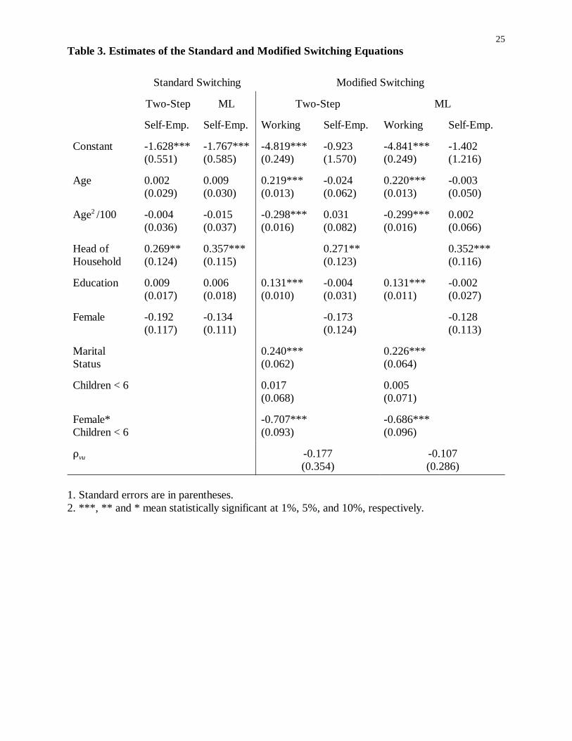
restrictions as can be seen in Table 3. The first two columns of Table 3 present the estimates from
the standard switching regression model. Columns 3-6 of the table contain estimates from the
modified switching regression model where both selection into self-employment or wage-earning

13
jobs and selection into working or non-working are taken into account. Both the standard and
modified switching regression models are estimated using both Heckman’s two-step and ML
methods.
Let us examine the coefficient estimates for the choice between self-employment and wage-
earning jobs across our two models (standard and modified switching regression) by comparing
column 1 to column 4 and column 2 to column 6 in Table 3. Generally, the coefficient estimates
using the modified switching regression model are somewhat different from those using the standard
switching regression model; however, the significance of the estimates, except for the constant term,
has not changed.
We find that the probability of entering self-employment is not significantly affected by age.
Though they are not significant, it is interesting to see that the sign are not as expected in the
modified switching regression model. One possible explanation for the insignificance of the age
variable is that younger individuals are expected to be more receptive to risk. However, in the
context of a transition economy where the financial system is not well developed, these individuals
would have fewer resources to start their own businesses. On the other hand, older individuals may
have accumulated the necessary resources to start their own businesses but are less willing to take
risks. The closer an individual is to retirement, the lower is the probability that he or she would risk
his/her savings. While the variable’s insignificance is troubling, it is not without precedence; using
longitudinal U.S. data, Evans and Leighton (1990) finds that the probability of starting a business
is independent of age.
Head of household is statistically significant and the coefficient estimates are qualitatively
similar across models. The results indicate that the probability of self-employment is greater for
individuals who are heads of households. This may be indicative of the lack of financial constraints

14
amongst heads of households and the predominance of this effect compared with the effect of risk
aversion.
We do not find evidence that education is a significant determinant of self-employment. In
contrast, Earle and Sakova (1999), Gill (1988), and Evans and Leighton (1989), among others, find
that schooling has a substantive positive impact on self-employment choice. However, Fairlie and
Meyer (1996) found no effect. Le (1999) shows that schooling does not always show up to be a
statistically significant determinant of self-employment. Though some earlier papers find that men
choose self-employment more often than women, we do not find that gender is significant in
Hungary.
Columns 3 and 5 show the results for the working or not choice equation for the modified
switching regression model, which is ignored in the standard switching regression model. All the
coefficient estimates, except for children less than six years old, are statistically significant at the
1% level of significance. The coefficient estimates for age suggest that the probability of work
increases up to a certain age and then starts to decline. Investments are made in formal education
with the expectation of increasing one’s earnings, and we find the probability of work increases with
the level of education. The probability of working is significantly higher for married individuals
and the number of children less than six years old significantly decreases a woman’s working status
(female*children < 6).
The correlation coefficient between the residuals in the working equation and the self-
employment equation, Dvu, is insignificant. This implies that the unobserved characteristics which
affect the choice between working and not working do not significantly affect the choice between
self-employment and wage-earning jobs. We turn to the determinants of earnings in the next sub-
section.

15
IV. B. Determinants of Earnings
Various personal and human capital characteristics influence earnings of both the self-
employed and wage earners. Whether an individual lives in Budapest or not is included to control
for the premium of living in the capital. Education and experience (and its square term) are used as
proxies for human capital. Education is expected to have a positive effect on earnings; while the
effect of experience is assumed to initially rise and then fall. Finally, we also control for gender
earnings differentials.
Tables 4 and 5 present the coefficient estimates from the earnings equations for wage-
earners and the self-employed, respectively. Column 1 in both tables presents the OLS estimates.
Estimates of earnings equations based on the standard switching regression model are reported in
columns 2 and 3. Heckman’s two-step and ML methods are used, respectively. Columns 4 and 5
contain estimates of the earnings equations for the modified switching regression model when
Heckman’s two-step and ML methods are used, respectively. For wage earners, the coefficient
estimates of the earnings equation are quite robust across the three models (OLS, standard and
modified switching regression models) and estimation methods (Heckman’s two-step and ML) used.
For example, we find that each additional year of education increases earnings by about 8% using
OLS (column 1). This is reasonably close to the 7.5% we find using the standard switching
regression model estimated using Heckman’s two-step method (column 2) and to the 7.8% we find
using the modified switching regression model (column 4). Similar comparisons can be made for
columns 1, 3 and 5 when the ML method is used. The estimates for the self-employed earnings
equation vary across the models when ML estimation is used. In particular when the work or non-
work choice is taken into account (i.e., in the modified switching regression model), the estimates
of the education and experience parameters are not only larger in magnitude (compared to those in

16
18Using U.K. data, Rees and Shah (1986) also find that the selection bias correction factor isstatistically significant for the regression pertaining to employees but not for the regressionpertaining to the self-employed. As we point out below, this may be because selection intowork/non-work is ignored.
the standard switching regression model) but are now statistically significant at the 5% level.
Before turning to a detailed examination of the influence of observed characteristics on
earnings, we first comment on the sign and significance of the two selection bias correction factors
( and ) included in Heckman’s two-step method to account for the effect of unmeasured
characteristics on the earnings equation (see column 4 of Tables 4 and 5). The negative and
statistically significant estimate for in Table 4 indicates that, given the measured characteristics,
the earnings of individuals who have larger unobserved characteristics, making them more suitable
for wage-earnings jobs, usually earn more in the wage-earnings jobs (i.e., they do better because of
their choice into wage-earning jobs). Note that the choice of wage-earnings jobs in equation (2) is
coded zero. On the other hand, the selection bias correction factor for the choice of self-employment
is not statistically significant in the self-employment earnings equation (see column 4, Table 5).18
This suggests that unobserved characteristics which lead individuals to choose self-employment do
not necessarily increase or decrease earnings. Since our estimate of is not statistically significant
at conventional levels in both earnings equations, there does not appear to be significant selection
bias due to the decision to work or not work.
Measures similar to the λ’s are available in ML. These are the correlation coefficients
between the residuals in the earnings equation and the self-employment equation (Dev) and the
working equation (ρeu). Column 5 of Tables 4 and 5 suggests the importance of accounting for both
types of selection as evidenced by the significant correlation coefficients. For example, in Table 4,
Dev is negative and statistically significant at the 1% level of significance. This result is consistent

17
19This percentage is calculated using exp[ß-.5 V(ß)] - 1, where ß is the estimated coefficient andV(ß) is the variance of ß (see Kennedy, 1981).
with the result for λA as discussed above. In Table 5, ρeu is positive and statistically significant. This
is different from the results using Heckman’s two-step method since the comparable estimate for
λB is not significant. This suggests that unobserved characteristics in the earnings and working
equations for the self-employed are positively correlated, indicative of a positive selection bias. The
observed positive selection bias and the fact that some of the coefficient estimates in columns 3 and
5 in Table 5 are different in magnitude and significance may attest to the importance of accounting
for the work or non-work decision.
In comparing the estimates for the wage earners and the self-employed, we focus on the
results in columns 4 and 5, in particular, column 5 where we use ML. There is a significant earnings
premium for living in Budapest for wage earners but not for the self-employed. Wage earners in
Budapest earn a premium of about 17%.19 Educational attainment is statistically significant in the earnings
equations for both the wage earners and the self-employed at the 10% and 5% levels, respectively. Each additional year
of education increases earnings by about 8% for the wage earners and 9% for the self-employed. Experience has a
positive, and the experience-squared term has a negative effect on earnings. Interestingly, log-earnings for the wage
earners peak at 30 years of experience while for the self-employed, it peaks at 19 years of experience. Not only do the
self-employed on average have higher earnings (see Table 2), they also reach their highest earnings level earlier. This
is because individuals earning wages need to move up the ranks. Finally, gender contributes to earnings differential only
for the wage earners. Female wage earners earn about 23% less than male wage earners.
Lastly, we test whether the returns to all the observed attributes are the same for the wage
earners and the self-employed using a likelihood ratio (LR) test. That is, we test whether there is
a structural difference in the earnings of the wage earners and the self-employed. The null
hypothesis is $0 = $1, where $0 and $1 pertain to the parameters of earnings equation for the wage
earners and the self-employed, respectively. We cannot reject the null hypothesis of the LR test at

18
20The same conclusion is also found with OLS estimates when a similar LR test is applied. 21If the null hypothesis that coefficients of two equations are the same cannot be rejected in a Chowtest, we may estimate the coefficients of “one” earnings equation with pooled sample. However,it should be noted that the finding that the coefficients of earnings equations of self-employed andwage earning jobs are not significantly different does not necessarily imply that earnings in the twosectors can be estimated using the only one earnings equation, since the Chow test assumes that thevariance of two earnings equations should be the same (homoskedasticity). We can easily show thatearnings in the two sectors have different dispersion of stochastic components (i.e.,heteroskedasticity) by implementing another LR test whose null hypothesis is F0 = F1 in addition to$0 = $1. In other words, we are testing whether the return to human capital is the same ($0 = $1) andwhether the dispersion of earnings is the same (F0 = F1). From the results of the LR test, we rejectthe null hypothesis, because the test-statistics are 64.658 for the single switching model and 57.337for the switching and selection model, and are larger than the critical P2 (0.05) value of 14.067 with7 degrees of freedom.
5% level of significance. The calculated P2 statistics are 5.523 and 6.927 for the standard switching
regression and the modified switching regression models, respectively. These values are smaller
than the critical P2(0.05) value of 12.592 at 6 degrees of freedom. The results indicate that overall
returns to measured characteristics are not significantly different for wage earners and the self-
employed.20 This may imply that, in Hungary, returns to observed attributes of the wage earners and
the self-employed do not play a large role in job choice
Our result that overall returns to observed characteristics is not significantly different for
wage earners and the self-employed are consistent with earlier studies using U.K. data (e.g., Rees
and Shah, 1986) and employment data from transition economies (e.g., Earle and Sakova, 2000).
The confidence interval estimates for most of the coefficient parameters for the employee and self-
employed regressions in Rees and Shah (1986) and Earle and Sakova (2000) overlap the
coefficient estimates from the employees’ regression are not significantly different from the
coefficient estimates from the self-employed regression. This suggests those human capital
variables (such as education and experience), and time-invariant person characteristics (such as
gender and race) do not have significantly different impacts on wage earners and the self-employed
in both market and transition economies.21

19
V. Conclusion
This paper estimates earnings functions for the self-employed and for wage-earners in
Hungary in the year 1994. As in other Eastern European countries, Hungary experienced a large
decrease in the employment rate, which cannot be ignored when studying earnings in wage/salary
jobs and self-employment in Hungary in the mid-1990's. The main innovation of the paper is the
introduction of an econometric method for studying a three-state model, including nonemployment
as well as self-employed and wage-earning as separate states. We contrast this “modified
switching” approach with the “standard switching” approach used in most of the literature.
This paper studies earnings determination of self-employment and wage-earning jobs in
Hungary during transition. It is well recognized that the self-employed may have preferences that
differ from those holding wage-earning jobs. The choice of self-employment has been attributed
to people’s attitude toward risk, managerial skills across individuals, financial constraints, and
family background, among other reasons. The role of self-employment in transition has been very
important as documented in various papers. During the transition, many jobs have disappeared due
to, for example, closure of formerly state-owned firms. Self-employment generates jobs when
economies undergo transition from socialist to more market orientation. Hence, examining the
determinants of earnings in both self-employment and wage-earning jobs in economies of transition
is important for understanding the labor market in the transition economies.
Earlier papers have corrected for the bias caused by the choice between self-employment and
wage-earning jobs using the standard switching regression model. This standard switching
regression model has also been applied to studies of earnings determination in labor markets in
transition economies. The novelty of this paper lies in the econometric methodology for estimating

20
earnings equations accounting for two choice problems: first, the potential bias due to the choice
between working and not working and, second, the choice between self-employed and wage-earning
jobs conditional on the choice of working. We have developed the econometrics of the modified
switching regression model which corrects for bias due to both choices. The modified switching
regression model has been estimated using both Heckman’s two-step and maximum likelihood
methods.
Our approach helps improve understanding of the determinants of self-employment/wage
earnings in Hungary. Accounting for the choice between working or not in addition to the choice
between self-employment and wage earning affects the estimates of the earnings equations,
especially for the self-employed. Moreover, according to our hypothesis tests, the earnings
determinants of the two sectors are not significantly different from one another. This may imply that
it is not an earnings premium, but rather non-pecuniary benefits/different preferences toward the two
sectors which determines the choice between self-employment and wage-earning jobs. Finally, we
find evidence of positive selection-bias in the observed earnings for wage earners but find no
selection bias for the self-employed. Workers who chose wage-earning jobs have especially
benefitted from their choice since the unobserved characteristics which led them to choose wage-
earning jobs significantly increase their earnings. However, this is not true for the self-employed;
unobserved characteristics have no impact on earnings.

21
References
Blanchflower, David and Andrew Oswald, “What Makes an Entrepreneur?,” Journal of LaborEconomics 16 (1998): 26-60.
Blank, Rebecca M., “Are Part-Time Jobs Bad Jobs?,” in Gary Burtless, (ed.), A Future of LousyJobs?, (Washington, D.C.: Brookings Institution, 1990).
Blau, David M., “Self-Employment and Self-Selection in Developing Country Labor Markets,”Southern Economic Journal 53 (1985): 351-363.
Blau, David M., “Self-Employment, Earnings and Mobility in Peninsular Malaysia,” WorldDevelopment 14 (1986): 839-52.
Boeri, Tito, Michael C. Burda, and János Köllö, Mediating the Transition: Labour Markets inCentral and Eastern Europe, (London: Institute for EastWest Studies, 1998).
Co, Catherine Y., Ira N. Gang, and Myeong-Su Yun, “Returns to Returning,” Journal of PopulationEconomics 13 (2000): 57-80.
de Wit, Gerrit, “Models of Self-Employment in a Competitive Market,” Journal of EconomicSurveys 7 (1993): 367-397.
Earle, John S. and Zuzana Sakova, “Business Start-Ups or Disguised Unemployment? Evidenceon the Character of Self-Employment from Transition Economics,” Labour Economics 7 (2000):575-601.
Earle, John S. and Zuzana Sakova, “Entrepreurship from Scratch: Lessons on the Entry Decisioninto Self-Employment from Transition Economies,” SITE, Stockholm School of Economics, 1999,http://www.hhs.se/site.
Evans, David and Linda Leighton, “Some Empirical Aspects of Entrepreneurship,” in Zoltan Acsand David Audretsch (eds.), The Economics of Small Firms: A European Challenge (Dordrecht:Kluwer, 1990).
Evans, David and Boyan, Jovanovic, “An Estimated Model of Entrepreneurial Choice underLiquidity Constraints,” Journal of Political Economy 97 (1989): 808-827.
Evans, David, “ The Determinants of Changes in U.S. Employment,” Small Business Economics1 (1989): 111-120.
Fairlie, Robert W. and Bruce D. Meyer, “Ethnic and Racial Self-Employment Differences andPossible Explanations,” Journal of Human Resources 31 (1996): 757-793.
Fishe, Raymond P.H., Robert P. Trost, and Philip M. Lurie, “Labor Force Earnings and CollegeChoice of Young Women: An Examination of Selectivity Bias and Comparative Advantage,”

22Economics of Education Review 1 (1981): 169-191.
Gill, Andrew M., “Choice of Employment Status and the Wages of Employees and the Self-Employed: Some Further Evidence,” Journal of Applied Econometrics 3 (1988): 229-34.
Ham, John C., “Estimation of a Labour Supply Model with Censoring Due to Unemployment andUnderemployment,” Review of Economic Studies 49 (1982): 335-354.
Hamilton, Barton H., “Does Entrepreneurship Pay? An Empirical Analysis of the Returns to Self-Employment,” Journal of Political Economy 108 (2000): 604-631.
Heckman, James, “Sample Selection Bias as a Specification Error,” Econometrica 47 (1979): 153-161.
Johnson, William R., “A Theory of Job Shopping,” Quarterly Journal of Economics 92 (1978): 261-278.
Kennedy, Peter E., “Estimation with Correctly Interpreted Dummy Variables in SemilogarithmicEquations,” American Economic Review 71 (1981): 802.
Kihlstrom, Richard and Jean-Jacques Laffont, “A General Equilibrium Entrepreneurial Theory ofFirm Foundation Based on Risk Aversion,” Journal of Political Economy 87 (1979): 719-748.
Le, Anh T. “Empirical Studies of Self-Employment,” Journal of Economic Surveys 13 (1999): 381-416.
Miller, Robert A., “Job Matching and Occupational Choice,” Journal of Political Economy 92(1984): 1086-1120.
O’Leary, Christopher J., “Promoting Self Employment Among the Unemployed in Hungaryand Poland,” UpJohn Institute Staff Working Paper 99-055, 1999,http://www.upjohninst.org/publications/wp/9955wp.html
Rees, Hedley and Anup Shah, “An Empirical Analysis of Self-Employment in the U.K.,” Journalof Applied Econometrics 1 (1986): 95-108.
Sik, Endre, “Measuring the Unregistered Economy in Post Communist Transition,” EurosocialReport 52 (1995), Vienna, Austria.
Sumner, Daniel A., “Wage Functions and Occupational Selection in a Rural Less DevelopedCountry Setting,” Review of Economics and Statistics 63 (1981): 513-19.
Tunali, Insan, “A General Structure for Models of Double-Selection and an Application to a JointMigration/Earnings Process with Remigration,” Research in Labor Economics 8(B) (1986):235-283.
Vijverberg, Wim P. M., “Consistent Estimates of the Wage Equation when Individuals Chooseamong Income-Earning Activities,” Southern Economic Journal 52 (1986): 1028-1042.
Yuengert, Andrew M., “Testing Hypotheses of Immigrant Self-Employment,” Journal of HumanResources 30 (1995): 194-204.

23Table 1: Labor Market Characteristics for Selected Transition and G7 Counties
Labor ForceParticipationRate (%)1, 2
UnemploymentRate (%)3
Non-WorkingPopulation (%)4
Self-EmploymentRate (%) 5
Self-EmploymentRate (%) 6
1995 1995 1995 1993 1997/1998
Bulgaria 66.7 11.1 40.7 7.6 13.2
Czech Republic 85.7 3.5 17.3 10.4 10.7
Hungary 71.4 10.2 34.8 9.5 13.9
Poland 73.1 15.2 38 20 30.2
Russia 77.8 8.3 28.7 3.5 8.5
Slovak Republic 75 13.2 34.9 7.4 na
France 68.4 11.6 39.5 12 9.1
Germany 71.4 10.4 36 8.5 10.1, 6.1 7
Italy 64.1 12 43.6 na 30.4
U.K. 76.3 8.3 30 12.7 15.6
U.S. 77.3 5.6 27 8.2 14
Sources of data: 1 Total labor force divided by population aged 15-64. 2 From the World Bank’s1997 World Development Report. 3 From the IMF’s International Financial Statistics Database. 4 Includes those not in the labor force and the unemployed. 5 Statistics of Bulgaria, Czech Republic,Hungary, Poland, Russia and Slovak Republic are from Le (1999), Table 1, and the rest are fromEarle and Sakova (2000), Table 1. 6 From Blanchflower et al (2001), see their Table 1. 7 West andEast Germany, respectively.

24Table 2. Mean Characteristics of the Sample 18-65 years old
Working
Both Sexes Everyone Not Working Wage Earners Self-Employed
Sample Size 3145 1544 1480 121
Age (Years) 40.292 42.91 37.72 38.339
Experience (Years) 19.376 19.992
Head of household (Head = 1) 0.435 0.352 0.501 0.686***
Education (Years) 10.159 9.244 11.034 11.14
Female (Women = 1) 0.524 0.552 0.509 0.339***
Marital Status (Married = 1) 0.65 0.597 0.7 0.702
Number of Children under age 6 0.248 0.262 0.239 0.198
Budapest (Living in Budapest = 1) 0.158 0.134 0.18 0.19
Monthly Earnings in Forints 17089.318 22441.694**
Working 0.509
Working
Men Everyone Not Working Wage Earners Self-Employed
Sample Size 1498 692 726 80
Age (Years) 39.505 41.449 37.66 39.438
Experience (Years) 19.609 21
Head of household (Head = 1) 0.696 0.571 0.795 0.888**
Education (Years) 10.201 9.331 10.935 11.063Marital Status (Married = 1) 0.654 0.564 0.731 0.738
Number of Children under age 6 0.254 0.189 0.32 0.225
Budapest (Living in Budapest = 1) 0.156 0.142 0.164 0.2
Monthly Earnings in Forints 19442.249 25223.038*
Working 0.538Working
Women Everyone Not Working Wage Earners Self-Employed
Sample Size 1647 852 754 41
Age (Years) 41.007 44.096 37.777 36.195
Experience (Years) 19.153 18.024
Head of household (Head = 1) 0.198 0.175 0.219 0.293
Education (Years) 10.121 9.174 11.129 11.293
Marital Status (Married = 1) 0.645 0.624 0.67 0.634
Number of Children under age 6 0.243 0.32 0.16 0.146
Budapest (Living in Budapest = 1) 0.16 0.128 0.196 0.171
Monthly Earnings in Forints 14823.763 17014.683
Working 0.483
The null hypothesis tested is that the mean of wage earners is equal to that of self-employed. ***, ** and * meanstatistically significant at 1%, 5%, and 10%, respectively.
25Table 3. Estimates of the Standard and Modified Switching Equations
Standard Switching Modified Switching
Two-Step ML Two-Step ML
Self-Emp. Self-Emp. Working Self-Emp. Working Self-Emp.
Constant -1.628***(0.551)
-1.767***(0.585)
-4.819***(0.249)
-0.923(1.570)
-4.841***(0.249)
-1.402(1.216)
Age 0.002(0.029)
0.009(0.030)
0.219***(0.013)
-0.024(0.062)
0.220***(0.013)
-0.003(0.050)
Age2 /100 -0.004(0.036)
-0.015(0.037)
-0.298***(0.016)
0.031(0.082)
-0.299***(0.016)
0.002(0.066)
Head ofHousehold
0.269**(0.124)
0.357***(0.115)
0.271**(0.123)
0.352***(0.116)
Education 0.009(0.017)
0.006(0.018)
0.131***(0.010)
-0.004(0.031)
0.131***(0.011)
-0.002(0.027)
Female -0.192(0.117)
-0.134(0.111)
-0.173(0.124)
-0.128(0.113)
MaritalStatus
0.240***(0.062)
0.226***(0.064)
Children < 6 0.017(0.068)
0.005(0.071)
Female*Children < 6
-0.707***(0.093)
-0.686***(0.096)
Dvu -0.177(0.354)
-0.107(0.286)
1. Standard errors are in parentheses.2. ***, ** and * mean statistically significant at 1%, 5%, and 10%, respectively.

26Table 4. Log-Earnings for Wage Earners Using the Standard and Modified SwitchingRegression Models
Standard Switching Modified Switching
OLS Two-Step ML Two-Step ML
Constant 8.608***(0.055)
8.402***(0.145)
8.579***(0.063)
8.341***(0.216)
8.549***(0.132)
Budapest 0.161***(0.027)
0.161***(0.027)
0.159***(0.028)
0.161***(0.027)
0.159***(0.028)
Education 0.080***(0.004)
0.075***(0.008)
0.079***(0.005)
0.078***(0.010)
0.080***(0.007)
Experience 0.021***(0.003)
0.018***(0.006)
0.020***(0.004)
0.020***(0.007)
0.021***(0.005)
Experience2 /100 -0.033***(0.008)
-0.027*(0.014)
-0.032***(0.009)
-0.033**(0.017)
-0.035***(0.013)
Female -0.275***(0.020)
-0.152**(0.073)
-0.257***(0.021)
-0.160**(0.070)
-0.258***(0.022)
-1.488*(0.772)
-1.423*(0.737)
0.039(0.085)
Fe 0.401***(0.017)
0.401***(0.017)
Dev -0.527***(0.116)
-0.529***(0.115)
Deu 0.043(0.161)
Adjusted R2 0.32 0.325 0.324
1. Standard errors are in parentheses.2.***, ** and * mean statistically significant at 1%, 5%, and 10%, respectively.

27Table 5. Log-Earnings for the Self-Employed Using the Standard and Modified SwitchingRegression Models
Standard Switching Modified Switching
OLS Two-Step ML Two-Step ML
Constant 9.019***(0.376)
10.176***(1.422)
9.518***(0.594)
10.065***(1.476)
8.481***(0.889)
Budapest 0.190(0.153)
0.191(0.141)
0.190(0.142)
0.191(0.141)
0.192(0.137)
Education 0.053*(0.029)
0.046(0.036)
0.050(0.034)
0.058(0.047)
0.093**(0.043)
Experience 0.032(0.020)
0.029(0.019)
0.030*(0.018)
0.038(0.030)
0.062**(0.026)
Experience2 /100 -0.083*(0.046)
-0.076(0.046)
-0.078*(0.045)
-0.100(0.074)
-0.163**(0.068)
Female -0.278*(0.124)
-0.100(0.250)
-0.203(0.137)
-0.090(0.251)
-0.240(0.154)
-0.602(0.703)
-0.700(0.715)
0.155(0.372)
Fe 0.665***(0.089)
0.763***(0.161)
Dev -0.392(0.265)
-0.331(0.433)
Deu 0.711***(0.234)
Adjusted R2 0.072 0.069 0.064
LR test for $0 =$1
6.684 5.523 6.929
1. Standard errors are in parentheses.2.***, ** and * mean statistically significant at 1%, 5%, and 10%, respectively.
IZA Discussion Papers No.
Author(s) Title
Area Date
558 T. Bauer G. Epstein I. N. Gang
Enclaves, Language and the Location Choice of Migrants
1 08/02
559 B. R. Chiswick T. J. Hatton
International Migration and the Integration of Labor Markets
2 08/02
560 J. W. Budd J. Konings M. J. Slaughter
Wages and International Rent Sharing in Multinational Firms
2 08/02
561 W. J. Carrington P. R. Mueser K. R. Troske
The Impact of Welfare Reform on Leaver Characteristics, Employment and Recidivism
3 08/02
562 J. T. Addison W. S. Siebert
Changes in Collective Bargaining in the U.K.
3 08/02
563 T. Dunne L. Foster J. Haltiwanger K. R. Troske
Wage and Productivity Dispersion in U.S. Manufacturing: The Role of Computer Investment
5 08/02
564 J. D. Brown J. S. Earle
The Reallocation of Workers and Jobs in Russian Industry: New Evidence on Measures and Determinants
4 09/02
565 H. L. van Kranenburg F. C. Palm G. A. Pfann
Survival in a Concentrating Industry: The Case of Daily Newspapers in the Netherlands
3 09/02
566 R. Hujer M. Caliendo D. Radić
Skill Biased Technological and Organizational Change: Estimating a Mixed Simultaneous Equation Model Using the IAB Establishment Panel
5 09/02
567 H. Lehmann K. Phillips J. Wadsworth
The Incidence and Cost of Job Loss in a Transition Economy: Displaced Workers in Estonia, 1989-1999
4 09/02
568 H. O. Duleep D. J. Dowhan
Revisiting the Family Investment Model with Longitudinal Data: The Earnings Growth of Immigrant and U.S.-Born Women
1 09/02
569 J. Haltiwanger M. Vodopivec
Worker Flows, Job Flows and Firm Wage Policies: An Analysis of Slovenia
4 09/02
570 T. K. Bauer S. Bender
Technological Change, Organizational Change, and Job Turnover
1 09/02
571 O. Ashenfelter M. Greenstone
Using Mandated Speed Limits to Measure the Value of a Statistical Life
5 09/02
572 C. Y. Co I. N. Gang M.-S. Yun
Self-Employment and Wage Earning: Hungary During Transition
4 09/02
An updated list of IZA Discussion Papers is available on the center‘s homepage www.iza.org.