Selling an Opaque Product through an Intermediary:

The Case of Disguising One’s Product*

Scott Fay Department of Marketing University of Florida P.O. Box 117155 Gainesville, FL 32611-7155 Phone: 352-392-0161 Ext. 1249 Fax: 352-846-0457 e-mail: scott.fay@cba.ufl.edu

April 2007

(May 2006)

* The author thanks James R. Brown, Rajiv P. Dant, Ganesh Iyer, Chakravarthi Narasimhan, Jagmohan Raju, Steven Shugan, Jinhong Xie, the seminar participants at the Future of Distribution Channels Research Conference, the Summer Institute in Competitive Strategy, Northwestern University, and the University of Florida, and several anonymous reviewers for helpful suggestions. Remaining errors are my own.

1

Selling an Opaque Product through an Intermediary:

The Case of Disguising One’s Product

Abstract:

This paper models multiple service providers who use an intermediary to sell an opaque

product. An opaque product is a product whose identity is concealed from consumers until after

purchase. I find that an opaque good may allow finer segmentation of a service provider’s

customer base, lead to market expansion, and/or reduce price rivalry. However, if there is little

brand-loyalty in an industry, an opaque good increases the degree of price rivalry and reduces

total industry profit. The paper also discusses issues regarding channel structure and outlines

managerial implications of this research.

Keywords: Opaque Products, Pricing, Channels, Intermediaries, Hotwire, Priceline, E-

Commerce

2

Introduction

What is an Opaque Good?

Consider two service providers, A and B, selling their respective services at the prices PA

and PB, respectively. Now suppose an intermediary has a third offering at a price PI. The

intermediary withholds the identity of this good and instead only informs a consumer that if PI is

paid, she will be the awarded either the service provided by firm A or the service provided by

firm B. This stochastic offering by the intermediary is known as an “opaque” good.

Hotwire and Priceline are two prominent examples in the travel industry of intermediaries

specializing in offering opaque goods. For example, one can reserve a rental car through

traditional channels or one can purchase from hotwire.com and receive a car from Avis, Budget,

or Hertz, where the supplier is not revealed until after purchase. Examples of non-travel opaque

goods include: Priceline’s (now discontinued) offerings of automobile insurance, gasoline,

groceries, home financing, new-car sales, and pre-paid long distance service; in the consignment

businesses, apparel manufacturers concealing their brand name by snipping off the tag; package-

goods manufacturers of national brands serving as the (anonymous) suppliers of private labels.

Although both Hotwire and Priceline offer opaque travel products, they determine

transaction prices differently. On Hotwire, consumers see a posted price. On Priceline,

consumers place non-retractable bids � hence, the “Name-Your-Own-Price” slogan. The model

presented in this paper is consistent with the posted price model employed by Hotwire. Previous

papers (e.g., Hann and Terwiesch 2003; Fay 2004; Terwiesch, Savin, and Hann 2005) have

studied the NYOP format, but none of these papers account for how product opacity affects the

market.

3

Research Questions

The press has actively discussed the opaque channel, especially as exemplified by

Priceline. However, there appears to be a divergence of opinions. Some argue that opaque

products purely augment existing markets because they only sell to extremely price-sensitive

consumers who would not have purchased through traditional channels (Coy and Moore 2000,

Dolan 2001, Leo Mullin in Ross 2001). In fact, both Hotwire and Priceline make this argument

in an effort to induce sellers to participate in their respective systems (Dolan and Moon 2000,

McGarvey 2000). On the other hand, competition from yet another channel may further erode

profit margins. Sviokla (2003) asserts that opaque sites will dramatically reduce the level of

prices sustainable in the traditional channels: “Hotels, car-rental companies, and cruise lines are

losing their pricing authority. In all of these industries, there is a strong incentive to provide last-

minute inventory, which starts a cycle of price degradation that will eventually lead to the kind

of price war that is destroying the airlines.” These conflicting views lead to great ambiguity as to

how an opaque product affects traditional channels and thus how potential suppliers should

regard an intermediary. For instance, Leo Mullin, Chairman and CEO of Delta Airlines, says:

“What Priceline really represented was taking inventory that would not otherwise be sold and placing it in the hands of another supplier... You wonder if you have created a channel of discount sales of your product that could substantially cause your product to ultimately be priced lower.”

Although the topic of opaque goods is interesting to consumers, practitioners, and the

popular press, very little formal modeling of opaque products has appeared in the academic

literature. In a much different context, Fudenberg and Tirole (2000) note in passing that a

monopolist could use a stochastic mechanism that offers a “randomization between A and B” to

appeal to switchers. Several recent papers (Wang, Gal-Or, and Chatterjee 2005; Granados,

Gupta, and Kauffman 2005; Fay and Xie 2007) introduce formal models of an opaque good.

4

However, these papers restrict attention to a monopolist. In contrast, this paper considers the case

of multiple service providers. Modeling competition is important for several reasons. First, it

increases consistency with current practice since most examples of opaque goods involve

multiple providers who share a common intermediary. Second, since Fay and Xie (2007) show

that offering an opaque good is most advantageous when the component goods are not too

vertically-differentiated, a firm that does not produce multiple, horizontally-differentiated goods

may need to utilize an intermediary in order to introduce an opaque product. For example, it may

not make sense for Avis to create its own opaque product using only its own product offerings

(e.g., an Avis compact car or an Avis midsize car). Instead, Avis may want to enlist the services

of Hotwire so that the opaque good is either an Avis compact car or a Budget compact car. Third,

there may be logistical advantages to using an intermediary rather than developing one’s own

opaque product. For example, an intermediary such as Hotwire has invested in developing

awareness for what an opaque product is. New service providers are easily added to this system.

On the other hand, to offer one’s own opaque good, a service provider must educate its

consumers and present the offering in a way that avoids confusion. This is not trivial since it may

require placing additional restrictions on consumers who purchase the opaque good, e.g., a no-

refund / non-transferable policy, which a retailer does not wish to impose on its other non-

opaque services.

Consistent with Peterson and Salasbramanian (2002), this paper views the opaque

channel as a complement to traditional channels. As such, the introduction of competing rival

service providers and an intermediary leads to several interesting research questions:

1. How will the introduction of an opaque product affect the prices of non-opaque goods?

2. How will an opaque good affect industry profitability?

3. How many consumers and what types will be attracted to an opaque product?

5

4. How will answers to the previous questions depend on how many units are allocated to the opaque channel?

5. Under what conditions would a service provider choose to use the opaque channel?

Overview of Key Results

For a monopolist, adding an opaque good cannot reduce profits. Suppose a monopoly

sells two different products in the absence of an opaque good. The firm could replicate this profit

by setting the price of the opaque good high enough that no units of the opaque good are sold.

However, the firm can usually do even better either by: a) introducing an opaque good at a

discount sufficiently large to attract additional consumers but not so large as to cannibalize any

existing sales; or b) introducing an opaque good at little, if any, discount and then raising the

prices of the traditional goods. Thus, an opaque good can enhance profit through either market

expansion or by enhancing price discrimination of one’s existing customer base.

In the focal model of this paper, two service providers use an intermediary to sell the

opaque product. I find that if there is little brand-loyalty in an industry, an opaque product

magnifies price competition and thus reduces industry profits. However, if there is a significant

amount of brand-loyalty in an industry, an opaque good curtails price competition and thus

increases industry profits. Furthermore, the degree of price rivalry depends on how many units

are allocated to the opaque channel. Interestingly, it is possible that industry profit falls if the

opaque channel is given a small allocation but increases if given a large allocation.

Other Related Literature

The literature has considered many forms of price discrimination. If firms can identify

individual consumers or their characteristics, e.g., new versus repeat customer, firms may be able

to customize prices (Chen, Narasimhan, and Zhang 2001; Villas-Boas 1999, 2004). However, in

this paper, I assume firms do not have such private information. Other mechanisms, e.g.,

6

coupons, may facilitate price discrimination via self-selection (Narasimhan 1984). Product lines

can also lead to market segmentation (e.g., Moorthy 1984; Gerstner and Holthausen 1986; Desai

2001). Recent research has explored how the advent of the Internet can increase the ability and

ease of such product differentiation. For example, Varian (2000) shows that manufacturers

(especially those of information goods) can benefit from creating multiple versions of the same

underlying product. An interesting result is that versioning can be profitable even if there is no

cost-advantage from reducing quality (Deneckere and McAfee 1996). An opaque good could be

viewed as an example of a lower-quality version of an existing product. Introducing an opaque

good avoids many of the costs associated with developing a new product because none of the

features of the product (or service) have themselves been altered but, instead, are simply hidden

from consumers. Thus, this new product is relatively simple to introduce (e.g., signing up with a

third-party site such as Hotwire) and technological advances such as enhanced computational

speed make implementation feasible for a growing array of products and services since there are

lower costs to aggregation and arbitrage can be eliminated (Shugan 2004). For example,

technologies such as smart cards, RFID, and electronic tickets, allow for the enforcement of the

no refund / non-transferable restrictions which are necessary for the opaque product to be viable.

Furthermore, in contrast to the previous versioning literature, this paper introduces an

intermediary and multiple service providers. Thus, the model enables exploration of how an

intermediary’s entry affects competition between firms.1

Previous studies have also considered how various types of intermediaries impact a

market (e.g., referral infomediaries, Chen et al. 2002; mass customization, Chen and Iyer 2002).

This current paper extends the literature to a type of intermediary that has not been previously

considered. Furthermore, this paper joins a large literature that studies competition between

7

channels (e.g., Balasubramanian 1998; Coughlan and Soberman 2005; Zettelmeyer 2000).2 In

these papers, as in this one, the appeal of each channel differs across consumers. However, in

this paper, the product itself differs across channels; in the aforementioned papers, physical

locations (or lack thereof when considering direct retailers) are the source of differentiation

across channels.

The Model

Two service providers, A and B, have unlimited capacity and symmetric costs of

production, which without loss of generality are assumed to be zero. Later, I discuss the impact

of adding capacity constraints to the model. The sequence of the game is given in Figure 1. In the

first stage, the service providers contract with the intermediary, that is, they decide how many

units to allocate to the opaque channel and agree to transfer payments, if any. Both A and B, but

not consumers, observe the outcome of stage I. In stage II, service providers simultaneously

choose their respective prices, PA and PB. Then, having observed PA and PB, the intermediary

chooses the price of the opaque good, PI.3 This sequential pricing framework, consistent with

Wang et al. (2005), is used since a pure-play Internet intermediary may have more flexibility in

pricing than traditional service providers (e.g., due to technological advantages and not being

constrained by the need for consistency across multiple channels: Internet, phone, ticket

counters). Furthermore, since in most observed situations the service providers (e.g., major

airlines and hotel chains) are much larger and well-established than the intermediary (e.g.,

Hotwire), it seems likely that the intermediary responds to service providers’ prices rather than

vice-versa. In the final stage of the game, risk-neutral consumers make purchase decisions to

maximize expected surplus. Consumers do not know the source of the opaque good. They expect

to be assigned to provider A with probability ½ and to provider B with probability ½. Later, I

8

discuss the incentive to keep the source hidden.

Figure 1 Game Setup I. Contracting II. Service providers simultaneously choose prices

III. The intermediary chooses the price of the opaque good IV. Consumers decide which service to purchase, if any

Consumer Demand

I use a generalization of the loyals/switchers model (Narasimhan 1988; Varian 1980;

Chen, Narasimhan, and Zhang 2001).4 There are two types of consumers, brand-loyals and

searchers, each of whom purchases at most one unit. Brand-loyals make up ρ proportion of the

population, which is normalized to one. A brand-loyal consumer does not consider all available

product offerings but instead simply visits her preferred firm and purchases as long as the price

does not exceed her reservation value, which is assumed to equal VH ( )1≥ for all brand-loyals.

The model is silent as to the source of this loyalty. For example, consumers could be loyal

because they are not aware of the other product offerings, have very strong preferences for their

preferred good, are locked-in to a loyalty program (e.g., frequent flier program), or face some

other constraint (e.g., company policy or contract). See Srinivasan, Anderson, and Ponnavolu

(2002) and the literature cited therein for a further discussion of potential sources of firm loyalty.

A key question in this paper is how the magnitude of ρ impacts the pricing equilibrium and the

profitability of the opaque product. To ease tractability and exposition, I assume a symmetric

distribution of the brand-loyals, i.e., half ( )2ρ are loyal to firm A and the other half are loyal to

firm B.

The remaining 1- ρ consumers are searchers. This segment is represented by a Hotelling

model in which consumers are uniformly distributed along a segment of length one. Each

9

searcher’s location (x) represents that consumer’s ideal product. Firms A and B are assumed to

be located at the endpoints of the line segment, at 0 and 1, respectively. The reservation value of

each searcher’s ideal product is normalized to one. Let t be the fit cost loss coefficient from not

receiving one’s ideal product. Thus, a consumer located at x incurs a disutility of t x if she buys

from firm A and a disutility of t (1-x) if she buys from firm B. Each searcher’s expected disutility

for the opaque good equals t/2: (1 )2 2 2tx t x t−+ = .

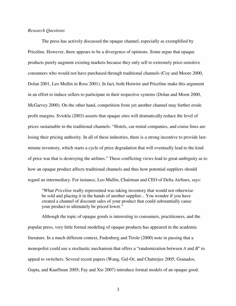
Figure 2 illustrates consumers’ expected net value for each of the three product offerings.

All consumers to the left of x = ½ strictly prefer service A to service B or the opaque good; all

consumers to the right of x = ½ strictly prefer service B to service A or the opaque good. No one

strictly prefers the opaque good. Thus, although services A and B are only horizontally-

differentiated, i.e., are of comparable quality, the intermediary’s opaque product is perceived as

being strictly inferior. This is not due to inferior quality because consumers who purchase the

opaque good are assured of receiving either service A or service B, not some other sub-par

service.5 The opaque good is inferior because there is a positive probability of receiving one’s

less preferred product. Adding risk aversion to the model would further reduce the value of the

opaque product. An obvious outcome of this tiered demand is that the intermediary must price

below the traditional prices if it is to make any sales.

10

Figure 2 Net Utility of Searchers 1 VA = 1- t x VB = 1- t (1-x) Net Utility

VI = 1- t/2 1-t 0 ½ 1 x

This model allows for several dimensions of heterogeneity in demand. First, the division

between brand-loyals and searchers captures the fact that firms may serve segments of users

with different reservation values and very different degrees of price-sensitivity. Second, in

contrast to the loyals/switchers models used in the previous literature, this model allows for

heterogeneity within the price-sensitive segment, which is why these consumers are labeled

“searchers” rather than “switchers”. This allows for heterogeneity of tastes even among the

segment of consumers that are open to purchasing either good “if the price is right.”

When interpreting the model, ρ provides a measure of brand-loyalty within an industry

(which may be a function of product differentiation but could also be influenced by other factors

such as the prevalence of loyalty programs). The parameter t represents the strength of consumer

tastes among those price-sensitive consumers and thus varies across product categories

depending on the degree and importance of product differentiation. For example, the t in the

market for hotel rooms is higher than the t in the market for rental cars since hotels naturally vary

in locations and amenities offered whereas rental car companies offer rather homogenous

services.6 For the remainder of the paper, I assume the following two conditions hold:

11

ρρ

−−<

3)1(2

t (1)

( )1 Ht Vρ ρ> − (2)

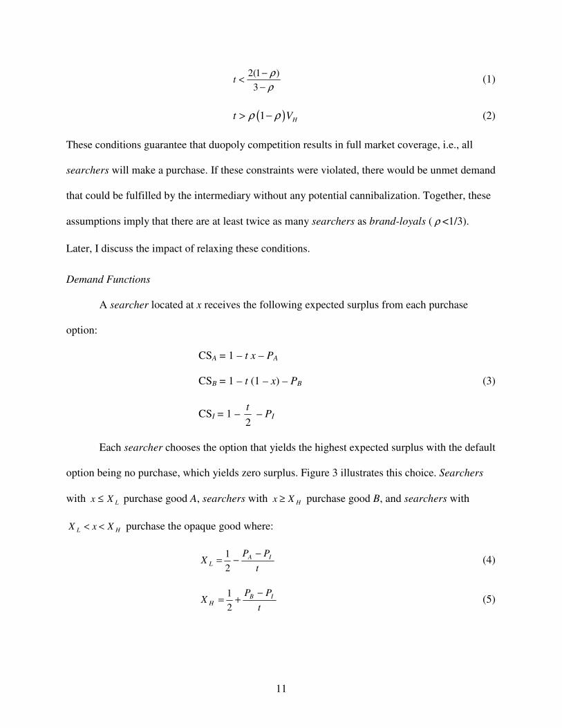
These conditions guarantee that duopoly competition results in full market coverage, i.e., all

searchers will make a purchase. If these constraints were violated, there would be unmet demand

that could be fulfilled by the intermediary without any potential cannibalization. Together, these

assumptions imply that there are at least twice as many searchers as brand-loyals ( ρ <1/3).

Later, I discuss the impact of relaxing these conditions.

Demand Functions

A searcher located at x receives the following expected surplus from each purchase

option:

CSA = 1 – t x – PA

CSB = 1 – t (1 – x) – PB (3)

CSI = 1 – 2t

– PI

Each searcher chooses the option that yields the highest expected surplus with the default

option being no purchase, which yields zero surplus. Figure 3 illustrates this choice. Searchers

with LXx ≤ purchase good A, searchers with HXx ≥ purchase good B, and searchers with

HL XxX << purchase the opaque good where:

t

PPX IA

L−

−=21 (4)

t

PPX IB

H−

+=21 (5)

12

Figure 3 Searchers’ Optimal Purchase CS 1-PA CSA CSB

CSI 0 XL XH 1 x

Monopoly

As a baseline case, consider a single firm that owns both brand A and brand B. Such a

monopolist could offer its own opaque good and thus capture the entire profit available for the

three product offerings.7 Proposition 1 states the unambiguous benefit from the opaque good.

Proposition 1: A monopolist strictly improves its profits by offering an opaque product. The additional profit from adding the opaque good to the firm’s product line is at least

( )( )122

−+ HVtρ .

If the monopolist does not offer an opaque good, its optimal prices are2

1t

PP BA −== ,

which results in complete market coverage. The profit to the monopolist is:

2

1tNI

M −=Π (6)

Condition (1) guarantees that full coverage of the searcher market is more profitable than only

partial coverage of this segment. Condition (2) ensures that it is not profitable to deviate to the

prices of HBA VPP == and thus only sell to brand-loyals.

Now suppose the monopolist also offers an opaque good. Notice that as PI falls, the

surplus from purchasing the opaque good rises and sales are shifted to the lower-margin opaque

13

good. To minimize this cannibalization effect, a monopolist chooses PI=1-t/2. This ensures that

all consumers will purchase something (as long as HA VP ≤ and HB VP ≤ and thus brand-loyals

also purchase). By choosing HBA VPP == , the monopolist would sell the opaque good to all

searchers and sell traditional goods to the brand-loyals. These prices result in a profit of:

( ) ��

���

� −−+=Π2

11t

VHM ρρ (7)

The profit from (7) is strictly higher than (6) with the magnitude of this difference given in

Proposition 1. Under some situations, the monopolist can earn profits in excess of (7) by selling

traditional goods to some searchers, thus increasing the magnitude of the advantage of offering

an opaque good above what is stated in Proposition 1. Details are provided in the appendix.

Competition

Opacity of the Intermediary’s Product

So far, I have assumed the intermediary’s product is opaque, i.e., consumers do not know

if they will get service A or service B if they purchase from the intermediary. Suppose that in

stage I, contracting with the intermediary results in QA (QB) units of service A (B) being made

available to the intermediary. Obviously, these allotments and the marginal transfer price of each

service affect the “true” probability that the opaque good will originate from a particular service

provider. The model assumes consumers cannot observe this “true” probability and instead

believe that each service is equally likely to be awarded. This subsection explores when such an

assumption is plausible.

To begin the discussion, assume consumers cannot observe allocations by the service

providers to the intermediary. This seems plausible. Contracts between businesses are

proprietary information. In practice, neither customers nor researchers observe which supplier

14

has made units of its inventory available to Hotwire.8 Although allocations are not observable,

one might wonder whether the intermediary or the service providers have an incentive to

voluntarily disclose this information. There are several reasons to believe voluntary disclosure

will not occur. First, contracts may contain non-disclosure clauses. In many various situations,

we know contracts include such clauses and often with severe penalties for violations. Second,

even in the absence of enforceable non-disclosure clauses, signaling is unlikely to be desirable or

credible. Consider the intermediary. Its business model is predicated on selling an opaque good.

Even if there were a short-term gain from signaling a product’s identity, such disclosure would

tarnish the intermediary’s reputation and thus eliminate or significantly curtail its ability to make

future sales (in this and other product categories). Now turn to the service providers. A service

provider who signaled an opaque product’s identity would hurt its relationship with the

intermediary. Furthermore, even if the short-run advantage from signaling were sufficiently

large, signals are unlikely to be credible. Specifically, provider A may gain from having

consumers believe the opaque good comes from provider B (so that some consumers switch from

the opaque good to good A). But, the same argument applies to provider B. If each firm tries to

signal the opaque good comes from its rival, the message is mixed and consumers remain

uninformed as to the source of the opaque product.

As a result of this opacity, when deriving the pricing equilibrium, one only needs to

consider the total number of units available to the intermediary ( )BATOT QQQ += , not the

proportion that comes from each particular service provider.

Pricing: No Intermediary

In the absence of an intermediary (i.e., QTOT = 0), define X̂ as the searcher who is

indifferent between purchasing service A at PA and purchasing service B at PB:

15

t

PPX AB −

+=21ˆ (8)

Firm A’s profit is: ( ) ˆ12A AP XρΠ ρ� �= + −� �

� �. Firm A’s best response to PB is: ( ) ( )

( )1

2 1B

A B

P tP P

ρρ

− +=

−.

Firm B’s best response is symmetric to A’s. Thus, the equilibrium prices are:

ρ−

==1

tPP NI

BNI

A (9)

Condition (1) guarantees a searcher located at x= ½ is willing to purchase in equilibrium. Thus,

there is complete market coverage and profit is:

( )ρ−=Π=Π

12tNI

BNIA (10)

Condition (2) guarantees each firm prefers this outcome to selling only to one’s brand-loyals (at

a price of VH and a profit of 2

HVρ ).

Pricing: Active Intermediary

Now turn to the case where the intermediary is active in the market, i.e., QTOT > 0. In this

section, I consider how prices depend on the level of QTOT. Then, in the subsequent sections, I

calculate the associated profits and then derive the optimum contracts which will determine what

QTOT will be the equilibrium for the full game.

QTOT and ρ control how aggressively the intermediary and service providers compete on

prices. These parameters determine which of six different pricing outcomes occur. The appendix

contains the derivation of equilibrium prices, with Table A1 reporting the six possible pure

strategy equilibria. These equilibria differ according to whether the intermediary faces a binding

constraint when choosing its price and whether both, only one, or neither service provider

concedes the searcher market in order to focus on their brand-loyals (i.e., Pi = VH). Throughout

16

the analysis, I assume the intermediary does not pay per-unit fees to the service providers. This

assumption will be justified later when contracts are discussed. Furthermore, transfer payments

by the intermediary to the service providers are ignored since these are sunk costs at the time

pricing decision are made.

Proposition 2 summarizes the impact of an opaque intermediary on prices and revenue

from traditional sales:

Proposition 2: If an opaque intermediary has a positive market share, each service provider generates less revenue from sales of its traditional service.

The impact of an opaque intermediary on prices is:

1. If the number of units allocated to the opaque channel is sufficiently small or if there is sufficiently little brand-loyalty in an industry, entry by an opaque intermediary reduces the prices of traditional services.

2. If the number of units allocated to the opaque channel is sufficiently large and there is sufficient brand-loyalty in an industry,

a. Entry by an opaque intermediary increases the prices of traditional services. b. The price of the opaque good is higher than the prices of traditional services

in the absence of the intermediary.

The key result from Proposition 2 is that entry by an opaque intermediary may lead to

reduced price competition. For example, in the “concession” equilibrium, both service providers

find it more profitable to sell exclusively to their brand-loyals (at A B HP P V= = ) rather than

compete for the searchers with the intermediary. Notice that the intermediary might be

particularly aggressive since it does not have any brand-loyal segment of its own and thus must

rely on a price advantage in order to attract customers. Furthermore, in the concession

equilibrium, facing service providers with prices A B HP P V= = , the intermediary maximizes its

profit by selling the opaque product to all searchers at a price of 12I

tP = − . Notice that relative to

the no intermediary case, in this concession equilibrium brand-loyals end up paying a higher

price for the same service. Searchers also pay higher prices (and now get an opaque product

17

which may end up being their less-preferred service).

However, this effect of relaxing competition (as occurs in the concession equilibrium),

will only occur under certain conditions. In particular, as the amount of inventory the

intermediary has at its disposal decreases (i.e., QTOT falls), the intermediary will be less

aggressive if a service provider were to attempt to sell to searchers since the intermediary only

has the ability to serve a smaller number of searchers. Recognizing this, if QTOT is sufficiently

small, either one or both service providers would earn more profit by selling to some searchers

rather than selling exclusively to its brand-loyals. Furthermore, conceding all the searchers will

not be the most profitable alternative for a service provider if there are few brand-loyals ( ρ is

relatively small). Thus, if either QTOT or ρ is sufficiently small, at least one of the service

providers will compete for the searchers with the intermediary. For example, in the “strong

competition” equilibria, all three firms sell to searchers as illustrated in Figure 3.

Entry by the intermediary causes prices to fall since each service provider competes for

searchers against an additional product. The intermediary has to discount its prices even further

to capture any market share.

Finally, Proposition 2 shows that, regardless of which equilibria results, an active

intermediary reduces the revenue from traditional sales. For example, under “strong

competition” service providers both get lower prices per unit sold and make fewer traditional

sales. Under “concession,” each service provider earns higher revenue per sale but makes

drastically fewer sales.

Profitability

The previous section indicates sales of the opaque good come at the expense of

traditional sales. However, the intermediary must induce service providers to participate in order

18

to enter the market. Sufficient compensation is feasible (i.e., large enough to induce participation

by the service provider, but small enough to be on net profitable for the intermediary) only if the

combined profit of the intermediary and one service provider exceeds the profit a service

provider earns in the absence of the opaque good:

[ ] NIA I AE Π Π Π+ > (11)

Lemma 1 summarizes when condition (11) is met:

Lemma 1: Condition (11) is satisfied only if

(a) In equilibrium, both firms concede the searcher market and a sufficient number of units are allocated by the service providers to be sold as the opaque good; or

(b) In equilibrium, only one firm concedes the searcher market and the number of units allocated by the service providers is not too large and not too small.

Corollary 1: Condition (11) cannot be satisfied if neither firm concedes the searcher market in equilibrium.

The appendix provides the details supporting Lemma 1 and Corollary 1. Notice that the

market is fully covered in the absence of the intermediary. Thus, for any symmetric equilibrium,

condition (11) can be satisfied only if the average selling price increases with entry. If all firms

compete for the searchers, e.g., “strong competition”, the price paid by each consumer falls and

thus condition (11) cannot be met. On the other hand, under “concession” each consumer ends

up paying a higher price in equilibrium, thus ensuring condition (11) is satisfied. Finally, if only

one firm concedes the searcher market, there will still be competition for searchers between the

intermediary and the other firm. If QTOT is too small, the traditional firm that remains in the

searcher market sets a very low price in order to capture the searchers who cannot be served by

the intermediary. On the other hand, if QTOT is too large, competition between the intermediary

and the remaining traditional firm will be fierce. Thus, when a single firm concedes, condition

(11) is satisfied only for intermediate values of QTOT.

19

Joint-Profit Maximization

The service providers, through the choice of QTOT, can influence which equilibria will

occur (and the level of prices and profit in the constrained equilibria). In this section, I present

the QTOT that maximizes the LHS of (11), noting that one can reach NIAΠ with QTOT =0. Define Q*

as the minimum QTOT such that:

( ) ( ) ( ) ( )* *A I A TOT I TOTE Q Q E Q QΠ Π Π Π� � � �+ ≥ + 0≥∀ TOTQ (12)

Figure 4 illustrates the value of Q* over the relevant parameter range. The bold lines

represent conditions (1) and (2) which guarantee full coverage in the absence of the

intermediary. In the left-most region (Q*=0) where there is very little brand-loyalty, neither

service provider would concede the searcher market regardless of the size of QTOT. Thus, joint

profit is maximized at QTOT =0 where the competitive threat from the opaque intermediary is the

lowest. In the far-right region ( )ρ−=1*Q where brand-loyalty is rather sizable, both service

providers will concede the searcher market if QTOT is large enough. Thus, joint-profit is

maximized at a level that both induces concession and enables the intermediary to sell to all

searchers. Finally, for intermediate levels of brand-loyalty, it is not possible to get both service

providers to concede the searcher market but one firm would opt out of the searcher market if

QTOT is sufficiently large. Lemma 1 (b) ensures that condition (11) can be satisfied when there is

a single concession. Thus, Q* must be strictly positive in this case.

20

Figure 4 Illustration of Q*

Contracts

From the intermediary’s perspective, services A and B are perfect substitutes. Thus, if the

service providers engage in linear pricing, the intermediary would satisfy its entire demand for

the opaque good using the lower priced firm. As a result, equilibrium wholesale prices cannot

exceed marginal costs. To allow for a richer set of contracts, this paper lets contracts include

lump-sum transfer payments. However, as Shaffer and Zettelmeyer (2002) note on p. 279, when

goods are perfect substitutes, there will be an extremely skewed division of profits. For example,

in the current model, if the service providers make sequential contract offers to the intermediary,

the first-mover receives the entire incremental profit associated with this additional channel.

With such an asymmetric division of profit, one may question whether the results are unduly

dependant upon the game’s bargaining structure. I address this concern by considering a variety

of bargaining structures. Proposition 3 summarizes the results of this analysis:

Q*=0 Q*>0

Q*=1- ρ “concession”

32

t

ρρρρ

( )ρρ

−−<

312

t

( ) HVt ρρ −> 1

0

21

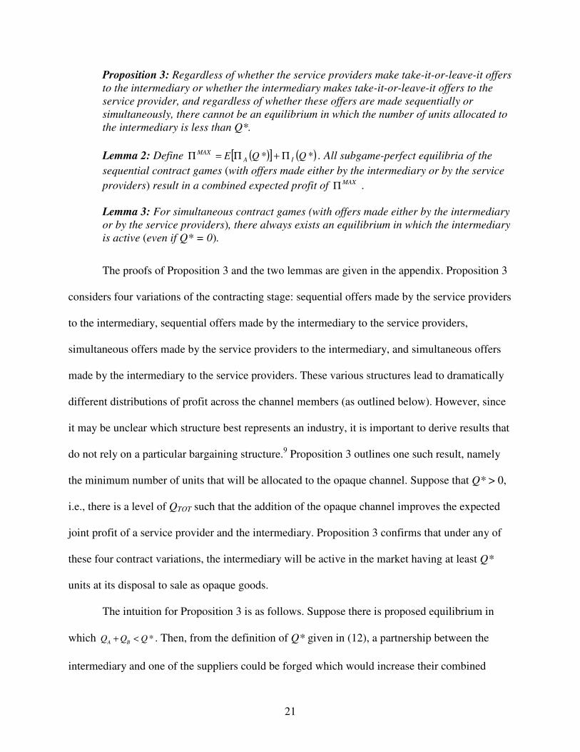
Proposition 3: Regardless of whether the service providers make take-it-or-leave-it offers to the intermediary or whether the intermediary makes take-it-or-leave-it offers to the service provider, and regardless of whether these offers are made sequentially or simultaneously, there cannot be an equilibrium in which the number of units allocated to the intermediary is less than Q*. Lemma 2: Define ( )[ ] ( )** QQE IA

MAX Π+Π=Π . All subgame-perfect equilibria of the sequential contract games (with offers made either by the intermediary or by the service providers) result in a combined expected profit of MAXΠ . Lemma 3: For simultaneous contract games (with offers made either by the intermediary or by the service providers), there always exists an equilibrium in which the intermediary is active (even if Q* = 0).

The proofs of Proposition 3 and the two lemmas are given in the appendix. Proposition 3

considers four variations of the contracting stage: sequential offers made by the service providers

to the intermediary, sequential offers made by the intermediary to the service providers,

simultaneous offers made by the service providers to the intermediary, and simultaneous offers

made by the intermediary to the service providers. These various structures lead to dramatically

different distributions of profit across the channel members (as outlined below). However, since

it may be unclear which structure best represents an industry, it is important to derive results that

do not rely on a particular bargaining structure.9 Proposition 3 outlines one such result, namely

the minimum number of units that will be allocated to the opaque channel. Suppose that Q* > 0,

i.e., there is a level of QTOT such that the addition of the opaque channel improves the expected

joint profit of a service provider and the intermediary. Proposition 3 confirms that under any of

these four contract variations, the intermediary will be active in the market having at least Q*

units at its disposal to sale as opaque goods.

The intuition for Proposition 3 is as follows. Suppose there is proposed equilibrium in

which *A BQ Q Q+ < . Then, from the definition of Q* given in (12), a partnership between the

intermediary and one of the suppliers could be forged which would increase their combined

22

profit by raising the service provider’s allocation by Q* - QA - QB units. Thus, with appropriately

defined transfer fees, it must be possible to increase the profits of each of the partner firms.

Therefore, the original allocation must not have been an equilibrium.

It is also interesting to consider the equilibrium distribution of profits. Not surprisingly, it

turns out that this distribution is heavily dependant on the underlying bargaining structure.

Suppose, in equilibrium, firm A provides QA units to the intermediary for a transfer payment

ofα and firm B provides QB units to the intermediary for a transfer payment of β . Then, firm A

earns a net profit of ( )A A BE Q QΠ α� �+ + , firm B earns a net profit of ( )A A BE Q QΠ β� �+ + , and the

intermediary earns a net profit of ( )I A BQ QΠ α β+ − − . Consider the following scenarios.

Sequential offers by the service providers: Suppose service provider A offers (QA, α ),

this offer is either accepted or rejected by the intermediary, then service provider B offers (QB,

β ), and then this offer is either accepted or rejected by the intermediary. The subgame perfect

equilibrium results in net profit of ( ) ( )* *A IE Q Q� �+ for firm A, a net profit of ( )*AE Q� � for

firm B, and no net profit for the intermediary. Thus, the service provider that moves first is able

to obtain the entire incremental benefit that comes from introducing an opaque good.10

Sequential offers by the intermediary: Suppose the intermediary makes sequential offers,

first to service provider A (offering to pay α for QA units), then to B (offering to pay β for QB

units). The subgame perfect equilibrium results in both firms A and B earning a net profit

of ( )*AE Q� � , and the intermediary earning a net profit of ( )*I QР. This bargaining structure

puts the intermediary in the position of power. The intermediary can effectively play the service

providers off each other. Firm A knows that if it doesn’t accept the intermediary’s offer, its rival

will. Since firm A views entry by the intermediary as inevitable, the intermediary can use its first

contract offer to induce provider A to meet the entire demand, i.e., QA = Q*, with only a token

23

payment (and, in the process, eliminate the need to make any payment to service provider B).

Simultaneous offers: Modeling simultaneous rather than sequential contracts introduces

additional complexities. Multiple equilibria can arise with the variations across equilibria not

only in terms of how profits are allocated among the channel members and in the source of the

opaque units but also in terms of market prices and overall market profitability. Expectations

about a rival’s action play a crucial element in the analysis. Take an extreme example where

Q*=0. With sequential offers, the unique equilibrium is for the intermediary to be inactive.

However, with simultaneous offers (regardless of whether offers are made simultaneously by the

service providers or by the intermediary) other equilibria also exist. Let Q~

be the QTOT that

maximizes ( )TOTI QΠ . There is an equilibrium in which Q~

units are allocated to the intermediary.

This equilibrium is sustained by each firm’s belief that the other will contract with the

intermediary. These beliefs are rational since if firm A believes that firm B will contract with the

intermediary, then firm A would want to too (even with just an epsilon transfer payment from the

intermediary) and vice-versa. In the limit, each service provider earns a net profit of ( )AE Q� �

�

and the intermediary earns a net profit of ( )I QΠ � . The intermediary is able to retain the entire

revenue from opaque good sales without making any substantial transfers to the service

providers. Thus, when Q*=0, we have an equilibrium in which the intermediary has no presence

in the market and another where the intermediary has so many units at its disposal that it reaches

the apex of the possible profit from opaque sales.

For this example, from A and B’s perspective, the active-intermediary equilibrium is

Pareto-inferior since profits for each would strictly be higher if they could coordinate on the

0== BA QQ equilibrium. The literature is divided on the likelihood of experiencing Pareto-

24

inferior equilibria. On one hand, Anderlini (1999) argues that there is “consensus that the Pareto-

inferior equilibrium ... is, in some sense, unlikely to prevail.” Research on the impact of pre-

game cheap talk (Arvan, Cabral, and Santon 1999; Clark, Kay, and Sefton 2000), repeated play

of a static game (with noise) (Lagunoff 2000) and the psychological salience of equilibria to

decision makers (Colman 1997) lends support to this view. However, Anderlini (1999) also

acknowledges that Pareto-inferior equilibria are stable and survive most refinements that have

been put forward in the literature. Furthermore, Cooper and John (1988) provide a literature

review containing many examples in which coordination failures arise. Such failures are

frequently cited as the reason for macroeconomic underperformance (Azariadis 1981, Azariadis

and Drazen 1990, Matsuyama 1991, Baland and Francois 1996). Thus, it seems possible that

simultaneous contracts could result in participation by an opaque intermediary in cases where its

impact unambiguously harms the service providers.

Discussion

The analysis thus far makes several important assumptions. First, I have restricted

attention to situations when there is full coverage of the searcher market even in the absence of

the opaque channel. Second, service providers are not capacity constrained. In this section, I

discuss the impact of relaxing these assumptions and then provide an overview of the results,

giving particular attention to outlining several managerial implications.

First, consider the assumption that there is full coverage in the absence of the opaque

channel, i.e., conditions (1) and (2) are satisfied. If one of these conditions is violated, there is

unmet demand in the absence of an opaque intermediary. Since the firms could allocate some

units to the intermediary without having any impact on its traditional sales, it must be the case

that Q* > 0.11 Furthermore, if fewer searchers are buying in the absence of an opaque good,

25

service providers are more likely to focus on brand-loyals if an opaque intermediary becomes

active. Thus, expanding consideration to parameters beyond the basic model increases the

probability that an opaque intermediary will be active and that entry relaxes price competition.

Now turn to the assumption that service providers are not capacity constrained. Suppose

each service provider has the capacity to produce T units at zero marginal cost. The base model

assumes that either firm could serve the entire searcher market 12

Tρ� �≥ −� �

� �. This assumption can

be relaxed without dramatically affecting results. For example, with weak capacity constraints

11

2 2T

ρ� �≤ < −� �� �

, additional analysis shows that Q* is not dependent on T. However, transfers from

both service providers are needed to reach Q*. Thus, one party cannot extract the entire

incremental value of the opaque channel. Consequently, weak capacity constraints result in less

skewed allocations to the intermediary and in a less skewed distribution of profit.

On the other hand, if capacity constraints are very severe2

Tρ� �<� �

� �, Q* = 0. Each firm

cannot even meet the entire demand from its brand-loyals. Thus, there is no advantage to

reserving any units for the opaque channel.

In between these two extremes 12 2

Tρ� �< <� �

� �, the opaque good is less valuable relative to

the base model. First, the potential number of units available to be sold to searchers falls as

constraints become more severe (T falls). Suppose both service providers will concede the

searcher market. After sales to brand-loyals have been subtracted, 22

Tρ� �−� �

� �total units are left

over. As constraints become more severe, i.e., T approaches 2ρ , the number of units to be

transferred to the intermediary falls. Second, the probability that Q* = 0 increases as constraints

26

become more severe. Suppose that in the absence of the intermediary, each firm would have sold

to some searchers (at a price that exceeds any consumers’ value for the opaque good). As

constraints become more severe, this no-intermediary price increases. Thus, in contrast to

Proposition 2b, when capacity constraints are rather severe, entry by an opaque intermediary

necessarily decreases the revenue earned from each searcher and as constraints become even

more severe service providers face a greater sacrifice per sale transferred to the intermediary.

Summary of Results

To summarize, this paper includes findings involving on four dimensions:

1. Appeal to consumers: An opaque good appeals to consumers with weak preferences. Only a

consumer who is indifferent between the two traditional goods will be willing to pay as much

for an opaque good as she would for a traditional good. Other consumers purchase the

opaque good only if it is offered at a sufficient discount.

2. Effect on prices: Entry by an opaque intermediary can either intensify competition or relax it.

More fierce competition results if there is little brand-loyalty in the marketplace. However, if

there is at least a moderate amount of brand-loyalty, entry by an intermediary induces service

providers to raise prices. In fact, the opaque product may sell at prices higher than what

traditional prices would have been in the absence of an opaque intermediary. In this

moderate-to-strong brand-loyalty case, prices are not monotonic in the level of the

intermediary’s activity. When market share of the intermediary is low, as the intermediary

grows, market prices fall. But, if the intermediary becomes sufficiently large, all prices (both

for the opaque good and for the traditional goods) rise.

3. Allocation of units by the service providers: Service providers have an incentive to contract

with an opaque intermediary if there is enough brand-loyalty in an industry. Here, an

27

intermediary with more units at its disposal induces less price rivalry between service

providers and allows the intermediary to better serve the price-sensitive segment of the

market. Furthermore, even if the absence of this competition-mitigating effect, a service

provider would use an opaque intermediary if it expects its rival to do so. Finally, the opaque

channel can lead to market expansion. However, market expansion is only profitable if firms

are not capacity-constrained.

4. Technical Barriers: Successful introduction of an opaque good requires that consumers

cannot observe its source prior to purchase, purchases are non-refundable, and purchases are

non-transferable. The sale of services through the Internet represents an environment where

these conditions are likely to be met—Intermediaries specializing in opaque goods can arise

which have an incentive to maintain opacity and technologies such as e-tickets or smart cards

can be used to eliminate arbitrage.

Managerial Implications for Service Providers

Benefits from an opaque channel arise for service providers that have excess capacity or

for firms with consumers who vary in the strength of their preferences, especially when a

significant number of customers, but not all, are brand-loyal. Even though the opaque channel

may increase industry profits, all service providers do not necessarily benefit from its presence.

From the intermediary’s perspective, rival service providers offer perfect substitutes. This drives

down wholesale prices. To maximize revenue from the opaque channel, service providers should

sell bundles rather than sell on a per-unit basis, e.g., offering a block of hotel rooms for a single

price rather than selling these rooms on an individual basis. Furthermore, service providers are

often negatively impacted by a rival’s use of the opaque channel. Thus, there is a first-mover

advantage, i.e., one wants to sell inventory to the intermediary before its rival does. To capitalize

28

on the first-mover advantage, a firm needs to commit to a “now-or-never” strategy. If the

intermediary knows these units will be available at a later date, it can avoid agreeing to such an

initial offer and instead play the service providers off each other in order to negotiate better terms

for itself. This suggests that a service provider may benefit from advance selling its traditional

services in order to exhaust its capacity and thus commit itself to not offering units to the

intermediary at a future date.

The discussion above suggests several negative consequences for service providers. In

order to preempt rivals, service providers may end up engaging in a competition to be first. This

could lead to suboptimal decisions. For example, selling units to the intermediary before demand

uncertainty has been resolved can lead to ex post unappealing outcomes. For instance, in the

market for air travel, an airline that sells too many tickets in advance to Priceline may have to

refuse sales to last-minute travelers with high reservation values and/or overbook the airplane

(and thus be saddled with providing compensation to bumped passengers). Furthermore, the use

of the opaque channel may become a defensive strategy. For example, Leo Mullin, Chairman

and CEO of Delta Airlines, ends the commentary quoted earlier by saying, “There were a lot of

safeguards to keep that [cannibalization] from happening, and oh, by the way it was going to

happen anyway.” This last clause suggests that Delta Airlines considers Priceline’s presence in

the market as inevitable and thus has an incentive to use Priceline even if cannibalization is

sizeable.

Managerial Implications for an Opaque Intermediary

This paper also offers several managerial implications for an opaque intermediary. In

order to induce on-going participation by suppliers, it is essential for the intermediary to

maintain the opacity of its products. When the same service category is sold repeatedly, the

29

intermediary will want to vary its provider over time. Even in a given period, the intermediary

may need to procure units from a second service provider. To what extent such steps are

necessary could be determined by monitoring message boards (e.g., biddingfortravel.com and

betterbidding.com which compile ex post outcomes at Hotwire and Priceline) to see how much

and how fast information about past assignments is being transmitted.12 Also, to ensure that the

right consumers are targeted, marketing materials should stress the inherent uncertainty from

purchasing through this channel even though this reduces consumers’ values for the

intermediary’s product.13

This paper also helps identify markets an opaque intermediary should target. The

intermediary should seek to enter markets where there is heterogeneity in the strength of

preferences. An intermediary is unlikely to be successful in markets with either a very high or a

very low amount of brand-loyalty. In the first case, the intermediary will not be able to attract

many customers with an opaque product. In the second case, the intermediary will find it

difficult to secure contracts with service providers. Attracting service providers will also be

difficult if potential suppliers face strong capacity constraints. Furthermore, an intermediary

needs to find markets where arbitrage can be prevented. Thus, it is not surprising existing opaque

intermediaries, such as Hotwire and Priceline, arose by targeting the travel industry, i.e., markets

where loyalty programs and heterogeneity in use (business travel vs. leisure travel) contribute to

vast differences in the strength of consumer preferences for the existing alternatives and markets

where non-transferable reservations are the norm. The results involving capacity constraints are

also consistent with empirical trends, as Priceline’s sales have shifted away from air travel

towards hotel rooms as the airlines’ passenger loads have increased.

Finally, due to the important role played by expectations, it is likely to be much more

30

difficult to attract the first service provider for a market than to attract additional suppliers to that

same market. Therefore, the intermediary should fight aggressively to secure a foothold in an

industry, even if this initially results in negative profit. As service providers increasingly believe

the intermediary’s presence is inevitable, the intermediary can negotiate more aggressively to

procure a higher percentage of the available surplus and thus recuperate its investment.

Concluding Comments and Areas for Future Research

This is the first paper to model an intermediary selling an opaque good. As such, many

interesting directions remain for future research. It is important for future research to consider

alternative modeling assumptions. Notable limitations of the current model include: the loyal

market is perfectly sealed (i.e., the opaque product will not cannibalize any loyal consumers),

consumers are risk neutral, demand is known with certainty, there are no costs (fixed or variable)

associated with operating the opaque channel, services are only horizontally (not vertically)

differentiated, marginal production costs are zero, there are only two service providers, this is a

one-period game, and there is a single opaque intermediary.

By relaxing these assumptions one could address other important research questions. For

example, it would be interesting to explicitly incorporate vertical differentiation into the model.

For instance, consumers might uniformly agree that one itinerary is strictly preferred to another,

e.g., due to a short layover or fewer stops. In this case, it seems feasible for the opaque itinerary

to be higher priced than the less-preferred itinerary, e.g., a consumer might be willing to pay

more for a ticket that may turn out to be for a non-stop flight rather than getting the one-stop

flight for certain. See Fay and Xie (2007) for an example of when this can be the equilibrium

outcome for a multi-product monopolist.

Another interesting research question is the optimal degree of opacity. For instance, using

31

the market for airline travel as an example, the pool of allowable itineraries determines the

possible departure times, maximum length of layover, and the number (and location) of

connections of the opaque good. One interesting research question is whether an intermediary

should specify a narrow or wide window for travel. Since a narrow window is likely to increase

the attractiveness of the opaque product to consumers, but at the same time may increase the

cannibalization of traditional channels, it is not clear what is the optimal window size. Existing

opaque sites seem to be experimenting on this issue. Although Priceline and Hotwire have

traditionally sold opaque airline tickets that involved travel at any time of day (excluding red-

eyes), recently Hotwire added an additional choice, “FlexSaver Fares”, which specify a more

narrow departure or arrival window, e.g., “morning” departures for which the flight must be

scheduled to leave sometime between 6 a.m. and 11 a.m. Another interesting extension would be

to consider which attributes of the product to conceal from consumers and which to reveal. For

example, revealing the specific amenities of a hotel property (e.g., pool, restaurant, golf nearby,

etc.), as Hotwire does, may increase the attractiveness of the opaque product. But, concealing

these amenities (as Priceline does) may cause less cannibalization of traditional channels.

It would also be interesting to allow for multiple opaque intermediaries in order to study

competition among opaque sites. One would expect that the price of the opaque good would be

pushed downward by such competition. It would be interesting to see how an opaque site can

best differentiate itself from other opaque sites (e.g., by using a distinct pricing mechanism such

as NYOP, varying which product characteristics are hidden from consumers, and/or contracting

with a different set of suppliers).

Furthermore, by extending the model to a dynamic setting, one could explore how pricing

and availability of an opaque good affects the timing of purchases. Here, it would be important to

32

determine the optimal allocation of inventory to the intermediary at a particular point in time,

noting that this decision will impact the demand for the traditional goods (and for the opaque

good) in future periods. In such a setting, it would also be important to consider how beliefs

about the identity of the opaque good evolve over time.

Finally, future research may also identify alternative rationale for opaque goods and

additional complicating factors. One benefit of an opaque good is that it may allow a firm to

offer products that may not have been feasible previously due to technological or business

constraints. For example, an intermediary could combine flight segments from competing firms

in order to create a multi-supplier itinerary.14 It would also be interesting to consider how the

intangibility of the opaque product might affect perceived risk (Laroche et. al. 2005), or whether

an opaque product mitigates or exacerbates regret – either “at least I wasn’t the one that chose

this dreadful hotel” or “I shouldn’t have risked getting a 6 a.m. flight.” Furthermore, over

optimism or pessimism (Parducci 1995) and like or dislike of surprises (Bless and Forgas 2000)

could bias consumers in favor or against opaque sites.

33

References

Alba, Joseph, J. Lynch, B. Weitz, C. Janiszewski, R. Lutz, A. Sawyer, and S. Wood (1997),

“Interactive Home Shopping: Consumer, Retailer, and Manufacturer Incentives to

Participate in Electronic Marketplaces,” Journal of Marketing 61 (July), 38-53.

Anderlini, Luca (1999). “Communication, Computability, and Common Interest Games,” Games

and Economic Behavior 27, 1-37.

Arvin, Lanny, Luis Cabral, Vasco Santos (1999), “Meaningful Cheap Talk Must Improve

Equilibrium Payoffs,” Mathematical Social Sciences 37, 97-106.

Azariadis, C. (1981), “Self-fulfilling prophecies,” Journal of Economic Theory 25 (3), 380–396.

Azariadis, C. and Drazen, A. (1990), “Threshold externalities in economic development,” The

Quarterly Journal of Economics 105 (2), 501–526.

Baland, J.-M. and P. Francois (1996), “Innovation, monopolies and the poverty trap,” Journal of

Development Economics 49 (1), 151–178.

Balasubramanian, Sridhar (1998), “Mail versus Mall: A Strategic Analysis of Competition

between Direct Marketers and Conventional Retailers,” Marketing Science 17 (3), 181-

195.

Bergen, Mark, Shantanu Dutta, and Steven M. Shugan (1996), “Branded Variants: A Retail

Perspective” Journal of Marketing Research 33 (February), 9-19.

Bless, Herber, and Joseph P. Forgas (2000), The Message Within: The Role of Subjective

Experience in Social Cognition and Behavior, Psychology Press, Philadelphia, Pa.

Brynjolfsson, Erik and Michael D. Smith (2000), “Frictionless Commerce? A Comparison of

Internet and Conventional Retailers,” Management Science 46 (4) 563-585.

34

Chen, Yuxin and Ganesh Iyer (2002), “Consumer Addressability and Customized Pricing,”

Marketing Science 21 (2), 197-208.

Chen, Yuxin, Ganesh Iyer and V. Padmanabhan (2002), “Referral Infomediaries,” Marketing

Science 21 (4), 412-434.

Chen, Yuxin, Chakravarthi Narasimhan, and Z. John Zhang (2001), “Individual Marketing with

Imperfect Targetabilility,” Marketing Science 20 (1), 23-41.

Clark, Kenneth, Stephen Kay, Mark Sefton (2000), “When are Nash Equilibria Self-Enforcing?

An Experimental Analysis,” International Journal of Game Theory 29 (4), 495-515.

Colman, Andrew M. (1997), “Salience and Focusing in Pure Coordination Games,” J. of

Economic Methodology 4 (1), 61-81.

Cooper, Russell and Andrew John (1988), “Coordinating Coordination Failures in Keynesian

Models,” The Quarterly Journal of Economics, 103 (3), 441-463.

Coughlan, Anne T. and David A. Soberman (2005), “Strategic Segmentation Using Outlet

Malls,” International Journal of Research in Marketing 22 (1), 61-86.

Coy, Peter and Pamela L. Moore (2000), “A Revolution in Pricing? Not Quite,” Business Week

3708 (November 20), 48-49.

Deneckere, Raymond J. and R. Preston McAfee (1996), “Damaged Goods,” Journal of

Economics and Management Strategy 5.2 (Summer), 149-174.

Desai, Preyas S. (2001), “Quality Segmentation in Spatial Markets: When Does Cannibalization

Affect Product Line Design?” Marketing Science 20 (3), 265-283.

Dolan, Robert J. and Youngme Moon (2000), “Pricing and Market Making on the Internet,”

Harvard Business School Study 9-500-065.

35

Dolan, Robert J. (2000), “Priceline.com: Name Your Own Price,” Harvard Business School

Case-9-500-070.

Dolan, Robert J. (2001), “Priceline.com: Name Your Own Price,” Harvard Business School

Teaching Note 5-501-046.

Fay, Scott (2004), “Partial Repeat Bidding in the Name-Your-Own-Price Channel,” Marketing

Science 23 (3), 407-418.

Fay, Scott and Jinhong Xie (February 2007), “Probabilistic Goods: A New Way of Selling

Products and Services,” University of Florida.

Fudenberg, Drew and Jean Tirole (2000), “Customer Poaching and Brand Switching,” RAND

Journal of Economics 31 (4), 634-657.

Gerstner, Eitan and Duncan Holthausen (1986), “Profitable Pricing when Market Segments

Overlap,” Marketing Science 5 (1), 55-69.

Gopal, Ram D., Bhavik Pathak, Arvind K. Tripathi and Fang Yin (2006), “From fatwallet to

eBay: An investigation of online deal-forums and sales promotions,” Journal of Retailing

82 (2), 155-164.

Granados, Nelson, Alok Gupta, and Robert J. Kauffman (2005), “Designing Internet-Based

Selling Mechanisms: Multichannel Transparency Strategy,” Proceedings of the 15th

Workshop on Information Technology and Systems (WITS), Irvine, CA, December.

Hann, Il-Horn and Christian Terwiesch (2003) “Measuring the Frictional Costs of Online

Transactions: The Case of a Name-Your-Own-Price Channel,” Management Science 49

(11), 1563-1579.

Iyer, Ganesh and Amit Pazgal (2003), “Internet Shopping Agents: Virtual Co-Location and

Competition,” Marketing Science 22 (1), 85-106.

36

Kanna, P.K. and Praveen K. Kopalle (2001), “Dynamic Pricing on the Internet: Importance and

Implications for Consumer Behavior,” International Journal of Electronic Commerce 5

(3), 63-83.

Lagunoff, Roger (2000), “On the Evolution of Pareto-Optimal Behavior in Repeated

Coordination Problems,” International Economic Review 41(2), 273-293.

Lal, Rajiv, and Miklos Sarvary (1999), “When and How is the Internet Likely to Decrease Price

Competition?,” Marketing Science 18 (4), 485-503.

Laroche, Michel, Zhiyong Yang, Gordan H.G. McDougall and Jasmin Bergeron (2005),

“Internet versus bricks-and-mortar retailers: An investigation into intangibility and its

consequences,” Journal of Retailing 81 (4), 251-267.

Lynch, John G., Jr. and Dan Ariely (2000), “Wine Online: Search Costs Affect Competition on

Price, Quality, and Distribution,” Marketing Science 19 (1), 83-103.

Matsuyama, K. (1991), “Increasing returns, industrialization, and indeterminacy of equilibrium,”

The Quarterly Journal of Economics 106 (2), 617–650.

McGarvey, Robert (2000), “Is Priceline Vulnerable?,” Upside 12.1 (January), 78-82.

Meehan, Michael (2000), “Name Your Problem at Priceline,” Computerworld 34 (41), 1.

Mohl, Bruce (2003), “The Boston Globe Sensible Traveler Column,” Knight Ridder Tribune

Business News Jan. 5, 1.

Moorthy, K. Sridhar (1984), “Market Segmentation, Self-Selection, and Product Line Design,”

Marketing Science 3 (4), 288-307.

Morton, Fiona Scott, Florian Zettelmeyer and Jorge Silva-Risso (2001), “Internet Car Retailing,”

Journal of Industrial Economics 49 (4), 501-519.

37

Morris, Joan and Pattie Maes (2000), “Negotiating Beyond the Bid Price,” in Workshop

Proceedings of the Conference on Human Factors in Computing Systems. The Hague,

The Netherlands, April 1-6.

Narasimhan, Chakravarthi (1984), “A Price Discrimination Theory of Coupons,” Marketing

Science 3 (2), 128-147.

Narasimhan, Chakravarthi (1988), “Competitive Promotional Strategies,” Journal of Business 61

(4), 427-449.

Parducci, Allen (1995), Happiness, Pleasure, and Judgment: The Contextual Theory and its

Applications, L. Earlbaum Associates, Hillsdale, N.J.

Peterson, Robert A. and Sridhar Balasubramanian (2002), “Retailing in the 21st century:

Reflections and prognosis,” Journal of Retailing 78 (1), 9-16.

Ross, Jeanne (2001), “E-Business at Delta Airlines: Extracting Value from a Multi-Faceted

Approach,” Case Study, CISR WP No. 317, MIT Sloan School of Management Working

Paper No. 4355-01.

Shaffer, Greg and Florian Zettelmeyer (2002), “When Good News about Your Rival Is Good for

You: The Effect of Third-Party Information on the Division of Channel Profits,”

Marketing Science 21 (3), 273-293.

Shugan, Steven M. (1989), “Branded Variants,” in Research in Marketing, AMA Educators’

Proceedings. Series #55. Chicago: American Marketing Association, 33-38.

Shugan, Steven M. (2004), “Editorial: The Impact of Advancing Technology on Marketing and

Academic Research,” Marketing Science 23 (4), 469-475.

Smith, Michael D. and Erik Brynjolfsson (2001), “Consumer Decision-Making at an Internet

Shopbot: Brand Still Matters,” Journal of Industrial Economics 49 (4), 541-558.

38

Srinivasan, Srini S., Rolph Anderson and Kishore Ponnavolu (2002), “Customer Loyalty in E-

Commerce: An Exploration of its Antecedents and Consequences,” Journal of Retailing

78 (1), 41-50.

Sviokla, John (2003), “Value Poaching,” Across the Board 40 (2), 11-12.

Terwiesch, Christian, Sergei Savin, and Il-Horn Hann (2005), “Online Haggling at a Name-

Your-Own-Price Retailer: Theory and Application,” Management Science 51 (3), 339-

351.

Turner, James (2000), “Priceline: Saving Cash Can Cost You Convenience,” Christian Science

Monitor 92 (203), 16.

Varian, Hal. R. (1980), “A Model of Sales,” American Economic Review 70 (4), 651-659.

Varian, Hal. R. (2000), “Versioning Information Goods” in Internet Publishing and Beyond:

The Economics of Digital Information and Intellectual Property, Cambridge: MIT Press,

190-202.

Villas-Boas, J. Miguel (1999), “Dynamic Competition with Customer Recognition,” The Rand

Journal of Economics 30 (4), 604-631.

Villas-Boas, J. Miguel (2004), “Price Cycles in Markets with Customer Recognition,” The Rand

Journal of Economics 35 (3), 486-501.

Wang, Tuo, Esther Gal-Or, and Rabikar Chatterjee (May 2005), Why a ‘Name-Your-Own-Price’

Channel Makes Sense for Service Providers (Or: Who Needs Priceline, Anyway?),”

Working Paper, Kent State University.

Zettelmeyer, Florian (2000), “Expanding to the Internet: Pricing and Communications Strategies

When Firms Compete on Multiple Channels,” Journal of Marketing Research 37 (3),

292-308.

39

Appendix

Monopoly selling traditional goods to some searchers

Suppose the monopolist chooses traditional prices below one (and sets PI=1-t/2). The firm’s profit is:

( ) ( )( ) ( ) ( )1 1 1 1 12 2 2M A L B H H L

tP X P X X X

ρ ρΠ ρ ρ ρ� � � � � �= + − + + − − + − − −� � � � � �� � � � � �

(A1)

where XL and XH are given in equations (4) and (5). Profit at the optimal prices,( )( )1 2

14 1A B

tP P

ρρ

−= = −

−, is:

( )( )3 4

18 1M

t ρΠ

ρ−

= −−

(A2)

This exceeds the profit given in equation (7) if:

( ) ( )

( )221

118

ρρρ

−−−

> HVt (A3)

Under condition (A3), the additional profit from adding the opaque good ((A2)-(6)) is:

( )8 1NI

M M

tΠ Πρ

− =−

(A4)

Pricing: Active Intermediary

First, consider the situation in which all three firms sell to searchers. The profit earned by each entity is:

( )12A A LP XρΠ ρ� �= + −� �

� � (A5)

( )( )1 12B B HP XρΠ ρ� �= + − −� �

� � (A6)

( )( )1I I H LP X XΠ ρ= − − (A7) where XL and XH are given in equations (4) and (5) and the intermediary is subject to the constraint: ( )( )LHTOT XXQ −−≥ ρ1 (A8) It is possible that either a) QTOT is sufficiently large that constraint (A8) is not binding; or b) equation (A8) is a binding constraint. Consider the first scenario, labeled “strong competition.” According to Figure 1, the intermediary chooses PI given PA and PB to maximize its profit:

( ),4

A BI A B

P PP P P

+= (A9)

Firms A and B choose their prices simultaneously taking into account the intermediary’s best response. Firm A’s best

response function is: ( ) ( )( )

1 2

6 1B

A B

P tP P

ρρ

− +=

−. Thus, at the symmetric equilibrium: ( )ρ−

==152t

PP BA . At these

prices, the intermediary chooses ( )5 1I

tP

ρ=

−and equation (A8) will not be binding if

52≥TOTQ . The profit

earned in equilibrium is given in Table A1.

If 25TOTQ < , the intermediary chooses PI such that (A8) is binding: ( )( )1TOT H LQ X Xρ= − − . This case is

termed “constrained competition”. This leads to the response function:

( ) ( )( )( )

1,

2 1A B TOT

I A B

P P tQP P P

ρρ

− + −=

− (A10)

The equilibrium prices and profit are derived following the same logic as above and are reported in the column “constrained competition” in Table A1.

40

The above outcomes are equilibria only if the profit earned by each service provider is at least as high as

the profit a firm would earn from conceding the searcher market2

HVρ� �� �� �

. Table A1 presents the pure-strategy

equilibrium prices and profit if one or both service providers concede the searcher market. Table A1 Pure Strategy Pricing Equilibria (a) Intermediary is not quantity-constrained

Neither Firm Concedes “Strong Competition”

Firm A Concedes “Single Concession”

Both Firms A and B Concede “Concession”

PA ( )ρ−152t HV HV

PB ( )ρ−152t

( )( )ρ

ρ−−

143t

HV

PI ( )ρ−15t

( )( )ρ

ρ−−

1835t

2

1t−

AΠΠΠΠ ( )ρ−1253t

2HVρ

2

HVρ

BΠΠΠΠ ( )ρ−1253t ( )

( )ρρ−

−132

3 2t 2

HVρ

IΠΠΠΠ ( )ρ−1252t ( )

( )ρρ

−−164

35 2t ( ) ��

���

� −−2

11tρ

(b) Intermediary is quantity-constrained

Neither Firm Concedes “Constrained Competition”

Firm A Concedes “Constrained Single Concession”

Firms A and B both Concede “Constrained Concession”

PA ( )

ρ−−1

1 TOTQt HV HV

PB ( )

ρ−−1

1 TOTQt ( )TOTQt −− 11 HV

PI ( )

( )ρ−−1232 TOTQt

2

1t−

21

t−

AΠΠΠΠ ( )( )ρ−

−12

1 2TOTQt

2

HVρ

2HVρ

BΠΠΠΠ ( )( )ρ−

−12

1 2TOTQt

( )( ) ��

���

� −−−− TOTTOT QQt2

111ρ

2HVρ

IΠΠΠΠ ( )( )ρ−

−12

32 TOTTOT QtQ �

�

���

� −2

1t

QTOT ��

���

� −2

1t

QTOT

Proof of Lemma 1 and Corollary 1

In each of the asymmetric cases, “Single Concession” and “Constrained Single Concession”, listed in Table A1, there are actually 2 equilibria: one in which A concedes and one in which B concedes (Table A1 reports the prices and profit for the equilibrium in which A concedes). At the contracting stage, firms do not know which equilibria would result. Thus, in the appendix, I rewrite condition (11) as:

2

NIA BI A

Π Π Π Π++ > (A11)

41

where AΠ , BΠ and IΠ refer to the values reported in Table A1.

For “Strong Competition,” ( )2 5 1A B

I

tΠ Π Πρ

++ =

−. Since ( )2 1

NIA

tΠρ

=−

, condition (Al1) is violated.

For “Constrained Competition,”( )( )

( )

21 2

2 2 1

TOTA B

I

t QΠ Π Πρ

−++ =

−. Condition (A11) is violated for all QTOT > 0. For

“Concession,” ( ) ( )1 12 2 2 2 1

NIA B HI A

V t tΠ Π ρΠ Π ρρ

+ � �+ − = + − − −� � −� �. This function is decreasing in t. Thus,

using (1), we know 5

22 3

NI HA I A

VρΠ Π Πρ

+ − > + −−

. The RHS of this equation is strictly positive since ρ <1 and

1HV ≥ . Thus, condition (Al1) is met. For “Constrained Concession” it is easy to see that condition (A11) will not be met if QTOT is sufficiently small. However, if both firms will concede, there is no reason not to allocate enough units to the intermediary to meet demand by the searchers. Thus, this outcome will never occur under optimal contracts. Finally, consider the “Single Concession” and “Constrained Single Concession” cases. For “Constrained Single Concession”, NI

A AP P> and NII AP P> . Furthermore, NI

B BP P> if QTOT > ½. Thus, if QTOT is sufficiently large, each consumer will be paying a higher price when there is an intermediary. This implies a higher total profit for the firms, i.e., 2 NI

A B I AΠ Π Π Π+ + > , and thus condition (A11) is met.15 If QTOT is so large that the intermediary will not be

constrained, competition between the intermediary and the non-conceding firm drives down prices, e.g., 12I

tP < − .

Thus, total profit is larger under “Constrained Single Concession” than under “Single Concession.”

Definition of regions in Figure 4 The bold lines in Figure 4 represent conditions (1) and (2). The far-left triangular region (Q*=0) is defined

by( )25 1

6HV

tρ ρ−

> . Under this condition, even with 1TOTQ ρ= − , neither service provider would concede the

searcher market. The far-right triangular region ( )* 1Q ρ= − is defined by( )

( )2

16 1

3HV

tρ ρ

ρ

−<

−. Under this condition,

with 1TOTQ ρ= − , both service providers would concede the searcher market, i.e., “concession” would be the equilibrium. Note, joint profit under “concession” is higher than either the joint profit under “constrained concession” or either of the single concession cases. Proof of Proposition 3 Proposition 3 considers four variations of the contracting stage. These cases are outlined in Table A2.

Consider an outcome ( ˆAQ , ˆ

BQ , α̂ , β̂ ) where service provider A transfers ˆAQ units to the intermediary and receives a

transfer payment of α̂ and service provider B transfers ˆBQ units to the intermediary and receives a transfer payment

of β̂ . This leads to an expected profit of ( ) ( )ˆ ˆ ˆ ˆ

ˆ2

A A B B A BQ Q Q QΠ Πα

+ + ++ for service provider A, an expected

profit of ( ) ( )ˆ ˆ ˆ ˆ

ˆ2

A A B B A BQ Q Q QΠ Πβ

+ + ++ for service provider B, and a profit of ( )ˆ ˆ ˆˆ

I A BQ QΠ α β+ − − for the

intermediary. If ˆ ˆ *A BQ Q Q+ < , from (12), we have:

( ) ( ) ( )( ) ( ) ( )

ˆ ˆ ˆ ˆ* * ˆ ˆ* 02 2

A A B B A BA BI I A B

Q Q Q QQ QQ Q Q

Π ΠΠ ΠΠ Π γ

� �+ + ++ � �+ − + + ≡ >� �� �

(A12)

42

Table A2 Four Variations of the Contracting Stage

(a) sequential offers by the service providers i. Nature chooses F ={A, B}.

ii. Service provider F makes an offer to transfer QF units to the intermediary in exchange for transfer payment TPF.

iii. The intermediary either accepts or rejects F’s offer. iv. Service provider ~F makes an offer to transfer Q~F units

to the intermediary in exchange for transfer payment TP~F.

v. The intermediary either accepts or rejects ~F’s offer.

(b) sequential offers by the intermediary i. Nature chooses F ={A, B}.

ii. The intermediary offers to make a transfer payment TPF to service provider F in exchange for QF units.

iii. Service provider F either accepts or rejects the intermediary’s offer.

iv. The intermediary offers to make a transfer payment TP~F to service provider ~F in exchange for Q~F units.

v. Service provider ~F either accepts or rejects the intermediary’s offer.

(c) simultaneous offers by the service providers i. Service providers independently make contract offers of

(QA, α ) and (QB, β ), respectively, to the intermediary. ii. The intermediary accepts both offers, accepts only A’s

offer, accepts only B’s offer, or rejects both offers.

(d) simultaneous offers by the intermediary i. The intermediary makes contract offers of (QA,

α ) and (QB, β ) to the two service providers, respectively.

ii. Each service provider independently decides whether to accept or reject its respective offer.

Without loss of generality, assume that in a sequential game, service provider A moves first (either making an offer to the intermediary or fielding an offer from the intermediary), i.e., F=A. From (A12), a contract

transferring Q* - ˆAQ (> ˆ

BQ ) units of provider B’s product could improve expected profit for both firm B and the

intermediary. For example, suppose the transfer payment for Q* - ˆAQ units were specified to

be ( ) ( )ˆ ˆ ˆ*I I A BQ Q Qβ Π Π ε+ − + − , where ε is some small, but strictly positive number. The intermediary’s

expected profit would rise:

( ) ( ) ( ) ( )( )ˆ ˆ ˆ ˆ ˆ ˆˆ ˆ* * 0I I I A B I A BQ Q Q Q Q QΠ α β Π Π ε Π α β ε− − − + + + − + − − = > (A13)

Firm B’s expected profit would change by:

( ) ( ) ( ) ( ) ( ) ( )ˆ ˆ ˆ ˆ* * ˆ ˆ ˆ ˆ*2 2

A A B B A BA BI I A B

Q Q Q QQ QQ Q Q

Π ΠΠ Πβ Π Π ε β γ ε

� �+ + +� �+ � �+ + − + − − + = −� �� � � �� �� � � �

which is strictly positive as long as ε is sufficiently small. Thus, in either a sequential or a simultaneous game,

( ˆAQ , ˆ

BQ , α̂ , β̂ ) cannot be an equilibrium outcome because a mutually beneficial deviation is possible. Proof of Lemma 2 Define Q as the set of all QTOT that yield the same expected combined profit as Q*: QTOT ∈ Q iff

( ) ( ) ( ) ( ) ( ) ( )* **

2 2A TOT B TOT A B

I TOT I

Q Q Q QQ Q

Π Π Π ΠΠ Π

+ ++ = + . For example, if * 1Q ρ= − , then Q is the

set of all values in the interval [1 ρ− , 1] since all QTOT in excess of 1 ρ− result in “concession”. Note that although QTOT may exceed1 ρ− , sales of the opaque good will remain equal to 1 ρ− .On the other hand, in the intermediate region of Figure 4 where 0< Q* < 1 ρ− , Q will be a singleton, i.e. Q ={Q*}.

First, consider the case where contract offers are made sequentially by the service providers, described in Table A2(a). Without loss of generality, assume service provider A makes the first offer, i.e., F=A. I restrict attention to sub-game perfect equilibria and use backwards induction to solve for these equilibria. Let (QA, α ) represent the outcome of the first contract offer, letting QA= α =0 if the intermediary rejects this offer. The intermediary either accepts or rejects B’s offer (QB, β ). If the intermediary accepts B’s offer, it earns a net profit net of

( )I A BQ QΠ α β+ − − . On the other hand, if the intermediary rejects B’s offer, it earns a net profit of ( )I AQΠ α− .

43

The intermediary accepts the offer if ( ) ( )I A B I AQ Q Qβ Π Π≤ + − , else it rejects B’s offer. Now turn to stage (iv).

For a given QB, B extracts the maximum transfer payment possible, i.e., ( ) ( )I A B I AQ Q Qβ Π Π= + − . Thus, Firm B

net expected profit is ( ) ( ) ( ) ( )

2A A B B A B

I A B I A

Q Q Q QQ Q Q

Π ΠΠ Π

+ + ++ + − . Note that the last term is not a

function of QB. Thus, from the definition of Q* and Q, to maximize its expected payoff, firm B chooses QB such that QTOT ∈ Q. Now consider stage (iii). The intermediary must decide whether to accept or reject A’s offer (QA, α ). From the preceding analysis, the intermediately anticipates that if it rejects A’s offer, it will end up getting zero expected surplus. If the intermediary accepts A’s offer it earns an expected net profit of ( )I AQΠ α− . Thus, the

intermediary accepts any offer such that ( )I AQα Π≤ . Now, turn to the initial decision by service provider A in

stage (ii). Provider A anticipates that if it offers QA < Q*, then supplier B will augment the intermediary’s supply so that QTOT ∈ Q. Thus, choosing the maximum transfer possible given QA, i.e., ( )I AQα Π= , firm A obtains a net

expected profit of ( ) ( ) ( )* *

2A B

I A

Q QQ

Π ΠΠ

++ if QA < Q* or if QA ∈ Q. Since only the second term is a

function of QA and ( )I AQΠ is increasing in QA for QA < Q*, the optimal offer must have QA ∈ Q. On the other

hand, if QA > Q* and QA ∉ Q, then firm A’s expected profit is ( ) ( ) ( )

2A A B A

I A

Q QQ

Π ΠΠ

++ . By the definition of

Q*, this leads to a strictly lower profit than is attainable with QA ∈ Q. Recalling the solutions for each of the

following stages of the game, service provider A receives an expected net profit of ( ) ( ) ( )* *

*2

A BI

Q QQ

Π ΠΠ

++ ,

service provider B receives an expected net profit of ( ) ( )* *

2A BQ QΠ Π+

, and the intermediary receives zero

expected surplus. Second, consider the case where contract offers are made sequentially to the service providers, described in

Table A2(b). Without loss of generality, assume the intermediary makes its first offer to service provider A, i.e., F=A. Looking for sub-game perfect equilibria, I solve the game backwards. Let (QA, α ) represent the outcome of the first contract offer where QA=α =0 if service provider A rejects this offer. Service provider B either accepts or rejects the intermediary’s offer (QB, β ). If B accepts the offer, it earns a net profit net of

( ) ( )2

A A B B A BQ Q Q QΠ Πβ

+ + ++ . On the other hand, if B rejects the intermediary’s offer, it earns a profit net of

( ) ( )2

A A B AQ QΠ Π+. Thus, the intermediary accepts the offer if

( ) ( ) ( ) ( )2 2

A A B A A A B B A BQ Q Q Q Q QΠ Π Π Πβ

� �+ + + +≥ − � �� �

� �, else it rejects the offer. Now turn to stage (iv). For a

given QB, the intermediary wants to pay as small of transfer payment as possible, i.e.,

( ) ( ) ( ) ( )2 2

A A B A A A B B A BQ Q Q Q Q QΠ Π Π Πβ

� �+ + + += − � �� �

� �. Thus, the intermediary obtains a net expected profit of

( ) ( ) ( ) ( ) ( )2 2

A A B A A A B B A BI A B

Q Q Q Q Q QQ Q

Π Π Π ΠΠ α

� �+ + + ++ − − + � �� �

� �. Note that the second and third terms

are not a function of QB. Thus, from the definition of Q* and Q, to maximize its expected payoff, the intermediary chooses QB such that QTOT ∈ Q. Now consider stage (iii). Service provider A must decide whether to accept the intermediary’s offer (QA, α ). From the preceding analysis, A anticipates that if it rejects the offer, QB∈ Q units will still get allocated to the opaque channel. Thus, rejecting the offer gives A an expected profit of

( ) ( )* *

2A BQ QΠ Π+

. If A accepts the intermediary’s offer and either QA < Q* or QA ∈ Q, it earns an expected

44

surplus net of transfer payments of ( ) ( )* *

2A BQ QΠ Π

α+

+ . Thus, if QA < Q* or QA ∈ Q, A accepts the offer as

long as 0α ≥ . On the other hand, if QA > Q* and QA ∉ Q, acceptance of the contract leads to an expected surplus

of ( ) ( )

2A A B AQ QΠ Π

α+

+ . Firm A accepts the offer if ( ) ( ) ( ) ( )* *

2 2A B A A B AQ Q Q QΠ Π Π Π

α� �+ +

≥ − � �� �� �

. Now,

turn to the initial decision by the intermediary in stage (ii). Again, the intermediary wants to pay as low of transfer as

possible, i.e., 0α = if either QA < Q* or QA ∈ Q, or ( ) ( ) ( ) ( )* *

2 2A B A A B AQ Q Q QΠ Π Π Π

α� �+ +

= − � �� �� �

if QA > Q*

and QA ∉ Q. Thus, by choosing QA < Q* or QA ∈ Q, the intermediary earns a net profit of

( ) ( ) ( ) ( ) ( ) ( )* ** 0

2 2A A B A A B

I

Q Q Q QQ

Π Π Π ΠΠ

� �+ +− − + � �� �

� �. Only this third term is a function of QA. Since

( ) ( )2

A A B AQ QΠ Π+is decreasing in QA for QA < Q*, the optimal offer must have QA ∈ Q. On the other hand, if QA

> Q* and QA ∉ Q, the intermediary’s net profit is ( ) ( ) ( ) ( ) ( )* *

2 2A B A A B A

I A

Q Q Q QQ

Π Π Π ΠΠ

� �+ +− + � �� �

� �. Note

that only the first and last terms are a function of QA. By the definition of Q*, this leads to a strictly lower profit than is attainable with QA ∈ Q. Recalling the solutions for each of the following stages of the game, the intermediary

receives a net profit of ( )*I QΠ . Service provider A and B each earn an expected profit of ( ) ( )* *

2A BQ QΠ Π+

.

Proof of Lemma 3 Let ε > 0 be the smallest possible positive payment and Q� be the QTOT that maximizes ( )I TOTQΠ . Q� is

strictly positive since ( )0 0IΠ = and Table A1 verifies that for all pricing equilibria, an active intermediary

generates non-negative profit at least for some positive QTOT. Lemma 3 asserts that there always exists an equilibrium in which the intermediary is active if contract offers are made simultaneously. To prove this, I will demonstrate that the set of contract offers ( Q� , ε ) and ( Q� , ε ) are an equilibrium if offers are made simultaneously by the service providers or if offers are made simultaneously by the intermediary to the service providers. Note, uniqueness is not claimed. In fact, multiple equilibria will be shown to exist in certain cases. First, consider the situation where the service providers make simultaneous offers to the intermediary as is described in Table A2(c). If service provider A expects that service provider B will offer the contract ( Q� ,ε ), then provider A should counter

with the contract ( Q� ,ε ). To see this, note that if provider A does not make an acceptable offer, the intermediary

will accept B’s offer since ( )I QΠ ε>� for sufficiently small ε . Thus, service provider A would earn an expected

profit of ( ) ( )

2A BQ QΠ Π+� �

. On the other hand, service provider A could offer an acceptable contract. By definition,

Q� is the intermediary’s most preferred quantity. Thus, if A is offering ( Q� ,ε ), the best B can do is match this offer. The intermediary randomizes over which contract is accepted, thus netting service provider A an expected surplus of

( ) ( )2 2

A BQ QΠ Π ε++

� �

, which is strictly preferred to not making an acceptable offer. The same logic holds for

service provider B, i.e., if A offers ( Q� ,ε ), then B’s best response is ( Q� , ε ). Other equilibria are also possible. For instance, if Q* = 0, there also exists an equilibrium in which no units

are transferred to the intermediary. For example, the contract offers (0, α ) and (0, β ) are an equilibrium for any 0α ≥ and 0β ≥ . To see this, note that if provider B is not transferring any units to the intermediary, even if

45

provider A can extract the entire value of the opaque sales, i.e., ( )I AQα Π= , the expected profit (net of transfers)

for service provider A is( ) ( ) ( )

2A A B A

I A

Q QQ

Π ΠΠ

++ . If Q* = 0, then this expected profit is maximized at QA = 0.

Now consider the situation where the intermediary makes simultaneous offers to the service providers as described in Table A2(d). Each service provider must decide whether to accept or reject its offer without knowing the decision made by the other service provider. There exists an equilibrium in which the intermediary offers the same contract ( Q� , ε ) to each provider with a conditional clause that the offer is subject to expire at any moment. In this equilibrium, each provider believes that the other will accept the contract, and thus both service providers accept the contract. To see this, note that if service provider A does not accept the contract, the intermediary will contract

only with service provider B. Thus, service provider A would earn an expected profit of ( ) ( )

2A BQ QΠ Π+� �

. On the

other hand, if service provider A accepts the contract, the intermediary will have two offers of acceptance, and will choose to unilaterally void one of the contracts. The intermediary randomizes over which contract offer to void and

thus service provider A earns an expected surplus of ( ) ( )

2 2A BQ QΠ Π ε+

+� �

from accepting the offer. Therefore, it is

strictly more profitable for A to accept the offer. Following the same logic, service provider B will accept the offer if

it expects A to do so.16 As ε goes to zero, the intermediary expected profit converges to ( )I QΠ � and each of the

service providers’ expected profit converges to ( ) ( )

2A BQ QΠ Π+� �

.

46

1 Branded variants are another example where introduction of versioning can affect the amount of rivalry between firms (Shugan 1989; Bergen, Dutta, and Shugan 1996). But, a branded variant is horizontally differentiated (rather than an inferior good) and usually requires additional investment in product development to create meaningful differences. 2 Much interest has been drawn to e-commerce, with a chief focus being how the Internet allows for different business models than what is traditionally observed in the brick-and-mortar world and how these models allow firms to appeal to distinct segments of consumers. For example, recent research has studied Internet shopping agents a.k.a. “shop bots” (Smith and Brynjolfsson 2001; Iyer and Pazgal 2003) and a wide range of dynamic pricing mechanisms (Kanna and Kopalle 2001). A central issue has been how consumer behavior differs in electronic marketplaces (Alba et al. 1997), especially as to degree of price sensitivity (Lal and Sarvary 1999; Lynch and Ariely 2000; Brynjolfsson and Smith 2000; Smith and Brynjolfsson 2001; Morton et al. 2001). 3 The author has explored a model in which all pricing decisions are made simultaneously. This leads to more aggressive pricing and lower profit. Under the parameters considered, the “concession” equilibrium cannot exist. In its place, there is a mixed equilibrium in which the service providers charge the concession price with a probability greater than zero, but strictly less than 1. Thus, introduction of an opaque good substantially erodes the degree of price competition as long as the number of brand-loyals is sufficiently large. 4 The models employed in these cited papers are special cases of this current model in which VH = 1 and t=0. 5 This accords well with what is observed in practice. All of Hotwire’s suppliers of air travel are major airlines. For hotels, a comprehensive list of suppliers is not provided, but a sampling of hotel partners reveals participation by respected, major brands in the industry (e.g., Sheraton, Hilton, and Holiday Inn (http://www.hotwire.com/travel-information/partners/hotel-partners.jsp)). Furthermore, before making a purchase, the consumer is given the property’s star rating (with specific amenities listed) even though the property’s name and exact location remain concealed. Thus, the major source of uncertainty is not likely to be the quality of good provided by Hotwire but rather characteristics along some horizontal dimension. 6 For example, Mohl (2003) argues that purchasing rental cars through Priceline or Hotwire is not very risky because “a Hertz compact car is pretty much like an Alamo compact.” 7 Even if a monopolist uses an intermediary, it can perfectly coordinate pricing of the opaque good by setting a wholesale price of 1-t/2. This ensures the intermediary will not add any markup since any higher price exceeds all consumers’ values for the opaque good. 8 Hotwire and Priceline often announce their participating partners (e.g., with rental cars, Hotwire’s suppliers are Avis, Budget, and Hertz). But, when Hotwire offers a particular opaque good (e.g., a compact car rental originating at PHL from May 17, 2006 to May 19, 2006), it does not imply that all of its partners are willing to supply this particular service. Even though consumers presumably are aware of this (e.g., either Avis is supplying the car, Budget is supplying the car, or Hertz is supplying the car), uncertainty remains unresolved and it is still valid to assume consumers believe there is an equal probability of getting each of the goods. 9 Reviewers and audiences of this paper have provided various arguments in support of either the simultaneous or the sequential structure. I am grateful for these many varied comments. For example, a sequential set-up is appealing for practical reasons since acceptance/rejection of contract terms occurs in real-time, i.e., it is impossible to offer contracts at exactly the same time. Also, a sequential set-up may provide a opportunity for the intermediary to play one service provider off the other one. On the other hand, since service providers are symmetric, it may seem strange to endow one service provider with a privileged position in the contracting stage (which might exogenously shift the balance of competition in an industry), thus suggesting a simultaneous set-up is preferred. 10 Although the level of transfer payments and ultimate distribution of surplus is unique, the number of units transferred is not necessarily unique. For example, suppose Q*=1- ρ . Allocating additional units to the intermediary would have no effect on prices. Thus, since marginal costs are zero, there exists a subgame-perfect equilibrium for any *QQA ≥ and 0≥BQ .

47

11 This result relies on the assumption that t is not too large (t < 1) so that it is possible for the opaque intermediary to appeal to the median searcher without cannibalizing sales to brand loyals. 12 Virtual communities are becoming increasingly important to marketers. For example, see Gopal et. al. (2006) for a discussion of the role of virtual communities in resale markets. 13 Early commentators on Priceline asserted opacity was an undesirable property from consumers’ and suppliers’ perspective (Morris and Maes 2000, Meehan 2000, Turner 2000). For example, Morris and Maes (2000) claimed that Priceline’s restrictive system “is both a disservice to the buyer and the seller – robbing the buyer of an opportunity to pay more for the ‘ideal’ flight and preventing the airline from selling their more desirable flights at higher prices.” However, such analysis fails to recognize that consumers have multiple channels from which to purchase airline tickets and that an opaque product can be a valuable differentiation technique which allows for enhanced market segmentation. 14 I wish to thank an anonymous reviewer for this interesting possibility. 15 The condition that QTOT > ½ is a sufficient, but not necessary condition for (A11) to be met. Even if fewer units are allocated to the intermediary it is likely that condition (A11) will be satisfied. The algebraic expression of the necessary condition on QTOT is rather complex so I only report this simple sufficient condition. 16 This is obviously the best possible outcome for the intermediary since it secures the number of units that maximizes its profit from opaque sales while making only a token payment to induce this transfer of units.