10. Semi-Markov Processes

10.1 Introduction

10.2 Theoretical Developments

A. Finding Uij(t): Probability of being in state

B. Finding wij(t): Probability of leaving state

C. Marginal Probabilities

D. Matrix Relations and Solutions

E. Matrix Note

10.3 Simplified Model

345

10.4 First Passage Time Problems

A. Time from X0 = i to Absorption

B. Variance of Time to Absorption

C. Time to Go from any State j to being Absorbed Conditional on

X0 = i.

D. First Passage Time to Go from X0 = i to an Arbitrary

Absorbing State

E. Other First Passage Time Problems

10.5 Alternate Model: Semi-Markov II

346

10.1 Introduction

Example: Clinical Trial. Consider a clinical trial in which a patient can

be in one of several states when being followed in time; i.e.

- Initial State

- Partial Remission

- Complete Remission

- Progressive Disease

- Relapse

- Death

Death

Relapse

Remission

Initial State

0>

Time

X

347

Example: Idealized Natural History(Chronic Disease)

S0: Disease Free

Sp: Pre-clinical disease

Sc: Clinical disease

Sd1: Death with disease

Sd2: Death without disease

S0 −→ Sp −→ Sc

↓ ↙ ↓

Sd2 Sd1

348

Example: Early Detection (Progressive Disease Model)

S0 −→ Sp −→ Sc

Sc (Clinical Disease)

Sp (Pre-clinical Disease)

S0 (Disease Free)>

Time

X

Ex. Infectious Disease

S0 : Disease free SI : Infectious Disease

S0 ←→ SI

SI

S0

>

Time

349

Example: AIDS

S0: Disease Free; SH : HIV Positive; SR: Remission

SA: AIDS; SD: Death

S0 −→ SH −→ SA

↓ ↘ ↓

SR −→ SD

SD

SR

SA

SH

S0

0>

Time

X

t = 0 corresponds to beginning of observation period.

Note person was in SH before beginning of observation period.

350

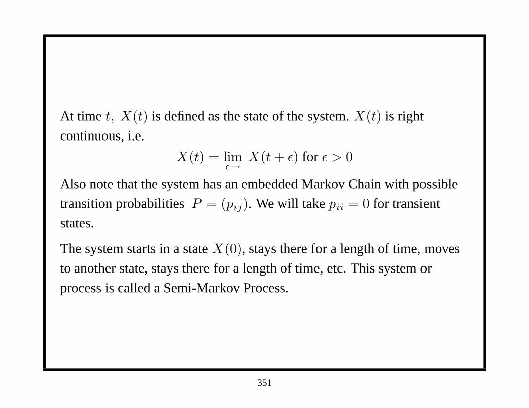
At time t, X(t) is defined as the state of the system. X(t) is right

continuous, i.e.

X(t) = limε→

X(t + ε) for ε > 0

Also note that the system has an embedded Markov Chain with possible

transition probabilities P = (pij). We will take pii = 0 for transient

states.

The system starts in a state X(0), stays there for a length of time, moves

to another state, stays there for a length of time, etc. This system or

process is called a Semi-Markov Process.

351

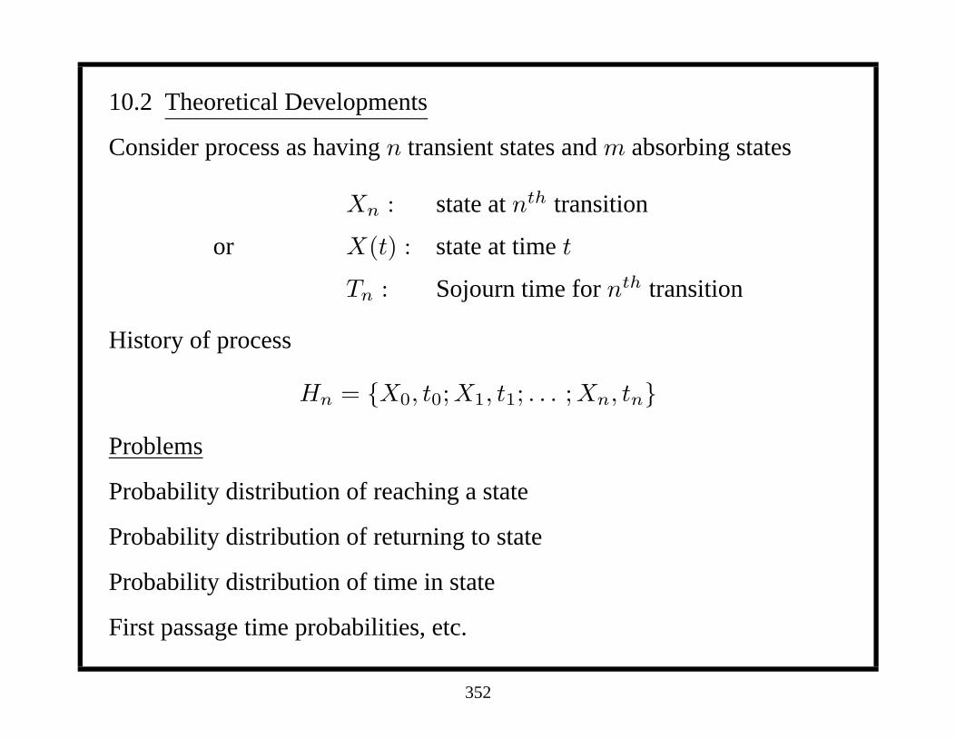
10.2 Theoretical Developments

Consider process as having n transient states and m absorbing states

Xn : state at nth transition

or X(t) : state at time t

Tn : Sojourn time for nth transition

History of process

Hn = {X0, t0; X1, t1; . . . ; Xn, tn}

Problems

Probability distribution of reaching a state

Probability distribution of returning to state

Probability distribution of time in state

First passage time probabilities, etc.

352

Assume:

P{Xn = j, t < Tn ≤ t+∆t|Hn−1} = P{Xn = j, t < Tn ≤ t+∆t|Xn−1}

Joint probability depends on History only through previous state

πij(t) = lim∆t→0

P (Xn = j, t < Tn ≤ t + ∆t|Xn−1 = i)

∆t

Since πij(t) does not depend on n (nth transition) the process is time

homogeneous.

pij =

∫ ∞

0

πij(t)dt = P{Xn = j|Xn−1 = i} i 6= j, where pii = 0

.̇. {Xn, n ≥ 0} form a Markov chain

P{t < Tn ≤ t + ∆t|Xn = j, Xn−1 = i} =πij(t)dt

pij

= qij(t)dt

353

qij(t) : pdf of sojourn time in state j conditional on coming from state i.

πij(t)dt = pijqij(t)dt

πij(t) = pijqij(t)

qij(t) is a pdf of time spent in j conditional on previous transition being

in i. qij(t) may be defined by:

qij(t) = qj(t)

qij(t) = qi(t)

qij(t) = q(t)

If qij(t) = λije−λijt the stochastic process is called a Markov Process.

Many authors define a Markov Process when λij = λj .

354

Remark: Sojourn time in state depends on current and previous state.

Note: Two Time Scales — Internal Time and External Time.

External Time: Time leaving or entering state

Internal Time: Time in a state or time to return to state

Def.

wij(t)dt = P{system leave state j during (t, t + dt)|X0 = i}

wij(t) is defined by external time

Nij(T ) =

∫ T

0

wij(t)dt = Expected no. of times system leaves state

j conditional on X0 = i over (0, T )

Nij = limT→∞

Nij(t)

= Expected no. of times system leaves state j over [0,∞)

conditional on X0 = i.

355

Definition:

qoi(t): pdf of time spent in the initial state X0 = i

qij(t): pdf of time spent in state j conditional on coming from state i.

Qoi(t) = P{T0 > t|X0 = i} =

∫ ∞

t

qoi(x)dx

Qij(t) = P{Tn > t, xn = j|x0 = i} =

∫ ∞

t

qij(x)dx

Def.: Uij(t) = P{system in state j at time t|X0 = i}

Uij(t) is a function of external time; qoi(t), qij(t) are functions of

internal time.

356

A. Finding Uij(t)

Suppose x0 = j. Then to be in j at time t either:

(a) system never left x0 = j

j>Time

t0Uii(t) = δijUij(t) = Q0i(t)δij

or

(b) system left state k at time τ (wi(τ)), entered state j (pkj) and stayed

at least (t− τ) units of time Qkj(t− τ); i.e. wik(τ)dτpkjQkj(t− τ).

Then integrate over possible values of τ (0, t) and sum over all transient

states

n∑

k=1

pkj

∫ t

0

wik(τ)Qkj(t− τ)dτ

357

Since (a) and (b) describe mutually exclusive events

Uij(t) = Q0i(t)δij +

n∑

k=1

pkj

∫ t

0

wik(τ)Qkj(t− τ)dτ

i, j = 1, 2, . . . , n

Taking LaPlace Transforms

U∗ij(s) = Q∗

oi(s)δij +

n∑

k=1

pkjw∗ik(s)Q∗

kj(s)

for i, j = 1, 2, . . . , n (only over transient states)

358

B. Finding wij(t)dt

If x0 = j then to leave state j in interval (t, t + dt) either:

(a) system never left state i before time t and emerged for first time at

(t, t + dt); i.e. P{t < T0 ≤ t + dt|x0 = j}

wii(t) = δijwij(t) = qoi(t)dtδij

or

(b) system leaves state k at time τ (wik(τ)dτ); enters state j (pkj) and

stays there for (t− τ, t− τ + dt) time units (qkj(t− τ)dt). Hence

wij(t)dt = qoi(t)dtδij +

n∑

k=1, k 6=j

pkj

∫ t

0

wik(τ)qkj(t− τ)dτdt

359

wij(t) = qoi(t)δij +

n∑

k=1

pkj

∫ t

0

wik(τ)qkj(t− τ)dτ

i, j = 1, 2, . . . , n

Taking Laplace Transforms

w∗ij(s) = q∗oi(s)δij +

n∑

k=1

pkjw∗ik(s)q∗kj(s)

i, j = 1, 2, . . . , n

Remark: The equations in the time domain are two sets of coupled

integral equations. However in the S domain, we have two sets of linear

equations.

360

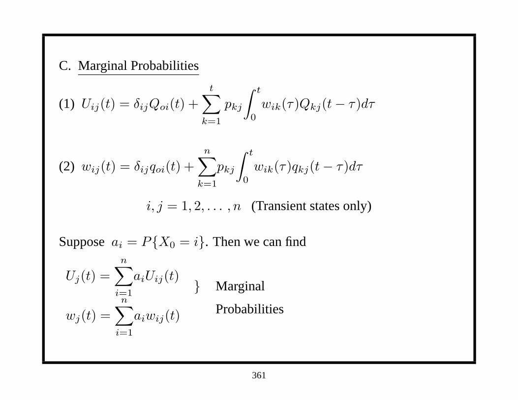
C. Marginal Probabilities

(1) Uij(t) = δijQoi(t) +

t∑

k=1

pkj

∫ t

0

wik(τ)Qkj(t− τ)dτ

(2) wij(t) = δijqoi(t) +

n∑

k=1

pkj

∫ t

0

wik(τ)qkj(t− τ)dτ

i, j = 1, 2, . . . , n (Transient states only)

Suppose ai = P{X0 = i}. Then we can find

Uj(t) =

n∑

i=1

aiUij(t)

wj(t) =n∑

i=1

aiwij(t)

} Marginal

Probabilities

361

Multiplying (1) by ai and summing over i

Uj(t) =

n∑

i=1

δijaiQoi(t) +

n∑

k=1

pkj

∫ t

0

wk(τ)Qkj(t− τ)dτ

Sincen∑

i=1

δijaiQoi(t) = ajQoj(t)

Uj(t) = ajQoj(t) +n∑

k=1

pkj

∫ t

0

wk(τ)Qkj(t− τ)dτ, j = 1, 2, . . . , n

Similarly

wj(t) = ajqoj(t) +n∑

k=1

pkj

∫ t

0

wk(τ)qkj(t− τ)dτ, j = 1, 2, . . . , n

w∗i = D(q∗0)ei + π∗′

w∗i

362

Consider n = 3 and i = 2

w∗i1(s)

w∗i2(s)

w∗i3(s)

=

q∗01(s) 0 0

0 q∗02(s) 0

0 0 q∗03(s)

0

1

0

+

0 p21q∗21(s) p31q

∗31

p12q∗12(s) 0 p32q

∗32

p13q∗13(s) p23q

∗23(s) 0

w∗i1

w∗i2

w∗i3

w∗i =

∑3j=1 pj1q

∗j1(s)w

∗2j(s)

q∗02(s) +∑3

j=1 pj2q∗j2(s)w

∗2j(s)

∑3j=1 pj3q

∗j3(s)w

∗2j(s)

Similarly Ui = D(Q∗0)ei + Φ∗′

w∗i

363

D. Matrix Relations and Solutions

Consider the S - domain equations:

U∗ij(s) = Q∗

oi(s)δij +

n∑

k=1

pkjw∗ik(s)Q∗

kj(s)

w∗ij(s) = q∗oi(s)δij +

n∑

k=1

pkjw∗ik(s) q∗kj(s)

364

Define:

U∗i = (U∗

i1(s), U∗i2(s), . . . , U∗

in(s))′

w∗i = (w∗

i1(s), . . . , w∗in(s))′

Q∗o = (Q∗

o1(s), . . . , Q∗on(s))′

P = (pij), Φ∗ij(s) = pijQ

∗ij(s), Φ∗ = (Φ∗

ij)

π∗ij(s) = pijq

∗ij(s), π∗ = (πij(s))

ei = (0, 0, . . . , 1, 0 . . . 0)′ 1 in ith position

⇒U∗

i = D(Q∗0)ei + Φ∗′

w∗i

w∗i = D(q∗0)ei + π∗′

w∗i

w∗i = D(q∗0)ei + π∗′

w∗

(I − π∗′

)w∗i = D(q∗o)ei

365

Def. N∗ = (I − π∗′

)−1

w∗i = (I − π∗′

)−1D(q∗0)ei = N∗D(q∗0)ei

w∗ij(s) =

∫ ∞

0

e−stwij(t)dt

w∗ij(0) =

∫ ∞

0

wij(t)dt =Expected no. of visits to j

conditional on x0 = i

.̇. putting s = 0 in: w∗i , D(q∗0), N∗

w∗i (0) = N∗(0)ei as q∗0i(0) = 1, N∗(0) = (I − P ′)−1

i.e.

N∗(0) = [I − π∗′

(0)]−1 , π∗(s) = (pijq∗ij(s))

π∗(0) = P, π∗(0)′ = P ′

.̇. N(0) = (I − P ′)−1

366

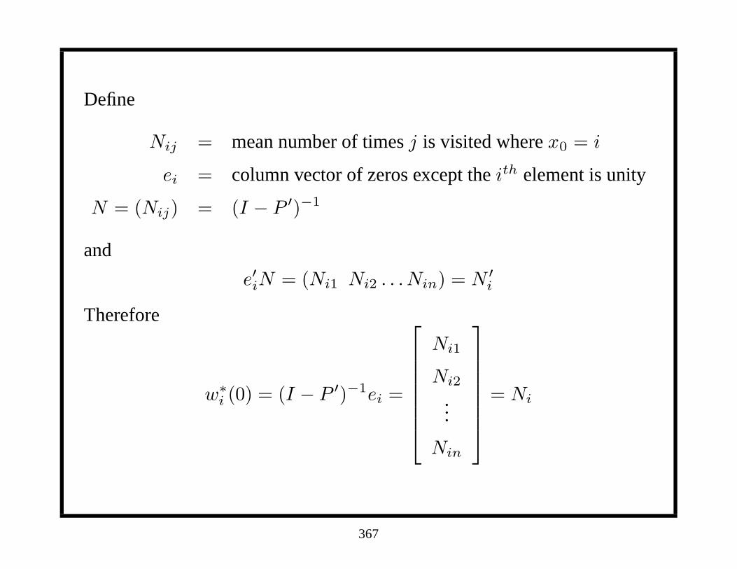
Define

Nij = mean number of times j is visited where x0 = i

ei = column vector of zeros except the ith element is unity

N = (Nij) = (I − P ′)−1

and

e′iN = (Ni1 Ni2 . . . Nin) = N ′i

Therefore

w∗i (0) = (I − P ′)−1ei =

Ni1

Ni2

...

Nin

= Ni

367

w∗i = N∗D(q∗0)ei

U∗i = D(Q∗

0)ei + Φ′∗w∗i , Φ∗(pijQ

∗ij(s))

= D(Q∗0)ei + Φ′∗N∗D(q∗0)ei

U∗i = [D(Q∗

0) + Φ′∗N∗D(q∗0)]ei

Recall: U∗ij(s) =

∫ ∞

0

Uij(t)e−stdt

U∗ij(0) =

∫ ∞

0

Uij(t)dt = mean time spent in j conditional on X0 = i

Q∗oi(0) =

∫ ∞

0

Qoi(t)dt = moi

Φ∗(s) = (pijQ∗ij(s)), Φ

∗(0) = (pijmij), where mij is mean of qij(t).

368

Ex. n = 3, X0 = 2, e2 = (0 1 0)′

U∗2 (0) = [D(m0) + Φ′∗(0)N∗(0)]e2

U∗21(0)

U∗22(0)

U∗23(0)

=

m01 0 0

0 m02 0

0 0 m03

0

1

0

+

0 p21m21 p31m31

p12m12 0 p32m32

p13m13 p23m23 0

N21

N22

N23

as N∗(0)ei =

N11 N21 N31

N12 N22 N32

N13 N23 N33

0

1

0

=

N21

N22

N23

369

U∗21(0)

U∗22(0)

U∗23(0)

=

0

m02

0

+

3∑

j=1

pj1mj1N2j

3∑

j=1

pj2mj2N2j

3∑

j=1

pj3mj3N2j

=mean time in state j = 1,2,3

starting from X0 = 2

370

Interpretation

U∗21(0) =

3∑

j=1

pj1mj1N2j = mean time spent in state 1 if X0 = 2.

mj1N2j = (meantime in 1 coming from j)

×(Expected no. of visits from 2 to j)

pj1mj1N2j = E[Total no. of visits to j starting from state 2]

×Probability {j → 1}

×mean time in state 1 coming from j

U∗22(0) = m02 +

3∑

j=1

pj2mj2N2j

Note additional term because X0 = 2.

371

Homework

Consider the 3 state model with transition probabilities

P =

0 α 1− α

β 0 1− β

0 0 1

States 1 and 2 are transient states and state 3 is an absorbing state.

Define qij(t) = qj(t) = λje−λjt

Find Uij(t) and wij(t) for i, j = 1, 2.

372

E. Matrix Note

All results depended on the inversion of [I − π∗′

ij (s)]. Does inverse exist?

Consider matrix (n× n) A.

Ln = (I −A)(I + A + A2 + . . . + An−1)

= (I + A + . . . + An−1)− (A + A2 + . . . + An) = I −An

If An → 0 as n→∞⇒ Ln → I and (I −A)−1 = I + A + A2 + . . .

exists.

Now consider (I − π∗′

), π∗ = (π∗ij) = (pijq

∗ij(s))

Since q∗ij(s) =

∫ ∞

0

e−stqij(t)dt, |q∗ij(s)| ≤ 1 .̇. |π∗ij | ≤ pij

But Pn = (p(n)ij )→ 0 as n→ 0 as there exists at least one absorbing

state and with prob = 1, system will eventually be in absorbing state.

373

10.3 Simplified Model

Suppose qij(t) = qj(t) and q0j(t) = q(j(t); i.e. sojourn time only

depends on the state process is in. Then

πij(t) = pijqij(t) = pijqj(t)

Φij(t) = pijQij(t) = pijQj(t)

π(t) = πij(t)) =

0 p12q2(t) p13q3(t) . . . p1nqn(t)

p21q1(t) 0 p23q3(t) . . . p2nqn(t)...

pn1q1(t) pn2q2(t) . . . 0

374

π(t) = PD(q), D(q) =

and π∗ = PD(q∗)

q1(t) 0 . . . 0

0 q2(t) . . . 0...

0 . . . qn(t)

Similarly Φ(t) = PD(Q), Φ∗(s) = PD(Q∗)

π∗ = PD(q∗), Φ∗ = PD(Q∗)

D(q∗0) = D(q∗), D(Q∗0) = D(Q∗)

Since w∗i = (I − π′∗)−1D(q∗0)ei

we can write

w∗i = [I −D(q∗)P ′]−1D(q∗)ei

375

Consider[I −D(q∗)P ′]−1D(q∗) = [I + DP ′ + (DP ′)2 + . . . ]D

= D[I + P ′D + (P ′D)2 + . . . ]

= D∗(q∗)[I − P ′D(q∗)]−1 = D(q∗)M∗

where M∗ = [I − P ′D(q∗)]−1

.̇. w∗i = D(q∗)M∗ei

Similarly

U∗i = D(Q∗

0)e∗i + Φ′∗w∗

i

= D(Q∗)ei + D(Q∗)P ′D(q∗)M∗ei

= D(Q∗)[I + P ′D(q∗)M∗]ei

376

U∗i = D(Q∗)[I + P ′D(q∗)M∗]ei

where M∗ = [I − P ′D(q∗)]−1

But P ′DM∗ = P ′D[I − P ′D]−1 = P ′D[I + P ′D + (P ′D)2 + . . . ]

P ′DM∗ = P ′D + (P ′D]2 + (P ′D]3 + . . .

= [I − P ′D]−1 − I = M∗ − I

.̇. U∗i = D(Q)∗M∗ei

.̇. When the sojourn time only depends on the state the process is in we

also have

w∗i = D(q∗)M∗ei .

377

Then w∗i (0) = (I − P ′)−1ei =

Ni1

Ni2

...

Nin

= Ni

U∗i (0) = D(m)Ni =

m1 0

m2

0. . .

mn

Ni1

Ni2

...

Nin

=

m1 Ni1

m2 Ni2

...

mn Nin

378

First Passage Time Problems

A. Time from X0 = i to being absorbed

To simplify the problem, suppose that there is only one absorbing state

which is n + 1.

Define Ti = random variable to Absorption conditional on X0 = i.

Gi(t) = P{Ti > t|X0 = i} = P{TX0> t|X0 = i}

Ui,n+1(t) = Prob. system is in state n + 1 at time t.

1− Ui,n+1(t) = Prob. system is not in (n + 1) at t

⇒ Gi(t) = 1− Ui,n+1(t) =

n∑

k=1

Uik(t)

asn∑

k=1

Uik(t) + Ui,n+1(t) = 1

379

Gi(t) =n∑

k=1

Uik(t)

G∗i (s) =

n∑

k=1

U∗ik(s)

Since G∗i (0) =

∫ ∞

0

Gi(t)dt =

n∑

j=1

U∗ij(0) = mean time to Absorption

But we had found

U∗ij(0) = mean time in j starting from X0 = i

= δijmoi +

n∑

k=1

pkjmkjNik

.̇. G∗i (0) =

n∑

j=1

n∑

k=1

pkjmkjNik + moi

380

If mkj = mj ,

G∗i (0) =

n∑

j=1

mj

n∑

k=1

pkjNik + moi

Recall

w∗ij(s) = q∗oi(s)δij +

n∑

k=1

pkjw∗ik(s)q∗kj(s)

w∗ij(0) = δij +

n∑

k=1

pkjw∗ik(0)

or equivalently Nij =n∑

k=1

pkjNik i 6= j

Nii = 1 +n∑

k=1

pkiNik

G∗i (0) =

n∑

j=1

mj

n∑

k=1

pkjNik + moi

381

If mkj = mj

Nij =n∑

k=1

pkjNik i 6= j

Nii = 1 +

n∑

k=1

pkjNik

.̇. G∗i (0) =

n∑

j=1,j 6=i

mj

[

n∑

k=1

pkjNik

]

+ mi

n∑

k=1

pkiNii + moi

=∑

j 6=i

mjNij + mi[Nii − 1] + moi

G∗i (0) =

n∑

j=1

mjNij + (moi −mi)

If moi = mi, G∗i (0) =

n∑

j=1

mjNij

382

B. Variance of Time to Absorption

G∗i (s) =

n∑

j=1

U∗ij(s), Gi(t) = P{Ti > t|X0 = i}

If gi(t) is pdf of time to Absorption with X0 = i, we know that

G∗i (s) =

1− g∗i (s)

s=

1− [1− sm1 +s2

2m2 + · · · ]

s= m1 −

s

2m2 + O(s2)

dG∗i (s)

ds= −

m2

2+ O(s)

and taking s = 0 ⇒ m2 = −2

(

dG∗i (s)

ds

)

s=0

.̇. V ar Ti = m2 −m21 = −2G∗

i (0)− [G∗i (0)]2

We have found G∗i (0), it is only necessary to find −2

dG∗t (s)

dsevaluated at

s = 0

383

To simplify problem we will consider the special case

mkj = mj , moj = mj

Then

U∗i = D(Q∗)M∗ei, M∗ = [I − P ′D(q∗)]−1

−2dU∗

i

ds= −2

d

dsD(Q∗)M∗ei − 2D(Q∗)

dM∗

dsei

Recall −2dQ∗

j (s)

ds=second moment of qj(t) = (σ2

j + m2j ), s = 0

.̇. −2d

dsD(Q∗)s=0 = D(σ2+m2) =

σ21 + m2

1

σ22 + m2

2 0

0. . .

σ2k + m2

k

384

To evaluatedM∗

ds, consider M∗M∗−1

= I

dM∗

dsM∗−1

+ M∗ d

dsM∗−1

= 0

dM∗

ds= −M∗

(

d

dsM∗−1

)

M∗

Since M∗−1

= I − P ′D(q∗),

(

dM∗−1

ds

)

s=0

= +P ′D(m)

dM∗

ds= −M∗

(

d

dsM∗−1

)

M∗

and setting s = 0(

dM∗

ds

)

0

= −(I − P ′)−1P ′D(m)(I − P ′)−1 = −NP ′D(m)N

385

.̇. − 2dU∗

i

ds=

[

−2d

dsD(Q∗)M∗, − 2D(Q∗)

dM∗

ds

]

ei

Setting s = 0

= [D(σ2 + m2)N + 2D(m)NP ′D(m)N ]ei

Now Nei =

Ni1

Ni2

...

Nik

−2dU∗

i

ds= [D(σ2 + m2) + 2D(m)NP ′D(m)]Ni

Also G∗i (0) =

∑

U∗i (0) =

N∑

1

Nimi = N ′im

386

.̇. V arTi = −2∑

(

dU∗i (s)

ds

)

s=0

−m′NiN′im

=

n∑

j=1

σ2j Nij +

N∑

j

m2jNij + 2m′[N − I]D(m)Ni −m′NiN

′im

as NP ′ = (I − P ′)−1P ′ = P ′ + P ′2 + . . . = N − I

.̇. V arT0 =∑

σ2j Nij +

∑

j

m2jNij +2m′[N−I]D(m)Ni−m′NiN

′im

Simplifying m′[N − I]D(m)Ni

387

D(m)Ni = D(Ni)m

m′[N − I]D(m)Ni = m′ND(Ni)m−m′D(Ni)m

Note: m′D(Ni)m =

n∑

j=1

m2jNij

V arTi =∑

σ2j Nij + 2m′ND(Ni)m−

∑

j m2jNij

−m′NiN′im

=∑

j σ2j Nij + m′[2N − I]D(Ni)m−m′NiN

′im

V arTi =∑

j

σ2j Nij + m′{[2N − I]D(Ni)−NiN

′i}m

388

C. Time to go from any state j to being absorbed conditional on X0 = i

Earlier we had found the prob. distribution of being absorbed starting out

from X0 = i at time 0.

Now we wish to generalize the result of finding the time to Absorption for

an arbitrary state j with X0 = i.

Define

gj,n+1(t) = gj(t) = pdf of time to being absorbed beginning with the

time the system enters state j.

389

There are two ways of going from j to the absorbing state n + 1; i.e.

(a) The state after j is the absorbing state. Hence the time to beingabsorbed is Tj (time spent in j), or(b) The state after j is another transient state r and the time to beingabsorbed is Tj + Tr,n+1 where Tr,n+1 is the time to Absorption fromstate r.Assume that the state prior to entering state j is state k.

gj,n+1(t) = gj(t)

=

n∑

k=1

pkjqkj(t)pj,n+1 +

n∑

k=1

n∑

r=1

pkj

∫ t

0

qkj(τ)pjrgr(t− τ)dτ

gj(t) = pj,n+1qj(t) +

n∑

r=1

pjr

∫ t

0

qj(τ)gr(t− τ)dτ

where qj(t) =

n∑

k=1

pkjqkj(t)

390

gj(t) = pj,n+1qj(t) +

n∑

r=1

pjr

∫ t

0

qj(τ)gr(t− τ)dτ j = 1, . . . , n

where qj(t) =

n∑

k=1

pkjqkj(t).

Note that before entering j the process was in state k. Thus the pdf of thestay in j is qkj(t). However it came from state k with prob. pkj . It is alsonecessary to sum over all possible values of k. This leads to the marginaldistribution qj(t).

Taking LaPlace Transforms results in

g∗j (s) = pj,n+1q∗j (s) +

n∑

r=1

pjrq∗j (s)g∗r (s)

for j = 1, . . . , n.

391

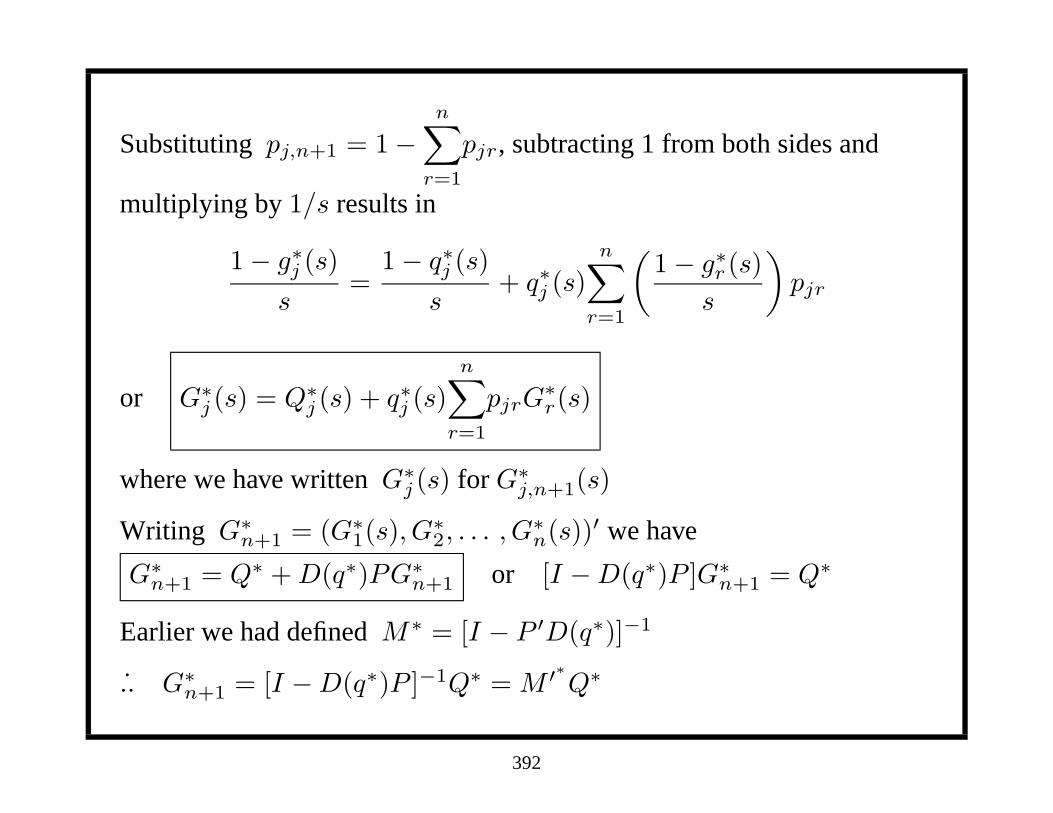
Substituting pj,n+1 = 1−

n∑

r=1

pjr, subtracting 1 from both sides and

multiplying by 1/s results in

1− g∗j (s)

s=

1− q∗j (s)

s+ q∗j (s)

n∑

r=1

(

1− g∗r (s)

s

)

pjr

or G∗j (s) = Q∗

j (s) + q∗j (s)

n∑

r=1

pjrG∗r(s)

where we have written G∗j (s) for G∗

j,n+1(s)

Writing G∗n+1 = (G∗

1(s), G∗2, . . . , G∗

n(s))′ we have

G∗n+1 = Q∗ + D(q∗)PG∗

n+1 or [I −D(q∗)P ]G∗n+1 = Q∗

Earlier we had defined M∗ = [I − P ′D(q∗)]−1

.̇. G∗n+1 = [I −D(q∗)P ]−1Q∗ = M ′∗Q∗

392

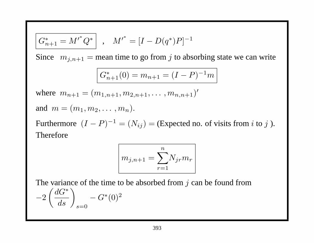
G∗n+1 = M ′∗Q∗ , M ′∗ = [I −D(q∗)P ]−1

Since mj,n+1 = mean time to go from j to absorbing state we can write

G∗n+1(0) = mn+1 = (I − P )−1m

where mn+1 = (m1,n+1, m2,n+1, . . . , mn,n+1)′

and m = (m1, m2, . . . , mn).

Furthermore (I − P )−1 = (Nij) = (Expected no. of visits from i to j ).

Therefore

mj,n+1 =

n∑

r=1

Njrmr

The variance of the time to be absorbed from j can be found from

−2

(

dG∗

ds

)

s=0

−G∗(0)2

393

D. First passage time to go from X0 = i to an arbitrary Absorption state

Consider n transient states and m absorbing states. The transient states

will be written as the first n states. Assume X0 = i and it is desired to

find the first passage time starting from X0 = i to being absorbed by state

r, conditional on reaching state r.

Define

fir = Prob. of being absorbed by state r

conditional on X0 = i

fir = pir +

n∑

j=1

pijpjr +∑

j,k

pikpkjpjr +∑

j,k,l

pilplkpkjpjr

= pir +∑

j

pijpjr +∑

j

p(2)ij pjr +

∑

j

p(3)ij pjr + . . .

394

fir = pir +

n∑

j=1

pijpjr +∑

j

p(2)ij pjr +

∑

j

p(3)ij pjr + . . .

where p(m)ij = Prob. of i→ j in m steps

p(m)ij is i, jth element of P m.

Hence if fr = (f1r, f2r, . . . , fnr)′

R = (p1r, p2r, . . . , pnr)′

P = (pij) i, j = 1, 2, . . . , n

fr = R + PR + P 2R + . . . = (I + P + P 2 + . . . )R

fr = (I − P )−1R i.e. fir =

n∑

j=1

Nijpjr

fir = e′i(I − P )−1R = R′(I − P ′)−1ei

e′i(I − P )−1 = (Ni1, Ni2, . . . , Nim)

395

Define

gir(t) : pdf of time to being absorbed in state r with X0 = i,

and conditional on being absorbed in state r.

gir(t) =

n∑

j=1

wij(t)pjr/fir = w′i(t)R/fir

where wi(t) = (wi1(t), wi2(t), . . . , win(t))′

R = (p1r, p2R, . . . , pnr)′

g∗ir(s) = w∗i (s)′R/fir = R′w∗

i (s)/fir

where w∗i (s) = N∗D(q∗0)ei

Note: g∗ir(0) =R′w∗

i (0)

fir

=

n∑

j=1

Nijpjr

fir

= 1

396

E. Other First Passage Time Problems

1. Suppose i, j ∈ T (T= Transient States)

Define T ′ = (n− 1) transient states omitting j. A is set of absorbing

states.

fij = Prob. of i→ j (Probability of eventually reaching j from i)

fij = pij +∑

k∈T ′

pikpkj +∑

k,l∈T ′

pikpklplj + . . . .

Partition the transition matrix P

P =

T ′ j A

T ′ P̄ α γ α′ = (p1j , p2j , . . . , pnj)

j β′ 0 δ , omit pjj

A 0 0 I β′ = (pj1, pj2, . . . , pjn)

397

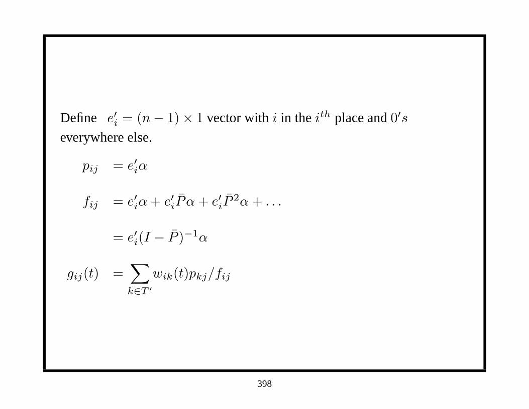
Define e′i = (n− 1)× 1 vector with i in the ith place and 0′s

everywhere else.

pij = e′iα

fij = e′iα + e′iP̄α + e′iP̄2α + . . .

= e′i(I − P̄ )−1α

gij(t) =∑

k∈T ′

wik(t)pkj/fij

398

2. First passage time to return to j

gjj(t) =∑

k∈T ′

wjk(t)pkj/fjj

fjj = Prob. of visiting j after initial visit

fjj =∑

k∈T ′

pjkpkj +∑

k,l,∈T ′

pjkpklplj + . . .

fjj = β′α + β′P̄α + β′P̄ 2α + . . . = β′(I − P̄ )−1α

399

10.5 Alternate Model: Semi-Markov II

Suppose time in state depends on current state and the next state. Ourmodels up to now have assumed time in state depends on current state andstate before current state; i.e.

P{t < TXn≤ t + dt, Xn = j|Xn−1 = i} = πij(t)dt.

Now assume

P{t < TXn≤ t + dt, Xn+1 = j|Xn = i} = πij(t)dt

P{t < TXn≤ t + dt|Xn = i, Xn+1 = j} = qij(t)dt

πij(t) = pijqij(t)

qij(t): refers to the pdf of time in i where j is the next transition.

400

Suppose X0 = i. If next state is k, then time spent in i is q(0)ik (t) where

the (0) indicates the initial state with probabiblity pik.

Define Uij(t), wij(t) as before where i, j ∈ Transient states.

Uij(t) =

[

n∑

k=1

pikQ(0)ik (t)

]

δij

+

n∑

k=1

n∑

l=1

∫ t

0

wik(τ)pkjQjl(t− τ)pjldτ

Initial state X0 = i: If j = i, δij = 1 and Q0ik(t) where k is next state

with Prob. = pik.

Other: At time t, system is in state j. Hence at time < t, it entered j froma state k and left state k at time τ(τ < t). Also the state after j is l withProb. p

jl.

401

Uij(t) =

[

n∑

k=1

pikQ(0)ik (t)

]

δij +

n∑

k=1

pkj

∫ t

0

wik(τ)

[

n∑

l=1

pjlQjl(t− τ)

]

dτ

Define

Qi0(t) =n∑

k=1

pikQ(0)ik (t) Qj(t) =

∑

l=1

pjlQjl(t)

Then Uij(t) = δijQi0(t) +

n∑

k=1

pkj

∫ t

0

wik(τ)Qj(t− τ)dτ

These are same equations as our other model except the sojourn time needonly be marginal distributions.

Taking LaPlace Transforms

U∗ij(s) = δijQ

∗i0(s) + Q∗

j (s)

n∑

k=1

pkjw∗ik(s)

402

Similarly we have

wij(t) = δijqi0(t) +∑

k

pkj

∫ t

0

wik(τ)qj(t− τ)dτ

resulting in

wij(s) = δijq∗i0(s) + q∗j (s)

n∑

k=1

pkjw∗ik(s)

Hence in matrix notation

w∗i = D(q∗0)ei + D(q∗)P ′w∗

i

[I −D(q∗)P ′]w∗i = D(q∗0)ei

w∗i = N∗D(q∗0)ei), N∗ = [I −D(q∗)P ′]−1

403

w∗i = N∗D(q∗0)ei), N∗ = [I −D(q∗)P ′]−1

U∗ij(s) = δijQ

∗io(s) + Q∗

j (s)

n∑

k=1

pkjw∗ik(s)

or in matrix notation U∗i = D(Q∗

0)ei + D(Q∗)P ′w∗i

Substituting for w∗

U∗i = D(Q∗

0)ei + D(Q∗)P ′N∗D(q∗0)ei

Now if Q∗0i(s) = Q∗

i (s)

U∗i = [D(Q∗) + D(Q∗)P ′N∗D(q∗)]ei

U∗i = D(Q∗)[I + P ′N∗D(q∗)]ei

404

SinceP ′N∗D(q∗) = P ′[I + DP ′ + (DP ′)2 + . . . ]D

= P ′D + (P ′D)2 + . . . = (I − P ′D)−1 − I = M∗ − I

U∗i = D(Q∗)M∗ei, M∗ = [I − P ′D(q∗)]−1

U∗i = D(Q∗)M∗ei , M∗ = [I − P ′D(q∗)]−1

Now

w∗i = N∗D(q∗0)ei , N∗ = [I −D(q∗)P ′]−1

Consider

N∗D = [I + DP ′ + (DP ′)2 + . . . ]D

= D[I + P ′D + . . . ] = D(I − P ′D)−1

N∗D(q∗) = D(q∗)M∗

Therefore w∗i = D(q∗)M∗ei when q∗0i = q∗i

405