semmes family of curves and a characterization of...
TRANSCRIPT
Semmes family of curves and a characterization offunctions of bounded variation in terms of curves ∗
Riikka Korte, Panu Lahti and Nageswari Shanmugalingam†
September 1, 2013
Abstract
On metric spaces supporting a geometric version of a Semmes family of curves, weprovide a Reshetnyak-type characterization of functions of bounded variation in termsof the total variation on such a family of curves. We then use this characterizationto obtain a Federer-type characterization of sets of finite perimeter, that is, we showthat a measurable set is of finite perimeter if and only if the Hausdorff measure of itsmeasure theoretic boundary is finite. We present a construction of a geometric Semmesfamily of curves in the first Heisenberg group.
1 Introduction
Research on analysis in metric measure spaces, a field that has seen much recent activity, hasproduced various analogs of the Sobolev spaces of functions W 1,p(Ω), where Ω is a Euclideandomain. As expected from the behavior of the classical Sobolev spaces, the behavior of thesespaces is significantly different for p = 1 than for p > 1. It is well-known that the relaxation ofthe space W 1,1(Ω) is associated with the more geometric objects called functions of boundedvariation, denoted BV (Ω). Using this observation, a theory of functions of bounded variationwas developed in [Mir], [Am1], [Am2] and [AMP] in the setting of metric spaces equippedwith a doubling measure.
Surprisingly, the theory of functions of bounded variation plays a role in the study of theanalogs of the Sobolev classes W 1,p
0 (Ω), p > 1, of functions with zero boundary values in sucha metric setting. In [KKST] it was first shown that a so-called strong relative isoperimetricinequality is equivalent with a Federer-type characterization of sets of finite perimeter, thatis, sets whose characteristic functions are functions of bounded variation. According to
∗2000 Mathematics Subject Classification: Primary 31E05; Secondary 26A45, 26B30, 30L99.Keywords : BV, sets of finite perimeter, Federer characterization, Semmes family of curves, Poincare inequal-ity, Newtonian spaces, metric measure spaces.†We thank Riikka Kangaslampi for illuminating conversations on the geometry of geodesics in the
Bourdon-Pajot spaces. We also thank Luigi Ambrosio and Juha Kinnunen for their encouragement withthis project. R. K. was partially supported by Academy of Finland, grant #250403. P. L. was supportedby the Finnish Academy of Science and Letters, the Vilho, Yrjo and Kalle Vaisala Foundation. N. S. waspartially supported by NSF grants DMS-0355027 and DMS-1200915.
1

the Federer-type characterization, a set has finite perimeter if and only if the codimension 1Hausdorff measure of its measure theoretic boundary is finite. In verifying a characterizationof the analogs of Sobolev functions with zero boundary values on a domain in the metricmeasure space, it was shown in [KKST] that this Federer-type characterization allows us toeliminate the overly restrictive assumption of finiteness of a codimension 1 Hausdorff measureof the topological boundary of the domain. In the Euclidean setting it is well-known thatsets whose measure theoretic boundaries are of finite codimension 1 Hausdorff measure areof finite perimeter. This fact was first proved by Federer in [Fed], and a simplified versionof the proof can be found in [EvGa]. A weaker version of the result is proved in [KL] inthe setting of a metric space equipped with a doubling measure and supporting a Poincareinequality.
The proof of the Federer-type characterization in the Euclidean setting uses a Reshetnyak-type characterization of functions of bounded variation in terms of the total variation of thefunction restricted to lines parallel to a coordinate axis. An analogous characterization ofSobolev functions, involving absolute continuity on lines, holds in the Euclidean setting, seefor example [Zie], [Vai] and [Oht]. This characterization has been used in [Shan] and [HKST]to construct an analog of Sobolev classes of functions in the metric measure space setting;such classes of functions, called the Newtonian spaces N1,p, have been used extensively tostudy potential theory and quasiconformal mappings. In the metric setting, a Reshetnyak-type characterization involving all curves in the space has been established for BV functions,see [AmDi]. However, it is unclear how to proceed from this to the Federer-type character-ization. The point of the present work is to show that if a doubling metric measure spacesupports a geometric version of a Semmes family of curves originally presented in [Sem],then measurable sets whose measure theoretic boundaries have finite codimension 1 Haus-dorff measure are necessarily of finite perimeter in the sense of [Mir] and [Am2]. One ofthe simplest non-Euclidean metric measure spaces, the first Heisenberg group, appears tosupport a geometric Semmes family of curves.
This paper is organized as follows. Section 2 will contain the basic definitions and notationused throughout the paper, and in Section 3 we discuss the notion of a Semmes family ofcurves and its additional geometric properties. In Section 4 we provide a Reshetnyak-typecharacterization of functions of bounded variation in terms of the total variation of a functionon curves belonging to the geometric Semmes family. In Section 5 we proceed to give a proofof the Federer-type characterization of sets of finite perimeter, by means of the Reshetnyak-type characterization. Section 6 contains examples of metric measure spaces that supporta geometric Semmes family of curves, including Euclidean spaces and Fred Gehring’s bow-tie. In particular, we present a construction of the geometric Semmes family in the firstHeisenberg group.
2 Preliminaries
2.1 Notation and assumptions
We assume throughout that X = (X, d, µ) is a metric measure space equipped with a metricd and a Borel regular, doubling outer measure µ. The doubling property means that there
2
is a fixed constant cd ≥ 1, called the doubling constant of µ, such that
µ(2B) ≤ cd µ(B) (2.1)
for every ball B = B(x, r) := y ∈ X : d(y, x) < r. Here tB = B(x, tr), and we also denoter =: rad(B). We note that in a metric space, balls do not necessarily have unique centersor radii, but we assume each ball to have a prescribed center point and radius. We assumethat the measure of every open set is positive and that the measure of every bounded setis finite. The doubling condition implies that for every x ∈ X, every 0 < r ≤ R < ∞ andevery y ∈ B(x,R), we have
µ(B(y, r))
µ(B(x,R))≥ c
( rR
)Q(2.2)
for some constants c > 0 and Q > 0, which only depend on the doubling constant cd. We alsoassume the space to be connected, which is implied by the Poincare inequality (see (2.10)),and which in turn implies that µ(x) = 0 for every x ∈ X (we assume that X is not aone-point space). The Poincare inequality also implies that necessarily Q ≥ 1.
We further assume that X is complete; recall that a metric space with a doubling measureis complete if and only if the space is proper, that is, closed and bounded sets are compact.Since X is proper, for any open set Ω ⊂ X we define local spaces as follows: e.g. Liploc(Ω)is the space of functions that are Lipschitz in every open Ω′ b Ω. Here Ω′ b Ω means thatΩ′ is a compact subset of Ω. The support of a function u on X is denoted supp(u).
The integral average of a function u ∈ L1(A) over a µ-measurable set A with finite andpositive measure is uA :=
∫Au dµ := µ(A)−1
∫Au dµ. The characteristic function of a set
E ⊂ X is denoted χE. In general, C will denote a positive constant whose value is notnecessarily the same at each occurrence. When a constant C depends on e.g. the numbersa and b, it will be denoted C(a, b). When we say that a property holds for µ-almost everyx, y ∈ X, we mean that there is a set E ⊂ X such that µ(E) = 0 and the property holdsfor every x, y ∈ X \ E. We use the abbreviation “a.e.” for “almost every” or “almosteverywhere”.
We recall that because µ is doubling, for every locally integrable function u ∈ L1loc(X),
µ-a.e. point x ∈ X is a Lebesgue point, meaning that
limr→0
∫B(x,r)
|u− u(x)| dµ = 0.
See [Hei, Theorem 1.8] for a proof of this fact. Furthermore, for every µ-measurable functionu that is finite valued µ-a.e., µ-a.e. point is a point of approximate continuity (see e.g. [EvGa,Section 1.7.2]). This means that for every ε > 0,
limr→0
µ(B(x, r) ∩ |u− u(x)| ≥ ε)µ(B(x, r))
= 0.
Each Lebesgue point of u is clearly a point of approximate continuity, and the converse holdswhen u is essentially bounded.
Given two sets A1, A2 ⊂ X, the distance dist(A1, A2) is defined by
dist(A1, A2) := infd(x, y) : x ∈ A1, y ∈ A2,
3
whereas the Hausdorff distance is defined by
dH(A1, A2) := inf
ε > 0 : A1 ⊂
⋃x∈A2
B(x, ε) and A2 ⊂⋃x∈A1
B(x, ε)
.
A curve is a rectifiable continuous mapping from a compact interval into X. The lengthof a curve γ is denoted `γ or `(γ). We will assume that all curves are parametrized by arclength; such re-parametrization can always be done because γ is rectifiable (see e.g. [Haj] or[AT]). The image of a curve γ in X is also denoted γ. A curve γ′ is a subcurve of a curve γif γ′ is, after reparameterization, equal to γ|[a,b] for some 0 ≤ a < b ≤ `γ.
A nonnegative Borel function g on X is an upper gradient of an extended real valuedfunction u on X, if for all curves γ in X, we have
|u(x)− u(y)| ≤∫γ
g ds (2.3)
whenever both u(x) and u(y) are finite, and∫γg ds = ∞ otherwise. Here x and y denote
the end points of γ.Next we recall the definition of functions of bounded variation on metric spaces, given
by Miranda in [Mir].
Definition 2.4. For u ∈ L1loc(X), we define the total variation of u as
‖Du‖(X) := inf
lim infi→∞
infgui
∫X
gui dµ : ui ∈ Liploc(X), ui → u in L1loc(X)
,
where the second infimum in the above is over all upper gradients gui of ui. We say that afunction u ∈ L1
loc(X) is of bounded variation, u ∈ BV (X), if ‖Du‖(X) <∞. If the functionu is the characteristic function of a set E ⊂ X and ‖DχE‖(X) <∞, we say that the set Ehas finite perimeter. Similarly, we define ‖Du‖(Ω) for any open set Ω ⊂ X. If u ∈ BV (X),given an arbitrary set A ⊂ X (not necessarily open) we define
‖Du‖(A) := inf‖Du‖(Ω) : A ⊂ Ω,Ω is open.
According to [Mir], ‖Du‖(·) is then a finite Borel outer measure. For a set E, we also define
P (E,A) := ‖DχE‖(A),
which we call the perimeter of E in A.
When the space is taken to be the real line R and Ω is an interval (a, b), with −∞ ≤a < b ≤ ∞, we have a useful equivalent formulation for the variation measure. Namely, fora Lebesgue measurable function u, we have
‖Du‖((a, b)) = sup
l∑
n=1
|u(tn−1)− u(tn)|
, (2.5)
where the supremum is taken over all finite partitions a < t0 < . . . < tl < b such that eachtn is a point of approximate continuity of u, see e.g. [EvGa, Section 5.10.1]. For a Borelfunction u on X and curve γ, we use the notation
‖Dγu‖((0, `γ)) := ‖D(u γ)‖((0, `γ)).
4
Remark 2.6. In standard texts on real analysis (see for example [Roy] or [Rud]), the defi-nition of functions of bounded variation on an interval does not require the partitions tnto consist of points of approximate continuity. This type of definition is suitable if one workswith a particular L1-representative of each BV function. However, in our setting one canalways perturb a function on a set of measure zero without changing the total variation.
For any set A ⊂ X, the restricted spherical Hausdorff content of codimension 1 is definedas
HhR(A) := inf
∞∑i=1
µ(B(xi, ri))
ri: A ⊂
∞⋃i=1
B(xi, ri), ri ≤ R
,
where 0 < R <∞. The Hausdorff measure of codimension 1 of a set A ⊂ X is
Hh(A) := limR→0HhR(A). (2.7)
The (topological) boundary ∂E of a set E ⊂ X is defined as usual. The measure theoreticboundary ∂∗E of a set E ⊂ X is defined as the set of points x ∈ X where both E and itscomplement have positive upper density, i.e.
lim supr→0
µ(B(x, r) ∩ E)
µ(B(x, r))> 0 and lim sup
r→0
µ(B(x, r) \ E)
µ(B(x, r))> 0.
Note that ∂∗E ⊂ ∂E. Further, we define the measure theoretic interior of E to be
I :=
x ∈ X : lim
r→0
µ(B(x, r) \ E)
µ(B(x, r))= 0
, (2.8)
and its measure theoretic exterior to be
O :=
x ∈ X : lim
r→0
µ(B(x, r) ∩ E)
µ(B(x, r))= 0
. (2.9)
Note that the measure theoretic boundary of E satisfies ∂∗E = X \ (I ∪ O), and that forany µ-measurable set E we have
µ(E∆I) = µ(O∆(X \ E)) = 0,
where ∆ is the symmetric difference operator.We say that X supports a (1, 1)-Poincare inequality if there exist constants cP > 0 and
τ ≥ 1 such that for all balls B = B(x, r), all locally integrable functions u, and all uppergradients g of u, we have ∫
B
|u− uB| dµ ≤ cP r
∫τB
g dµ. (2.10)
In this paper, with the exception of the last section, we assume that the metric space Xsupports a (1, 1)-Poincare inequality — see also the discussion in Section 3.1. Given anyu ∈ L1
loc(X) and any ball B, by applying (2.10) to approximating locally Lipschitz functionsin the definition of BV (τB), we get∫
B
|u− uB| dµ ≤ cP r‖Du‖(τB)
µ(τB), (2.11)
where the constant cP and the dilation factor τ are the same as in (2.10).
5

2.2 Characterizations of BV functions
Let Ω ⊂ X be an open set. For r > 0 and τ ≥ 1, let Bτ ,r(Ω) denote the collection of allfamilies Bi of balls Bi with radii no more than r such that the family τBi is pairwisedisjoint and contained in Ω. The following result can be found in [HKT], and is originallyderived in [Mir].
Theorem 2.12 ([Mir], also see Theorem 1.1(1) of [HKT]). If u ∈ L1loc(Ω) such that
‖u‖A1,1τ
(Ω) := limr→0
supF∈Bτ ,r
∥∥∥∥∑B∈F
(rad(B)−1
∫B
|u− uB| dµ)χB
∥∥∥∥L1(Ω)
is finite for some τ ≥ 1, then u ∈ BV (Ω) with ‖Du‖(Ω) ≤ C(cd, τ)‖u‖A1,1τ
(Ω).
In particular, the result tells us that if there is a Radon measure ν of finite mass on Ω(that is, ν(Ω) <∞) and constants C0 > 0, τ ≥ 1 such that for all balls B ⊂ τB ⊂ Ω,∫
B
|u− uB| dµ ≤ C0rad(B) ν(τB),
then u ∈ L1loc(Ω) is a function of bounded variation with ‖Du‖(Ω) ≤ C(C0, cd, τ)ν(Ω). This
formulation is given in [Mir]. Conversely, if u ∈ BV (Ω), then u satisfies (2.11) for all ballsB ⊂ τB ⊂ Ω and thus ‖u‖A1,1
τ (Ω) <∞.Next we give another characterization of BV functions in terms of a Haj lasz-type in-
equality. This result can essentially be found in [LT], but here we provide a slightly differentproof that relies heavily on results found in [Haj]. This result will be needed in Section 4.
Proposition 2.13. Suppose that Ω ⊂ X is open, u ∈ L1loc(Ω), ν is a finite Radon measure
on Ω, τ ≥ 1 is a constant, and that for all balls B for which τB ⊂ Ω there is a nonnegativeµ-measurable function hB on B such that for µ-a.e. x, y ∈ B,
|u(x)− u(y)| ≤ d(x, y)(hB(x) + hB(y)
). (2.14)
Suppose in addition that for some constant cw > 0 and all t > 0, we have
µ(x ∈ B : hB(x) > t) ≤ cwtν(τB). (2.15)
Then for each ball B with 2τB ⊂ Ω, we have∫B
|u− uB| dµ ≤ C(cd, cw) rad(B) ν(2τB),
and hence u ∈ A1,12τ (Ω) ⊂ BV (Ω), with ‖Du‖(Ω) ≤ C(cd, cw, τ)ν(Ω).
Proof. Pick an arbitrary ball B ⊂ 2τB ⊂ Ω. By (2.15) we know that h2B ∈ weak-L1(2B).Suppose 0 < q < 1. Then by Lemma 9.6 of [Haj] (with m = cw ν(2τB)) we see thath ∈ Lq(2B) with (∫
2B
hq2B dµ
)1/q
≤ 21/q q
1− qcw ν(2τB)
µ(2B). (2.16)
6
Hence u belongs to the Haj lasz-Sobolev space M1,q(2B) with h2B a Haj lasz-gradient of u inLq(2B). Recalling the lower mass bound (2.2) for the measure, we choose q = Q/(Q+1) < 1.Then by Corollary 8.9 of [Haj] (a corollary of Theorem 8.7, which has a complicated proofusing level-set estimates for the Haj lasz-gradients) and (2.16), we have with q∗ = Qq/(Q−q) = 1,
infc∈R
∫B
|u− c| dµ = infc∈R
(∫B
|u− c|q∗ dµ)1/q∗
≤ C(cd) rad(B)
(∫2B
hq2B dµ
)1/q
≤ C(cd, cw) rad(B)ν(2τB)
µ(2B)≤ C(cd, cw)rad(B)
ν(2τB)
µ(B).
To complete the proof, we simply note that∫B
|u− uB| dµ ≤ 2 infc∈R
∫B
|u− c| dµ.
The pointwise condition given in the proposition is indeed a characterization, since aconverse holds as well. Namely, any u ∈ BV (Ω) satisfies (2.14) and (2.15) with ν = ‖Du‖,and τ depending only on the dilation factor of the Poincare inequality (see e.g. the proofof [HajKo, Theorem 3.2] as well as Lemma 4.1 of this paper).
3 Semmes family of curves
In this section, we introduce a way to define a “thick” family of curves between any twopoints in the space, and prove an analogue of Fuglede’s lemma. We then consider additionalgeometric uniformity conditions for the curve family.
3.1 Basic properties
Definition 3.1. We say that the space X supports a Weiss-David-Semmes family of curves(from now on, referred to as the Semmes family of curves)1 if there exist constants λ > 1and cS > 0 such that for every x, y ∈ X with x 6= y there is a family Γx,y of curves γ inBxy := B(x, λd(x, y)) with γ(0) = x and γ(`γ) = y, and a probability measure αx,y on Γx,ywith the property that for all Borel sets A ⊂ X,∫
Γx,y
`(γ ∩ A) dαx,y(γ) ≤ cS
∫A∩Bxy
Rx,y(z) dµ(z), (3.2)
where we first define
Rx,y(z) := R1x,y(z) + R2
x,y(z) :=d(z, x)
µ(B(x, d(z, x)))+
d(z, y)
µ(B(y, d(z, y))),
and then we let Rx,y be a function that is continuous outside x, y and satisfies Rx,y/cd ≤Rx,y ≤ cdRx,y. At the points x and y we let Rx,y take an arbitrary value.
1We thank Stephen Semmes for pointing out that the initial idea of such a family of curves can be foundin the works of Mary Weiss on lacunary series.
7

The function Rx,y can be constructed as follows. First we define R1x,y(z) = R1
x,y(z) on
the spheres z ∈ X : d(z, x) = 2i, i ∈ Z, and similarly R2x,y(z) = R2
x,y(z) on the spheresz ∈ X : d(z, y) = 2i, i ∈ Z. Then we extend R1
x,y (respectively R2x,y) to the whole
space X by linear interpolation with respect to d(z, x) (respectively d(z, y)). Finally we letRx,y := R1
x,y +R2x,y.
Remark 3.3. If the space X is geodesic, by [Buc] we know that the measure µ satisfies theso-called annular decay property, implying that the map r 7→ µ(B(x, r)) is continuous on
(0,∞) for each x ∈ X. In such geodesic setting, the function Rx,y is itself automaticallycontinuous outside x, y. By the fact that X is a complete metric space with a doublingmeasure and a Poincare inequality, we know that there is a bi-Lipschitz change in the metricthat results in a geodesic metric space, see e.g. [HajKo, Proposition 4.4]. The invarianceof the Semmes family of curves under a bi-Lipschitz change in the metric is discussed inRemark 3.12.
By a probability measure we mean a Radon measure with total mass 1. An implicitrequirement as part of the definition of a Semmes family of curves is that the function
Γx,y 3 γ 7→∫γ
χA ds = `(γ ∩ A)
is αx,y-measurable for every Borel set A ⊂ X. We also assume that the function
Γx,y 3 γ 7→ #(γ ∩ A)
is αx,y-measurable for every Borel set A ⊂ X; see Lemma 5.2.To give an idea what a Semmes family of curves “looks like”, we refer to the beginning
of Section 6, where a Semmes family is constructed in the Euclidean setting. We also pointout that we always assume Γy,x to consist of the curves in Γx,y with direction reversed.
Assume that X supports a Semmes family of curves. Presenting any nonnegative Borelfunction ρ on X as ρ =
∑∞i=1
1iχAi , where Ai are Borel sets (see e.g. [EvGa, Section 1.1.2])
and using the monotone convergence theorem, we get∫Γx,y
∫γ
ρ ds dαx,y(γ) ≤ cS
∫Bxy
ρ(z)Rx,y(z) dµ(z) (3.4)
for every x, y ∈ X, x 6= y. This can as well be taken to be the definition of the Semmesfamily of curves, as the two formulations are equivalent. From now on, we usually drop thevariable “z” from the notation for brevity. If u ∈ L1
loc(X) and g is an upper gradient of u,by the above inequality we have for all x, y ∈ X, x 6= y,
|u(x)− u(y)| ≤ cS
∫Bxy
g Rx,y dµ.
This implies a (1, 1)-Poincare-inequality for the pair u, g [Hei, Theorem 9.5], with the con-stants cP and τ depending only on cS and λ. We will assume throughout that X supports aSemmes family of curves, so we are assuming the space to support a (1, 1)-Poincare inequalityas well.
8

When x, y ∈ X with x 6= y are fixed and A ⊂ X, we denote by Γ(A) the subfamily ofcurves γ ∈ Γx,y that intersect A. With this notation, let us consider a ball B(z, 2r) thatintersects neither x nor y. If a curve γ ∈ Γx,y intersects B(z, r), then γ travels more thanthe length r inside B(z, 2r), that is, `(γ ∩B(z, 2r)) ≥ r. From this,
αx,y(Γ(B(z, r))) =
∫Γ(B(z,r))
1 dαx,y(γ) ≤∫
Γ(B(z,r))
1
r
∫γ
χB(z,2r) ds dαx,y(γ)
≤ 1
r
∫Γx,y
∫γ
χB(z,2r) ds dαx,y(γ)
≤ cSr
∫B(z,2r)
Rx,y dµ.
(3.5)
Thus we have an upper bound for the number of curves intersecting a small ball.The following auxiliary result will be needed on a few occasions in this paper.
Lemma 3.6. For every x, y, z ∈ X with x 6= y and R > 0, it is true that∫B(z,R)
Rx,y dµ <∞.
That is, the constant function 1 ∈ L1loc(X,Rx,y dµ).
Proof. Without loss of generality, we may assume that R is large enough so that x and ybelong to B(z, R). Let Bi := B(x, 22−iR) for i = 1, 2, . . .. Then B(z,R) ⊂ B1 and, by thedoubling property of the measure µ, we have∫
B(z,R)
R1x,y dµ ≤
∞∑i=1
∫Bi\Bi+1
R1x,y dµ
≤ 4cd
∞∑i=1
2−iR <∞.
A similar argument with the choice of Bi = B(y, 22−iR) yields∫B(z,R)
R2x,y dµ ≤ 4cd
∞∑i=1
2−iR <∞,
from which the result follows.
Observe that by condition (3.4), altering a Borel function on a set of µ-measure zerochanges it in the L1-sense only on a family of curves of αx,y-measure zero. Furthermore,since µ is a Borel regular outer measure, every µ-measurable function can be modified on aset of µ-measure zero to obtain a Borel function (see e.g. [BjBj, Proposition 1.2]). Thus aµ-measurable function is well-defined in the L1-sense on αx,y-a.e. curve.
The following is an analogue of Fuglede’s lemma, with the p-modulus (see e.g. [Fug],[BjBj] or [Shan]) replaced by the measure αx,y.
9
Lemma 3.7. Suppose that X supports a Semmes family of curves. Let u, ui∞i=1 be µ-measurable functions on X with 0 ≤ u ≤ 1 and 0 ≤ ui ≤ 1, such that ui → u in L1(X). Letx, y ∈ X with x 6= y. Then, by passing to a subsequence if necessary, with the subsequenceperhaps dependent on x, y, we have for αx,y-almost every γ ∈ Γx,y,
limi→∞
∫γ
|ui − u| ds = 0,
and so in particular, for such γ, we have
limi→∞
∫γ
ui ds =
∫γ
u ds.
Proof. By passing to a subsequence if necessary, we may assume that∫X
|ui − u| dµ ≤ 2−i
for every i ∈ N. By the standard measure theoretic proof, we then also have that ui → upointwise µ-almost everywhere and hence pointwiseRx,y dµ-almost everywhere. By Lemma 3.6and Lebesgue’s dominated convergence theorem, we further have ui → u in L1(Bxy, Rx,y dµ),and so we can, by passing to a further subsequence if necessary, assume that∫
Bxy
|ui − u|Rx,y dµ ≤ 2−i
for every i ∈ N. Let
Γ+ :=
γ ∈ Γx,y : lim sup
i→∞
∫γ
|ui − u| ds > 0
,
and for all n, k ∈ N, let
Γn :=
γ ∈ Γx,y : lim sup
i→∞
∫γ
|ui − u| ds > 1/n
and
Γk,n :=
γ ∈ Γx,y :
∫γ
|uk − u| ds > 1/n
.
We have Γ+ =⋃n∈N Γn and Γn ⊂
⋂j∈N⋃k≥j Γk,n. By (3.4), we have
αx,y(Γk,n) =
∫Γk,n
1 dαx,y(γ) ≤ n
∫Γk,n
∫γ
|uk − u| ds dαx,y(γ)
≤ n
∫Γx,y
∫γ
|uk − u| ds dαx,y(γ)
≤ ncS
∫Bxy
|uk − u|Rx,y dµ
≤ ncS2−k
10

for every n, k ∈ N. It follows that for each j ∈ N,
αx,y
(⋃k≥j
Γk,n
)≤ ncS
∞∑k=j
2−k = ncS 21−j.
Therefore αx,y(Γn) = 0 for each n ∈ N, and hence αx,y(Γ
+) = 0, which is the desiredresult.
3.2 Geometric Semmes family of curves
To prove the main result of this paper, Theorem 5.1, we need a Semmes family of curves withsome additional properties. The standard construction of a Semmes family in the Euclideansetting has these additional properties, and non-Euclidean examples such as Fred Gehring’sbow-tie and the Heisenberg group are also discussed in Section 6.
For x, y ∈ X, x 6= y, let us divide the ball Bxy = B(x, λd(x, y)) into sets that are almostannuli close to the points x and y. First we let
f(z) :=d(z, x)
d(z, x) + d(z, y). (3.8)
In most cases, we can then fix 0 < δ ≤ 12
and set
A0 := z ∈ Bxy : 12(1− δ) ≤ f(z) < 1
2(1 + δ)
and for j = 1, 2, . . .,
Aj := z ∈ Bxy : 12(1− δ)j+1 ≤ f(z) < 1
2(1− δ)j,
A−j := z ∈ Bxy : 1− 12(1− δ)j ≤ f(z) < 1− 1
2(1− δ)j+1.
(3.9)
However, this type of division is not suitable in some cases (see for example the descriptionof Fred Gehring’s bow-tie in Section 6), motivating the following more general construction.For any given δ > 0, let Aδ = aj∞j=−∞ be a countable collection of distinct numbersaj ∈ (0, 1) satisfying the following requirements: infj aj = 0, supj aj = 1, and for any aj wecan find the “subsequent” number aj ∈ Aδ with aj > aj, such that there is no a ∈ Aδ forwhich aj < a < aj (however, it may not be possible to present Aδ as an increasing sequence).Given such a collection Aδ, for each j ∈ Z we let
Aj := z ∈ Bxy : aj ≤ f(z) < aj. (3.10)
Furthermore, we require supj |aj − aj| ≤ δ, and
aj ≤ 2aj and 1− aj ≤ 2(1− aj) for each j ∈ Z.
These conditions ensure that the sets Aj are sufficiently “thin” and that the function Rx,y
is approximately constant on each set Aj — more precisely, constant up to a factor C =C(cd, λ).
Next we give the definition of the geometric Semmes family of curves. Once again werefer to the beginning of Section 6 for a concrete example of this type of curve family.
11
Definition 3.11. We say that X supports a geometric Semmes family of curves if there existconstants cS ≥ 1, λ > 1 and 0 < w ≤ 1 such that for every x, y ∈ X with x 6= y and everyδ > 0 there is a set Aδ as above and a Semmes family of curves Γx,y (lying, by definition, inBxy = B(x, λd(x, y))) with constants λ and cS, satisfying the following conditions:
(1) For all balls B = B(z, r) ⊂ Bxy \ x, y for which cSr < dist(z, x, y), the followingholds: if there is a curve γ ∈ Γx,y intersecting c−1
S B, then
αx,y(Γ(B)) ≥ 1
cSr
∫c−1S B
Rx,y dµ,
where Γ(B) is the subfamily of curves γ ∈ Γx,y that intersect B.
(2) For every pair of curves γ1, γ2 ∈ Γx,y and every j ∈ Z, the Hausdorff distance betweenγ1 ∩Aj and γ2 ∩Aj is at most cS times the distance between γ1 ∩Aj and γ2 ∩Aj, i.e.
dH(γ1 ∩ Aj, γ2 ∩ Aj) ≤ cS dist(γ1 ∩ Aj, γ2 ∩ Aj).
(3) For every γ ∈ Γx,y, t 7→ f(γ(t)) is an increasing function with a lower limit on thegrowth pace:
f(γ(t2))− f(γ(t1))
t2 − t1≥ w
d(x, y)> 0 for each pair t1, t2 ∈ [0, `γ] with t2 > t1.
Here, f is given by (3.8).
(4) For some n ∈ N and values b1, . . . , bn ∈ (0, 1) that are independent of δ, we have
Bxy =∞⋃
j=−∞
Aj ∪n⋃i=1
z ∈ Bxy : f(z) = bi
such that the following weak continuity property holds for every µ-measurable set Eand αx,y-a.e. curve γ ∈ Γx,y: if t ∈ [0, `γ] such that f(γ(t)) = bi for some i = 1, . . . , n,and γ(t) ∈ I (respectively, γ(t) ∈ O), then there exist sequences uk t and vk tsuch that γ(uk) ∈ I and γ(vk) ∈ I (γ(uk) ∈ O and γ(vk) ∈ O) for every k ∈ N. Herethe symbols I and O denote the measure theoretic interior and exterior of the set Eas in (2.8) and (2.9).
Let us consider the motivation behind the above conditions. Condition (1) is simply aconverse of (3.5). Hence, in some sense the distribution of curves in a geometric Semmesfamily spreads out uniformly (up to a constant), as determined by the Riesz kernel Rx,y. Inthe Euclidean case we see that Rx,y has precisely the behavior that gives an essentially uni-
form distribution, see Example 6.1. The Riesz kernel Rx,y also has the property that R1x,y(z)
is proportional to the normalized perimeter measure of B(z, d(z, x)); see for example [AMP,Theorem 4.3].
Condition (2) means that all curves in Γx,y that come within the distance r of a curveγ ∈ Γx,y inside Aj must stay within the distance cSr of γ while inside Aj. For example,
12

this prohibits the curves in Γx,y from “fanning out” too much as they travel from the innerboundary of Aj towards the outer boundary. Notice that our definition of Aδ allows us tomake the sets Aj thinner in some areas, as necessary, in order to ensure that condition (2)is satisfied — see Example 6.2.
Condition (3) simply requires the curves to travel at an essentially uniform speed fromx to y. Condition (4) gives us sufficient control over the behavior of the level sets thatare left outside the sets Aj. In the model case (3.9) we simply have Bxy = ∪∞j=−∞Aj, andcondition (4) can be disregarded.
Remark 3.12. The definition (3.8) of the function f is not the only possible one we could use.Apart from conditions (2)–(4) listed above, we will only need the local Lipschitz continuityof f and the property that Rx,y is approximately constant on each set Aj. We can see thatthe geometric Semmes family of curves survives a bi-Lipschitz change in the metric as long asthe function f is kept the same, so in particular it is enough to use in (3.8) any bi-Lipschitzequivalent metric d′ for which the space does support the geometric Semmes family.
4 Characterizing BV functions in terms of curves
In this section we provide a Reshetnyak-type characterization of bounded BV functions interms of curves. We first prove a few preliminary lemmas, and the characterization is thengiven in Theorem 4.9.
We start by recalling that the following weak-type (1, 1)-inequality holds for Radon mea-sures.
Lemma 4.1. For R > 0 and a Radon measure ν, let MRν be the maximal function given by
MR ν(x) := sup0<s≤R
ν(B(x, s))
µ(B(x, s)), for x ∈ X.
Then MR ν satisfies the following weak-type (1, 1)-inequality. There is a constant C > 0,depending only on the doubling constant cd, such that for any z ∈ X and r, t > 0, settingEt := x ∈ B(z, r) : MR ν(x) > t, we have
µ(Et) ≤C
tν(B(z, r +R)).
The fact that MRν is µ-measurable follows along the same lines as the classical proofthat the Hardy-Littlewood maximal functions are measurable; we therefore omit the proofhere.
Proof of Lemma 4.1. For each x ∈ Et we can find 0 < rx ≤ R satisfying
ν(B(x, rx)) > tµ(B(x, rx)).
By the standard 5-covering theorem, we can select a countable family of pairwise disjointballs Bj = B(xj, rxj)j∈N such that 5Bjj∈N is a cover of Et. Since µ is doubling, we have
µ(Et) ≤∑j∈N
µ(5Bj) ≤ c3d
∑j∈N
µ(Bj) ≤c3d
t
∑j∈N
ν(Bj) ≤c3d
tν(B(z, r +R)).
13

In the following lemma, given a Radon measure ν and a number R > 0, the functionMRν is defined as in the previous lemma.
Lemma 4.2. If x, y ∈ X with x 6= y, ν is a Radon measure, κ ≥ 1, and R ≥ 2κd(x, y), thenthere is a constant C = C(cd, κ) such that∫
B(x,κd(x,y))
Rx,y dν ≤ Cd(x, y)[MR ν(x) +MR ν(y)].
From Lemmas 4.1 and 4.2 it follows that for µ-almost every x, y ∈ X the integral on theleft-hand side of the above inequality is finite.
Proof of Lemma 4.2. If ν(x) > 0 or ν(y) > 0, the right-hand side is infinity, so the
inequality holds. Otherwise recall that Rx,y ≤ cd(R1x,y + R2
x,y), as given in the definition ofthe Semmes family of curves. With Bi := B(x, 21−iκd(x, y)), i = 1, 2, . . ., we see as in theproof of Lemma 3.6 that∫
B(x,κd(x,y))
R1x,y dν ≤ 2κ
∑i∈N
2−id(x, y)cdν(Bi)
µ(Bi)
≤ Cd(x, y)∑i∈N
2−iMR ν(x)
≤ Cd(x, y)MR ν(x).
Similarly, we see that∫B(x,κd(x,y))
R2x,y dν ≤
∫B(y,2κd(x,y))
R2x,y dν ≤ Cd(x, y)MR ν(y).
Thus the proof is complete.
The following approximation result will also be needed.
Lemma 4.3. Let Ω ⊂ X be open and let u ∈ BV (Ω) with 0 ≤ u ≤ 1. Then there existsequences of locally Lipschitz functions ui, gi on Ω such that 0 ≤ ui ≤ 1 for each i ∈ N, eachgi is an upper gradient of ui, ui → u in L1(Ω), and for µ-a.e. x, y ∈ Ω with 2Bxy ⊂ Ω, wehave
lim supi→∞
∫Bxy
Rx,y gi dµ ≤ C
∫2Bxy
Rx,y d‖Du‖,
where C = C(cd, cP , τ).
Proof. For a given ε > 0, pick a Whitney-type covering of Ω, consisting of balls Bεj∞j=1
that cover Ω and whose radii rad(Bεj ) are comparable to minε, dist(Bε
j , X \ Ω). For theconstruction of this type of covering, see e.g. [KST] or [AK, Lemma 4.1]. Furthermore,we require that the balls 5τBε
j are contained in Ω, and that each ball 5τBεj meets at most
C(cd, τ) other balls 5τBεk. Here τ is the dilation constant of the Poincare inequality. Thanks
to the doubling property of µ such a cover is always possible to arrange. Let ϕεj∞j=1 be
14
a partition of unity with supp(ϕεj) ⊂ 2Bεj for each j ∈ N, and each ϕεj is C(cd)/ rad(Bε
j )-Lipschitz. Because of the doubling property of µ and the (1, 1)-Poincare inequality, we canapproximate the function u by
uε :=∑j
uBεjϕεj .
The function uε takes values between 0 and 1, and uε → u in L1(Ω), see e.g. [HKT,Lemma 5.3]. Furthermore, u has the following upper gradient:
gε := C∑j
‖Du‖(5τBεj )
µ(5Bεj )
ϕεj ,
where C = C(cd, cP ) [HKT, Lemma 5.3]. Since ‖Du‖(Ω) <∞, we have
lim supr→0
‖Du‖(B(x, r))
µ(B(x, r))<∞ (4.4)
for µ-a.e. x ∈ Ω. For any x, y ∈ Ω satisfying this condition and the condition 2Bxy ⊂ Ω, welet ε > 0 be sufficiently small, e.g. ε < d(x, y)/(20τ), and compute∫
Bxy
Rx,ygε dµ = C
∫Bxy
Rx,y
∑j: 2Bεj∩Bxy 6=∅
‖Du‖(5τBεj )
µ(5Bεj )
ϕεj dµ
≤ C∑
j: 2Bεj∩Bxy 6=∅
∫2Bεj
Rx,y
‖Du‖(5τBεj )
µ(5Bεj )
dµ
≤ C∑
j: 2Bεj∩Bxy 6=∅, x,y 6∈6τBεj
∫2Bεj
Rx,y
‖Du‖(5τBεj )
µ(5Bεj )
dµ
+ C‖Du‖(B(x, 11τε))
µ(B(x, 11τε))
∫B(x,11τε)
Rx,y dµ+ C‖Du‖(B(y, 11τε))
µ(B(y, 11τε))
∫B(y,11τε)
Rx,y dµ.
In the last inequality we used the bounded overlap property of the balls 2Bεj as well as the
fact that µ(5Bεj ) ≥ C(cd, τ)µ(B(x, 11τε)) for each j ∈ N, since rad(Bε
j ) is comparable tominε, dist(Bε
j , X\Ω). Now, in the last two terms the integrals converge to zero as ε→ 0 byLemma 3.6, while the coefficients remain bounded due to (4.4). Thus these terms convergeto zero. In the remaining term, we know that sup5τBεj
Rx,y ≤ C(cd) inf5τBεjRx,y for every j
in the sum. Thus we have∑j: 2Bεj∩Bxy 6=∅, x,y 6∈6τBεj
∫2Bεj
Rx,y
‖Du‖(5τBεj )
µ(5Bεj )
dµ ≤ C∑
j: 2Bεj∩Bxy 6=∅, x,y 6∈6τBεj
Rx,y(zεj )‖Du‖(5τBε
j ),
where zεj is the center of the ball Bεj . Now, due to the bounded overlap property of the balls
5τBεj , the last sum can be broken up into a finite number (depending only on cd and τ) of
sums such that in each sum, the balls 5τBεj are disjoint. Each of these sums is bounded from
above by
C
∫2Bxy
Rx,y d‖Du‖.
Now we get the result simply by defining ui := u1/i, gi := g1/i, for i ∈ N.
15

As mentioned before, given any points x, y ∈ X and any µ-measurable function u thatis finite µ-almost everywhere, for αx,y-a.e. curve γ ∈ Γx,y we can assume u γ to be a Borelfunction that is also finite L1-almost everywhere, where L1 is the 1-dimensional Lebesguemeasure. Thus we know that u γ is approximately continuous at L1-a.e. t ∈ [0, `γ], see e.g.[EvGa, Section 1.7.2]. However, with the Semmes family of curves, the end points x and yare of special interest, motivating the following result.
Lemma 4.5. Suppose that X supports a geometric Semmes family of curves. Let u be aµ-measurable function, and let x, y ∈ X, x 6= y be such that x is a Lebesgue point of u. LetΓx ⊂ Γx,y be the curve family
Γx :=
γ ∈ Γx,y : ∃ε > 0 s.t. lim inf
t→0
L1(s ∈ [0, t] : |u γ(s)− u γ(0)| > ε)t
> 0
.
Then αx,y(Γx) = 0.
If we had “lim sup” instead of “lim inf” in the definition of Γx, we would be showing thatu γ is approximately continuous at 0 (corresponding to x) for αx,y-a.e. γ ∈ Γx,y. With“lim inf”, the curve family Γx is more restricted and thus the claim is weaker, but it will bemore than enough for our purposes.
Proof of Lemma 4.5. If γ ∈ Γx, then there exist numbers ε > 0, δ > 0 and T > 0 such that
inf0<t<T
L1(s ∈ [0, t] : |u γ(s)− u γ(0)| > ε)t
> δ.
Thus we can write
Γx =∞⋃n=1
Γn,
where
Γn :=
γ ∈ Γx,y : inf
0<t<1/n
L1(s ∈ [0, t] : |u γ(s)− u γ(0)| > 1/n)t
>1
n
.
Now, if γ ∈ Γn, we have γ ∈ Γn,m for every m ∈ N, where
Γn,m :=
γ ∈ Γx,y :
L1(s ∈ [am+1, am] : |u γ(s)− u γ(0)| > 1/n)am
>1
3n
,
where a = 1/(3n). We now have
Γn ⊂∞⋂m=1
Γn,m,
and it is enough to show that αx,y(Γn,m) → 0 as m → ∞, for every n ∈ N. Take a curveγ ∈ Γn,m. By definition, we have∫
γ|[am+1,am]
|u− u(x)| ds ≥ am
3n2.
16
By condition (3) of the geometric Semmes family of curves, we have
γ|[am+1,am] ⊂ B(x, am) \B(x, am+1/C)
for large enough m ∈ N, with C = C(w). Now we can calculate for any n ∈ N and largeenough m ∈ N
αx,y(Γn,m) ≤ 3n2
am
∫Γx,y
∫γ|[am+1,am]
|u− u(x)| ds dαx,y(γ)
≤ 3n2
am
∫Γx,y
∫γ
|u− u(x)|χB(x,am)\B(x,am+1/C) ds dαx,y(γ)
≤ 3n2cSam
∫B(x,am)\B(x,am+1/C)
|u− u(x)|Rx,y dµ
≤ 3n2cSam
am
µ(B(x, am+1/C))
∫B(x,am)
|u− u(x)| dµ
≤ 3n2cSC(cd, w, n)
∫B(x,am)
|u− u(x)| dµ m→∞−→ 0.
The convergence on the last line follows from the assumption that x is a Lebesgue point.Thus we have the result.
The next lemma is a consequence of the above lemma.
Lemma 4.6. If X supports a geometric Semmes family of curves and u ∈ L1loc(X), then for
Lebesgue points x, y ∈ X of u with x 6= y we have
|u(x)− u(y)| ≤ ‖Dγu‖((0, `γ))
for αx,y-a.e. curve γ ∈ Γx,y. We recall that ‖Dγu‖((0, `γ)) := ‖D(u γ)‖((0, `γ)).
Recall that in order to compute ‖Dγu‖((0, `γ)), we divide the interval (0, `γ) at the pointsof approximate continuity of u γ; see (2.5) and the remark following it. Essentially thislemma tells us that on almost every curve the function u is sufficiently “continuous” at theend points x and y to enable the difference |u(x)−u(y)| to be controlled by the total variationon the curve, even if we do not know that 0 and `γ are points of approximate continuity ofu γ.
Proof of Lemma 4.6. Let x, y ∈ X be two distinct Lebesgue points of u. Using the notationof the previous lemma, pick a curve γ ∈ Γx,y \ (Γx ∪ Γy). Again, we can assume that u γis a Borel function on [0, `γ], and that it is finite L1-a.e. This implies that L1-a.e. points ∈ [0, `γ] is a point of approximate continuity of u.
Let ε > 0. By the definition of the family Γx, there exists t ∈ (0, ε) such that
L1(s ∈ [0, t] : |u γ(s)− u γ(0)| > ε)t
< 1.
17
Thus there exists a point sx ∈ (0, ε) which is a point of approximate continuity of u γ andwhich satisfies |u γ(sx) − u γ(0)| ≤ ε. Similarly we can define sy ∈ (`γ − ε, `γ). Now wecan compute
|u(x)− u(y)| = |u γ(0)− u γ(`γ)| ≤ |u γ(sx)− u γ(sy)|+ 2ε
≤ ‖Dγu‖((0, `γ)) + 2ε.
The last inequality follows simply from the definition of the total variation on a curve. Byletting ε→ 0, we get the result.
Recently it was shown by Ambrosio and Di Marino [AmDi] that in a complete separablemetric space equipped with a locally finite Borel measure, a function is in the BV class ifand only if there is a Borel measure with finite mass on the metric space such that for each(probability) test plan on the metric space, the function is in the BV class for almost every(with respect to this test plan measure) curve in the metric space, and the integral of thepath-BV norm of the function with respect to the test plan is majorized by the finite-massBorel measure. Their result does not require that the underlying measure on the space isdoubling nor that it support a Poincare inequality.
In this section we show that if the metric measure space supports a geometric Semmesfamily of curves, then instead of considering all test plans and all curves in the metric space,we can consider the families of curves that comprise the geometric Semmes family. Thefollowing lemma gives one direction of our characterization.
Lemma 4.7. Suppose that X supports a geometric Semmes family of curves, and let Ω ⊂ Xbe an open set. Let u ∈ BV (Ω) with 0 ≤ u ≤ 1. Then for µ-a.e. x, y ∈ B ⊂ 9λB ⊂ Ω withx 6= y and for αx,y-a.e. γ ∈ Γx,y, we have u γ ∈ BV ((0, `γ)) and
|u(x)− u(y)| ≤∫
Γx,y
‖Dγu‖((0, `γ)) dαx,y(γ) ≤ C
∫2Bxy
Rx,y d‖Du‖,
with C = C(cd, cP , τ, cS).
Proof. Let x, y ∈ B ⊂ 9λB ⊂ Ω be Lebesgue points of u. For αx,y-a.e. curve γ ∈ Γx,y wehave by the previous lemma
|u(x)− u(y)| ≤ ‖Dγu‖((0, `γ)). (4.8)
We pick sequences of locally Lipschitz functions ui and gi guaranteed by Lemma 4.3 suchthat ui → u in L1(Ω), 0 ≤ ui ≤ 1, and each gi is an upper gradient of ui. By Lemma 3.7we may also assume that for αx,y-a.e. γ ∈ Γx,y, ui γ → u γ in L1((0, `γ)). By the lowersemicontinuity of the total variation, for such curves γ we have
‖Dγu‖((0, `γ)) ≤ lim infi→∞
∫γ
gi ds,
18

and so by Fatou’s lemma and the definition of the Semmes family of curves (3.4),∫Γx,y
‖Dγu‖((0, `γ)) dαx,y(γ) ≤∫
Γx,y
(lim infi→∞
∫γ
gi ds
)dαx,y(γ)
≤ lim infi→∞
∫Γx,y
∫γ
gi ds dαx,y(γ)
≤ lim infi→∞
cS
∫Bxy
giRx,y dµ.
By the choice of ui, gi from Lemma 4.3, we have
lim infi→∞
∫Bxy
giRx,y dµ ≤ C
∫2Bxy
Rx,y d‖Du‖.
By combining (4.8) with the last two inequalities, we get
|u(x)− u(y)| ≤∫
Γx,y
‖Dγu‖((0, `γ)) dαx,y(γ) ≤ C
∫2Bxy
Rx,y d‖Du‖,
where C = C(cd, cP , τ, cS). By Lemma 4.2 and the subsequent comment, the integral on theright-hand side is finite for µ-a.e. x, y ∈ B ⊂ 9λB ⊂ Ω, so for these points uγ ∈ BV ((0, `γ))for αx,y-almost every γ. This completes the proof.
With the help of Lemma 4.7, we can now prove the Reshetnyak-type characterization ofbounded BV functions on X in terms of the total variation on the curves in the geometricSemmes family.
Theorem 4.9. Suppose that X supports a geometric Semmes family of curves, and letΩ ⊂ X be open. Suppose also that u is a µ-measurable function on Ω with 0 ≤ u ≤ 1.Then u ∈ BV (Ω) if and only if there exist constants κ > 1, C0 > 0 and a Radon measureν of finite mass on Ω such that for µ-a.e. x, y ∈ Ω with x 6= y and B(x, κd(x, y)) ⊂ Ω thefollowing condition is satisfied:∫
Γx,y
‖Dγu‖((0, `γ)) dαx,y(γ) ≤ C0
∫B(x,κd(x,y))
Rx,y dν. (4.10)
In particular, for αx,y-almost every γ ∈ Γx,y we have u γ ∈ BV ((0, `γ)). Furthermore,‖Du‖(Ω) ≤ C(C0, cd, κ)ν(Ω).
Implicit in the assumptions for the converse part of the statement given in the abovetheorem is the requirement that γ 7→ ‖Dγu‖((0, `γ)) is αx,y-measurable, so that the integralon the left-hand side makes sense.
Proof of Theorem 4.9. The “only if” part is clear by the previous lemma, for we can chooseν = ‖Du‖ and κ = 9λ. For the “if” part, we choose Lebesgue points x, y ∈ B ⊂ 5κB ⊂ Ω
19
of u such that (4.10) holds. By using, in order, Lemma 4.6, (4.10), and Lemma 4.2, we get
|u(x)− u(y)| ≤∫
Γx,y
‖Dγu‖((0, `γ)) dαx,y(γ)
≤ C0
∫B(x,κd(x,y))
Rx,y dν
≤ C(C0, cd, κ)d(x, y)[M2κd(x,y),ν(x) +M2κd(x,y),ν(y)].
Now we get u ∈ BV (Ω) as well as ‖Du‖(Ω) ≤ C(C0, cd, κ)ν(Ω) by Proposition 2.13. Theweak-type estimate required in the proposition is given by Lemma 4.1, and in particularit guarantees the finiteness of all the quantities above for µ-almost all x, y ∈ Ω such thatx, y ∈ B ⊂ 5κB ⊂ Ω.
5 Federer-type characterization
In this section we prove that if the metric measure space supports a geometric Semmes familyof curves, then a set has finite perimeter if and only if the codimension 1 Hausdorff measureof its measure theoretic boundary is finite. Recall that the definition of the codimension 1Hausdorff measure Hh is given in (2.7).
One direction is well-known and requires only the weaker assumption of a (1, 1)-Poincareinequality: if the set E ⊂ X has finite perimeter, then for any A ⊂ X we have
1
CHh(∂∗E ∩ A) ≤ P (E,A) ≤ CHh(∂∗E ∩ A),
where the constant C only depends on the doubling constant and the constants in thePoincare inequality. The first inequality is proved in [Am1, Theorem 4.2] and [Am2, Theo-rem 5.3], whereas the second inequality is proved in [AMP, Theorem 4.6]. Hence our mainresult is the following.
Theorem 5.1. If X supports a geometric Semmes family of curves, Ω ⊂ X is an open set,and E ⊂ X is a µ-measurable set, then
P (E,Ω) ≤ C(cd, cS, λ)Hh(∂∗E ∩ Ω).
In particular, E has finite perimeter in Ω if Hh(∂∗E ∩ Ω) is finite.
The following two lemmas are needed in the proof of Theorem 5.1.
Lemma 5.2. Suppose that X supports a Semmes family of curves. Let A ⊂ X with Hh(A)finite. Then for µ-a.e. x, y ∈ X with x 6= y we have∫
Γx,y
#(γ ∩ A) dαx,y(γ) ≤ C(cd, cS)
∫3Bxy
Rx,y dHh|A.
20
Proof. Fix two distinct points x, y ∈ X \A. First let us also assume that there is a positivenumber δ < d(x, y) so that A ∩
(B(x, δ) ∪ B(y, δ)
)= ∅. Take any 0 < ε < minδ/6, 1 and
let Bj∞j=1 be a cover of A by balls of radii rj = rad(Bj) < ε such that A ∩Bj 6= ∅ for eachj ∈ N, and ∑
j
µ(Bj)
rj≤ Hh(A) + ε.
For any γ ∈ Γx,y,#(γ ∩ A) = H0(γ ∩ A) = lim
ε→0H0ε(γ ∩ A).
Here H0 is the usual 0-dimensional Hausdorff measure (counting measure): for any setA ⊂ X,
H0ε(A) := inf
n ∈ N : A ⊂
n⋃i=1
Bi, rad(Bi) ≤ ε
.
Observe that for γ ∈ Γx,y,
γ ∩ A ⊂ γ ∩⋃j
Bj,
and if γ∩Bj 6= ∅, it follows that `(γ∩2Bj) ≥ rj — here we used the fact that rj < ε < d(x, y).Thus
H0ε(γ ∩ A) ≤
∑j
`(γ ∩ 2Bj)
rj=
∫γ
∑j
1
rjχ2Bj ds.
By the above estimates, Fatou’s lemma, and the definition of the Semmes family of curves,we obtain ∫
Γx,y
#(γ ∩ A) dαx,y(γ) ≤∫
Γx,y
lim infε→0
∫γ
(∑j
1
rjχ2Bj
)ds dαx,y(γ)
≤ lim infε→0
∫Γx,y
∫γ
(∑j
1
rjχ2Bj
)ds dαx,y(γ)
≤ cS lim infε→0
∫Bxy
Rx,y
(∑j
1
rjχ2Bj
)dµ
≤ C(cS, cd) lim infε→0
∫2Bxy
Rx,y
(∑j
1
rjχBj
)dµ.
(5.3)
The last inequality follows from the facts that each Bj has radius no more than δ/6 and thatthe balls 2Bj do not intersect B(x, δ/2) ∪ B(y, δ/2), and so sup2Bj
Rx,y ≤ c3d inf2Bj Rx,y for
each j ∈ N. Let
ϕε :=∑j
1
rjχBj .
We have ∫X
ϕε dµ ≤ Hh(A) + ε ≤ Hh(A) + 1.
21

Hence the sequence of measures ϕε dµ has a subsequence ϕεi dµ, with εi → 0, that convergesweakly* to a Radon measure ν. We now show that ν ≤ Hh|A. It is enough to show thatν(K) ≤ Hh|A(U) for every bounded open set U ⊂ X and every compact set K ⊂ U (see[AFP, Proposition 1.43] or [AT, Theorem 1.1.12]). If we pick any such pair of sets, we canthen pick an open set U ′ such that K ⊂ U ′ b U . By the properties of the weak convergenceof measures, we can calculate
ν(K) ≤ ν(U ′) ≤ lim infi→∞
∫U ′ϕεi dµ,
see [AFP, Proposition 1.62] or [AT, Proposition 1.32]. This gives us the result, as long asthe last quantity is at most Hh|A(U). Assume on the contrary that
lim infi→∞
∫U ′ϕεi dµ > Hh|A(U).
Since we have
limi→∞
∫X
ϕεi dµ = Hh|A(X),
we would now have
lim infi→∞
∫X\U ′
ϕεi dµ < Hh|A(X \ U).
However, for large enough i ∈ N (that is, for small enough εi) this would mean that∑j
µ(Bj)
rj< Hh|A(X \ U),
where the sum is taken over balls that cover A \U . This is a contradiction by the definitionof Hh. Thus ν ≤ Hh
∣∣A
.As mentioned earlier, the balls Bj do not intersect B(x, δ/2) ∪ B(y, δ/2). Let us take
a Lipschitz function 0 ≤ ψ ≤ 1 that takes the value 1 in 2Bxy \(B(x, δ/2) ∪ B(y, δ/2)
),
and the value 0 in neighborhoods of x and y and outside 3Bxy. Then the function ψRx,y iscontinuous and has compact support. Now we can estimate the last line of (5.3) by usingthe definition of the weak convergence of measures:
lim infi→∞
∫2Bxy
Rx,yϕεi dµ ≤ lim infi→∞
∫X
ψRx,yϕεi dµ =
∫X
ψRx,y dHh|A ≤∫
3Bxy
Rx,y dHh|A.
In conclusion, we have∫Γx,y
#(γ ∩ A) dαx,y(γ) ≤ C(cS, cd)
∫3Bxy
Rx,y dHh|A. (5.4)
Finally, take a general set A that does not contain x or y. For any 0 < δ < d(x, y), define
22
Aδ := A \(B(x, δ) ∪B(y, δ)
). Then we have by Fatou’s lemma and by (5.4),∫
Γx,y
#(γ ∩ A) dαx,y(γ) =
∫Γx,y
lim infδ→0
#(γ ∩ Aδ) dαx,y(γ)
≤ lim infδ→0
∫Γx,y
#(γ ∩ Aδ) dαx,y(γ)
≤ C(cS, cd) lim infδ→0
∫3Bxy
Rx,y dHh|Aδ
≤ C(cS, cd)
∫3Bxy
Rx,y dHh|A.
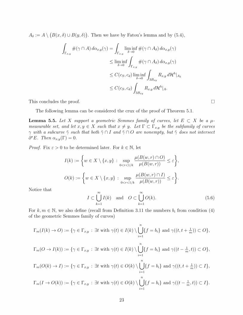
This concludes the proof.
The following lemma can be considered the crux of the proof of Theorem 5.1.
Lemma 5.5. Let X support a geometric Semmes family of curves, let E ⊂ X be a µ-measurable set, and let x, y ∈ X such that x 6= y. Let Γ ⊂ Γx,y be the subfamily of curvesγ with a subcurve γ such that both γ ∩ I and γ ∩ O are nonempty, but γ does not intersect∂∗E. Then αx,y(Γ) = 0.
Proof. Fix ε > 0 to be determined later. For k ∈ N, let
I(k) :=
w ∈ X \ x, y : sup
0<r<1/k
µ(B(w, r) ∩O)
µ(B(w, r))≤ ε
,
O(k) :=
w ∈ X \ x, y : sup
0<r<1/k
µ(B(w, r) ∩ I)
µ(B(w, r))≤ ε
.
Notice that
I ⊂∞⋃k=1
I(k) and O ⊂∞⋃k=1
O(k). (5.6)
For k,m ∈ N, we also define (recall from Definition 3.11 the numbers bi from condition (4)of the geometric Semmes family of curves)
Γm(I(k)→ O) := γ ∈ Γx,y : ∃t with γ(t) ∈ I(k) \n⋃i=1
f = bi and γ((t, t+ 1m
)) ⊂ O,
Γm(O → I(k)) := γ ∈ Γx,y : ∃t with γ(t) ∈ I(k) \n⋃i=1
f = bi and γ((t− 1m, t)) ⊂ O,
Γm(O(k)→ I) := γ ∈ Γx,y : ∃t with γ(t) ∈ O(k) \n⋃i=1
f = bi and γ((t, t+ 1m
)) ⊂ I,
Γm(I → O(k)) := γ ∈ Γx,y : ∃t with γ(t) ∈ O(k) \n⋃i=1
f = bi and γ((t− 1m, t)) ⊂ I.
23

We wish to establish that the αx,y-measure of all of these curve families is zero. For k,m ∈ Nfixed, we will show that αx,y(Γm(I(k) → O)) = 0. Analogous arguments hold for the otherterms.
Let δ < w/(md(x, y)), where w is the “growth speed” from condition (3) of the geometricSemmes family of curves. Next, we take the collection of numbers Aδ and the correspondingsets Aj, j ∈ Z, guaranteed by Definition 3.11.
For j ∈ Z, let Γ(j) denote the collection of curves γ ∈ Γm(I(k) → O) such that thereexists tγ with the property that
γ(tγ) ∈ I(k) ∩ Aj and γ((tγ, tγ + 1/m)) ⊂ O. (5.7)
SinceΓm(I(k)→ O) =
⋃j∈Z
Γ(j),
it suffices to show that αx,y(Γ(j)) = 0 for each j ∈ N.For j ∈ N fixed, equip the space Γx,y with the metric
dj(γ1, γ2) := dH(γ1 ∩ Aj, γ2 ∩ Aj),where γ1, γ2 are any curves in Γx,y and dH is the Hausdorff distance. Now, for γ0 ∈ Γx,y, let
D(γ0, r) := γ ∈ Γx,y : dj(γ, γ0) < r.The set D(γ0, r) is thus a ball in the metric space Γx,y. Due to the conditions satisfied bythe geometric Semmes family of curves, we can now show that αx,y is doubling with respectto the metric dj for small enough balls. More precisely, let us require
r < min
dist(x, y, Aj)
9,cSd(x, y)(aj − aj)
6
. (5.8)
Recall that aj ≤ f < aj in the set Aj. It is easy to verify that the function f is 3/d(x, y)-Lipschitz continuous. Take any γ ∈ Γx,y. We can, by continuity, pick t such that f(γ(t)) =(aj + aj)/2, and then
B
(γ(t),
d(x, y)(aj − aj)6
)⊂ Aj. (5.9)
The curves that intersect B(γ(t), 2r) travel at least the length r inside the ball B(γ(t), 3r).Thus
αx,y(D(γ, 2r)) ≤ αx,y(Γ(B(γ(t), 2r)))
≤∫
Γ(B(γ(t),2r))
1
r
∫γ
χB(γ(t),3r) ds dαx,y(γ)
≤∫
Γx,y
1
r
∫γ
χB(γ(t),3r) ds dαx,y(γ)
≤ cSr
∫B(γ(t),3r)
Rx,y dµ
≤ C(cS, cd)
r
∫B(γ(t),c−2
S r)
Rx,y dµ
≤ C(cS, cd)αx,y(Γ(B(γ(t), c−1S r)))
≤ C(cS, cd)αx,y(D(γ, r)).
(5.10)
24

In the fourth inequality we used the definition of Semmes family of curves, and in the fifthinequality we used the fact that for small enough radii the measure dν := Rx,y dµ is doublingat γ(t), with doubling constant c4
d. In the last two inequalities we used conditions (1) and (2)of the geometric Semmes family of curves. Note that in order to use condition (2) to obtainthe last inequality, we need B(γ(t), c−1
S r) ⊂ Aj, which is guaranteed by (5.8) and (5.9).Now fix γ0 ∈ Γ(j). Let
r < min
w
100c2S
dist(x, y, Aj),w(aj − aj)d(x, y)
100cS,w
10k,
1
m
, (5.11)
and further letD∗(γ0, r) := D(γ0, r) ∩ Γ(j).
Let γ1 ∈ D∗(γ0, r) be such that there is a choice of tγ1 satisfying the condition that for allγ ∈ D∗(γ0, r),
f(γ1(tγ1)) + r/d(x, y) > f(γ(tγ)); (5.12)
recall the definition of “tγ” from (5.7). This condition implies that of all the curves γ ∈D∗(γ0, r), γ1 has the “bad point” γ1(tγ1) almost the furthest away from the inner boundaryof the “annulus” Aj.
Next we show that for all γ ∈ D∗(γ0, r), by the choice of γ1 and by the fact that γ((tγ, tγ+1/m)) ⊂ O, we have
`(γ ∩O ∩B(γ1(tγ1), 10r/w)) ≥ r. (5.13)
This is seen as follows. By the condition γ ∈ D∗(γ0, r) we know that for some t we haveγ(t) ∈ Aj and d(γ(t), γ1(tγ1)) < 2r. If γ has its “bad point” γ(tγ) “earlier” on the curve, i.e.tγ ≤ t, then condition (5.13) is easily satisfied. Let us assume that tγ > t instead. Since fis a 3/d(x, y)-Lipschitz function, we have
f(γ(t)) > f(γ1(tγ1))− 6r/d(x, y). (5.14)
Hence we know that tγ − t < 7r/w, for otherwise the growth condition (3) of the geometricSemmes family of curves and (5.14) would imply that f(γ(tγ)) is too big, violating (5.12).Now we have of course d(γ(tγ), γ(t)) < 7r/w, further implying that d(γ(tγ), γ1(tγ1)) < 9r/w.Thus γ travels at least the length r in O ∩B(γ1(tγ1), 10r/w), since we had r < 1/m. This iscondition (5.13).
Now we can use the definition of the (ordinary) Semmes family of curves to calculate
αx,y(D∗(γ0, r)) ≤1
r
∫D∗(γ0,r)
∫γ
χO∩B(γ1(tγ1 ),10r/w) ds dαx,y(γ)
≤ 1
r
∫Γx,y
∫γ
χO∩B(γ1(tγ1 ),10r/w) ds dαx,y(γ)
≤ cSr
∫O∩B(γ1(tγ1 ),10r/w)
Rx,y dµ
≤ cSc3dε
r
∫B(γ1(tγ1 ),10r/w)
Rx,y dµ.
(5.15)
25

In the last inequality, we used the fact that by the doubling property of µ and by (5.11), Rx,y
is approximately constant in the ball B = B(γ1(tγ1), 10r/w) — more precisely supB Rx,y ≤c3d infB Rx,y — and so, since γ1(tγ1) ∈ I(k),∫
O∩B(γ1(tγ1 ),10r/w)Rx,y dµ∫
B(γ1(tγ1 ),10r/w)Rx,y dµ
≤ c3d
µ(O ∩B(γ1(tγ1), 10r/w))
µ(B(γ1(tγ1), 10r/w))≤ c3
dε.
Now pick t such that γ0(t) ∈ Aj and d(γ0(t), γ1(tγ1)) < r. Then pick another number tsuch that
aj +10cSr
w
3
d(x, y)≤ f(γ0(t)) ≤ aj −
10cSr
w
3
d(x, y). (5.16)
By the 3/d(x, y)-Lipschitz-continuity of the function f we have B(γ0(t), 10cSr/w) ⊂ Aj. Bythe growth condition (3) of the geometric Semmes family of curves and condition (5.16), wecan pick the number t so that it satisfies
w
d(x, y)|t− t| ≤ 10cSr
w
3
d(x, y),
and consequently d(γ0(t), γ0(t)) ≤ 30cSr/w2. Thus we have d(γ0(t), γ1(tγ1)) ≤ 31cSr/w
2.This implies that µ(B(γ1(tγ1), 10r/w)) and µ(B(γ0(t), 10r/w)) are comparable by a factorC = C(cd, cS, w) [BjBj, Lemma 3.6].
Additionally, recall from Section 3.2 that Rx,y is, up to a factor C(cd, λ), constant on theset Aj, and even in a 10r/w-neighborhood of it. This enables us to switch to a different ballin (5.15):
αx,y(D∗(γ0, r)) ≤C(cS, cd, w, λ)ε
r
∫B(γ0(t),10r/w)
Rx,y dµ.
On the other hand, by condition (1) of the geometric Semmes family of curves,
αx,y(Γ(B(γ0(t), 10cSr/w))) ≥ 1
cS
1
10cSr/w
∫B(γ0(t),10r/w)
Rx,y dµ.
Furthermore, by condition (2) and the fact that B(γ0(t), 10cSr/w) ⊂ Aj, we have
Γ(B(γ0(t), 10cSr/w)) ⊂ D(γ0, 10c2Sr/w).
It follows thatαx,y(D∗(γ0, r)) ≤ C(cS, cd, λ, w)εαx,y(D(γ0, 10c2
Sr/w)).
By the doubling property (5.10) of αx,y with respect to the metric dj, where again we needr to be small enough, we now have
αx,y(D∗(γ0, r)) ≤ C(cS, cd, λ, w)εαx,y(D(γ0, r)).
Thus taking ε small enough so that Cε < 23, we get
αx,y(D∗(γ0, r)) ≤ 23αx,y(D(γ0, r)).
26

We recall that D(γ, r) denotes a ball with respect to the metric dj. Now the density of Γ(j)at γ0 is
lim supr→0+
αx,y(D(γ0, r) ∩ Γ(j))
αx,y(D(γ0, r))= lim sup
r→0+
αx,y(D∗(γ0, r))
αx,y(D(γ0, r))≤ 2/3 < 1.
Furthermore, γ0 ∈ Γ(j) was arbitrary. On the other hand, for a Borel regular outer measurethat is doubling for sufficiently small radii, such as αx,y, we know that Lebesgue’s differenti-ation theorem holds, see e.g. [Hei, Theorem 1.8]. In particular, almost every point of a sethas density 1, so now we must have αx,y(Γ(j)) = 0. This is the desired result.
For the remainder of the proof, fix a curve
γ ∈ Γx,y \⋃
k,m∈N
(Γm(I(k)→ O)∪Γm(O → I(k))∪Γm(O(k)→ I)∪Γm(I → O(k))
); (5.17)
by the above result, this holds for αx,y-a.e. curve. We wish to show that γ ∈ Γx,y \ Γ.First let us assume that γ(u) ∈ I and γ(v) ∈ O for some 0 ≤ u < v ≤ `γ so that thereis no bi (defined in condition (4) of the geometric Semmes family of curves) in the interval(f(γ(u)), f(γ(v))).
We note that the sets I(k) and O(k) are closed, which can be seen as follows. Letzi ∈ I(k), i = 1, 2, . . ., and zi → z. Now, for any given r < 1/k we simply calculate
µ(B(z, r) ∩O)
µ(B(z, r))= lim
i→∞
µ(B(zi, r − d(zi, z)) ∩O)
µ(B(zi, r − d(zi, z)))≤ ε,
which gives the result. Now we recall (5.6), and note that I(k)∞k=1 and O(k)∞k=1 areincreasing sequences of closed sets. Thus there exists some k0 ∈ N such that γ(u) ∈ I(k0)and γ(v) ∈ O(k0). We define
u0 := supt ∈ [u, v) : γ(t) ∈ I(k0),
and note that I(k0) is closed and I(k0) ∩O(k0) = ∅, as we can choose ε < 12. Thus we have
γ(u0) ∈ I(k0) and u0 < v. Next define
v0 := inft ∈ (u0, v] : γ(t) ∈ O(k0).
By the same reasoning as above, we can conclude that γ(v0) ∈ O(k0), and u ≤ u0 < v0 ≤ v.Clearly we also have
γ(t) /∈ I(k0) ∪O(k0) for t ∈ (u0, v0).
Now, by (5.17) we know that there exist u0 < u1 < v1 < v0 such that γ(u1) ∈ I andγ(v1) ∈ O. By the same reasoning as above, we find k1 > k0 and u0 < u1 < v1 < v0 suchthat γ(u1) ∈ I(k1), γ(v1) ∈ O(k1), and
γ(t) /∈ I(k1) ∪O(k1) for t ∈ (u1, v1).
Continuing like this, we get a sequence ki →∞ and sequences ui, vi such thatu0 < u1 < u2 < . . . , v0 > v1 > . . . ,ui < vi,γ(ui) ∈ I(ki), γ(vi) ∈ O(ki),γ(t) /∈ I(ki) ∪O(ki) for t ∈ (ui, vi), for all i ∈ N.
27
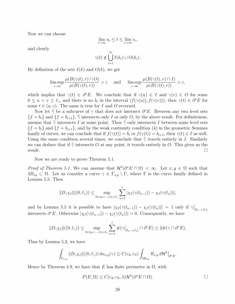
Now we can chooselimi→∞
ui ≤ t ≤ limi→∞
vi,
and clearly
γ(t) /∈∞⋃i=1
I(ki) ∪O(ki).
By definition of the sets I(k) and O(k), we get
lim supr→0
µ(B(γ(t), r) ∩O)
µ(B(γ(t), r))> ε and lim sup
r→0
µ(B(γ(t), r) ∩ I)
µ(B(γ(t), r))> ε,
which implies that γ(t) ∈ ∂∗E. We conclude that if γ(u) ∈ I and γ(v) ∈ O for some0 ≤ u < v ≤ `γ, and there is no bi in the interval (f(γ(u)), f(γ(v))), then γ(t) ∈ ∂∗E forsome t ∈ (u, v). The same is true for I and O reversed.
Now let γ be a subcurve of γ that does not intersect ∂∗E. Between any two level setsf = bi and f = bi+1, γ intersects only I or only O, by the above result. For definiteness,assume that γ intersects I at some point. Then γ only intersects I between some level setsf = bi and f = bi+1, and by the weak continuity condition (4) in the geometric Semmesfamily of curves, we can conclude that if f(γ(t)) = bi or f(γ(t)) = bi+1, then γ(t) ∈ I as well.Using the same condition several times, we conclude that γ travels entirely in I. Similarlywe can deduce that if γ intersects O at any point, it travels entirely in O. This gives us theresult.
Now we are ready to prove Theorem 5.1.
Proof of Theorem 5.1. We can assume that Hh(∂∗E ∩ Ω) < ∞. Let x, y ∈ Ω such that3Bxy ⊂ Ω. Let us consider a curve γ ∈ Γx,y \ Γ, where Γ is the curve family defined inLemma 5.5. Then
‖DγχI‖((0, `γ)) ≤ sup0<t0<...<tl<`γ
l∑n=1
|χI(γ(tn−1))− χI(γ(tn))|,
and by Lemma 5.5 it is possible to have |χI(γ(tn−1)) − χI(γ(tn))| = 1 only if γ∣∣[tn−1,tn]
intersects ∂∗E. Otherwise |χI(γ(tn−1))− χI(γ(tn))| = 0. Consequently, we have
‖DγχI‖((0, `γ)) ≤ sup0<t0<...<tl<`γ
l∑n=1
#(γ∣∣[tn−1,tn]
∩ ∂∗E) ≤ 2#(γ ∩ ∂∗E).
Thus by Lemma 5.2, we have∫Γx,y
‖DγχI‖((0, `γ)) dαx,y(γ) ≤ C(cd, cS)
∫3Bxy
Rx,y dHh∣∣∂∗E
.
Hence by Theorem 4.9, we have that E has finite perimeter in Ω, with
P (E,Ω) ≤ C(cd, cS, λ)Hh(∂∗E ∩ Ω).
28

Remark 5.18. By combining Theorem 5.1 with the discussion in the beginning of thissection, we conclude that always Hh(∂∗E ∩ Ω) ≈ P (E,Ω), with constants of comparisonC = C(cd, cP , τ). In particular, from the relative isoperimetric inequality (2.11) we get thefollowing strong relative isoperimetric inequality as promised in [KKST]:
minµ(B ∩ E), µ(B \ E) ≤ C rad(B)Hh(∂∗E ∩ λB)
for any µ-measurable E ⊂ X and any ball B.
6 Examples of spaces supporting a geometric Semmes
family of curves
The geometric version of the Semmes family of curves proposed in this article would not becompelling if we could not show that the classical metric space, the Euclidean space equippedwith the Lebesgue measure, supports such a geometric family. In this section we will showthat the Euclidean space as well as certain examples of non-Euclidean spaces support thegeometric Semmes family of curves.
It was pointed out to us by Riikka Kangaslampi that the boundaries of certain hyperbolicbuildings, constructed by Bourdon and Pajot in [BoPaj], are unlikely to support such ageometric version of a Semmes family of curves (although they do support the standardSemmes family of curves and hence the (1, 1)-Poincare inequality) because geodesics betweentwo distinct points in these spaces cross each other at all scales.
Example 6.1 (Euclidean spaces). In the Euclidean space Rn a geometric Semmes familyof curves is simple to construct. For any points x, y, consider the hyperplane orthogonal tothe line segment [x, y], and lying at an equal distance from both points. Take an (n − 1)-dimensional disk Bn−1 in the hyperplane, centered at the intersection point and with radius|x − y|/2. For any z ∈ Bn−1, let γz be the curve consisting of two line segments: [x, z] and[z, y]. Let Γx,y := γz : z ∈ Bn−1. Due to the shape of this type of curve family, it is oftencalled a Semmes pencil of curves.
We define the measure αx,y as follows: if Γ ⊂ Γx,y,
αx,y(Γ) := Hn−1(z ∈ Bn−1 : γz ∈ Γ)/Hn−1(Bn−1).
The “annuli” Aj can be defined as in (3.9). Now all the conditions are easy to verify — forexample, for a Borel set A ⊂ Rn, the αx,y-measurability of Γx,y 3 γ 7→ `(γ ∩A) follows as inthe classical coarea formula, see e.g. [AFP, Lemma 2.99]. The αx,y-measurability of Γx,y 3γ 7→ #(γ∩A) can be deduced from the same lemma. Perhaps the most non-trivial conditionto check is that of the (ordinary) Semmes family of curves. For example, if A consists of pointsthat are closer to x than to y, we can define Aj := A∩ [B(x, 2−jd(x, y))\B(x, 2−j−1d(x, y))],
29
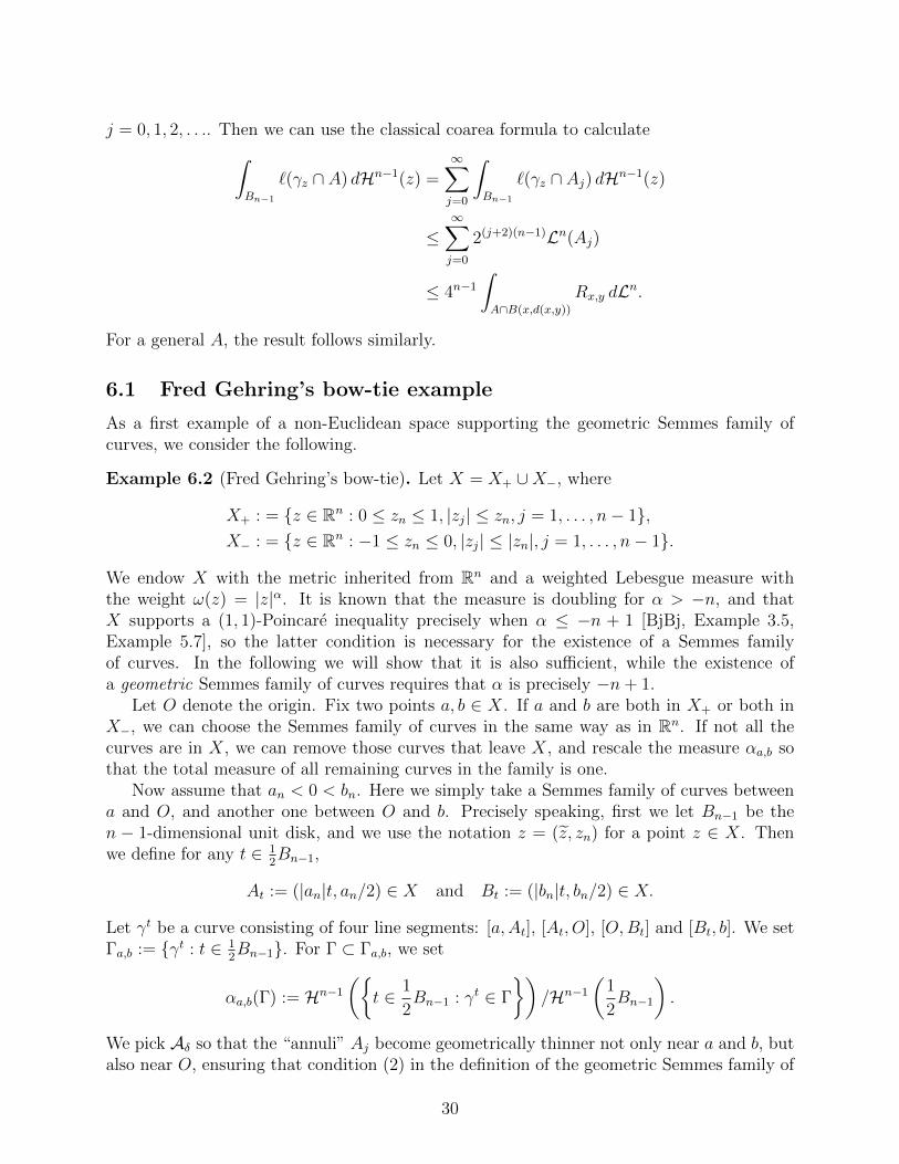
j = 0, 1, 2, . . .. Then we can use the classical coarea formula to calculate∫Bn−1
`(γz ∩ A) dHn−1(z) =∞∑j=0
∫Bn−1
`(γz ∩ Aj) dHn−1(z)
≤∞∑j=0
2(j+2)(n−1)Ln(Aj)
≤ 4n−1
∫A∩B(x,d(x,y))
Rx,y dLn.
For a general A, the result follows similarly.
6.1 Fred Gehring’s bow-tie example
As a first example of a non-Euclidean space supporting the geometric Semmes family ofcurves, we consider the following.
Example 6.2 (Fred Gehring’s bow-tie). Let X = X+ ∪X−, where
X+ : = z ∈ Rn : 0 ≤ zn ≤ 1, |zj| ≤ zn, j = 1, . . . , n− 1,X− : = z ∈ Rn : −1 ≤ zn ≤ 0, |zj| ≤ |zn|, j = 1, . . . , n− 1.
We endow X with the metric inherited from Rn and a weighted Lebesgue measure withthe weight ω(z) = |z|α. It is known that the measure is doubling for α > −n, and thatX supports a (1, 1)-Poincare inequality precisely when α ≤ −n + 1 [BjBj, Example 3.5,Example 5.7], so the latter condition is necessary for the existence of a Semmes familyof curves. In the following we will show that it is also sufficient, while the existence ofa geometric Semmes family of curves requires that α is precisely −n+ 1.
Let O denote the origin. Fix two points a, b ∈ X. If a and b are both in X+ or both inX−, we can choose the Semmes family of curves in the same way as in Rn. If not all thecurves are in X, we can remove those curves that leave X, and rescale the measure αa,b sothat the total measure of all remaining curves in the family is one.
Now assume that an < 0 < bn. Here we simply take a Semmes family of curves betweena and O, and another one between O and b. Precisely speaking, first we let Bn−1 be then − 1-dimensional unit disk, and we use the notation z = (z, zn) for a point z ∈ X. Thenwe define for any t ∈ 1
2Bn−1,
At := (|an|t, an/2) ∈ X and Bt := (|bn|t, bn/2) ∈ X.
Let γt be a curve consisting of four line segments: [a,At], [At, O], [O,Bt] and [Bt, b]. We setΓa,b := γt : t ∈ 1
2Bn−1. For Γ ⊂ Γa,b, we set
αa,b(Γ) := Hn−1
(t ∈ 1
2Bn−1 : γt ∈ Γ
)/Hn−1
(1
2Bn−1
).
We pick Aδ so that the “annuli” Aj become geometrically thinner not only near a and b, butalso near O, ensuring that condition (2) in the definition of the geometric Semmes family of
30
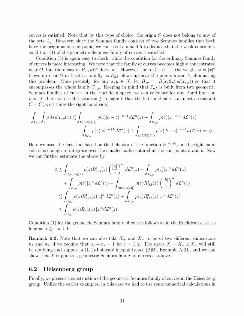
curves is satisfied. Note that by this type of choice, the origin O does not belong to any ofthe sets Aj. However, since the Semmes family consists of two Semmes families that bothhave the origin as an end point, we can use Lemma 4.5 to deduce that the weak continuitycondition (4) of the geometric Semmes family of curves is satisfied.
Condition (3) is again easy to check, while the condition for the ordinary Semmes familyof curves is more interesting. We note that the family of curves becomes highly concentratednear O, but the measure Ra,b dLn does not. However, for α ≤ −n + 1 the weight ω = |x|αblows up near O at least as rapidly as Ra,b blows up near the points a and b, eliminatingthis problem. More precisely, for any x, y ∈ X, let Bxy := B(x, 2
√nd(x, y)) so that it
encompasses the whole family Γx,y. Keeping in mind that Γa,b is built from two geometricSemmes families of curves in the Euclidean space, we can calculate for any Borel functionρ on X (here we use the notation . to signify that the left-hand side is at most a constantC = C(n, α) times the right-hand side)∫
Γa,b
∫γ
ρ ds dαa,b(γ) .∫B(a,3|a|/4)
ρ(z)|a− z|−n+1 dLn(z) +
∫BaO
ρ(z)|z|−n+1 dLn(z)
+
∫BOb
ρ(z)|z|−n+1 dLn(z) +
∫B(b,3|b|/4|)
ρ(z)|b− z|−n+1 dLn(z) =: ♦.
Here we used the fact that based on the behavior of the function |z|−n+1, on the right-handside it is enough to integrate over the smaller balls centered at the end points a and b. Nowwe can further estimate the above by
♦ ≤∫B(a,3|a|/4)
ρ(z)R1a,O(z)
(|a|4
)αdLn(z) +
∫BaO
ρ(z)|z|α dLn(z)
+
∫BOb
ρ(z)|z|α dLn(z) +
∫B(b,3|b|/4|)
ρ(z)R2O,b(z)
(|b|4
)αdLn(z)
.∫BaO
ρ(z)R1a,O(z)|z|α dLn(z) +
∫BOb
ρ(z)R2O,b(z)|z|α dLn(z)
≤∫Bab
ρ(z)Ra,b(z) |z|αdLn(z).
Condition (1) for the geometric Semmes family of curves follows as in the Euclidean case, aslong as α ≥ −n+ 1.
Remark 6.3. Note that we can also take X+ and X− to be of two different dimensionsn1 and n2, if we require that αi + ni = 1 for i = 1, 2. The space X = X+ ∪ X− will stillbe doubling and support a (1, 1)-Poincare inequality, see [BjBj, Example A.24], and we canshow that X supports a geometric Semmes family of curves as above.
6.2 Heisenberg group
Finally, we present a construction of the geometric Semmes family of curves in the Heisenberggroup. Unlike the earlier examples, in this case we had to use some numerical calculations in
31
the verification of the conditions. Let us model the Heisenberg group as H = (R3, ∗), wherethe multiplication of p, q ∈ H is given by
(p1, p2, p3) ∗ (q1, q2, q3) =(p1 + q1, p2 + q2, p3 + q3 + 1
2(p1q2 − p2q1)
).
The group law respects the dilations δr(p1, p2, p3) := (rp1, rp2, r2p3), r > 0. We have the
following left-invariant vector fields in H:
Xp = ∂p1 − p22∂p3 ,
Yp = ∂p2 + p12∂p3 ,
Zp = ∂p3 ,
which satisfy [X, Y ] = Z. At each point p ∈ H, the horizontal space HpH ⊂ TpH is spannedby Xp and Yp. For an interval I ⊂ R, a piecewise C1 curve p : I → H is horizontal ifp(t) ∈ Hp(t)H whenever it exists.
We endow H with a sub-Riemannian metric, defined on the horizontal spaces, so that Xand Y are everywhere orthonormal. Let ‖ · ‖ be the norm induced by this inner product.Let γ : I → H be a horizontal curve. We define the length of γ by
`(γ) :=
∫I
‖γ(t)‖ dt.
The Carnot-Caratheodory distance between two points p, q ∈ H is
dc(p, q) := min`(γ) : γ is horizontal and connects p and q
The Carnot-Caratheodory metric is bi-Lipschitz equivalent to the metric d(p, q) := ‖p−1∗q‖H,where ‖p‖H := (p4
1 + p42 + p2
3)1/4.Next, we construct a geometric Semmes family of curves in the Heisenberg group.
Remark 6.4. As we have seen previously, in Rn the natural way to construct a (geometric)Semmes family of curves is to choose some hypersurface S between the points x and y, andthen to connect the points of S by geodesics to x and y. However, in the Heisenberg group,this construction does not work. This can be seen by considering geodesics starting fromthe origin, presented in (6.5) (parametrized by arc-length). The z3-component is z3(t) =a12t3 + O(t5). The condition (3.4) can hold only if the curves cover approximately the same
portion of each sphere around x (in this case the origin), but this would require that z3(t)decrease at the rate t2 as t→ 0.
We will first construct a family of curves Γ0 starting from the origin. We will then use thiscurve family to construct the geometric Semmes family. Let S := s ∈ H : dc(s, δ2(s)) = 1.For s ∈ S, let γs be a geodesic joining the points s and δ2(s), and let
γs :=⋃k∈Z
δ2k(γs).
The family Γ0 will consist of the curves γs, s ∈ S, that are not “too vertical” — we willspecify this later. This construction forces the curves to stay far enough from each other as
32

they get close to the origin, as described in Remark 6.4. The distance between two curvesat the end of one geodesic subcurve δ2k(γs) is exactly half of the distance at the other end,and therefore the distance is well under control at the end points of each geodesic subcurve.Next we will consider the behavior of the distance between the end points.
Geodesics γ(t) = (z1(t), z2(t), z3(t)) that start from the origin at unit speed can beexpressed as
z1(t) =cos θ sin(at)− sin θ(1− cos(at))
a,
z2(t) =sin θ sin(at) + cos θ(1− cos(at))
a,
z3(t) =at− sin(at)
2a2,
(6.5)
where |a| ≤ 2π, 0 ≤ θ < 2π and t ∈ [0, 1], see for example [BelRis]. The initial velocity of acurve is X cos θ + Y sin θ.
We want to construct the geodesic γs, s ∈ S, with length 1 and connecting the pointss = (s1, s2, s3) and δ2(s) = (2s1, 2s2, 4s3). If we left-translate the geodesic γs so that it startsfrom the origin, then the endpoint is (s1, s2, s3)−1 ∗ (2s1, 2s2, 4s3) = (s1, s2, 3s3). Thus wehave s1 = z1(1), s2 = z2(1) and s3 = 1
3z3(1), and the geodesic is
γs(t) =(z1(1), z2(1), 1
3z3(1)
)∗ (z1(t), z2(t), z3(t))
=
(cos θ(sin a+ sin(at))− sin θ(2− cos a− cos(at))
a,
sin θ(sin a+ sin(at)) + cos θ(2− cos a− cos(at))
a,
a+ 3at+ 2 sin a− 6 sin(at)− 3 sin(a− at)6a2
), t ∈ (0, 1).
(6.6)
We choose Γ0 to consist of all geodesics γs such that |a| ≤ 1.Now we are ready to construct the geometric Semmes family of curves. We associate to
each point x ∈ H the left-translated curve family Γx = x ∗ γ : γ ∈ Γ0. For x, y ∈ H, letBxy := B(x, 100dc(x, y)) and let M := m ∈ Bxy : dc(m,x) = dc(m, y).
If a point m ∈ M can be connected to x by a subcurve of a curve in Γx and to y by asubcurve of a curve in Γy, then we will call the union of these two curves γm. The Semmesfamily of curves Γx,y connecting x and y consists of all such curves. We endow the curvefamily with the measure
αxy(Γ) =H3(Γ ∩M)
H3(Γx,y ∩M),
where H3 denotes the 3-dimensional Hausdorff measure.If x−1 ∗ y is close to horizontal, it is easy to see that there are plenty of curves in Γx,y.
The “worst” situation occurs when x−1 ∗ y = (0, 0, t) for some t ∈ R, as the shortest possiblecurves connecting x and y are not included in the curve family Γx,y, since we require that|a| ≤ 1. Therefore we had to choose the reference set Bxy to be large enough so that thecurve family is not empty even in this case. The main difficulty in verifying that this family
33

of curves satisfies the conditions of the geometric Semmes family of curves is in confirmingthat condition (2) is satisfied. More precisely, we need to show that the distance betweentwo geodesic subcurves γs remains comparable to the distance of the end points. This wasdone by numerical computations with the help of Mathematica when |a| ≤ 1, using (6.6).
Remark 6.7. Instead of the set S, we could use for example the unit sphere to constructthe curves. One should get an equally well behaving family of curves this way, but our choiceof S makes it easier to find an explicit representation for the curves and thus to check thatthe distance between two curves behaves well.
References
[AK] D. Aalto and J. Kinnunen. The discrete maximal operator in metric spaces, J.Anal. Math. 111 (2010) 369–390.
[Am1] L. Ambrosio. Some fine properties of sets of finite perimeter in Ahlfors regularmetric measure spaces, Adv. Math. 159 (2001) 51–67.
[Am2] L. Ambrosio. Fine properties of sets of finite perimeter in doubling metric measurespaces, Set-Valued Anal. 10 (2002) 111–128.
[AmDi] L. Ambrosio and S. Di Marino. Equivalent definitions of BV space and of total vari-ation on metric measure spaces, Manuscript, http://cvgmt.sns.it/paper/1860/(2012) 1–36.
[AFP] L. Ambrosio, N. Fusco, and D. Pallara. Functions of bounded variation and freediscontinuity problems, Oxford Mathematical Monographs. The Clarendon Press,Oxford University Press, New York, 2000. xviii+434 pp.
[AMP] L. Ambrosio, M. Miranda, Jr., and D. Pallara. Special functions of bounded vari-ation in doubling metric measure spaces, Calculus of variations: topics from themathematical heritage of E. De Giorgi, 1–45, Quad. Mat., 14, Dept. Math., Sec-onda Univ. Napoli, Caserta, 2004.
[AT] L. Ambrosio and P. Tilli. Topics on analysis in metric spaces, Oxford LectureSeries in Mathematics and its Applications, 25. Oxford University Press, Oxford,2004. viii+133 pp.
[BelRis] A. Bellaıche and J.-J. Risler. Sub-Riemannian geometry, Progress in Mathematics144 Birkhauser Verlag, Basel (1996) viii+393 pp.
[BjBj] A. Bjorn and J. Bjorn. Nonlinear potential theory on metric spaces, EMS Tracts inMathematics, 17. European Mathematical Society (EMS), Zurich, 2011. xii+403pp.
[BoPaj] M. Bourdon and H. Pajot. Poincare inequalities and quasiconformal structure onthe boundary of some hyperbolic buildings, Proc. Amer. Math. Soc. 127 (1999)2315–2324.
34
[Buc] S. Buckley. Is the maximal function of a Lipschitz function continuous?, Ann.Acad. Sci. Fenn. Math. 24 (1999) 519–528.
[EvGa] L. C. Evans and R. Gariepy. Measure theory and fine properties of functions, Stud-ies in Advanced Mathematics, CRC press, Boca Raton, FL, 1992. viii+268 pp.
[Fed] H. Federer. Geometric measure theory, Die Grundlehren der mathematischen Wis-senschaften 153 (1969), Springer New York xiv+676 pp.
[Fug] B. Fuglede. Extremal length and functional completion, Acta Math. 98 (1957) 171–219.
[Haj] P. Haj lasz. Sobolev spaces on metric-measure spaces, Contemporary Mathematics338 (2003) 173–218.
[HajKo] P. Haj lasz and P. Koskela. Sobolev met Poincare, Mem. Amer. Math. Soc. 145(2000) no. 688, x+101 pp.
[HKT] T. Heikkinen, P. Koskela, and H. Tuominen. Sobolev type spaces from generalizedPoincare inequalities, Studia Math. 181 (2007) 1–16.
[Hei] J. Heinonen. Lectures on analysis on metric spaces, Universitext. Springer-Verlag,New York (2001) x+140 pp.
[HKST] J. Heinonen, P. Koskela, N. Shanmugalingam, and J. Tyson. Sobolev classes ofBanach space-valued functions and quasiconformal mappings, J. Anal. Math. 85(2001) 87–139.
[KKST] J. Kinnunen, R. Korte, N. Shanmugalingam, and H. Tuominen. A characterizationof Newtonian functions with zero boundary values, Calc. Var. Partial DifferentialEquations 43 (2012) no. 3-4, 507–528.
[KL] R. Korte and P. Lahti. Relative isoperimetric inequalities and sufficient conditionsfor finite perimeter on metric spaces, to appear in Ann. Inst. H. Poincare Anal.Non Lineaire.
[KST] P. Koskela, N. Shanmugalingam, and H. Tuominen. Removable sets for thePoincare inequality on metric spaces, Indiana Univ. Math. J. 49 (2000) 333–352.
[LT] P. Lahti and H. Tuominen. A pointwise characterization of functions of boundedvariation on metric spaces, to appear in Ric. Mat.
[Mir] M. Miranda Jr. Functions of bounded variation on “good” metric spaces, J. Math.Pures Appl. (9) 82 (2003) 975–1004.
[Oht] M. Ohtsuka. Extremal length and precise functions, GAKUTO International Series.Mathematical Sciences and Applications 19 (2003), Gakkotosho Co. Ltd. Tokyovi+343 pp.
35
[Roy] H. L. Royden. Real analysis, Macmillan Publishing Company, New York (3rd Edi-tion) (1988) xx+444 pp.
[Rud] W. Rudin. Real and complex analysis, McGraw-Hill Book Co., New York (3rdEdition) (1987) xiv+416 pp.
[Sem] S. Semmes. Finding curves on general spaces through quantitative topology, withapplications to Sobolev and Poincare inequalities, Selecta Math. (N.S.) 2 (1996)155–296.
[Shan] N. Shanmugalingam. Newtonian spaces: an extension of Sobolev spaces to metricmeasure spaces, Rev. Mat. Iberoamericana 16 (2000) no. 2, 243–279.
[Vai] J. Vaisala. Lectures on n-dimensional quasiconformal mappings, Lecture Notes inMathematics 229 (1971), Springer-Verlag, Berlin-New York xiv+144 pp.
[Zie] W. P. Ziemer. Weakly differentiable functions, Graduate Texts in Mathematics120 (1989), Springer New York xvi+308 pp.
Address:
R.K.: Department of Mathematics and Statistics, P.O. Box 68, FI-00014 University ofHelsinki, Finland.E-mail: [email protected]
P.L.: Department of Mathematics, P.O. Box 11100, FI-00076 Aalto University, Finland.E-mail: [email protected]
N.S.: Department of Mathematical Sciences, P.O. Box 210025, University of Cincinnati,Cincinnati, OH 45221–0025, U.S.A.E-mail: [email protected]
36