sensor models - university of arizonadial/ece531/sensor_models.pdf2 sensor models 3 fall 2005...
TRANSCRIPT

1
ECE/OPTI 531 – Image Processing Lab for Remote Sensing Fall 2005
Sensor Models
Reading: Chapter 3
Fall 2005Sensor Models 2
Sensor Models
• LSI System Model• Spatial Response• Spectral Response• Signal Amplification, Sampling, and
Quantization• Simplified Sensor Model• Geometric Distortion
2
Fall 2005Sensor Models 3
Overall Sensor Model
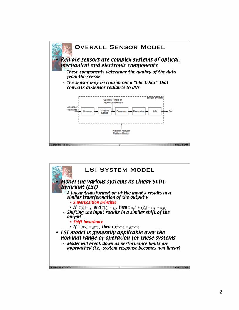
• Remote sensors are complex systems of optical,mechanical and electronic components– These components determine the quality of the data
from the sensor– The sensor may be considered a “black-box” that
converts at-sensor radiance to DNs
Fall 2005Sensor Models 4
LSI System Model
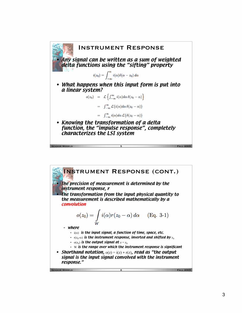
• Model the various systems as Linear Shift-Invariant (LSI)– A linear transformation of the input x results in a
similar transformation of the output y• Superposition principle• If T[f1] = g1 and T[f2] = g2 , then T[a1f1 + a2f2] = a1g1 + a2g2
– Shifting the input results in a similar shift of theoutput
• Shift invariance• If T[f(x)] = g(x) , then T[f(x-x0)] = g(x-x0)
• LSI model is generally applicable over thenominal range of operation for these systems– Model will break down as performance limits are
approached (i.e., system response becomes non-linear)
3
Fall 2005Sensor Models 5
Instrument Response
• Any signal can be written as a sum of weighteddelta functions using the “sifting” property
• What happens when this input form is put intoa linear system?
• Knowing the transformation of a deltafunction, the “impulse response”, completelycharacterizes the LSI system
Fall 2005Sensor Models 6
Instrument Response (cont.)
• The precision of measurement is determined by theinstrument response, r
• The transformation from the input physical quantity tothe measurement is described mathematically by aconvolution
– where• i(α) is the input signal, a function of time, space, etc.• r(z0-α) is the instrument response, inverted and shifted by z0
• o(z0) is the output signal at z = z0
• W is the range over which the instrument response is significant• Shorthand notation, o(z) = i(z) ∗ r(z), read as “the output
signal is the input signal convolved with the instrumentresponse.”

4
Fall 2005Sensor Models 7
Input and Impulse Response
Convolution Operation
Output
1-D Convolution Example
• The measured value at z0 is anaverage of the input signal inthe vicinity of z0, weighted overthe range W by the instrumentresponse
Fall 2005Sensor Models 8
Resolution
• Any instrument that measures a physicalquantity is limited in the amount of detail itcan capture– This limit is referred to as the instrument’s “resolution”– “Resolution” is a term that is widely used, but often
misunderstood• The width W of the instrument response defines
the spatial resolution, or effective GIFOV
5
Fall 2005Sensor Models 9
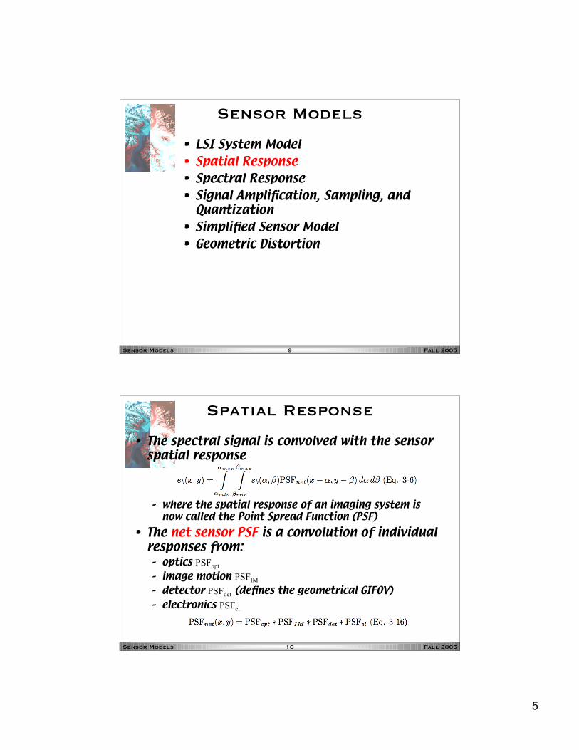
Sensor Models
• LSI System Model• Spatial Response• Spectral Response• Signal Amplification, Sampling, and
Quantization• Simplified Sensor Model• Geometric Distortion
Fall 2005Sensor Models 10
Spatial Response
• The spectral signal is convolved with the sensorspatial response
– where the spatial response of an imaging system isnow called the Point Spread Function (PSF)
• The net sensor PSF is a convolution of individualresponses from:– optics PSFopt
– image motion PSFIM
– detector PSFdet (defines the geometrical GIFOV)– electronics PSFel

6
Fall 2005Sensor Models 11
PSF Properties
• The net sensor PSF is wider than the GIFOVbecause of– PSFopt in both directions– PSFIM
• cross-track for whiskbroom scanners• in-track for pushbroom scanners
– PSFel cross-track for whiskbroom scanners• Reasonable assumption in many cases is that
the PSF is separable in the cross-track and in-track directions
Fall 2005Sensor Models 12
PSF Comparison
0
10
20
30
40
0
10
20
30
40
0
0.2
0.4
0.6
0.8
1
x 10-3
0
10
20
30
40
0
10
20
30
40
-2
0
2
4
6
8
x 10-4
0
10
20
30
40
0
10
20
30
40-1
0
1
2
3
4
5
6
7
x 10-4
0
10
20
30
40
0
10
20
30
40-2
0
2
4
6
8
x 10-4
0
10
20
30
40
0
10
20
30
40
0
0.2
0.4
0.6
0.8
1
normalized detector PSFdet
AVHRR MSS
SPOT HRV TM
cross-trackin-track
significant “out-of-pixel” response in all four systems

7
Fall 2005Sensor Models 13
Sensor Models
• LSI System Model• Spatial Response• Spectral Response• Signal Amplification, Sampling, and
Quantization• Simplified Sensor Model• Geometric Distortion
Fall 2005Sensor Models 14
Spectral Response
• The at-sensor radiance is transferred to thesensor image plane by the camera equation
– where• τo(λ) is the optics spectral transmittance• N is the optics f-number, given by the ratio of the optical
focal length divided by the aperture stop diameter• the optical magnification is assumed to be one
• The spectral responsivity Rb(λ) weights the imageplane irradiance to yield a signal value
8
Fall 2005Sensor Models 15
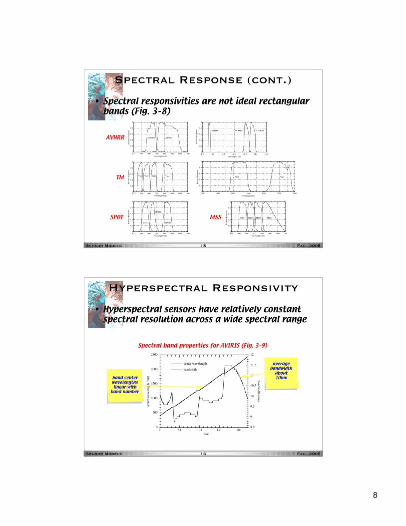
Spectral Response (cont.)
• Spectral responsivities are not ideal rectangularbands (Fig. 3–8)
0
0.2
0.4
0.6
0.8
1
400 500 600 700 800 900 1000 1100
Rel
ativ
e R
esponse
wavelength (nm)
AVHRR1 AVHRR2
0
0.2
0.4
0.6
0.8
1
400 500 600 700 800 900 1000 1100
Rel
ativ
e R
esponse
wavelength (nm)
MSS1 MSS2 MSS3 MSS4
0
0.2
0.4
0.6
0.8
1
400 500 600 700 800 900 1000 1100
Rel
ativ
e R
esponse
wavelength (nm)
TM1 TM2 TM3 TM4
0
0.2
0.4
0.6
0.8
1
400 500 600 700 800 900 1000 1100
Rel
ativ
e R
esponse
wavelength (nm)
SPOT1
SPOT2
SPOT3
0
0.2
0.4
0.6
0.8
1
2.5 4.5 6.5 8.5 10.5 12.5 14.5
Rel
ativ
e R
esponse
wavelength (µm)
AVHRR3 AVHRR4 AVHRR5
0
0.2
0.4
0.6
0.8
1
1200 1400 1600 1800 2000 2200 2400
Rel
ativ
e R
esponse
wavelength (nm)
TM5 TM7
AVHRR
TM
SPOT MSS
Fall 2005Sensor Models 16
Hyperspectral Responsivity
• Hyperspectral sensors have relatively constantspectral resolution across a wide spectral range
band center wavelengths linear with
band number
0
500
1000
1500
2000
2500
8.5
9
9.5
10
10.5
11
11.5
12
1 51 101 151 201
center wavelength
bandwidth
cente
r w
avel
ength
(nm
)ban
dw
idth
(nm
)
band
average bandwidth
about 10nm
Spectral band properties for AVIRIS (Fig. 3–9)
9
Fall 2005Sensor Models 17
Sensor Models
• LSI System Model• Spatial Response• Spectral Response• Signal Amplification, Sampling, and
Quantization• Simplified Sensor Model• Geometric Distortion
Fall 2005Sensor Models 18
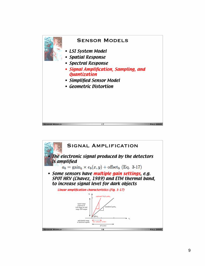
Signal Amplification
• The electronic signal produced by the detectorsis amplified
• Some sensors have multiple gain settings, e.g.SPOT HRV (Chavez, 1989) and ETM thermal band,to increase signal level for dark objects
signal rangerequired at
A/D input for fullrange DN output
ab
eb
anticipated range
optional high gainb
offsetb
all scenes
standard gainb
of detected signals low radiance scenes
Linear amplification characteristics (Fig. 3–17)
10
Fall 2005Sensor Models 19
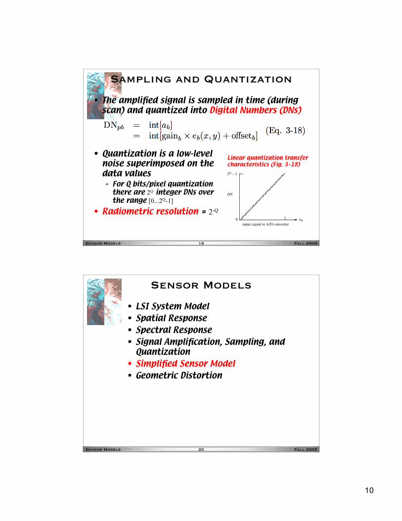
Sampling and Quantization
• The amplified signal is sampled in time (duringscan) and quantized into Digital Numbers (DNs)
DN
0
2Q – 1
input signal to A/D converter
ab
• Quantization is a low-levelnoise superimposed on thedata values– For Q bits/pixel quantization
there are 2Q integer DNs overthe range [0...2Q-1]
• Radiometric resolution = 2-Q
Linear quantization transfercharacteristics (Fig. 3–18)
Fall 2005Sensor Models 20
Sensor Models
• LSI System Model• Spatial Response• Spectral Response• Signal Amplification, Sampling, and
Quantization• Simplified Sensor Model• Geometric Distortion

11
Fall 2005Sensor Models 21
Effective Sensor Model
• Total measured signal at pixel p in band b
– where• DNpb is the Digital Number at pixel p in band b• Lλ(x,y) is the at-sensor spectral radiance from scene
location (x,y)• Kb is a gain coefficient for band b that includes sensor
gain, detector spectral responsivity and spectral filtertransmittance
• offsetb is the sensor offset coefficient for band b• the gain and offset are effective quantities, averaged
over an effective spectral band
Fall 2005Sensor Models 22
Gain-Offset Model
• The three integrals are over:– the effective spectral response range of band b
(spectral resolution)– the effective spatial response range in-track and cross-
track (spatial resolution)• Assume a band- and space-integrated at-sensor
radiance Lpb at pixel p, band b. Then,
– DNs are linearly proportional to the total at-sensorradiance
– Ignores radiometric quantization and nonuniformresponse within spectral bands and the GIFOV
– Simplifies modeling and radiometric calibration of thesensor
12
Fall 2005Sensor Models 23
Sensor Models
• LSI System Model• Spatial Response• Spectral Response• Signal Amplification, Sampling, and
Quantization• Simplified Sensor Model• Geometric Distortion
Fall 2005Sensor Models 24
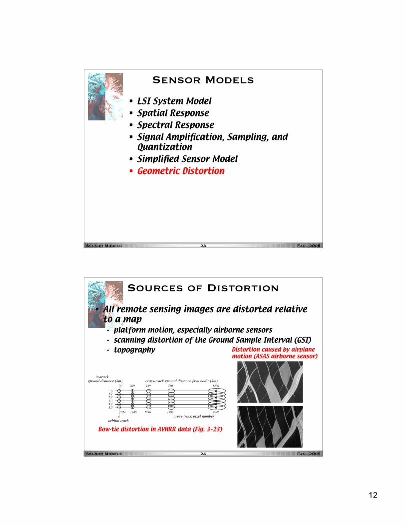
Sources of Distortion
• All remote sensing images are distorted relativeto a map– platform motion, especially airborne sensors– scanning distortion of the Ground Sample Interval (GSI)– topography Distortion caused by airplane
motion (ASAS airborne sensor)
cross-track ground distance from nadir (km)in-track
ground distance (km)
01.12.2
3.34.4
5.5
0 200 430 750 1400
1024 20481280 1536 1792
cross-track pixel numberorbital track
Bow-tie distortion in AVHRR data (Fig. 3–23)

13
Fall 2005Sensor Models 25
Scanning Distortion
0
1
2
3
4
5
6
7
8
0 0.2 0.4 0.6 0.8 1
flat earthtrue earth
rela
tive
GS
I
off-nadir scan angle (radians)
!
FOV
nadir
H
"!
f
GSIe(!)
GSIf (!)
line and whiskbroom scanners (Fig. 3–22)
0.5
1
1.5
2
2.5
0 0.2 0.4 0.6 0.8 1
flat earthtrue earth
rela
tive
GS
I
off-nadir view angle (radians)
!
FOV
nadir
H
"!
W
f
GSIe(!)
GSIf (!)
pushbroom scanners (Fig. 3–24)
Fall 2005Sensor Models 26
Topographic Relief
• Image offset proportional to elevation abovebase plane, or “datum”
• Stereo pair of images can be used to findelevation
• Imagery corrected for topographic distortion iscalled “orthographic”
AA0
ground point at A actually appears to
come from A0
because of topography