Sequence Alignment Algorithms

Sérgio Anibal de Carvalho Junior

M.Sc. in Advanced Computing

2002/2003

Supervised by

Professor Maxime Crochemore

Department of Computer Science

School of Physical Sciences & Engineering

King�s College London

Submission Date

5th September 2003

ii

Presented to the Department of Computer Science in partial fulfilment of the requirements for the M.Sc. in Advanced Computing degree

iii

Ninguém mais do que meus pais merecem a minha gratidão por todo o amor, apoio, força e exemplo de vida que sempre me ofereceram.

iv

Preface

The discovery of the DNA structure in 1953 has dramatically changed how biology is studied. It has opened a new frontier in the development of this exciting science. Biologists are working today to �decipher� the DNA of every form of life on earth, producing an extraordinary amount of data that needs to be analysed. No doubt this is why they are appealing to computer scientists and the expertise developed in the last decades on information storage, retrieval and analysis. This merging of biology and computer science has created a new interdisciplinary field know as computational biology that explores the capacities of computers to gain knowledge from biological data. In fact, researches can learn a great deal about a biomolecular sequence by comparing it to already well-studied sequences. For this reason, sequence comparison is regarded as one of the most fundamental problems of computational biology, which is usually solved with a technique known as sequence alignment.

This work is concerned with efficient methods for practical biomolecular sequence comparison, focusing on global and local alignment algorithms. It analyses the classical approaches of Needleman & Wunsch and Smith & Waterman as well as efficient alternatives; in particular, the algorithms recently designed by Crochemore, Landau and Ziv-Ukelson that use compression techniques to achieve sub-quadratic time complexity.

Chapter 1 presents a brief introduction to the field of computational biology and the sequence comparison problem. Chapter 2 discusses how two sequences can be compared by finding the best alignment between them, and describes standard and alternative algorithms to compute an optimal alignment. Chapters 3, 4 and 5 are devoted to the design, implementation and evaluation of a library of computational biology algorithms developed as part of this work1 with the aim of studying the alignment algorithms described in Chapter 2.

Keywords: computational biology, biomolecular sequence comparison, similarity, global and local alignment algorithms, Smith-Waterman, Needleman-Wunsch, amino acid substitution matrices, Lempel-Ziv compression.

Approximate word count: 15,300 words

Sergio Anibal de Carvalho Junior London, September 2003.

1 Available at http://neobio.sourceforge.net.

v

Acknowledgments

I would like to thank my supervisor, Professor Maxime Crochemore, for his guidance throughout the development of this project.

vi

Contents

Preface ..........................................................................................................................................iv Acknowledgments..........................................................................................................................v

1 Introduction............................................................................................................................1 1.1 Biomolecular Sequences ................................................................................................1 1.2 Computational Biology ..................................................................................................2

2 Sequence Comparison............................................................................................................4 2.1 Sequence Alignment and Similarity................................................................................4

2.1.2 Substitution Matrices.........................................................................................5 2.2 Standard Algorithms ......................................................................................................5

2.2.1 Needleman-Wunsch ..........................................................................................5 2.2.2 Smith-Waterman ...............................................................................................7 2.2.3 A Note on Gap Penalty Functions......................................................................7

2.3 Reducing Space Complexity...........................................................................................8 2.4 Using Compression ........................................................................................................8

2.4.1 Global Alignment ..............................................................................................8 2.4.2 Analysis of Complexity ...................................................................................10 2.4.3 Alignment Recovery........................................................................................11 2.4.4 Local Alignment..............................................................................................12

3 Specification and Design ......................................................................................................14 3.1 Objectives ....................................................................................................................14 3.2 Requirements ...............................................................................................................14 3.3 Design..........................................................................................................................15

3.3.1 Modules ..........................................................................................................15 3.3.2 Main Classes ...................................................................................................16

3.4 Using Sequence Alignment Algorithms........................................................................18

4 Implementation ....................................................................................................................21 4.1 Lempel-Ziv Factorisation .............................................................................................21 4.2 Building the Block Table..............................................................................................22 4.3 Computing Alignment Blocks ......................................................................................23 4.4 Implementing the SMAWK Algorithm.........................................................................25

5 Evaluation.............................................................................................................................29 5.1 Memory Restrictions ....................................................................................................29

5.1.1 Alternatives .....................................................................................................29 5.2 Analysis of Performance ..............................................................................................30

5.2.1 Memory Usage ................................................................................................30 5.2.2 Running Time..................................................................................................32 5.2.3 Local Alignment..............................................................................................33

5.3 Applications .................................................................................................................33 5.4 Conclusion ...................................................................................................................34 5.5 Suggestions for Further Work.......................................................................................34

References ....................................................................................................................................36

1

1 Introduction

In the past few years, biology has increasingly become a data-driven science [15], and the recent sequencing of the complete human genome by the Human Genome Project � a multinational effort that has received extensive media coverage � is a landmark in the development of this new biology. Nowadays, numerous databases spread all over the world host impressive amounts of biological data, and they are growing in size exponentially as genomes of other species are being sequenced.

1.1 Biomolecular Sequences The genome is the complete set of DNA molecules inside any cell of a living organism that

is passed from one generation to its offspring. The DNA (deoxyribonucleic acid) is considered the �blue print� of life because, like a specification, it �encodes� the information necessary to produce the proteins required for all cellular processes [13]. Indeed, it is recognised as what makes two living beings biologically similar or distinct.

The DNA is essentially a double chain of simpler molecules called nucleotides, tied together in a helical structure famously known as the double helix (Figure 1). The two chains, called strands, are complementary in such a way that is possible to infer one strand from the other. The nucleotides are distinguished by a nitrogen base that can be of four kinds: adenosine, cytosine, guanine and thymine. These bases are the molecules that tie the double helix together. Adenosine always bonds to thymine whereas cytosine always bonds to guanine, forming base pairs. Base pairs (bp) are the most common unit for measuring the length of a DNA. Fortunately, a DNA can be specified uniquely by listing its sequence of nucleotides, or base pairs. Therefore, for practical purposes, the DNA is abstracted as a long text over a four-letter alphabet, each representing a different nucleotide: A, C, G and T.

Figure 1.1 The double helix.

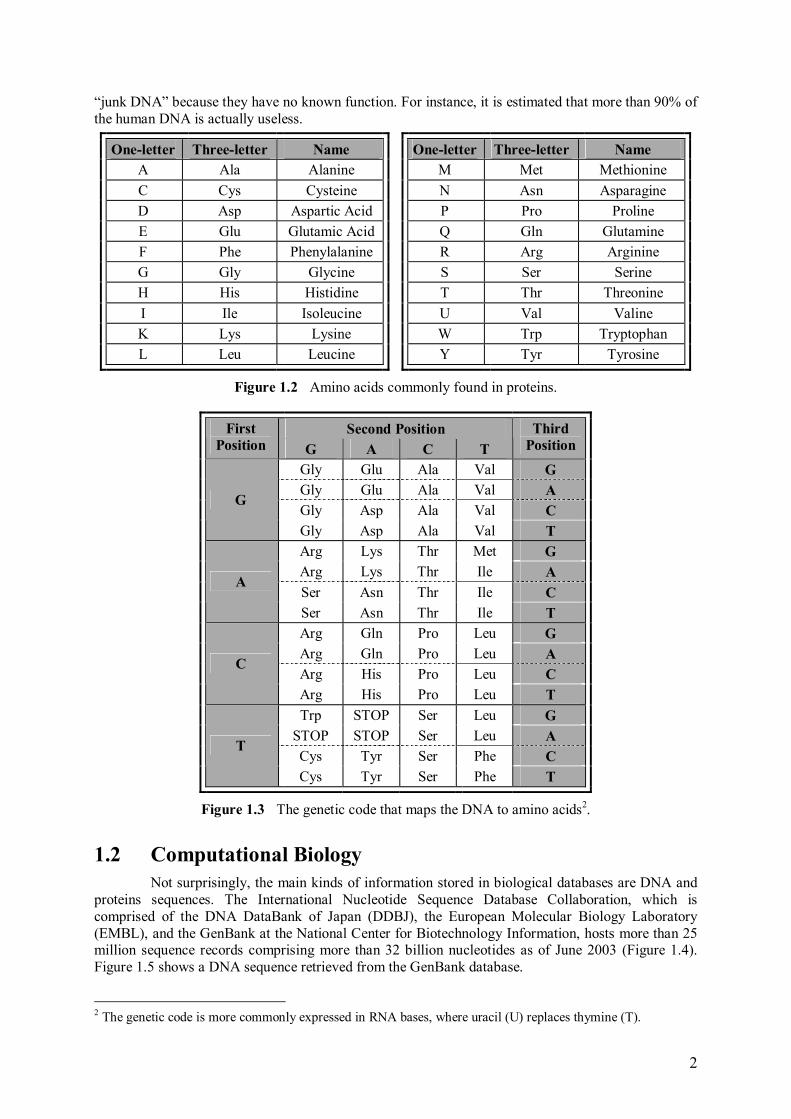
Proteins, roughly speaking, are responsible for what a living being is and does in a physical sense [27]. They are the molecules that accomplish most of the functions of a living cell [17], determining its shape and structure. Again, a protein is a linear sequence of simpler molecules called amino acids. Twenty different amino acids are commonly found in proteins, and they are identified by a letter of the alphabet or a three-letter code (Figure 1.2). For instance, alanine, one the most frequently appearing amino acids, is represented by the letter A or the three-letter code Ala. Like the DNA, proteins are conveniently represented as a string of letters expressing its sequence of amino acids. There is an intimate relation between DNA and proteins sequences. To produce a protein, the cell �reads� a sequence of three nucleotides from the DNA string, called a codon, to generate each of its amino acids. For instance, the triplet AAG, when found in a DNA strand, instructs the cell to generate the lysine amino acid. The correspondence between codons and amino acids is known as the genetic code (Figure 1.3). The genetic code includes three special codons (the �STOP� entries in the figure) used to indicate the end of a gene. A gene is a contiguous stretch along the DNA that encodes a protein. Genes are sometimes composed of alternating segments called introns and exons. The introns are spliced out during the process of protein generation and, therefore, have no influence on protein synthesis. Surprisingly, not all parts of a DNA molecule encode genes; some segments are called

2

�junk DNA� because they have no known function. For instance, it is estimated that more than 90% of the human DNA is actually useless.

One-letter Three-letter Name One-letter Three-letter Name A Ala Alanine M Met Methionine C Cys Cysteine N Asn Asparagine D Asp Aspartic Acid P Pro Proline E Glu Glutamic Acid Q Gln Glutamine F Phe Phenylalanine R Arg Arginine G Gly Glycine S Ser Serine H His Histidine T Thr Threonine I Ile Isoleucine U Val Valine K Lys Lysine W Trp Tryptophan L Leu Leucine Y Tyr Tyrosine

Figure 1.2 Amino acids commonly found in proteins.

Second Position First Position G A C T

Third Position

Gly Glu Ala Val G Gly Glu Ala Val A Gly Asp Ala Val C

G

Gly Asp Ala Val T Arg Lys Thr Met G Arg Lys Thr Ile A Ser Asn Thr Ile C

A

Ser Asn Thr Ile T Arg Gln Pro Leu G Arg Gln Pro Leu A Arg His Pro Leu C

C

Arg His Pro Leu T Trp STOP Ser Leu G

STOP STOP Ser Leu A Cys Tyr Ser Phe C

T

Cys Tyr Ser Phe T

Figure 1.3 The genetic code that maps the DNA to amino acids2.

1.2 Computational Biology Not surprisingly, the main kinds of information stored in biological databases are DNA and

proteins sequences. The International Nucleotide Sequence Database Collaboration, which is comprised of the DNA DataBank of Japan (DDBJ), the European Molecular Biology Laboratory (EMBL), and the GenBank at the National Center for Biotechnology Information, hosts more than 25 million sequence records comprising more than 32 billion nucleotides as of June 2003 (Figure 1.4). Figure 1.5 shows a DNA sequence retrieved from the GenBank database.

2 The genetic code is more commonly expressed in RNA bases, where uracil (U) replaces thymine (T).

3

Figure 1.4 Nucleotide sequence database growth (GenBank, DDBJ and EMBL).

In fact, this vast amount of data is perhaps the main tool of study in molecular biology today; and one of the most powerful methods of investigation employed by biologists is precisely the comparison of two biomolecular sequences because high sequence similarity usually implies significant functional or structural similarity [14]. As Gusfield further elucidates, �evolution reuses, builds on, duplicates, and modifies �successful� structures (proteins, exons, DNA regulatory sequences, morphological features, enzymatic pathways, etc.). Life is based on a repertoire of structured and interrelated molecular building blocks that are shared and passed around�. Lander remarks that �comparative DNA sequencing will unlock the record of 3.5 billion years of evolutionary experimentation. It will not only reveal the precise branches in the tree of life, but will elucidate the timing and character of major evolutionary innovation. (...) Sequence differences hold the key to understanding how nature generates such diversity of form and function with such an economy of genes � producing, for example, elephants, gazelles, mice and humans from the same basic mammalian repertoire of genes� [20].

>gi|21326584|ref|NC_003977.1| Hepatitis B virus, complete genome CTCCACAACATTCCACCAAGCTCTGCTAGATCCCAGAGTGAGGGGCCTATATTTTCCTGCTGGTGGCTCC

AGTTCCGGAACAGTAAACCCTGTTCCGACTACTGCCTCACCCATATCGTCAATCTTCTCGAGGACTGGGG

ACCCTGCACCGAACATGGAGAGCACAACATCAGGATTCCTAGGACCCCTGCTCGTGTTACAGGCGGGGTT TTTCTTGTTGACAAGAATCCTCACAATACCACAGAGTCTAGACTCGTGGTGGACTTCTCTCAATTTTCTA

GGGGGAGCACCCACGTGTCCTGGCCAAAATTCGCAGTCCCCAACCTCCAATCACTCACCAACCTCTTGTC

CTCCAACTTGTCCTGGCTATCGCTGGATGTGTCTGCGGCGTTTTATCATATTCCTCTTCATCCTGCTGCT

Figure 1.5 Partial sequence of the Hepatitis B virus� genome retrieved from the GenBank database3.

Sequence comparison can be defined as the problem of finding which parts of the sequences are similar and which parts are different. It is regarded as the building block for many other, more complex problems such as multiple alignments (the comparison of a group of related sequences) and the construction of phylogenetic trees that explain the evolutionary relationship among species. Sequence comparison is actually a well-know problem in computer science. For the computer scientist, biomolecular sequences are just another source of data. Indeed, one that has experienced a tremendous growth in interest to the point that it has spawned an interdisciplinary field of its own, generally know as bioinformatics, computational molecular biology or just computational biology. As biological databases grow in size, faster algorithms and tools are needed. This work will concentrate on efficient algorithms for comparing two sequences.

3 In FASTA format.

4

2 Sequence Comparison

As observed in chapter 1, our interest when we compare two sequences is to identify similarities and differences between them. Generally, a measure of how similar they are is also desirable. A typical approach to solve this problem is to find a good and plausible alignment between the two sequences. Then, given an appropriate scoring scheme, their similarity can be computed.

In section 2.1 the notions of similarity and alignment are examined in depth. Section 2.2 describes standard algorithms for solving the alignment problem whereas section 2.3 shows how these solutions can be improved. Finally, section 2.4 addresses efficient algorithms for the alignment problem.

2.1 Sequence Alignment and Similarity The idea of aligning two sequences (of possibly different sizes) is to write one on top of the

other, and �break� them into smaller pieces by inserting spaces in one or the other so that identical subsequences are eventually aligned in a one-to-one correspondence � naturally, spaces are not inserted in both sequences at the same position. In the end, the sequences end up with the same size. The following example illustrates an alignment between the sequences A=�ACAAGACAGCGT� and B=�AGAACAAGGCGT�.

A = ACAAGACAG-CGT | || | || ||| B = AGAACA-AGGCGT

Figure 2.1 Alignment of two sequences.

The objective is to match identical subsequences as far as possible. In the example, nine matches are highlighted with vertical bars. However, if the sequences are not identical, mismatches are likely to occur as different letters are aligned together. Two mismatches can be identified in the example: a �C� of A aligned with a �G� of B, and a �G� of A aligned with a �C� of B. The insertion of spaces produced gaps in the sequences. They were important to allow a good alignment between the last three characters of both sequences.

An alignment can bee seen as a way of transforming one sequence into the other. From this point of view, a mismatch is regarded as a substitution of characters. A gap in the first sequence is considered an insertion of a character from the second sequence into the first one, whereas a gap in the second sequence is considered a deletion of a character of the first sequence. In the previous example, A can be converted into B in four steps: 1) substitute the first �C� for a �G�; 2) substitute the first �G� for a �C�; 3) delete the second �C�; and 4) insert a �G� before the last three characters.

Once the alignment is produced, a score can be assigned to each pair of aligned letters, called aligned pair, according to a chosen scoring scheme. We usually reward matches and penalize mismatches and gaps. The overall score of the alignment can then be computed by adding up the score of each pair of letters. For instance, using a scoring scheme that gives a +1 value to matches and −1 to mismatches and gaps, the alignment of Figure 2.1 scores 9 · (1) + 2 · (−1) + 2 · (−1) = 5.

The similarity of two sequences can be defined as the best score among all possible alignments between them. Note that it depends on the choice of scoring scheme. In the next sections, the problem of finding the best alignment of two sequences (an alignment that gives the highest score) will be addressed. A related notion is that of distance. However, this work will focus on similarity, as it is the preferred choice for biological applications.

Thus far, this section has described a type of alignment know as global alignment since we are interested in the best match covering the two sequences in their entirety. Frequently, though, biologists are interested in short regions of local similarity. A local alignment is one that looks for best alignments between �pieces�, or more precisely, substrings of both sequences.

5

2.1.2 Substitution Matrices In the previous example, fixed scores were given for matches, mismatches and gap penalties.

However, biologists frequently use scoring schemes that take into account physicochemical properties or evolutionary knowledge of the sequences being aligned. This is common when protein sequences are compared. For instance, for some reason one might want to penalize the mismatch of an aspartic acid (D) with leucine (L) more heavily than a mismatch between the same aspartic acid with, say, histidine (H). Similarly, one may want to reward a match of two cysteines (C) better than two alanines (A).

This type of scoring schemes is called alphabet-weight scoring schemes, and is usually implemented by a substitution matrix. Currently, two types of amino acid substitution matrices are being largely used by biologists for practical protein sequence alignment: PAM and BLOSUM. They were developed from different concepts but have the same structure. In fact, they are a series of matrices with varied degrees of sensibility.

The PAM matrices (acronym for point accepted mutations) are extrapolated from data obtained from very similar sequences to reflect an amount of evolution producing on average one mutation per hundred amino acids. The BLOSUM matrices (acronym for blocks substitution matrix), in contrast, were developed to detect more distant relationships [14]. In particular, BLOSUM50 and BLOSUM62 are being widely used for pairwise alignment and database searching [12].

Substitution matrices allow for the possibility of giving a positive score for a mismatch, what is sometimes called an approximate or partial match. For instance, the BLOSUM62 matrix returns a score of +2 for the substitution of a lysine (K) for an arginine (R).

2.2 Standard Algorithms In the previous section, the similarity of two sequences was defined as the best score among

all possible alignments between them. Examining every alternative can be virtually impossible unless the sequences are relatively short, because the number of potential alignments is exponential. Fortunately, there are simpler solutions that yield much more efficient algorithms.

2.2.1 Needleman-Wunsch The standard global alignment algorithm, referred to as Needleman-Wunsch [25] after its

original authors4, computes the similarity between two sequences A and B of lengths m and n, respectively, using a dynamic programming approach. Dynamic programming is a strategy of building a solution gradually using simple recurrences [8]. The key observation for the alignment problem is that the similarity between sequences A[1..n] and B[1..m] can be computed by taking the maximum of the three following values:

• the similarity of A[1..n −1] and B[1..m −1] plus the score of substituting A[n] for B[m]; • the similarity of A[1..n −1] and B[1..m] plus the score of deleting aligning A[n]; • the similarity of A[1..n] and B[1..m −1] plus the score of inserting B[m].

From this observation, the following recurrence can be derived: sim ( A[1..i], B[1..j] ) = max { sim ( A[1..i −1], B[1..j −1] ) + sub ( A[i], B[j] ); sim ( A[1..i −1], B[1..j] ) + del ( A[i] ); sim ( A[1..i], B[1..j −1] ) + ins ( B[j] ) } where sim (A, B) is a function that gives the similarity of two sequences A and B, and sub

(a, b), del (c) and ins (c) are scoring functions that give the score of a substitution of character a for character b, a deletion of character c, and an insertion of character c, respectively. This recurrence is complete with the following base case:

sim ( A[0], B[0] ) = 0;

4 The algorithm described here is, in reality, an improved variant of their original work.

6

where A[0] and B[0] are defined as empty strings. To solve the problem with this recurrence, the algorithm build an (n +1) × (m +1) matrix M

where each M[i, j] represents the similarity between sequences A[1..i] and B[1..j] (Figure 2.2). The first row and the first column represent alignments of one sequence with spaces. M[0, 0]

represents the alignment of two empty strings, and is set to zero. All other entries are computed with the following formula:

M[i, j] = max { M[i −1, j −1] + sub ( A[i], B[j] ); M[i −1, j] + del ( A[i] ); M [i, j −1] + ins ( B[j] ) } The matrix can be computed either row by row (left to right) or column by column (top to

bottom). In the end, M[n, m] will contain the similarity score of the two sequences. Since there are (m+1) · (n+1) positions to compute and each take a constant amount of work, this algorithm has time complexity of O(n2). Clearly, it has also quadratic space complexity since it needs to keep the entire matrix in memory.

0 1 2 3 4 5 6 7 8 9 10 11 12 - A G A A C A A G G C G T 0 - 0 -1 -2 -3 -4 -5 -6 -7 -8 -9 -10 -11 -12 1 A -1 1 0 -1 -2 -3 -4 -5 -6 -7 -8 -9 -10 2 C -2 0 0 -1 -2 -1 -2 -3 -4 -5 -6 -7 -8 3 A -3 -1 -1 1 0 -1 0 -1 -2 -3 -4 -5 -6 4 A -4 -2 -2 0 2 1 0 1 0 -1 -2 -3 -4 5 G -5 -3 -1 -1 1 1 0 0 2 1 0 -1 -2 6 A -6 -4 -2 0 0 0 2 1 1 1 0 -1 0 7 C -7 -5 -3 -1 -1 1 1 1 0 0 2 1 0 8 A -8 -6 -4 -2 0 0 2 2 1 0 1 1 2 9 G -9 -7 -5 -3 -1 -1 1 1 3 2 1 2 1

10 C -10 -8 -6 -4 -2 0 0 0 2 2 3 2 1 11 G -11 -9 -7 -5 -3 -1 -1 -1 1 3 2 4 3 12 T -12 -10 -8 -6 -4 -2 0 0 0 2 2 3 5

Figure 2.2 Standard dynamic programming matrix for the global alignment of sequences A=�ACAAGACAGCGT� and B=�AGAACAAGGCGT� with paths to retrieve optimal alignments indicated with arrows.

Once the matrix has been computed, the actual alignment can be retrieved by tracing a path in the matrix from the last position to the first (Figure 2.2). The trace is a simple procedure that compares the value at each M[i, j] to the values of its left, top and diagonal entries according to the formula given above. For instance, if M[i, j] = M [i, j −1] + ins ( B[j] ), the trace reports an insertion of character B[j] and proceeds to entry M[i, j −1]. Alternatively, pointers can be saved on each entry during the computation of the matrix so that this evaluation step can be avoided at the cost of more memory usage. Since the path can be as long as O(m + n), this procedure has linear time complexity. Note that sometimes more than one path can be traversed and, as a result, multiple high-scoring alignments can be produced. In the matrix of Figure 2.2, two optimal alignments can be retrieved (Figure 2.1 and Figure 2.3).

A = ACAAGACA-GCGT | || | | |||| B = AGAACA-AGGCGT

Figure 2.3 Another optimal alignment retrievable from the matrix of Figure 2.2.

7

It is often useful to see the dynamic programming solution for the sequence alignment problem as a directed weighted graph with (n +1) × (m +1) nodes representing each entry (i, j) of the matrix, and having the following edges:

• ((i −1, j −1), (i, j)) with weight equals to sub ( A[i], B[j] ); • ((i −1, j), (i, j)) with weight equals to del ( A[i] ); • ((i, j −1), (i, j)) with weight equals to ins ( B[j] );

A path from node (0, 0) to (n, m) in the alignment graph corresponds to an alignment between the two sequences, and the problem of retrieving an optimal alignment is converted to the problem of finding a path in the graph with highest weight.

2.2.2 Smith-Waterman In section 2.1, a local alignment was defined as the problem of finding the best alignment

between substrings of both sequences. In 1981, T. F. Smith and M. S. Waterman [29] showed that a local alignment can be computed using essentially the same idea employed by Needleman and Wunsch. The main difference is that M[i, j] contains the similarity between suffixes of A[1..i] and B[1..j]. As a result, the recurrence relation is slightly altered because an empty string is a suffix of any sequence and, therefore, a score of zero is always possible. The formula for computing M[i, j] becomes:

M[i, j] = max { 0; M[i −1, j −1] + sub ( A[i], B[j] ); M[i −1, j] + del ( A[i] ); M[i, j −1] + ins ( B[j] ) } Another important distinction is that the score of the best local alignment is the highest value

found anywhere in the matrix. This position is the starting point for retrieving an optimal alignment using the same procedure described for the global alignment case. The path ends, however, as soon an entry with score zero is reached. It is trivial to see that the Smith-Waterman algorithm has the same time and space complexity as the Needleman-Wunsch.

2.2.3 A Note on Gap Penalty Functions The alignments algorithms described in sections 2.2.1 and 2.2.2 assume that gap costs are

given by a constant gap penalty function5. This means that a gap is given the same score no matter how long it is. However, biologists have long recognised that insertions and deletions generally do not occur a single base at a time. Therefore, when biomolecular sequences are compared, it is commonly accepted that a gap of k spaces is more likely to appear than k incidences of a single gap spread across the sequences. In order to make this distinction, a general gap penalty function is needed so that the cost of a gap is a function of its length. Unfortunately, if a general gap penalty function is required, it is not possible to compute an alignment with the algorithms described earlier because the scoring scheme is no longer additive. Moreover, the solution to such a problem has complexity O(n3) [27].

A more restrictive function, called affine gap penalty function6, allows an O(n2) solution at the same time that it is still able to distinguish between a gap of k spaces and k isolated gaps by penalising two events independently, the opening and the extension of a gap. It is important to observe that a constant gap penalty function is as a special case of an affine function in which the cost of opening a gap is zero. Although the affine model is probably the most common function used in practice, this work is focused on algorithms with constant gap penalty functions.

5 Also called linear or additive. 6 Sometimes confusingly called linear.

8

2.3 Reducing Space Complexity If the similarity value only is needed (and not the alignment itself), it is easy to reduce the

space requirement of both Needleman-Wunsch and Smith-Waterman algorithms to O(n) by keeping in memory just the last row or column of the matrix.

If the alignment is needed, a divide-and-conquer refinement due to D. Hirschberg7 [16] can be applied. The idea is to divide the matrix into two halves at its middle row i, and to compute the top submatrix as usual, from its leftmost top entry to its rightmost bottom one, keeping just the last row in memory. Then, the bottom matrix computed in a reversed direction, from the rightmost bottom entry to the leftmost top one, again keeping the last row only.

When these two computations meet, the score of both rows at each column is added, and the column k with maximum score is chosen. M[i, k] is then guaranteed to be in the path of an optimal alignment and the problem is reduced to submatrices A[0..i-1, 0..k-1] and B[i + 1..n, k + 1..m] that are computed recursively. Note that, although this algorithm does not worsen the quadratic time complexity, it roughly doubles the running time.

2.4 Using Compression A different strategy is used by Crochemore, Landau and Ziv-Ukelson to improve the

standard algorithms in terms of time and space complexity from O(n2) to O(n2/log n) using Lempel-Ziv data compression techniques.

The complexity is actually O(h · n2 / log n), where 0 ≤ h ≤ 1 is a real number denoting the entropy of the text (a measure of how compressible it is). The number h is small when the text has a lot of order (and, consequently, is highly compressible) and large when it has a lot of disorder [6]. This means that, the more compressible a sequence is, the less memory the algorithm will require, and the faster it will run.

Two versions of the algorithm are given by Crochemore et al., one for global alignment and one for local alignment. In section 2.4.1, the global alignment version will be examined, while section 2.4.4 will describe the changes and extensions required to compute a local alignment employing the same concept. It is important to note that description of the algorithms given here are not comprehensive. Instead, the objective is to give a general idea and focus on the most relevant issues, especially those concerning their implementation. For a more detailed description, the interested reader is referred to the original paper �A Sub-quadratic Sequence Alignment Algorithm for Unrestricted Scoring Matrices� [9].

2.4.1 Global Alignment The idea behind the improvement achieved by Crochemore et al. is to identify repetitions in

the sequences and reuse previous computation of their alignments. The first step is, therefore, to parse the sequences into LZ78-like factors. LZ78 is a popular dictionary-based compression algorithm designed by J. Ziv and A. Lempel [30]. It works by recognizing repetitions in the text and replacing them with references to previous phrases stored in a dictionary. The text is actually encoded as a series of factors where each factor is a pointer to the longest phrase previously seen plus one character. For instance, the sequence B=�AGAACAAGGCGT� is parsed into eight factors as illustrated by Figure 2.4. The LZ78 algorithm is said to be prefix closed, i.e. all prefixes of phrase in the dictionary are also in the dictionary. This property implies that it can be implemented as a tree. Indeed, the factorisation can be easily accomplished with the help of a trie8, or digital search tree (Figure 2.6).

Once the sequences are parsed, the algorithm builds a matrix of blocks, called block table, which is a partition of the alignment graph. Each entry (i, j) of the block table corresponds to an alignment between factor i from the first sequence and factor j from the second sequence.

7 An alternative formulation is given by Durbin et al. in [12]. 8 A more detailed description of the trie data structure is given in section 4.1.

9

Consider a block G in which the factor xa from sequence A is aligned with factor yb from sequence B (Figure 2.5). Here, xa extends a previous factor of A with character a, while yb extends a previous factor of B with character b. The input border of G is defined as the set of values at its left and top borders. Similarly, the output border is defined as the set of values at its right and bottom borders. If ℓr is the number of characters of xa and ℓc the number of characters of yb, the size of both the input and output borders of a block are t = ℓr + ℓc + 1. Furthermore, the following prefix blocks of G can be distinguished:

• Left prefix: the block that contains the alignment of factor xa of A with factor y of B; • Top prefix: the block that contains the alignment of factor x of A with factor yb of B; • Diagonal prefix: the block that contains the alignment of factor x of A with factor y of B.

Note that each factor has a pointer to its prefix factor, called ancestor. This pointer allows the retrieval of prefix blocks of G from the block table in constant time. Rather than computing each value of the alignment block G, the algorithm only computes the values on the output border, and this is precisely what makes it more efficient. The computation proceeds in two phases: encoding and propagation.

In the encoding phase, the structure of a block G is studied and represented in an efficient way by computing weights of optimal paths connecting each entry of the input border to each entry of the output border. This information is encoded in a matrix, called DIST matrix, such that DIST[i, j] stores the weight of an optimal paths connecting entry i of the input border to entry j the output border (Figure 2.7). The crucial observation is that, in the corresponding alignment graph, the block G has the same structure of its prefix blocks except for the new vertex that compares character a of A with character b of B. This means that all but one column of the DIST matrix can be copied from prefix blocks.

Serial number Factor Phrase encoded0 empty (empty string) 1 ( 0 , A ) A 2 ( 0 , G ) G 3 ( 1 , A ) AA 4 ( 0 , C ) C 5 ( 3 , G ) AAG 6 ( 2 , C ) GC 7 ( 2 , T ) GT

Figure 2.4 Lempel-Ziv factors (LZ78) of sequence B=�AGAACAAGGCGT�.

The only column that needs to be computed is the column ℓc that contains the weights of optimal paths from input border entries to the new cell. Columns to the left of ℓc are retrieved recursively from left prefix blocks. Similarly, columns to the right of ℓc are retrieved from top prefix blocks. For this reason, each block only needs to store one column of the DIST martrix. The DIST matrix of a block can then be assembled as an array of pointers to DIST columns of prefix blocks (Figure 2.6), and discarded after the computation of the output border.

Each entry i of column ℓc contains the score of the best path from entry i in the input border to entry ℓc of the output border. It is set to the maximum among the following values:

• entry i of the DIST column for the left prefix plus the score of deleting character a; • entry i of the DIST column for the diagonal block plus the score of substituting a for b; • entry i of the DIST column for the top prefix plus the score of inserting character b;

In the propagation phase, the input border of a block G is retrieved from the output border of the left and top blocks of G. Then, a matrix defined as OUT[i, j] = I[i] + DIST[i, j] where I is the input

10

border array, is constructed. In other words, the OUT matrix is the DIST matrix updated by the input border of a block (Figure 2.7).

Finally, the output border is computed by taking the maximum value of each column of the OUT matrix (Figure 2.7). A naive approach to compute the output border of a block from the OUT matrix of size t × t would take a time proportional to O(t2) and would destroy the efficiency of the algorithm. However, Aggarwal and Park [2] observed that the DIST matrix is a Monge array and hence totally monotone. The OUT matrix, as it was defined, enjoys the same property. Fortunately, an algorithm due to Aggarwal et al. [1], nicknamed SMAWK, is able to compute all column maxima of a totally monotone array in linear time. Therefore, by using SMAWK, the output border a block can be computed in time O(t).

0 1 2 3 4 5 6 7 - A G A A C A A G G C G T 0 - 0 -1 -2 -3 -4 -5 -6 -7 -8 -9 -10 -11 -12 1 A -1 1 0 -1 -2 -3 -4 -5 -6 -7 -8 -9 -10 2 C -2 0 0 -1 -2 -1 -2 -3 -4 -5 -6 -7 -8

A -3 -1 -1 0 -1 -2 -4 -6 3 A -4 -2 -2 0 2 1 0 1 0 -1 -2 -3 -4

4 G -5 -3 -1 -1 1 1 0 0 2 1 0 -1 -2 A -6 -4 -2 0 1 0 0 5 C -7 -5 -3 -1 -1 1 1 1 0 0 2 1 0 A -8 -6 -4 0 0 1 1 2

6 G -9 -7 -5 -3 -1 -1 1 1 3. 2 1 2 1 C -10 -8 -6 -2 0 2. 3 1 7 G -11 -9 -7 -5 -3 -1. -1. -1. 1. 3 2 4 3

8 T -12 -10 -8 -6 -4 -2 0 0 0 2 2 3 5

Figure 2.5 Matrix partitioned by the Lempel-Ziv factorisation for a global alignment of sequences A=�ACAAGACAGCGT� and B=�AGAACAAGGCGT�. Entries that are not computed are left blank. The block corresponding to the alignment of factors �CG� and �AAG� is highlighted with a thicker border. Its input border is shown in shaded boxes while the output border values have a dotted line around them. Prefix blocks are indicated with double borders.

2.4.2 Analysis of Complexity The time and space complexity of the algorithm depends essentially on the number of blocks

and the size of their borders. It has been proved that the Lempel-Ziv factorisation has linear time complexity and an upper bound of O(h · n/ log n) on the number of generated factors, where h is the entropy of the text and n is its length. Therefore, no more than O(h2 · n2 / log2 n) blocks are created. The computation at each block consists of:

• computing the new DIST column; • retrieving the input border; • encoding the DIST and OUT matrices; • computing the output border;

All of these tasks take time and space proportional to t, the size of the output border. For a given row or column of the block table, the length of all output borders put together is O(n). Hence, there are O(h · n/ log n) rows of length O(n) and O(h · n/ log n) columns of length O(n), and the total space and time complexity is O(h · n2 / log n).

Crochemore et al. claim that their algorithms are the first to achieve sub-quadratic time complexity with unrestricted scoring schemes. According to them, the only previous algorithm to achieve such a result, developed by Masek and Paterson [24], also divides the matrix into blocks, in

11

that case based on the Four Russians paradigm. However, that algorithm has the downside of requiring the scoring matrix to have rational numbers only. The algorithms of Crochemore et al., on the other hand, support unrestricted scoring matrices. They also noted that their algorithms are the first to work with fully compressed sequences, which might be useful when the sequences are retrieved in compressed format.

Block Table Trie for A Trie for B 0 1 2 3 4 5

0 1 2 3 4 5 6 7 DIST

0 -1 -2 -3 -1 -1 -2 -1 -3 -2 -2 -2 -1 -3 -3 -2 -2 0 -2 -2 -2 0 -1 -1 -2 -1 0

Figure 2.6 Assembling the DIST matrix from prefix blocks. The only column that needs to be computed is highlighted in shaded boxes. The other columns are retrieved from left and top prefix blocks. Partial tries for sequences A=�ACAAGACAGCGT� and B=�AGAACAAGGCGT� are shown on top right of the figure.

2.4.3 Alignment Recovery The process of retrieving an optimal alignment from the computed block table resembles that

of the standard algorithms. However, in order to enable such a recovery in time proportional to its length, extra information needs to be stored at each block:

• source: an array such that source[i] contains the index of the input border entry that is the source of the path with highest score to entry i of the output border;

• ancestor: an array such that ancestor[i] contains a pointer to the prefix block used to compute entry i of the output border;

• direction: an array that indicates the direction (whether left, diagonal or top) that must be followed to reach the source of the high-scoring path for each entry of the output border. All arrays are of size t and can be computed in O(t) time. Therefore, neither the space nor the

time complexity of the algorithm is compromised. The alignment recovery starts at entry (n, n) of the block table. At each stage, a block is

traversed by fetching the corresponding source of the high-scoring path from the source array. The appropriate prefix blocks are recursively retrieved from the ancestor array. The direction at each stage is given by the direction array. The procedure ends when the entry (0, 0) of the block table is reached.

DIST input border 0 1 2 3 4 5 -1 0 -1 -2 -3 ■ ■

0

1 2 4

3 5 6 7

0

1 2 4

3

5

6 7

A C G

TA C

G

G

A C G

A C

G

12

0 -1 -1 -2 -1 -3 ■ -1 -2 -2 -2 -1 -3 -3 1

► ■ -2 -2 0 -2 -2

1 ■ ■ -2 0 -1 -1 3 ■ ■ ■ -2 -1 0 ▼ -1 -2 -3 -4 ■ ■ -1 -1 -2 -1 -3 ■

-3 -3 -3 -2 -4 -4 OUT

■ -1 -1 1 -1 -1 ■ ■ -1 1 0 0 ■ ■ ■ 1 2 3

▼ output border -1 -1 -1 1 2 3

Figure 2.7 Output border of a block computed from its input border, DIST and OUT matrices. The ■ symbol at entry (i, j) indicates that no path exists from entry i of the input border to entry j of the output border. Column ℓc of the DIST matrix is highlighted in shaded boxes.

2.4.4 Local Alignment The local alignment problem can be solved with an extension of the algorithm described in

the previous sections. The main difference is that a path corresponding to an optimal alignment does not necessarily spans the entire block table. Instead, it may be contained entirely in a block, called C-path (Figure 2.8). If it is not a C-path, it can be characterized into three parts, in this order:

• a possibly empty S-path that starts in the middle of a block and ends at its output border; • zero or more block-crossing paths (paths that completely crosses a block); • a possibly empty E-path that starts at the input border of a block and ends inside it.

Therefore, the following data structures are needed to update the output border with possible optimal paths starting inside the block and to account for paths ending inside the block:

• E_path_score: an array containing the scores of the high-scoring E-paths starting at each entry of the input border;

• E_path_ancestor: an array of pointers to prefix blocks that are source of the high-scoring E-paths;

• E_path_ancestor_index: an array of indexes of the entries in the input border of a block that are source of the high-scoring E-path;

• path_type: an array that indicates the type of the high-scoring path ending at a given position of the output border;

• S_path_score: an array containing the value of the high-scoring path starting inside the block and ending at its output border;

• S_direction: the direction to the source of the S-path ending at the new cell of the block; • C: the score of the highest scoring path contained in this block (C-path).

As the block table is computed, the algorithm keeps track of the block containing the highest score as well as the type of the best path. The recovery routine starts at this position and proceeds in a similar way as explained in section 2.4.3 but also considering the other types of paths that may exist.

All data structures are arrays of size t except for the single variable S_direction and C, and their computation can be done in time proportional to t; hence, neither the time nor the space complexity of the algorithm is compromised.

13

Figure 2.8 Types of optimal paths in a local alignment.

C-path

Block-crossing path

E-path

S-path

14

3 Specification and Design

This chapter presents a library of computational biology algorithms, called NeoBio, developed as part of this work. It starts by describing its objectives in section 3.1 and its requirements in section 3.2. Section 3.3 addresses the rationale behind its design, and section 3.4 illustrates how the class library can be used.

3.1 Objectives The main objective of the development of NeoBio was to implement the sub-quadratic

algorithms for global and local sequence alignment proposed by Maxime Crochemore, Gad Landau and Michal Ziv-Ukelson in the paper �A Sub-quadratic Sequence Alignment Algorithm for Unrestricted Scoring Matrices� [9]. The algorithms were described in section 2.4.

The classical alignment algorithms of Needleman & Wunsch and Smith & Waterman (described in sections 2.2.1 and 2.2.2) have also been implemented. The advantages of implementing these were two-fold. Firstly, as they are the standard algorithms for pairwise sequence alignment, they served as a base for performance comparison, both in terms of memory usage and running time. Secondly, they were used to test the implementation of the algorithms of Crochemore et al. because they are simple and straightforward to code.

Although the present version consists mainly of pairwise sequence alignment algorithms, the library was developed in such a way that it can be extended in the future with other alignment algorithms as well as algorithms related to other areas of computational biology.

NeoBio was designed to study and evaluate sequence algorithms in the field of computational biology. There was no intention of providing real-world software utilities for practitioners in the field. The main reason is that, in real world, application�s requirements are much more complex. For example, biologists usually require a lot more of fine tuning options for sequence alignments, such as sequence filtering, that are beyond the scope of this project. Other requirements such as the generation of reports, for instance, would take too much time and distract the development from the central issues. Moreover, a number of software tools are available today such as the BLAST suite provided by the National Center for Biotechnology Information (briefly described in the section 5.1.1). It is important to note, however, that it is possible to extend the library to meet all the requirements of practical applications.

NeoBio was developed in Java for a number of reasons. Java is a modern and popular object oriented language and its source code arguably tends to be more readable than other languages such as C and C++. Indeed, the objective was to write short, clean, and simple code as far as possible. Efficiency was pursued as long as simplicity and readability of code was not compromised.

Although Java is sometimes criticised for being inefficient, recent developments in the language are enabling performances comparable to other languages such as C and C++, most notably the Java HotStpot Virtual Machine technology that employs optimization and compilation to native code on the fly. As an example, a recently-released sequence alignment software written entirely in Java, called PatterHunter (mentioned in section 5.1.1), claims to achieve better or at least as good performance as the best alignment tools available today.

3.2 Requirements The main requirement of the present version of NeoBio is to provide implementations of

following pairwise sequence alignment algorithms: Needleman & Wunsch (global alignment); Smith &Waterman (local alignment); Crochemore, Landau & Ziv-Ukelson for global alignment; and Crochemore, Landau & Ziv-Ukelson for local alignment. All implemented algorithms are designed to support constant gap penalty functions only. Simple tools must also be provided to allow the user to

15

compute and retrieve an optimal alignment and/or its score using the algorithms, either through GUI (graphical user interface) or through command line.

The library must separate the implementation of the algorithms and the user interface to allow for the possibility of modifying them independently. Moreover, all algorithms are required to implement the same interface so that they can be used interchangeably. In particular, they are required to respond to the following user events: 1) input of two sequences; 2) set of a scoring scheme; 3) request of an optimal alignment; 4) request of the score of an optimal alignment. There is no specific order to be followed by the user but, naturally, an optimal alignment or its score can only be requested after the sequences have been loaded and a scoring scheme has been set.

Algorithms must read the sequences in such a way that the input can come from any source such as files, network sockets or databases, provided certain conditions are met. Sequences can contain letters only although lines started with the greater-than symbol (�>�) are regarded as comments and must be completely skipped. White spaces (including tabs, line feeds and carriage returns) must also be ignored throughout. Note that, by accepting this format, the algorithms are also able to read sequences in FASTA format. FASTA is a format used by most sequence alignment software tools including those described in section 5.1.1.

All algorithms must produce the output in the same format containing all information necessary to display an optimal alignment: the score of the alignment, the two sequences with gaps, and a score tag line that indicates whether a match, a partial match, a mismatch or a gap occurs at each aligned pair. This output must be simple and such that future versions of NeoBio can provide report formatters that take this information as input to produce different kinds of reports. The alignments produced by two different algorithms of the same type (i.e. two local alignments or two global alignment algorithms) for a given scoring scheme and a pair of sequences must be coherent but not necessarily identical since any optimal alignment can be retrieved (recall that, sometimes, more than one optimal alignment is possible). Obviously, the score returned must be the same.

Algorithms should support two types of scoring schemes. The first one, called basic scoring scheme, is able to return three distinct values for each possible event: a match, a mismatch and a gap. The second type of scoring scheme, called scoring matrix, is an alphabet-weight scoring scheme where matches, mismatches and gaps are scored based on what characters are being aligned. This scoring scheme is aimed to represent substitution matrices, such as BLOSUM and PAM amino acid substitution matrices, and must be able to read those matrices in such a way that the input can come from any source. Scoring schemes must be configurable to consider or ignore the case of the characters. The two types of scoring schemes must have the same interface so that the sequence alignment algorithms can use them interchangeably.

3.3 Design This section will address the object-oriented design of the NeoBio class library, with a

description of the modules, classes and interfaces. The focus will be on the most important classes and the most relevant issues, therefore some details are deliberately omitted. Although some internal classes and interface are described, this section will concentrate primarily on services available through public interfaces (a complete documentation of the API is available for the developer interested in modifying or extending the library). The descriptions involve Java terms and syntax (set in Monospaced font) that will be simplified whenever possible. UML diagrams that illustrate the relationship between classes are also given in simplified forms. An effort was made to associate the rationale behind the design to the objectives and requirements described in the previous sections.

3.3.1 Modules In order to meet the requirement of separating the implementation of algorithms and the user

interface, the library was divided into three modules (or packages in Java jargon) that group related classes (Figure 3.1):

• alignment: contains classes that implement pairwise sequence alignment algorithms;

16

• textui: contains command line based tools to run the algorithms provided by other packages;

• gui: contains GUI tools to run the algorithms provided by other packages. The classes of the alignment package will be detailed in the following sections. The classes

contained in the textui and gui modules are briefly described in section 3.4.

Figure 3.1 Packages and classes.

3.3.2 Main Classes The alignment module consists primarily of classes that implement four pairwise sequence

alignment algorithms: • NeedlemanWunsch: implements the Needleman & Wunsch global alignment algorithm

described in section 2.2.1; • SmithWaterman: implements the Smith & Waterman local alignment algorithm described in

section 2.2.1; • CrochemoreLandauZivUkelsonGlobalAlignment: implements the global alignment

algorithm of Crochemore, Landau & Ziv-Ukelson described in section 2.4.1; • CrochemoreLandauZivUkelsonLocalAlignment: implements the local alignment algorithm

of Crochemore, Landau & Ziv-Ukelson described in section 2.4.4; The diagram of Figure 3.2 illustrates the relationship between these classes. Note that the

classes implementing the algorithms of Crochemore et al. derive from a common superclass. This superclass contains the data structures and methods pertinent to both versions of the algorithm. In order to achieve the requirement of having all algorithms implementing the same interface, all classes are extensions of the abstract class PairwiseAlignmentAlgorithm. This superclass specifies the following public interface that must be implemented by all algorithms:

17

• void loadSequences (Reader input1, Reader input2): load two sequences from the specified character input streams;

• void setScoringScheme (ScoringScheme scoring): sets the scoring scheme for computing alignments;

• int getScore (): return the score of a high-scoring alignment between the loaded sequences according to the scoring scheme previously set;

• PairwiseAlignment getPairwiseAlignment ():return a high-scoring alignment between the loaded sequences according to the scoring scheme previously set. The loadSequences method uses a generic Reader class provided by the core Java API for

reading characters from an input stream. This conforms to the requirement of reading a sequence from any input source such as a file or a network socket. The data can come from any source provided it is properly wrapped in a Reader object.

The getPairwiseAlignment method returns a PairwiseAlignment object that contains an optimal alignment and its score. The getScore method returns the score only. This allows for the possibility of using a more efficient method if the score only is needed. For instance, both NeedlemanWunsch and SmithWaterman classes have linear space algorithms to compute the score (in quadratic time) as described in section 2.3. If the alignment is required, these classes then employ the standard quadratic space (and time) algorithms. Note that the getScore and getPairwiseAlignment methods are common for both local and global alignment algorithms; the type of alignment returned (whether local or global) depends on what algorithm is used.

Figure 3.2 Overview of the alignment module.

The PairwiseAlignment class encapsulates an optimal alignment between two sequences produced by an alignment algorithm. All alignment algorithms produce their output in an instance of this class, which contains the following fields:

18

• String gapped_seq1: a String object with the first gapped sequence; • String gapped_seq2: a String object with the second gapped sequence; • String score_tag_line: a String object with the score tag line that indicates whether a

match, a partial match, a mismatch or a gap occurs at each position of the alignment; • int score: the score of this alignment.

These fields are declared as protected and, therefore, are not available directly. Instead, it is necessary to use a corresponding public get method: getGappedSequence1, getGappedSequence2, getScoreTagLine and getScore. Note that an instance of the PairwiseAlignment class is easily converted into a String representation through the toString method defined by the Java�s Object class.

Scoring schemes are implemented by the ScoringScheme class and its subclasses (Figure 3.2). The public interface defined by the superclass allows an alignment algorithm to use any scoring scheme regardless of how it is implemented. It consists of the following methods:

• int scoreDeletion (char a): returns the score of deleting character a; • int scoreInsertion (char a): returns the score of inserting character a; • int scoreSubstitution (char a, char b): returns the score of substituting character a

for character b; Two implementation of scoring schemes are available. The BasicScoringScheme class is

able to return three distinct values according to each possible event: a match, a mismatch and a gap. These values are supplied to the following constructor method:

• BasicScoringScheme (int match_reward, int mismatch_penalty, int gap_cost) The ScoringMatrix class is an alphabet-weight scoring scheme where matches, mismatches

and gaps are scored based on the characters being aligned. This scoring scheme represents substitution matrices, such as BLOSUM and PAM matrices. Matrices are loaded from any source encapsulated in a proper Reader input stream through the following constructor:

• ScoringMatrix (Reader input) All scoring schemes classes have alternative constructors that allow the user to specify if the

case of characters must be ignored or not.

3.4 Using Sequence Alignment Algorithms In order to use the alignment algorithms provided in the alignment package, four steps must

be followed. Firstly, it is necessary to create an instance of the chosen algorithm. The second steps consist of loading two sequences into the algorithm instance through the loadSequences method. The third step consists of building a scoring scheme and instructing the algorithm to use it through the setScoringScheme method. Finally, an optimal alignment or its score can be retrieved through the getScore or getPairwiseAlignment methods.

The example in Figure 3.3 illustrates a typical sequence of method calls for computing a global alignment with the Needleman & Wunsch algorithm. Note that it uses a ScoringMatrix scoring scheme with data loaded from a file called �BLOSUM62.txt�. The sequences are also loaded from files.

The NeoBio class library also provides simple tools that allow easy interaction with the algorithms. Two versions are currently available: a command line tool provided in the textui package and GUI application available in the gui package (a prototype is shown in Figure 3.4). Both have the same basic concept illustrated in Figure 3.3, and both provide the same features. In particular, they read sequences and scoring matrices from local files. The graphical interface is, naturally, easier to use. The text-based tool, however, consumes less memory and is generally faster.

19

// create an instance of an alignment algorithm

algorithm = new NeedlemanWunsch ();

// create a Reader wrapper for the sequences

seq1 = new FileReader (“sequence1.txt”);

seq2 = new FileReader (“sequence2.txt”);

// load sequences into the algorithm instance

algorithm.loadSequences (seq1, seq2);

// create a Reader wrapper for a scoring matrix file

matrix_file = new FileReader (“blosum62.txt”);

// create an instance of the scoring matrix class

matrix = new ScoringMatrix (matrix_file);

// set the scoring scheme to be used by the algorithm

algorithm.setScoringScheme (matrix);

// compute an optimal alignment

alignment = algorithm.getPairwiseAlignment();

// display the alignment System.out.println (alignment);

Figure 3.3 Using sequence alignment algorithms.

The text-based application requires the following arguments in the command line: • <algorithm>: either �NW� for Needleman & Wunsch, �SW� for Smith & Waterman,

�CLZG� for Crochemore, Landau & Ziv-Ukelson�s global alignment algorithm or �CLZL� for the local alignment version;

• <sequence1>: the first sequence filename; • <sequence2>: the second sequence filename; • M <matrix>: if using a scoring matrix stored in a file; • S <match> <mismatch> <gap>: if using a simple scoring scheme, where <match> is the

match reward value, <mismatch> is the mismatch penalty value and <gap> is the cost of a gap. Note that the choices of scoring schemes (whether �M� or �S�) are, of course, mutually

exclusive. Figure 3.5 illustrates the text-based application used to compute a global alignment between two protein sequences.

20

Figure 3.4 Prototype of a graphical user interface.

>java neobui.textui.NeoBio CLZG prot14a.txt prot14b.txt M blosum62.txt

Loading sequences...

[ Elapsed time: 20 milliseconds ]

Computing alignment...

[ Elapsed time: 30 milliseconds ]

Alignment:

MVHLGPKKPQARKGSMADVPKELMDEIHQLEDMFTVDSETLRKVVKHFIDELNKGLTKKGGN--

MVHLG QARKGSM VPKELM +I E +FTV +ETL+ V KHFI EL KGL+KKGGN

MVHLG----QARKGSM--VPKELMQQIENFEKIFTVPTETLQAVTKHFISELEKGLSKKGGNIP

Score: 179

Figure 3.5 Using the command line based tool to compute a global alignment between two protein sequences with the algorithm of Crochemore, Landau & Ziv-Ukelson using a BLOSUM62 matrix.

21

4 Implementation

This chapter will address the implementation of the sequence alignment algorithms provided by the NeoBio class library. The algorithms of Needleman & Wunsch and Smith & Waterman are rather straightforward to implement, and have already been extensively covered in the literature [12] [14] [21] [27]. For this reason, this chapter will concentrate on the most relevant issues regarding the implementation of the global and local alignment algorithms proposed by Crochemore, Landau & Ziv-Ukelson (described in section 2.4). The descriptions given here apply to both versions of the algorithm, unless stated otherwise.

4.1 Lempel-Ziv Factorisation As described in section 3.3.2, all classes implementing sequence alignment algorithms use

the loadSequences method to read a sequence from a given input stream. Each implementation, however, uses specific classes and data structures to store the sequences according to its own needs. For example, both NeedlemanWunsch and SmithWaterman classes store the sequences in instances of the CharSequence class. This class is essentially an array of characters that provides random access to any entry in constant time.

The classes implementing the algorithms of Crochemore et al., in contrast, use the FactorSequence class to parse a stream of characters into a list of LZ78 factors. Each factor contains a serial number, a pointer to its ancestor � the prefix of the encoded phrase � and the new character (Figure 4.1). Each factor also contains the phrase�s length and a pointer to the next factor.

As noted in section 2.4.1, the factorisation is accomplished with the help of a trie, or digital search tree (Figure 2.6), implemented by the Trie class (Figure 4.1). A trie is a multiway tree (each node can have multiple children) that represents a set of strings. Each edge is labelled by a character, and each path from the root represents a string described by the characters labelling the traversed edges. There is a unique path from the root for each represented string.

The Trie class is defined recursively, i.e. each node is an instance of a Trie that has other Trie instances as children. Each node also contains data encapsulated in an object instance. In fact, there are many ways to implement a trie. Multiple pointers usually have the drawback of wasting space if the tree is not complete. In order to avoid this problem, a linked list approach is used. Each node only contains a pointer to the first child and a pointer to the next sibling, along with the corresponding character that labels each edge (Figure 4.2). In this way, a trie is a binary tree. Although this implementation is more efficient in terms of space, the search for an edge labelled with a given character is not constant, but proportional to the number of children.

It is easy to see that, in a trie, strings with common prefixes branch off from each other at the first distinguishing character. This is the feature explored by the FactorSequence class to represent the phrases of a sequence in such a way that it is easy to find the longest phrase already encoded. Each node in the trie is stores a phrase of the sequence encapsulated in an instance of the Factor class. For example, node 5 in Figure 4.2 contains factor (3, G) (compare with Figure 2.4).

In order to identify the longest encoded phrase, the trie is traversed from the root node as each character is read from the input stream. Eventually, the path reaches a node n where it cannot be extended. The trie�s properties guarantee that node n contains the longest phrase of the sequence parsed so far. At this point, a new factor is created and the trie is augmented with the new character.

To illustrate this process, suppose the FactorSequence class has read sequence B to the point of building the trie of Figure 2.4. At this point, the first twelve characters have been read. Furthermore, assume sequence B is �AGAACAAGGCGTAAC�. The objective is to read the longest sequence of characters already encoded by traversing a path in the trie from the root (node 0). The first character is an �A�, which allows the path to proceed to node 1. The next character is another �A� that extends the path to node 3. The next character is a �C� but there is no edge labelled with a �C� leaving

22

node 3. This means that �AA� is the longest phrase encoded in the trie. Consequently, factor (3, C) is created. Moreover, the trie is augmented with node 8 containing the new factor and a new edge from node 3 to node 8 labelled with a �C�.

Figure 4.1 Classes for the LZ78 factorisation.

Figure 4.2 Trie for the sequence B = �AGAACAAGGCGT� as it is implemented (compare with Figure 2.6).

4.2 Building the Block Table Once the sequence is parsed, the next step is to build the block table. As described in section

2.4.1, the block table is a matrix of alignment blocks. Each block contains the alignment of one factor of each sequence, and is stored in an instance of the AlignmentBlock class for global alignments, or LocalAlignmentBlock for local alignments (Figure 4.3).

Although the block table is built in the same way for both versions of the algorithm, the computation of each block depends whether a local or global alignment is being sought. For this reason, the CrochemoreLandauZivUkelson superclass has a general outline of how the block table is computed (Figure 4.4).

GA

C

T3

5

2 4

6 7

CA

G

0

1

23

Figure 4.3 AlingmentBlock and LocalAlingmentBlock classes.

The superclass does not compute each block, instead, it request subclasses to do so. This is accomplished by defining the following methods that must be provided by the subclasses:

• AlignmentBlock createRootBlock (Factor factor1, Factor factor2): computes the block at the first row and first column of the block table;

• AlignmentBlock createFirstRowBlock (Factor factor1, Factor factor2, int

col): computes a block at the first row of the block table, which corresponds to an alignment between one factor of sequence 2 and an empty string;

• AlignmentBlock createFirstColumnBlock(Factor factor1, Factor factor2, int

row): computes a block at the first column of the block table, which corresponds to an alignment between one factor of sequence 1 and an empty string;

• AlignmentBlock createBlock (Factor factor1, Factor factor2, int row, int

col): computes a block that corresponds to an alignment between one factor of sequence 1 and one factor of sequence 2. As implied by the methods� names and signatures, subclasses must not only compute a

block, but also create and return it in an instance of the AlignmentBlock class (or any subclass such as the LocalAlignmentBlock in the case of a local alignment).

4.3 Computing Alignment Blocks In general terms, the process of computing an alignment block consists of:

• computing the new DIST column; • retrieving the input border; • encoding the DIST and OUT matrices; • computing the output border.

The first step is rather simple to implement. Each entry in the DIST column is computed from the values of the left, diagonal and top prefix blocks by the taking the maximum of three values as described in section 2.4. This is precisely what is accomplished by the createBlock method illustrated in Figure 4.5. As it can be seen in Figure 4.5, the last three steps are delegated to the computeOutputBorder method show in Figure 4.6.

24

// create block table

block_table = new AlignmentBlock[num_rows][num_cols];

// start at the root of each trie

factor1 = seq1.getRootFactor();

factor2 = seq2.getRootFactor();

// initiate first cell of block table

block_table[0][0] = createRootBlock (factor1, factor2);

// compute first row

for (c = 1; c < num_cols; c++)

{ factor2 = factor2.getNext();

block_table[0][c] = createFirstRowBlock (factor1, factor2, c);

}

// compute remaining rows for (r = 1; r < num_rows; r++)

{

factor1 = factor1.getNext();

// go back to the root of sequence 2 factor2 = seq2.getRootFactor();

// compute first column of current row

block_table[r][0] = createFirstColumnBlock (factor1, factor2, r);

for (c = 1; c < num_cols; c++) {

factor2 = factor2.getNext();

block_table[r][c] = createBlock (factor1, factor2, r, c);

}

}

Figure 4.4 Simplified code for computing the block table.

Retrieving the input border is the task performed by the assembleInputBorder method (not shown here). The last two tasks are, by far, the most challenging ones; the problem is that, in order to maintain the sub-quadratic time complexity, both have to be completed in time proportional to t, the size of the block�s border.

For this reason, a naive approach of allocating a new matrix and copying each entry from prefix blocks to encode the DIST matrix is unacceptable. As noted by the designers of the algorithm in the original paper, the DIST matrix can be created as an array of t pointers to the DIST columns of the prefix blocks. The OUT matrix is then obtained by updating the DIST matrix with the t input border values. Finally, the output border is computed by taking all column maxima with the SMAWK algorithm in linear time.

The question is, however, how to encode the DIST matrix in such a way that it can be used by the SMAWK algorithm. The solution was to create a Matrix interface. This interface defines the following methods:

• public int valueAt (int row, int col): returns the value at the specified position of the matrix;

• public int numRows (): returns the number of rows that this matrix has; • public int numColumns (): return number of columns that this matrix has.

25

lr = factor1.length();

lc = factor2.length(); size = lr + lc + 1;

// create new block

block = new AlignmentBlock (factor1, factor2, size);

// set up pointers to prefixes

left_prefix = getLeftPrefix (block);

diag_prefix = getDiagonalPrefix (block);

top_prefix = getTopPrefix (block);

// compute scores score_ins = scoreInsertion (factor2.getNewChar());

score_sub = scoreSubstitution (factor1.getNewChar(), factor2.getNewChar());

score_del = scoreDeletion (factor1.getNewChar());

// compute dist column for (int i = 0; i < size; i++)

{

// compute optimal path to

// input border's ith position

ins = sub = del = Integer.MIN_VALUE; if (i < size - 1)

ins = left_prefix.dist_column[i] + score_ins;

if ((i > 0) && (i < size - 1))

sub = diag_prefix.dist_column[i - 1] + score_sub;

if (i > 0)

del = top_prefix.dist_column[i - 1] + score_del; block.dist_column[i] = max (ins, sub, del);

}

computeOutputBorder (block, row, col, size, lc, lr);

return block;

Figure 4.5 Simplified code for computing an alignment block.

This interface allows the SMAWK algorithm to accept any matrix, regardless of how it is implemented. In the case of the OUT matrix, this interface is implemented by the OutMatrix class. This class encodes the OUT matrix by storing the DIST matrix (an array of pointers to DIST columns) and the input border of a block. Whenever an (i, j) entry of the OUT matrix is request by the SMAWK algorithm, it returns the value of DIST[i, j] + I[i]. Note that it does not compute the OUT matrix, it just stores the necessary information to retrieve a value at any position of the matrix; hence, the sub-quadratic complexity of the algorithm is not compromised.

4.4 Implementing the SMAWK Algorithm The SMAWK algorithm implemented in the NeoBio library derives from the paper

�Geometric Applications of a Matrix-Searching Algorithm� of Aggarwal et al [1]. The algorithm is able to compute all column maxima9 of a totally monotone matrix in linear time, and it is crucial to achieve the sub-quadratic time complexity of the algorithms proposed by Crochemore et al.

9 The original paper describes how to compute all row maxima.

26

int[] input = assembleInputBorder (block, dim, row, col, lr);

int[][] dist = assembleDistMatrix (block, dim, row, col, lc);

// update the interface to the OUT matrix

out_matrix.setData (dist, input, dim, lc);

// compute source_path using Smawk

smawk.computeColumnMaxima (out_matrix, block.source_path);

// update output border

for (int i = 0; i < dim; i++)

block.output_border[i] = out_matrix.valueAt(block.source_path[i], i);

Figure 4.6 Simplified code for computing the output border.

As noted in the previous section, the approach of building a Matrix interface was crucial to allow a flexible design of the SMAWK algorithm. The only requirement to use the Smawk class is to provide a matrix with a Matrix interface. The algorithm expects a totally monotone matrix but it does not try to validate that condition (using a non-totally monotone matrix leads to unpredictable results). The Smawk class provides the following public methods:

• computeColumnMaxima (Matrix matrix, int[] col_maxima): computes all column maxima of a given matrix;

• naiveComputeColumnMaxima (Matrix matrix, int[] col_maxima): naive algorithm for computing column maxima;

• naiveComputeRowMaxima (Matrix matrix, int[] row_maxima): naive algorithm for computing row maxima. computeColumnMaxima is the main public method of this class. It computes all column

maxima of a totally monotone matrix, i.e. the rows that contain the maximum values of each column, in O(n) time, where n is the number of rows (the pseudo-code is shown in Figure 4.8). Note that this method does not return the maximum values, but just the indexes of their rows.

Figure 4.7 Smalk, OutMatrix and Matrix interface.

27

MAXCOMPUTE (A)

{ B = REDUCE (A)

if (number of rows equals 1) then return

Let C be a matrix containing the even columns of B

MAXCOMPUTE (C)

Using the bounds due to known positions of the maxima in the even columns of B, find the maxima in the odd columns

}

REDUCE (A)

{

C = A; k = 1 while (C has more than n rows)

{

if C[k,k] < C[k+1,k]

{

Delete row k k = k - 1

}

else

{

if (k < number of rows) then k = k + 1

else

Delete row k+1

}

}

Return C }

Figure 4.8 Pseudo-code for the SMAWK algorithm.

This implementation creates arrays of row and column indexes from the original matrix and simulates all operations (reducing, deletion of odd columns, etc.) by manipulating these arrays. The benefit of this approach is two-fold. Firstly, the matrix is not required to perform any of these operations, not even implementing them. Secondly, it tends to be faster because and no row or column is actually deleted. The downside is, of course, the use of extra memory (in practice, however, this proved to be negligible).

The Smawk class does not contain a computeRowMaxima method, however, the computeColumnMaxima can easily be used to compute all row maxima by supplying a transposed matrix interface, i.e. one that inverts the indexes of the valueAt method (returning [col, row] when [row, col] is requested) and swaps the number of rows by the number of columns, and vice-versa.

Another simpler method, naiveComputeColumnMaxima, is able to compute all column maxima without using the SMAWK algorithm (Figure 4.9). It takes advantage of the monotone property of the matrix only (SMAWK explores the stronger constraint of total monotonicity), and therefore has a worst case time complexity of O(n · m), where n is the number of rows and m is the number of columns. However, this method tends to be faster for small matrices because it avoids recursions and row and column manipulations. There is also a naiveComputeRowMaxima method to compute row maxima with the same approach.

28

max_row = 0;

for (int c = 0; c < matrix.numColumns(); c ++)

{

for (int r = max_row; r < matrix.numRows(); r++)

if (matrix.valueAt(r,c) > matrix.valueAt(max_row,c))

max_row = r;

col_maxima[c] = max_row;

}

Figure 4.9 Code for the naiveComputeColumnMaxima method.

29

5 Evaluation

This chapter analyses the implementation of the NeoBio class library described in chapters 3 and 4. Section 5.1 observes how the implementations of the alignment algorithms are limited in terms of memory space. Section 5.2 discusses the performance of these implementations. Section 5.3 explains how the algorithms of Crochemore et al. can represent an alternative for biological databases and proposes how the NeoBio class library can be a useful instrument of research. Section 5.4 draws some conclusions about the development of NeoBio. Finally, section 5.5 suggests how the library can be further extended.

5.1 Memory Restrictions The algorithms addressed in this work are somewhat restricted to align short sequences. If

sequences are relatively large, they use too much memory and take too much time to complete. As an example, a single gene in a human DNA can be as long as 10,000 base pairs. This means that a simple global alignment between two human genes with the Needleman-Wunsch algorithm would require as much as 95Mb of memory (assuming each matrix entry takes a four-byte word).

Comparing complete genomes is yet harder. To align two copies of the relatively small genome of the Escherichia Coli bacterium (50 thousand base pairs) it is necessary almost 10 gigabytes of memory. Comparing larger genomes is virtually impossible. The human genome, for example, has around 3 billion (3·109) base pairs10, and building a matrix of that dimension would consume 9·1018 bytes of memory (more than 8 million terabytes) even if single-byte words were used for each position of the matrix.

With current biological databases hosting more than 32 billion nucleotides, using these algorithms to search for a similar sequence in such databases is also not practical.

5.1.1 Alternatives Fortunately, different approaches are available today for longer sequences. FASTA is a

family of sequence alignment tools based on a heuristic algorithm that finds approximate but good local alignments [22]. It is widely used for searching similar sequences in biological databases. Its basic idea comes from the observation that most of the computation of the dynamic programming matrix is a waste of time since good local alignments tend to concentrate on diagonals of the matrix.

Given a query sequence s of length n, and a database t of length m, the algorithm works by building a hash table of words of length k, called k-tuple, from the query sequence. It then scans the database looking for occurrences of k-tuples, called hot-spots, using the hash table. Each hot-spot is a pair (i, j) that indicates that the k-tuple starting at position i of the query also occurs at position j of the database. Each hot-spot is associated with diagonal d = j − i of the dynamic programming matrix (the main diagonal is numbered zero; the diagonals below it are numbered from −1 to −n + 1; and the diagonals above it are numbered from +1 to m − 1). The next step consists of using heuristics to find the best diagonal runs � series of hot-spots in the same diagonal that are not very far apart. Only the best diagonal runs are further analysed and a local alignment is eventually computed for a band around a diagonal using the Smith-Waterman algorithm, a technique called band alignment.

The hashing procedure has O(n) time complexity, whereas the database scan takes O(m) time (FASTA can also be used to build a hash table from the database and search for k-tuples in the sequence so that the hash table can be built in advance). Searching for diagonal runs takes time proportional to the number of hot-spots found. Finally, the band alignment takes time proportional to the length of the alignment. The value of k, called ktup in the program, is a trade-off between speed

10 A curious remark: it is estimated that, if unwound and tied together, the human DNA would be more than 5 feet long [7].

30

and sensitivity. A larger ktup makes it run faster because less k-tuples are found, but it also increases the chances of missing a good alignment.

Another sequence alignment tool, perhaps the most famous nowadays, is the BLAST11 suite of programs developed by the NCBI � National Center for Biotechnology Information. They are designed to explore many variants of alignments between biological sequences, and are available as a service on the Internet12 that searches several databases at once for a given query sequence. Their web site currently handles thousands of queries a day. BLAST uses a heuristic algorithm similar to FASTA [3]. Indeed, it was originally designed to improve the performance of FASTA by using more selective rules to locate hot-spots and a deterministic finite automaton to scan the database.

The key for BLAST performance is a pre-processing of both the query sequence and the database that generates indexed tables of short words (the default length is 11 letters in a nucleotide-nucleotide alignment and 3 in a protein-protein alignment). It then searches for significant exact matches of these subsequences, called high-scoring pairs (HSP) or �seeds�, and tries to extend them on both directions until the score falls below a certain threshold. Generating tables and searching HSP is performed quite rapidly. The extension step accounts for more than 90% of BLAST�s execution time [4]. Therefore, if sequences are highly divergent, few HSP are located and BLAST only takes a couple of seconds to complete. If sequences contain many similar subsequences, however, many HSP are identified and their extension can take too much time. A variant distributed with the suite, called MegaBLAST, is optimised for this case and can be 10 times faster.

PatternHunter, designed by BioInformatics Solutions, Inc., is a commercial software package written in Java13. It uses an idea similar to BLAST. However, while BLAST looks for matches of k consecutive letters as seeds, PatternHunter uses k nonconsecutive letters. The designers claim that it is the fastest program available [23], being able to align sequences as large as the human genome in mere hours on a desktop machine.

The MUMer system uses an entirely different strategy for whole genome alignments [11]. It assumes the sequences are closely related and uses a suffix tree to find all maximal unique matches, called MUMs, of both genomes. It then sorts and extracts the longest set of matches occurring in the same order in both sequences, and closes the gaps between them using several algorithms designed for each type of interruption in the MUM-alignment, which may include a traditional Smith-Waterman alignment for small polymorphic regions.

5.2 Analysis of Performance Theoretical analysis of complexity states that the local and global alignment algorithms of

Crochemore et al. are faster and consume less memory than the classical methods. In practice, however, it is difficult to take full advantage of their performance gains. The algorithms are complex and require the storage of extra pointers and other auxiliary data for each alignment block. Hence, even though the space requirement is sub-quadratic, they tend to use more memory (and take more time) than their classical counterparts unless the sequences have a certain degree of redundancy.

5.2.1 Memory Usage In this section, an analysis of memory usage is given for two global alignment

implementations, the standard Needleman & Wunsch and the algorithm proposed by Crochemore et al. Note that the objective is not to evaluate the algorithms, but to evaluate the implementations provided by the NeoBio library. For the sake of simplicity, the following assumptions are made. The sequences are of equal size, n, and both are parsed into F factors by the Lempel-Ziv factorisation. Pointers and integer variables are stored in 4-byte words while a single character takes 1 byte only14. Furthermore, all computations are assumed to use integer variables unless stated otherwise.

11 Stands for Basic Local Alignment Search Tool. 12 http://www.ncbi.nlm.nih.gov/BLAST (also available for download to run on local databases). 13 http://www.BioinformaticsSolutions.com (also available as a demo version for non-commercial use). 14 Java uses the Unicode character set and, therefore, a character variable actually takes 2 bytes.

31

Using the Needleman-Wunsch algorithm, 2 · n bytes are needed to keep the sequences in memory and 4 · n2 bytes are required for the matrix, which gives a total memory usage of 4 · n2 + 2 · n (5.1).

The memory consumed by the implementation the global alignment algorithm of Crochemore et al. depends primarily on the number of factors generated by the LZ78 parsing, which in turn depends on the entropy of the text. We know that the number of factors is bounded by O(h · n / log n) [30], but for the moment, let us analyse the memory usage in terms of F. As each sequence is parsed into F factors, F2 blocks are created. Therefore, 4 · F2 bytes of memory are necessary for the block table to store the pointers to alignment blocks (5.2). In addition, each block object contains:

• two pointers to the factors being aligned; • direction array of size t (an array of 1-byte variables); • ancestor pointers, output border, DIST column and source path integer arrays, all of size t.

Each block thus takes 8 bytes for pointers, and since there are F2 blocks, these pointers consume 8 · F2 bytes of memory (5.3). In addition, each block needs extra 17 · t bytes for the arrays where t is the size of its output border. The blocks� borders form, approximately, F rows of size n and F columns of size n. As each entry takes 17 bytes, the space required for the arrays of all blocks is 34 · F · n bytes (5.4). Factors are kept in memory as well, and each factor object consists of:

• two pointers, one to its prefix factor and one to the next factor in the sequence; • the new character; • two integer variables to store the serial number and the length of the encoded phrase.

Each factor object thus takes 17 bytes. As a result, the two sequences require 34 · F bytes of memory (5.5). Adding up (5.2), (5.3), (5.4) and (5.5), the implementation of the algorithm of Crochemore et al. requires a total of 12 · F2 + 34 · F · n + 34 · F bytes. Therefore, in order to be more efficient than the Needleman-Wunsch implementation, the following inequality must hold:

12 · F2 + 34 · F · n + 34 · F < 2 · n + 4 · n2 (5.6) Let us now define k, the factorisation rate of a sequence, as k = F / n, that is, k is the number

of factors into which the sequence is parsed divided by its length (number of characters). Note the close relation between k and the entropy of the sequence, h. For a given length, as h tends to zero (greater entropy), the number of factors decreases because there is more redundancy in the sequence and, consequently, k tends to zero as well. If a sequence contains no repetition (a sequence formed of all different letters, for example), the number of factors is then equal to n, and k is 1. Moreover, 0 < k ≤ 1 since 1 ≤ F ≤ n.

Now suppose two sequences of length n = 1,000 are being aligned. The memory required for the Needleman-Wunsch is then 4,002,000 bytes. If both sequences are parsed into F = 100 factors (k = 0.10), the memory required by the algorithm of Crochemore et al. is only 3,523,400 bytes. If the factorisation rate is k = 0.12, however, 120 factors are generated and the required memory jumps to 4,256,800 bytes.

Let us now study the inequality (5.6) more closely. Substituting F by k · n, we have: a · n2 + b · n < 0 (5.7) where a = 12 · k2 + 34 · k − 4 and b = 34 · k − 2. A careful analysis of (5.7) reveals that for k ≥ 0.113129979, approximately, the inequality

will never be true. For k < 0.113129979, it can be true depending on the value of n. However, it is possible to affirm that for k ≤ 0.11, it will always hold if n is at least 16.

This means that the implementation of the global alignment algorithm of Crochemore et al. uses less memory than the implementation of Needleman-Wunsch only if the sequences are parsed into 0.11 · n factors or less15.

15 Note that some approximations have been made. In practice, the conditions are slightly more restrictive.

32

In practice, however, it is not easy to achieve a factorisation rate of 0.11 with short DNA sequences. Figure 5.1 shows the factorisation rate of some DNA and protein sequences obtained from the Entrez web site16. For proteins, it is even harder to achieve such a rate because the alphabet consists of twenty letters instead of only four.

Size Factors Rate Acc. Number Description 3,215 700 0.218 NC_003977.1 Hepatitis B virus complete genome 7,478 1,426 0.191 NC_001489.1 Hepatitis A virus complete genome

17,107 2,718 0.159 NT_039387.1 Mouse chromosome 7 genomic contig 27,595 4,299 0.156 NT_039389.1 Mouse chromosome 7 genomic contig 52,492 7,985 0.152 NT_077677.2 Human chromosome 16 genomic contig 98,295 9,069 0.092 NT_025975.2 Human chromosome Y genomic contig

166,520 22,814 0.137 NW_043428.1 Rat chromosome 20 supercontig 174,133 22,684 0.130 NC_002751.1 Guillardia theta nucleomorph complete genome 234,226 31,134 0.133 NT_011516.5 Human chromosome 22 genomic contig 281,378 36,443 0.130 NT_029490.3 Human chromosome 21 genomic contig 480,813 55,396 0.115 NW_042897.1 Rat chromosome 14 supercontig 635,426 73,999 0.116 NW_043340.1 Rat chromosome 1 supercontig 866,363 84,821 0.098 NW_042907.1 Rat chromosome 14 supercontig

1,118,529 125,249 0.112 NW_043342.1 Rat chromosome 1 supercontig 1,237,870 142,332 0.115 NC_004353.1 Fruit fly chromosome 4 complete sequence 2,456,786 269,726 0.110 NC_003421.1 Fission yeast chromosome III complete seq. 3,623,688 350,127 0.097 NW_042925.1 Rat chromosome 14 WGS supercontig 4,662,239 493,417 0.106 AE000510.1 Escherichia coli complete genome 5,878,001 593,649 0.101 NT_023148.11 Human chromosome 5 genomic contig 9,615,278 864,519 0.090 NW_043337.1 Rat chromosome 1 WGS supercontig

Figure 5.1 Factorisation rate of some DNA and protein sequences (rates greater than 0.11 are shown in shaded boxes).

5.2.2 Running Time While an approximate analysis of memory usage is relatively simple if some assumptions are

made, analysing the actual running time of the implementations is more challenging. Obviously, there is a close connection between the running time and the required memory space.

While the standard algorithms do a relatively simple calculation for each entry of the matrix, the algorithms of Crochemore et al. do a much more complex computation for each alignment block. Therefore, in order to be faster than the standard algorithms, the sequences need to produce a factorisation rate much better than 0.11. It is easy to devise such a sequence if a one-character alphabet is used. In this case, a sequence has a perfect factorisation where each factor is an extension of the previous. Naturally, it is also possible to create such sequences using any alphabet as illustrated by Figure 5.2. Sequences with perfect factorisation are the best case for the algorithms of Crochemore et al, and their implementations can be even faster then renowned software tools such as BLAST (described in section 5.1.1). Figure 5.3 shows a comparison of the running time of global alignment algorithms for sequences with perfect factorisation.

Serial number Factor Phrase encoded0 empty (empty string)

16 Entrez is the text-based search and retrieval system used at NCBI for the major databases, available at http://www.ncbi.nlm.nih.gov/entrez

33

1 ( 0 , A ) A 2 ( 1 , C ) AC 3 ( 2 , G ) ACG 4 ( 3 , T ) ACGT 5 ( 4 , T ) ACGTT 6 ( 5 , A ) ACGTTA 7 ( 6 , G ) ACGTTAG 8 ( 7 , C ) ACGTTAGC

Figure 5.2 Perfect factorisation of �AACACGACGTACGTTACGTTAACGTTAGACGTTAGC�.

Running time (milliseconds) Length Factor Factorisationrate Needleman-Wunsch Crochemore et al.

500 33 0.066 43 63750 40 0.053 87 83

1000 46 0.046 140 1401250 51 0.041 207 2031500 56 0.037 284 2401750 60 0.034 370 2872000 64 0.032 540 3732250 68 0.030 611 4302500 72 0.029 734 4942750 75 0.027 961 5873000 78 0.026 1,081 6843250 82 0.025 1,235 7573500 85 0.024 1,402 8243750 88 0.023 1,622 1,0484000 90 0.023 1,796 1,118

Figure 5.3 Running time of global alignment algorithms for sequences with perfect factorisation17.

5.2.3 Local Alignment The analysis of memory usage and running time presented in sections 5.2.1 and 5.2.2 also

apply to the implementation of the local alignment variation designed by Crochemore et al. However, the constants for the local alignment version are higher since the algorithm stores more data at each block (described in section 2.4.4). Therefore, the ideal factorisation rate of 0.11 given in section 5.2.1 is not sufficient to achieve a better performance than the Smith-Waterman algorithm.

5.3 Applications The algorithms of Crochemore et al. have one clear advantage. If sequences are already

compressed, there is no need to uncompress them before computing the alignment. Currently, most biological sequence databases store their data in plain text, wasting an immense amount of storage

17 Tests were carried out using a 1.3GHz Pentium III processor, with 128Mb of memory, running Windows XP and Sun Microsystems� Java 2 SDK 1.4.0.

34

space. However, if sequences were stored in compressed formats, uncompressing them before the execution of each query would consume too much time. For this reason, the algorithms of Crochemore et al. can represent a different approach for databases of biomolecular sequences. Indeed, the implementations provided in the NeoBio library here can easily be modified to read the sequences in compressed formats by substituting the factorisation routine for an LZ78 reader.

Although the alignment algorithms implemented in the NeoBio library do not meet all requirements of a real-world application, the library proved to be a valuable instrument for studying and analysing sequence alignment algorithms. Its design encourages the implementation of other alignment algorithms that can then be compared with standard and alternative approaches. In addition, the choice of programming language and the objective of writing simple code make it a useful instrument for teaching and research.

5.4 Conclusion The previous section showed that, in order to achieve a better performance with the

algorithms of Crochemore et al., in practice the sequences must have a certain degree of redundancy. This allows for a proper reutilisation of the computations, which may provide an improvement in terms of running time. This result is a good example that the analysis of complexity must be examined with care. As it is known, the big-O notation completely ignores the constants involved to analyse the growth of the functions as they tend to infinity.

It is true that, as sequences grow in size, the algorithm of Crochemore et al. will tend to be more efficient than the classical methods since O(h · n2 / log n) will tend to be less than O(n2), no matter how many factors the sequences are parsed into. In practice, however, the memory requirements impose a strict limit on the size of the sequences, and the standard algorithms are more efficient unless a certain factorisation rate is achieved. No doubt this is why so many heuristic algorithms have been developed to give approximations to the alignment problem.

5.5 Suggestions for Further Work Perhaps the most valuable feature that can be added to the implementations presented here is

to allow the computation of alignments with affine gap penalty functions (see section 2.2.3) since this is provided by almost all sequence alignment software tools available today. The algorithms can also be improved in terms of reporting and statistical analysis such as those produced by the BLAST family of sequence alignment tools.

In terms of efficiency, it would be interesting to implement variations of the classical methods using Hirschberg�s linear space refinement (see section 2.3). While Hirschberg�s idea is general enough to improve a multitude of dynamic programming solutions, there is no obvious way of using it to improve the algorithms of Crochemore et al. Indeed, their original paper posts as an open problem the challenge of further reducing the space complexity without compromising the sub-quadratic time complexity. However, the authors also noted that, if the scoring scheme has certain restrictions, it is possible to improve the space complexity to O(h2 · n2 / log2 n) without impairing the time complexity by efficiently encoding the DIST matrix with the work of Landau and Ziv-Ukelson in [19] and Schmidt in [28]. Another interesting idea is to adapt their algorithms to read sequences in compressed formats so that an alignment could be computed without the need of uncompressing them.

The library can also be extended with other sequence alignment algorithms, perhaps using heuristics such as those employed by FASTA and BLAST described in section 5.1.1. Alternatively, algorithms related to other areas of computational biology can be implemented, such as:

• multiple sequence alignment: comparison of a set of related sequences using a generalisation of the standard dynamic programming methods or alternative methods such as the star alignment;

• sequence database search: finding sequences in biological databases using the sequence alignment algorithms already implemented or new algorithms with heuristics;

35

• gene finding: identifying coding regions (exons and introns) in DNA sequences; • DNA fragment assembly: building a DNA sequence from fragments obtained by techniques

such as the shotgun sequencing18; • phylogenetic trees: building trees that characterize the evolutionary relationship among

species; • molecular structure prediction: determining the three-dimension structure of a molecule

such as a protein from its primary sequence19.

18 Shotgun sequencing is a general technique that breaks a large number of DNA clones into millions of fragments. It is sometimes used to overcome the limitations of DNA reading methods [26], [27]. 19 The shape of a protein is regarded as one of the most determinant factors of its biological function [18]. The problem of predicting the structure of a protein is considered one of the major unsolved problems in molecular biology.

36

References

[1] Aggarwal, A., M. Klawe, S. Moran, P. Shor and R. Wilber, Geometric Applications of a Matrix-Searching Algorithm, Algorithmica, 2, 195-208 (1987).

[2] Aggarawal, A. and J. Park, Notes on Searching in Multidimensional Monotone Arrays, Proc. 29th IEEE.

[3] Altschul, S., W. Gish and W. Miller, E. W. Myers and D. Lipman, A Basic Local Alignment Search Tool, J. Molecular Biology, 215:403-10, 1990.

[4] Altschul, S. F. et al., Gapped BLAST and PSI-BLAST: A New Generation of Protein Database Search Programs, Nucleic Acids Research Vol. 25 No. 17, 1997.

[5] Apostolico, A. and R. Giancarlo, Sequence Alignment in Molecular Biology, Purdue University Technical Report, PURDUE CS TR 95-075.

[6] Bell, T. C., J. G. Cleary and I. H. Witten, Text Compression, Prentice Hall, 1990. [7] Cantor, C. and S. Spengler, Primer on Molecular Genetics, DOE Human Genome Program

Report, June 1992. [8] Cormen, T. H., C. E. Leiserson, R. L. Rivest and C. Stein, Introduction to Algorithms,

second edition, MIT Press, 2001. [9] Crochemore, M., G. M. Landau and M. Ziv-Ukelson, A Sub-quadratic Sequence Alignment

Algorithm for Unrestricted Scoring Matrices, to be published, 2002. [10] Crochemore, M., T. Lecroq, Pattern Matching and Text Compression Algorithms, in The

Computer Science and Engineering Handbook, CRC Press, 2003. [11] Delcher, A. L., S. Kasif, R. D. Fleischmann, J. Peterson, O. White and S. L. Salzberg,

Alignment of Whole Genomes, Nucleic Acids Research Vol. 27 No. 11, 1999. [12] Durbin, R., S. Eddy, A. Krogh and G. Mitchison, Biological Sequence Analysis,

Probabilistic Models of Proteins and Nucleic Acids, Cambridge University Press, 1998. [13] Feitelson, D. G. and M. Treinin, The Blueprint for Life?, IEEE Computer, July 2002. [14] Gusfield, D., Algorithms on Strings, Trees, and Sequences, Cambridge University Press,

1997. [15] Heath, L. S. and N. Ramakrishnan, The Emerging Landscape of Bioinformatics Software

Systems, IEEE Computer, July 2002. [16] Hirshberg, D.S., A linear space algorithm for computing maximal common subsequences,

Comm. Assoc. Comput. Mach., 18(6), 341-343, (1975). [17] Hunter, L., Molecular Biology for Computer Scientists. [18] Kim, J., Computers Are from Mars, Organisms Are from Venus, IEEE Computer, July 2002. [19] Landau, G.M., and M. Ziv-Ukelson, On the Common Substring Alignment Problem, Journal

of Algorithms. [20] Lander, E. S., The New Genomics: Global Views of Biology, Science, 274:536-39, 1996. [21] Lesk, A., Computational Molecular Biology, Oxford University Press, 1988. [22] Lipman, D. J. and W. R. Pearson, Rapid and Sensitive Protein Similarity Searches, Science,

227:1435-41, 1985. [23] Ma, B. J. Trom, M. Li, PatterHunter: faster and more sensitive homology search,

BioInformatics Vol. 18 No. 3, 2002. [24] Masek, W.J., and M.S. Paterson, A faster algorithm for computing string edit distances, J.

Comput. Syst. Sci., 20, 18{31 (1980).

37

[25] Needleman, S. B. and C. D. Wunsch, A General Method Applicable to Search for Similarities in the Amino Acid Sequence of Two Proteins, Journal of Molecular Biology, 48:443-453, 1970.

[26] Pop, M., S. L. Salzberg, M. Shumway, Genome Sequence Assembly: Algorithms and Issues, IEEE Computer, July 2002.

[27] Setubal, J. C. and J. Meidanis, Introduction to Computational Molecular Biology, PWS Publishing Company, 1997.

[28] Schmidt, J. P., All Highest Scoring Paths In Weighted Grid Graphs and Their Application To Finding All Approximate Repeats In Strings, SIAM J. Comput. Vol. 27, No. 4, 972-992, 1998.

[29] Smith, T. F. and M. S. Waterman, Identification of common molecular subsequences, Journal of Molecula Biology, 147:195-197, 1981.

[30] Ziv, J., and A. Lempel, Compression of individual sequences via variable rate coding, IEEE Trans. Inform. Th., 24, 530-536 (1978).