Sequential Modeling with the Hidden Markov Model

Lecture 9

Spoken Language Processing

Prof. Andrew Rosenberg

2

Markov Assumption

• If we can represent all of the information available in the present state, encoding the past is un-necessary.

The future is independent of the past given the present

3

Markov Assumption in Speech

• Word Sequences• Phone Sequences• Part of Speech Tags• Syntactic constituents• Phrase sequences• Discourse Acts• Intonation

4

Markov Chain

• The probability of a sequence can be decomposed into a probability of sequential events.

x1 x2 x3

5

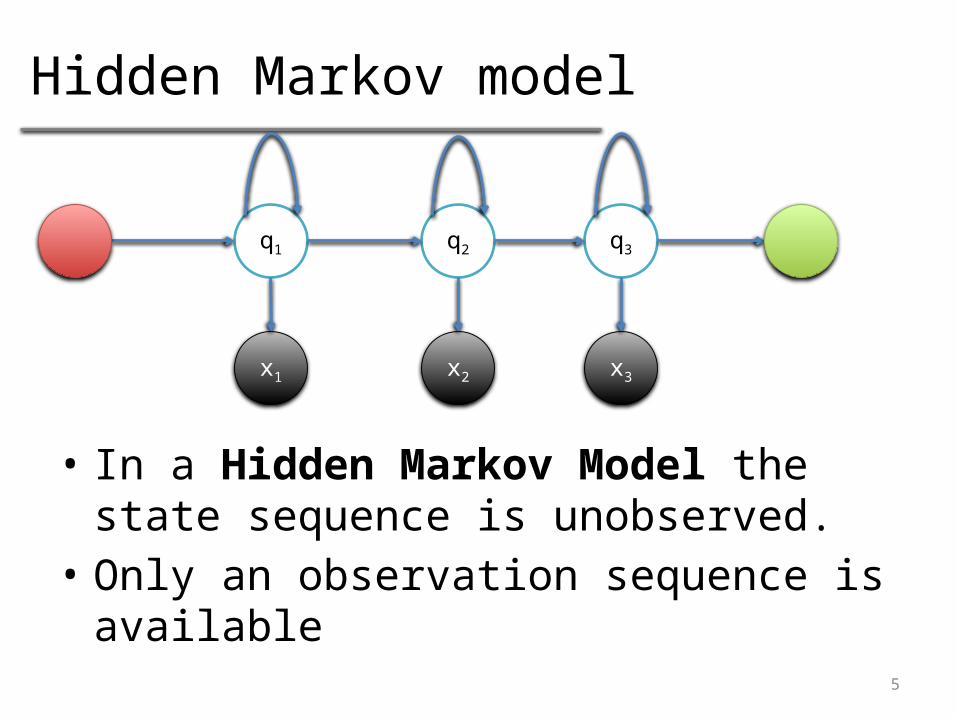
Hidden Markov model

• In a Hidden Markov Model the state sequence is unobserved.

• Only an observation sequence is available

q1 q2 q3

x1 x2 x3

6

Hidden Markov model

• Observations are MFCC vectors• States are phone labels• Each state (phone) has an associated

GMM modeling the MFCC likelihood

q1 q2 q3

x1 x2 x3

7

Forward-Backwards Algorithm

• HMMs are trained by collecting and distributing information from observations to states.

• The Forward-Backwards algorithm is a specific example of EM.

• In the HMM topology (variable relationship), the training converges in one forward pass, and a backwards pass.– hence the name

8

Forwards Backwards Algorithm

• Forwards-Step:– Collect up from the observations to the states– Collect from left state to right state.

• “Collect” – update parameters to correctly model the observations– Observation collection will give a distribution over states, given the initial

state– State collection will also give a distribution over states– the new q distribution will reflect the combination of these two

q1 q2 q3

x1 x2 x3

9

Forwards Backwards Algorithm

• Backwards-Step:– Distribute down to the observations from the states– Collect from left state to right state.

• “Distribute” – update parameters to correctly model the observations– Observation distribute updates the state-observation relationship– State distribution updates the state-state transition matrix

• Forward-backwards can be shown to converge in one pass.

q1 q2 q3

x1 x2 x3

10

Finite State Automata

• “Start” “Accept” States• Epsilon Transitions• Relationship to Regular Expressions• Operations on FSA

– Addition– Inversion– Node expansion– Determinization

• Weighted automata allow probabilities to be assigned to transitions

11

State transitions as FSA

/d/ /t//ey/ /ax/

/ae/ /dx/

12

Word FSA to phone FSA

/d/ /t//

ey//

ax/

/ae/ /dx/

MORE DATA

/m/ /ao/ /r/

13

Word FSA to phone FSA

/d/ /t//

ey//

ax/

/ae/ /dx/

/m/ /ao/ /r/

14

Decoding a Hidden Markov Model

• Decoding is finding the most likely state sequence.

• How many state sequences are there in a HMM with N observations and k states?

15

Viterbi Decoding

• Dynamic Programming can make this a lot faster.

• Idea: Any optimal sequence between x0 and xn must include the optimal sequence between xn and xn-1.– Based on the Markov Assumption.

16

Viterbi Decoding

• Probability of most likely state sequence

• Recovering the the optimal sequence involves storing pointers as decisions are made.

17

Example (from Wikipedia)states = ('Rainy', 'Sunny') observations = ('walk', 'shop', 'clean') start_probability = {'Rainy': 0.6, 'Sunny': 0.4} transition_probability = { 'Rainy' : {'Rainy': 0.7, 'Sunny': 0.3}, 'Sunny' : {'Rainy': 0.4, 'Sunny': 0.6},} emission_probability = { 'Rainy' : {'walk': 0.1, 'shop': 0.4, 'clean': 0.5}, 'Sunny' : {'walk': 0.6, 'shop': 0.3, 'clean': 0.1},}

What is the most likely state sequence?

18

HMM Topology for Training

• Rather than having one GMM per phone, it is common for acoustic models to represent each phone as 3 triphones

S1 S3S2 S4 S5

/r/

19

Flat Start

• In Flat Start training, GMM parameters are initialized to global means and variances.

• Viterbi is used to perform forced alignment between observations and phone sequence.– The phone sequence is derived from the

lexical transcription and pronunciation model

20

Forced Alignment

• Given a phone sequence and observations, assign each observation to a phone.

• Uses– Identifying which observation belong to

each phone label for later training– Getting time boundaries for phone or

word labels.

21

Flat Start

• In Flat Start training, GMM parameters are initialized to global means and variances.

• Viterbi is used to perform forced alignment between observations and phone sequence.– The phone sequence is derived from the

lexical transcription and pronunciation model

• After alignment, retrain Acoustic Models, and repeat.

22

What about silence?

• If there is no “silence” state, the silent frames will be assigned to either the /d/ or the /ax/

• This leads to worse acoustic models.• A solution: Explicit training of silence models, /sp/

– Allowing /sp/ transitions at word boundaries

/d/ /ey/ /dx/ /ax/ /d/ /ey/ /dx/ /ax/ /d/ /ey/ /dx/ /ax/

23

Next Class

• Pronunciation Modeling• Reading: J&M Chapter 2,

Section10.5.3, 11.1, 11.2