Servers, R and Wild Mice

Robert William DaviesFeb 5, 2014

Overview

• 1 - How to be a good server citizen• 2 – Some useful tricks in R (including ESS)• 3 – Data processing – my wildmice pipeline

1 - How to be a good server citizen

• Three basic things– CPU usage

• cat /proc/cpuinfo• top• htop

– RAM (memory) usage• top• htop

– Disk IO and space• iostat• df -h

Cat /proc/cpuinforwdavies@dense:~$ cat /proc/cpuinfo | head processor : 0vendor_id : AuthenticAMDcpu family : 21model : 2model name : AMD Opteron(tm) Processor 6344 stepping : 0microcode : 0x600081ccpu MHz : 1400.000cache size : 2048 KBphysical id : 0

rwdavies@dense:~$ cat /proc/cpuinfo | grep processor | wc -l48

Htop and top

48 cores

Load average – average over 1, 5, 15 minutes

RAM – 512GB total142 in use (rest free)

Swap is BADIdeal use – 0(in this case it is probably residual)

Memory can be in RAM or in swap

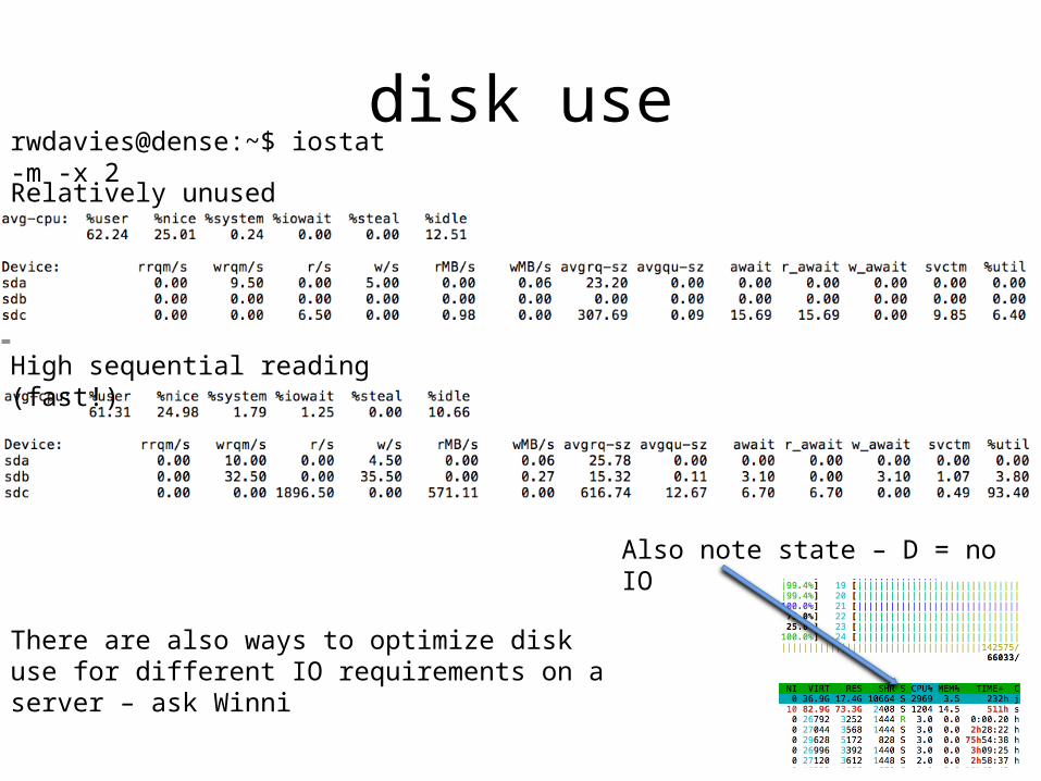
disk use

High sequential reading (fast!)

rwdavies@dense:~$ iostat -m -x 2

Relatively unused

Also note state – D = no IO

There are also ways to optimize disk use for different IO requirements on a server – ask Winni

Disk usageGet sizes of directories

Get available disk space

How to be a good server citizenTake away

• CPU usage– Different servers different philosophies– At minimum, try for load <=number of cores

• RAM– High memory jobs can take down a server very easily and will make

others mad at you – best to avoid• Disk IO

– For IO bound jobs you often get better combined throughput from running one or a few jobs than many in parallel

– Also don’t forget to try and avoid clogging up disks• P.s.

– A good server uptime is 100%

2 – Some useful tricks in R (including ESS)

• R is a commonly used programming language / statistical environment

• Pros– (Almost) everyone uses it– Very easy to use

• Cons– It’s slow– It can’t do X

• But! R can be faster, and it might be able to do X! Here I’ll show a few tricks

ESS (Emacs speaks statistics)

• Emacs is a general purpose text editor• Lots of programs exist for using R• There exists an extension to emacs called ESS

allowing you to use R within emacs• This allows you to analyze data on a server

very nicely using a split screen environment and keyboard shortcuts to run your code

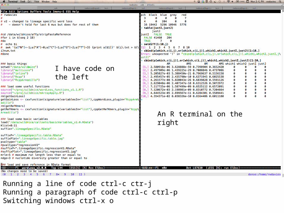
I have code on the left

An R terminal on the right

Running a line of code ctrl-c ctr-jRunning a paragraph of code ctrl-c ctrl-pSwitching windows ctrl-x o

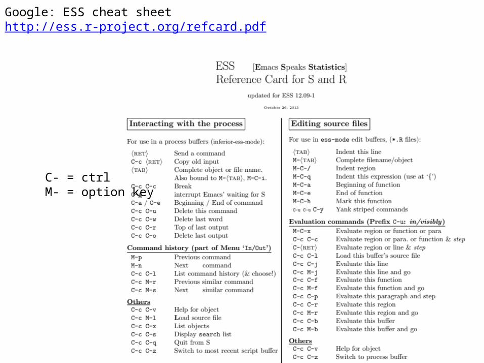
Google: ESS cheat sheethttp://ess.r-project.org/refcard.pdf

C- = ctrlM- = option key

R – mclapply

• lapply – apply a function to members of a list• mclapply – do it multicore!• Note there exists a spawning cost depending

on memory of current R job

Not 19X faster due to chromosome size differencesAlso I ran this on a 48 core server with a load of 40

/dev/shm

• (This might be an Ubuntu Linux thing?)• Not really an R thing but can be quite useful for R

multicore• /dev/shm uses RAM but operates like disk for

many input / output things• Example: You loop on 2,000 elements, each of

which generates an object of size 10Mb. You can pass that all back at once to R (very slow) or write to /dev/shm and read the files back in (faster)

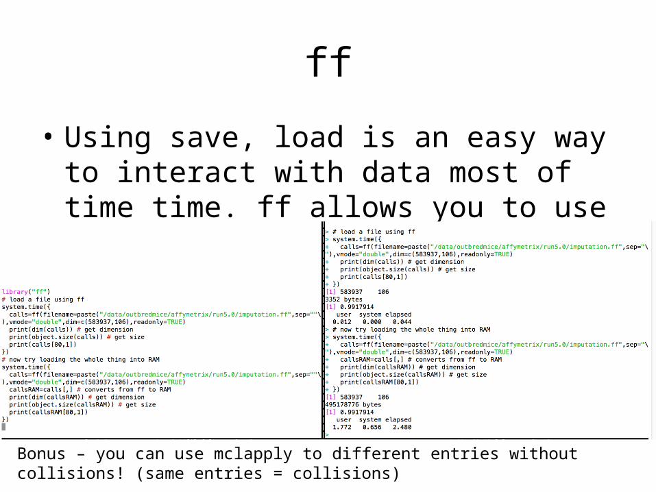
ff

• Using save, load is an easy way to interact with data most of time time. ff allows you to use variables like a pointer to RAM

Bonus – you can use mclapply to different entries without collisions! (same entries = collisions)

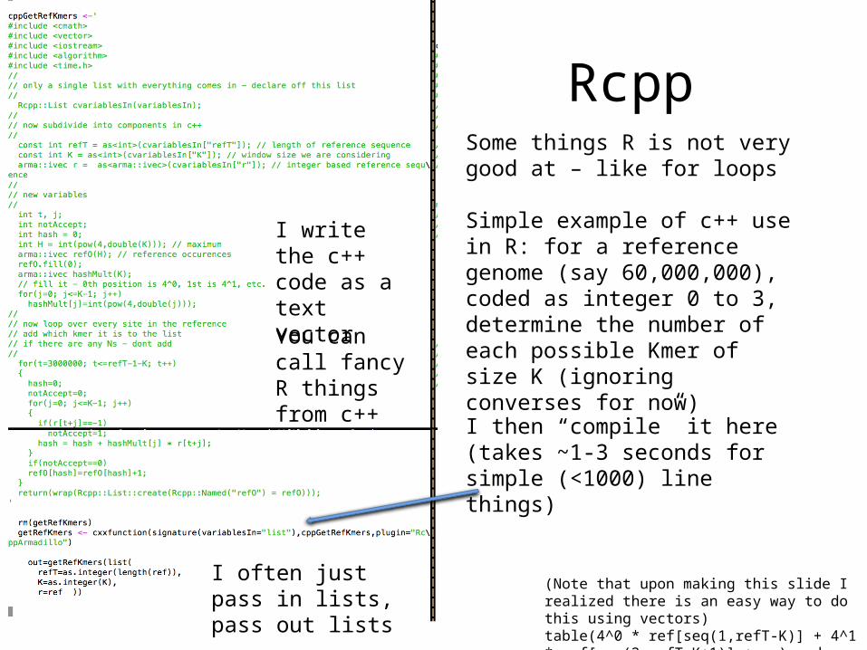
Rcpp

I write the c++ code as a text vector

I then “compile” it here (takes ~1-3 seconds for simple (<1000) line things)

Some things R is not very good at – like for loops

Simple example of c++ use in R: for a reference genome (say 60,000,000), coded as integer 0 to 3, determine the number of each possible Kmer of size K (ignoring converses for now)

(Note that upon making this slide I realized there is an easy way to do this using vectors)table(4^0 * ref[seq(1,refT-K)] + 4^1 * ref[seq(2,refT-K+1)] + … ) and adjusting for NAs

I often just pass in lists, pass out lists

You can call fancy R things from c++

Complicated example I actually use

• Want to do an EM HMM with 2000 subjects and up to 500,000 SNPs with 30 rounds of updating

• Using R – pretty fast, fairly memory efficient– Use Rcpp to make c++ forward backward code in R– for iteration from 1 to 30

• mclapply on 2000 subjects – Run using Rcpp code, write output to /dev/shm/

• Aggregate results from /dev/shm to get new parameters

– Write output (huge) to ff for easy downstream analysis

• A lot of people complain about R being slow but it’s really not that slow– Many packages such as Rcpp, ff, multicore, etc, let your code

run much faster– Also, vector or matrix based R is pretty much as fast as

anything• If 1 month after starting to use R you are still copying

and pasting, stop what you’re doing and take a day to learn ESS or something similar– If you don’t use R often you can probably ignore this– (P.s. I copied and pasted for 2 or 3 years before using ESS)

2 – Some useful tricks in R (including ESS) – Take away

3 – Data processing – my wildmice pipeline

• We have data on 69 mice• Primary goals of this study– Recombination• Build rate maps for different subspecies• Find motifs

– Population genetics• Relatedness, history, variation• Admixture

N=1 - 40X - WDIS

N=1 - 40X - WDIS

N=1 - 40X – WDIS = Wild derived inbred strain

N=1 - 40X - WDIS

N=1 - 40X - WDIS

N=1 - 40X - WDIS

N=20 - 10X - Wild

N=10 - 30X - Wild

N=20 - 10X - Wild

N=13- 40X – Lab strains

M. m. Domesticus

M. m. Castaneus

M. m. musculus

bwa aln –q 10Stampy –bamkeepgoodreadsAdd Read group infoMerge into library level BAM using picard MergeSamFiles

69 analysis ready BAMS!

Picard markDuplicatesMerge into sample level BAM

Use GATK RealignerTargetCreator on each populationRealign using GATK IndelRealigner per BAM

Use GATK UnifedGenotyper on each population to create a list of putative variant sites.GATK BaseRecalibrator to generate recalibration tables per mouseGaTK PrintReads to apply recalibration

6 pops – 20 French, 20 Taiwan, 10 Indian, 17 Strains, 1 Fam, 1 Caroli

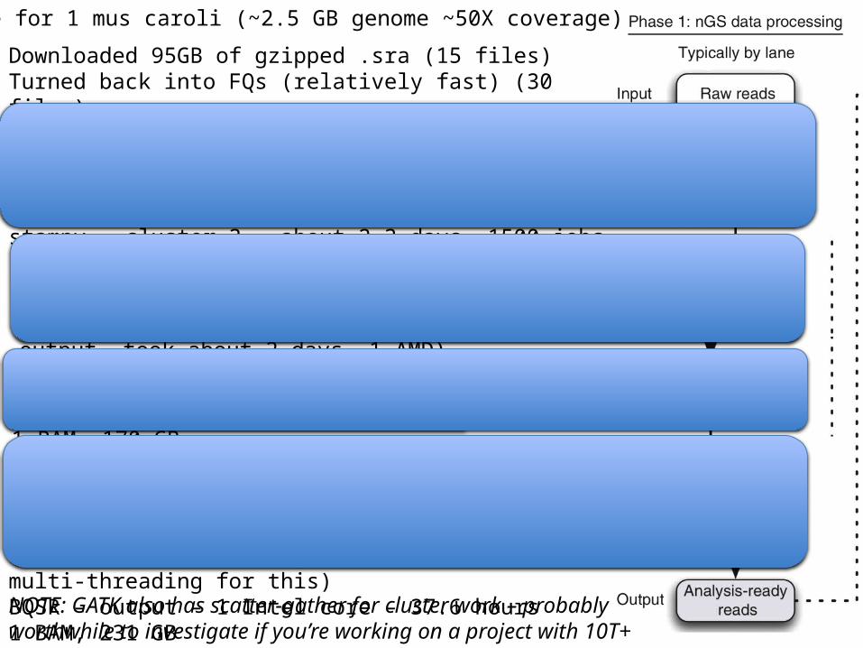
Downloaded 95GB of gzipped .sra (15 files)Turned back into FQs (relatively fast) (30 files)

bwa – about 2 days at 40 AMD cores (86 GB output, 30 files)Merged 30 -> 15 files (215 GB)stampy – cluster 3 – about 2-3 days, 1500 jobs (293 GB output, 1500 files)

Example for 1 mus caroli (~2.5 GB genome ~50X coverage)

Merge stampy jobs together, turn into BAMs (220 GB 15 files)Merge library BAMs together, then remove duplicates per library, then merge and sort into final BAM (1 output, took about 2 days, 1 AMD)1BAM, 170 GB

NOTE: GATK also has scatter-gather for cluster work – probably worthwhile to investigate if you’re working on a project with 10T+ data

Indel realignment – find intervals – 16 Intel cores, fast (30 mins)Apply realignment – 1 intel core – slower 1 BAM, 170 GB

BQSR – call putative set of variants – 16 intel cores – (<2 hours)BQSR – generate recalibration tables – 16 intel cores – 10.2 hours(note – used relatively new GATK which allows multi-threading for this)BQSR – output – 1 Intel core – 37.6 hours1 BAM, 231 GB

Wildmice – calling variants

• We made two sets of callsets– 3 population specific (Indian, French, Taiwanese),

principally for estimating recombination rate• FP susceptible – prioritize low error at the expense of

sensitivity

– Combined – for pop gen• We used the GATK to call variants and VQSR to

filter

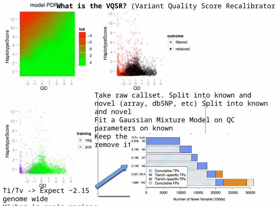
Take raw callset. Split into known and novel (array, dbSNP, etc) Split into known and novelFit a Gaussian Mixture Model on QC parameters on knownKeep the novel that’s close to the GMM, remove if far away

What is the VQSR? (Variant Quality Score Recalibrator)

Ti/Tv -> Expect ~2.15 genome wideHigher in genic regions

Population Training Sensitivity HetsInHomE chrXHetE nSNPs TiTv arrayCon arraySen

French Array Filtered 95 0.64 1.97 12,957,830 2.20 99.08 94.02

French Array Filtered 97 0.72 2.28 14,606,149 2.19 99.07 96.01

French Array Filtered 99 1.12 3.62 17,353,264 2.16 99.06 98.09

French Array Not Filt 95 2.06 5.82 18,071,593 2.14 99.07 96.58

French Array Not Filt 97 2.97 8.24 19,369,816 2.10 99.07 98.01

French Array Not Filt 99 6.11 15.73 22,008,978 2.01 99.06 99.20French 17 Strains 95 1.29 3.89 16,805,717 2.14 99.07 93.49French 17 Strains 97 2.20 6.52 18,547,713 2.11 99.07 96.49French 17 Strains 99 4.19 11.63 20,843,679 2.04 99.06 98.62French Hard Filters NA 5.36 16.37 19,805,592 2.06 99.09 96.96

Sensitivity – You set this – How much of your training set do you want to recoverHetsInHomE – Look at homozygous regions in the mouse – how many hets do you seechrXHetE – Look at chromosome X in males – how many hets do you seenSNPs – number of SNPsTiTv – transition transversion ratio – expect ~2.15 for real, 0.5 for FParrayCon – Concordance with array genotypesarraySen – Sensitivity for polymorphic array sites

We chose a dataset for recombination rate estimation with low error rate but still a good number of SNPs

Notes – VQSR sensitivity not always “calibrated” -

It’s a good idea to benchmark your callsets and decide on the one with the parameters that suit the needs of your project (like sensitivity (finding everything) vs specificity (being right))

Population Training Sensitivity HetsInHomE chrXHetE nSNPs TiTv arrayCon arraySen

Taiwan Array Not Filt 95 2.05 11.20 36,344,063 2.12 NA NA

Taiwan Array Not Filt 97 2.87 14.67 39,183,932 2.10 NA NA

Taiwan Array Not Filt 99 6.34 25.57 42,864,322 2.05 NA NATaiwan 17 Strains 95 1.83 10.32 29,748,456 2.11 NA NATaiwan 17 Strains 97 2.16 11.20 34,112,325 2.11 NA NATaiwan 17 Strains 99 3.66 15.80 39,549,666 2.08 NA NATaiwan Hard Filters NA 6.11 19.44 33,692,857 2.04 NA NA

Indian Array Not Filt 95 1.11 1.80 66,190,390 2.18 NA NA

Indian Array Not Filt 97 1.59 2.57 71,134,757 2.16 NA NA

Indian Array Not Filt 99 3.70 5.56 78,220,348 2.11 NA NAIndian 17 Strains 95 0.67 1.16 57,674,209 2.18 NA NAIndian 17 Strains 97 1.09 1.63 65,981,654 2.17 NA NAIndian 17 Strains 99 2.63 3.31 75,103,886 2.13 NA NA

Indian Hard Filters NA 5.41 72.61 78,487,616 2.10 NA NA

All Array Not Filt 95 1.90 8.95 140,827,810 2.04 99.07 96.74

All Array Not Filt 97 2.38 13.99 160,447,255 2.03 99.07 98.20

All Array Not Filt 99 4.52 22.73 184,977,157 1.99 99.06 99.36

Some of the datasets are extremely bigCombined datasets allow us to better evaluate differences between populations

Notes – VQSR sensitivity not always “calibrated” – Note: Be VERY skeptical of the work of others wrt sensitivity, specificity, that depends on NGS. Different filtering on different datasets can often explain alot

Huge Taiwan and French bottleneck, India OK

Homozygosity = red

French and Taiwanese very inbred, not so for the Indian mice

Taiwan

France

India

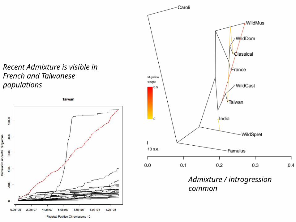
Admixture / introgression common

Recent Admixture is visible in French and Taiwanese populations

French hotspots are cold in Taiwan and vice-versa

Our Domesticus hotspots are enriched in an already known Domesticus motif

Broad scale correlation is conserved between subspecies, like in humans vs chimps

Conclusions

• 1 – Don’t crash the server• 2 – There are tricks to make R faster• 3 – Sequencing data is big, slow and unwieldy.

But it can tell us a lot

Acknowledgements

• Simon Myers – supervisor• Jonathan Flint, Richard Mott – collaborators• Oliver Venn – Recombination work for wild mice• Kiran Garimella – GATK guru• Cai Na – Pre-processing pipeline• Winni Kretzschmar – ESS, and many other things

he does I copy• Amelie Baud, Binnaz Yalcin, Xiangchao Gan and

many others for the wild mice