session 18 estimating net survival { past and present · session 18 estimating net survival { past...

Session 18

Estimating net survival – past and present

Paul W Dickman1 and Paul C Lambert1,2

1Department of Medical Epidemiology and Biostatistics,Karolinska Institutet, Stockholm, Sweden

2Department of Health Sciences,University of Leicester, UK

Cancer survival: principles, methods and applicationsLSHTM

July 2014

Choose a measure and then choose an estimator

Crude survival (real world probabilities) [measure]

Choice of estimators in either cause-specific or relative survivalsetting. [See session 19]

Net survival (hypothetical world probabilities) [measure]Cause-specific setting

Censor the survival times of those who die of other causes andapply standard estimators (e.g., Kaplan-Meier).

Relative survival setting (Berkson 1942 [1])

Ederer I (1961 [2])Ederer II (1959 [3])Hakulinen (1982 [4])Pohar Perme (2012 [5])Model-based (Esteve et al. 1990 [6] plus others)

Dickman and Lambert Population-Based Cancer Survival LSHTM, June 2014 2

‘Net survival’ is not a new concept

The distinction between net probabilities and crude probabilitieshas a long history in the theory of competing risks.

Not new in the field of population-based cancer survival.Jacques Esteve and colleagues (1990) [6] were very explicit thatnet survival is a theoretical measure that can be estimated byeither cause-specific survival or relative survival.

‘Although this is hardly explicit in [Ederer et al. 1961 [2]], theintention of the originators of this concept was to estimate netsurvival’ [page 531]


A major breakthrough; Pohar Perme et al. 2012 [5]

Although the concept of net survival is not new, we only recentlyfully understood what it is (and what it isn’t).

Pohar Perme et al. 2012 [5] described net survival (the measure)and the various estimators in a formal framework.

They showed that net survival is

net survival =1

n

n∑

i=1

Si(t)

S∗i (t)

.

Which is not the same as

relative survival =1n

∑ni=1 Si(t)

1n

∑ni=1 S

∗i (t)

.


Comments

The Pohar Perme method does not estimate relative survival(the marginal observed divided by the marginal expectedsurvival). It does, however, estimate net survival in a relativesurvival setting (rather than a cause-specific setting). Here, Ibelieve, Maja and I agree.

Among the estimators in a relative survival setting, Pohar Permeis the only one that is an unbiased estimator of net survival.This is indisputable.

Where we disagree, is that I view all of the relative survivalbased estimators as estimators of net survival.

Bias in Ederer II is usually small in practice. [Here we agree]


Why would one use a biased estimator (even small

bias) when an unbiased alternative exists?

I’m not crazy! I am a great fan of the Pohar Perme estimator.

However, I don’t think the Ederer II and model-based estimatorsare as biased as some would have you believe.

My main message has been ‘previous estimates made withEderer II as not necessarily greatly biased’.

My other message has been that, if moving to the new estimatoris a non-trivial exercise (e.g., need to introduce new software)then one should be aware that the benefit (reduced bias) is quitesmall’.

If you want to do more than nonparametric estimation of netsurvival then modelling has advantages.


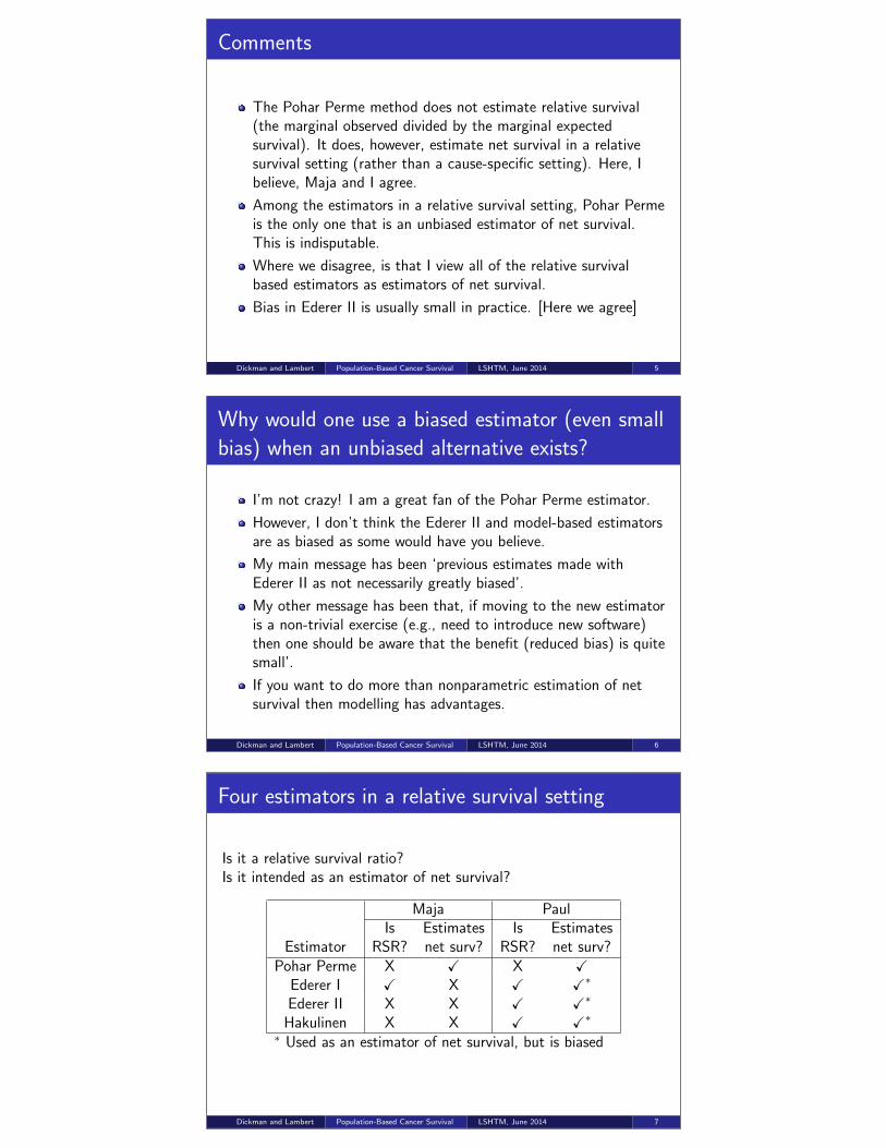
Four estimators in a relative survival setting

Is it a relative survival ratio?Is it intended as an estimator of net survival?

Maja PaulIs Estimates Is Estimates

Estimator RSR? net surv? RSR? net surv?Pohar Perme X X X X

Ederer I X X X X∗

Ederer II X X X X∗

Hakulinen X X X X∗

∗ Used as an estimator of net survival, but is biased


Quotes from recent work: Roche et al [7]

In estimating net survival, cancer registries should abandonall classical methods and adopt the new Pohar-Permeestimator.

Unfortunately, due to inherent biases, most of the statisticalmethods used to estimate net survival are quite inaccurate.”

Great errors may occur ...

We see no reason to favor any classically used method suchas Ederer I, Hakulinen, Ederer II or the univariableexcess-rate regression models because, unlike the PPE, theyare all biased”

Similar views in other papers [7, 8, 9, 10].


Our response [11]

“... we believe Roche et al. misrepresent the bias in the preferredclassical methods in a manner that may unduly cause alarm.”

“... it would be a great pity if the scientific community dismissedmethodologically sound and important research because ofRoche and coworker’s claims of “great errors.”

“... the comparisons by Roche et al. are not objective; theygrossly overstate the magnitude of the bias in the Ederer IImethod in a manner that could mislead and alarm the researchcommunity.”

“The approach used by Roche et al. to calculate the “bias withthe classical methods” is fundamentally flawed.”

“Researchers should also be aware that the lack of bias in thePP estimator comes at a price of higher variance.”


A difference in estimates is not bias

0.2

0.4

0.6

0.8

1.0

Rel

ativ

e S

urvi

val

0 5 10Years since diagnosis

Ederer IIPohar Perme

Colon Cancer: Males: Age 75+: Year 1985-94


Relative survival is an estimator of net survival

We view relative survival as an approach to estimating netsurvival.

Pohar Perme [5] showed that relative survival, as it is usuallycalculated, is a biased estimator of net survival. This isindisputable.

This has lead to some people viewing relative survival as aseparate and distinct quantity to net survival. We disagree.

Relative survival is a method for estimating net survival. It isbiased, but the bias in practice is so small (Ederer II or modellingapproach) that it can be ignored (see later).


Relative survival was designed

to estimate net survival

The concept of relative survival, the ratio of observed toexpected survival, was introduced by Berkson in 1942 [1],although he did not use the term ‘relative survival’.

He proposed relative survival as an estimator for ‘the survival sofar as cancer is concerned’ [1], the concept that is today knownas net survival.

Although the term ‘net surival’ was not used in the earlyliterature, Berkson and Ederer viewed both cause-specificsurvival and relative survival as estimators of net survival, a viewthat we share.


Definition of relative survival

In their seminal article from 1961 [2], Ederer and colleaguesdefined the ‘relative survival rate’ as‘the ratio of the observed survival rate in a group of patients,during a specified interval, to the expected survival rate. Theexpected survival rate is that of a group similar to the patientgroup in such characteristics as age, sex, and race, but free ofthe specific disease under study’. [their emphasis]

Relative survival is a ratio rather than a rate, and observed andexpected survival are proportions rather than rates, but weotherwise use this same definition.

We define relative survival as the the ratio of the all-causesurvival of the patients to the (all-cause) survival that would beexpected in the absence of the specific disease under study.


Choice of approach for calculating relative survival

Each of the following approaches provide reasonable estimates of5-year net survival for most applications:

1 Model-based2 Ederer II (age standardised)3 Pohar Perme

We can show, in extreme scenarios, that the Pohar Permemethod is highly variable but this is not a concern for mostpractical applications.

Ederer II is theoretically biased, but the bias is so small that itdoesn’t matter in practice (provided one age-standardises).

We prefer model-based estimation, but any of the estimators canbe used.


Choice of approach for estimating net survival

We view the Pohar Perme estimator as an estimator of netsurvival in a relative survival framework; it doesn’t estimaterelative survival (the marginal observed divided by the marginalexpected) but it uses a relative survival, rather than acause-specific, approach.

The Pohar Perme method estimates the following quantity

R s(t) =1

n

n∑

i=1

Si(t)

S∗i (t)

.

It can be interpreted as the marginal net survival under the sametwo assumptions (presented in the next section) that arerequired to interpret relative survival as net survival.


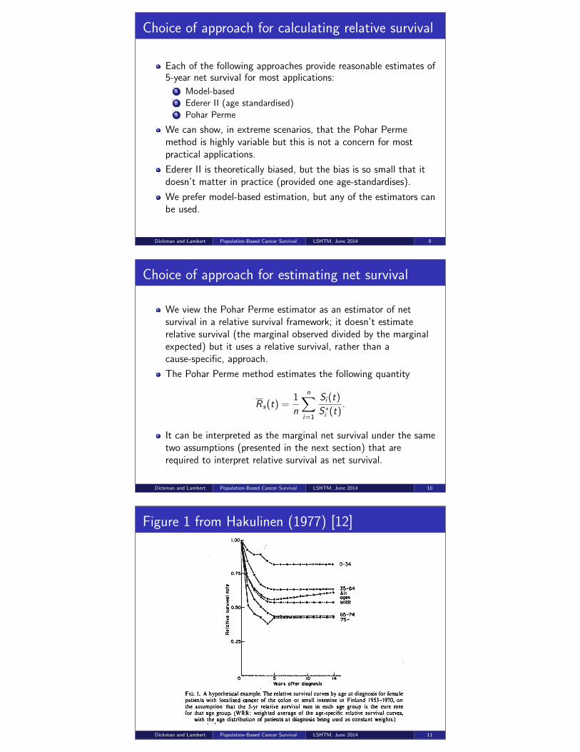
Figure 1 from Hakulinen (1977) [12]


The ‘Hakulinen method’ (1982) [4]


Timo Hakulinen changes his recommendation [13]

Choosing the relative survival method for cancer survivalestimation

Timo Hakulinen a,*, Karri Seppa a,b, Paul C. Lambert c,d

a Finnish Cancer Registry, Institute for Statistical and Epidemiological Cancer Research, Pieni Roobertinkatu 9, FI-00130 Helsinki, Finlandb Department of Mathematical Sciences, University of Oulu, Oulu, Finlandc Department of Health Sciences, Centre for Biostatistics and Genetic Epidemiology, University of Leicester, 2nd Floor, Adrian Building,

University Road, Leicester LE1 7RH, UKd Medical Epidemiology and Biostatistics, Karolinska Institutet, Stockholm, Sweden

A R T I C L E I N F O

Article history:

Received 22 November 2010

Received in revised form 7 March

2011

Accepted 9 March 2011

Available online 4 May 2011

Keywords:

Epidemiologic methods

Models

Neoplasms

Prognosis

Survival

Age standardisation

A B S T R A C T

Background: The methods on how to calculate cumulative relative survival have been

ambiguous and have given differences in empirical results.

Methods: The gold standard for the cumulative relative survival ratio is the weighted aver-

age of age-specific cumulative relative survival ratios, with weights proportional to num-

bers of patients at diagnosis. Mathematics and representative empirical materials from

the population-based Finnish Cancer Registry were studied for the different relative sur-

vival methods and compared with the gold standard.

Results: The theoretical and empirical results show a good agreement between the method

suggested in 1959 by Ederer and Heise (the so-called Ederer II method) and the gold stan-

dard. This result is in part due the fact that as follow-up time increases the conditional

(annual) relative survival ratios become increasingly more independent of age. Moreover,

the dependence between the excess mortality due to cancer and the baseline general mor-

tality does not introduce an important enough selection in practice to cause a notable bias.

Conclusion: The use of the method by Ederer and Heise, multiplication of the annual rela-

tive survival ratios, instead of direct standardisation, should be considered in future appli-

cations. This would be particularly important for the long-term follow-up when age-

specific relative survival is not available in the oldest age categories.

� 2011 Elsevier Ltd. All rights reserved.

1. Introduction

Relative survival has been used by the world’s population-

based cancer registries for 60 years to give estimates of pa-

tient survival as far as their cancer is concerned, in the ab-

sence of other causes of death.1,2 No cause-of-death

information is needed as the mortality from other causes of

death (expected mortality) is estimated from general popula-

tion life tables.

Two ways of estimating the cumulative relative survival ra-

tios were proposed by Ederer et al.: multiplication of the an-

nual conditional relative survival ratios3 and dividing the

cumulative observed survival proportion by the cumulative

expected proportion.4 The results given by these two meth-

ods, often called the Ederer II and I methods, respectively, dif-

fer markedly, particularly when the length of follow-up

exceeds ten years.5,6 It has been shown that the results given

by the Ederer I method converge with prolonged follow-up

0959-8049/$ - see front matter � 2011 Elsevier Ltd. All rights reserved.doi:10.1016/j.ejca.2011.03.011

* Corresponding author: Tel.: +358 9 135 331; fax: +358 9 135 5378.E-mail address: [email protected] (T. Hakulinen).

E U R O P E A N J O U R N A L O F C A N C E R 4 7 ( 2 0 1 1 ) 2 2 0 2 – 2 2 1 0

avai lab le at www.sc iencedi rec t .com

journal homepage: www.ejconl ine.com

Choosing the relative survival method for cancer survivalestimation

Timo Hakulinen a,*, Karri Seppa a,b, Paul C. Lambert c,d

a Finnish Cancer Registry, Institute for Statistical and Epidemiological Cancer Research, Pieni Roobertinkatu 9, FI-00130 Helsinki, Finlandb Department of Mathematical Sciences, University of Oulu, Oulu, Finlandc Department of Health Sciences, Centre for Biostatistics and Genetic Epidemiology, University of Leicester, 2nd Floor, Adrian Building,

University Road, Leicester LE1 7RH, UKd Medical Epidemiology and Biostatistics, Karolinska Institutet, Stockholm, Sweden

A R T I C L E I N F O

Article history:

Received 22 November 2010

Received in revised form 7 March

2011

Accepted 9 March 2011

Available online 4 May 2011

Keywords:

Epidemiologic methods

Models

Neoplasms

Prognosis

Survival

Age standardisation

A B S T R A C T

Background: The methods on how to calculate cumulative relative survival have been

ambiguous and have given differences in empirical results.

Methods: The gold standard for the cumulative relative survival ratio is the weighted aver-

age of age-specific cumulative relative survival ratios, with weights proportional to num-

bers of patients at diagnosis. Mathematics and representative empirical materials from

the population-based Finnish Cancer Registry were studied for the different relative sur-

vival methods and compared with the gold standard.

Results: The theoretical and empirical results show a good agreement between the method

suggested in 1959 by Ederer and Heise (the so-called Ederer II method) and the gold stan-

dard. This result is in part due the fact that as follow-up time increases the conditional

(annual) relative survival ratios become increasingly more independent of age. Moreover,

the dependence between the excess mortality due to cancer and the baseline general mor-

tality does not introduce an important enough selection in practice to cause a notable bias.

Conclusion: The use of the method by Ederer and Heise, multiplication of the annual rela-

tive survival ratios, instead of direct standardisation, should be considered in future appli-

cations. This would be particularly important for the long-term follow-up when age-

specific relative survival is not available in the oldest age categories.

� 2011 Elsevier Ltd. All rights reserved.

1. Introduction

Relative survival has been used by the world’s population-

based cancer registries for 60 years to give estimates of pa-

tient survival as far as their cancer is concerned, in the ab-

sence of other causes of death.1,2 No cause-of-death

information is needed as the mortality from other causes of

death (expected mortality) is estimated from general popula-

tion life tables.

Two ways of estimating the cumulative relative survival ra-

tios were proposed by Ederer et al.: multiplication of the an-

nual conditional relative survival ratios3 and dividing the

cumulative observed survival proportion by the cumulative

expected proportion.4 The results given by these two meth-

ods, often called the Ederer II and I methods, respectively, dif-

fer markedly, particularly when the length of follow-up

exceeds ten years.5,6 It has been shown that the results given

by the Ederer I method converge with prolonged follow-up

0959-8049/$ - see front matter � 2011 Elsevier Ltd. All rights reserved.doi:10.1016/j.ejca.2011.03.011

* Corresponding author: Tel.: +358 9 135 331; fax: +358 9 135 5378.E-mail address: [email protected] (T. Hakulinen).

E U R O P E A N J O U R N A L O F C A N C E R 4 7 ( 2 0 1 1 ) 2 2 0 2 – 2 2 1 0

avai lab le at www.sc iencedi rec t .com

journal homepage: www.ejconl ine.com


Informative right-censoring

To make it possible for statistical analysis we make the crucialassumption that, conditional on the values of any explanatoryvariables, censoring is unrelated to future prognosis.

The statistical methods used for survival analysis assume thatthe prognosis for an individual censored at time t will be nodifferent from those individuals who were alive at time t andwere under follow-up past time t.

One way to think of this is that, conditional on the values of anyexplanatory variables, the individuals censored at time t shouldbe a random sample of the individuals at risk at time t.

This is known as noninformative censoring. Under thisassumption, there is no need to distinguish between the differentreasons for right-censoring.


Informative right-censoring 2

When withdrawal from follow-up is associated with prognosis,this is known as informative censoring and standard methods ofanalysis will result in biased estimates.

Common methods for controlling for informative censoring are tostratify or condition on those explanatory factors on whichcensoring depends.

Determining whether or not censoring is informative is not astatistical issue — it must be made based on subject matterknowledge.


Cervical cancer in New Zealand 1994 – 2001

Life table estimates of patient survival

Women diagnosed 1994 - 2001 with follow-up to the end of 2002

Interval-

Number Effective specific Cumulative

at risk Deaths Censored number observed observed

I N D W at risk survival survival

1 1559 209 0 1559.0 0.86594 0.86594

2 1350 125 177 1261.5 0.90091 0.78014

3 1048 58 172 962.0 0.93971 0.73310

4 818 32 155 740.5 0.95679 0.70142

5 631 23 148 557.0 0.95871 0.67246

6 460 10 130 395.0 0.97468 0.65543

7 320 5 129 255.5 0.98043 0.64261

8 186 3 134 119.0 0.97479 0.62641

9 49 1 48 25.0 0.96000 0.60135


Cervical cancer in New Zealand 1994 – 2001

Life table estimates of patient survival

Women diagnosed 1994 - 2001 with follow-up to the end of 2002

Interval- Interval-

Effective specific specific Cumulative Cumulative Cumulative

number observed relative observed expected relative

I N D W at risk survival survival survival survival survival

1 1559 209 0 1559.0 0.86594 0.87472 0.86594 0.98996 0.87472

2 1350 125 177 1261.5 0.90091 0.90829 0.78014 0.98192 0.79450

3 1048 58 172 962.0 0.93971 0.94772 0.73310 0.97362 0.75296

4 818 32 155 740.5 0.95679 0.96459 0.70142 0.96574 0.72630

5 631 23 148 557.0 0.95871 0.96679 0.67246 0.95766 0.70218

6 460 10 130 395.0 0.97468 0.98284 0.65543 0.94972 0.69013

7 320 5 129 255.5 0.98043 0.98848 0.64261 0.94198 0.68219

8 186 3 134 119.0 0.97479 0.98405 0.62641 0.93312 0.67130

9 49 1 48 25.0 0.96000 0.97508 0.60135 0.91869 0.65457


Necessary assumptions for relative survival to

estimate net survival

For RSR to estimate net survival, we need1 appropriate population life tables; and2 independence (conditional on covariates) of cancer and

non-cancer mortality.

What do we mean by ‘independence’ in this context? We meanthat there are no factors associated with both cancer andnon-cancer mortality other than those factors that are adjustedfor in both the analysis and in the population mortality file.

The Pohar Perme estimator addresses point 2 in anon-parametric setting, but assumption 1 must still be assessed(for all RSR-based estimators).


Necessary assumptions for cause-specific survival

to estimate net survival

For cause-specific survival to estimate net survival, we need1 accurate cause of death information; and2 independence (conditional on covariates) of cancer and

non-cancer mortality.

What do we mean by ‘independence’ in this context? We meanthat there are no factors associated with both cancer andnon-cancer mortality other than those factors for which we haveadjusted in the model.


Assumptions required for estimating crude

probabilities of death

To estimate crude probabilities of death in a cause-specificsetting, we do not require the independence assumption (we onlyrequire correct classification of cause of death).

Similarly, the independence assumption is not required toestimate crude probabilities of death in a relative survivalframework (we only require appropriate population life tables).


Summary: Ederer I, Ederer II, and Hakulinen

Expected survival can be thought of as being calculated for acohort of patients from the general population matched by age,sex, and period. The methods differ regarding how long eachindividual is considered to be ‘at risk’ for the purpose ofestimating expected survival.Ederer I: the matched individuals are considered to be at riskindefinitely (even beyond the closing date of the study). Thetime at which a cancer patient dies or is censored has no effecton the expected survival.Ederer II: the matched individuals are considered to be at riskuntil the corresponding cancer patient dies or is censored.Hakulinen: if the survival time of a cancer patient is censoredthen so is the survival time of the matched individual. However,if a cancer patient dies the matched individual is assumed to be‘at risk’ until the closing date of the study.


Illustration of expected survival estimation


The Pohar Perme estimator

First presented in 2011, published in 2012 [5].

Pohar Perme et al. illustrate that existing relative survival-basedestimators do not exactly estimate marginal net survival, andpresented a new unbiased estimator.

The new approach estimates net survival as internallyage-standardized relative survival, but without the need toperform separate calculations for each age strata.

The method addresses the specific scenario where we wish toestimate net survival, non-parametrically, for a single cohort(i.e., all ages). Pohar Perme et al. remark in their paper that amodel-based approach is also possible.


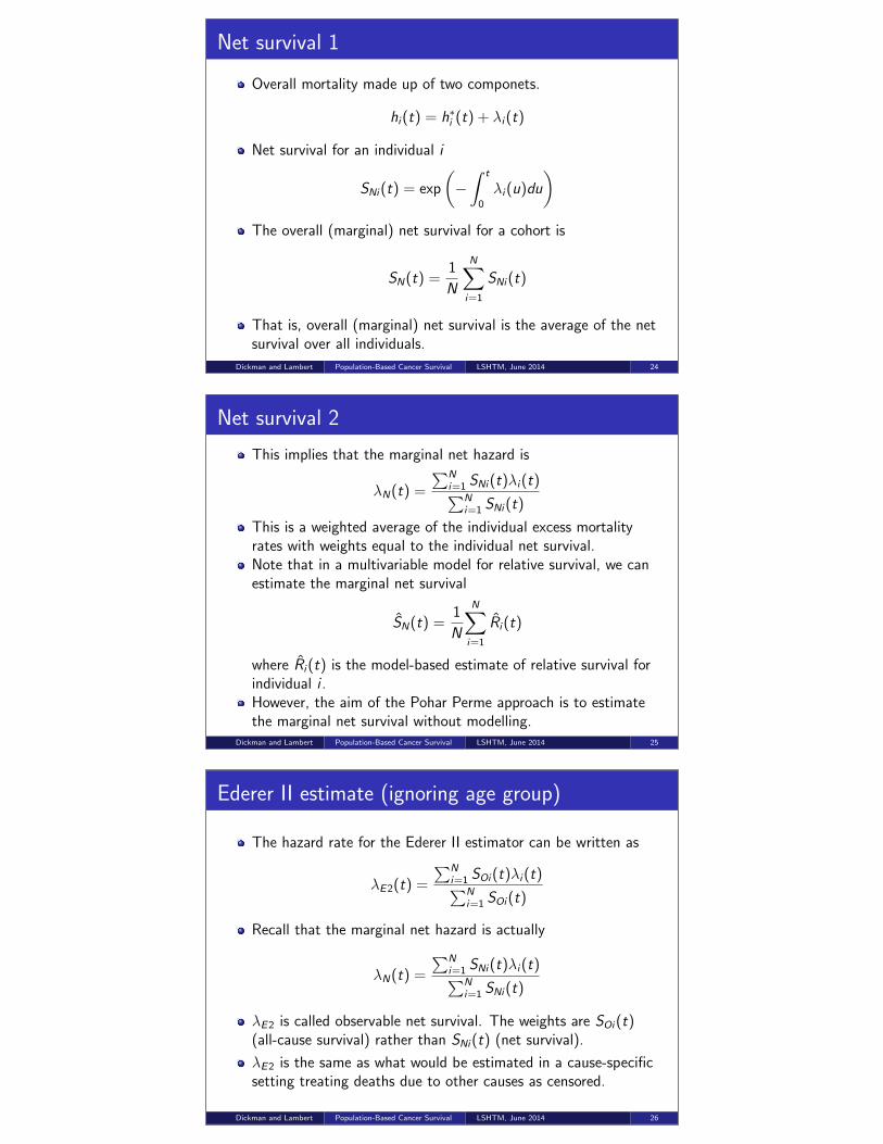
Net survival 1

Overall mortality made up of two componets.

hi(t) = h∗i (t) + λi(t)

Net survival for an individual i

SNi(t) = exp

(−∫ t

0

λi(u)du

)

The overall (marginal) net survival for a cohort is

SN(t) =1

N

N∑

i=1

SNi(t)

That is, overall (marginal) net survival is the average of the netsurvival over all individuals.


Net survival 2

This implies that the marginal net hazard is

λN(t) =

∑Ni=1 SNi(t)λi(t)∑N

i=1 SNi(t)

This is a weighted average of the individual excess mortalityrates with weights equal to the individual net survival.Note that in a multivariable model for relative survival, we canestimate the marginal net survival

SN(t) =1

N

N∑

i=1

Ri(t)

where Ri(t) is the model-based estimate of relative survival forindividual i .However, the aim of the Pohar Perme approach is to estimatethe marginal net survival without modelling.


Ederer II estimate (ignoring age group)

The hazard rate for the Ederer II estimator can be written as

λE2(t) =

∑Ni=1 SOi(t)λi(t)∑N

i=1 SOi(t)

Recall that the marginal net hazard is actually

λN(t) =

∑Ni=1 SNi(t)λi(t)∑N

i=1 SNi(t)

λE2 is called observable net survival. The weights are SOi(t)(all-cause survival) rather than SNi(t) (net survival).

λE2 is the same as what would be estimated in a cause-specificsetting treating deaths due to other causes as censored.


Ederer I/Hakulinen estimates (ignoring age group)

Ederer II estimator can also be written,

λE2(t) = λO(t) −∑N

i=1 SOi(t)h∗i (t)∑Ni=1 SOi(t)

The hazard rate for the Ederer I estimate can be written as

λE1(t) = λO(t) −∑N

i=1 S∗i (t)h∗i (t)∑N

i=1 S∗i (t)

Hakulinen is the same under non-informative censoring.

Thus the current estimators (Ederer I and II and Hakulinen) donot exactly estimate net survival.


Summary of current estimators

When net survival is equal over ages (and sex etc.) then thedifferent estimators give identical estimates.

When expected survival is the same for all subjects, the differentestimators give identical estimates.

This is why we see less variation between methods whenestimating within age groups.

This is why there is less variation between the differentestimators of age-standardized estimates.


The New Estimator (adapted to discrete time)

The estimate of net survival is in a hypothetical world.

To be at risk at time t, an individual has,

not died of their cancer.not died of other causes.

Compared to the hypothetical world,

The number at risk is too small (because people die due tocauses other than cancer).The number of events (deaths due to cancer) is too small.

Solution: weight by inverse of expected survival.

Pohar Perme estimates in continuous time. Needs to be adaptedto discrete time.


The New Estimator

k - Interval lengthwij - Weight for i th subject in j th interval.dij - Event indicator for i th subject in j th interval.d∗ij - Expected deaths for i th subject in j th interval (d∗

ij = h∗ijyij).yij - Time at risk for i th subject in j th interval.

Estimate cumulative weighted excess hazard

Hwj =∑

j

k(∑

i wijdij −∑

wijd∗ij )∑

wijyij

Weights are the inverse of expected survival and vary as afunction of follow-up time.

The weights have the effect of increasing the sample still at riskto account for the expected proportion of patients lost due tomortality due to other causes.


Some comments on Pohar Perme

Provides an internally age standardized estimate of relativesurvival without the need to estimate relative survival separatelyby age group.

Strictly, the estimate is also standardized over other variables inthe population mortality file (usually calendar year and sex).

If comparing net survival between groups, the Pohar Permeestimate will not account for different age distributions in thedifferent groups. Still need to externally age standardize.

The method is designed for continuous time and is unbiased forcontinuous time. Properties unclear when we have discrete time.


Comparison of approaches (ignoring age group)

0.0

0.2

0.4

0.6

0.8

1.0

Rel

ativ

e S

urvi

val

0 5 10 15 20Years since diagnosis

1 month

0.0

0.2

0.4

0.6

0.8

1.0

Rel

ativ

e S

urvi

val


0.5 years

0.0

0.2

0.4

0.6

0.8

1.0

Rel

ativ

e S

urvi

val


1 year

Colon

Pohar Perme Ederer II Ederer I


Comparison of approaches (ignoring age group)

0.0

0.2

0.4

0.6

0.8

1.0

Rel

ativ

e S

urvi

val


1 month

0.0

0.2

0.4

0.6

0.8

1.0

Rel

ativ

e S

urvi

val


0.5 years

0.0

0.2

0.4

0.6

0.8

1.0

Rel

ativ

e S

urvi

val


1 year

Melanoma

Pohar Perme Ederer II Ederer I


Some comments

The Pohar Perme estimate is more variable than the standardestimators but only an issue in practice for old patients and/orlong follow-up.

This is related to the use of weights. Older people carry highweight, particularly as follow-up increases. Their exit can lead tolarge changes in the estimates.


A simulation study (submitted 2014)

We performed a simulation study to assess bias and coverage ofthe different methods of estimating age-standardised relative/netsurvival.

We chose to simulate scenarios where there is substantialvariation by age. In practice most cancers have far less variation.

Compared age-standardized relative survival using Ederer II andPohar Perme at 5, 10 and 15 years.

Scenario 1 The excess mortality rate varies by age in the first year,but after one year there is no variation in excessmortality by age. Excess mortality rate ratio in first yearis 1.051 per yearly increase in age.

Scenario 2 The excess mortality rate varies by age throughout thefollow-up time with an excess mortality rate ratio of 1.03per yearly increase in age.


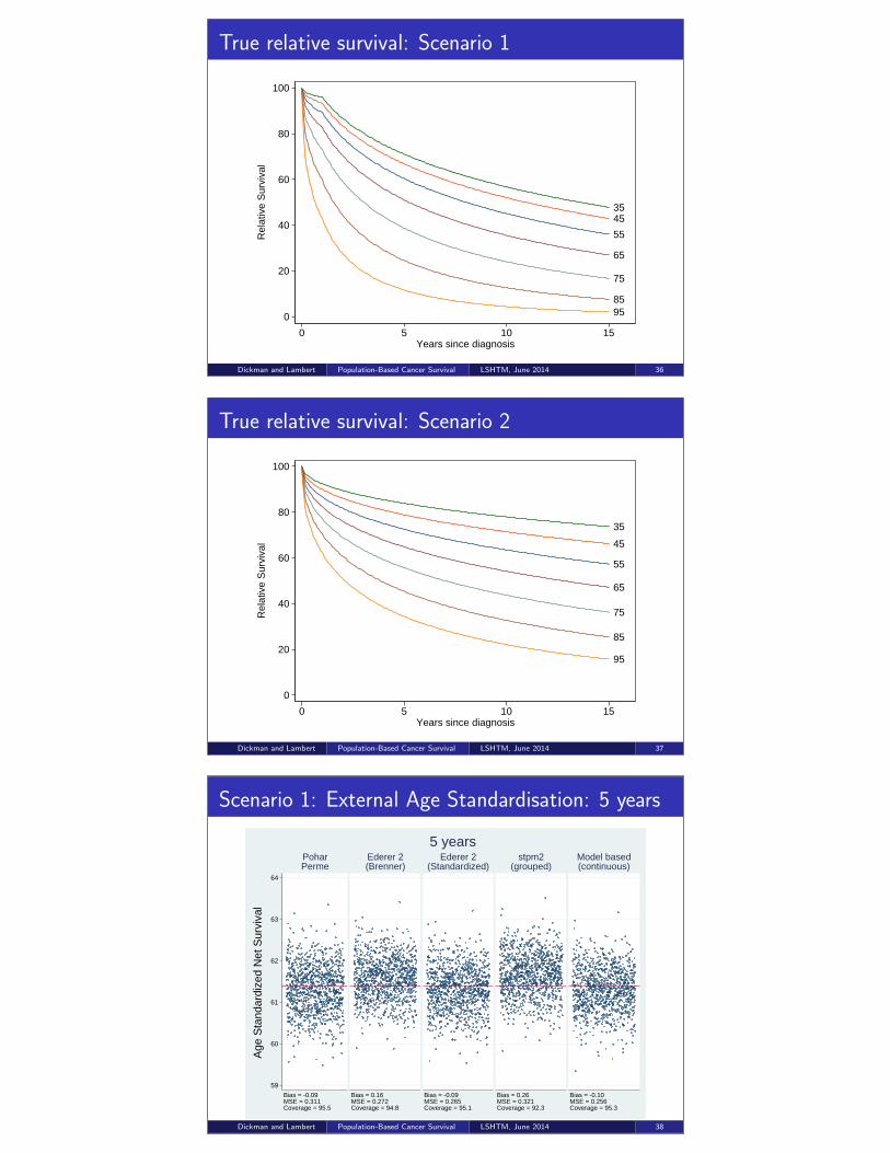
True relative survival: Scenario 1

3545

55

65

75

85950

20

40

60

80

100

Rel

ativ

e S

urvi

val

0 5 10 15Years since diagnosis


True relative survival: Scenario 2

35

45

55

65

75

85

95

0

20

40

60

80

100

Rel

ativ

e S

urvi

val

0 5 10 15Years since diagnosis


Scenario 1: External Age Standardisation: 5 years

59

60

61

62

63

64

Bias = -0.09MSE = 0.311Coverage = 95.5

PoharPerme

Bias = 0.16MSE = 0.272Coverage = 94.8

Ederer 2(Brenner)


Ederer 2(Standardized)


stpm2(grouped)


Model based(continuous)

Age

Sta

ndar

dize

d N

et S

urvi

val

5 years



48

50

52

54

56


PoharPerme


Ederer 2(Brenner)




stpm2(grouped)



Age

Sta

ndar

dize

d N

et S

urvi

val

10 years



40

45

50

55

60

65


PoharPerme


Ederer 2(Brenner)




stpm2(grouped)



Age

Sta

ndar

dize

d N

et S

urvi

val

15 years



60.00

61.00

62.00

63.00

64.00

65.00


PoharPerme


Ederer 2(Brenner)




stpm2(grouped)


Model based(continous)

Age

Sta

ndar

dize

d N

et S

urvi

val

5 years



48.00

50.00

52.00

54.00

56.00


PoharPerme


Ederer 2(Brenner)




stpm2(grouped)



Age

Sta

ndar

dize

d N

et S

urvi

val

10 years



40.00

45.00

50.00

55.00

60.00


PoharPerme


Ederer 2(Brenner)




stpm2(grouped)



Age

Sta

ndar

dize

d N

et S

urvi

val

15 years


Summary of simulation

Under these extreme scenarios, bias in Ederer II is negligiblewhen age standardising.

A theoretical bias exists, but in practice this can be ignored.

There is more variation in the Pohar Perme estimate(particularly at 10 and 15 years).

For the Ederer II method to be unbiased there needs to beeither,

1 no variation in expected survival within age groups (certainlynot true)

2 no variation in relative survival within age groups (unlikely to betrue)

However, the variation in both of these will be reduced byestimating separately within age groups.


Summary of simulation 2

The ‘cost’ of the bias when using Ederer II can effectively beignored, but there is a ‘benefit’ in using Ederer II in terms ofprecision.

The difference in the methods is small at 5 years.

Modelling (continuous age) also performs well.


The oldest age group

The methods differ most for the oldest age group (often 75+).

One can question the utility of estimating long-term net survivalof elderly patients (the hypothetical world is very different fromthe real world).

Large variation in expected survival in this age group andpossibly also large variation in net survival.

The numbers at risk as follow-up time increases will reduceproportionately more than other age groups due to highermortality due to other cases and to cancer. In the Pohar Permemethod, these individuals have a lot of weight.


Scenario 1: Age 75+

5 Years 10 Years 15 years

Pohar Perme-0.1590 -0.1613 -0.6053

2.1021 14.3727 101.831496.2 92.5 91.4

Ederer II-0.1137 -0.3198 -0.5318

1.5983 3.7299 10.042296.1 95.0 95.1

Model Based(Grouped Age)

0.8137 0.9559 0.58882.0951 3.8231 6.882790.0 92.2 94.8

Model Based(Continuous Age)

-0.5241 -0.0224 0.04511.1701 5.7305 14.770094.9 93.3 92.7

Bias, MSE and Coverage


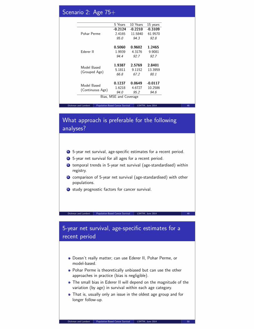
Scenario 2: Age 75+

5 Years 10 Years 15 years

Pohar Perme-0.2124 -0.2210 -0.3109

2.4165 11.5840 61.957095.0 94.3 92.8

Ederer II0.5060 0.9602 1.24651.9939 4.3176 9.908194.4 92.7 92.7

Model Based(Grouped Age)

1.9387 2.5769 2.84015.1811 9.1152 13.395966.8 67.2 80.1

Model Based(Continuous Age)

0.1237 0.0649 -0.01171.6218 4.6727 10.258694.0 95.2 94.6

Bias, MSE and Coverage


What approach is preferable for the following

analyses?

1 5-year net survival, age-specific estimates for a recent period.

2 5-year net survival for all ages for a recent period.

3 temporal trends in 5-year net survival (age-standardised) withinregistry.

4 comparison of 5-year net survival (age-standardised) with otherpopulations.

5 study prognostic factors for cancer survival.


5-year net survival, age-specific estimates for a

recent period

Doesn’t really matter; can use Ederer II, Pohar Perme, ormodel-based.

Pohar Perme is theoretically unbiased but can use the otherapproaches in practice (bias is negligible).

The small bias in Ederer II will depend on the magnitude of thevariation (by age) in survival within each age category.

That is, usually only an issue in the oldest age group and forlonger follow-up.


5-year net survival for all ages for a recent period

Unlike the previous scenario (age-specific), we must now accountfor age in the estimation procedure. That is, Ederer II applied toall patients may result in a non-negligable bias.

The Pohar Perme estimator was designed specifically for thisscenario. It accounts for age by weighting.

Can also account for age by stratification. That is, Ederer IIinternally age standardised.

Can also account for age by modelling; model-based estimation.

We prefer modelling since it has the potential to do more thanjust estimate the 5-year net survival.


Temporal trends in 5-year net survival

(age-standardised) within registry

Use either Ederer II or Pohar Perme if sufficient data, or Brenneralternative (with Ederer II) if data are sparse.

Use age distribution in last period as standard so theage-standardised estimates for that period represent the actualsurvival for patients diagnosed in that period.

Use world standard cancer population if you wish to compare topublished data that also use that standard (or if you want othersto be able to make comparisons with your data).

We like modelling!


Comparison of 5-year net survival

(age-standardised) with other populations

Use age distribution in your registry as standard if you wish tomaximise the relevance of the estimates for your specificpopulation.

Use world standard cancer population if you wish to compare topublished data that also use that standard (or if you want othersto be able to make comparisons with your data).

Be aware of differences in registration and inclusion criteria (e.g.,definition of multiple primaries). These will have a greaterimpact on the results than the choice between, for example,Ederer II and Pohar Perme.


Study prognostic factors for cancer survival

Model! But which model?

Cause-specific or excess?

Cox (only for cause-specific)

Poisson

Flexible parametric models

Other models


References

[1] Berkson J. The calculation of survival rates. In: Walters W, Gray H, Priestly J, eds.,Carcinoma and other malignant lesions of the stomach. Philadelphia: Sanders, 1942;467–484.

[2] Ederer F, Axtell L, Cutler S. The relative survival rate: A statistical methodology. NationalCancer Institute Monograph 1961;6:101–121.

[3] Ederer F, Heise H. Instructions to IBM 650 programmers in processing survivalcomputations. methodological note no. 10, end results evaluation section. Tech. rep.,National Cancer Institute, Bethesda, MD, 1959.

[4] Hakulinen T. Cancer survival corrected for heterogeneity in patient withdrawal. Biometrics1982;38:933–942.

[5] Pohar Perme M, Stare J, Esteve J. On estimation in relative survival. Biometrics 2012;68:113–120.

[6] Esteve J, Benhamou E, Croasdale M, Raymond L. Relative survival and the estimation ofnet survival: elements for further discussion. Statistics in Medicine 1990;9:529–538.

[7] Roche L, Danieli C, Belot A, Grosclaude P, Bouvier AM, Velten M, et al.. Cancer netsurvival on registry data: Use of the new unbiased Pohar-Perme estimator and magnitudeof the bias with the classical methods. Int J Cancer 2012;132:2359–69.


References 2

[8] Jooste V, Grosclaude P, Remontet L, Launoy G, Baldi I, Molinie F., et al.. Unbiasedestimates of long-term net survival of solid cancers in France. International Journal ofCancer 2013;132:2370–2377.

[9] Monnereau A, Troussard X, Belot A, Guizard AV, Woronoff AS, Bara S, et al.. Unbiasedestimates of long-term net survival of hematological malignancy patients detailed by majorsubtypes in France. International Journal of Cancer 2013;132:2378–2387.

[10] Danieli C, Remontet L, Bossard N, Roche L, Belot A. Estimating net survival: theimportance of allowing for informative censoring. Stat Med 2012;31:775–786.

[11] Dickman PW, Lambert PC, Coviello E, Rutherford MJ. Estimating net survival inpopulation-based cancer studies. Int J Cancer 2013;133:519–21.

[12] Hakulinen T. On long-term relative survival rates. J Chronic Dis 1977;30:431–443.

[13] Hakulinen T, Seppa K, Lambert PC. Choosing the relative survival method for cancersurvival estimation. European Journal of Cancer 2011;47:2202–2210.


session 18 estimating net survival { past and present · session 18 estimating net survival { past...

Documents