shallow vs deep: the great watershed in learning.amirali/public/teaching/orf523/... · shallow vs...
TRANSCRIPT

shallow vs deepthe great watershed in learning
Vikas Sindhwani
Tuesday 2nd May 2017
Topics
I ORF523 Convex and Conic Optimization
ndash Convex Optimization LPs QPs SOCPs SDPs
ndash When is an optimization problem hard Is the ldquogreat watershedrdquo(Rockafellar 1993) between convexity and nonconvexity
ndash Polynomial Optimization and Sum-of-squares Programming
I Theme Optimization Problems in Machine Learning
ndash Self-driving cars AlphaGo Detecting Cancers Machine Translationndash Is the great watershed in learning between shallow and deep
architecturesndash Nonlinear techniques at the opposite ends of Rockafellars watershed
I Kernel Methods Convex Optimization Learning polynomialsI Random embeddings scalable kernel methods shallow networksI Deep Learning Nonconvex Optimization Architectures TensorFlow
ndash Some intriguing vignettes empirical observations open questionsI How expressive are Deep NetsI Why do Deep Nets generalizeI How hard is it to train Deep Nets
2 36
Topics
I ORF523 Convex and Conic Optimization
ndash Convex Optimization LPs QPs SOCPs SDPsndash When is an optimization problem hard Is the ldquogreat watershedrdquo
(Rockafellar 1993) between convexity and nonconvexity
ndash Polynomial Optimization and Sum-of-squares Programming
I Theme Optimization Problems in Machine Learning
ndash Self-driving cars AlphaGo Detecting Cancers Machine Translationndash Is the great watershed in learning between shallow and deep
architecturesndash Nonlinear techniques at the opposite ends of Rockafellars watershed
I Kernel Methods Convex Optimization Learning polynomialsI Random embeddings scalable kernel methods shallow networksI Deep Learning Nonconvex Optimization Architectures TensorFlow
ndash Some intriguing vignettes empirical observations open questionsI How expressive are Deep NetsI Why do Deep Nets generalizeI How hard is it to train Deep Nets
2 36
Topics
I ORF523 Convex and Conic Optimization
ndash Convex Optimization LPs QPs SOCPs SDPsndash When is an optimization problem hard Is the ldquogreat watershedrdquo
(Rockafellar 1993) between convexity and nonconvexityndash Polynomial Optimization and Sum-of-squares Programming
I Theme Optimization Problems in Machine Learning
ndash Self-driving cars AlphaGo Detecting Cancers Machine Translation
ndash Is the great watershed in learning between shallow and deeparchitectures
ndash Nonlinear techniques at the opposite ends of Rockafellars watershedI Kernel Methods Convex Optimization Learning polynomialsI Random embeddings scalable kernel methods shallow networksI Deep Learning Nonconvex Optimization Architectures TensorFlow
ndash Some intriguing vignettes empirical observations open questionsI How expressive are Deep NetsI Why do Deep Nets generalizeI How hard is it to train Deep Nets
2 36
Topics
I ORF523 Convex and Conic Optimization
ndash Convex Optimization LPs QPs SOCPs SDPsndash When is an optimization problem hard Is the ldquogreat watershedrdquo
(Rockafellar 1993) between convexity and nonconvexityndash Polynomial Optimization and Sum-of-squares Programming
I Theme Optimization Problems in Machine Learning
ndash Self-driving cars AlphaGo Detecting Cancers Machine Translationndash Is the great watershed in learning between shallow and deep
architectures
ndash Nonlinear techniques at the opposite ends of Rockafellars watershedI Kernel Methods Convex Optimization Learning polynomialsI Random embeddings scalable kernel methods shallow networksI Deep Learning Nonconvex Optimization Architectures TensorFlow
ndash Some intriguing vignettes empirical observations open questionsI How expressive are Deep NetsI Why do Deep Nets generalizeI How hard is it to train Deep Nets
2 36
Topics
I ORF523 Convex and Conic Optimization
ndash Convex Optimization LPs QPs SOCPs SDPsndash When is an optimization problem hard Is the ldquogreat watershedrdquo
(Rockafellar 1993) between convexity and nonconvexityndash Polynomial Optimization and Sum-of-squares Programming
I Theme Optimization Problems in Machine Learning
ndash Self-driving cars AlphaGo Detecting Cancers Machine Translationndash Is the great watershed in learning between shallow and deep
architecturesndash Nonlinear techniques at the opposite ends of Rockafellars watershed
I Kernel Methods Convex Optimization Learning polynomialsI Random embeddings scalable kernel methods shallow networksI Deep Learning Nonconvex Optimization Architectures TensorFlow
ndash Some intriguing vignettes empirical observations open questionsI How expressive are Deep NetsI Why do Deep Nets generalizeI How hard is it to train Deep Nets
2 36
Topics
I ORF523 Convex and Conic Optimization
ndash Convex Optimization LPs QPs SOCPs SDPsndash When is an optimization problem hard Is the ldquogreat watershedrdquo
(Rockafellar 1993) between convexity and nonconvexityndash Polynomial Optimization and Sum-of-squares Programming
I Theme Optimization Problems in Machine Learning
ndash Self-driving cars AlphaGo Detecting Cancers Machine Translationndash Is the great watershed in learning between shallow and deep
architecturesndash Nonlinear techniques at the opposite ends of Rockafellars watershed
I Kernel Methods Convex Optimization Learning polynomialsI Random embeddings scalable kernel methods shallow networksI Deep Learning Nonconvex Optimization Architectures TensorFlow
ndash Some intriguing vignettes empirical observations open questionsI How expressive are Deep NetsI Why do Deep Nets generalizeI How hard is it to train Deep Nets
2 36
Setting
Estimate f X 7rarr Y from xiyili=1 sim p xi isin X yi isin Y
3 36
Setting
Estimate f X 7rarr Y from xiyili=1 sim p xi isin X yi isin Y
3 36
Regularized Loss Minimization
I Regularized Loss Minimization (GD SGD) in a suitable H
arg minfisinH
lsumi=1
V (f(xi)yi) + Ω(f)
I Understanding deep learning requires rethinking generalizationZhang et al 2017
4 36
Regularized Loss Minimization
I Regularized Loss Minimization (GD SGD) in a suitable H
arg minfisinH
lsumi=1
V (f(xi)yi) + Ω(f)
I Understanding deep learning requires rethinking generalizationZhang et al 2017
4 36
Optimization in Learning
I Optimal predictor
f = arg minf
E(xy)simpV (f(x)y)
I Approximation Error due to finite domain knowledge(Expressivity)
fH = arg minfisinH
E(xy)simpV (f(x)y)
I Estimation Error due to finite data (Generalization)
fH = arg minfisinH
lsumi=1
V (f(xi)yi) + Ω(f)
I Optimization Error finite computation (Optimization Landscape)
return f(i)H
Tractable but bad model or intractable but good model
5 36
Optimization in Learning
I Optimal predictor
f = arg minf
E(xy)simpV (f(x)y)
I Approximation Error due to finite domain knowledge(Expressivity)
fH = arg minfisinH
E(xy)simpV (f(x)y)
I Estimation Error due to finite data (Generalization)
fH = arg minfisinH
lsumi=1
V (f(xi)yi) + Ω(f)
I Optimization Error finite computation (Optimization Landscape)
return f(i)H
Tractable but bad model or intractable but good model 5 36
Nonlinearities Everywhere
Large l =rArr Big models H ldquorichrdquo non-parametricnonlinear
6 36
Nonlinearities Everywhere
Large l =rArr Big models H ldquorichrdquo non-parametricnonlinear
6 36
Nonlinearities Everywhere
Large l =rArr Big models H ldquorichrdquo non-parametricnonlinear
6 36
Choice of Nonlinear Hypothesis Space Kernels
x Ψ wTΨ(x) y
w
Ψ(x)
I eg Linear functions and Polynomials
I Infinite-dimensional nonlinear embeddings Fully non-parameteric
I Functional Analysis (Aronszajn Bergman (1950s)) Statistics (Parzen(1960s)) PDEs Numerical Analysis
I ML in 1990rsquos Nonlinear classification regression clustering time-seriesanalysis dynamical systems hypothesis testing causal modeling
I Convex Optimization
7 36
Choice of Nonlinear Hypothesis Space Deep Learning
x0 f1 f2 fL `
w1 w2 wL
z isin Rx1 x2 xLminus1 xL
I Compositions Raw data to higher abstractions (representation learning)
I Multilayer Perceptrons fl(xW) = σ(Wx) (sigmoids ReLU)I Turing (1950) In considering the functions of the mind or the brain we find certain operations which we can explain in
purely mechanical terms This we say does not correspond to the real mind it is a sort of skin which we must strip off if we are
to find the real mind Proceeding in this way do we ever come to the rdquorealrdquo mind or do we eventually come to the skin which
has nothing in it In the latter case the whole mind is mechanical
I Rosenblatt (1957) NYT 1958 New Navy Device Learns By Doing The Navy revealed the embryo of an electronic
computer today that it expects will be able to walk talk see write reproduce itself and be conscious of its existence Later
perceptrons will be able to recognize people and call out their names and instantly translate speech in one language to speech
and writing in another language it was predicted
I Perceptron (Minski and Pappert 1969) [Olarzan A Sociological Study 1996]I Backprop (1986) Reverse-mode differentiation (1960s-70s) CNNs (1980s 2012-)I Breadth-Width tradeoffsI Non-convex Optimization Domain-agnostic recipe
8 36
Choice of Nonlinear Hypothesis Space Deep Learning
x0 f1 f2 fL `
w1 w2 wL
z isin Rx1 x2 xLminus1 xL
I Compositions Raw data to higher abstractions (representation learning)I Multilayer Perceptrons fl(xW) = σ(Wx) (sigmoids ReLU)
I Turing (1950) In considering the functions of the mind or the brain we find certain operations which we can explain in
purely mechanical terms This we say does not correspond to the real mind it is a sort of skin which we must strip off if we are
to find the real mind Proceeding in this way do we ever come to the rdquorealrdquo mind or do we eventually come to the skin which
has nothing in it In the latter case the whole mind is mechanical
I Rosenblatt (1957) NYT 1958 New Navy Device Learns By Doing The Navy revealed the embryo of an electronic
computer today that it expects will be able to walk talk see write reproduce itself and be conscious of its existence Later
perceptrons will be able to recognize people and call out their names and instantly translate speech in one language to speech
and writing in another language it was predicted
I Perceptron (Minski and Pappert 1969) [Olarzan A Sociological Study 1996]I Backprop (1986) Reverse-mode differentiation (1960s-70s) CNNs (1980s 2012-)I Breadth-Width tradeoffsI Non-convex Optimization Domain-agnostic recipe
8 36
Choice of Nonlinear Hypothesis Space Deep Learning
x0 f1 f2 fL `
w1 w2 wL
z isin Rx1 x2 xLminus1 xL
I Compositions Raw data to higher abstractions (representation learning)I Multilayer Perceptrons fl(xW) = σ(Wx) (sigmoids ReLU)I Turing (1950) In considering the functions of the mind or the brain we find certain operations which we can explain in
purely mechanical terms This we say does not correspond to the real mind it is a sort of skin which we must strip off if we are
to find the real mind Proceeding in this way do we ever come to the rdquorealrdquo mind or do we eventually come to the skin which
has nothing in it In the latter case the whole mind is mechanical
I Rosenblatt (1957) NYT 1958 New Navy Device Learns By Doing The Navy revealed the embryo of an electronic
computer today that it expects will be able to walk talk see write reproduce itself and be conscious of its existence Later
perceptrons will be able to recognize people and call out their names and instantly translate speech in one language to speech
and writing in another language it was predicted
I Perceptron (Minski and Pappert 1969) [Olarzan A Sociological Study 1996]I Backprop (1986) Reverse-mode differentiation (1960s-70s) CNNs (1980s 2012-)
I Breadth-Width tradeoffsI Non-convex Optimization Domain-agnostic recipe
8 36
Choice of Nonlinear Hypothesis Space Deep Learning
x0 f1 f2 fL `
w1 w2 wL
z isin Rx1 x2 xLminus1 xL
I Compositions Raw data to higher abstractions (representation learning)I Multilayer Perceptrons fl(xW) = σ(Wx) (sigmoids ReLU)I Turing (1950) In considering the functions of the mind or the brain we find certain operations which we can explain in
purely mechanical terms This we say does not correspond to the real mind it is a sort of skin which we must strip off if we are
to find the real mind Proceeding in this way do we ever come to the rdquorealrdquo mind or do we eventually come to the skin which
has nothing in it In the latter case the whole mind is mechanical
I Rosenblatt (1957) NYT 1958 New Navy Device Learns By Doing The Navy revealed the embryo of an electronic
computer today that it expects will be able to walk talk see write reproduce itself and be conscious of its existence Later
perceptrons will be able to recognize people and call out their names and instantly translate speech in one language to speech
and writing in another language it was predicted
I Perceptron (Minski and Pappert 1969) [Olarzan A Sociological Study 1996]I Backprop (1986) Reverse-mode differentiation (1960s-70s) CNNs (1980s 2012-)I Breadth-Width tradeoffsI Non-convex Optimization Domain-agnostic recipe 8 36
The Watershed Moment Imagenet 2012
I Many statistical and computational ingredientsndash Large datasets (ILSVRC since 2010)
ndash Large statistical capacity (12M images 60M params)ndash Distributed computationndash Depth Invariant feature learning (transferrable to other tasks)ndash Engineering Dropout ReLU
I Many astonishing results since then
9 36
The Watershed Moment Imagenet 2012
I Many statistical and computational ingredientsndash Large datasets (ILSVRC since 2010)ndash Large statistical capacity (12M images 60M params)
ndash Distributed computationndash Depth Invariant feature learning (transferrable to other tasks)ndash Engineering Dropout ReLU
I Many astonishing results since then
9 36
The Watershed Moment Imagenet 2012
I Many statistical and computational ingredientsndash Large datasets (ILSVRC since 2010)ndash Large statistical capacity (12M images 60M params)ndash Distributed computation
ndash Depth Invariant feature learning (transferrable to other tasks)ndash Engineering Dropout ReLU
I Many astonishing results since then
9 36
The Watershed Moment Imagenet 2012
I Many statistical and computational ingredientsndash Large datasets (ILSVRC since 2010)ndash Large statistical capacity (12M images 60M params)ndash Distributed computationndash Depth Invariant feature learning (transferrable to other tasks)
ndash Engineering Dropout ReLU I Many astonishing results since then
9 36
The Watershed Moment Imagenet 2012
I Many statistical and computational ingredientsndash Large datasets (ILSVRC since 2010)ndash Large statistical capacity (12M images 60M params)ndash Distributed computationndash Depth Invariant feature learning (transferrable to other tasks)ndash Engineering Dropout ReLU
I Many astonishing results since then
9 36
CNNs
10 36
Self-Driving Cars
Figure End-to-End Learning for Self-driving Cars Bojarski et al 2016
11 36

Topics
I ORF523 Convex and Conic Optimization
ndash Convex Optimization LPs QPs SOCPs SDPsndash When is an optimization problem hard Is the ldquogreat watershedrdquo
(Rockafellar 1993) between convexity and nonconvexityndash Polynomial Optimization and Sum-of-squares Programming
I Theme Optimization Problems in Machine Learning
ndash Self-driving cars AlphaGo Detecting Cancers Machine Translationndash Is the great watershed in learning between shallow and deep
architecturesndash Nonlinear techniques at the opposite ends of Rockafellars watershed
I Kernel Methods Convex Optimization Learning polynomialsI Random embeddings scalable kernel methods shallow networksI Deep Learning Nonconvex Optimization Architectures TensorFlow
ndash Some intriguing vignettes empirical observations open questionsI How expressive are Deep NetsI Why do Deep Nets generalizeI How hard is it to train Deep Nets
2 36
Topics
I ORF523 Convex and Conic Optimization
ndash Convex Optimization LPs QPs SOCPs SDPsndash When is an optimization problem hard Is the ldquogreat watershedrdquo
(Rockafellar 1993) between convexity and nonconvexityndash Polynomial Optimization and Sum-of-squares Programming
I Theme Optimization Problems in Machine Learning
ndash Self-driving cars AlphaGo Detecting Cancers Machine Translation
ndash Is the great watershed in learning between shallow and deeparchitectures
ndash Nonlinear techniques at the opposite ends of Rockafellars watershedI Kernel Methods Convex Optimization Learning polynomialsI Random embeddings scalable kernel methods shallow networksI Deep Learning Nonconvex Optimization Architectures TensorFlow
ndash Some intriguing vignettes empirical observations open questionsI How expressive are Deep NetsI Why do Deep Nets generalizeI How hard is it to train Deep Nets
2 36
Topics
I ORF523 Convex and Conic Optimization
ndash Convex Optimization LPs QPs SOCPs SDPsndash When is an optimization problem hard Is the ldquogreat watershedrdquo
(Rockafellar 1993) between convexity and nonconvexityndash Polynomial Optimization and Sum-of-squares Programming
I Theme Optimization Problems in Machine Learning
ndash Self-driving cars AlphaGo Detecting Cancers Machine Translationndash Is the great watershed in learning between shallow and deep
architectures
ndash Nonlinear techniques at the opposite ends of Rockafellars watershedI Kernel Methods Convex Optimization Learning polynomialsI Random embeddings scalable kernel methods shallow networksI Deep Learning Nonconvex Optimization Architectures TensorFlow
ndash Some intriguing vignettes empirical observations open questionsI How expressive are Deep NetsI Why do Deep Nets generalizeI How hard is it to train Deep Nets
2 36
Topics
I ORF523 Convex and Conic Optimization
ndash Convex Optimization LPs QPs SOCPs SDPsndash When is an optimization problem hard Is the ldquogreat watershedrdquo
(Rockafellar 1993) between convexity and nonconvexityndash Polynomial Optimization and Sum-of-squares Programming
I Theme Optimization Problems in Machine Learning
ndash Self-driving cars AlphaGo Detecting Cancers Machine Translationndash Is the great watershed in learning between shallow and deep
architecturesndash Nonlinear techniques at the opposite ends of Rockafellars watershed
I Kernel Methods Convex Optimization Learning polynomialsI Random embeddings scalable kernel methods shallow networksI Deep Learning Nonconvex Optimization Architectures TensorFlow
ndash Some intriguing vignettes empirical observations open questionsI How expressive are Deep NetsI Why do Deep Nets generalizeI How hard is it to train Deep Nets
2 36
Topics
I ORF523 Convex and Conic Optimization
ndash Convex Optimization LPs QPs SOCPs SDPsndash When is an optimization problem hard Is the ldquogreat watershedrdquo
(Rockafellar 1993) between convexity and nonconvexityndash Polynomial Optimization and Sum-of-squares Programming
I Theme Optimization Problems in Machine Learning
ndash Self-driving cars AlphaGo Detecting Cancers Machine Translationndash Is the great watershed in learning between shallow and deep
architecturesndash Nonlinear techniques at the opposite ends of Rockafellars watershed
I Kernel Methods Convex Optimization Learning polynomialsI Random embeddings scalable kernel methods shallow networksI Deep Learning Nonconvex Optimization Architectures TensorFlow
ndash Some intriguing vignettes empirical observations open questionsI How expressive are Deep NetsI Why do Deep Nets generalizeI How hard is it to train Deep Nets
2 36
Topics
I ORF523 Convex and Conic Optimization
ndash Convex Optimization LPs QPs SOCPs SDPsndash When is an optimization problem hard Is the ldquogreat watershedrdquo
(Rockafellar 1993) between convexity and nonconvexityndash Polynomial Optimization and Sum-of-squares Programming
I Theme Optimization Problems in Machine Learning
ndash Self-driving cars AlphaGo Detecting Cancers Machine Translationndash Is the great watershed in learning between shallow and deep
architecturesndash Nonlinear techniques at the opposite ends of Rockafellars watershed
I Kernel Methods Convex Optimization Learning polynomialsI Random embeddings scalable kernel methods shallow networksI Deep Learning Nonconvex Optimization Architectures TensorFlow
ndash Some intriguing vignettes empirical observations open questionsI How expressive are Deep NetsI Why do Deep Nets generalizeI How hard is it to train Deep Nets
2 36
Setting
Estimate f X 7rarr Y from xiyili=1 sim p xi isin X yi isin Y
3 36
Setting
Estimate f X 7rarr Y from xiyili=1 sim p xi isin X yi isin Y
3 36
Regularized Loss Minimization
I Regularized Loss Minimization (GD SGD) in a suitable H
arg minfisinH
lsumi=1
V (f(xi)yi) + Ω(f)
I Understanding deep learning requires rethinking generalizationZhang et al 2017
4 36
Regularized Loss Minimization
I Regularized Loss Minimization (GD SGD) in a suitable H
arg minfisinH
lsumi=1
V (f(xi)yi) + Ω(f)
I Understanding deep learning requires rethinking generalizationZhang et al 2017
4 36
Optimization in Learning
I Optimal predictor
f = arg minf
E(xy)simpV (f(x)y)
I Approximation Error due to finite domain knowledge(Expressivity)
fH = arg minfisinH
E(xy)simpV (f(x)y)
I Estimation Error due to finite data (Generalization)
fH = arg minfisinH
lsumi=1
V (f(xi)yi) + Ω(f)
I Optimization Error finite computation (Optimization Landscape)
return f(i)H
Tractable but bad model or intractable but good model
5 36
Optimization in Learning
I Optimal predictor
f = arg minf
E(xy)simpV (f(x)y)
I Approximation Error due to finite domain knowledge(Expressivity)
fH = arg minfisinH
E(xy)simpV (f(x)y)
I Estimation Error due to finite data (Generalization)
fH = arg minfisinH
lsumi=1
V (f(xi)yi) + Ω(f)
I Optimization Error finite computation (Optimization Landscape)
return f(i)H
Tractable but bad model or intractable but good model
5 36
Optimization in Learning
I Optimal predictor
f = arg minf
E(xy)simpV (f(x)y)
I Approximation Error due to finite domain knowledge(Expressivity)
fH = arg minfisinH
E(xy)simpV (f(x)y)
I Estimation Error due to finite data (Generalization)
fH = arg minfisinH
lsumi=1
V (f(xi)yi) + Ω(f)
I Optimization Error finite computation (Optimization Landscape)
return f(i)H
Tractable but bad model or intractable but good model
5 36
Optimization in Learning
I Optimal predictor
f = arg minf
E(xy)simpV (f(x)y)
I Approximation Error due to finite domain knowledge(Expressivity)
fH = arg minfisinH
E(xy)simpV (f(x)y)
I Estimation Error due to finite data (Generalization)
fH = arg minfisinH
lsumi=1
V (f(xi)yi) + Ω(f)
I Optimization Error finite computation (Optimization Landscape)
return f(i)H
Tractable but bad model or intractable but good model
5 36
Optimization in Learning
I Optimal predictor
f = arg minf
E(xy)simpV (f(x)y)
I Approximation Error due to finite domain knowledge(Expressivity)
fH = arg minfisinH
E(xy)simpV (f(x)y)
I Estimation Error due to finite data (Generalization)
fH = arg minfisinH
lsumi=1
V (f(xi)yi) + Ω(f)
I Optimization Error finite computation (Optimization Landscape)
return f(i)H
Tractable but bad model or intractable but good model 5 36
Nonlinearities Everywhere
Large l =rArr Big models H ldquorichrdquo non-parametricnonlinear
6 36
Nonlinearities Everywhere
Large l =rArr Big models H ldquorichrdquo non-parametricnonlinear
6 36
Nonlinearities Everywhere
Large l =rArr Big models H ldquorichrdquo non-parametricnonlinear
6 36
Choice of Nonlinear Hypothesis Space Kernels
x Ψ wTΨ(x) y
w
Ψ(x)
I eg Linear functions and Polynomials
I Infinite-dimensional nonlinear embeddings Fully non-parameteric
I Functional Analysis (Aronszajn Bergman (1950s)) Statistics (Parzen(1960s)) PDEs Numerical Analysis
I ML in 1990rsquos Nonlinear classification regression clustering time-seriesanalysis dynamical systems hypothesis testing causal modeling
I Convex Optimization
7 36
Choice of Nonlinear Hypothesis Space Kernels
x Ψ wTΨ(x) y
w
Ψ(x)
I eg Linear functions and Polynomials
I Infinite-dimensional nonlinear embeddings Fully non-parameteric
I Functional Analysis (Aronszajn Bergman (1950s)) Statistics (Parzen(1960s)) PDEs Numerical Analysis
I ML in 1990rsquos Nonlinear classification regression clustering time-seriesanalysis dynamical systems hypothesis testing causal modeling
I Convex Optimization
7 36
Choice of Nonlinear Hypothesis Space Kernels
x Ψ wTΨ(x) y
w
Ψ(x)
I eg Linear functions and Polynomials
I Infinite-dimensional nonlinear embeddings Fully non-parameteric
I Functional Analysis (Aronszajn Bergman (1950s)) Statistics (Parzen(1960s)) PDEs Numerical Analysis
I ML in 1990rsquos Nonlinear classification regression clustering time-seriesanalysis dynamical systems hypothesis testing causal modeling
I Convex Optimization
7 36
Choice of Nonlinear Hypothesis Space Kernels
x Ψ wTΨ(x) y
w
Ψ(x)
I eg Linear functions and Polynomials
I Infinite-dimensional nonlinear embeddings Fully non-parameteric
I Functional Analysis (Aronszajn Bergman (1950s)) Statistics (Parzen(1960s)) PDEs Numerical Analysis
I ML in 1990rsquos Nonlinear classification regression clustering time-seriesanalysis dynamical systems hypothesis testing causal modeling
I Convex Optimization
7 36
Choice of Nonlinear Hypothesis Space Kernels
x Ψ wTΨ(x) y
w
Ψ(x)
I eg Linear functions and Polynomials
I Infinite-dimensional nonlinear embeddings Fully non-parameteric
I Functional Analysis (Aronszajn Bergman (1950s)) Statistics (Parzen(1960s)) PDEs Numerical Analysis
I ML in 1990rsquos Nonlinear classification regression clustering time-seriesanalysis dynamical systems hypothesis testing causal modeling
I Convex Optimization
7 36
Choice of Nonlinear Hypothesis Space Deep Learning
x0 f1 f2 fL `
w1 w2 wL
z isin Rx1 x2 xLminus1 xL
I Compositions Raw data to higher abstractions (representation learning)
I Multilayer Perceptrons fl(xW) = σ(Wx) (sigmoids ReLU)I Turing (1950) In considering the functions of the mind or the brain we find certain operations which we can explain in
purely mechanical terms This we say does not correspond to the real mind it is a sort of skin which we must strip off if we are
to find the real mind Proceeding in this way do we ever come to the rdquorealrdquo mind or do we eventually come to the skin which
has nothing in it In the latter case the whole mind is mechanical
I Rosenblatt (1957) NYT 1958 New Navy Device Learns By Doing The Navy revealed the embryo of an electronic
computer today that it expects will be able to walk talk see write reproduce itself and be conscious of its existence Later
perceptrons will be able to recognize people and call out their names and instantly translate speech in one language to speech
and writing in another language it was predicted
I Perceptron (Minski and Pappert 1969) [Olarzan A Sociological Study 1996]I Backprop (1986) Reverse-mode differentiation (1960s-70s) CNNs (1980s 2012-)I Breadth-Width tradeoffsI Non-convex Optimization Domain-agnostic recipe
8 36
Choice of Nonlinear Hypothesis Space Deep Learning
x0 f1 f2 fL `
w1 w2 wL
z isin Rx1 x2 xLminus1 xL
I Compositions Raw data to higher abstractions (representation learning)I Multilayer Perceptrons fl(xW) = σ(Wx) (sigmoids ReLU)
I Turing (1950) In considering the functions of the mind or the brain we find certain operations which we can explain in
purely mechanical terms This we say does not correspond to the real mind it is a sort of skin which we must strip off if we are
to find the real mind Proceeding in this way do we ever come to the rdquorealrdquo mind or do we eventually come to the skin which
has nothing in it In the latter case the whole mind is mechanical
I Rosenblatt (1957) NYT 1958 New Navy Device Learns By Doing The Navy revealed the embryo of an electronic
computer today that it expects will be able to walk talk see write reproduce itself and be conscious of its existence Later
perceptrons will be able to recognize people and call out their names and instantly translate speech in one language to speech
and writing in another language it was predicted
I Perceptron (Minski and Pappert 1969) [Olarzan A Sociological Study 1996]I Backprop (1986) Reverse-mode differentiation (1960s-70s) CNNs (1980s 2012-)I Breadth-Width tradeoffsI Non-convex Optimization Domain-agnostic recipe
8 36
Choice of Nonlinear Hypothesis Space Deep Learning
x0 f1 f2 fL `
w1 w2 wL
z isin Rx1 x2 xLminus1 xL
I Compositions Raw data to higher abstractions (representation learning)I Multilayer Perceptrons fl(xW) = σ(Wx) (sigmoids ReLU)I Turing (1950) In considering the functions of the mind or the brain we find certain operations which we can explain in
purely mechanical terms This we say does not correspond to the real mind it is a sort of skin which we must strip off if we are
to find the real mind Proceeding in this way do we ever come to the rdquorealrdquo mind or do we eventually come to the skin which
has nothing in it In the latter case the whole mind is mechanical
I Rosenblatt (1957) NYT 1958 New Navy Device Learns By Doing The Navy revealed the embryo of an electronic
computer today that it expects will be able to walk talk see write reproduce itself and be conscious of its existence Later
perceptrons will be able to recognize people and call out their names and instantly translate speech in one language to speech
and writing in another language it was predicted
I Perceptron (Minski and Pappert 1969) [Olarzan A Sociological Study 1996]I Backprop (1986) Reverse-mode differentiation (1960s-70s) CNNs (1980s 2012-)I Breadth-Width tradeoffsI Non-convex Optimization Domain-agnostic recipe
8 36
Choice of Nonlinear Hypothesis Space Deep Learning
x0 f1 f2 fL `
w1 w2 wL
z isin Rx1 x2 xLminus1 xL
I Compositions Raw data to higher abstractions (representation learning)I Multilayer Perceptrons fl(xW) = σ(Wx) (sigmoids ReLU)I Turing (1950) In considering the functions of the mind or the brain we find certain operations which we can explain in
purely mechanical terms This we say does not correspond to the real mind it is a sort of skin which we must strip off if we are
to find the real mind Proceeding in this way do we ever come to the rdquorealrdquo mind or do we eventually come to the skin which
has nothing in it In the latter case the whole mind is mechanical
I Rosenblatt (1957) NYT 1958 New Navy Device Learns By Doing The Navy revealed the embryo of an electronic
computer today that it expects will be able to walk talk see write reproduce itself and be conscious of its existence Later
perceptrons will be able to recognize people and call out their names and instantly translate speech in one language to speech
and writing in another language it was predicted
I Perceptron (Minski and Pappert 1969) [Olarzan A Sociological Study 1996]I Backprop (1986) Reverse-mode differentiation (1960s-70s) CNNs (1980s 2012-)I Breadth-Width tradeoffsI Non-convex Optimization Domain-agnostic recipe
8 36
Choice of Nonlinear Hypothesis Space Deep Learning
x0 f1 f2 fL `
w1 w2 wL
z isin Rx1 x2 xLminus1 xL
I Compositions Raw data to higher abstractions (representation learning)I Multilayer Perceptrons fl(xW) = σ(Wx) (sigmoids ReLU)I Turing (1950) In considering the functions of the mind or the brain we find certain operations which we can explain in
purely mechanical terms This we say does not correspond to the real mind it is a sort of skin which we must strip off if we are
to find the real mind Proceeding in this way do we ever come to the rdquorealrdquo mind or do we eventually come to the skin which
has nothing in it In the latter case the whole mind is mechanical
I Rosenblatt (1957) NYT 1958 New Navy Device Learns By Doing The Navy revealed the embryo of an electronic
computer today that it expects will be able to walk talk see write reproduce itself and be conscious of its existence Later
perceptrons will be able to recognize people and call out their names and instantly translate speech in one language to speech
and writing in another language it was predicted
I Perceptron (Minski and Pappert 1969) [Olarzan A Sociological Study 1996]I Backprop (1986) Reverse-mode differentiation (1960s-70s) CNNs (1980s 2012-)
I Breadth-Width tradeoffsI Non-convex Optimization Domain-agnostic recipe
8 36
Choice of Nonlinear Hypothesis Space Deep Learning
x0 f1 f2 fL `
w1 w2 wL
z isin Rx1 x2 xLminus1 xL
I Compositions Raw data to higher abstractions (representation learning)I Multilayer Perceptrons fl(xW) = σ(Wx) (sigmoids ReLU)I Turing (1950) In considering the functions of the mind or the brain we find certain operations which we can explain in
purely mechanical terms This we say does not correspond to the real mind it is a sort of skin which we must strip off if we are
to find the real mind Proceeding in this way do we ever come to the rdquorealrdquo mind or do we eventually come to the skin which
has nothing in it In the latter case the whole mind is mechanical
I Rosenblatt (1957) NYT 1958 New Navy Device Learns By Doing The Navy revealed the embryo of an electronic
computer today that it expects will be able to walk talk see write reproduce itself and be conscious of its existence Later
perceptrons will be able to recognize people and call out their names and instantly translate speech in one language to speech
and writing in another language it was predicted
I Perceptron (Minski and Pappert 1969) [Olarzan A Sociological Study 1996]I Backprop (1986) Reverse-mode differentiation (1960s-70s) CNNs (1980s 2012-)I Breadth-Width tradeoffsI Non-convex Optimization Domain-agnostic recipe 8 36
Choice of Nonlinear Hypothesis Space Deep Learning
x0 f1 f2 fL `
w1 w2 wL
z isin Rx1 x2 xLminus1 xL
I Compositions Raw data to higher abstractions (representation learning)I Multilayer Perceptrons fl(xW) = σ(Wx) (sigmoids ReLU)I Turing (1950) In considering the functions of the mind or the brain we find certain operations which we can explain in
purely mechanical terms This we say does not correspond to the real mind it is a sort of skin which we must strip off if we are
to find the real mind Proceeding in this way do we ever come to the rdquorealrdquo mind or do we eventually come to the skin which
has nothing in it In the latter case the whole mind is mechanical
I Rosenblatt (1957) NYT 1958 New Navy Device Learns By Doing The Navy revealed the embryo of an electronic
computer today that it expects will be able to walk talk see write reproduce itself and be conscious of its existence Later
perceptrons will be able to recognize people and call out their names and instantly translate speech in one language to speech
and writing in another language it was predicted
I Perceptron (Minski and Pappert 1969) [Olarzan A Sociological Study 1996]I Backprop (1986) Reverse-mode differentiation (1960s-70s) CNNs (1980s 2012-)I Breadth-Width tradeoffsI Non-convex Optimization Domain-agnostic recipe 8 36
The Watershed Moment Imagenet 2012
I Many statistical and computational ingredientsndash Large datasets (ILSVRC since 2010)
ndash Large statistical capacity (12M images 60M params)ndash Distributed computationndash Depth Invariant feature learning (transferrable to other tasks)ndash Engineering Dropout ReLU
I Many astonishing results since then
9 36
The Watershed Moment Imagenet 2012
I Many statistical and computational ingredientsndash Large datasets (ILSVRC since 2010)ndash Large statistical capacity (12M images 60M params)
ndash Distributed computationndash Depth Invariant feature learning (transferrable to other tasks)ndash Engineering Dropout ReLU
I Many astonishing results since then
9 36
The Watershed Moment Imagenet 2012
I Many statistical and computational ingredientsndash Large datasets (ILSVRC since 2010)ndash Large statistical capacity (12M images 60M params)ndash Distributed computation
ndash Depth Invariant feature learning (transferrable to other tasks)ndash Engineering Dropout ReLU
I Many astonishing results since then
9 36
The Watershed Moment Imagenet 2012
I Many statistical and computational ingredientsndash Large datasets (ILSVRC since 2010)ndash Large statistical capacity (12M images 60M params)ndash Distributed computationndash Depth Invariant feature learning (transferrable to other tasks)
ndash Engineering Dropout ReLU I Many astonishing results since then
9 36
The Watershed Moment Imagenet 2012
I Many statistical and computational ingredientsndash Large datasets (ILSVRC since 2010)ndash Large statistical capacity (12M images 60M params)ndash Distributed computationndash Depth Invariant feature learning (transferrable to other tasks)ndash Engineering Dropout ReLU
I Many astonishing results since then
9 36
CNNs
10 36
Self-Driving Cars
Figure End-to-End Learning for Self-driving Cars Bojarski et al 2016
11 36
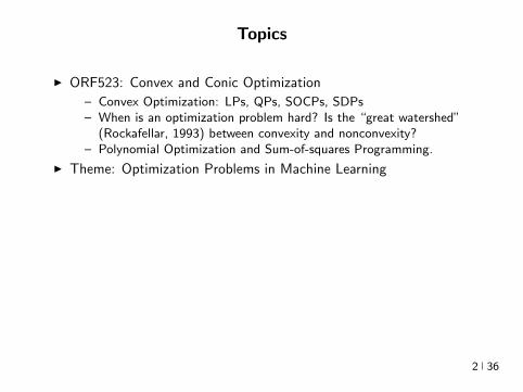
Topics
I ORF523 Convex and Conic Optimization
ndash Convex Optimization LPs QPs SOCPs SDPsndash When is an optimization problem hard Is the ldquogreat watershedrdquo
(Rockafellar 1993) between convexity and nonconvexityndash Polynomial Optimization and Sum-of-squares Programming
I Theme Optimization Problems in Machine Learning
ndash Self-driving cars AlphaGo Detecting Cancers Machine Translationndash Is the great watershed in learning between shallow and deep
architecturesndash Nonlinear techniques at the opposite ends of Rockafellars watershed
I Kernel Methods Convex Optimization Learning polynomialsI Random embeddings scalable kernel methods shallow networksI Deep Learning Nonconvex Optimization Architectures TensorFlow
ndash Some intriguing vignettes empirical observations open questionsI How expressive are Deep NetsI Why do Deep Nets generalizeI How hard is it to train Deep Nets
2 36
Topics
I ORF523 Convex and Conic Optimization
ndash Convex Optimization LPs QPs SOCPs SDPsndash When is an optimization problem hard Is the ldquogreat watershedrdquo
(Rockafellar 1993) between convexity and nonconvexityndash Polynomial Optimization and Sum-of-squares Programming
I Theme Optimization Problems in Machine Learning
ndash Self-driving cars AlphaGo Detecting Cancers Machine Translation
ndash Is the great watershed in learning between shallow and deeparchitectures
ndash Nonlinear techniques at the opposite ends of Rockafellars watershedI Kernel Methods Convex Optimization Learning polynomialsI Random embeddings scalable kernel methods shallow networksI Deep Learning Nonconvex Optimization Architectures TensorFlow
ndash Some intriguing vignettes empirical observations open questionsI How expressive are Deep NetsI Why do Deep Nets generalizeI How hard is it to train Deep Nets
2 36
Topics
I ORF523 Convex and Conic Optimization
ndash Convex Optimization LPs QPs SOCPs SDPsndash When is an optimization problem hard Is the ldquogreat watershedrdquo
(Rockafellar 1993) between convexity and nonconvexityndash Polynomial Optimization and Sum-of-squares Programming
I Theme Optimization Problems in Machine Learning
ndash Self-driving cars AlphaGo Detecting Cancers Machine Translationndash Is the great watershed in learning between shallow and deep
architectures
ndash Nonlinear techniques at the opposite ends of Rockafellars watershedI Kernel Methods Convex Optimization Learning polynomialsI Random embeddings scalable kernel methods shallow networksI Deep Learning Nonconvex Optimization Architectures TensorFlow
ndash Some intriguing vignettes empirical observations open questionsI How expressive are Deep NetsI Why do Deep Nets generalizeI How hard is it to train Deep Nets
2 36
Topics
I ORF523 Convex and Conic Optimization
ndash Convex Optimization LPs QPs SOCPs SDPsndash When is an optimization problem hard Is the ldquogreat watershedrdquo
(Rockafellar 1993) between convexity and nonconvexityndash Polynomial Optimization and Sum-of-squares Programming
I Theme Optimization Problems in Machine Learning
ndash Self-driving cars AlphaGo Detecting Cancers Machine Translationndash Is the great watershed in learning between shallow and deep
architecturesndash Nonlinear techniques at the opposite ends of Rockafellars watershed
I Kernel Methods Convex Optimization Learning polynomialsI Random embeddings scalable kernel methods shallow networksI Deep Learning Nonconvex Optimization Architectures TensorFlow
ndash Some intriguing vignettes empirical observations open questionsI How expressive are Deep NetsI Why do Deep Nets generalizeI How hard is it to train Deep Nets
2 36
Topics
I ORF523 Convex and Conic Optimization
ndash Convex Optimization LPs QPs SOCPs SDPsndash When is an optimization problem hard Is the ldquogreat watershedrdquo
(Rockafellar 1993) between convexity and nonconvexityndash Polynomial Optimization and Sum-of-squares Programming
I Theme Optimization Problems in Machine Learning
ndash Self-driving cars AlphaGo Detecting Cancers Machine Translationndash Is the great watershed in learning between shallow and deep
architecturesndash Nonlinear techniques at the opposite ends of Rockafellars watershed
I Kernel Methods Convex Optimization Learning polynomialsI Random embeddings scalable kernel methods shallow networksI Deep Learning Nonconvex Optimization Architectures TensorFlow
ndash Some intriguing vignettes empirical observations open questionsI How expressive are Deep NetsI Why do Deep Nets generalizeI How hard is it to train Deep Nets
2 36
Topics
I ORF523 Convex and Conic Optimization
ndash Convex Optimization LPs QPs SOCPs SDPsndash When is an optimization problem hard Is the ldquogreat watershedrdquo
(Rockafellar 1993) between convexity and nonconvexityndash Polynomial Optimization and Sum-of-squares Programming
I Theme Optimization Problems in Machine Learning
ndash Self-driving cars AlphaGo Detecting Cancers Machine Translationndash Is the great watershed in learning between shallow and deep
architecturesndash Nonlinear techniques at the opposite ends of Rockafellars watershed
I Kernel Methods Convex Optimization Learning polynomialsI Random embeddings scalable kernel methods shallow networksI Deep Learning Nonconvex Optimization Architectures TensorFlow
ndash Some intriguing vignettes empirical observations open questionsI How expressive are Deep NetsI Why do Deep Nets generalizeI How hard is it to train Deep Nets
2 36
Setting
Estimate f X 7rarr Y from xiyili=1 sim p xi isin X yi isin Y
3 36
Setting
Estimate f X 7rarr Y from xiyili=1 sim p xi isin X yi isin Y
3 36
Regularized Loss Minimization
I Regularized Loss Minimization (GD SGD) in a suitable H
arg minfisinH
lsumi=1
V (f(xi)yi) + Ω(f)
I Understanding deep learning requires rethinking generalizationZhang et al 2017
4 36
Regularized Loss Minimization
I Regularized Loss Minimization (GD SGD) in a suitable H
arg minfisinH
lsumi=1
V (f(xi)yi) + Ω(f)
I Understanding deep learning requires rethinking generalizationZhang et al 2017
4 36
Optimization in Learning
I Optimal predictor
f = arg minf
E(xy)simpV (f(x)y)
I Approximation Error due to finite domain knowledge(Expressivity)
fH = arg minfisinH
E(xy)simpV (f(x)y)
I Estimation Error due to finite data (Generalization)
fH = arg minfisinH
lsumi=1
V (f(xi)yi) + Ω(f)
I Optimization Error finite computation (Optimization Landscape)
return f(i)H
Tractable but bad model or intractable but good model
5 36
Optimization in Learning
I Optimal predictor
f = arg minf
E(xy)simpV (f(x)y)
I Approximation Error due to finite domain knowledge(Expressivity)
fH = arg minfisinH
E(xy)simpV (f(x)y)
I Estimation Error due to finite data (Generalization)
fH = arg minfisinH
lsumi=1
V (f(xi)yi) + Ω(f)
I Optimization Error finite computation (Optimization Landscape)
return f(i)H
Tractable but bad model or intractable but good model
5 36
Optimization in Learning
I Optimal predictor
f = arg minf
E(xy)simpV (f(x)y)
I Approximation Error due to finite domain knowledge(Expressivity)
fH = arg minfisinH
E(xy)simpV (f(x)y)
I Estimation Error due to finite data (Generalization)
fH = arg minfisinH
lsumi=1
V (f(xi)yi) + Ω(f)
I Optimization Error finite computation (Optimization Landscape)
return f(i)H
Tractable but bad model or intractable but good model
5 36
Optimization in Learning
I Optimal predictor
f = arg minf
E(xy)simpV (f(x)y)
I Approximation Error due to finite domain knowledge(Expressivity)
fH = arg minfisinH
E(xy)simpV (f(x)y)
I Estimation Error due to finite data (Generalization)
fH = arg minfisinH
lsumi=1
V (f(xi)yi) + Ω(f)
I Optimization Error finite computation (Optimization Landscape)
return f(i)H
Tractable but bad model or intractable but good model
5 36
Optimization in Learning
I Optimal predictor
f = arg minf
E(xy)simpV (f(x)y)
I Approximation Error due to finite domain knowledge(Expressivity)
fH = arg minfisinH
E(xy)simpV (f(x)y)
I Estimation Error due to finite data (Generalization)
fH = arg minfisinH
lsumi=1
V (f(xi)yi) + Ω(f)
I Optimization Error finite computation (Optimization Landscape)
return f(i)H
Tractable but bad model or intractable but good model 5 36
Nonlinearities Everywhere
Large l =rArr Big models H ldquorichrdquo non-parametricnonlinear
6 36
Nonlinearities Everywhere
Large l =rArr Big models H ldquorichrdquo non-parametricnonlinear
6 36
Nonlinearities Everywhere
Large l =rArr Big models H ldquorichrdquo non-parametricnonlinear
6 36
Choice of Nonlinear Hypothesis Space Kernels
x Ψ wTΨ(x) y
w
Ψ(x)
I eg Linear functions and Polynomials
I Infinite-dimensional nonlinear embeddings Fully non-parameteric
I Functional Analysis (Aronszajn Bergman (1950s)) Statistics (Parzen(1960s)) PDEs Numerical Analysis
I ML in 1990rsquos Nonlinear classification regression clustering time-seriesanalysis dynamical systems hypothesis testing causal modeling
I Convex Optimization
7 36
Choice of Nonlinear Hypothesis Space Kernels
x Ψ wTΨ(x) y
w
Ψ(x)
I eg Linear functions and Polynomials
I Infinite-dimensional nonlinear embeddings Fully non-parameteric
I Functional Analysis (Aronszajn Bergman (1950s)) Statistics (Parzen(1960s)) PDEs Numerical Analysis
I ML in 1990rsquos Nonlinear classification regression clustering time-seriesanalysis dynamical systems hypothesis testing causal modeling
I Convex Optimization
7 36
Choice of Nonlinear Hypothesis Space Kernels
x Ψ wTΨ(x) y
w
Ψ(x)
I eg Linear functions and Polynomials
I Infinite-dimensional nonlinear embeddings Fully non-parameteric
I Functional Analysis (Aronszajn Bergman (1950s)) Statistics (Parzen(1960s)) PDEs Numerical Analysis
I ML in 1990rsquos Nonlinear classification regression clustering time-seriesanalysis dynamical systems hypothesis testing causal modeling
I Convex Optimization
7 36
Choice of Nonlinear Hypothesis Space Kernels
x Ψ wTΨ(x) y
w
Ψ(x)
I eg Linear functions and Polynomials
I Infinite-dimensional nonlinear embeddings Fully non-parameteric
I Functional Analysis (Aronszajn Bergman (1950s)) Statistics (Parzen(1960s)) PDEs Numerical Analysis
I ML in 1990rsquos Nonlinear classification regression clustering time-seriesanalysis dynamical systems hypothesis testing causal modeling
I Convex Optimization
7 36
Choice of Nonlinear Hypothesis Space Kernels
x Ψ wTΨ(x) y
w
Ψ(x)
I eg Linear functions and Polynomials
I Infinite-dimensional nonlinear embeddings Fully non-parameteric
I Functional Analysis (Aronszajn Bergman (1950s)) Statistics (Parzen(1960s)) PDEs Numerical Analysis
I ML in 1990rsquos Nonlinear classification regression clustering time-seriesanalysis dynamical systems hypothesis testing causal modeling
I Convex Optimization
7 36
Choice of Nonlinear Hypothesis Space Deep Learning
x0 f1 f2 fL `
w1 w2 wL
z isin Rx1 x2 xLminus1 xL
I Compositions Raw data to higher abstractions (representation learning)
I Multilayer Perceptrons fl(xW) = σ(Wx) (sigmoids ReLU)I Turing (1950) In considering the functions of the mind or the brain we find certain operations which we can explain in
purely mechanical terms This we say does not correspond to the real mind it is a sort of skin which we must strip off if we are
to find the real mind Proceeding in this way do we ever come to the rdquorealrdquo mind or do we eventually come to the skin which
has nothing in it In the latter case the whole mind is mechanical
I Rosenblatt (1957) NYT 1958 New Navy Device Learns By Doing The Navy revealed the embryo of an electronic
computer today that it expects will be able to walk talk see write reproduce itself and be conscious of its existence Later
perceptrons will be able to recognize people and call out their names and instantly translate speech in one language to speech
and writing in another language it was predicted
I Perceptron (Minski and Pappert 1969) [Olarzan A Sociological Study 1996]I Backprop (1986) Reverse-mode differentiation (1960s-70s) CNNs (1980s 2012-)I Breadth-Width tradeoffsI Non-convex Optimization Domain-agnostic recipe
8 36
Choice of Nonlinear Hypothesis Space Deep Learning
x0 f1 f2 fL `
w1 w2 wL
z isin Rx1 x2 xLminus1 xL
I Compositions Raw data to higher abstractions (representation learning)I Multilayer Perceptrons fl(xW) = σ(Wx) (sigmoids ReLU)
I Turing (1950) In considering the functions of the mind or the brain we find certain operations which we can explain in
purely mechanical terms This we say does not correspond to the real mind it is a sort of skin which we must strip off if we are
to find the real mind Proceeding in this way do we ever come to the rdquorealrdquo mind or do we eventually come to the skin which
has nothing in it In the latter case the whole mind is mechanical
I Rosenblatt (1957) NYT 1958 New Navy Device Learns By Doing The Navy revealed the embryo of an electronic
computer today that it expects will be able to walk talk see write reproduce itself and be conscious of its existence Later
perceptrons will be able to recognize people and call out their names and instantly translate speech in one language to speech
and writing in another language it was predicted
I Perceptron (Minski and Pappert 1969) [Olarzan A Sociological Study 1996]I Backprop (1986) Reverse-mode differentiation (1960s-70s) CNNs (1980s 2012-)I Breadth-Width tradeoffsI Non-convex Optimization Domain-agnostic recipe
8 36
Choice of Nonlinear Hypothesis Space Deep Learning
x0 f1 f2 fL `
w1 w2 wL
z isin Rx1 x2 xLminus1 xL
I Compositions Raw data to higher abstractions (representation learning)I Multilayer Perceptrons fl(xW) = σ(Wx) (sigmoids ReLU)I Turing (1950) In considering the functions of the mind or the brain we find certain operations which we can explain in
purely mechanical terms This we say does not correspond to the real mind it is a sort of skin which we must strip off if we are
to find the real mind Proceeding in this way do we ever come to the rdquorealrdquo mind or do we eventually come to the skin which
has nothing in it In the latter case the whole mind is mechanical
I Rosenblatt (1957) NYT 1958 New Navy Device Learns By Doing The Navy revealed the embryo of an electronic
computer today that it expects will be able to walk talk see write reproduce itself and be conscious of its existence Later
perceptrons will be able to recognize people and call out their names and instantly translate speech in one language to speech
and writing in another language it was predicted
I Perceptron (Minski and Pappert 1969) [Olarzan A Sociological Study 1996]I Backprop (1986) Reverse-mode differentiation (1960s-70s) CNNs (1980s 2012-)I Breadth-Width tradeoffsI Non-convex Optimization Domain-agnostic recipe
8 36
Choice of Nonlinear Hypothesis Space Deep Learning
x0 f1 f2 fL `
w1 w2 wL
z isin Rx1 x2 xLminus1 xL
I Compositions Raw data to higher abstractions (representation learning)I Multilayer Perceptrons fl(xW) = σ(Wx) (sigmoids ReLU)I Turing (1950) In considering the functions of the mind or the brain we find certain operations which we can explain in
purely mechanical terms This we say does not correspond to the real mind it is a sort of skin which we must strip off if we are
to find the real mind Proceeding in this way do we ever come to the rdquorealrdquo mind or do we eventually come to the skin which
has nothing in it In the latter case the whole mind is mechanical
I Rosenblatt (1957) NYT 1958 New Navy Device Learns By Doing The Navy revealed the embryo of an electronic
computer today that it expects will be able to walk talk see write reproduce itself and be conscious of its existence Later
perceptrons will be able to recognize people and call out their names and instantly translate speech in one language to speech
and writing in another language it was predicted
I Perceptron (Minski and Pappert 1969) [Olarzan A Sociological Study 1996]I Backprop (1986) Reverse-mode differentiation (1960s-70s) CNNs (1980s 2012-)I Breadth-Width tradeoffsI Non-convex Optimization Domain-agnostic recipe
8 36
Choice of Nonlinear Hypothesis Space Deep Learning
x0 f1 f2 fL `
w1 w2 wL
z isin Rx1 x2 xLminus1 xL
I Compositions Raw data to higher abstractions (representation learning)I Multilayer Perceptrons fl(xW) = σ(Wx) (sigmoids ReLU)I Turing (1950) In considering the functions of the mind or the brain we find certain operations which we can explain in
purely mechanical terms This we say does not correspond to the real mind it is a sort of skin which we must strip off if we are
to find the real mind Proceeding in this way do we ever come to the rdquorealrdquo mind or do we eventually come to the skin which
has nothing in it In the latter case the whole mind is mechanical
I Rosenblatt (1957) NYT 1958 New Navy Device Learns By Doing The Navy revealed the embryo of an electronic
computer today that it expects will be able to walk talk see write reproduce itself and be conscious of its existence Later
perceptrons will be able to recognize people and call out their names and instantly translate speech in one language to speech
and writing in another language it was predicted
I Perceptron (Minski and Pappert 1969) [Olarzan A Sociological Study 1996]I Backprop (1986) Reverse-mode differentiation (1960s-70s) CNNs (1980s 2012-)
I Breadth-Width tradeoffsI Non-convex Optimization Domain-agnostic recipe
8 36
Choice of Nonlinear Hypothesis Space Deep Learning
x0 f1 f2 fL `
w1 w2 wL
z isin Rx1 x2 xLminus1 xL
I Compositions Raw data to higher abstractions (representation learning)I Multilayer Perceptrons fl(xW) = σ(Wx) (sigmoids ReLU)I Turing (1950) In considering the functions of the mind or the brain we find certain operations which we can explain in
purely mechanical terms This we say does not correspond to the real mind it is a sort of skin which we must strip off if we are
to find the real mind Proceeding in this way do we ever come to the rdquorealrdquo mind or do we eventually come to the skin which
has nothing in it In the latter case the whole mind is mechanical
I Rosenblatt (1957) NYT 1958 New Navy Device Learns By Doing The Navy revealed the embryo of an electronic
computer today that it expects will be able to walk talk see write reproduce itself and be conscious of its existence Later
perceptrons will be able to recognize people and call out their names and instantly translate speech in one language to speech
and writing in another language it was predicted
I Perceptron (Minski and Pappert 1969) [Olarzan A Sociological Study 1996]I Backprop (1986) Reverse-mode differentiation (1960s-70s) CNNs (1980s 2012-)I Breadth-Width tradeoffsI Non-convex Optimization Domain-agnostic recipe 8 36
Choice of Nonlinear Hypothesis Space Deep Learning
x0 f1 f2 fL `
w1 w2 wL
z isin Rx1 x2 xLminus1 xL
I Compositions Raw data to higher abstractions (representation learning)I Multilayer Perceptrons fl(xW) = σ(Wx) (sigmoids ReLU)I Turing (1950) In considering the functions of the mind or the brain we find certain operations which we can explain in
purely mechanical terms This we say does not correspond to the real mind it is a sort of skin which we must strip off if we are
to find the real mind Proceeding in this way do we ever come to the rdquorealrdquo mind or do we eventually come to the skin which
has nothing in it In the latter case the whole mind is mechanical
I Rosenblatt (1957) NYT 1958 New Navy Device Learns By Doing The Navy revealed the embryo of an electronic
computer today that it expects will be able to walk talk see write reproduce itself and be conscious of its existence Later
perceptrons will be able to recognize people and call out their names and instantly translate speech in one language to speech
and writing in another language it was predicted
I Perceptron (Minski and Pappert 1969) [Olarzan A Sociological Study 1996]I Backprop (1986) Reverse-mode differentiation (1960s-70s) CNNs (1980s 2012-)I Breadth-Width tradeoffsI Non-convex Optimization Domain-agnostic recipe 8 36
The Watershed Moment Imagenet 2012
I Many statistical and computational ingredientsndash Large datasets (ILSVRC since 2010)
ndash Large statistical capacity (12M images 60M params)ndash Distributed computationndash Depth Invariant feature learning (transferrable to other tasks)ndash Engineering Dropout ReLU
I Many astonishing results since then
9 36
The Watershed Moment Imagenet 2012
I Many statistical and computational ingredientsndash Large datasets (ILSVRC since 2010)ndash Large statistical capacity (12M images 60M params)
ndash Distributed computationndash Depth Invariant feature learning (transferrable to other tasks)ndash Engineering Dropout ReLU
I Many astonishing results since then
9 36
The Watershed Moment Imagenet 2012
I Many statistical and computational ingredientsndash Large datasets (ILSVRC since 2010)ndash Large statistical capacity (12M images 60M params)ndash Distributed computation
ndash Depth Invariant feature learning (transferrable to other tasks)ndash Engineering Dropout ReLU
I Many astonishing results since then
9 36
The Watershed Moment Imagenet 2012
I Many statistical and computational ingredientsndash Large datasets (ILSVRC since 2010)ndash Large statistical capacity (12M images 60M params)ndash Distributed computationndash Depth Invariant feature learning (transferrable to other tasks)
ndash Engineering Dropout ReLU I Many astonishing results since then
9 36
The Watershed Moment Imagenet 2012
I Many statistical and computational ingredientsndash Large datasets (ILSVRC since 2010)ndash Large statistical capacity (12M images 60M params)ndash Distributed computationndash Depth Invariant feature learning (transferrable to other tasks)ndash Engineering Dropout ReLU
I Many astonishing results since then
9 36
CNNs
10 36
Self-Driving Cars
Figure End-to-End Learning for Self-driving Cars Bojarski et al 2016
11 36

Topics
I ORF523 Convex and Conic Optimization
ndash Convex Optimization LPs QPs SOCPs SDPsndash When is an optimization problem hard Is the ldquogreat watershedrdquo
(Rockafellar 1993) between convexity and nonconvexityndash Polynomial Optimization and Sum-of-squares Programming
I Theme Optimization Problems in Machine Learning
ndash Self-driving cars AlphaGo Detecting Cancers Machine Translationndash Is the great watershed in learning between shallow and deep
architectures
ndash Nonlinear techniques at the opposite ends of Rockafellars watershedI Kernel Methods Convex Optimization Learning polynomialsI Random embeddings scalable kernel methods shallow networksI Deep Learning Nonconvex Optimization Architectures TensorFlow
ndash Some intriguing vignettes empirical observations open questionsI How expressive are Deep NetsI Why do Deep Nets generalizeI How hard is it to train Deep Nets
2 36
Topics
I ORF523 Convex and Conic Optimization
ndash Convex Optimization LPs QPs SOCPs SDPsndash When is an optimization problem hard Is the ldquogreat watershedrdquo
(Rockafellar 1993) between convexity and nonconvexityndash Polynomial Optimization and Sum-of-squares Programming
I Theme Optimization Problems in Machine Learning
ndash Self-driving cars AlphaGo Detecting Cancers Machine Translationndash Is the great watershed in learning between shallow and deep
architecturesndash Nonlinear techniques at the opposite ends of Rockafellars watershed
I Kernel Methods Convex Optimization Learning polynomialsI Random embeddings scalable kernel methods shallow networksI Deep Learning Nonconvex Optimization Architectures TensorFlow
ndash Some intriguing vignettes empirical observations open questionsI How expressive are Deep NetsI Why do Deep Nets generalizeI How hard is it to train Deep Nets
2 36
Topics
I ORF523 Convex and Conic Optimization
ndash Convex Optimization LPs QPs SOCPs SDPsndash When is an optimization problem hard Is the ldquogreat watershedrdquo
(Rockafellar 1993) between convexity and nonconvexityndash Polynomial Optimization and Sum-of-squares Programming
I Theme Optimization Problems in Machine Learning
ndash Self-driving cars AlphaGo Detecting Cancers Machine Translationndash Is the great watershed in learning between shallow and deep
architecturesndash Nonlinear techniques at the opposite ends of Rockafellars watershed
I Kernel Methods Convex Optimization Learning polynomialsI Random embeddings scalable kernel methods shallow networksI Deep Learning Nonconvex Optimization Architectures TensorFlow
ndash Some intriguing vignettes empirical observations open questionsI How expressive are Deep NetsI Why do Deep Nets generalizeI How hard is it to train Deep Nets
2 36
Topics
I ORF523 Convex and Conic Optimization
ndash Convex Optimization LPs QPs SOCPs SDPsndash When is an optimization problem hard Is the ldquogreat watershedrdquo
(Rockafellar 1993) between convexity and nonconvexityndash Polynomial Optimization and Sum-of-squares Programming
I Theme Optimization Problems in Machine Learning
ndash Self-driving cars AlphaGo Detecting Cancers Machine Translationndash Is the great watershed in learning between shallow and deep
architecturesndash Nonlinear techniques at the opposite ends of Rockafellars watershed
I Kernel Methods Convex Optimization Learning polynomialsI Random embeddings scalable kernel methods shallow networksI Deep Learning Nonconvex Optimization Architectures TensorFlow
ndash Some intriguing vignettes empirical observations open questionsI How expressive are Deep NetsI Why do Deep Nets generalizeI How hard is it to train Deep Nets
2 36
Setting
Estimate f X 7rarr Y from xiyili=1 sim p xi isin X yi isin Y
3 36
Setting
Estimate f X 7rarr Y from xiyili=1 sim p xi isin X yi isin Y
3 36
Regularized Loss Minimization
I Regularized Loss Minimization (GD SGD) in a suitable H
arg minfisinH
lsumi=1
V (f(xi)yi) + Ω(f)
I Understanding deep learning requires rethinking generalizationZhang et al 2017
4 36
Regularized Loss Minimization
I Regularized Loss Minimization (GD SGD) in a suitable H
arg minfisinH
lsumi=1
V (f(xi)yi) + Ω(f)
I Understanding deep learning requires rethinking generalizationZhang et al 2017
4 36
Optimization in Learning
I Optimal predictor
f = arg minf
E(xy)simpV (f(x)y)
I Approximation Error due to finite domain knowledge(Expressivity)
fH = arg minfisinH
E(xy)simpV (f(x)y)
I Estimation Error due to finite data (Generalization)
fH = arg minfisinH
lsumi=1
V (f(xi)yi) + Ω(f)
I Optimization Error finite computation (Optimization Landscape)
return f(i)H
Tractable but bad model or intractable but good model
5 36
Optimization in Learning
I Optimal predictor
f = arg minf
E(xy)simpV (f(x)y)
I Approximation Error due to finite domain knowledge(Expressivity)
fH = arg minfisinH
E(xy)simpV (f(x)y)
I Estimation Error due to finite data (Generalization)
fH = arg minfisinH
lsumi=1
V (f(xi)yi) + Ω(f)
I Optimization Error finite computation (Optimization Landscape)
return f(i)H
Tractable but bad model or intractable but good model
5 36
Optimization in Learning
I Optimal predictor
f = arg minf
E(xy)simpV (f(x)y)
I Approximation Error due to finite domain knowledge(Expressivity)
fH = arg minfisinH
E(xy)simpV (f(x)y)
I Estimation Error due to finite data (Generalization)
fH = arg minfisinH
lsumi=1
V (f(xi)yi) + Ω(f)
I Optimization Error finite computation (Optimization Landscape)
return f(i)H
Tractable but bad model or intractable but good model
5 36
Optimization in Learning
I Optimal predictor
f = arg minf
E(xy)simpV (f(x)y)
I Approximation Error due to finite domain knowledge(Expressivity)
fH = arg minfisinH
E(xy)simpV (f(x)y)
I Estimation Error due to finite data (Generalization)
fH = arg minfisinH
lsumi=1
V (f(xi)yi) + Ω(f)
I Optimization Error finite computation (Optimization Landscape)
return f(i)H
Tractable but bad model or intractable but good model
5 36
Optimization in Learning
I Optimal predictor
f = arg minf
E(xy)simpV (f(x)y)
I Approximation Error due to finite domain knowledge(Expressivity)
fH = arg minfisinH
E(xy)simpV (f(x)y)
I Estimation Error due to finite data (Generalization)
fH = arg minfisinH
lsumi=1
V (f(xi)yi) + Ω(f)
I Optimization Error finite computation (Optimization Landscape)
return f(i)H
Tractable but bad model or intractable but good model 5 36
Nonlinearities Everywhere
Large l =rArr Big models H ldquorichrdquo non-parametricnonlinear
6 36
Nonlinearities Everywhere
Large l =rArr Big models H ldquorichrdquo non-parametricnonlinear
6 36
Nonlinearities Everywhere
Large l =rArr Big models H ldquorichrdquo non-parametricnonlinear
6 36
Choice of Nonlinear Hypothesis Space Kernels
x Ψ wTΨ(x) y
w
Ψ(x)
I eg Linear functions and Polynomials
I Infinite-dimensional nonlinear embeddings Fully non-parameteric
I Functional Analysis (Aronszajn Bergman (1950s)) Statistics (Parzen(1960s)) PDEs Numerical Analysis
I ML in 1990rsquos Nonlinear classification regression clustering time-seriesanalysis dynamical systems hypothesis testing causal modeling
I Convex Optimization
7 36
Choice of Nonlinear Hypothesis Space Kernels
x Ψ wTΨ(x) y
w
Ψ(x)
I eg Linear functions and Polynomials
I Infinite-dimensional nonlinear embeddings Fully non-parameteric
I Functional Analysis (Aronszajn Bergman (1950s)) Statistics (Parzen(1960s)) PDEs Numerical Analysis
I ML in 1990rsquos Nonlinear classification regression clustering time-seriesanalysis dynamical systems hypothesis testing causal modeling
I Convex Optimization
7 36
Choice of Nonlinear Hypothesis Space Kernels
x Ψ wTΨ(x) y
w
Ψ(x)
I eg Linear functions and Polynomials
I Infinite-dimensional nonlinear embeddings Fully non-parameteric
I Functional Analysis (Aronszajn Bergman (1950s)) Statistics (Parzen(1960s)) PDEs Numerical Analysis
I ML in 1990rsquos Nonlinear classification regression clustering time-seriesanalysis dynamical systems hypothesis testing causal modeling
I Convex Optimization
7 36
Choice of Nonlinear Hypothesis Space Kernels
x Ψ wTΨ(x) y
w
Ψ(x)
I eg Linear functions and Polynomials
I Infinite-dimensional nonlinear embeddings Fully non-parameteric
I Functional Analysis (Aronszajn Bergman (1950s)) Statistics (Parzen(1960s)) PDEs Numerical Analysis
I ML in 1990rsquos Nonlinear classification regression clustering time-seriesanalysis dynamical systems hypothesis testing causal modeling
I Convex Optimization
7 36
Choice of Nonlinear Hypothesis Space Kernels
x Ψ wTΨ(x) y
w
Ψ(x)
I eg Linear functions and Polynomials
I Infinite-dimensional nonlinear embeddings Fully non-parameteric
I Functional Analysis (Aronszajn Bergman (1950s)) Statistics (Parzen(1960s)) PDEs Numerical Analysis
I ML in 1990rsquos Nonlinear classification regression clustering time-seriesanalysis dynamical systems hypothesis testing causal modeling
I Convex Optimization
7 36
Choice of Nonlinear Hypothesis Space Deep Learning
x0 f1 f2 fL `
w1 w2 wL
z isin Rx1 x2 xLminus1 xL
I Compositions Raw data to higher abstractions (representation learning)
I Multilayer Perceptrons fl(xW) = σ(Wx) (sigmoids ReLU)I Turing (1950) In considering the functions of the mind or the brain we find certain operations which we can explain in
purely mechanical terms This we say does not correspond to the real mind it is a sort of skin which we must strip off if we are
to find the real mind Proceeding in this way do we ever come to the rdquorealrdquo mind or do we eventually come to the skin which
has nothing in it In the latter case the whole mind is mechanical
I Rosenblatt (1957) NYT 1958 New Navy Device Learns By Doing The Navy revealed the embryo of an electronic
computer today that it expects will be able to walk talk see write reproduce itself and be conscious of its existence Later
perceptrons will be able to recognize people and call out their names and instantly translate speech in one language to speech
and writing in another language it was predicted
I Perceptron (Minski and Pappert 1969) [Olarzan A Sociological Study 1996]I Backprop (1986) Reverse-mode differentiation (1960s-70s) CNNs (1980s 2012-)I Breadth-Width tradeoffsI Non-convex Optimization Domain-agnostic recipe
8 36
Choice of Nonlinear Hypothesis Space Deep Learning
x0 f1 f2 fL `
w1 w2 wL
z isin Rx1 x2 xLminus1 xL
I Compositions Raw data to higher abstractions (representation learning)I Multilayer Perceptrons fl(xW) = σ(Wx) (sigmoids ReLU)
I Turing (1950) In considering the functions of the mind or the brain we find certain operations which we can explain in
purely mechanical terms This we say does not correspond to the real mind it is a sort of skin which we must strip off if we are
to find the real mind Proceeding in this way do we ever come to the rdquorealrdquo mind or do we eventually come to the skin which
has nothing in it In the latter case the whole mind is mechanical
I Rosenblatt (1957) NYT 1958 New Navy Device Learns By Doing The Navy revealed the embryo of an electronic
computer today that it expects will be able to walk talk see write reproduce itself and be conscious of its existence Later
perceptrons will be able to recognize people and call out their names and instantly translate speech in one language to speech
and writing in another language it was predicted
I Perceptron (Minski and Pappert 1969) [Olarzan A Sociological Study 1996]I Backprop (1986) Reverse-mode differentiation (1960s-70s) CNNs (1980s 2012-)I Breadth-Width tradeoffsI Non-convex Optimization Domain-agnostic recipe
8 36
Choice of Nonlinear Hypothesis Space Deep Learning
x0 f1 f2 fL `
w1 w2 wL
z isin Rx1 x2 xLminus1 xL
I Compositions Raw data to higher abstractions (representation learning)I Multilayer Perceptrons fl(xW) = σ(Wx) (sigmoids ReLU)I Turing (1950) In considering the functions of the mind or the brain we find certain operations which we can explain in
purely mechanical terms This we say does not correspond to the real mind it is a sort of skin which we must strip off if we are
to find the real mind Proceeding in this way do we ever come to the rdquorealrdquo mind or do we eventually come to the skin which
has nothing in it In the latter case the whole mind is mechanical
I Rosenblatt (1957) NYT 1958 New Navy Device Learns By Doing The Navy revealed the embryo of an electronic
computer today that it expects will be able to walk talk see write reproduce itself and be conscious of its existence Later
perceptrons will be able to recognize people and call out their names and instantly translate speech in one language to speech
and writing in another language it was predicted
I Perceptron (Minski and Pappert 1969) [Olarzan A Sociological Study 1996]I Backprop (1986) Reverse-mode differentiation (1960s-70s) CNNs (1980s 2012-)I Breadth-Width tradeoffsI Non-convex Optimization Domain-agnostic recipe
8 36
Choice of Nonlinear Hypothesis Space Deep Learning
x0 f1 f2 fL `
w1 w2 wL
z isin Rx1 x2 xLminus1 xL
I Compositions Raw data to higher abstractions (representation learning)I Multilayer Perceptrons fl(xW) = σ(Wx) (sigmoids ReLU)I Turing (1950) In considering the functions of the mind or the brain we find certain operations which we can explain in
purely mechanical terms This we say does not correspond to the real mind it is a sort of skin which we must strip off if we are
to find the real mind Proceeding in this way do we ever come to the rdquorealrdquo mind or do we eventually come to the skin which
has nothing in it In the latter case the whole mind is mechanical
I Rosenblatt (1957) NYT 1958 New Navy Device Learns By Doing The Navy revealed the embryo of an electronic
computer today that it expects will be able to walk talk see write reproduce itself and be conscious of its existence Later
perceptrons will be able to recognize people and call out their names and instantly translate speech in one language to speech
and writing in another language it was predicted
I Perceptron (Minski and Pappert 1969) [Olarzan A Sociological Study 1996]I Backprop (1986) Reverse-mode differentiation (1960s-70s) CNNs (1980s 2012-)I Breadth-Width tradeoffsI Non-convex Optimization Domain-agnostic recipe
8 36
Choice of Nonlinear Hypothesis Space Deep Learning
x0 f1 f2 fL `
w1 w2 wL
z isin Rx1 x2 xLminus1 xL
I Compositions Raw data to higher abstractions (representation learning)I Multilayer Perceptrons fl(xW) = σ(Wx) (sigmoids ReLU)I Turing (1950) In considering the functions of the mind or the brain we find certain operations which we can explain in
purely mechanical terms This we say does not correspond to the real mind it is a sort of skin which we must strip off if we are
to find the real mind Proceeding in this way do we ever come to the rdquorealrdquo mind or do we eventually come to the skin which
has nothing in it In the latter case the whole mind is mechanical
I Rosenblatt (1957) NYT 1958 New Navy Device Learns By Doing The Navy revealed the embryo of an electronic
computer today that it expects will be able to walk talk see write reproduce itself and be conscious of its existence Later
perceptrons will be able to recognize people and call out their names and instantly translate speech in one language to speech
and writing in another language it was predicted
I Perceptron (Minski and Pappert 1969) [Olarzan A Sociological Study 1996]I Backprop (1986) Reverse-mode differentiation (1960s-70s) CNNs (1980s 2012-)
I Breadth-Width tradeoffsI Non-convex Optimization Domain-agnostic recipe
8 36
Choice of Nonlinear Hypothesis Space Deep Learning
x0 f1 f2 fL `
w1 w2 wL
z isin Rx1 x2 xLminus1 xL
I Compositions Raw data to higher abstractions (representation learning)I Multilayer Perceptrons fl(xW) = σ(Wx) (sigmoids ReLU)I Turing (1950) In considering the functions of the mind or the brain we find certain operations which we can explain in
purely mechanical terms This we say does not correspond to the real mind it is a sort of skin which we must strip off if we are
to find the real mind Proceeding in this way do we ever come to the rdquorealrdquo mind or do we eventually come to the skin which
has nothing in it In the latter case the whole mind is mechanical
I Rosenblatt (1957) NYT 1958 New Navy Device Learns By Doing The Navy revealed the embryo of an electronic
computer today that it expects will be able to walk talk see write reproduce itself and be conscious of its existence Later
perceptrons will be able to recognize people and call out their names and instantly translate speech in one language to speech
and writing in another language it was predicted
I Perceptron (Minski and Pappert 1969) [Olarzan A Sociological Study 1996]I Backprop (1986) Reverse-mode differentiation (1960s-70s) CNNs (1980s 2012-)I Breadth-Width tradeoffsI Non-convex Optimization Domain-agnostic recipe 8 36
Choice of Nonlinear Hypothesis Space Deep Learning
x0 f1 f2 fL `
w1 w2 wL
z isin Rx1 x2 xLminus1 xL
I Compositions Raw data to higher abstractions (representation learning)I Multilayer Perceptrons fl(xW) = σ(Wx) (sigmoids ReLU)I Turing (1950) In considering the functions of the mind or the brain we find certain operations which we can explain in
purely mechanical terms This we say does not correspond to the real mind it is a sort of skin which we must strip off if we are
to find the real mind Proceeding in this way do we ever come to the rdquorealrdquo mind or do we eventually come to the skin which
has nothing in it In the latter case the whole mind is mechanical
I Rosenblatt (1957) NYT 1958 New Navy Device Learns By Doing The Navy revealed the embryo of an electronic
computer today that it expects will be able to walk talk see write reproduce itself and be conscious of its existence Later
perceptrons will be able to recognize people and call out their names and instantly translate speech in one language to speech
and writing in another language it was predicted
I Perceptron (Minski and Pappert 1969) [Olarzan A Sociological Study 1996]I Backprop (1986) Reverse-mode differentiation (1960s-70s) CNNs (1980s 2012-)I Breadth-Width tradeoffsI Non-convex Optimization Domain-agnostic recipe 8 36
The Watershed Moment Imagenet 2012
I Many statistical and computational ingredientsndash Large datasets (ILSVRC since 2010)
ndash Large statistical capacity (12M images 60M params)ndash Distributed computationndash Depth Invariant feature learning (transferrable to other tasks)ndash Engineering Dropout ReLU
I Many astonishing results since then
9 36
The Watershed Moment Imagenet 2012
I Many statistical and computational ingredientsndash Large datasets (ILSVRC since 2010)ndash Large statistical capacity (12M images 60M params)
ndash Distributed computationndash Depth Invariant feature learning (transferrable to other tasks)ndash Engineering Dropout ReLU
I Many astonishing results since then
9 36
The Watershed Moment Imagenet 2012
I Many statistical and computational ingredientsndash Large datasets (ILSVRC since 2010)ndash Large statistical capacity (12M images 60M params)ndash Distributed computation
ndash Depth Invariant feature learning (transferrable to other tasks)ndash Engineering Dropout ReLU
I Many astonishing results since then
9 36
The Watershed Moment Imagenet 2012
I Many statistical and computational ingredientsndash Large datasets (ILSVRC since 2010)ndash Large statistical capacity (12M images 60M params)ndash Distributed computationndash Depth Invariant feature learning (transferrable to other tasks)
ndash Engineering Dropout ReLU I Many astonishing results since then
9 36
The Watershed Moment Imagenet 2012
I Many statistical and computational ingredientsndash Large datasets (ILSVRC since 2010)ndash Large statistical capacity (12M images 60M params)ndash Distributed computationndash Depth Invariant feature learning (transferrable to other tasks)ndash Engineering Dropout ReLU
I Many astonishing results since then
9 36
CNNs
10 36
Self-Driving Cars
Figure End-to-End Learning for Self-driving Cars Bojarski et al 2016
11 36
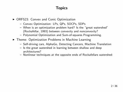
Topics
I ORF523 Convex and Conic Optimization
ndash Convex Optimization LPs QPs SOCPs SDPsndash When is an optimization problem hard Is the ldquogreat watershedrdquo
(Rockafellar 1993) between convexity and nonconvexityndash Polynomial Optimization and Sum-of-squares Programming
I Theme Optimization Problems in Machine Learning
ndash Self-driving cars AlphaGo Detecting Cancers Machine Translationndash Is the great watershed in learning between shallow and deep
architecturesndash Nonlinear techniques at the opposite ends of Rockafellars watershed
I Kernel Methods Convex Optimization Learning polynomialsI Random embeddings scalable kernel methods shallow networksI Deep Learning Nonconvex Optimization Architectures TensorFlow
ndash Some intriguing vignettes empirical observations open questionsI How expressive are Deep NetsI Why do Deep Nets generalizeI How hard is it to train Deep Nets
2 36
Setting
Estimate f X 7rarr Y from xiyili=1 sim p xi isin X yi isin Y
3 36
Setting
Estimate f X 7rarr Y from xiyili=1 sim p xi isin X yi isin Y
3 36
Regularized Loss Minimization
I Regularized Loss Minimization (GD SGD) in a suitable H
arg minfisinH
lsumi=1
V (f(xi)yi) + Ω(f)
I Understanding deep learning requires rethinking generalizationZhang et al 2017
4 36
Regularized Loss Minimization
I Regularized Loss Minimization (GD SGD) in a suitable H
arg minfisinH
lsumi=1
V (f(xi)yi) + Ω(f)
I Understanding deep learning requires rethinking generalizationZhang et al 2017
4 36
Optimization in Learning
I Optimal predictor
f = arg minf
E(xy)simpV (f(x)y)
I Approximation Error due to finite domain knowledge(Expressivity)
fH = arg minfisinH
E(xy)simpV (f(x)y)
I Estimation Error due to finite data (Generalization)
fH = arg minfisinH
lsumi=1
V (f(xi)yi) + Ω(f)
I Optimization Error finite computation (Optimization Landscape)
return f(i)H
Tractable but bad model or intractable but good model
5 36
Optimization in Learning
I Optimal predictor
f = arg minf
E(xy)simpV (f(x)y)
I Approximation Error due to finite domain knowledge(Expressivity)
fH = arg minfisinH
E(xy)simpV (f(x)y)
I Estimation Error due to finite data (Generalization)
fH = arg minfisinH
lsumi=1
V (f(xi)yi) + Ω(f)
I Optimization Error finite computation (Optimization Landscape)
return f(i)H
Tractable but bad model or intractable but good model 5 36
Nonlinearities Everywhere
Large l =rArr Big models H ldquorichrdquo non-parametricnonlinear
6 36
Nonlinearities Everywhere
Large l =rArr Big models H ldquorichrdquo non-parametricnonlinear
6 36
Nonlinearities Everywhere
Large l =rArr Big models H ldquorichrdquo non-parametricnonlinear
6 36
Choice of Nonlinear Hypothesis Space Kernels
x Ψ wTΨ(x) y
w
Ψ(x)
I eg Linear functions and Polynomials
I Infinite-dimensional nonlinear embeddings Fully non-parameteric
I Functional Analysis (Aronszajn Bergman (1950s)) Statistics (Parzen(1960s)) PDEs Numerical Analysis
I ML in 1990rsquos Nonlinear classification regression clustering time-seriesanalysis dynamical systems hypothesis testing causal modeling
I Convex Optimization
7 36
Choice of Nonlinear Hypothesis Space Kernels
x Ψ wTΨ(x) y
w
Ψ(x)
I eg Linear functions and Polynomials
I Infinite-dimensional nonlinear embeddings Fully non-parameteric
I Functional Analysis (Aronszajn Bergman (1950s)) Statistics (Parzen(1960s)) PDEs Numerical Analysis
I ML in 1990rsquos Nonlinear classification regression clustering time-seriesanalysis dynamical systems hypothesis testing causal modeling
I Convex Optimization
7 36
Choice of Nonlinear Hypothesis Space Kernels
x Ψ wTΨ(x) y
w
Ψ(x)
I eg Linear functions and Polynomials
I Infinite-dimensional nonlinear embeddings Fully non-parameteric
I Functional Analysis (Aronszajn Bergman (1950s)) Statistics (Parzen(1960s)) PDEs Numerical Analysis
I ML in 1990rsquos Nonlinear classification regression clustering time-seriesanalysis dynamical systems hypothesis testing causal modeling
I Convex Optimization
7 36
Choice of Nonlinear Hypothesis Space Kernels
x Ψ wTΨ(x) y
w
Ψ(x)
I eg Linear functions and Polynomials
I Infinite-dimensional nonlinear embeddings Fully non-parameteric
I Functional Analysis (Aronszajn Bergman (1950s)) Statistics (Parzen(1960s)) PDEs Numerical Analysis
I ML in 1990rsquos Nonlinear classification regression clustering time-seriesanalysis dynamical systems hypothesis testing causal modeling
I Convex Optimization
7 36
Choice of Nonlinear Hypothesis Space Kernels
x Ψ wTΨ(x) y
w
Ψ(x)
I eg Linear functions and Polynomials
I Infinite-dimensional nonlinear embeddings Fully non-parameteric
I Functional Analysis (Aronszajn Bergman (1950s)) Statistics (Parzen(1960s)) PDEs Numerical Analysis
I ML in 1990rsquos Nonlinear classification regression clustering time-seriesanalysis dynamical systems hypothesis testing causal modeling
I Convex Optimization
7 36
Choice of Nonlinear Hypothesis Space Deep Learning
x0 f1 f2 fL `
w1 w2 wL
z isin Rx1 x2 xLminus1 xL
I Compositions Raw data to higher abstractions (representation learning)
I Multilayer Perceptrons fl(xW) = σ(Wx) (sigmoids ReLU)I Turing (1950) In considering the functions of the mind or the brain we find certain operations which we can explain in
purely mechanical terms This we say does not correspond to the real mind it is a sort of skin which we must strip off if we are
to find the real mind Proceeding in this way do we ever come to the rdquorealrdquo mind or do we eventually come to the skin which
has nothing in it In the latter case the whole mind is mechanical
I Rosenblatt (1957) NYT 1958 New Navy Device Learns By Doing The Navy revealed the embryo of an electronic
computer today that it expects will be able to walk talk see write reproduce itself and be conscious of its existence Later
perceptrons will be able to recognize people and call out their names and instantly translate speech in one language to speech
and writing in another language it was predicted
I Perceptron (Minski and Pappert 1969) [Olarzan A Sociological Study 1996]I Backprop (1986) Reverse-mode differentiation (1960s-70s) CNNs (1980s 2012-)I Breadth-Width tradeoffsI Non-convex Optimization Domain-agnostic recipe
8 36
Choice of Nonlinear Hypothesis Space Deep Learning
x0 f1 f2 fL `
w1 w2 wL
z isin Rx1 x2 xLminus1 xL
I Compositions Raw data to higher abstractions (representation learning)I Multilayer Perceptrons fl(xW) = σ(Wx) (sigmoids ReLU)
I Turing (1950) In considering the functions of the mind or the brain we find certain operations which we can explain in
purely mechanical terms This we say does not correspond to the real mind it is a sort of skin which we must strip off if we are
to find the real mind Proceeding in this way do we ever come to the rdquorealrdquo mind or do we eventually come to the skin which
has nothing in it In the latter case the whole mind is mechanical
I Rosenblatt (1957) NYT 1958 New Navy Device Learns By Doing The Navy revealed the embryo of an electronic
computer today that it expects will be able to walk talk see write reproduce itself and be conscious of its existence Later
perceptrons will be able to recognize people and call out their names and instantly translate speech in one language to speech
and writing in another language it was predicted
I Perceptron (Minski and Pappert 1969) [Olarzan A Sociological Study 1996]I Backprop (1986) Reverse-mode differentiation (1960s-70s) CNNs (1980s 2012-)I Breadth-Width tradeoffsI Non-convex Optimization Domain-agnostic recipe
8 36
Choice of Nonlinear Hypothesis Space Deep Learning
x0 f1 f2 fL `
w1 w2 wL
z isin Rx1 x2 xLminus1 xL
I Compositions Raw data to higher abstractions (representation learning)I Multilayer Perceptrons fl(xW) = σ(Wx) (sigmoids ReLU)I Turing (1950) In considering the functions of the mind or the brain we find certain operations which we can explain in
purely mechanical terms This we say does not correspond to the real mind it is a sort of skin which we must strip off if we are
to find the real mind Proceeding in this way do we ever come to the rdquorealrdquo mind or do we eventually come to the skin which
has nothing in it In the latter case the whole mind is mechanical
I Rosenblatt (1957) NYT 1958 New Navy Device Learns By Doing The Navy revealed the embryo of an electronic
computer today that it expects will be able to walk talk see write reproduce itself and be conscious of its existence Later
perceptrons will be able to recognize people and call out their names and instantly translate speech in one language to speech
and writing in another language it was predicted
I Perceptron (Minski and Pappert 1969) [Olarzan A Sociological Study 1996]I Backprop (1986) Reverse-mode differentiation (1960s-70s) CNNs (1980s 2012-)I Breadth-Width tradeoffsI Non-convex Optimization Domain-agnostic recipe
8 36
Choice of Nonlinear Hypothesis Space Deep Learning
x0 f1 f2 fL `
w1 w2 wL
z isin Rx1 x2 xLminus1 xL
I Compositions Raw data to higher abstractions (representation learning)I Multilayer Perceptrons fl(xW) = σ(Wx) (sigmoids ReLU)I Turing (1950) In considering the functions of the mind or the brain we find certain operations which we can explain in
purely mechanical terms This we say does not correspond to the real mind it is a sort of skin which we must strip off if we are
to find the real mind Proceeding in this way do we ever come to the rdquorealrdquo mind or do we eventually come to the skin which
has nothing in it In the latter case the whole mind is mechanical
I Rosenblatt (1957) NYT 1958 New Navy Device Learns By Doing The Navy revealed the embryo of an electronic
computer today that it expects will be able to walk talk see write reproduce itself and be conscious of its existence Later
perceptrons will be able to recognize people and call out their names and instantly translate speech in one language to speech
and writing in another language it was predicted
I Perceptron (Minski and Pappert 1969) [Olarzan A Sociological Study 1996]I Backprop (1986) Reverse-mode differentiation (1960s-70s) CNNs (1980s 2012-)I Breadth-Width tradeoffsI Non-convex Optimization Domain-agnostic recipe
8 36
Choice of Nonlinear Hypothesis Space Deep Learning
x0 f1 f2 fL `
w1 w2 wL
z isin Rx1 x2 xLminus1 xL
I Compositions Raw data to higher abstractions (representation learning)I Multilayer Perceptrons fl(xW) = σ(Wx) (sigmoids ReLU)I Turing (1950) In considering the functions of the mind or the brain we find certain operations which we can explain in
purely mechanical terms This we say does not correspond to the real mind it is a sort of skin which we must strip off if we are
to find the real mind Proceeding in this way do we ever come to the rdquorealrdquo mind or do we eventually come to the skin which
has nothing in it In the latter case the whole mind is mechanical
I Rosenblatt (1957) NYT 1958 New Navy Device Learns By Doing The Navy revealed the embryo of an electronic
computer today that it expects will be able to walk talk see write reproduce itself and be conscious of its existence Later
perceptrons will be able to recognize people and call out their names and instantly translate speech in one language to speech
and writing in another language it was predicted
I Perceptron (Minski and Pappert 1969) [Olarzan A Sociological Study 1996]I Backprop (1986) Reverse-mode differentiation (1960s-70s) CNNs (1980s 2012-)
I Breadth-Width tradeoffsI Non-convex Optimization Domain-agnostic recipe
8 36
Choice of Nonlinear Hypothesis Space Deep Learning
x0 f1 f2 fL `
w1 w2 wL
z isin Rx1 x2 xLminus1 xL
I Compositions Raw data to higher abstractions (representation learning)I Multilayer Perceptrons fl(xW) = σ(Wx) (sigmoids ReLU)I Turing (1950) In considering the functions of the mind or the brain we find certain operations which we can explain in
purely mechanical terms This we say does not correspond to the real mind it is a sort of skin which we must strip off if we are
to find the real mind Proceeding in this way do we ever come to the rdquorealrdquo mind or do we eventually come to the skin which
has nothing in it In the latter case the whole mind is mechanical
I Rosenblatt (1957) NYT 1958 New Navy Device Learns By Doing The Navy revealed the embryo of an electronic
computer today that it expects will be able to walk talk see write reproduce itself and be conscious of its existence Later
perceptrons will be able to recognize people and call out their names and instantly translate speech in one language to speech
and writing in another language it was predicted
I Perceptron (Minski and Pappert 1969) [Olarzan A Sociological Study 1996]I Backprop (1986) Reverse-mode differentiation (1960s-70s) CNNs (1980s 2012-)I Breadth-Width tradeoffsI Non-convex Optimization Domain-agnostic recipe 8 36
Choice of Nonlinear Hypothesis Space Deep Learning
x0 f1 f2 fL `
w1 w2 wL
z isin Rx1 x2 xLminus1 xL
I Compositions Raw data to higher abstractions (representation learning)I Multilayer Perceptrons fl(xW) = σ(Wx) (sigmoids ReLU)I Turing (1950) In considering the functions of the mind or the brain we find certain operations which we can explain in
purely mechanical terms This we say does not correspond to the real mind it is a sort of skin which we must strip off if we are
to find the real mind Proceeding in this way do we ever come to the rdquorealrdquo mind or do we eventually come to the skin which
has nothing in it In the latter case the whole mind is mechanical
I Rosenblatt (1957) NYT 1958 New Navy Device Learns By Doing The Navy revealed the embryo of an electronic
computer today that it expects will be able to walk talk see write reproduce itself and be conscious of its existence Later
perceptrons will be able to recognize people and call out their names and instantly translate speech in one language to speech
and writing in another language it was predicted
I Perceptron (Minski and Pappert 1969) [Olarzan A Sociological Study 1996]I Backprop (1986) Reverse-mode differentiation (1960s-70s) CNNs (1980s 2012-)I Breadth-Width tradeoffsI Non-convex Optimization Domain-agnostic recipe 8 36
The Watershed Moment Imagenet 2012
I Many statistical and computational ingredientsndash Large datasets (ILSVRC since 2010)
ndash Large statistical capacity (12M images 60M params)ndash Distributed computationndash Depth Invariant feature learning (transferrable to other tasks)ndash Engineering Dropout ReLU
I Many astonishing results since then
9 36
The Watershed Moment Imagenet 2012
I Many statistical and computational ingredientsndash Large datasets (ILSVRC since 2010)ndash Large statistical capacity (12M images 60M params)
ndash Distributed computationndash Depth Invariant feature learning (transferrable to other tasks)ndash Engineering Dropout ReLU
I Many astonishing results since then
9 36
The Watershed Moment Imagenet 2012
I Many statistical and computational ingredientsndash Large datasets (ILSVRC since 2010)ndash Large statistical capacity (12M images 60M params)ndash Distributed computation
ndash Depth Invariant feature learning (transferrable to other tasks)ndash Engineering Dropout ReLU
I Many astonishing results since then
9 36
The Watershed Moment Imagenet 2012
I Many statistical and computational ingredientsndash Large datasets (ILSVRC since 2010)ndash Large statistical capacity (12M images 60M params)ndash Distributed computationndash Depth Invariant feature learning (transferrable to other tasks)
ndash Engineering Dropout ReLU I Many astonishing results since then
9 36
The Watershed Moment Imagenet 2012
I Many statistical and computational ingredientsndash Large datasets (ILSVRC since 2010)ndash Large statistical capacity (12M images 60M params)ndash Distributed computationndash Depth Invariant feature learning (transferrable to other tasks)ndash Engineering Dropout ReLU
I Many astonishing results since then
9 36
CNNs
10 36
Self-Driving Cars
Figure End-to-End Learning for Self-driving Cars Bojarski et al 2016
11 36
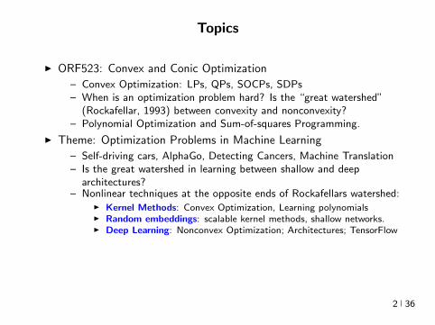
Topics
I ORF523 Convex and Conic Optimization
ndash Convex Optimization LPs QPs SOCPs SDPsndash When is an optimization problem hard Is the ldquogreat watershedrdquo
(Rockafellar 1993) between convexity and nonconvexityndash Polynomial Optimization and Sum-of-squares Programming
I Theme Optimization Problems in Machine Learning
ndash Self-driving cars AlphaGo Detecting Cancers Machine Translationndash Is the great watershed in learning between shallow and deep
architecturesndash Nonlinear techniques at the opposite ends of Rockafellars watershed
I Kernel Methods Convex Optimization Learning polynomialsI Random embeddings scalable kernel methods shallow networksI Deep Learning Nonconvex Optimization Architectures TensorFlow
ndash Some intriguing vignettes empirical observations open questionsI How expressive are Deep NetsI Why do Deep Nets generalizeI How hard is it to train Deep Nets
2 36
Topics
I ORF523 Convex and Conic Optimization
ndash Convex Optimization LPs QPs SOCPs SDPsndash When is an optimization problem hard Is the ldquogreat watershedrdquo
(Rockafellar 1993) between convexity and nonconvexityndash Polynomial Optimization and Sum-of-squares Programming
I Theme Optimization Problems in Machine Learning
ndash Self-driving cars AlphaGo Detecting Cancers Machine Translationndash Is the great watershed in learning between shallow and deep
architecturesndash Nonlinear techniques at the opposite ends of Rockafellars watershed
I Kernel Methods Convex Optimization Learning polynomialsI Random embeddings scalable kernel methods shallow networksI Deep Learning Nonconvex Optimization Architectures TensorFlow
ndash Some intriguing vignettes empirical observations open questionsI How expressive are Deep NetsI Why do Deep Nets generalizeI How hard is it to train Deep Nets
2 36
Setting
Estimate f X 7rarr Y from xiyili=1 sim p xi isin X yi isin Y
3 36
Setting
Estimate f X 7rarr Y from xiyili=1 sim p xi isin X yi isin Y
3 36
Regularized Loss Minimization
I Regularized Loss Minimization (GD SGD) in a suitable H
arg minfisinH
lsumi=1
V (f(xi)yi) + Ω(f)
I Understanding deep learning requires rethinking generalizationZhang et al 2017
4 36
Regularized Loss Minimization
I Regularized Loss Minimization (GD SGD) in a suitable H
arg minfisinH
lsumi=1
V (f(xi)yi) + Ω(f)
I Understanding deep learning requires rethinking generalizationZhang et al 2017
4 36
Optimization in Learning
I Optimal predictor
f = arg minf
E(xy)simpV (f(x)y)
I Approximation Error due to finite domain knowledge(Expressivity)
fH = arg minfisinH
E(xy)simpV (f(x)y)
I Estimation Error due to finite data (Generalization)
fH = arg minfisinH
lsumi=1
V (f(xi)yi) + Ω(f)
I Optimization Error finite computation (Optimization Landscape)
return f(i)H
Tractable but bad model or intractable but good model
5 36
Optimization in Learning
I Optimal predictor
f = arg minf
E(xy)simpV (f(x)y)
I Approximation Error due to finite domain knowledge(Expressivity)
fH = arg minfisinH
E(xy)simpV (f(x)y)
I Estimation Error due to finite data (Generalization)
fH = arg minfisinH
lsumi=1
V (f(xi)yi) + Ω(f)
I Optimization Error finite computation (Optimization Landscape)
return f(i)H
Tractable but bad model or intractable but good model 5 36
Nonlinearities Everywhere
Large l =rArr Big models H ldquorichrdquo non-parametricnonlinear
6 36
Nonlinearities Everywhere
Large l =rArr Big models H ldquorichrdquo non-parametricnonlinear
6 36
Nonlinearities Everywhere
Large l =rArr Big models H ldquorichrdquo non-parametricnonlinear
6 36
Choice of Nonlinear Hypothesis Space Kernels
x Ψ wTΨ(x) y
w
Ψ(x)
I eg Linear functions and Polynomials
I Infinite-dimensional nonlinear embeddings Fully non-parameteric
I Functional Analysis (Aronszajn Bergman (1950s)) Statistics (Parzen(1960s)) PDEs Numerical Analysis
I ML in 1990rsquos Nonlinear classification regression clustering time-seriesanalysis dynamical systems hypothesis testing causal modeling
I Convex Optimization
7 36
Choice of Nonlinear Hypothesis Space Kernels
x Ψ wTΨ(x) y
w
Ψ(x)
I eg Linear functions and Polynomials
I Infinite-dimensional nonlinear embeddings Fully non-parameteric
I Functional Analysis (Aronszajn Bergman (1950s)) Statistics (Parzen(1960s)) PDEs Numerical Analysis
I ML in 1990rsquos Nonlinear classification regression clustering time-seriesanalysis dynamical systems hypothesis testing causal modeling
I Convex Optimization
7 36
Choice of Nonlinear Hypothesis Space Kernels
x Ψ wTΨ(x) y
w
Ψ(x)
I eg Linear functions and Polynomials
I Infinite-dimensional nonlinear embeddings Fully non-parameteric
I Functional Analysis (Aronszajn Bergman (1950s)) Statistics (Parzen(1960s)) PDEs Numerical Analysis
I ML in 1990rsquos Nonlinear classification regression clustering time-seriesanalysis dynamical systems hypothesis testing causal modeling
I Convex Optimization
7 36
Choice of Nonlinear Hypothesis Space Kernels
x Ψ wTΨ(x) y
w
Ψ(x)
I eg Linear functions and Polynomials
I Infinite-dimensional nonlinear embeddings Fully non-parameteric
I Functional Analysis (Aronszajn Bergman (1950s)) Statistics (Parzen(1960s)) PDEs Numerical Analysis
I ML in 1990rsquos Nonlinear classification regression clustering time-seriesanalysis dynamical systems hypothesis testing causal modeling
I Convex Optimization
7 36
Choice of Nonlinear Hypothesis Space Kernels
x Ψ wTΨ(x) y
w
Ψ(x)
I eg Linear functions and Polynomials
I Infinite-dimensional nonlinear embeddings Fully non-parameteric
I Functional Analysis (Aronszajn Bergman (1950s)) Statistics (Parzen(1960s)) PDEs Numerical Analysis
I ML in 1990rsquos Nonlinear classification regression clustering time-seriesanalysis dynamical systems hypothesis testing causal modeling
I Convex Optimization
7 36
Choice of Nonlinear Hypothesis Space Deep Learning
x0 f1 f2 fL `
w1 w2 wL
z isin Rx1 x2 xLminus1 xL
I Compositions Raw data to higher abstractions (representation learning)
I Multilayer Perceptrons fl(xW) = σ(Wx) (sigmoids ReLU)I Turing (1950) In considering the functions of the mind or the brain we find certain operations which we can explain in
purely mechanical terms This we say does not correspond to the real mind it is a sort of skin which we must strip off if we are
to find the real mind Proceeding in this way do we ever come to the rdquorealrdquo mind or do we eventually come to the skin which
has nothing in it In the latter case the whole mind is mechanical
I Rosenblatt (1957) NYT 1958 New Navy Device Learns By Doing The Navy revealed the embryo of an electronic
computer today that it expects will be able to walk talk see write reproduce itself and be conscious of its existence Later
perceptrons will be able to recognize people and call out their names and instantly translate speech in one language to speech
and writing in another language it was predicted
I Perceptron (Minski and Pappert 1969) [Olarzan A Sociological Study 1996]I Backprop (1986) Reverse-mode differentiation (1960s-70s) CNNs (1980s 2012-)I Breadth-Width tradeoffsI Non-convex Optimization Domain-agnostic recipe
8 36
Choice of Nonlinear Hypothesis Space Deep Learning
x0 f1 f2 fL `
w1 w2 wL
z isin Rx1 x2 xLminus1 xL
I Compositions Raw data to higher abstractions (representation learning)I Multilayer Perceptrons fl(xW) = σ(Wx) (sigmoids ReLU)
I Turing (1950) In considering the functions of the mind or the brain we find certain operations which we can explain in
purely mechanical terms This we say does not correspond to the real mind it is a sort of skin which we must strip off if we are
to find the real mind Proceeding in this way do we ever come to the rdquorealrdquo mind or do we eventually come to the skin which
has nothing in it In the latter case the whole mind is mechanical
I Rosenblatt (1957) NYT 1958 New Navy Device Learns By Doing The Navy revealed the embryo of an electronic
computer today that it expects will be able to walk talk see write reproduce itself and be conscious of its existence Later
perceptrons will be able to recognize people and call out their names and instantly translate speech in one language to speech
and writing in another language it was predicted
I Perceptron (Minski and Pappert 1969) [Olarzan A Sociological Study 1996]I Backprop (1986) Reverse-mode differentiation (1960s-70s) CNNs (1980s 2012-)I Breadth-Width tradeoffsI Non-convex Optimization Domain-agnostic recipe
8 36
Choice of Nonlinear Hypothesis Space Deep Learning
x0 f1 f2 fL `
w1 w2 wL
z isin Rx1 x2 xLminus1 xL
I Compositions Raw data to higher abstractions (representation learning)I Multilayer Perceptrons fl(xW) = σ(Wx) (sigmoids ReLU)I Turing (1950) In considering the functions of the mind or the brain we find certain operations which we can explain in
purely mechanical terms This we say does not correspond to the real mind it is a sort of skin which we must strip off if we are
to find the real mind Proceeding in this way do we ever come to the rdquorealrdquo mind or do we eventually come to the skin which
has nothing in it In the latter case the whole mind is mechanical
I Rosenblatt (1957) NYT 1958 New Navy Device Learns By Doing The Navy revealed the embryo of an electronic
computer today that it expects will be able to walk talk see write reproduce itself and be conscious of its existence Later
perceptrons will be able to recognize people and call out their names and instantly translate speech in one language to speech
and writing in another language it was predicted
I Perceptron (Minski and Pappert 1969) [Olarzan A Sociological Study 1996]I Backprop (1986) Reverse-mode differentiation (1960s-70s) CNNs (1980s 2012-)I Breadth-Width tradeoffsI Non-convex Optimization Domain-agnostic recipe
8 36
Choice of Nonlinear Hypothesis Space Deep Learning
x0 f1 f2 fL `
w1 w2 wL
z isin Rx1 x2 xLminus1 xL
I Compositions Raw data to higher abstractions (representation learning)I Multilayer Perceptrons fl(xW) = σ(Wx) (sigmoids ReLU)I Turing (1950) In considering the functions of the mind or the brain we find certain operations which we can explain in
purely mechanical terms This we say does not correspond to the real mind it is a sort of skin which we must strip off if we are
to find the real mind Proceeding in this way do we ever come to the rdquorealrdquo mind or do we eventually come to the skin which
has nothing in it In the latter case the whole mind is mechanical
I Rosenblatt (1957) NYT 1958 New Navy Device Learns By Doing The Navy revealed the embryo of an electronic
computer today that it expects will be able to walk talk see write reproduce itself and be conscious of its existence Later
perceptrons will be able to recognize people and call out their names and instantly translate speech in one language to speech
and writing in another language it was predicted
I Perceptron (Minski and Pappert 1969) [Olarzan A Sociological Study 1996]I Backprop (1986) Reverse-mode differentiation (1960s-70s) CNNs (1980s 2012-)I Breadth-Width tradeoffsI Non-convex Optimization Domain-agnostic recipe
8 36
Choice of Nonlinear Hypothesis Space Deep Learning
x0 f1 f2 fL `
w1 w2 wL
z isin Rx1 x2 xLminus1 xL
I Compositions Raw data to higher abstractions (representation learning)I Multilayer Perceptrons fl(xW) = σ(Wx) (sigmoids ReLU)I Turing (1950) In considering the functions of the mind or the brain we find certain operations which we can explain in
purely mechanical terms This we say does not correspond to the real mind it is a sort of skin which we must strip off if we are
to find the real mind Proceeding in this way do we ever come to the rdquorealrdquo mind or do we eventually come to the skin which
has nothing in it In the latter case the whole mind is mechanical
I Rosenblatt (1957) NYT 1958 New Navy Device Learns By Doing The Navy revealed the embryo of an electronic
computer today that it expects will be able to walk talk see write reproduce itself and be conscious of its existence Later
perceptrons will be able to recognize people and call out their names and instantly translate speech in one language to speech
and writing in another language it was predicted
I Perceptron (Minski and Pappert 1969) [Olarzan A Sociological Study 1996]I Backprop (1986) Reverse-mode differentiation (1960s-70s) CNNs (1980s 2012-)
I Breadth-Width tradeoffsI Non-convex Optimization Domain-agnostic recipe
8 36
Choice of Nonlinear Hypothesis Space Deep Learning
x0 f1 f2 fL `
w1 w2 wL
z isin Rx1 x2 xLminus1 xL
I Compositions Raw data to higher abstractions (representation learning)I Multilayer Perceptrons fl(xW) = σ(Wx) (sigmoids ReLU)I Turing (1950) In considering the functions of the mind or the brain we find certain operations which we can explain in
purely mechanical terms This we say does not correspond to the real mind it is a sort of skin which we must strip off if we are
to find the real mind Proceeding in this way do we ever come to the rdquorealrdquo mind or do we eventually come to the skin which
has nothing in it In the latter case the whole mind is mechanical
I Rosenblatt (1957) NYT 1958 New Navy Device Learns By Doing The Navy revealed the embryo of an electronic
computer today that it expects will be able to walk talk see write reproduce itself and be conscious of its existence Later
perceptrons will be able to recognize people and call out their names and instantly translate speech in one language to speech
and writing in another language it was predicted
I Perceptron (Minski and Pappert 1969) [Olarzan A Sociological Study 1996]I Backprop (1986) Reverse-mode differentiation (1960s-70s) CNNs (1980s 2012-)I Breadth-Width tradeoffsI Non-convex Optimization Domain-agnostic recipe 8 36
Choice of Nonlinear Hypothesis Space Deep Learning
x0 f1 f2 fL `
w1 w2 wL
z isin Rx1 x2 xLminus1 xL
I Compositions Raw data to higher abstractions (representation learning)I Multilayer Perceptrons fl(xW) = σ(Wx) (sigmoids ReLU)I Turing (1950) In considering the functions of the mind or the brain we find certain operations which we can explain in
purely mechanical terms This we say does not correspond to the real mind it is a sort of skin which we must strip off if we are
to find the real mind Proceeding in this way do we ever come to the rdquorealrdquo mind or do we eventually come to the skin which
has nothing in it In the latter case the whole mind is mechanical
I Rosenblatt (1957) NYT 1958 New Navy Device Learns By Doing The Navy revealed the embryo of an electronic
computer today that it expects will be able to walk talk see write reproduce itself and be conscious of its existence Later
perceptrons will be able to recognize people and call out their names and instantly translate speech in one language to speech
and writing in another language it was predicted
I Perceptron (Minski and Pappert 1969) [Olarzan A Sociological Study 1996]I Backprop (1986) Reverse-mode differentiation (1960s-70s) CNNs (1980s 2012-)I Breadth-Width tradeoffsI Non-convex Optimization Domain-agnostic recipe 8 36
The Watershed Moment Imagenet 2012
I Many statistical and computational ingredientsndash Large datasets (ILSVRC since 2010)
ndash Large statistical capacity (12M images 60M params)ndash Distributed computationndash Depth Invariant feature learning (transferrable to other tasks)ndash Engineering Dropout ReLU
I Many astonishing results since then
9 36
The Watershed Moment Imagenet 2012
I Many statistical and computational ingredientsndash Large datasets (ILSVRC since 2010)ndash Large statistical capacity (12M images 60M params)
ndash Distributed computationndash Depth Invariant feature learning (transferrable to other tasks)ndash Engineering Dropout ReLU
I Many astonishing results since then
9 36
The Watershed Moment Imagenet 2012
I Many statistical and computational ingredientsndash Large datasets (ILSVRC since 2010)ndash Large statistical capacity (12M images 60M params)ndash Distributed computation
ndash Depth Invariant feature learning (transferrable to other tasks)ndash Engineering Dropout ReLU
I Many astonishing results since then
9 36
The Watershed Moment Imagenet 2012
I Many statistical and computational ingredientsndash Large datasets (ILSVRC since 2010)ndash Large statistical capacity (12M images 60M params)ndash Distributed computationndash Depth Invariant feature learning (transferrable to other tasks)
ndash Engineering Dropout ReLU I Many astonishing results since then
9 36
The Watershed Moment Imagenet 2012
I Many statistical and computational ingredientsndash Large datasets (ILSVRC since 2010)ndash Large statistical capacity (12M images 60M params)ndash Distributed computationndash Depth Invariant feature learning (transferrable to other tasks)ndash Engineering Dropout ReLU
I Many astonishing results since then
9 36
CNNs
10 36
Self-Driving Cars
Figure End-to-End Learning for Self-driving Cars Bojarski et al 2016
11 36

Topics
I ORF523 Convex and Conic Optimization
ndash Convex Optimization LPs QPs SOCPs SDPsndash When is an optimization problem hard Is the ldquogreat watershedrdquo
(Rockafellar 1993) between convexity and nonconvexityndash Polynomial Optimization and Sum-of-squares Programming
I Theme Optimization Problems in Machine Learning
ndash Self-driving cars AlphaGo Detecting Cancers Machine Translationndash Is the great watershed in learning between shallow and deep
architecturesndash Nonlinear techniques at the opposite ends of Rockafellars watershed
I Kernel Methods Convex Optimization Learning polynomialsI Random embeddings scalable kernel methods shallow networksI Deep Learning Nonconvex Optimization Architectures TensorFlow
ndash Some intriguing vignettes empirical observations open questionsI How expressive are Deep NetsI Why do Deep Nets generalizeI How hard is it to train Deep Nets
2 36
Setting
Estimate f X 7rarr Y from xiyili=1 sim p xi isin X yi isin Y
3 36
Setting
Estimate f X 7rarr Y from xiyili=1 sim p xi isin X yi isin Y
3 36
Regularized Loss Minimization
I Regularized Loss Minimization (GD SGD) in a suitable H
arg minfisinH
lsumi=1
V (f(xi)yi) + Ω(f)
I Understanding deep learning requires rethinking generalizationZhang et al 2017
4 36
Regularized Loss Minimization
I Regularized Loss Minimization (GD SGD) in a suitable H
arg minfisinH
lsumi=1
V (f(xi)yi) + Ω(f)
I Understanding deep learning requires rethinking generalizationZhang et al 2017
4 36
Optimization in Learning
I Optimal predictor
f = arg minf
E(xy)simpV (f(x)y)
I Approximation Error due to finite domain knowledge(Expressivity)
fH = arg minfisinH
E(xy)simpV (f(x)y)
I Estimation Error due to finite data (Generalization)
fH = arg minfisinH
lsumi=1
V (f(xi)yi) + Ω(f)
I Optimization Error finite computation (Optimization Landscape)
return f(i)H
Tractable but bad model or intractable but good model
5 36
Optimization in Learning
I Optimal predictor
f = arg minf
E(xy)simpV (f(x)y)
I Approximation Error due to finite domain knowledge(Expressivity)
fH = arg minfisinH
E(xy)simpV (f(x)y)
I Estimation Error due to finite data (Generalization)
fH = arg minfisinH
lsumi=1
V (f(xi)yi) + Ω(f)
I Optimization Error finite computation (Optimization Landscape)
return f(i)H
Tractable but bad model or intractable but good model 5 36
Nonlinearities Everywhere
Large l =rArr Big models H ldquorichrdquo non-parametricnonlinear
6 36
Nonlinearities Everywhere
Large l =rArr Big models H ldquorichrdquo non-parametricnonlinear
6 36
Nonlinearities Everywhere
Large l =rArr Big models H ldquorichrdquo non-parametricnonlinear
6 36
Choice of Nonlinear Hypothesis Space Kernels
x Ψ wTΨ(x) y
w
Ψ(x)
I eg Linear functions and Polynomials
I Infinite-dimensional nonlinear embeddings Fully non-parameteric
I Functional Analysis (Aronszajn Bergman (1950s)) Statistics (Parzen(1960s)) PDEs Numerical Analysis
I ML in 1990rsquos Nonlinear classification regression clustering time-seriesanalysis dynamical systems hypothesis testing causal modeling
I Convex Optimization
7 36
Choice of Nonlinear Hypothesis Space Kernels
x Ψ wTΨ(x) y
w
Ψ(x)
I eg Linear functions and Polynomials
I Infinite-dimensional nonlinear embeddings Fully non-parameteric
I Functional Analysis (Aronszajn Bergman (1950s)) Statistics (Parzen(1960s)) PDEs Numerical Analysis
I ML in 1990rsquos Nonlinear classification regression clustering time-seriesanalysis dynamical systems hypothesis testing causal modeling
I Convex Optimization
7 36
Choice of Nonlinear Hypothesis Space Kernels
x Ψ wTΨ(x) y
w
Ψ(x)
I eg Linear functions and Polynomials
I Infinite-dimensional nonlinear embeddings Fully non-parameteric
I Functional Analysis (Aronszajn Bergman (1950s)) Statistics (Parzen(1960s)) PDEs Numerical Analysis
I ML in 1990rsquos Nonlinear classification regression clustering time-seriesanalysis dynamical systems hypothesis testing causal modeling
I Convex Optimization
7 36
Choice of Nonlinear Hypothesis Space Kernels
x Ψ wTΨ(x) y
w
Ψ(x)
I eg Linear functions and Polynomials
I Infinite-dimensional nonlinear embeddings Fully non-parameteric
I Functional Analysis (Aronszajn Bergman (1950s)) Statistics (Parzen(1960s)) PDEs Numerical Analysis
I ML in 1990rsquos Nonlinear classification regression clustering time-seriesanalysis dynamical systems hypothesis testing causal modeling
I Convex Optimization
7 36
Choice of Nonlinear Hypothesis Space Kernels
x Ψ wTΨ(x) y
w
Ψ(x)
I eg Linear functions and Polynomials
I Infinite-dimensional nonlinear embeddings Fully non-parameteric
I Functional Analysis (Aronszajn Bergman (1950s)) Statistics (Parzen(1960s)) PDEs Numerical Analysis
I ML in 1990rsquos Nonlinear classification regression clustering time-seriesanalysis dynamical systems hypothesis testing causal modeling
I Convex Optimization
7 36
Choice of Nonlinear Hypothesis Space Deep Learning
x0 f1 f2 fL `
w1 w2 wL
z isin Rx1 x2 xLminus1 xL
I Compositions Raw data to higher abstractions (representation learning)
I Multilayer Perceptrons fl(xW) = σ(Wx) (sigmoids ReLU)I Turing (1950) In considering the functions of the mind or the brain we find certain operations which we can explain in
purely mechanical terms This we say does not correspond to the real mind it is a sort of skin which we must strip off if we are
to find the real mind Proceeding in this way do we ever come to the rdquorealrdquo mind or do we eventually come to the skin which
has nothing in it In the latter case the whole mind is mechanical
I Rosenblatt (1957) NYT 1958 New Navy Device Learns By Doing The Navy revealed the embryo of an electronic
computer today that it expects will be able to walk talk see write reproduce itself and be conscious of its existence Later
perceptrons will be able to recognize people and call out their names and instantly translate speech in one language to speech
and writing in another language it was predicted
I Perceptron (Minski and Pappert 1969) [Olarzan A Sociological Study 1996]I Backprop (1986) Reverse-mode differentiation (1960s-70s) CNNs (1980s 2012-)I Breadth-Width tradeoffsI Non-convex Optimization Domain-agnostic recipe
8 36
Choice of Nonlinear Hypothesis Space Deep Learning
x0 f1 f2 fL `
w1 w2 wL
z isin Rx1 x2 xLminus1 xL
I Compositions Raw data to higher abstractions (representation learning)I Multilayer Perceptrons fl(xW) = σ(Wx) (sigmoids ReLU)
I Turing (1950) In considering the functions of the mind or the brain we find certain operations which we can explain in
purely mechanical terms This we say does not correspond to the real mind it is a sort of skin which we must strip off if we are
to find the real mind Proceeding in this way do we ever come to the rdquorealrdquo mind or do we eventually come to the skin which
has nothing in it In the latter case the whole mind is mechanical
I Rosenblatt (1957) NYT 1958 New Navy Device Learns By Doing The Navy revealed the embryo of an electronic
computer today that it expects will be able to walk talk see write reproduce itself and be conscious of its existence Later
perceptrons will be able to recognize people and call out their names and instantly translate speech in one language to speech
and writing in another language it was predicted
I Perceptron (Minski and Pappert 1969) [Olarzan A Sociological Study 1996]I Backprop (1986) Reverse-mode differentiation (1960s-70s) CNNs (1980s 2012-)I Breadth-Width tradeoffsI Non-convex Optimization Domain-agnostic recipe
8 36
Choice of Nonlinear Hypothesis Space Deep Learning
x0 f1 f2 fL `
w1 w2 wL
z isin Rx1 x2 xLminus1 xL
I Compositions Raw data to higher abstractions (representation learning)I Multilayer Perceptrons fl(xW) = σ(Wx) (sigmoids ReLU)I Turing (1950) In considering the functions of the mind or the brain we find certain operations which we can explain in
purely mechanical terms This we say does not correspond to the real mind it is a sort of skin which we must strip off if we are
to find the real mind Proceeding in this way do we ever come to the rdquorealrdquo mind or do we eventually come to the skin which
has nothing in it In the latter case the whole mind is mechanical
I Rosenblatt (1957) NYT 1958 New Navy Device Learns By Doing The Navy revealed the embryo of an electronic
computer today that it expects will be able to walk talk see write reproduce itself and be conscious of its existence Later
perceptrons will be able to recognize people and call out their names and instantly translate speech in one language to speech
and writing in another language it was predicted
I Perceptron (Minski and Pappert 1969) [Olarzan A Sociological Study 1996]I Backprop (1986) Reverse-mode differentiation (1960s-70s) CNNs (1980s 2012-)I Breadth-Width tradeoffsI Non-convex Optimization Domain-agnostic recipe
8 36
Choice of Nonlinear Hypothesis Space Deep Learning
x0 f1 f2 fL `
w1 w2 wL
z isin Rx1 x2 xLminus1 xL
I Compositions Raw data to higher abstractions (representation learning)I Multilayer Perceptrons fl(xW) = σ(Wx) (sigmoids ReLU)I Turing (1950) In considering the functions of the mind or the brain we find certain operations which we can explain in
purely mechanical terms This we say does not correspond to the real mind it is a sort of skin which we must strip off if we are
to find the real mind Proceeding in this way do we ever come to the rdquorealrdquo mind or do we eventually come to the skin which
has nothing in it In the latter case the whole mind is mechanical
I Rosenblatt (1957) NYT 1958 New Navy Device Learns By Doing The Navy revealed the embryo of an electronic
computer today that it expects will be able to walk talk see write reproduce itself and be conscious of its existence Later
perceptrons will be able to recognize people and call out their names and instantly translate speech in one language to speech
and writing in another language it was predicted
I Perceptron (Minski and Pappert 1969) [Olarzan A Sociological Study 1996]I Backprop (1986) Reverse-mode differentiation (1960s-70s) CNNs (1980s 2012-)I Breadth-Width tradeoffsI Non-convex Optimization Domain-agnostic recipe
8 36
Choice of Nonlinear Hypothesis Space Deep Learning
x0 f1 f2 fL `
w1 w2 wL
z isin Rx1 x2 xLminus1 xL
I Compositions Raw data to higher abstractions (representation learning)I Multilayer Perceptrons fl(xW) = σ(Wx) (sigmoids ReLU)I Turing (1950) In considering the functions of the mind or the brain we find certain operations which we can explain in
purely mechanical terms This we say does not correspond to the real mind it is a sort of skin which we must strip off if we are
to find the real mind Proceeding in this way do we ever come to the rdquorealrdquo mind or do we eventually come to the skin which
has nothing in it In the latter case the whole mind is mechanical
I Rosenblatt (1957) NYT 1958 New Navy Device Learns By Doing The Navy revealed the embryo of an electronic
computer today that it expects will be able to walk talk see write reproduce itself and be conscious of its existence Later
perceptrons will be able to recognize people and call out their names and instantly translate speech in one language to speech
and writing in another language it was predicted
I Perceptron (Minski and Pappert 1969) [Olarzan A Sociological Study 1996]I Backprop (1986) Reverse-mode differentiation (1960s-70s) CNNs (1980s 2012-)
I Breadth-Width tradeoffsI Non-convex Optimization Domain-agnostic recipe
8 36
Choice of Nonlinear Hypothesis Space Deep Learning
x0 f1 f2 fL `
w1 w2 wL
z isin Rx1 x2 xLminus1 xL
I Compositions Raw data to higher abstractions (representation learning)I Multilayer Perceptrons fl(xW) = σ(Wx) (sigmoids ReLU)I Turing (1950) In considering the functions of the mind or the brain we find certain operations which we can explain in
purely mechanical terms This we say does not correspond to the real mind it is a sort of skin which we must strip off if we are
to find the real mind Proceeding in this way do we ever come to the rdquorealrdquo mind or do we eventually come to the skin which
has nothing in it In the latter case the whole mind is mechanical
I Rosenblatt (1957) NYT 1958 New Navy Device Learns By Doing The Navy revealed the embryo of an electronic
computer today that it expects will be able to walk talk see write reproduce itself and be conscious of its existence Later
perceptrons will be able to recognize people and call out their names and instantly translate speech in one language to speech
and writing in another language it was predicted
I Perceptron (Minski and Pappert 1969) [Olarzan A Sociological Study 1996]I Backprop (1986) Reverse-mode differentiation (1960s-70s) CNNs (1980s 2012-)I Breadth-Width tradeoffsI Non-convex Optimization Domain-agnostic recipe 8 36
Choice of Nonlinear Hypothesis Space Deep Learning
x0 f1 f2 fL `
w1 w2 wL
z isin Rx1 x2 xLminus1 xL
I Compositions Raw data to higher abstractions (representation learning)I Multilayer Perceptrons fl(xW) = σ(Wx) (sigmoids ReLU)I Turing (1950) In considering the functions of the mind or the brain we find certain operations which we can explain in
purely mechanical terms This we say does not correspond to the real mind it is a sort of skin which we must strip off if we are
to find the real mind Proceeding in this way do we ever come to the rdquorealrdquo mind or do we eventually come to the skin which
has nothing in it In the latter case the whole mind is mechanical
I Rosenblatt (1957) NYT 1958 New Navy Device Learns By Doing The Navy revealed the embryo of an electronic
computer today that it expects will be able to walk talk see write reproduce itself and be conscious of its existence Later
perceptrons will be able to recognize people and call out their names and instantly translate speech in one language to speech
and writing in another language it was predicted
I Perceptron (Minski and Pappert 1969) [Olarzan A Sociological Study 1996]I Backprop (1986) Reverse-mode differentiation (1960s-70s) CNNs (1980s 2012-)I Breadth-Width tradeoffsI Non-convex Optimization Domain-agnostic recipe 8 36
The Watershed Moment Imagenet 2012
I Many statistical and computational ingredientsndash Large datasets (ILSVRC since 2010)
ndash Large statistical capacity (12M images 60M params)ndash Distributed computationndash Depth Invariant feature learning (transferrable to other tasks)ndash Engineering Dropout ReLU
I Many astonishing results since then
9 36
The Watershed Moment Imagenet 2012
I Many statistical and computational ingredientsndash Large datasets (ILSVRC since 2010)ndash Large statistical capacity (12M images 60M params)
ndash Distributed computationndash Depth Invariant feature learning (transferrable to other tasks)ndash Engineering Dropout ReLU
I Many astonishing results since then
9 36
The Watershed Moment Imagenet 2012
I Many statistical and computational ingredientsndash Large datasets (ILSVRC since 2010)ndash Large statistical capacity (12M images 60M params)ndash Distributed computation
ndash Depth Invariant feature learning (transferrable to other tasks)ndash Engineering Dropout ReLU
I Many astonishing results since then
9 36
The Watershed Moment Imagenet 2012
I Many statistical and computational ingredientsndash Large datasets (ILSVRC since 2010)ndash Large statistical capacity (12M images 60M params)ndash Distributed computationndash Depth Invariant feature learning (transferrable to other tasks)
ndash Engineering Dropout ReLU I Many astonishing results since then
9 36
The Watershed Moment Imagenet 2012
I Many statistical and computational ingredientsndash Large datasets (ILSVRC since 2010)ndash Large statistical capacity (12M images 60M params)ndash Distributed computationndash Depth Invariant feature learning (transferrable to other tasks)ndash Engineering Dropout ReLU
I Many astonishing results since then
9 36
CNNs
10 36
Self-Driving Cars
Figure End-to-End Learning for Self-driving Cars Bojarski et al 2016
11 36
Setting
Estimate f X 7rarr Y from xiyili=1 sim p xi isin X yi isin Y
3 36
Setting
Estimate f X 7rarr Y from xiyili=1 sim p xi isin X yi isin Y
3 36
Regularized Loss Minimization
I Regularized Loss Minimization (GD SGD) in a suitable H
arg minfisinH
lsumi=1
V (f(xi)yi) + Ω(f)
I Understanding deep learning requires rethinking generalizationZhang et al 2017
4 36
Regularized Loss Minimization
I Regularized Loss Minimization (GD SGD) in a suitable H
arg minfisinH
lsumi=1
V (f(xi)yi) + Ω(f)
I Understanding deep learning requires rethinking generalizationZhang et al 2017
4 36
Optimization in Learning
I Optimal predictor
f = arg minf
E(xy)simpV (f(x)y)
I Approximation Error due to finite domain knowledge(Expressivity)
fH = arg minfisinH
E(xy)simpV (f(x)y)
I Estimation Error due to finite data (Generalization)
fH = arg minfisinH
lsumi=1
V (f(xi)yi) + Ω(f)
I Optimization Error finite computation (Optimization Landscape)
return f(i)H
Tractable but bad model or intractable but good model
5 36
Optimization in Learning
I Optimal predictor
f = arg minf
E(xy)simpV (f(x)y)
I Approximation Error due to finite domain knowledge(Expressivity)
fH = arg minfisinH
E(xy)simpV (f(x)y)
I Estimation Error due to finite data (Generalization)
fH = arg minfisinH
lsumi=1
V (f(xi)yi) + Ω(f)
I Optimization Error finite computation (Optimization Landscape)
return f(i)H
Tractable but bad model or intractable but good model 5 36
Nonlinearities Everywhere
Large l =rArr Big models H ldquorichrdquo non-parametricnonlinear
6 36
Nonlinearities Everywhere
Large l =rArr Big models H ldquorichrdquo non-parametricnonlinear
6 36
Nonlinearities Everywhere
Large l =rArr Big models H ldquorichrdquo non-parametricnonlinear
6 36
Choice of Nonlinear Hypothesis Space Kernels
x Ψ wTΨ(x) y
w
Ψ(x)
I eg Linear functions and Polynomials
I Infinite-dimensional nonlinear embeddings Fully non-parameteric
I Functional Analysis (Aronszajn Bergman (1950s)) Statistics (Parzen(1960s)) PDEs Numerical Analysis
I ML in 1990rsquos Nonlinear classification regression clustering time-seriesanalysis dynamical systems hypothesis testing causal modeling
I Convex Optimization
7 36
Choice of Nonlinear Hypothesis Space Kernels
x Ψ wTΨ(x) y
w
Ψ(x)
I eg Linear functions and Polynomials
I Infinite-dimensional nonlinear embeddings Fully non-parameteric
I Functional Analysis (Aronszajn Bergman (1950s)) Statistics (Parzen(1960s)) PDEs Numerical Analysis
I ML in 1990rsquos Nonlinear classification regression clustering time-seriesanalysis dynamical systems hypothesis testing causal modeling
I Convex Optimization
7 36
Choice of Nonlinear Hypothesis Space Kernels
x Ψ wTΨ(x) y
w
Ψ(x)
I eg Linear functions and Polynomials
I Infinite-dimensional nonlinear embeddings Fully non-parameteric
I Functional Analysis (Aronszajn Bergman (1950s)) Statistics (Parzen(1960s)) PDEs Numerical Analysis
I ML in 1990rsquos Nonlinear classification regression clustering time-seriesanalysis dynamical systems hypothesis testing causal modeling
I Convex Optimization
7 36
Choice of Nonlinear Hypothesis Space Kernels
x Ψ wTΨ(x) y
w
Ψ(x)
I eg Linear functions and Polynomials
I Infinite-dimensional nonlinear embeddings Fully non-parameteric
I Functional Analysis (Aronszajn Bergman (1950s)) Statistics (Parzen(1960s)) PDEs Numerical Analysis
I ML in 1990rsquos Nonlinear classification regression clustering time-seriesanalysis dynamical systems hypothesis testing causal modeling
I Convex Optimization
7 36
Choice of Nonlinear Hypothesis Space Kernels
x Ψ wTΨ(x) y
w
Ψ(x)
I eg Linear functions and Polynomials
I Infinite-dimensional nonlinear embeddings Fully non-parameteric
I Functional Analysis (Aronszajn Bergman (1950s)) Statistics (Parzen(1960s)) PDEs Numerical Analysis
I ML in 1990rsquos Nonlinear classification regression clustering time-seriesanalysis dynamical systems hypothesis testing causal modeling
I Convex Optimization
7 36
Choice of Nonlinear Hypothesis Space Deep Learning
x0 f1 f2 fL `
w1 w2 wL
z isin Rx1 x2 xLminus1 xL
I Compositions Raw data to higher abstractions (representation learning)
I Multilayer Perceptrons fl(xW) = σ(Wx) (sigmoids ReLU)I Turing (1950) In considering the functions of the mind or the brain we find certain operations which we can explain in
purely mechanical terms This we say does not correspond to the real mind it is a sort of skin which we must strip off if we are
to find the real mind Proceeding in this way do we ever come to the rdquorealrdquo mind or do we eventually come to the skin which
has nothing in it In the latter case the whole mind is mechanical
I Rosenblatt (1957) NYT 1958 New Navy Device Learns By Doing The Navy revealed the embryo of an electronic
computer today that it expects will be able to walk talk see write reproduce itself and be conscious of its existence Later
perceptrons will be able to recognize people and call out their names and instantly translate speech in one language to speech
and writing in another language it was predicted
I Perceptron (Minski and Pappert 1969) [Olarzan A Sociological Study 1996]I Backprop (1986) Reverse-mode differentiation (1960s-70s) CNNs (1980s 2012-)I Breadth-Width tradeoffsI Non-convex Optimization Domain-agnostic recipe
8 36
Choice of Nonlinear Hypothesis Space Deep Learning
x0 f1 f2 fL `
w1 w2 wL
z isin Rx1 x2 xLminus1 xL
I Compositions Raw data to higher abstractions (representation learning)I Multilayer Perceptrons fl(xW) = σ(Wx) (sigmoids ReLU)
I Turing (1950) In considering the functions of the mind or the brain we find certain operations which we can explain in
purely mechanical terms This we say does not correspond to the real mind it is a sort of skin which we must strip off if we are
to find the real mind Proceeding in this way do we ever come to the rdquorealrdquo mind or do we eventually come to the skin which
has nothing in it In the latter case the whole mind is mechanical
I Rosenblatt (1957) NYT 1958 New Navy Device Learns By Doing The Navy revealed the embryo of an electronic
computer today that it expects will be able to walk talk see write reproduce itself and be conscious of its existence Later
perceptrons will be able to recognize people and call out their names and instantly translate speech in one language to speech
and writing in another language it was predicted
I Perceptron (Minski and Pappert 1969) [Olarzan A Sociological Study 1996]I Backprop (1986) Reverse-mode differentiation (1960s-70s) CNNs (1980s 2012-)I Breadth-Width tradeoffsI Non-convex Optimization Domain-agnostic recipe
8 36
Choice of Nonlinear Hypothesis Space Deep Learning
x0 f1 f2 fL `
w1 w2 wL
z isin Rx1 x2 xLminus1 xL
I Compositions Raw data to higher abstractions (representation learning)I Multilayer Perceptrons fl(xW) = σ(Wx) (sigmoids ReLU)I Turing (1950) In considering the functions of the mind or the brain we find certain operations which we can explain in
purely mechanical terms This we say does not correspond to the real mind it is a sort of skin which we must strip off if we are
to find the real mind Proceeding in this way do we ever come to the rdquorealrdquo mind or do we eventually come to the skin which
has nothing in it In the latter case the whole mind is mechanical
I Rosenblatt (1957) NYT 1958 New Navy Device Learns By Doing The Navy revealed the embryo of an electronic
computer today that it expects will be able to walk talk see write reproduce itself and be conscious of its existence Later
perceptrons will be able to recognize people and call out their names and instantly translate speech in one language to speech
and writing in another language it was predicted
I Perceptron (Minski and Pappert 1969) [Olarzan A Sociological Study 1996]I Backprop (1986) Reverse-mode differentiation (1960s-70s) CNNs (1980s 2012-)I Breadth-Width tradeoffsI Non-convex Optimization Domain-agnostic recipe
8 36
Choice of Nonlinear Hypothesis Space Deep Learning
x0 f1 f2 fL `
w1 w2 wL
z isin Rx1 x2 xLminus1 xL
I Compositions Raw data to higher abstractions (representation learning)I Multilayer Perceptrons fl(xW) = σ(Wx) (sigmoids ReLU)I Turing (1950) In considering the functions of the mind or the brain we find certain operations which we can explain in
purely mechanical terms This we say does not correspond to the real mind it is a sort of skin which we must strip off if we are
to find the real mind Proceeding in this way do we ever come to the rdquorealrdquo mind or do we eventually come to the skin which
has nothing in it In the latter case the whole mind is mechanical
I Rosenblatt (1957) NYT 1958 New Navy Device Learns By Doing The Navy revealed the embryo of an electronic
computer today that it expects will be able to walk talk see write reproduce itself and be conscious of its existence Later
perceptrons will be able to recognize people and call out their names and instantly translate speech in one language to speech
and writing in another language it was predicted
I Perceptron (Minski and Pappert 1969) [Olarzan A Sociological Study 1996]I Backprop (1986) Reverse-mode differentiation (1960s-70s) CNNs (1980s 2012-)I Breadth-Width tradeoffsI Non-convex Optimization Domain-agnostic recipe
8 36
Choice of Nonlinear Hypothesis Space Deep Learning
x0 f1 f2 fL `
w1 w2 wL
z isin Rx1 x2 xLminus1 xL
I Compositions Raw data to higher abstractions (representation learning)I Multilayer Perceptrons fl(xW) = σ(Wx) (sigmoids ReLU)I Turing (1950) In considering the functions of the mind or the brain we find certain operations which we can explain in
purely mechanical terms This we say does not correspond to the real mind it is a sort of skin which we must strip off if we are
to find the real mind Proceeding in this way do we ever come to the rdquorealrdquo mind or do we eventually come to the skin which
has nothing in it In the latter case the whole mind is mechanical
I Rosenblatt (1957) NYT 1958 New Navy Device Learns By Doing The Navy revealed the embryo of an electronic
computer today that it expects will be able to walk talk see write reproduce itself and be conscious of its existence Later
perceptrons will be able to recognize people and call out their names and instantly translate speech in one language to speech
and writing in another language it was predicted
I Perceptron (Minski and Pappert 1969) [Olarzan A Sociological Study 1996]I Backprop (1986) Reverse-mode differentiation (1960s-70s) CNNs (1980s 2012-)
I Breadth-Width tradeoffsI Non-convex Optimization Domain-agnostic recipe
8 36
Choice of Nonlinear Hypothesis Space Deep Learning
x0 f1 f2 fL `
w1 w2 wL
z isin Rx1 x2 xLminus1 xL
I Compositions Raw data to higher abstractions (representation learning)I Multilayer Perceptrons fl(xW) = σ(Wx) (sigmoids ReLU)I Turing (1950) In considering the functions of the mind or the brain we find certain operations which we can explain in
purely mechanical terms This we say does not correspond to the real mind it is a sort of skin which we must strip off if we are
to find the real mind Proceeding in this way do we ever come to the rdquorealrdquo mind or do we eventually come to the skin which
has nothing in it In the latter case the whole mind is mechanical
I Rosenblatt (1957) NYT 1958 New Navy Device Learns By Doing The Navy revealed the embryo of an electronic
computer today that it expects will be able to walk talk see write reproduce itself and be conscious of its existence Later
perceptrons will be able to recognize people and call out their names and instantly translate speech in one language to speech
and writing in another language it was predicted
I Perceptron (Minski and Pappert 1969) [Olarzan A Sociological Study 1996]I Backprop (1986) Reverse-mode differentiation (1960s-70s) CNNs (1980s 2012-)I Breadth-Width tradeoffsI Non-convex Optimization Domain-agnostic recipe 8 36
Choice of Nonlinear Hypothesis Space Deep Learning
x0 f1 f2 fL `
w1 w2 wL
z isin Rx1 x2 xLminus1 xL
I Compositions Raw data to higher abstractions (representation learning)I Multilayer Perceptrons fl(xW) = σ(Wx) (sigmoids ReLU)I Turing (1950) In considering the functions of the mind or the brain we find certain operations which we can explain in
purely mechanical terms This we say does not correspond to the real mind it is a sort of skin which we must strip off if we are
to find the real mind Proceeding in this way do we ever come to the rdquorealrdquo mind or do we eventually come to the skin which
has nothing in it In the latter case the whole mind is mechanical
I Rosenblatt (1957) NYT 1958 New Navy Device Learns By Doing The Navy revealed the embryo of an electronic
computer today that it expects will be able to walk talk see write reproduce itself and be conscious of its existence Later
perceptrons will be able to recognize people and call out their names and instantly translate speech in one language to speech
and writing in another language it was predicted
I Perceptron (Minski and Pappert 1969) [Olarzan A Sociological Study 1996]I Backprop (1986) Reverse-mode differentiation (1960s-70s) CNNs (1980s 2012-)I Breadth-Width tradeoffsI Non-convex Optimization Domain-agnostic recipe 8 36
The Watershed Moment Imagenet 2012
I Many statistical and computational ingredientsndash Large datasets (ILSVRC since 2010)
ndash Large statistical capacity (12M images 60M params)ndash Distributed computationndash Depth Invariant feature learning (transferrable to other tasks)ndash Engineering Dropout ReLU
I Many astonishing results since then
9 36
The Watershed Moment Imagenet 2012
I Many statistical and computational ingredientsndash Large datasets (ILSVRC since 2010)ndash Large statistical capacity (12M images 60M params)
ndash Distributed computationndash Depth Invariant feature learning (transferrable to other tasks)ndash Engineering Dropout ReLU
I Many astonishing results since then
9 36
The Watershed Moment Imagenet 2012
I Many statistical and computational ingredientsndash Large datasets (ILSVRC since 2010)ndash Large statistical capacity (12M images 60M params)ndash Distributed computation
ndash Depth Invariant feature learning (transferrable to other tasks)ndash Engineering Dropout ReLU
I Many astonishing results since then
9 36
The Watershed Moment Imagenet 2012
I Many statistical and computational ingredientsndash Large datasets (ILSVRC since 2010)ndash Large statistical capacity (12M images 60M params)ndash Distributed computationndash Depth Invariant feature learning (transferrable to other tasks)
ndash Engineering Dropout ReLU I Many astonishing results since then
9 36
The Watershed Moment Imagenet 2012
I Many statistical and computational ingredientsndash Large datasets (ILSVRC since 2010)ndash Large statistical capacity (12M images 60M params)ndash Distributed computationndash Depth Invariant feature learning (transferrable to other tasks)ndash Engineering Dropout ReLU
I Many astonishing results since then
9 36
CNNs
10 36
Self-Driving Cars
Figure End-to-End Learning for Self-driving Cars Bojarski et al 2016
11 36
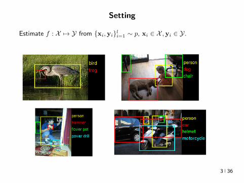
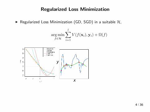
Regularized Loss Minimization
I Regularized Loss Minimization (GD SGD) in a suitable H
arg minfisinH
lsumi=1
V (f(xi)yi) + Ω(f)
I Understanding deep learning requires rethinking generalizationZhang et al 2017
4 36
Regularized Loss Minimization
I Regularized Loss Minimization (GD SGD) in a suitable H
arg minfisinH
lsumi=1
V (f(xi)yi) + Ω(f)
I Understanding deep learning requires rethinking generalizationZhang et al 2017
4 36
Optimization in Learning
I Optimal predictor
f = arg minf
E(xy)simpV (f(x)y)
I Approximation Error due to finite domain knowledge(Expressivity)
fH = arg minfisinH
E(xy)simpV (f(x)y)
I Estimation Error due to finite data (Generalization)
fH = arg minfisinH
lsumi=1
V (f(xi)yi) + Ω(f)
I Optimization Error finite computation (Optimization Landscape)
return f(i)H
Tractable but bad model or intractable but good model
5 36
Optimization in Learning
I Optimal predictor
f = arg minf
E(xy)simpV (f(x)y)
I Approximation Error due to finite domain knowledge(Expressivity)
fH = arg minfisinH
E(xy)simpV (f(x)y)
I Estimation Error due to finite data (Generalization)
fH = arg minfisinH
lsumi=1
V (f(xi)yi) + Ω(f)
I Optimization Error finite computation (Optimization Landscape)
return f(i)H
Tractable but bad model or intractable but good model 5 36
Nonlinearities Everywhere
Large l =rArr Big models H ldquorichrdquo non-parametricnonlinear
6 36
Nonlinearities Everywhere
Large l =rArr Big models H ldquorichrdquo non-parametricnonlinear
6 36
Nonlinearities Everywhere
Large l =rArr Big models H ldquorichrdquo non-parametricnonlinear
6 36
Choice of Nonlinear Hypothesis Space Kernels
x Ψ wTΨ(x) y
w
Ψ(x)
I eg Linear functions and Polynomials
I Infinite-dimensional nonlinear embeddings Fully non-parameteric
I Functional Analysis (Aronszajn Bergman (1950s)) Statistics (Parzen(1960s)) PDEs Numerical Analysis
I ML in 1990rsquos Nonlinear classification regression clustering time-seriesanalysis dynamical systems hypothesis testing causal modeling
I Convex Optimization
7 36
Choice of Nonlinear Hypothesis Space Kernels
x Ψ wTΨ(x) y
w
Ψ(x)
I eg Linear functions and Polynomials
I Infinite-dimensional nonlinear embeddings Fully non-parameteric
I Functional Analysis (Aronszajn Bergman (1950s)) Statistics (Parzen(1960s)) PDEs Numerical Analysis
I ML in 1990rsquos Nonlinear classification regression clustering time-seriesanalysis dynamical systems hypothesis testing causal modeling
I Convex Optimization
7 36
Choice of Nonlinear Hypothesis Space Kernels
x Ψ wTΨ(x) y
w
Ψ(x)
I eg Linear functions and Polynomials
I Infinite-dimensional nonlinear embeddings Fully non-parameteric
I Functional Analysis (Aronszajn Bergman (1950s)) Statistics (Parzen(1960s)) PDEs Numerical Analysis
I ML in 1990rsquos Nonlinear classification regression clustering time-seriesanalysis dynamical systems hypothesis testing causal modeling
I Convex Optimization
7 36
Choice of Nonlinear Hypothesis Space Kernels
x Ψ wTΨ(x) y
w
Ψ(x)
I eg Linear functions and Polynomials
I Infinite-dimensional nonlinear embeddings Fully non-parameteric
I Functional Analysis (Aronszajn Bergman (1950s)) Statistics (Parzen(1960s)) PDEs Numerical Analysis
I ML in 1990rsquos Nonlinear classification regression clustering time-seriesanalysis dynamical systems hypothesis testing causal modeling
I Convex Optimization
7 36
Choice of Nonlinear Hypothesis Space Kernels
x Ψ wTΨ(x) y
w
Ψ(x)
I eg Linear functions and Polynomials
I Infinite-dimensional nonlinear embeddings Fully non-parameteric
I Functional Analysis (Aronszajn Bergman (1950s)) Statistics (Parzen(1960s)) PDEs Numerical Analysis
I ML in 1990rsquos Nonlinear classification regression clustering time-seriesanalysis dynamical systems hypothesis testing causal modeling
I Convex Optimization
7 36
Choice of Nonlinear Hypothesis Space Deep Learning
x0 f1 f2 fL `
w1 w2 wL
z isin Rx1 x2 xLminus1 xL
I Compositions Raw data to higher abstractions (representation learning)
I Multilayer Perceptrons fl(xW) = σ(Wx) (sigmoids ReLU)I Turing (1950) In considering the functions of the mind or the brain we find certain operations which we can explain in
purely mechanical terms This we say does not correspond to the real mind it is a sort of skin which we must strip off if we are
to find the real mind Proceeding in this way do we ever come to the rdquorealrdquo mind or do we eventually come to the skin which
has nothing in it In the latter case the whole mind is mechanical
I Rosenblatt (1957) NYT 1958 New Navy Device Learns By Doing The Navy revealed the embryo of an electronic
computer today that it expects will be able to walk talk see write reproduce itself and be conscious of its existence Later
perceptrons will be able to recognize people and call out their names and instantly translate speech in one language to speech
and writing in another language it was predicted
I Perceptron (Minski and Pappert 1969) [Olarzan A Sociological Study 1996]I Backprop (1986) Reverse-mode differentiation (1960s-70s) CNNs (1980s 2012-)I Breadth-Width tradeoffsI Non-convex Optimization Domain-agnostic recipe
8 36
Choice of Nonlinear Hypothesis Space Deep Learning
x0 f1 f2 fL `
w1 w2 wL
z isin Rx1 x2 xLminus1 xL
I Compositions Raw data to higher abstractions (representation learning)I Multilayer Perceptrons fl(xW) = σ(Wx) (sigmoids ReLU)
I Turing (1950) In considering the functions of the mind or the brain we find certain operations which we can explain in
purely mechanical terms This we say does not correspond to the real mind it is a sort of skin which we must strip off if we are
to find the real mind Proceeding in this way do we ever come to the rdquorealrdquo mind or do we eventually come to the skin which
has nothing in it In the latter case the whole mind is mechanical
I Rosenblatt (1957) NYT 1958 New Navy Device Learns By Doing The Navy revealed the embryo of an electronic
computer today that it expects will be able to walk talk see write reproduce itself and be conscious of its existence Later
perceptrons will be able to recognize people and call out their names and instantly translate speech in one language to speech
and writing in another language it was predicted
I Perceptron (Minski and Pappert 1969) [Olarzan A Sociological Study 1996]I Backprop (1986) Reverse-mode differentiation (1960s-70s) CNNs (1980s 2012-)I Breadth-Width tradeoffsI Non-convex Optimization Domain-agnostic recipe
8 36
Choice of Nonlinear Hypothesis Space Deep Learning
x0 f1 f2 fL `
w1 w2 wL
z isin Rx1 x2 xLminus1 xL
I Compositions Raw data to higher abstractions (representation learning)I Multilayer Perceptrons fl(xW) = σ(Wx) (sigmoids ReLU)I Turing (1950) In considering the functions of the mind or the brain we find certain operations which we can explain in
purely mechanical terms This we say does not correspond to the real mind it is a sort of skin which we must strip off if we are
to find the real mind Proceeding in this way do we ever come to the rdquorealrdquo mind or do we eventually come to the skin which
has nothing in it In the latter case the whole mind is mechanical
I Rosenblatt (1957) NYT 1958 New Navy Device Learns By Doing The Navy revealed the embryo of an electronic
computer today that it expects will be able to walk talk see write reproduce itself and be conscious of its existence Later
perceptrons will be able to recognize people and call out their names and instantly translate speech in one language to speech
and writing in another language it was predicted
I Perceptron (Minski and Pappert 1969) [Olarzan A Sociological Study 1996]I Backprop (1986) Reverse-mode differentiation (1960s-70s) CNNs (1980s 2012-)I Breadth-Width tradeoffsI Non-convex Optimization Domain-agnostic recipe
8 36
Choice of Nonlinear Hypothesis Space Deep Learning
x0 f1 f2 fL `
w1 w2 wL
z isin Rx1 x2 xLminus1 xL
I Compositions Raw data to higher abstractions (representation learning)I Multilayer Perceptrons fl(xW) = σ(Wx) (sigmoids ReLU)I Turing (1950) In considering the functions of the mind or the brain we find certain operations which we can explain in
purely mechanical terms This we say does not correspond to the real mind it is a sort of skin which we must strip off if we are
to find the real mind Proceeding in this way do we ever come to the rdquorealrdquo mind or do we eventually come to the skin which
has nothing in it In the latter case the whole mind is mechanical
I Rosenblatt (1957) NYT 1958 New Navy Device Learns By Doing The Navy revealed the embryo of an electronic
computer today that it expects will be able to walk talk see write reproduce itself and be conscious of its existence Later
perceptrons will be able to recognize people and call out their names and instantly translate speech in one language to speech
and writing in another language it was predicted
I Perceptron (Minski and Pappert 1969) [Olarzan A Sociological Study 1996]I Backprop (1986) Reverse-mode differentiation (1960s-70s) CNNs (1980s 2012-)I Breadth-Width tradeoffsI Non-convex Optimization Domain-agnostic recipe
8 36
Choice of Nonlinear Hypothesis Space Deep Learning
x0 f1 f2 fL `
w1 w2 wL
z isin Rx1 x2 xLminus1 xL
I Compositions Raw data to higher abstractions (representation learning)I Multilayer Perceptrons fl(xW) = σ(Wx) (sigmoids ReLU)I Turing (1950) In considering the functions of the mind or the brain we find certain operations which we can explain in
purely mechanical terms This we say does not correspond to the real mind it is a sort of skin which we must strip off if we are
to find the real mind Proceeding in this way do we ever come to the rdquorealrdquo mind or do we eventually come to the skin which
has nothing in it In the latter case the whole mind is mechanical
I Rosenblatt (1957) NYT 1958 New Navy Device Learns By Doing The Navy revealed the embryo of an electronic
computer today that it expects will be able to walk talk see write reproduce itself and be conscious of its existence Later
perceptrons will be able to recognize people and call out their names and instantly translate speech in one language to speech
and writing in another language it was predicted
I Perceptron (Minski and Pappert 1969) [Olarzan A Sociological Study 1996]I Backprop (1986) Reverse-mode differentiation (1960s-70s) CNNs (1980s 2012-)
I Breadth-Width tradeoffsI Non-convex Optimization Domain-agnostic recipe
8 36
Choice of Nonlinear Hypothesis Space Deep Learning
x0 f1 f2 fL `
w1 w2 wL
z isin Rx1 x2 xLminus1 xL
I Compositions Raw data to higher abstractions (representation learning)I Multilayer Perceptrons fl(xW) = σ(Wx) (sigmoids ReLU)I Turing (1950) In considering the functions of the mind or the brain we find certain operations which we can explain in
purely mechanical terms This we say does not correspond to the real mind it is a sort of skin which we must strip off if we are
to find the real mind Proceeding in this way do we ever come to the rdquorealrdquo mind or do we eventually come to the skin which
has nothing in it In the latter case the whole mind is mechanical
I Rosenblatt (1957) NYT 1958 New Navy Device Learns By Doing The Navy revealed the embryo of an electronic
computer today that it expects will be able to walk talk see write reproduce itself and be conscious of its existence Later
perceptrons will be able to recognize people and call out their names and instantly translate speech in one language to speech
and writing in another language it was predicted
I Perceptron (Minski and Pappert 1969) [Olarzan A Sociological Study 1996]I Backprop (1986) Reverse-mode differentiation (1960s-70s) CNNs (1980s 2012-)I Breadth-Width tradeoffsI Non-convex Optimization Domain-agnostic recipe 8 36
Choice of Nonlinear Hypothesis Space Deep Learning
x0 f1 f2 fL `
w1 w2 wL
z isin Rx1 x2 xLminus1 xL
I Compositions Raw data to higher abstractions (representation learning)I Multilayer Perceptrons fl(xW) = σ(Wx) (sigmoids ReLU)I Turing (1950) In considering the functions of the mind or the brain we find certain operations which we can explain in
purely mechanical terms This we say does not correspond to the real mind it is a sort of skin which we must strip off if we are
to find the real mind Proceeding in this way do we ever come to the rdquorealrdquo mind or do we eventually come to the skin which
has nothing in it In the latter case the whole mind is mechanical
I Rosenblatt (1957) NYT 1958 New Navy Device Learns By Doing The Navy revealed the embryo of an electronic
computer today that it expects will be able to walk talk see write reproduce itself and be conscious of its existence Later
perceptrons will be able to recognize people and call out their names and instantly translate speech in one language to speech
and writing in another language it was predicted
I Perceptron (Minski and Pappert 1969) [Olarzan A Sociological Study 1996]I Backprop (1986) Reverse-mode differentiation (1960s-70s) CNNs (1980s 2012-)I Breadth-Width tradeoffsI Non-convex Optimization Domain-agnostic recipe 8 36
The Watershed Moment Imagenet 2012
I Many statistical and computational ingredientsndash Large datasets (ILSVRC since 2010)
ndash Large statistical capacity (12M images 60M params)ndash Distributed computationndash Depth Invariant feature learning (transferrable to other tasks)ndash Engineering Dropout ReLU
I Many astonishing results since then
9 36
The Watershed Moment Imagenet 2012
I Many statistical and computational ingredientsndash Large datasets (ILSVRC since 2010)ndash Large statistical capacity (12M images 60M params)
ndash Distributed computationndash Depth Invariant feature learning (transferrable to other tasks)ndash Engineering Dropout ReLU
I Many astonishing results since then
9 36
The Watershed Moment Imagenet 2012
I Many statistical and computational ingredientsndash Large datasets (ILSVRC since 2010)ndash Large statistical capacity (12M images 60M params)ndash Distributed computation
ndash Depth Invariant feature learning (transferrable to other tasks)ndash Engineering Dropout ReLU
I Many astonishing results since then
9 36
The Watershed Moment Imagenet 2012
I Many statistical and computational ingredientsndash Large datasets (ILSVRC since 2010)ndash Large statistical capacity (12M images 60M params)ndash Distributed computationndash Depth Invariant feature learning (transferrable to other tasks)
ndash Engineering Dropout ReLU I Many astonishing results since then
9 36
The Watershed Moment Imagenet 2012
I Many statistical and computational ingredientsndash Large datasets (ILSVRC since 2010)ndash Large statistical capacity (12M images 60M params)ndash Distributed computationndash Depth Invariant feature learning (transferrable to other tasks)ndash Engineering Dropout ReLU
I Many astonishing results since then
9 36
CNNs
10 36
Self-Driving Cars
Figure End-to-End Learning for Self-driving Cars Bojarski et al 2016
11 36

Regularized Loss Minimization
I Regularized Loss Minimization (GD SGD) in a suitable H
arg minfisinH
lsumi=1
V (f(xi)yi) + Ω(f)
I Understanding deep learning requires rethinking generalizationZhang et al 2017
4 36
Optimization in Learning
I Optimal predictor
f = arg minf
E(xy)simpV (f(x)y)
I Approximation Error due to finite domain knowledge(Expressivity)
fH = arg minfisinH
E(xy)simpV (f(x)y)
I Estimation Error due to finite data (Generalization)
fH = arg minfisinH
lsumi=1
V (f(xi)yi) + Ω(f)
I Optimization Error finite computation (Optimization Landscape)
return f(i)H
Tractable but bad model or intractable but good model
5 36
Optimization in Learning
I Optimal predictor
f = arg minf
E(xy)simpV (f(x)y)
I Approximation Error due to finite domain knowledge(Expressivity)
fH = arg minfisinH
E(xy)simpV (f(x)y)
I Estimation Error due to finite data (Generalization)
fH = arg minfisinH
lsumi=1
V (f(xi)yi) + Ω(f)
I Optimization Error finite computation (Optimization Landscape)
return f(i)H
Tractable but bad model or intractable but good model 5 36
Nonlinearities Everywhere
Large l =rArr Big models H ldquorichrdquo non-parametricnonlinear
6 36
Nonlinearities Everywhere
Large l =rArr Big models H ldquorichrdquo non-parametricnonlinear
6 36
Nonlinearities Everywhere
Large l =rArr Big models H ldquorichrdquo non-parametricnonlinear
6 36
Choice of Nonlinear Hypothesis Space Kernels
x Ψ wTΨ(x) y
w
Ψ(x)
I eg Linear functions and Polynomials
I Infinite-dimensional nonlinear embeddings Fully non-parameteric
I Functional Analysis (Aronszajn Bergman (1950s)) Statistics (Parzen(1960s)) PDEs Numerical Analysis
I ML in 1990rsquos Nonlinear classification regression clustering time-seriesanalysis dynamical systems hypothesis testing causal modeling
I Convex Optimization
7 36
Choice of Nonlinear Hypothesis Space Kernels
x Ψ wTΨ(x) y
w
Ψ(x)
I eg Linear functions and Polynomials
I Infinite-dimensional nonlinear embeddings Fully non-parameteric
I Functional Analysis (Aronszajn Bergman (1950s)) Statistics (Parzen(1960s)) PDEs Numerical Analysis
I ML in 1990rsquos Nonlinear classification regression clustering time-seriesanalysis dynamical systems hypothesis testing causal modeling
I Convex Optimization
7 36
Choice of Nonlinear Hypothesis Space Kernels
x Ψ wTΨ(x) y
w
Ψ(x)
I eg Linear functions and Polynomials
I Infinite-dimensional nonlinear embeddings Fully non-parameteric
I Functional Analysis (Aronszajn Bergman (1950s)) Statistics (Parzen(1960s)) PDEs Numerical Analysis
I ML in 1990rsquos Nonlinear classification regression clustering time-seriesanalysis dynamical systems hypothesis testing causal modeling
I Convex Optimization
7 36
Choice of Nonlinear Hypothesis Space Kernels
x Ψ wTΨ(x) y
w
Ψ(x)
I eg Linear functions and Polynomials
I Infinite-dimensional nonlinear embeddings Fully non-parameteric
I Functional Analysis (Aronszajn Bergman (1950s)) Statistics (Parzen(1960s)) PDEs Numerical Analysis
I ML in 1990rsquos Nonlinear classification regression clustering time-seriesanalysis dynamical systems hypothesis testing causal modeling
I Convex Optimization
7 36
Choice of Nonlinear Hypothesis Space Kernels
x Ψ wTΨ(x) y
w
Ψ(x)
I eg Linear functions and Polynomials
I Infinite-dimensional nonlinear embeddings Fully non-parameteric
I Functional Analysis (Aronszajn Bergman (1950s)) Statistics (Parzen(1960s)) PDEs Numerical Analysis
I ML in 1990rsquos Nonlinear classification regression clustering time-seriesanalysis dynamical systems hypothesis testing causal modeling
I Convex Optimization
7 36
Choice of Nonlinear Hypothesis Space Deep Learning
x0 f1 f2 fL `
w1 w2 wL
z isin Rx1 x2 xLminus1 xL
I Compositions Raw data to higher abstractions (representation learning)
I Multilayer Perceptrons fl(xW) = σ(Wx) (sigmoids ReLU)I Turing (1950) In considering the functions of the mind or the brain we find certain operations which we can explain in
purely mechanical terms This we say does not correspond to the real mind it is a sort of skin which we must strip off if we are
to find the real mind Proceeding in this way do we ever come to the rdquorealrdquo mind or do we eventually come to the skin which
has nothing in it In the latter case the whole mind is mechanical
I Rosenblatt (1957) NYT 1958 New Navy Device Learns By Doing The Navy revealed the embryo of an electronic
computer today that it expects will be able to walk talk see write reproduce itself and be conscious of its existence Later
perceptrons will be able to recognize people and call out their names and instantly translate speech in one language to speech
and writing in another language it was predicted
I Perceptron (Minski and Pappert 1969) [Olarzan A Sociological Study 1996]I Backprop (1986) Reverse-mode differentiation (1960s-70s) CNNs (1980s 2012-)I Breadth-Width tradeoffsI Non-convex Optimization Domain-agnostic recipe
8 36
Choice of Nonlinear Hypothesis Space Deep Learning
x0 f1 f2 fL `
w1 w2 wL
z isin Rx1 x2 xLminus1 xL
I Compositions Raw data to higher abstractions (representation learning)I Multilayer Perceptrons fl(xW) = σ(Wx) (sigmoids ReLU)
I Turing (1950) In considering the functions of the mind or the brain we find certain operations which we can explain in
purely mechanical terms This we say does not correspond to the real mind it is a sort of skin which we must strip off if we are
to find the real mind Proceeding in this way do we ever come to the rdquorealrdquo mind or do we eventually come to the skin which
has nothing in it In the latter case the whole mind is mechanical
I Rosenblatt (1957) NYT 1958 New Navy Device Learns By Doing The Navy revealed the embryo of an electronic
computer today that it expects will be able to walk talk see write reproduce itself and be conscious of its existence Later
perceptrons will be able to recognize people and call out their names and instantly translate speech in one language to speech
and writing in another language it was predicted
I Perceptron (Minski and Pappert 1969) [Olarzan A Sociological Study 1996]I Backprop (1986) Reverse-mode differentiation (1960s-70s) CNNs (1980s 2012-)I Breadth-Width tradeoffsI Non-convex Optimization Domain-agnostic recipe
8 36
Choice of Nonlinear Hypothesis Space Deep Learning
x0 f1 f2 fL `
w1 w2 wL
z isin Rx1 x2 xLminus1 xL
I Compositions Raw data to higher abstractions (representation learning)I Multilayer Perceptrons fl(xW) = σ(Wx) (sigmoids ReLU)I Turing (1950) In considering the functions of the mind or the brain we find certain operations which we can explain in
purely mechanical terms This we say does not correspond to the real mind it is a sort of skin which we must strip off if we are
to find the real mind Proceeding in this way do we ever come to the rdquorealrdquo mind or do we eventually come to the skin which
has nothing in it In the latter case the whole mind is mechanical
I Rosenblatt (1957) NYT 1958 New Navy Device Learns By Doing The Navy revealed the embryo of an electronic
computer today that it expects will be able to walk talk see write reproduce itself and be conscious of its existence Later
perceptrons will be able to recognize people and call out their names and instantly translate speech in one language to speech
and writing in another language it was predicted
I Perceptron (Minski and Pappert 1969) [Olarzan A Sociological Study 1996]I Backprop (1986) Reverse-mode differentiation (1960s-70s) CNNs (1980s 2012-)I Breadth-Width tradeoffsI Non-convex Optimization Domain-agnostic recipe
8 36
Choice of Nonlinear Hypothesis Space Deep Learning
x0 f1 f2 fL `
w1 w2 wL
z isin Rx1 x2 xLminus1 xL
I Compositions Raw data to higher abstractions (representation learning)I Multilayer Perceptrons fl(xW) = σ(Wx) (sigmoids ReLU)I Turing (1950) In considering the functions of the mind or the brain we find certain operations which we can explain in
purely mechanical terms This we say does not correspond to the real mind it is a sort of skin which we must strip off if we are
to find the real mind Proceeding in this way do we ever come to the rdquorealrdquo mind or do we eventually come to the skin which
has nothing in it In the latter case the whole mind is mechanical
I Rosenblatt (1957) NYT 1958 New Navy Device Learns By Doing The Navy revealed the embryo of an electronic
computer today that it expects will be able to walk talk see write reproduce itself and be conscious of its existence Later
perceptrons will be able to recognize people and call out their names and instantly translate speech in one language to speech
and writing in another language it was predicted
I Perceptron (Minski and Pappert 1969) [Olarzan A Sociological Study 1996]I Backprop (1986) Reverse-mode differentiation (1960s-70s) CNNs (1980s 2012-)I Breadth-Width tradeoffsI Non-convex Optimization Domain-agnostic recipe
8 36
Choice of Nonlinear Hypothesis Space Deep Learning
x0 f1 f2 fL `
w1 w2 wL
z isin Rx1 x2 xLminus1 xL
I Compositions Raw data to higher abstractions (representation learning)I Multilayer Perceptrons fl(xW) = σ(Wx) (sigmoids ReLU)I Turing (1950) In considering the functions of the mind or the brain we find certain operations which we can explain in
purely mechanical terms This we say does not correspond to the real mind it is a sort of skin which we must strip off if we are
to find the real mind Proceeding in this way do we ever come to the rdquorealrdquo mind or do we eventually come to the skin which
has nothing in it In the latter case the whole mind is mechanical
I Rosenblatt (1957) NYT 1958 New Navy Device Learns By Doing The Navy revealed the embryo of an electronic
computer today that it expects will be able to walk talk see write reproduce itself and be conscious of its existence Later
perceptrons will be able to recognize people and call out their names and instantly translate speech in one language to speech
and writing in another language it was predicted
I Perceptron (Minski and Pappert 1969) [Olarzan A Sociological Study 1996]I Backprop (1986) Reverse-mode differentiation (1960s-70s) CNNs (1980s 2012-)
I Breadth-Width tradeoffsI Non-convex Optimization Domain-agnostic recipe
8 36
Choice of Nonlinear Hypothesis Space Deep Learning
x0 f1 f2 fL `
w1 w2 wL
z isin Rx1 x2 xLminus1 xL
I Compositions Raw data to higher abstractions (representation learning)I Multilayer Perceptrons fl(xW) = σ(Wx) (sigmoids ReLU)I Turing (1950) In considering the functions of the mind or the brain we find certain operations which we can explain in
purely mechanical terms This we say does not correspond to the real mind it is a sort of skin which we must strip off if we are
to find the real mind Proceeding in this way do we ever come to the rdquorealrdquo mind or do we eventually come to the skin which
has nothing in it In the latter case the whole mind is mechanical
I Rosenblatt (1957) NYT 1958 New Navy Device Learns By Doing The Navy revealed the embryo of an electronic
computer today that it expects will be able to walk talk see write reproduce itself and be conscious of its existence Later
perceptrons will be able to recognize people and call out their names and instantly translate speech in one language to speech
and writing in another language it was predicted
I Perceptron (Minski and Pappert 1969) [Olarzan A Sociological Study 1996]I Backprop (1986) Reverse-mode differentiation (1960s-70s) CNNs (1980s 2012-)I Breadth-Width tradeoffsI Non-convex Optimization Domain-agnostic recipe 8 36
Choice of Nonlinear Hypothesis Space Deep Learning
x0 f1 f2 fL `
w1 w2 wL
z isin Rx1 x2 xLminus1 xL
I Compositions Raw data to higher abstractions (representation learning)I Multilayer Perceptrons fl(xW) = σ(Wx) (sigmoids ReLU)I Turing (1950) In considering the functions of the mind or the brain we find certain operations which we can explain in
purely mechanical terms This we say does not correspond to the real mind it is a sort of skin which we must strip off if we are
to find the real mind Proceeding in this way do we ever come to the rdquorealrdquo mind or do we eventually come to the skin which
has nothing in it In the latter case the whole mind is mechanical
I Rosenblatt (1957) NYT 1958 New Navy Device Learns By Doing The Navy revealed the embryo of an electronic
computer today that it expects will be able to walk talk see write reproduce itself and be conscious of its existence Later
perceptrons will be able to recognize people and call out their names and instantly translate speech in one language to speech
and writing in another language it was predicted
I Perceptron (Minski and Pappert 1969) [Olarzan A Sociological Study 1996]I Backprop (1986) Reverse-mode differentiation (1960s-70s) CNNs (1980s 2012-)I Breadth-Width tradeoffsI Non-convex Optimization Domain-agnostic recipe 8 36
The Watershed Moment Imagenet 2012
I Many statistical and computational ingredientsndash Large datasets (ILSVRC since 2010)
ndash Large statistical capacity (12M images 60M params)ndash Distributed computationndash Depth Invariant feature learning (transferrable to other tasks)ndash Engineering Dropout ReLU
I Many astonishing results since then
9 36
The Watershed Moment Imagenet 2012
I Many statistical and computational ingredientsndash Large datasets (ILSVRC since 2010)ndash Large statistical capacity (12M images 60M params)
ndash Distributed computationndash Depth Invariant feature learning (transferrable to other tasks)ndash Engineering Dropout ReLU
I Many astonishing results since then
9 36
The Watershed Moment Imagenet 2012
I Many statistical and computational ingredientsndash Large datasets (ILSVRC since 2010)ndash Large statistical capacity (12M images 60M params)ndash Distributed computation
ndash Depth Invariant feature learning (transferrable to other tasks)ndash Engineering Dropout ReLU
I Many astonishing results since then
9 36
The Watershed Moment Imagenet 2012
I Many statistical and computational ingredientsndash Large datasets (ILSVRC since 2010)ndash Large statistical capacity (12M images 60M params)ndash Distributed computationndash Depth Invariant feature learning (transferrable to other tasks)
ndash Engineering Dropout ReLU I Many astonishing results since then
9 36
The Watershed Moment Imagenet 2012
I Many statistical and computational ingredientsndash Large datasets (ILSVRC since 2010)ndash Large statistical capacity (12M images 60M params)ndash Distributed computationndash Depth Invariant feature learning (transferrable to other tasks)ndash Engineering Dropout ReLU
I Many astonishing results since then
9 36
CNNs
10 36
Self-Driving Cars
Figure End-to-End Learning for Self-driving Cars Bojarski et al 2016
11 36

Optimization in Learning
I Optimal predictor
f = arg minf
E(xy)simpV (f(x)y)
I Approximation Error due to finite domain knowledge(Expressivity)
fH = arg minfisinH
E(xy)simpV (f(x)y)
I Estimation Error due to finite data (Generalization)
fH = arg minfisinH
lsumi=1
V (f(xi)yi) + Ω(f)
I Optimization Error finite computation (Optimization Landscape)
return f(i)H
Tractable but bad model or intractable but good model
5 36
Optimization in Learning
I Optimal predictor
f = arg minf
E(xy)simpV (f(x)y)
I Approximation Error due to finite domain knowledge(Expressivity)
fH = arg minfisinH
E(xy)simpV (f(x)y)
I Estimation Error due to finite data (Generalization)
fH = arg minfisinH
lsumi=1
V (f(xi)yi) + Ω(f)
I Optimization Error finite computation (Optimization Landscape)
return f(i)H
Tractable but bad model or intractable but good model 5 36
Nonlinearities Everywhere
Large l =rArr Big models H ldquorichrdquo non-parametricnonlinear
6 36
Nonlinearities Everywhere
Large l =rArr Big models H ldquorichrdquo non-parametricnonlinear
6 36
Nonlinearities Everywhere
Large l =rArr Big models H ldquorichrdquo non-parametricnonlinear
6 36
Choice of Nonlinear Hypothesis Space Kernels
x Ψ wTΨ(x) y
w
Ψ(x)
I eg Linear functions and Polynomials
I Infinite-dimensional nonlinear embeddings Fully non-parameteric
I Functional Analysis (Aronszajn Bergman (1950s)) Statistics (Parzen(1960s)) PDEs Numerical Analysis
I ML in 1990rsquos Nonlinear classification regression clustering time-seriesanalysis dynamical systems hypothesis testing causal modeling
I Convex Optimization
7 36
Choice of Nonlinear Hypothesis Space Kernels
x Ψ wTΨ(x) y
w
Ψ(x)
I eg Linear functions and Polynomials
I Infinite-dimensional nonlinear embeddings Fully non-parameteric
I Functional Analysis (Aronszajn Bergman (1950s)) Statistics (Parzen(1960s)) PDEs Numerical Analysis
I ML in 1990rsquos Nonlinear classification regression clustering time-seriesanalysis dynamical systems hypothesis testing causal modeling
I Convex Optimization
7 36
Choice of Nonlinear Hypothesis Space Kernels
x Ψ wTΨ(x) y
w
Ψ(x)
I eg Linear functions and Polynomials
I Infinite-dimensional nonlinear embeddings Fully non-parameteric
I Functional Analysis (Aronszajn Bergman (1950s)) Statistics (Parzen(1960s)) PDEs Numerical Analysis
I ML in 1990rsquos Nonlinear classification regression clustering time-seriesanalysis dynamical systems hypothesis testing causal modeling
I Convex Optimization
7 36
Choice of Nonlinear Hypothesis Space Kernels
x Ψ wTΨ(x) y
w
Ψ(x)
I eg Linear functions and Polynomials
I Infinite-dimensional nonlinear embeddings Fully non-parameteric
I Functional Analysis (Aronszajn Bergman (1950s)) Statistics (Parzen(1960s)) PDEs Numerical Analysis
I ML in 1990rsquos Nonlinear classification regression clustering time-seriesanalysis dynamical systems hypothesis testing causal modeling
I Convex Optimization
7 36
Choice of Nonlinear Hypothesis Space Kernels
x Ψ wTΨ(x) y
w
Ψ(x)
I eg Linear functions and Polynomials
I Infinite-dimensional nonlinear embeddings Fully non-parameteric
I Functional Analysis (Aronszajn Bergman (1950s)) Statistics (Parzen(1960s)) PDEs Numerical Analysis
I ML in 1990rsquos Nonlinear classification regression clustering time-seriesanalysis dynamical systems hypothesis testing causal modeling
I Convex Optimization
7 36
Choice of Nonlinear Hypothesis Space Deep Learning
x0 f1 f2 fL `
w1 w2 wL
z isin Rx1 x2 xLminus1 xL
I Compositions Raw data to higher abstractions (representation learning)
I Multilayer Perceptrons fl(xW) = σ(Wx) (sigmoids ReLU)I Turing (1950) In considering the functions of the mind or the brain we find certain operations which we can explain in
purely mechanical terms This we say does not correspond to the real mind it is a sort of skin which we must strip off if we are
to find the real mind Proceeding in this way do we ever come to the rdquorealrdquo mind or do we eventually come to the skin which
has nothing in it In the latter case the whole mind is mechanical
I Rosenblatt (1957) NYT 1958 New Navy Device Learns By Doing The Navy revealed the embryo of an electronic
computer today that it expects will be able to walk talk see write reproduce itself and be conscious of its existence Later
perceptrons will be able to recognize people and call out their names and instantly translate speech in one language to speech
and writing in another language it was predicted
I Perceptron (Minski and Pappert 1969) [Olarzan A Sociological Study 1996]I Backprop (1986) Reverse-mode differentiation (1960s-70s) CNNs (1980s 2012-)I Breadth-Width tradeoffsI Non-convex Optimization Domain-agnostic recipe
8 36
Choice of Nonlinear Hypothesis Space Deep Learning
x0 f1 f2 fL `
w1 w2 wL
z isin Rx1 x2 xLminus1 xL
I Compositions Raw data to higher abstractions (representation learning)I Multilayer Perceptrons fl(xW) = σ(Wx) (sigmoids ReLU)
I Turing (1950) In considering the functions of the mind or the brain we find certain operations which we can explain in
purely mechanical terms This we say does not correspond to the real mind it is a sort of skin which we must strip off if we are
to find the real mind Proceeding in this way do we ever come to the rdquorealrdquo mind or do we eventually come to the skin which
has nothing in it In the latter case the whole mind is mechanical
I Rosenblatt (1957) NYT 1958 New Navy Device Learns By Doing The Navy revealed the embryo of an electronic
computer today that it expects will be able to walk talk see write reproduce itself and be conscious of its existence Later
perceptrons will be able to recognize people and call out their names and instantly translate speech in one language to speech
and writing in another language it was predicted
I Perceptron (Minski and Pappert 1969) [Olarzan A Sociological Study 1996]I Backprop (1986) Reverse-mode differentiation (1960s-70s) CNNs (1980s 2012-)I Breadth-Width tradeoffsI Non-convex Optimization Domain-agnostic recipe
8 36
Choice of Nonlinear Hypothesis Space Deep Learning
x0 f1 f2 fL `
w1 w2 wL
z isin Rx1 x2 xLminus1 xL
I Compositions Raw data to higher abstractions (representation learning)I Multilayer Perceptrons fl(xW) = σ(Wx) (sigmoids ReLU)I Turing (1950) In considering the functions of the mind or the brain we find certain operations which we can explain in
purely mechanical terms This we say does not correspond to the real mind it is a sort of skin which we must strip off if we are
to find the real mind Proceeding in this way do we ever come to the rdquorealrdquo mind or do we eventually come to the skin which
has nothing in it In the latter case the whole mind is mechanical
I Rosenblatt (1957) NYT 1958 New Navy Device Learns By Doing The Navy revealed the embryo of an electronic
computer today that it expects will be able to walk talk see write reproduce itself and be conscious of its existence Later
perceptrons will be able to recognize people and call out their names and instantly translate speech in one language to speech
and writing in another language it was predicted
I Perceptron (Minski and Pappert 1969) [Olarzan A Sociological Study 1996]I Backprop (1986) Reverse-mode differentiation (1960s-70s) CNNs (1980s 2012-)I Breadth-Width tradeoffsI Non-convex Optimization Domain-agnostic recipe
8 36
Choice of Nonlinear Hypothesis Space Deep Learning
x0 f1 f2 fL `
w1 w2 wL
z isin Rx1 x2 xLminus1 xL
I Compositions Raw data to higher abstractions (representation learning)I Multilayer Perceptrons fl(xW) = σ(Wx) (sigmoids ReLU)I Turing (1950) In considering the functions of the mind or the brain we find certain operations which we can explain in
purely mechanical terms This we say does not correspond to the real mind it is a sort of skin which we must strip off if we are
to find the real mind Proceeding in this way do we ever come to the rdquorealrdquo mind or do we eventually come to the skin which
has nothing in it In the latter case the whole mind is mechanical
I Rosenblatt (1957) NYT 1958 New Navy Device Learns By Doing The Navy revealed the embryo of an electronic
computer today that it expects will be able to walk talk see write reproduce itself and be conscious of its existence Later
perceptrons will be able to recognize people and call out their names and instantly translate speech in one language to speech
and writing in another language it was predicted
I Perceptron (Minski and Pappert 1969) [Olarzan A Sociological Study 1996]I Backprop (1986) Reverse-mode differentiation (1960s-70s) CNNs (1980s 2012-)I Breadth-Width tradeoffsI Non-convex Optimization Domain-agnostic recipe
8 36
Choice of Nonlinear Hypothesis Space Deep Learning
x0 f1 f2 fL `
w1 w2 wL
z isin Rx1 x2 xLminus1 xL
I Compositions Raw data to higher abstractions (representation learning)I Multilayer Perceptrons fl(xW) = σ(Wx) (sigmoids ReLU)I Turing (1950) In considering the functions of the mind or the brain we find certain operations which we can explain in
purely mechanical terms This we say does not correspond to the real mind it is a sort of skin which we must strip off if we are
to find the real mind Proceeding in this way do we ever come to the rdquorealrdquo mind or do we eventually come to the skin which
has nothing in it In the latter case the whole mind is mechanical
I Rosenblatt (1957) NYT 1958 New Navy Device Learns By Doing The Navy revealed the embryo of an electronic
computer today that it expects will be able to walk talk see write reproduce itself and be conscious of its existence Later
perceptrons will be able to recognize people and call out their names and instantly translate speech in one language to speech
and writing in another language it was predicted
I Perceptron (Minski and Pappert 1969) [Olarzan A Sociological Study 1996]I Backprop (1986) Reverse-mode differentiation (1960s-70s) CNNs (1980s 2012-)
I Breadth-Width tradeoffsI Non-convex Optimization Domain-agnostic recipe
8 36
Choice of Nonlinear Hypothesis Space Deep Learning
x0 f1 f2 fL `
w1 w2 wL
z isin Rx1 x2 xLminus1 xL
I Compositions Raw data to higher abstractions (representation learning)I Multilayer Perceptrons fl(xW) = σ(Wx) (sigmoids ReLU)I Turing (1950) In considering the functions of the mind or the brain we find certain operations which we can explain in
purely mechanical terms This we say does not correspond to the real mind it is a sort of skin which we must strip off if we are
to find the real mind Proceeding in this way do we ever come to the rdquorealrdquo mind or do we eventually come to the skin which
has nothing in it In the latter case the whole mind is mechanical
I Rosenblatt (1957) NYT 1958 New Navy Device Learns By Doing The Navy revealed the embryo of an electronic
computer today that it expects will be able to walk talk see write reproduce itself and be conscious of its existence Later
perceptrons will be able to recognize people and call out their names and instantly translate speech in one language to speech
and writing in another language it was predicted
I Perceptron (Minski and Pappert 1969) [Olarzan A Sociological Study 1996]I Backprop (1986) Reverse-mode differentiation (1960s-70s) CNNs (1980s 2012-)I Breadth-Width tradeoffsI Non-convex Optimization Domain-agnostic recipe 8 36
Choice of Nonlinear Hypothesis Space Deep Learning
x0 f1 f2 fL `
w1 w2 wL
z isin Rx1 x2 xLminus1 xL
I Compositions Raw data to higher abstractions (representation learning)I Multilayer Perceptrons fl(xW) = σ(Wx) (sigmoids ReLU)I Turing (1950) In considering the functions of the mind or the brain we find certain operations which we can explain in
purely mechanical terms This we say does not correspond to the real mind it is a sort of skin which we must strip off if we are
to find the real mind Proceeding in this way do we ever come to the rdquorealrdquo mind or do we eventually come to the skin which
has nothing in it In the latter case the whole mind is mechanical
I Rosenblatt (1957) NYT 1958 New Navy Device Learns By Doing The Navy revealed the embryo of an electronic
computer today that it expects will be able to walk talk see write reproduce itself and be conscious of its existence Later
perceptrons will be able to recognize people and call out their names and instantly translate speech in one language to speech
and writing in another language it was predicted
I Perceptron (Minski and Pappert 1969) [Olarzan A Sociological Study 1996]I Backprop (1986) Reverse-mode differentiation (1960s-70s) CNNs (1980s 2012-)I Breadth-Width tradeoffsI Non-convex Optimization Domain-agnostic recipe 8 36
The Watershed Moment Imagenet 2012
I Many statistical and computational ingredientsndash Large datasets (ILSVRC since 2010)
ndash Large statistical capacity (12M images 60M params)ndash Distributed computationndash Depth Invariant feature learning (transferrable to other tasks)ndash Engineering Dropout ReLU
I Many astonishing results since then
9 36
The Watershed Moment Imagenet 2012
I Many statistical and computational ingredientsndash Large datasets (ILSVRC since 2010)ndash Large statistical capacity (12M images 60M params)
ndash Distributed computationndash Depth Invariant feature learning (transferrable to other tasks)ndash Engineering Dropout ReLU
I Many astonishing results since then
9 36
The Watershed Moment Imagenet 2012
I Many statistical and computational ingredientsndash Large datasets (ILSVRC since 2010)ndash Large statistical capacity (12M images 60M params)ndash Distributed computation
ndash Depth Invariant feature learning (transferrable to other tasks)ndash Engineering Dropout ReLU
I Many astonishing results since then
9 36
The Watershed Moment Imagenet 2012
I Many statistical and computational ingredientsndash Large datasets (ILSVRC since 2010)ndash Large statistical capacity (12M images 60M params)ndash Distributed computationndash Depth Invariant feature learning (transferrable to other tasks)
ndash Engineering Dropout ReLU I Many astonishing results since then
9 36
The Watershed Moment Imagenet 2012
I Many statistical and computational ingredientsndash Large datasets (ILSVRC since 2010)ndash Large statistical capacity (12M images 60M params)ndash Distributed computationndash Depth Invariant feature learning (transferrable to other tasks)ndash Engineering Dropout ReLU
I Many astonishing results since then
9 36
CNNs
10 36
Self-Driving Cars
Figure End-to-End Learning for Self-driving Cars Bojarski et al 2016
11 36

Optimization in Learning
I Optimal predictor
f = arg minf
E(xy)simpV (f(x)y)
I Approximation Error due to finite domain knowledge(Expressivity)
fH = arg minfisinH
E(xy)simpV (f(x)y)
I Estimation Error due to finite data (Generalization)
fH = arg minfisinH
lsumi=1
V (f(xi)yi) + Ω(f)
I Optimization Error finite computation (Optimization Landscape)
return f(i)H
Tractable but bad model or intractable but good model
5 36
Optimization in Learning
I Optimal predictor
f = arg minf
E(xy)simpV (f(x)y)
I Approximation Error due to finite domain knowledge(Expressivity)
fH = arg minfisinH
E(xy)simpV (f(x)y)
I Estimation Error due to finite data (Generalization)
fH = arg minfisinH
lsumi=1
V (f(xi)yi) + Ω(f)
I Optimization Error finite computation (Optimization Landscape)
return f(i)H
Tractable but bad model or intractable but good model
5 36
Optimization in Learning
I Optimal predictor
f = arg minf
E(xy)simpV (f(x)y)
I Approximation Error due to finite domain knowledge(Expressivity)
fH = arg minfisinH
E(xy)simpV (f(x)y)
I Estimation Error due to finite data (Generalization)
fH = arg minfisinH
lsumi=1
V (f(xi)yi) + Ω(f)
I Optimization Error finite computation (Optimization Landscape)
return f(i)H
Tractable but bad model or intractable but good model
5 36
Optimization in Learning
I Optimal predictor
f = arg minf
E(xy)simpV (f(x)y)
I Approximation Error due to finite domain knowledge(Expressivity)
fH = arg minfisinH
E(xy)simpV (f(x)y)
I Estimation Error due to finite data (Generalization)
fH = arg minfisinH
lsumi=1
V (f(xi)yi) + Ω(f)
I Optimization Error finite computation (Optimization Landscape)
return f(i)H
Tractable but bad model or intractable but good model 5 36
Nonlinearities Everywhere
Large l =rArr Big models H ldquorichrdquo non-parametricnonlinear
6 36
Nonlinearities Everywhere
Large l =rArr Big models H ldquorichrdquo non-parametricnonlinear
6 36
Nonlinearities Everywhere
Large l =rArr Big models H ldquorichrdquo non-parametricnonlinear
6 36
Choice of Nonlinear Hypothesis Space Kernels
x Ψ wTΨ(x) y
w
Ψ(x)
I eg Linear functions and Polynomials
I Infinite-dimensional nonlinear embeddings Fully non-parameteric
I Functional Analysis (Aronszajn Bergman (1950s)) Statistics (Parzen(1960s)) PDEs Numerical Analysis
I ML in 1990rsquos Nonlinear classification regression clustering time-seriesanalysis dynamical systems hypothesis testing causal modeling
I Convex Optimization
7 36
Choice of Nonlinear Hypothesis Space Kernels
x Ψ wTΨ(x) y
w
Ψ(x)
I eg Linear functions and Polynomials
I Infinite-dimensional nonlinear embeddings Fully non-parameteric
I Functional Analysis (Aronszajn Bergman (1950s)) Statistics (Parzen(1960s)) PDEs Numerical Analysis
I ML in 1990rsquos Nonlinear classification regression clustering time-seriesanalysis dynamical systems hypothesis testing causal modeling
I Convex Optimization
7 36
Choice of Nonlinear Hypothesis Space Kernels
x Ψ wTΨ(x) y
w
Ψ(x)
I eg Linear functions and Polynomials
I Infinite-dimensional nonlinear embeddings Fully non-parameteric
I Functional Analysis (Aronszajn Bergman (1950s)) Statistics (Parzen(1960s)) PDEs Numerical Analysis
I ML in 1990rsquos Nonlinear classification regression clustering time-seriesanalysis dynamical systems hypothesis testing causal modeling
I Convex Optimization
7 36
Choice of Nonlinear Hypothesis Space Kernels
x Ψ wTΨ(x) y
w
Ψ(x)
I eg Linear functions and Polynomials
I Infinite-dimensional nonlinear embeddings Fully non-parameteric
I Functional Analysis (Aronszajn Bergman (1950s)) Statistics (Parzen(1960s)) PDEs Numerical Analysis
I ML in 1990rsquos Nonlinear classification regression clustering time-seriesanalysis dynamical systems hypothesis testing causal modeling
I Convex Optimization
7 36
Choice of Nonlinear Hypothesis Space Kernels
x Ψ wTΨ(x) y
w
Ψ(x)
I eg Linear functions and Polynomials
I Infinite-dimensional nonlinear embeddings Fully non-parameteric
I Functional Analysis (Aronszajn Bergman (1950s)) Statistics (Parzen(1960s)) PDEs Numerical Analysis
I ML in 1990rsquos Nonlinear classification regression clustering time-seriesanalysis dynamical systems hypothesis testing causal modeling
I Convex Optimization
7 36
Choice of Nonlinear Hypothesis Space Deep Learning
x0 f1 f2 fL `
w1 w2 wL
z isin Rx1 x2 xLminus1 xL
I Compositions Raw data to higher abstractions (representation learning)
I Multilayer Perceptrons fl(xW) = σ(Wx) (sigmoids ReLU)I Turing (1950) In considering the functions of the mind or the brain we find certain operations which we can explain in
purely mechanical terms This we say does not correspond to the real mind it is a sort of skin which we must strip off if we are
to find the real mind Proceeding in this way do we ever come to the rdquorealrdquo mind or do we eventually come to the skin which
has nothing in it In the latter case the whole mind is mechanical
I Rosenblatt (1957) NYT 1958 New Navy Device Learns By Doing The Navy revealed the embryo of an electronic
computer today that it expects will be able to walk talk see write reproduce itself and be conscious of its existence Later
perceptrons will be able to recognize people and call out their names and instantly translate speech in one language to speech
and writing in another language it was predicted
I Perceptron (Minski and Pappert 1969) [Olarzan A Sociological Study 1996]I Backprop (1986) Reverse-mode differentiation (1960s-70s) CNNs (1980s 2012-)I Breadth-Width tradeoffsI Non-convex Optimization Domain-agnostic recipe
8 36
Choice of Nonlinear Hypothesis Space Deep Learning
x0 f1 f2 fL `
w1 w2 wL
z isin Rx1 x2 xLminus1 xL
I Compositions Raw data to higher abstractions (representation learning)I Multilayer Perceptrons fl(xW) = σ(Wx) (sigmoids ReLU)
I Turing (1950) In considering the functions of the mind or the brain we find certain operations which we can explain in
purely mechanical terms This we say does not correspond to the real mind it is a sort of skin which we must strip off if we are
to find the real mind Proceeding in this way do we ever come to the rdquorealrdquo mind or do we eventually come to the skin which
has nothing in it In the latter case the whole mind is mechanical
I Rosenblatt (1957) NYT 1958 New Navy Device Learns By Doing The Navy revealed the embryo of an electronic
computer today that it expects will be able to walk talk see write reproduce itself and be conscious of its existence Later
perceptrons will be able to recognize people and call out their names and instantly translate speech in one language to speech
and writing in another language it was predicted
I Perceptron (Minski and Pappert 1969) [Olarzan A Sociological Study 1996]I Backprop (1986) Reverse-mode differentiation (1960s-70s) CNNs (1980s 2012-)I Breadth-Width tradeoffsI Non-convex Optimization Domain-agnostic recipe
8 36
Choice of Nonlinear Hypothesis Space Deep Learning
x0 f1 f2 fL `
w1 w2 wL
z isin Rx1 x2 xLminus1 xL
I Compositions Raw data to higher abstractions (representation learning)I Multilayer Perceptrons fl(xW) = σ(Wx) (sigmoids ReLU)I Turing (1950) In considering the functions of the mind or the brain we find certain operations which we can explain in
purely mechanical terms This we say does not correspond to the real mind it is a sort of skin which we must strip off if we are
to find the real mind Proceeding in this way do we ever come to the rdquorealrdquo mind or do we eventually come to the skin which
has nothing in it In the latter case the whole mind is mechanical
I Rosenblatt (1957) NYT 1958 New Navy Device Learns By Doing The Navy revealed the embryo of an electronic
computer today that it expects will be able to walk talk see write reproduce itself and be conscious of its existence Later
perceptrons will be able to recognize people and call out their names and instantly translate speech in one language to speech
and writing in another language it was predicted
I Perceptron (Minski and Pappert 1969) [Olarzan A Sociological Study 1996]I Backprop (1986) Reverse-mode differentiation (1960s-70s) CNNs (1980s 2012-)I Breadth-Width tradeoffsI Non-convex Optimization Domain-agnostic recipe
8 36
Choice of Nonlinear Hypothesis Space Deep Learning
x0 f1 f2 fL `
w1 w2 wL
z isin Rx1 x2 xLminus1 xL
I Compositions Raw data to higher abstractions (representation learning)I Multilayer Perceptrons fl(xW) = σ(Wx) (sigmoids ReLU)I Turing (1950) In considering the functions of the mind or the brain we find certain operations which we can explain in
purely mechanical terms This we say does not correspond to the real mind it is a sort of skin which we must strip off if we are
to find the real mind Proceeding in this way do we ever come to the rdquorealrdquo mind or do we eventually come to the skin which
has nothing in it In the latter case the whole mind is mechanical
I Rosenblatt (1957) NYT 1958 New Navy Device Learns By Doing The Navy revealed the embryo of an electronic
computer today that it expects will be able to walk talk see write reproduce itself and be conscious of its existence Later
perceptrons will be able to recognize people and call out their names and instantly translate speech in one language to speech
and writing in another language it was predicted
I Perceptron (Minski and Pappert 1969) [Olarzan A Sociological Study 1996]I Backprop (1986) Reverse-mode differentiation (1960s-70s) CNNs (1980s 2012-)I Breadth-Width tradeoffsI Non-convex Optimization Domain-agnostic recipe
8 36
Choice of Nonlinear Hypothesis Space Deep Learning
x0 f1 f2 fL `
w1 w2 wL
z isin Rx1 x2 xLminus1 xL
I Compositions Raw data to higher abstractions (representation learning)I Multilayer Perceptrons fl(xW) = σ(Wx) (sigmoids ReLU)I Turing (1950) In considering the functions of the mind or the brain we find certain operations which we can explain in
purely mechanical terms This we say does not correspond to the real mind it is a sort of skin which we must strip off if we are
to find the real mind Proceeding in this way do we ever come to the rdquorealrdquo mind or do we eventually come to the skin which
has nothing in it In the latter case the whole mind is mechanical
I Rosenblatt (1957) NYT 1958 New Navy Device Learns By Doing The Navy revealed the embryo of an electronic
computer today that it expects will be able to walk talk see write reproduce itself and be conscious of its existence Later
perceptrons will be able to recognize people and call out their names and instantly translate speech in one language to speech
and writing in another language it was predicted
I Perceptron (Minski and Pappert 1969) [Olarzan A Sociological Study 1996]I Backprop (1986) Reverse-mode differentiation (1960s-70s) CNNs (1980s 2012-)
I Breadth-Width tradeoffsI Non-convex Optimization Domain-agnostic recipe
8 36
Choice of Nonlinear Hypothesis Space Deep Learning
x0 f1 f2 fL `
w1 w2 wL
z isin Rx1 x2 xLminus1 xL
I Compositions Raw data to higher abstractions (representation learning)I Multilayer Perceptrons fl(xW) = σ(Wx) (sigmoids ReLU)I Turing (1950) In considering the functions of the mind or the brain we find certain operations which we can explain in
purely mechanical terms This we say does not correspond to the real mind it is a sort of skin which we must strip off if we are
to find the real mind Proceeding in this way do we ever come to the rdquorealrdquo mind or do we eventually come to the skin which
has nothing in it In the latter case the whole mind is mechanical
I Rosenblatt (1957) NYT 1958 New Navy Device Learns By Doing The Navy revealed the embryo of an electronic
computer today that it expects will be able to walk talk see write reproduce itself and be conscious of its existence Later
perceptrons will be able to recognize people and call out their names and instantly translate speech in one language to speech
and writing in another language it was predicted
I Perceptron (Minski and Pappert 1969) [Olarzan A Sociological Study 1996]I Backprop (1986) Reverse-mode differentiation (1960s-70s) CNNs (1980s 2012-)I Breadth-Width tradeoffsI Non-convex Optimization Domain-agnostic recipe 8 36
Choice of Nonlinear Hypothesis Space Deep Learning
x0 f1 f2 fL `
w1 w2 wL
z isin Rx1 x2 xLminus1 xL
I Compositions Raw data to higher abstractions (representation learning)I Multilayer Perceptrons fl(xW) = σ(Wx) (sigmoids ReLU)I Turing (1950) In considering the functions of the mind or the brain we find certain operations which we can explain in
purely mechanical terms This we say does not correspond to the real mind it is a sort of skin which we must strip off if we are
to find the real mind Proceeding in this way do we ever come to the rdquorealrdquo mind or do we eventually come to the skin which
has nothing in it In the latter case the whole mind is mechanical
I Rosenblatt (1957) NYT 1958 New Navy Device Learns By Doing The Navy revealed the embryo of an electronic
computer today that it expects will be able to walk talk see write reproduce itself and be conscious of its existence Later
perceptrons will be able to recognize people and call out their names and instantly translate speech in one language to speech
and writing in another language it was predicted
I Perceptron (Minski and Pappert 1969) [Olarzan A Sociological Study 1996]I Backprop (1986) Reverse-mode differentiation (1960s-70s) CNNs (1980s 2012-)I Breadth-Width tradeoffsI Non-convex Optimization Domain-agnostic recipe 8 36
The Watershed Moment Imagenet 2012
I Many statistical and computational ingredientsndash Large datasets (ILSVRC since 2010)
ndash Large statistical capacity (12M images 60M params)ndash Distributed computationndash Depth Invariant feature learning (transferrable to other tasks)ndash Engineering Dropout ReLU
I Many astonishing results since then
9 36
The Watershed Moment Imagenet 2012
I Many statistical and computational ingredientsndash Large datasets (ILSVRC since 2010)ndash Large statistical capacity (12M images 60M params)
ndash Distributed computationndash Depth Invariant feature learning (transferrable to other tasks)ndash Engineering Dropout ReLU
I Many astonishing results since then
9 36
The Watershed Moment Imagenet 2012
I Many statistical and computational ingredientsndash Large datasets (ILSVRC since 2010)ndash Large statistical capacity (12M images 60M params)ndash Distributed computation
ndash Depth Invariant feature learning (transferrable to other tasks)ndash Engineering Dropout ReLU
I Many astonishing results since then
9 36
The Watershed Moment Imagenet 2012
I Many statistical and computational ingredientsndash Large datasets (ILSVRC since 2010)ndash Large statistical capacity (12M images 60M params)ndash Distributed computationndash Depth Invariant feature learning (transferrable to other tasks)
ndash Engineering Dropout ReLU I Many astonishing results since then
9 36
The Watershed Moment Imagenet 2012
I Many statistical and computational ingredientsndash Large datasets (ILSVRC since 2010)ndash Large statistical capacity (12M images 60M params)ndash Distributed computationndash Depth Invariant feature learning (transferrable to other tasks)ndash Engineering Dropout ReLU
I Many astonishing results since then
9 36
CNNs
10 36
Self-Driving Cars
Figure End-to-End Learning for Self-driving Cars Bojarski et al 2016
11 36
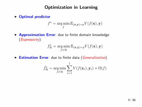
Optimization in Learning
I Optimal predictor
f = arg minf
E(xy)simpV (f(x)y)
I Approximation Error due to finite domain knowledge(Expressivity)
fH = arg minfisinH
E(xy)simpV (f(x)y)
I Estimation Error due to finite data (Generalization)
fH = arg minfisinH
lsumi=1
V (f(xi)yi) + Ω(f)
I Optimization Error finite computation (Optimization Landscape)
return f(i)H
Tractable but bad model or intractable but good model
5 36
Optimization in Learning
I Optimal predictor
f = arg minf
E(xy)simpV (f(x)y)
I Approximation Error due to finite domain knowledge(Expressivity)
fH = arg minfisinH
E(xy)simpV (f(x)y)
I Estimation Error due to finite data (Generalization)
fH = arg minfisinH
lsumi=1
V (f(xi)yi) + Ω(f)
I Optimization Error finite computation (Optimization Landscape)
return f(i)H
Tractable but bad model or intractable but good model
5 36
Optimization in Learning
I Optimal predictor
f = arg minf
E(xy)simpV (f(x)y)
I Approximation Error due to finite domain knowledge(Expressivity)
fH = arg minfisinH
E(xy)simpV (f(x)y)
I Estimation Error due to finite data (Generalization)
fH = arg minfisinH
lsumi=1
V (f(xi)yi) + Ω(f)
I Optimization Error finite computation (Optimization Landscape)
return f(i)H
Tractable but bad model or intractable but good model 5 36
Nonlinearities Everywhere
Large l =rArr Big models H ldquorichrdquo non-parametricnonlinear
6 36
Nonlinearities Everywhere
Large l =rArr Big models H ldquorichrdquo non-parametricnonlinear
6 36
Nonlinearities Everywhere
Large l =rArr Big models H ldquorichrdquo non-parametricnonlinear
6 36
Choice of Nonlinear Hypothesis Space Kernels
x Ψ wTΨ(x) y
w
Ψ(x)
I eg Linear functions and Polynomials
I Infinite-dimensional nonlinear embeddings Fully non-parameteric
I Functional Analysis (Aronszajn Bergman (1950s)) Statistics (Parzen(1960s)) PDEs Numerical Analysis
I ML in 1990rsquos Nonlinear classification regression clustering time-seriesanalysis dynamical systems hypothesis testing causal modeling
I Convex Optimization
7 36
Choice of Nonlinear Hypothesis Space Kernels
x Ψ wTΨ(x) y
w
Ψ(x)
I eg Linear functions and Polynomials
I Infinite-dimensional nonlinear embeddings Fully non-parameteric
I Functional Analysis (Aronszajn Bergman (1950s)) Statistics (Parzen(1960s)) PDEs Numerical Analysis
I ML in 1990rsquos Nonlinear classification regression clustering time-seriesanalysis dynamical systems hypothesis testing causal modeling
I Convex Optimization
7 36
Choice of Nonlinear Hypothesis Space Kernels
x Ψ wTΨ(x) y
w
Ψ(x)
I eg Linear functions and Polynomials
I Infinite-dimensional nonlinear embeddings Fully non-parameteric
I Functional Analysis (Aronszajn Bergman (1950s)) Statistics (Parzen(1960s)) PDEs Numerical Analysis
I ML in 1990rsquos Nonlinear classification regression clustering time-seriesanalysis dynamical systems hypothesis testing causal modeling
I Convex Optimization
7 36
Choice of Nonlinear Hypothesis Space Kernels
x Ψ wTΨ(x) y
w
Ψ(x)
I eg Linear functions and Polynomials
I Infinite-dimensional nonlinear embeddings Fully non-parameteric
I Functional Analysis (Aronszajn Bergman (1950s)) Statistics (Parzen(1960s)) PDEs Numerical Analysis
I ML in 1990rsquos Nonlinear classification regression clustering time-seriesanalysis dynamical systems hypothesis testing causal modeling
I Convex Optimization
7 36
Choice of Nonlinear Hypothesis Space Kernels
x Ψ wTΨ(x) y
w
Ψ(x)
I eg Linear functions and Polynomials
I Infinite-dimensional nonlinear embeddings Fully non-parameteric
I Functional Analysis (Aronszajn Bergman (1950s)) Statistics (Parzen(1960s)) PDEs Numerical Analysis
I ML in 1990rsquos Nonlinear classification regression clustering time-seriesanalysis dynamical systems hypothesis testing causal modeling
I Convex Optimization
7 36
Choice of Nonlinear Hypothesis Space Deep Learning
x0 f1 f2 fL `
w1 w2 wL
z isin Rx1 x2 xLminus1 xL
I Compositions Raw data to higher abstractions (representation learning)
I Multilayer Perceptrons fl(xW) = σ(Wx) (sigmoids ReLU)I Turing (1950) In considering the functions of the mind or the brain we find certain operations which we can explain in
purely mechanical terms This we say does not correspond to the real mind it is a sort of skin which we must strip off if we are
to find the real mind Proceeding in this way do we ever come to the rdquorealrdquo mind or do we eventually come to the skin which
has nothing in it In the latter case the whole mind is mechanical
I Rosenblatt (1957) NYT 1958 New Navy Device Learns By Doing The Navy revealed the embryo of an electronic
computer today that it expects will be able to walk talk see write reproduce itself and be conscious of its existence Later
perceptrons will be able to recognize people and call out their names and instantly translate speech in one language to speech
and writing in another language it was predicted
I Perceptron (Minski and Pappert 1969) [Olarzan A Sociological Study 1996]I Backprop (1986) Reverse-mode differentiation (1960s-70s) CNNs (1980s 2012-)I Breadth-Width tradeoffsI Non-convex Optimization Domain-agnostic recipe
8 36
Choice of Nonlinear Hypothesis Space Deep Learning
x0 f1 f2 fL `
w1 w2 wL
z isin Rx1 x2 xLminus1 xL
I Compositions Raw data to higher abstractions (representation learning)I Multilayer Perceptrons fl(xW) = σ(Wx) (sigmoids ReLU)
I Turing (1950) In considering the functions of the mind or the brain we find certain operations which we can explain in
purely mechanical terms This we say does not correspond to the real mind it is a sort of skin which we must strip off if we are
to find the real mind Proceeding in this way do we ever come to the rdquorealrdquo mind or do we eventually come to the skin which
has nothing in it In the latter case the whole mind is mechanical
I Rosenblatt (1957) NYT 1958 New Navy Device Learns By Doing The Navy revealed the embryo of an electronic
computer today that it expects will be able to walk talk see write reproduce itself and be conscious of its existence Later
perceptrons will be able to recognize people and call out their names and instantly translate speech in one language to speech
and writing in another language it was predicted
I Perceptron (Minski and Pappert 1969) [Olarzan A Sociological Study 1996]I Backprop (1986) Reverse-mode differentiation (1960s-70s) CNNs (1980s 2012-)I Breadth-Width tradeoffsI Non-convex Optimization Domain-agnostic recipe
8 36
Choice of Nonlinear Hypothesis Space Deep Learning
x0 f1 f2 fL `
w1 w2 wL
z isin Rx1 x2 xLminus1 xL
I Compositions Raw data to higher abstractions (representation learning)I Multilayer Perceptrons fl(xW) = σ(Wx) (sigmoids ReLU)I Turing (1950) In considering the functions of the mind or the brain we find certain operations which we can explain in
purely mechanical terms This we say does not correspond to the real mind it is a sort of skin which we must strip off if we are
to find the real mind Proceeding in this way do we ever come to the rdquorealrdquo mind or do we eventually come to the skin which
has nothing in it In the latter case the whole mind is mechanical
I Rosenblatt (1957) NYT 1958 New Navy Device Learns By Doing The Navy revealed the embryo of an electronic
computer today that it expects will be able to walk talk see write reproduce itself and be conscious of its existence Later
perceptrons will be able to recognize people and call out their names and instantly translate speech in one language to speech
and writing in another language it was predicted
I Perceptron (Minski and Pappert 1969) [Olarzan A Sociological Study 1996]I Backprop (1986) Reverse-mode differentiation (1960s-70s) CNNs (1980s 2012-)I Breadth-Width tradeoffsI Non-convex Optimization Domain-agnostic recipe
8 36
Choice of Nonlinear Hypothesis Space Deep Learning
x0 f1 f2 fL `
w1 w2 wL
z isin Rx1 x2 xLminus1 xL
I Compositions Raw data to higher abstractions (representation learning)I Multilayer Perceptrons fl(xW) = σ(Wx) (sigmoids ReLU)I Turing (1950) In considering the functions of the mind or the brain we find certain operations which we can explain in
purely mechanical terms This we say does not correspond to the real mind it is a sort of skin which we must strip off if we are
to find the real mind Proceeding in this way do we ever come to the rdquorealrdquo mind or do we eventually come to the skin which
has nothing in it In the latter case the whole mind is mechanical
I Rosenblatt (1957) NYT 1958 New Navy Device Learns By Doing The Navy revealed the embryo of an electronic
computer today that it expects will be able to walk talk see write reproduce itself and be conscious of its existence Later
perceptrons will be able to recognize people and call out their names and instantly translate speech in one language to speech
and writing in another language it was predicted
I Perceptron (Minski and Pappert 1969) [Olarzan A Sociological Study 1996]I Backprop (1986) Reverse-mode differentiation (1960s-70s) CNNs (1980s 2012-)I Breadth-Width tradeoffsI Non-convex Optimization Domain-agnostic recipe
8 36
Choice of Nonlinear Hypothesis Space Deep Learning
x0 f1 f2 fL `
w1 w2 wL
z isin Rx1 x2 xLminus1 xL
I Compositions Raw data to higher abstractions (representation learning)I Multilayer Perceptrons fl(xW) = σ(Wx) (sigmoids ReLU)I Turing (1950) In considering the functions of the mind or the brain we find certain operations which we can explain in
purely mechanical terms This we say does not correspond to the real mind it is a sort of skin which we must strip off if we are
to find the real mind Proceeding in this way do we ever come to the rdquorealrdquo mind or do we eventually come to the skin which
has nothing in it In the latter case the whole mind is mechanical
I Rosenblatt (1957) NYT 1958 New Navy Device Learns By Doing The Navy revealed the embryo of an electronic
computer today that it expects will be able to walk talk see write reproduce itself and be conscious of its existence Later
perceptrons will be able to recognize people and call out their names and instantly translate speech in one language to speech
and writing in another language it was predicted
I Perceptron (Minski and Pappert 1969) [Olarzan A Sociological Study 1996]I Backprop (1986) Reverse-mode differentiation (1960s-70s) CNNs (1980s 2012-)
I Breadth-Width tradeoffsI Non-convex Optimization Domain-agnostic recipe
8 36
Choice of Nonlinear Hypothesis Space Deep Learning
x0 f1 f2 fL `
w1 w2 wL
z isin Rx1 x2 xLminus1 xL
I Compositions Raw data to higher abstractions (representation learning)I Multilayer Perceptrons fl(xW) = σ(Wx) (sigmoids ReLU)I Turing (1950) In considering the functions of the mind or the brain we find certain operations which we can explain in
purely mechanical terms This we say does not correspond to the real mind it is a sort of skin which we must strip off if we are
to find the real mind Proceeding in this way do we ever come to the rdquorealrdquo mind or do we eventually come to the skin which
has nothing in it In the latter case the whole mind is mechanical
I Rosenblatt (1957) NYT 1958 New Navy Device Learns By Doing The Navy revealed the embryo of an electronic
computer today that it expects will be able to walk talk see write reproduce itself and be conscious of its existence Later
perceptrons will be able to recognize people and call out their names and instantly translate speech in one language to speech
and writing in another language it was predicted
I Perceptron (Minski and Pappert 1969) [Olarzan A Sociological Study 1996]I Backprop (1986) Reverse-mode differentiation (1960s-70s) CNNs (1980s 2012-)I Breadth-Width tradeoffsI Non-convex Optimization Domain-agnostic recipe 8 36
Choice of Nonlinear Hypothesis Space Deep Learning
x0 f1 f2 fL `
w1 w2 wL
z isin Rx1 x2 xLminus1 xL
I Compositions Raw data to higher abstractions (representation learning)I Multilayer Perceptrons fl(xW) = σ(Wx) (sigmoids ReLU)I Turing (1950) In considering the functions of the mind or the brain we find certain operations which we can explain in
purely mechanical terms This we say does not correspond to the real mind it is a sort of skin which we must strip off if we are
to find the real mind Proceeding in this way do we ever come to the rdquorealrdquo mind or do we eventually come to the skin which
has nothing in it In the latter case the whole mind is mechanical
I Rosenblatt (1957) NYT 1958 New Navy Device Learns By Doing The Navy revealed the embryo of an electronic
computer today that it expects will be able to walk talk see write reproduce itself and be conscious of its existence Later
perceptrons will be able to recognize people and call out their names and instantly translate speech in one language to speech
and writing in another language it was predicted
I Perceptron (Minski and Pappert 1969) [Olarzan A Sociological Study 1996]I Backprop (1986) Reverse-mode differentiation (1960s-70s) CNNs (1980s 2012-)I Breadth-Width tradeoffsI Non-convex Optimization Domain-agnostic recipe 8 36
The Watershed Moment Imagenet 2012
I Many statistical and computational ingredientsndash Large datasets (ILSVRC since 2010)
ndash Large statistical capacity (12M images 60M params)ndash Distributed computationndash Depth Invariant feature learning (transferrable to other tasks)ndash Engineering Dropout ReLU
I Many astonishing results since then
9 36
The Watershed Moment Imagenet 2012
I Many statistical and computational ingredientsndash Large datasets (ILSVRC since 2010)ndash Large statistical capacity (12M images 60M params)
ndash Distributed computationndash Depth Invariant feature learning (transferrable to other tasks)ndash Engineering Dropout ReLU
I Many astonishing results since then
9 36
The Watershed Moment Imagenet 2012
I Many statistical and computational ingredientsndash Large datasets (ILSVRC since 2010)ndash Large statistical capacity (12M images 60M params)ndash Distributed computation
ndash Depth Invariant feature learning (transferrable to other tasks)ndash Engineering Dropout ReLU
I Many astonishing results since then
9 36
The Watershed Moment Imagenet 2012
I Many statistical and computational ingredientsndash Large datasets (ILSVRC since 2010)ndash Large statistical capacity (12M images 60M params)ndash Distributed computationndash Depth Invariant feature learning (transferrable to other tasks)
ndash Engineering Dropout ReLU I Many astonishing results since then
9 36
The Watershed Moment Imagenet 2012
I Many statistical and computational ingredientsndash Large datasets (ILSVRC since 2010)ndash Large statistical capacity (12M images 60M params)ndash Distributed computationndash Depth Invariant feature learning (transferrable to other tasks)ndash Engineering Dropout ReLU
I Many astonishing results since then
9 36
CNNs
10 36
Self-Driving Cars
Figure End-to-End Learning for Self-driving Cars Bojarski et al 2016
11 36

Optimization in Learning
I Optimal predictor
f = arg minf
E(xy)simpV (f(x)y)
I Approximation Error due to finite domain knowledge(Expressivity)
fH = arg minfisinH
E(xy)simpV (f(x)y)
I Estimation Error due to finite data (Generalization)
fH = arg minfisinH
lsumi=1
V (f(xi)yi) + Ω(f)
I Optimization Error finite computation (Optimization Landscape)
return f(i)H
Tractable but bad model or intractable but good model
5 36
Optimization in Learning
I Optimal predictor
f = arg minf
E(xy)simpV (f(x)y)
I Approximation Error due to finite domain knowledge(Expressivity)
fH = arg minfisinH
E(xy)simpV (f(x)y)
I Estimation Error due to finite data (Generalization)
fH = arg minfisinH
lsumi=1
V (f(xi)yi) + Ω(f)
I Optimization Error finite computation (Optimization Landscape)
return f(i)H
Tractable but bad model or intractable but good model 5 36
Nonlinearities Everywhere
Large l =rArr Big models H ldquorichrdquo non-parametricnonlinear
6 36
Nonlinearities Everywhere
Large l =rArr Big models H ldquorichrdquo non-parametricnonlinear
6 36
Nonlinearities Everywhere
Large l =rArr Big models H ldquorichrdquo non-parametricnonlinear
6 36
Choice of Nonlinear Hypothesis Space Kernels
x Ψ wTΨ(x) y
w
Ψ(x)
I eg Linear functions and Polynomials
I Infinite-dimensional nonlinear embeddings Fully non-parameteric
I Functional Analysis (Aronszajn Bergman (1950s)) Statistics (Parzen(1960s)) PDEs Numerical Analysis
I ML in 1990rsquos Nonlinear classification regression clustering time-seriesanalysis dynamical systems hypothesis testing causal modeling
I Convex Optimization
7 36
Choice of Nonlinear Hypothesis Space Kernels
x Ψ wTΨ(x) y
w
Ψ(x)
I eg Linear functions and Polynomials
I Infinite-dimensional nonlinear embeddings Fully non-parameteric
I Functional Analysis (Aronszajn Bergman (1950s)) Statistics (Parzen(1960s)) PDEs Numerical Analysis
I ML in 1990rsquos Nonlinear classification regression clustering time-seriesanalysis dynamical systems hypothesis testing causal modeling
I Convex Optimization
7 36
Choice of Nonlinear Hypothesis Space Kernels
x Ψ wTΨ(x) y
w
Ψ(x)
I eg Linear functions and Polynomials
I Infinite-dimensional nonlinear embeddings Fully non-parameteric
I Functional Analysis (Aronszajn Bergman (1950s)) Statistics (Parzen(1960s)) PDEs Numerical Analysis
I ML in 1990rsquos Nonlinear classification regression clustering time-seriesanalysis dynamical systems hypothesis testing causal modeling
I Convex Optimization
7 36
Choice of Nonlinear Hypothesis Space Kernels
x Ψ wTΨ(x) y
w
Ψ(x)
I eg Linear functions and Polynomials
I Infinite-dimensional nonlinear embeddings Fully non-parameteric
I Functional Analysis (Aronszajn Bergman (1950s)) Statistics (Parzen(1960s)) PDEs Numerical Analysis
I ML in 1990rsquos Nonlinear classification regression clustering time-seriesanalysis dynamical systems hypothesis testing causal modeling
I Convex Optimization
7 36
Choice of Nonlinear Hypothesis Space Kernels
x Ψ wTΨ(x) y
w
Ψ(x)
I eg Linear functions and Polynomials
I Infinite-dimensional nonlinear embeddings Fully non-parameteric
I Functional Analysis (Aronszajn Bergman (1950s)) Statistics (Parzen(1960s)) PDEs Numerical Analysis
I ML in 1990rsquos Nonlinear classification regression clustering time-seriesanalysis dynamical systems hypothesis testing causal modeling
I Convex Optimization
7 36
Choice of Nonlinear Hypothesis Space Deep Learning
x0 f1 f2 fL `
w1 w2 wL
z isin Rx1 x2 xLminus1 xL
I Compositions Raw data to higher abstractions (representation learning)
I Multilayer Perceptrons fl(xW) = σ(Wx) (sigmoids ReLU)I Turing (1950) In considering the functions of the mind or the brain we find certain operations which we can explain in
purely mechanical terms This we say does not correspond to the real mind it is a sort of skin which we must strip off if we are
to find the real mind Proceeding in this way do we ever come to the rdquorealrdquo mind or do we eventually come to the skin which
has nothing in it In the latter case the whole mind is mechanical
I Rosenblatt (1957) NYT 1958 New Navy Device Learns By Doing The Navy revealed the embryo of an electronic
computer today that it expects will be able to walk talk see write reproduce itself and be conscious of its existence Later
perceptrons will be able to recognize people and call out their names and instantly translate speech in one language to speech
and writing in another language it was predicted
I Perceptron (Minski and Pappert 1969) [Olarzan A Sociological Study 1996]I Backprop (1986) Reverse-mode differentiation (1960s-70s) CNNs (1980s 2012-)I Breadth-Width tradeoffsI Non-convex Optimization Domain-agnostic recipe
8 36
Choice of Nonlinear Hypothesis Space Deep Learning
x0 f1 f2 fL `
w1 w2 wL
z isin Rx1 x2 xLminus1 xL
I Compositions Raw data to higher abstractions (representation learning)I Multilayer Perceptrons fl(xW) = σ(Wx) (sigmoids ReLU)
I Turing (1950) In considering the functions of the mind or the brain we find certain operations which we can explain in
purely mechanical terms This we say does not correspond to the real mind it is a sort of skin which we must strip off if we are
to find the real mind Proceeding in this way do we ever come to the rdquorealrdquo mind or do we eventually come to the skin which
has nothing in it In the latter case the whole mind is mechanical
I Rosenblatt (1957) NYT 1958 New Navy Device Learns By Doing The Navy revealed the embryo of an electronic
computer today that it expects will be able to walk talk see write reproduce itself and be conscious of its existence Later
perceptrons will be able to recognize people and call out their names and instantly translate speech in one language to speech
and writing in another language it was predicted
I Perceptron (Minski and Pappert 1969) [Olarzan A Sociological Study 1996]I Backprop (1986) Reverse-mode differentiation (1960s-70s) CNNs (1980s 2012-)I Breadth-Width tradeoffsI Non-convex Optimization Domain-agnostic recipe
8 36
Choice of Nonlinear Hypothesis Space Deep Learning
x0 f1 f2 fL `
w1 w2 wL
z isin Rx1 x2 xLminus1 xL
I Compositions Raw data to higher abstractions (representation learning)I Multilayer Perceptrons fl(xW) = σ(Wx) (sigmoids ReLU)I Turing (1950) In considering the functions of the mind or the brain we find certain operations which we can explain in
purely mechanical terms This we say does not correspond to the real mind it is a sort of skin which we must strip off if we are
to find the real mind Proceeding in this way do we ever come to the rdquorealrdquo mind or do we eventually come to the skin which
has nothing in it In the latter case the whole mind is mechanical
I Rosenblatt (1957) NYT 1958 New Navy Device Learns By Doing The Navy revealed the embryo of an electronic
computer today that it expects will be able to walk talk see write reproduce itself and be conscious of its existence Later
perceptrons will be able to recognize people and call out their names and instantly translate speech in one language to speech
and writing in another language it was predicted
I Perceptron (Minski and Pappert 1969) [Olarzan A Sociological Study 1996]I Backprop (1986) Reverse-mode differentiation (1960s-70s) CNNs (1980s 2012-)I Breadth-Width tradeoffsI Non-convex Optimization Domain-agnostic recipe
8 36
Choice of Nonlinear Hypothesis Space Deep Learning
x0 f1 f2 fL `
w1 w2 wL
z isin Rx1 x2 xLminus1 xL
I Compositions Raw data to higher abstractions (representation learning)I Multilayer Perceptrons fl(xW) = σ(Wx) (sigmoids ReLU)I Turing (1950) In considering the functions of the mind or the brain we find certain operations which we can explain in
purely mechanical terms This we say does not correspond to the real mind it is a sort of skin which we must strip off if we are
to find the real mind Proceeding in this way do we ever come to the rdquorealrdquo mind or do we eventually come to the skin which
has nothing in it In the latter case the whole mind is mechanical
I Rosenblatt (1957) NYT 1958 New Navy Device Learns By Doing The Navy revealed the embryo of an electronic
computer today that it expects will be able to walk talk see write reproduce itself and be conscious of its existence Later
perceptrons will be able to recognize people and call out their names and instantly translate speech in one language to speech
and writing in another language it was predicted
I Perceptron (Minski and Pappert 1969) [Olarzan A Sociological Study 1996]I Backprop (1986) Reverse-mode differentiation (1960s-70s) CNNs (1980s 2012-)I Breadth-Width tradeoffsI Non-convex Optimization Domain-agnostic recipe
8 36
Choice of Nonlinear Hypothesis Space Deep Learning
x0 f1 f2 fL `
w1 w2 wL
z isin Rx1 x2 xLminus1 xL
I Compositions Raw data to higher abstractions (representation learning)I Multilayer Perceptrons fl(xW) = σ(Wx) (sigmoids ReLU)I Turing (1950) In considering the functions of the mind or the brain we find certain operations which we can explain in
purely mechanical terms This we say does not correspond to the real mind it is a sort of skin which we must strip off if we are
to find the real mind Proceeding in this way do we ever come to the rdquorealrdquo mind or do we eventually come to the skin which
has nothing in it In the latter case the whole mind is mechanical
I Rosenblatt (1957) NYT 1958 New Navy Device Learns By Doing The Navy revealed the embryo of an electronic
computer today that it expects will be able to walk talk see write reproduce itself and be conscious of its existence Later
perceptrons will be able to recognize people and call out their names and instantly translate speech in one language to speech
and writing in another language it was predicted
I Perceptron (Minski and Pappert 1969) [Olarzan A Sociological Study 1996]I Backprop (1986) Reverse-mode differentiation (1960s-70s) CNNs (1980s 2012-)
I Breadth-Width tradeoffsI Non-convex Optimization Domain-agnostic recipe
8 36
Choice of Nonlinear Hypothesis Space Deep Learning
x0 f1 f2 fL `
w1 w2 wL
z isin Rx1 x2 xLminus1 xL
I Compositions Raw data to higher abstractions (representation learning)I Multilayer Perceptrons fl(xW) = σ(Wx) (sigmoids ReLU)I Turing (1950) In considering the functions of the mind or the brain we find certain operations which we can explain in
purely mechanical terms This we say does not correspond to the real mind it is a sort of skin which we must strip off if we are
to find the real mind Proceeding in this way do we ever come to the rdquorealrdquo mind or do we eventually come to the skin which
has nothing in it In the latter case the whole mind is mechanical
I Rosenblatt (1957) NYT 1958 New Navy Device Learns By Doing The Navy revealed the embryo of an electronic
computer today that it expects will be able to walk talk see write reproduce itself and be conscious of its existence Later
perceptrons will be able to recognize people and call out their names and instantly translate speech in one language to speech
and writing in another language it was predicted
I Perceptron (Minski and Pappert 1969) [Olarzan A Sociological Study 1996]I Backprop (1986) Reverse-mode differentiation (1960s-70s) CNNs (1980s 2012-)I Breadth-Width tradeoffsI Non-convex Optimization Domain-agnostic recipe 8 36
Choice of Nonlinear Hypothesis Space Deep Learning
x0 f1 f2 fL `
w1 w2 wL
z isin Rx1 x2 xLminus1 xL
I Compositions Raw data to higher abstractions (representation learning)I Multilayer Perceptrons fl(xW) = σ(Wx) (sigmoids ReLU)I Turing (1950) In considering the functions of the mind or the brain we find certain operations which we can explain in
purely mechanical terms This we say does not correspond to the real mind it is a sort of skin which we must strip off if we are
to find the real mind Proceeding in this way do we ever come to the rdquorealrdquo mind or do we eventually come to the skin which
has nothing in it In the latter case the whole mind is mechanical
I Rosenblatt (1957) NYT 1958 New Navy Device Learns By Doing The Navy revealed the embryo of an electronic
computer today that it expects will be able to walk talk see write reproduce itself and be conscious of its existence Later
perceptrons will be able to recognize people and call out their names and instantly translate speech in one language to speech
and writing in another language it was predicted
I Perceptron (Minski and Pappert 1969) [Olarzan A Sociological Study 1996]I Backprop (1986) Reverse-mode differentiation (1960s-70s) CNNs (1980s 2012-)I Breadth-Width tradeoffsI Non-convex Optimization Domain-agnostic recipe 8 36
The Watershed Moment Imagenet 2012
I Many statistical and computational ingredientsndash Large datasets (ILSVRC since 2010)
ndash Large statistical capacity (12M images 60M params)ndash Distributed computationndash Depth Invariant feature learning (transferrable to other tasks)ndash Engineering Dropout ReLU
I Many astonishing results since then
9 36
The Watershed Moment Imagenet 2012
I Many statistical and computational ingredientsndash Large datasets (ILSVRC since 2010)ndash Large statistical capacity (12M images 60M params)
ndash Distributed computationndash Depth Invariant feature learning (transferrable to other tasks)ndash Engineering Dropout ReLU
I Many astonishing results since then
9 36
The Watershed Moment Imagenet 2012
I Many statistical and computational ingredientsndash Large datasets (ILSVRC since 2010)ndash Large statistical capacity (12M images 60M params)ndash Distributed computation
ndash Depth Invariant feature learning (transferrable to other tasks)ndash Engineering Dropout ReLU
I Many astonishing results since then
9 36
The Watershed Moment Imagenet 2012
I Many statistical and computational ingredientsndash Large datasets (ILSVRC since 2010)ndash Large statistical capacity (12M images 60M params)ndash Distributed computationndash Depth Invariant feature learning (transferrable to other tasks)
ndash Engineering Dropout ReLU I Many astonishing results since then
9 36
The Watershed Moment Imagenet 2012
I Many statistical and computational ingredientsndash Large datasets (ILSVRC since 2010)ndash Large statistical capacity (12M images 60M params)ndash Distributed computationndash Depth Invariant feature learning (transferrable to other tasks)ndash Engineering Dropout ReLU
I Many astonishing results since then
9 36
CNNs
10 36
Self-Driving Cars
Figure End-to-End Learning for Self-driving Cars Bojarski et al 2016
11 36

Optimization in Learning
I Optimal predictor
f = arg minf
E(xy)simpV (f(x)y)
I Approximation Error due to finite domain knowledge(Expressivity)
fH = arg minfisinH
E(xy)simpV (f(x)y)
I Estimation Error due to finite data (Generalization)
fH = arg minfisinH
lsumi=1
V (f(xi)yi) + Ω(f)
I Optimization Error finite computation (Optimization Landscape)
return f(i)H
Tractable but bad model or intractable but good model 5 36
Nonlinearities Everywhere
Large l =rArr Big models H ldquorichrdquo non-parametricnonlinear
6 36
Nonlinearities Everywhere
Large l =rArr Big models H ldquorichrdquo non-parametricnonlinear
6 36
Nonlinearities Everywhere
Large l =rArr Big models H ldquorichrdquo non-parametricnonlinear
6 36
Choice of Nonlinear Hypothesis Space Kernels
x Ψ wTΨ(x) y
w
Ψ(x)
I eg Linear functions and Polynomials
I Infinite-dimensional nonlinear embeddings Fully non-parameteric
I Functional Analysis (Aronszajn Bergman (1950s)) Statistics (Parzen(1960s)) PDEs Numerical Analysis
I ML in 1990rsquos Nonlinear classification regression clustering time-seriesanalysis dynamical systems hypothesis testing causal modeling
I Convex Optimization
7 36
Choice of Nonlinear Hypothesis Space Kernels
x Ψ wTΨ(x) y
w
Ψ(x)
I eg Linear functions and Polynomials
I Infinite-dimensional nonlinear embeddings Fully non-parameteric
I Functional Analysis (Aronszajn Bergman (1950s)) Statistics (Parzen(1960s)) PDEs Numerical Analysis
I ML in 1990rsquos Nonlinear classification regression clustering time-seriesanalysis dynamical systems hypothesis testing causal modeling
I Convex Optimization
7 36
Choice of Nonlinear Hypothesis Space Kernels
x Ψ wTΨ(x) y
w
Ψ(x)
I eg Linear functions and Polynomials
I Infinite-dimensional nonlinear embeddings Fully non-parameteric
I Functional Analysis (Aronszajn Bergman (1950s)) Statistics (Parzen(1960s)) PDEs Numerical Analysis
I ML in 1990rsquos Nonlinear classification regression clustering time-seriesanalysis dynamical systems hypothesis testing causal modeling
I Convex Optimization
7 36
Choice of Nonlinear Hypothesis Space Kernels
x Ψ wTΨ(x) y
w
Ψ(x)
I eg Linear functions and Polynomials
I Infinite-dimensional nonlinear embeddings Fully non-parameteric
I Functional Analysis (Aronszajn Bergman (1950s)) Statistics (Parzen(1960s)) PDEs Numerical Analysis
I ML in 1990rsquos Nonlinear classification regression clustering time-seriesanalysis dynamical systems hypothesis testing causal modeling
I Convex Optimization
7 36
Choice of Nonlinear Hypothesis Space Kernels
x Ψ wTΨ(x) y
w
Ψ(x)
I eg Linear functions and Polynomials
I Infinite-dimensional nonlinear embeddings Fully non-parameteric
I Functional Analysis (Aronszajn Bergman (1950s)) Statistics (Parzen(1960s)) PDEs Numerical Analysis
I ML in 1990rsquos Nonlinear classification regression clustering time-seriesanalysis dynamical systems hypothesis testing causal modeling
I Convex Optimization
7 36
Choice of Nonlinear Hypothesis Space Deep Learning
x0 f1 f2 fL `
w1 w2 wL
z isin Rx1 x2 xLminus1 xL
I Compositions Raw data to higher abstractions (representation learning)
I Multilayer Perceptrons fl(xW) = σ(Wx) (sigmoids ReLU)I Turing (1950) In considering the functions of the mind or the brain we find certain operations which we can explain in
purely mechanical terms This we say does not correspond to the real mind it is a sort of skin which we must strip off if we are
to find the real mind Proceeding in this way do we ever come to the rdquorealrdquo mind or do we eventually come to the skin which
has nothing in it In the latter case the whole mind is mechanical
I Rosenblatt (1957) NYT 1958 New Navy Device Learns By Doing The Navy revealed the embryo of an electronic
computer today that it expects will be able to walk talk see write reproduce itself and be conscious of its existence Later
perceptrons will be able to recognize people and call out their names and instantly translate speech in one language to speech
and writing in another language it was predicted
I Perceptron (Minski and Pappert 1969) [Olarzan A Sociological Study 1996]I Backprop (1986) Reverse-mode differentiation (1960s-70s) CNNs (1980s 2012-)I Breadth-Width tradeoffsI Non-convex Optimization Domain-agnostic recipe
8 36
Choice of Nonlinear Hypothesis Space Deep Learning
x0 f1 f2 fL `
w1 w2 wL
z isin Rx1 x2 xLminus1 xL
I Compositions Raw data to higher abstractions (representation learning)I Multilayer Perceptrons fl(xW) = σ(Wx) (sigmoids ReLU)
I Turing (1950) In considering the functions of the mind or the brain we find certain operations which we can explain in
purely mechanical terms This we say does not correspond to the real mind it is a sort of skin which we must strip off if we are
to find the real mind Proceeding in this way do we ever come to the rdquorealrdquo mind or do we eventually come to the skin which
has nothing in it In the latter case the whole mind is mechanical
I Rosenblatt (1957) NYT 1958 New Navy Device Learns By Doing The Navy revealed the embryo of an electronic
computer today that it expects will be able to walk talk see write reproduce itself and be conscious of its existence Later
perceptrons will be able to recognize people and call out their names and instantly translate speech in one language to speech
and writing in another language it was predicted
I Perceptron (Minski and Pappert 1969) [Olarzan A Sociological Study 1996]I Backprop (1986) Reverse-mode differentiation (1960s-70s) CNNs (1980s 2012-)I Breadth-Width tradeoffsI Non-convex Optimization Domain-agnostic recipe
8 36
Choice of Nonlinear Hypothesis Space Deep Learning
x0 f1 f2 fL `
w1 w2 wL
z isin Rx1 x2 xLminus1 xL
I Compositions Raw data to higher abstractions (representation learning)I Multilayer Perceptrons fl(xW) = σ(Wx) (sigmoids ReLU)I Turing (1950) In considering the functions of the mind or the brain we find certain operations which we can explain in
purely mechanical terms This we say does not correspond to the real mind it is a sort of skin which we must strip off if we are
to find the real mind Proceeding in this way do we ever come to the rdquorealrdquo mind or do we eventually come to the skin which
has nothing in it In the latter case the whole mind is mechanical
I Rosenblatt (1957) NYT 1958 New Navy Device Learns By Doing The Navy revealed the embryo of an electronic
computer today that it expects will be able to walk talk see write reproduce itself and be conscious of its existence Later
perceptrons will be able to recognize people and call out their names and instantly translate speech in one language to speech
and writing in another language it was predicted
I Perceptron (Minski and Pappert 1969) [Olarzan A Sociological Study 1996]I Backprop (1986) Reverse-mode differentiation (1960s-70s) CNNs (1980s 2012-)I Breadth-Width tradeoffsI Non-convex Optimization Domain-agnostic recipe
8 36
Choice of Nonlinear Hypothesis Space Deep Learning
x0 f1 f2 fL `
w1 w2 wL
z isin Rx1 x2 xLminus1 xL
I Compositions Raw data to higher abstractions (representation learning)I Multilayer Perceptrons fl(xW) = σ(Wx) (sigmoids ReLU)I Turing (1950) In considering the functions of the mind or the brain we find certain operations which we can explain in
purely mechanical terms This we say does not correspond to the real mind it is a sort of skin which we must strip off if we are
to find the real mind Proceeding in this way do we ever come to the rdquorealrdquo mind or do we eventually come to the skin which
has nothing in it In the latter case the whole mind is mechanical
I Rosenblatt (1957) NYT 1958 New Navy Device Learns By Doing The Navy revealed the embryo of an electronic
computer today that it expects will be able to walk talk see write reproduce itself and be conscious of its existence Later
perceptrons will be able to recognize people and call out their names and instantly translate speech in one language to speech
and writing in another language it was predicted
I Perceptron (Minski and Pappert 1969) [Olarzan A Sociological Study 1996]I Backprop (1986) Reverse-mode differentiation (1960s-70s) CNNs (1980s 2012-)I Breadth-Width tradeoffsI Non-convex Optimization Domain-agnostic recipe
8 36
Choice of Nonlinear Hypothesis Space Deep Learning
x0 f1 f2 fL `
w1 w2 wL
z isin Rx1 x2 xLminus1 xL
I Compositions Raw data to higher abstractions (representation learning)I Multilayer Perceptrons fl(xW) = σ(Wx) (sigmoids ReLU)I Turing (1950) In considering the functions of the mind or the brain we find certain operations which we can explain in
purely mechanical terms This we say does not correspond to the real mind it is a sort of skin which we must strip off if we are
to find the real mind Proceeding in this way do we ever come to the rdquorealrdquo mind or do we eventually come to the skin which
has nothing in it In the latter case the whole mind is mechanical
I Rosenblatt (1957) NYT 1958 New Navy Device Learns By Doing The Navy revealed the embryo of an electronic
computer today that it expects will be able to walk talk see write reproduce itself and be conscious of its existence Later
perceptrons will be able to recognize people and call out their names and instantly translate speech in one language to speech
and writing in another language it was predicted
I Perceptron (Minski and Pappert 1969) [Olarzan A Sociological Study 1996]I Backprop (1986) Reverse-mode differentiation (1960s-70s) CNNs (1980s 2012-)
I Breadth-Width tradeoffsI Non-convex Optimization Domain-agnostic recipe
8 36
Choice of Nonlinear Hypothesis Space Deep Learning
x0 f1 f2 fL `
w1 w2 wL
z isin Rx1 x2 xLminus1 xL
I Compositions Raw data to higher abstractions (representation learning)I Multilayer Perceptrons fl(xW) = σ(Wx) (sigmoids ReLU)I Turing (1950) In considering the functions of the mind or the brain we find certain operations which we can explain in
purely mechanical terms This we say does not correspond to the real mind it is a sort of skin which we must strip off if we are
to find the real mind Proceeding in this way do we ever come to the rdquorealrdquo mind or do we eventually come to the skin which
has nothing in it In the latter case the whole mind is mechanical
I Rosenblatt (1957) NYT 1958 New Navy Device Learns By Doing The Navy revealed the embryo of an electronic
computer today that it expects will be able to walk talk see write reproduce itself and be conscious of its existence Later
perceptrons will be able to recognize people and call out their names and instantly translate speech in one language to speech
and writing in another language it was predicted
I Perceptron (Minski and Pappert 1969) [Olarzan A Sociological Study 1996]I Backprop (1986) Reverse-mode differentiation (1960s-70s) CNNs (1980s 2012-)I Breadth-Width tradeoffsI Non-convex Optimization Domain-agnostic recipe 8 36
Choice of Nonlinear Hypothesis Space Deep Learning
x0 f1 f2 fL `
w1 w2 wL
z isin Rx1 x2 xLminus1 xL
I Compositions Raw data to higher abstractions (representation learning)I Multilayer Perceptrons fl(xW) = σ(Wx) (sigmoids ReLU)I Turing (1950) In considering the functions of the mind or the brain we find certain operations which we can explain in
purely mechanical terms This we say does not correspond to the real mind it is a sort of skin which we must strip off if we are
to find the real mind Proceeding in this way do we ever come to the rdquorealrdquo mind or do we eventually come to the skin which
has nothing in it In the latter case the whole mind is mechanical
I Rosenblatt (1957) NYT 1958 New Navy Device Learns By Doing The Navy revealed the embryo of an electronic
computer today that it expects will be able to walk talk see write reproduce itself and be conscious of its existence Later
perceptrons will be able to recognize people and call out their names and instantly translate speech in one language to speech
and writing in another language it was predicted
I Perceptron (Minski and Pappert 1969) [Olarzan A Sociological Study 1996]I Backprop (1986) Reverse-mode differentiation (1960s-70s) CNNs (1980s 2012-)I Breadth-Width tradeoffsI Non-convex Optimization Domain-agnostic recipe 8 36
The Watershed Moment Imagenet 2012
I Many statistical and computational ingredientsndash Large datasets (ILSVRC since 2010)
ndash Large statistical capacity (12M images 60M params)ndash Distributed computationndash Depth Invariant feature learning (transferrable to other tasks)ndash Engineering Dropout ReLU
I Many astonishing results since then
9 36
The Watershed Moment Imagenet 2012
I Many statistical and computational ingredientsndash Large datasets (ILSVRC since 2010)ndash Large statistical capacity (12M images 60M params)
ndash Distributed computationndash Depth Invariant feature learning (transferrable to other tasks)ndash Engineering Dropout ReLU
I Many astonishing results since then
9 36
The Watershed Moment Imagenet 2012
I Many statistical and computational ingredientsndash Large datasets (ILSVRC since 2010)ndash Large statistical capacity (12M images 60M params)ndash Distributed computation
ndash Depth Invariant feature learning (transferrable to other tasks)ndash Engineering Dropout ReLU
I Many astonishing results since then
9 36
The Watershed Moment Imagenet 2012
I Many statistical and computational ingredientsndash Large datasets (ILSVRC since 2010)ndash Large statistical capacity (12M images 60M params)ndash Distributed computationndash Depth Invariant feature learning (transferrable to other tasks)
ndash Engineering Dropout ReLU I Many astonishing results since then
9 36
The Watershed Moment Imagenet 2012
I Many statistical and computational ingredientsndash Large datasets (ILSVRC since 2010)ndash Large statistical capacity (12M images 60M params)ndash Distributed computationndash Depth Invariant feature learning (transferrable to other tasks)ndash Engineering Dropout ReLU
I Many astonishing results since then
9 36
CNNs
10 36
Self-Driving Cars
Figure End-to-End Learning for Self-driving Cars Bojarski et al 2016
11 36

Nonlinearities Everywhere
Large l =rArr Big models H ldquorichrdquo non-parametricnonlinear
6 36
Nonlinearities Everywhere
Large l =rArr Big models H ldquorichrdquo non-parametricnonlinear
6 36
Nonlinearities Everywhere
Large l =rArr Big models H ldquorichrdquo non-parametricnonlinear
6 36
Choice of Nonlinear Hypothesis Space Kernels
x Ψ wTΨ(x) y
w
Ψ(x)
I eg Linear functions and Polynomials
I Infinite-dimensional nonlinear embeddings Fully non-parameteric
I Functional Analysis (Aronszajn Bergman (1950s)) Statistics (Parzen(1960s)) PDEs Numerical Analysis
I ML in 1990rsquos Nonlinear classification regression clustering time-seriesanalysis dynamical systems hypothesis testing causal modeling
I Convex Optimization
7 36
Choice of Nonlinear Hypothesis Space Deep Learning
x0 f1 f2 fL `
w1 w2 wL
z isin Rx1 x2 xLminus1 xL
I Compositions Raw data to higher abstractions (representation learning)
I Multilayer Perceptrons fl(xW) = σ(Wx) (sigmoids ReLU)I Turing (1950) In considering the functions of the mind or the brain we find certain operations which we can explain in
purely mechanical terms This we say does not correspond to the real mind it is a sort of skin which we must strip off if we are
to find the real mind Proceeding in this way do we ever come to the rdquorealrdquo mind or do we eventually come to the skin which
has nothing in it In the latter case the whole mind is mechanical
I Rosenblatt (1957) NYT 1958 New Navy Device Learns By Doing The Navy revealed the embryo of an electronic
computer today that it expects will be able to walk talk see write reproduce itself and be conscious of its existence Later
perceptrons will be able to recognize people and call out their names and instantly translate speech in one language to speech
and writing in another language it was predicted
I Perceptron (Minski and Pappert 1969) [Olarzan A Sociological Study 1996]I Backprop (1986) Reverse-mode differentiation (1960s-70s) CNNs (1980s 2012-)I Breadth-Width tradeoffsI Non-convex Optimization Domain-agnostic recipe
8 36
Choice of Nonlinear Hypothesis Space Deep Learning
x0 f1 f2 fL `
w1 w2 wL
z isin Rx1 x2 xLminus1 xL
I Compositions Raw data to higher abstractions (representation learning)I Multilayer Perceptrons fl(xW) = σ(Wx) (sigmoids ReLU)
I Turing (1950) In considering the functions of the mind or the brain we find certain operations which we can explain in
purely mechanical terms This we say does not correspond to the real mind it is a sort of skin which we must strip off if we are
to find the real mind Proceeding in this way do we ever come to the rdquorealrdquo mind or do we eventually come to the skin which
has nothing in it In the latter case the whole mind is mechanical
I Rosenblatt (1957) NYT 1958 New Navy Device Learns By Doing The Navy revealed the embryo of an electronic
computer today that it expects will be able to walk talk see write reproduce itself and be conscious of its existence Later
perceptrons will be able to recognize people and call out their names and instantly translate speech in one language to speech
and writing in another language it was predicted
I Perceptron (Minski and Pappert 1969) [Olarzan A Sociological Study 1996]I Backprop (1986) Reverse-mode differentiation (1960s-70s) CNNs (1980s 2012-)I Breadth-Width tradeoffsI Non-convex Optimization Domain-agnostic recipe
8 36
Choice of Nonlinear Hypothesis Space Deep Learning
x0 f1 f2 fL `
w1 w2 wL
z isin Rx1 x2 xLminus1 xL
I Compositions Raw data to higher abstractions (representation learning)I Multilayer Perceptrons fl(xW) = σ(Wx) (sigmoids ReLU)I Turing (1950) In considering the functions of the mind or the brain we find certain operations which we can explain in
purely mechanical terms This we say does not correspond to the real mind it is a sort of skin which we must strip off if we are
to find the real mind Proceeding in this way do we ever come to the rdquorealrdquo mind or do we eventually come to the skin which
has nothing in it In the latter case the whole mind is mechanical
I Rosenblatt (1957) NYT 1958 New Navy Device Learns By Doing The Navy revealed the embryo of an electronic
computer today that it expects will be able to walk talk see write reproduce itself and be conscious of its existence Later
perceptrons will be able to recognize people and call out their names and instantly translate speech in one language to speech
and writing in another language it was predicted
I Perceptron (Minski and Pappert 1969) [Olarzan A Sociological Study 1996]I Backprop (1986) Reverse-mode differentiation (1960s-70s) CNNs (1980s 2012-)I Breadth-Width tradeoffsI Non-convex Optimization Domain-agnostic recipe
8 36
Choice of Nonlinear Hypothesis Space Deep Learning
x0 f1 f2 fL `
w1 w2 wL
z isin Rx1 x2 xLminus1 xL
I Compositions Raw data to higher abstractions (representation learning)I Multilayer Perceptrons fl(xW) = σ(Wx) (sigmoids ReLU)I Turing (1950) In considering the functions of the mind or the brain we find certain operations which we can explain in
purely mechanical terms This we say does not correspond to the real mind it is a sort of skin which we must strip off if we are
to find the real mind Proceeding in this way do we ever come to the rdquorealrdquo mind or do we eventually come to the skin which
has nothing in it In the latter case the whole mind is mechanical
I Rosenblatt (1957) NYT 1958 New Navy Device Learns By Doing The Navy revealed the embryo of an electronic
computer today that it expects will be able to walk talk see write reproduce itself and be conscious of its existence Later
perceptrons will be able to recognize people and call out their names and instantly translate speech in one language to speech
and writing in another language it was predicted
I Perceptron (Minski and Pappert 1969) [Olarzan A Sociological Study 1996]I Backprop (1986) Reverse-mode differentiation (1960s-70s) CNNs (1980s 2012-)I Breadth-Width tradeoffsI Non-convex Optimization Domain-agnostic recipe
8 36
Choice of Nonlinear Hypothesis Space Deep Learning
x0 f1 f2 fL `
w1 w2 wL
z isin Rx1 x2 xLminus1 xL
I Compositions Raw data to higher abstractions (representation learning)I Multilayer Perceptrons fl(xW) = σ(Wx) (sigmoids ReLU)I Turing (1950) In considering the functions of the mind or the brain we find certain operations which we can explain in
purely mechanical terms This we say does not correspond to the real mind it is a sort of skin which we must strip off if we are
to find the real mind Proceeding in this way do we ever come to the rdquorealrdquo mind or do we eventually come to the skin which
has nothing in it In the latter case the whole mind is mechanical
I Rosenblatt (1957) NYT 1958 New Navy Device Learns By Doing The Navy revealed the embryo of an electronic
computer today that it expects will be able to walk talk see write reproduce itself and be conscious of its existence Later
perceptrons will be able to recognize people and call out their names and instantly translate speech in one language to speech
and writing in another language it was predicted
I Perceptron (Minski and Pappert 1969) [Olarzan A Sociological Study 1996]I Backprop (1986) Reverse-mode differentiation (1960s-70s) CNNs (1980s 2012-)
I Breadth-Width tradeoffsI Non-convex Optimization Domain-agnostic recipe
8 36
Choice of Nonlinear Hypothesis Space Deep Learning
x0 f1 f2 fL `
w1 w2 wL
z isin Rx1 x2 xLminus1 xL
I Compositions Raw data to higher abstractions (representation learning)I Multilayer Perceptrons fl(xW) = σ(Wx) (sigmoids ReLU)I Turing (1950) In considering the functions of the mind or the brain we find certain operations which we can explain in
purely mechanical terms This we say does not correspond to the real mind it is a sort of skin which we must strip off if we are
to find the real mind Proceeding in this way do we ever come to the rdquorealrdquo mind or do we eventually come to the skin which
has nothing in it In the latter case the whole mind is mechanical
I Rosenblatt (1957) NYT 1958 New Navy Device Learns By Doing The Navy revealed the embryo of an electronic
computer today that it expects will be able to walk talk see write reproduce itself and be conscious of its existence Later
perceptrons will be able to recognize people and call out their names and instantly translate speech in one language to speech
and writing in another language it was predicted
I Perceptron (Minski and Pappert 1969) [Olarzan A Sociological Study 1996]I Backprop (1986) Reverse-mode differentiation (1960s-70s) CNNs (1980s 2012-)I Breadth-Width tradeoffsI Non-convex Optimization Domain-agnostic recipe 8 36
Choice of Nonlinear Hypothesis Space Deep Learning
x0 f1 f2 fL `
w1 w2 wL
z isin Rx1 x2 xLminus1 xL
I Compositions Raw data to higher abstractions (representation learning)I Multilayer Perceptrons fl(xW) = σ(Wx) (sigmoids ReLU)I Turing (1950) In considering the functions of the mind or the brain we find certain operations which we can explain in
purely mechanical terms This we say does not correspond to the real mind it is a sort of skin which we must strip off if we are
to find the real mind Proceeding in this way do we ever come to the rdquorealrdquo mind or do we eventually come to the skin which
has nothing in it In the latter case the whole mind is mechanical
I Rosenblatt (1957) NYT 1958 New Navy Device Learns By Doing The Navy revealed the embryo of an electronic
computer today that it expects will be able to walk talk see write reproduce itself and be conscious of its existence Later
perceptrons will be able to recognize people and call out their names and instantly translate speech in one language to speech
and writing in another language it was predicted
I Perceptron (Minski and Pappert 1969) [Olarzan A Sociological Study 1996]I Backprop (1986) Reverse-mode differentiation (1960s-70s) CNNs (1980s 2012-)I Breadth-Width tradeoffsI Non-convex Optimization Domain-agnostic recipe 8 36
The Watershed Moment Imagenet 2012
I Many statistical and computational ingredientsndash Large datasets (ILSVRC since 2010)
ndash Large statistical capacity (12M images 60M params)ndash Distributed computationndash Depth Invariant feature learning (transferrable to other tasks)ndash Engineering Dropout ReLU
I Many astonishing results since then
9 36
The Watershed Moment Imagenet 2012
I Many statistical and computational ingredientsndash Large datasets (ILSVRC since 2010)ndash Large statistical capacity (12M images 60M params)
ndash Distributed computationndash Depth Invariant feature learning (transferrable to other tasks)ndash Engineering Dropout ReLU
I Many astonishing results since then
9 36
The Watershed Moment Imagenet 2012
I Many statistical and computational ingredientsndash Large datasets (ILSVRC since 2010)ndash Large statistical capacity (12M images 60M params)ndash Distributed computation
ndash Depth Invariant feature learning (transferrable to other tasks)ndash Engineering Dropout ReLU
I Many astonishing results since then
9 36
The Watershed Moment Imagenet 2012
I Many statistical and computational ingredientsndash Large datasets (ILSVRC since 2010)ndash Large statistical capacity (12M images 60M params)ndash Distributed computationndash Depth Invariant feature learning (transferrable to other tasks)
ndash Engineering Dropout ReLU I Many astonishing results since then
9 36
The Watershed Moment Imagenet 2012
I Many statistical and computational ingredientsndash Large datasets (ILSVRC since 2010)ndash Large statistical capacity (12M images 60M params)ndash Distributed computationndash Depth Invariant feature learning (transferrable to other tasks)ndash Engineering Dropout ReLU
I Many astonishing results since then
9 36
CNNs
10 36
Self-Driving Cars
Figure End-to-End Learning for Self-driving Cars Bojarski et al 2016
11 36
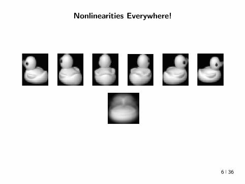
Nonlinearities Everywhere
Large l =rArr Big models H ldquorichrdquo non-parametricnonlinear
6 36
Nonlinearities Everywhere
Large l =rArr Big models H ldquorichrdquo non-parametricnonlinear
6 36
Choice of Nonlinear Hypothesis Space Kernels
x Ψ wTΨ(x) y
w
Ψ(x)
I eg Linear functions and Polynomials
I Infinite-dimensional nonlinear embeddings Fully non-parameteric
I Functional Analysis (Aronszajn Bergman (1950s)) Statistics (Parzen(1960s)) PDEs Numerical Analysis
I ML in 1990rsquos Nonlinear classification regression clustering time-seriesanalysis dynamical systems hypothesis testing causal modeling
I Convex Optimization
7 36
Choice of Nonlinear Hypothesis Space Deep Learning
x0 f1 f2 fL `
w1 w2 wL
z isin Rx1 x2 xLminus1 xL
I Compositions Raw data to higher abstractions (representation learning)
I Multilayer Perceptrons fl(xW) = σ(Wx) (sigmoids ReLU)I Turing (1950) In considering the functions of the mind or the brain we find certain operations which we can explain in
purely mechanical terms This we say does not correspond to the real mind it is a sort of skin which we must strip off if we are
to find the real mind Proceeding in this way do we ever come to the rdquorealrdquo mind or do we eventually come to the skin which
has nothing in it In the latter case the whole mind is mechanical
I Rosenblatt (1957) NYT 1958 New Navy Device Learns By Doing The Navy revealed the embryo of an electronic
computer today that it expects will be able to walk talk see write reproduce itself and be conscious of its existence Later
perceptrons will be able to recognize people and call out their names and instantly translate speech in one language to speech
and writing in another language it was predicted
I Perceptron (Minski and Pappert 1969) [Olarzan A Sociological Study 1996]I Backprop (1986) Reverse-mode differentiation (1960s-70s) CNNs (1980s 2012-)I Breadth-Width tradeoffsI Non-convex Optimization Domain-agnostic recipe
8 36
Choice of Nonlinear Hypothesis Space Deep Learning
x0 f1 f2 fL `
w1 w2 wL
z isin Rx1 x2 xLminus1 xL
I Compositions Raw data to higher abstractions (representation learning)I Multilayer Perceptrons fl(xW) = σ(Wx) (sigmoids ReLU)
I Turing (1950) In considering the functions of the mind or the brain we find certain operations which we can explain in
purely mechanical terms This we say does not correspond to the real mind it is a sort of skin which we must strip off if we are
to find the real mind Proceeding in this way do we ever come to the rdquorealrdquo mind or do we eventually come to the skin which
has nothing in it In the latter case the whole mind is mechanical
I Rosenblatt (1957) NYT 1958 New Navy Device Learns By Doing The Navy revealed the embryo of an electronic
computer today that it expects will be able to walk talk see write reproduce itself and be conscious of its existence Later
perceptrons will be able to recognize people and call out their names and instantly translate speech in one language to speech
and writing in another language it was predicted
I Perceptron (Minski and Pappert 1969) [Olarzan A Sociological Study 1996]I Backprop (1986) Reverse-mode differentiation (1960s-70s) CNNs (1980s 2012-)I Breadth-Width tradeoffsI Non-convex Optimization Domain-agnostic recipe
8 36
Choice of Nonlinear Hypothesis Space Deep Learning
x0 f1 f2 fL `
w1 w2 wL
z isin Rx1 x2 xLminus1 xL
I Compositions Raw data to higher abstractions (representation learning)I Multilayer Perceptrons fl(xW) = σ(Wx) (sigmoids ReLU)I Turing (1950) In considering the functions of the mind or the brain we find certain operations which we can explain in
purely mechanical terms This we say does not correspond to the real mind it is a sort of skin which we must strip off if we are
to find the real mind Proceeding in this way do we ever come to the rdquorealrdquo mind or do we eventually come to the skin which
has nothing in it In the latter case the whole mind is mechanical
I Rosenblatt (1957) NYT 1958 New Navy Device Learns By Doing The Navy revealed the embryo of an electronic
computer today that it expects will be able to walk talk see write reproduce itself and be conscious of its existence Later
perceptrons will be able to recognize people and call out their names and instantly translate speech in one language to speech
and writing in another language it was predicted
I Perceptron (Minski and Pappert 1969) [Olarzan A Sociological Study 1996]I Backprop (1986) Reverse-mode differentiation (1960s-70s) CNNs (1980s 2012-)I Breadth-Width tradeoffsI Non-convex Optimization Domain-agnostic recipe
8 36
Choice of Nonlinear Hypothesis Space Deep Learning
x0 f1 f2 fL `
w1 w2 wL
z isin Rx1 x2 xLminus1 xL
I Compositions Raw data to higher abstractions (representation learning)I Multilayer Perceptrons fl(xW) = σ(Wx) (sigmoids ReLU)I Turing (1950) In considering the functions of the mind or the brain we find certain operations which we can explain in
purely mechanical terms This we say does not correspond to the real mind it is a sort of skin which we must strip off if we are
to find the real mind Proceeding in this way do we ever come to the rdquorealrdquo mind or do we eventually come to the skin which
has nothing in it In the latter case the whole mind is mechanical
I Rosenblatt (1957) NYT 1958 New Navy Device Learns By Doing The Navy revealed the embryo of an electronic
computer today that it expects will be able to walk talk see write reproduce itself and be conscious of its existence Later
perceptrons will be able to recognize people and call out their names and instantly translate speech in one language to speech
and writing in another language it was predicted
I Perceptron (Minski and Pappert 1969) [Olarzan A Sociological Study 1996]I Backprop (1986) Reverse-mode differentiation (1960s-70s) CNNs (1980s 2012-)I Breadth-Width tradeoffsI Non-convex Optimization Domain-agnostic recipe
8 36
Choice of Nonlinear Hypothesis Space Deep Learning
x0 f1 f2 fL `
w1 w2 wL
z isin Rx1 x2 xLminus1 xL
I Compositions Raw data to higher abstractions (representation learning)I Multilayer Perceptrons fl(xW) = σ(Wx) (sigmoids ReLU)I Turing (1950) In considering the functions of the mind or the brain we find certain operations which we can explain in
purely mechanical terms This we say does not correspond to the real mind it is a sort of skin which we must strip off if we are
to find the real mind Proceeding in this way do we ever come to the rdquorealrdquo mind or do we eventually come to the skin which
has nothing in it In the latter case the whole mind is mechanical
I Rosenblatt (1957) NYT 1958 New Navy Device Learns By Doing The Navy revealed the embryo of an electronic
computer today that it expects will be able to walk talk see write reproduce itself and be conscious of its existence Later
perceptrons will be able to recognize people and call out their names and instantly translate speech in one language to speech
and writing in another language it was predicted
I Perceptron (Minski and Pappert 1969) [Olarzan A Sociological Study 1996]I Backprop (1986) Reverse-mode differentiation (1960s-70s) CNNs (1980s 2012-)
I Breadth-Width tradeoffsI Non-convex Optimization Domain-agnostic recipe
8 36
Choice of Nonlinear Hypothesis Space Deep Learning
x0 f1 f2 fL `
w1 w2 wL
z isin Rx1 x2 xLminus1 xL
I Compositions Raw data to higher abstractions (representation learning)I Multilayer Perceptrons fl(xW) = σ(Wx) (sigmoids ReLU)I Turing (1950) In considering the functions of the mind or the brain we find certain operations which we can explain in
purely mechanical terms This we say does not correspond to the real mind it is a sort of skin which we must strip off if we are
to find the real mind Proceeding in this way do we ever come to the rdquorealrdquo mind or do we eventually come to the skin which
has nothing in it In the latter case the whole mind is mechanical
I Rosenblatt (1957) NYT 1958 New Navy Device Learns By Doing The Navy revealed the embryo of an electronic
computer today that it expects will be able to walk talk see write reproduce itself and be conscious of its existence Later
perceptrons will be able to recognize people and call out their names and instantly translate speech in one language to speech
and writing in another language it was predicted
I Perceptron (Minski and Pappert 1969) [Olarzan A Sociological Study 1996]I Backprop (1986) Reverse-mode differentiation (1960s-70s) CNNs (1980s 2012-)I Breadth-Width tradeoffsI Non-convex Optimization Domain-agnostic recipe 8 36
Choice of Nonlinear Hypothesis Space Deep Learning
x0 f1 f2 fL `
w1 w2 wL
z isin Rx1 x2 xLminus1 xL
I Compositions Raw data to higher abstractions (representation learning)I Multilayer Perceptrons fl(xW) = σ(Wx) (sigmoids ReLU)I Turing (1950) In considering the functions of the mind or the brain we find certain operations which we can explain in
purely mechanical terms This we say does not correspond to the real mind it is a sort of skin which we must strip off if we are
to find the real mind Proceeding in this way do we ever come to the rdquorealrdquo mind or do we eventually come to the skin which
has nothing in it In the latter case the whole mind is mechanical
I Rosenblatt (1957) NYT 1958 New Navy Device Learns By Doing The Navy revealed the embryo of an electronic
computer today that it expects will be able to walk talk see write reproduce itself and be conscious of its existence Later
perceptrons will be able to recognize people and call out their names and instantly translate speech in one language to speech
and writing in another language it was predicted
I Perceptron (Minski and Pappert 1969) [Olarzan A Sociological Study 1996]I Backprop (1986) Reverse-mode differentiation (1960s-70s) CNNs (1980s 2012-)I Breadth-Width tradeoffsI Non-convex Optimization Domain-agnostic recipe 8 36
The Watershed Moment Imagenet 2012
I Many statistical and computational ingredientsndash Large datasets (ILSVRC since 2010)
ndash Large statistical capacity (12M images 60M params)ndash Distributed computationndash Depth Invariant feature learning (transferrable to other tasks)ndash Engineering Dropout ReLU
I Many astonishing results since then
9 36
The Watershed Moment Imagenet 2012
I Many statistical and computational ingredientsndash Large datasets (ILSVRC since 2010)ndash Large statistical capacity (12M images 60M params)
ndash Distributed computationndash Depth Invariant feature learning (transferrable to other tasks)ndash Engineering Dropout ReLU
I Many astonishing results since then
9 36
The Watershed Moment Imagenet 2012
I Many statistical and computational ingredientsndash Large datasets (ILSVRC since 2010)ndash Large statistical capacity (12M images 60M params)ndash Distributed computation
ndash Depth Invariant feature learning (transferrable to other tasks)ndash Engineering Dropout ReLU
I Many astonishing results since then
9 36
The Watershed Moment Imagenet 2012
I Many statistical and computational ingredientsndash Large datasets (ILSVRC since 2010)ndash Large statistical capacity (12M images 60M params)ndash Distributed computationndash Depth Invariant feature learning (transferrable to other tasks)
ndash Engineering Dropout ReLU I Many astonishing results since then
9 36
The Watershed Moment Imagenet 2012
I Many statistical and computational ingredientsndash Large datasets (ILSVRC since 2010)ndash Large statistical capacity (12M images 60M params)ndash Distributed computationndash Depth Invariant feature learning (transferrable to other tasks)ndash Engineering Dropout ReLU
I Many astonishing results since then
9 36
CNNs
10 36
Self-Driving Cars
Figure End-to-End Learning for Self-driving Cars Bojarski et al 2016
11 36

Nonlinearities Everywhere
Large l =rArr Big models H ldquorichrdquo non-parametricnonlinear
6 36
Choice of Nonlinear Hypothesis Space Kernels
x Ψ wTΨ(x) y
w
Ψ(x)
I eg Linear functions and Polynomials
I Infinite-dimensional nonlinear embeddings Fully non-parameteric
I Functional Analysis (Aronszajn Bergman (1950s)) Statistics (Parzen(1960s)) PDEs Numerical Analysis
I ML in 1990rsquos Nonlinear classification regression clustering time-seriesanalysis dynamical systems hypothesis testing causal modeling
I Convex Optimization
7 36
Choice of Nonlinear Hypothesis Space Deep Learning
x0 f1 f2 fL `
w1 w2 wL
z isin Rx1 x2 xLminus1 xL
I Compositions Raw data to higher abstractions (representation learning)
I Multilayer Perceptrons fl(xW) = σ(Wx) (sigmoids ReLU)I Turing (1950) In considering the functions of the mind or the brain we find certain operations which we can explain in
purely mechanical terms This we say does not correspond to the real mind it is a sort of skin which we must strip off if we are
to find the real mind Proceeding in this way do we ever come to the rdquorealrdquo mind or do we eventually come to the skin which
has nothing in it In the latter case the whole mind is mechanical
I Rosenblatt (1957) NYT 1958 New Navy Device Learns By Doing The Navy revealed the embryo of an electronic
computer today that it expects will be able to walk talk see write reproduce itself and be conscious of its existence Later
perceptrons will be able to recognize people and call out their names and instantly translate speech in one language to speech
and writing in another language it was predicted
I Perceptron (Minski and Pappert 1969) [Olarzan A Sociological Study 1996]I Backprop (1986) Reverse-mode differentiation (1960s-70s) CNNs (1980s 2012-)I Breadth-Width tradeoffsI Non-convex Optimization Domain-agnostic recipe
8 36
Choice of Nonlinear Hypothesis Space Deep Learning
x0 f1 f2 fL `
w1 w2 wL
z isin Rx1 x2 xLminus1 xL
I Compositions Raw data to higher abstractions (representation learning)I Multilayer Perceptrons fl(xW) = σ(Wx) (sigmoids ReLU)
I Turing (1950) In considering the functions of the mind or the brain we find certain operations which we can explain in
purely mechanical terms This we say does not correspond to the real mind it is a sort of skin which we must strip off if we are
to find the real mind Proceeding in this way do we ever come to the rdquorealrdquo mind or do we eventually come to the skin which
has nothing in it In the latter case the whole mind is mechanical
I Rosenblatt (1957) NYT 1958 New Navy Device Learns By Doing The Navy revealed the embryo of an electronic
computer today that it expects will be able to walk talk see write reproduce itself and be conscious of its existence Later
perceptrons will be able to recognize people and call out their names and instantly translate speech in one language to speech
and writing in another language it was predicted
I Perceptron (Minski and Pappert 1969) [Olarzan A Sociological Study 1996]I Backprop (1986) Reverse-mode differentiation (1960s-70s) CNNs (1980s 2012-)I Breadth-Width tradeoffsI Non-convex Optimization Domain-agnostic recipe
8 36
Choice of Nonlinear Hypothesis Space Deep Learning
x0 f1 f2 fL `
w1 w2 wL
z isin Rx1 x2 xLminus1 xL
I Compositions Raw data to higher abstractions (representation learning)I Multilayer Perceptrons fl(xW) = σ(Wx) (sigmoids ReLU)I Turing (1950) In considering the functions of the mind or the brain we find certain operations which we can explain in
purely mechanical terms This we say does not correspond to the real mind it is a sort of skin which we must strip off if we are
to find the real mind Proceeding in this way do we ever come to the rdquorealrdquo mind or do we eventually come to the skin which
has nothing in it In the latter case the whole mind is mechanical
I Rosenblatt (1957) NYT 1958 New Navy Device Learns By Doing The Navy revealed the embryo of an electronic
computer today that it expects will be able to walk talk see write reproduce itself and be conscious of its existence Later
perceptrons will be able to recognize people and call out their names and instantly translate speech in one language to speech
and writing in another language it was predicted
I Perceptron (Minski and Pappert 1969) [Olarzan A Sociological Study 1996]I Backprop (1986) Reverse-mode differentiation (1960s-70s) CNNs (1980s 2012-)I Breadth-Width tradeoffsI Non-convex Optimization Domain-agnostic recipe
8 36
Choice of Nonlinear Hypothesis Space Deep Learning
x0 f1 f2 fL `
w1 w2 wL
z isin Rx1 x2 xLminus1 xL
I Compositions Raw data to higher abstractions (representation learning)I Multilayer Perceptrons fl(xW) = σ(Wx) (sigmoids ReLU)I Turing (1950) In considering the functions of the mind or the brain we find certain operations which we can explain in
purely mechanical terms This we say does not correspond to the real mind it is a sort of skin which we must strip off if we are
to find the real mind Proceeding in this way do we ever come to the rdquorealrdquo mind or do we eventually come to the skin which
has nothing in it In the latter case the whole mind is mechanical
I Rosenblatt (1957) NYT 1958 New Navy Device Learns By Doing The Navy revealed the embryo of an electronic
computer today that it expects will be able to walk talk see write reproduce itself and be conscious of its existence Later
perceptrons will be able to recognize people and call out their names and instantly translate speech in one language to speech
and writing in another language it was predicted
I Perceptron (Minski and Pappert 1969) [Olarzan A Sociological Study 1996]I Backprop (1986) Reverse-mode differentiation (1960s-70s) CNNs (1980s 2012-)I Breadth-Width tradeoffsI Non-convex Optimization Domain-agnostic recipe
8 36
Choice of Nonlinear Hypothesis Space Deep Learning
x0 f1 f2 fL `
w1 w2 wL
z isin Rx1 x2 xLminus1 xL
I Compositions Raw data to higher abstractions (representation learning)I Multilayer Perceptrons fl(xW) = σ(Wx) (sigmoids ReLU)I Turing (1950) In considering the functions of the mind or the brain we find certain operations which we can explain in
purely mechanical terms This we say does not correspond to the real mind it is a sort of skin which we must strip off if we are
to find the real mind Proceeding in this way do we ever come to the rdquorealrdquo mind or do we eventually come to the skin which
has nothing in it In the latter case the whole mind is mechanical
I Rosenblatt (1957) NYT 1958 New Navy Device Learns By Doing The Navy revealed the embryo of an electronic
computer today that it expects will be able to walk talk see write reproduce itself and be conscious of its existence Later
perceptrons will be able to recognize people and call out their names and instantly translate speech in one language to speech
and writing in another language it was predicted
I Perceptron (Minski and Pappert 1969) [Olarzan A Sociological Study 1996]I Backprop (1986) Reverse-mode differentiation (1960s-70s) CNNs (1980s 2012-)
I Breadth-Width tradeoffsI Non-convex Optimization Domain-agnostic recipe
8 36
Choice of Nonlinear Hypothesis Space Deep Learning
x0 f1 f2 fL `
w1 w2 wL
z isin Rx1 x2 xLminus1 xL
I Compositions Raw data to higher abstractions (representation learning)I Multilayer Perceptrons fl(xW) = σ(Wx) (sigmoids ReLU)I Turing (1950) In considering the functions of the mind or the brain we find certain operations which we can explain in
purely mechanical terms This we say does not correspond to the real mind it is a sort of skin which we must strip off if we are
to find the real mind Proceeding in this way do we ever come to the rdquorealrdquo mind or do we eventually come to the skin which
has nothing in it In the latter case the whole mind is mechanical
I Rosenblatt (1957) NYT 1958 New Navy Device Learns By Doing The Navy revealed the embryo of an electronic
computer today that it expects will be able to walk talk see write reproduce itself and be conscious of its existence Later
perceptrons will be able to recognize people and call out their names and instantly translate speech in one language to speech
and writing in another language it was predicted
I Perceptron (Minski and Pappert 1969) [Olarzan A Sociological Study 1996]I Backprop (1986) Reverse-mode differentiation (1960s-70s) CNNs (1980s 2012-)I Breadth-Width tradeoffsI Non-convex Optimization Domain-agnostic recipe 8 36
Choice of Nonlinear Hypothesis Space Deep Learning
x0 f1 f2 fL `
w1 w2 wL
z isin Rx1 x2 xLminus1 xL
I Compositions Raw data to higher abstractions (representation learning)I Multilayer Perceptrons fl(xW) = σ(Wx) (sigmoids ReLU)I Turing (1950) In considering the functions of the mind or the brain we find certain operations which we can explain in
purely mechanical terms This we say does not correspond to the real mind it is a sort of skin which we must strip off if we are
to find the real mind Proceeding in this way do we ever come to the rdquorealrdquo mind or do we eventually come to the skin which
has nothing in it In the latter case the whole mind is mechanical
I Rosenblatt (1957) NYT 1958 New Navy Device Learns By Doing The Navy revealed the embryo of an electronic
computer today that it expects will be able to walk talk see write reproduce itself and be conscious of its existence Later
perceptrons will be able to recognize people and call out their names and instantly translate speech in one language to speech
and writing in another language it was predicted
I Perceptron (Minski and Pappert 1969) [Olarzan A Sociological Study 1996]I Backprop (1986) Reverse-mode differentiation (1960s-70s) CNNs (1980s 2012-)I Breadth-Width tradeoffsI Non-convex Optimization Domain-agnostic recipe 8 36
The Watershed Moment Imagenet 2012
I Many statistical and computational ingredientsndash Large datasets (ILSVRC since 2010)
ndash Large statistical capacity (12M images 60M params)ndash Distributed computationndash Depth Invariant feature learning (transferrable to other tasks)ndash Engineering Dropout ReLU
I Many astonishing results since then
9 36
The Watershed Moment Imagenet 2012
I Many statistical and computational ingredientsndash Large datasets (ILSVRC since 2010)ndash Large statistical capacity (12M images 60M params)
ndash Distributed computationndash Depth Invariant feature learning (transferrable to other tasks)ndash Engineering Dropout ReLU
I Many astonishing results since then
9 36
The Watershed Moment Imagenet 2012
I Many statistical and computational ingredientsndash Large datasets (ILSVRC since 2010)ndash Large statistical capacity (12M images 60M params)ndash Distributed computation
ndash Depth Invariant feature learning (transferrable to other tasks)ndash Engineering Dropout ReLU
I Many astonishing results since then
9 36
The Watershed Moment Imagenet 2012
I Many statistical and computational ingredientsndash Large datasets (ILSVRC since 2010)ndash Large statistical capacity (12M images 60M params)ndash Distributed computationndash Depth Invariant feature learning (transferrable to other tasks)
ndash Engineering Dropout ReLU I Many astonishing results since then
9 36
The Watershed Moment Imagenet 2012
I Many statistical and computational ingredientsndash Large datasets (ILSVRC since 2010)ndash Large statistical capacity (12M images 60M params)ndash Distributed computationndash Depth Invariant feature learning (transferrable to other tasks)ndash Engineering Dropout ReLU
I Many astonishing results since then
9 36
CNNs
10 36
Self-Driving Cars
Figure End-to-End Learning for Self-driving Cars Bojarski et al 2016
11 36

Choice of Nonlinear Hypothesis Space Kernels
x Ψ wTΨ(x) y
w
Ψ(x)
I eg Linear functions and Polynomials
I Infinite-dimensional nonlinear embeddings Fully non-parameteric
I Functional Analysis (Aronszajn Bergman (1950s)) Statistics (Parzen(1960s)) PDEs Numerical Analysis
I ML in 1990rsquos Nonlinear classification regression clustering time-seriesanalysis dynamical systems hypothesis testing causal modeling
I Convex Optimization
7 36
Choice of Nonlinear Hypothesis Space Deep Learning
x0 f1 f2 fL `
w1 w2 wL
z isin Rx1 x2 xLminus1 xL
I Compositions Raw data to higher abstractions (representation learning)
I Multilayer Perceptrons fl(xW) = σ(Wx) (sigmoids ReLU)I Turing (1950) In considering the functions of the mind or the brain we find certain operations which we can explain in
purely mechanical terms This we say does not correspond to the real mind it is a sort of skin which we must strip off if we are
to find the real mind Proceeding in this way do we ever come to the rdquorealrdquo mind or do we eventually come to the skin which
has nothing in it In the latter case the whole mind is mechanical
I Rosenblatt (1957) NYT 1958 New Navy Device Learns By Doing The Navy revealed the embryo of an electronic
computer today that it expects will be able to walk talk see write reproduce itself and be conscious of its existence Later
perceptrons will be able to recognize people and call out their names and instantly translate speech in one language to speech
and writing in another language it was predicted
I Perceptron (Minski and Pappert 1969) [Olarzan A Sociological Study 1996]I Backprop (1986) Reverse-mode differentiation (1960s-70s) CNNs (1980s 2012-)I Breadth-Width tradeoffsI Non-convex Optimization Domain-agnostic recipe
8 36
Choice of Nonlinear Hypothesis Space Deep Learning
x0 f1 f2 fL `
w1 w2 wL
z isin Rx1 x2 xLminus1 xL
I Compositions Raw data to higher abstractions (representation learning)I Multilayer Perceptrons fl(xW) = σ(Wx) (sigmoids ReLU)
I Turing (1950) In considering the functions of the mind or the brain we find certain operations which we can explain in
purely mechanical terms This we say does not correspond to the real mind it is a sort of skin which we must strip off if we are
to find the real mind Proceeding in this way do we ever come to the rdquorealrdquo mind or do we eventually come to the skin which
has nothing in it In the latter case the whole mind is mechanical
I Rosenblatt (1957) NYT 1958 New Navy Device Learns By Doing The Navy revealed the embryo of an electronic
computer today that it expects will be able to walk talk see write reproduce itself and be conscious of its existence Later
perceptrons will be able to recognize people and call out their names and instantly translate speech in one language to speech
and writing in another language it was predicted
I Perceptron (Minski and Pappert 1969) [Olarzan A Sociological Study 1996]I Backprop (1986) Reverse-mode differentiation (1960s-70s) CNNs (1980s 2012-)I Breadth-Width tradeoffsI Non-convex Optimization Domain-agnostic recipe
8 36
Choice of Nonlinear Hypothesis Space Deep Learning
x0 f1 f2 fL `
w1 w2 wL
z isin Rx1 x2 xLminus1 xL
I Compositions Raw data to higher abstractions (representation learning)I Multilayer Perceptrons fl(xW) = σ(Wx) (sigmoids ReLU)I Turing (1950) In considering the functions of the mind or the brain we find certain operations which we can explain in
purely mechanical terms This we say does not correspond to the real mind it is a sort of skin which we must strip off if we are
to find the real mind Proceeding in this way do we ever come to the rdquorealrdquo mind or do we eventually come to the skin which
has nothing in it In the latter case the whole mind is mechanical
I Rosenblatt (1957) NYT 1958 New Navy Device Learns By Doing The Navy revealed the embryo of an electronic
computer today that it expects will be able to walk talk see write reproduce itself and be conscious of its existence Later
perceptrons will be able to recognize people and call out their names and instantly translate speech in one language to speech
and writing in another language it was predicted
I Perceptron (Minski and Pappert 1969) [Olarzan A Sociological Study 1996]I Backprop (1986) Reverse-mode differentiation (1960s-70s) CNNs (1980s 2012-)I Breadth-Width tradeoffsI Non-convex Optimization Domain-agnostic recipe
8 36
Choice of Nonlinear Hypothesis Space Deep Learning
x0 f1 f2 fL `
w1 w2 wL
z isin Rx1 x2 xLminus1 xL
I Compositions Raw data to higher abstractions (representation learning)I Multilayer Perceptrons fl(xW) = σ(Wx) (sigmoids ReLU)I Turing (1950) In considering the functions of the mind or the brain we find certain operations which we can explain in
purely mechanical terms This we say does not correspond to the real mind it is a sort of skin which we must strip off if we are
to find the real mind Proceeding in this way do we ever come to the rdquorealrdquo mind or do we eventually come to the skin which
has nothing in it In the latter case the whole mind is mechanical
I Rosenblatt (1957) NYT 1958 New Navy Device Learns By Doing The Navy revealed the embryo of an electronic
computer today that it expects will be able to walk talk see write reproduce itself and be conscious of its existence Later
perceptrons will be able to recognize people and call out their names and instantly translate speech in one language to speech
and writing in another language it was predicted
I Perceptron (Minski and Pappert 1969) [Olarzan A Sociological Study 1996]I Backprop (1986) Reverse-mode differentiation (1960s-70s) CNNs (1980s 2012-)I Breadth-Width tradeoffsI Non-convex Optimization Domain-agnostic recipe
8 36
Choice of Nonlinear Hypothesis Space Deep Learning
x0 f1 f2 fL `
w1 w2 wL
z isin Rx1 x2 xLminus1 xL
I Compositions Raw data to higher abstractions (representation learning)I Multilayer Perceptrons fl(xW) = σ(Wx) (sigmoids ReLU)I Turing (1950) In considering the functions of the mind or the brain we find certain operations which we can explain in
purely mechanical terms This we say does not correspond to the real mind it is a sort of skin which we must strip off if we are
to find the real mind Proceeding in this way do we ever come to the rdquorealrdquo mind or do we eventually come to the skin which
has nothing in it In the latter case the whole mind is mechanical
I Rosenblatt (1957) NYT 1958 New Navy Device Learns By Doing The Navy revealed the embryo of an electronic
computer today that it expects will be able to walk talk see write reproduce itself and be conscious of its existence Later
perceptrons will be able to recognize people and call out their names and instantly translate speech in one language to speech
and writing in another language it was predicted
I Perceptron (Minski and Pappert 1969) [Olarzan A Sociological Study 1996]I Backprop (1986) Reverse-mode differentiation (1960s-70s) CNNs (1980s 2012-)
I Breadth-Width tradeoffsI Non-convex Optimization Domain-agnostic recipe
8 36
Choice of Nonlinear Hypothesis Space Deep Learning
x0 f1 f2 fL `
w1 w2 wL
z isin Rx1 x2 xLminus1 xL
I Compositions Raw data to higher abstractions (representation learning)I Multilayer Perceptrons fl(xW) = σ(Wx) (sigmoids ReLU)I Turing (1950) In considering the functions of the mind or the brain we find certain operations which we can explain in
purely mechanical terms This we say does not correspond to the real mind it is a sort of skin which we must strip off if we are
to find the real mind Proceeding in this way do we ever come to the rdquorealrdquo mind or do we eventually come to the skin which
has nothing in it In the latter case the whole mind is mechanical
I Rosenblatt (1957) NYT 1958 New Navy Device Learns By Doing The Navy revealed the embryo of an electronic
computer today that it expects will be able to walk talk see write reproduce itself and be conscious of its existence Later
perceptrons will be able to recognize people and call out their names and instantly translate speech in one language to speech
and writing in another language it was predicted
I Perceptron (Minski and Pappert 1969) [Olarzan A Sociological Study 1996]I Backprop (1986) Reverse-mode differentiation (1960s-70s) CNNs (1980s 2012-)I Breadth-Width tradeoffsI Non-convex Optimization Domain-agnostic recipe 8 36
Choice of Nonlinear Hypothesis Space Deep Learning
x0 f1 f2 fL `
w1 w2 wL
z isin Rx1 x2 xLminus1 xL
I Compositions Raw data to higher abstractions (representation learning)I Multilayer Perceptrons fl(xW) = σ(Wx) (sigmoids ReLU)I Turing (1950) In considering the functions of the mind or the brain we find certain operations which we can explain in
purely mechanical terms This we say does not correspond to the real mind it is a sort of skin which we must strip off if we are
to find the real mind Proceeding in this way do we ever come to the rdquorealrdquo mind or do we eventually come to the skin which
has nothing in it In the latter case the whole mind is mechanical
I Rosenblatt (1957) NYT 1958 New Navy Device Learns By Doing The Navy revealed the embryo of an electronic
computer today that it expects will be able to walk talk see write reproduce itself and be conscious of its existence Later
perceptrons will be able to recognize people and call out their names and instantly translate speech in one language to speech
and writing in another language it was predicted
I Perceptron (Minski and Pappert 1969) [Olarzan A Sociological Study 1996]I Backprop (1986) Reverse-mode differentiation (1960s-70s) CNNs (1980s 2012-)I Breadth-Width tradeoffsI Non-convex Optimization Domain-agnostic recipe 8 36
The Watershed Moment Imagenet 2012
I Many statistical and computational ingredientsndash Large datasets (ILSVRC since 2010)
ndash Large statistical capacity (12M images 60M params)ndash Distributed computationndash Depth Invariant feature learning (transferrable to other tasks)ndash Engineering Dropout ReLU
I Many astonishing results since then
9 36
The Watershed Moment Imagenet 2012
I Many statistical and computational ingredientsndash Large datasets (ILSVRC since 2010)ndash Large statistical capacity (12M images 60M params)
ndash Distributed computationndash Depth Invariant feature learning (transferrable to other tasks)ndash Engineering Dropout ReLU
I Many astonishing results since then
9 36
The Watershed Moment Imagenet 2012
I Many statistical and computational ingredientsndash Large datasets (ILSVRC since 2010)ndash Large statistical capacity (12M images 60M params)ndash Distributed computation
ndash Depth Invariant feature learning (transferrable to other tasks)ndash Engineering Dropout ReLU
I Many astonishing results since then
9 36
The Watershed Moment Imagenet 2012
I Many statistical and computational ingredientsndash Large datasets (ILSVRC since 2010)ndash Large statistical capacity (12M images 60M params)ndash Distributed computationndash Depth Invariant feature learning (transferrable to other tasks)
ndash Engineering Dropout ReLU I Many astonishing results since then
9 36
The Watershed Moment Imagenet 2012
I Many statistical and computational ingredientsndash Large datasets (ILSVRC since 2010)ndash Large statistical capacity (12M images 60M params)ndash Distributed computationndash Depth Invariant feature learning (transferrable to other tasks)ndash Engineering Dropout ReLU
I Many astonishing results since then
9 36
CNNs
10 36
Self-Driving Cars
Figure End-to-End Learning for Self-driving Cars Bojarski et al 2016
11 36

Choice of Nonlinear Hypothesis Space Kernels
x Ψ wTΨ(x) y
w
Ψ(x)
I eg Linear functions and Polynomials
I Infinite-dimensional nonlinear embeddings Fully non-parameteric
I Functional Analysis (Aronszajn Bergman (1950s)) Statistics (Parzen(1960s)) PDEs Numerical Analysis
I ML in 1990rsquos Nonlinear classification regression clustering time-seriesanalysis dynamical systems hypothesis testing causal modeling
I Convex Optimization
7 36
Choice of Nonlinear Hypothesis Space Kernels
x Ψ wTΨ(x) y
w
Ψ(x)
I eg Linear functions and Polynomials
I Infinite-dimensional nonlinear embeddings Fully non-parameteric
I Functional Analysis (Aronszajn Bergman (1950s)) Statistics (Parzen(1960s)) PDEs Numerical Analysis
I ML in 1990rsquos Nonlinear classification regression clustering time-seriesanalysis dynamical systems hypothesis testing causal modeling
I Convex Optimization
7 36
Choice of Nonlinear Hypothesis Space Kernels
x Ψ wTΨ(x) y
w
Ψ(x)
I eg Linear functions and Polynomials
I Infinite-dimensional nonlinear embeddings Fully non-parameteric
I Functional Analysis (Aronszajn Bergman (1950s)) Statistics (Parzen(1960s)) PDEs Numerical Analysis
I ML in 1990rsquos Nonlinear classification regression clustering time-seriesanalysis dynamical systems hypothesis testing causal modeling
I Convex Optimization
7 36
Choice of Nonlinear Hypothesis Space Kernels
x Ψ wTΨ(x) y
w
Ψ(x)
I eg Linear functions and Polynomials
I Infinite-dimensional nonlinear embeddings Fully non-parameteric
I Functional Analysis (Aronszajn Bergman (1950s)) Statistics (Parzen(1960s)) PDEs Numerical Analysis
I ML in 1990rsquos Nonlinear classification regression clustering time-seriesanalysis dynamical systems hypothesis testing causal modeling
I Convex Optimization
7 36
Choice of Nonlinear Hypothesis Space Deep Learning
x0 f1 f2 fL `
w1 w2 wL
z isin Rx1 x2 xLminus1 xL
I Compositions Raw data to higher abstractions (representation learning)
I Multilayer Perceptrons fl(xW) = σ(Wx) (sigmoids ReLU)I Turing (1950) In considering the functions of the mind or the brain we find certain operations which we can explain in
purely mechanical terms This we say does not correspond to the real mind it is a sort of skin which we must strip off if we are
to find the real mind Proceeding in this way do we ever come to the rdquorealrdquo mind or do we eventually come to the skin which
has nothing in it In the latter case the whole mind is mechanical
I Rosenblatt (1957) NYT 1958 New Navy Device Learns By Doing The Navy revealed the embryo of an electronic
computer today that it expects will be able to walk talk see write reproduce itself and be conscious of its existence Later
perceptrons will be able to recognize people and call out their names and instantly translate speech in one language to speech
and writing in another language it was predicted
I Perceptron (Minski and Pappert 1969) [Olarzan A Sociological Study 1996]I Backprop (1986) Reverse-mode differentiation (1960s-70s) CNNs (1980s 2012-)I Breadth-Width tradeoffsI Non-convex Optimization Domain-agnostic recipe
8 36
Choice of Nonlinear Hypothesis Space Deep Learning
x0 f1 f2 fL `
w1 w2 wL
z isin Rx1 x2 xLminus1 xL
I Compositions Raw data to higher abstractions (representation learning)I Multilayer Perceptrons fl(xW) = σ(Wx) (sigmoids ReLU)
I Turing (1950) In considering the functions of the mind or the brain we find certain operations which we can explain in
purely mechanical terms This we say does not correspond to the real mind it is a sort of skin which we must strip off if we are
to find the real mind Proceeding in this way do we ever come to the rdquorealrdquo mind or do we eventually come to the skin which
has nothing in it In the latter case the whole mind is mechanical
I Rosenblatt (1957) NYT 1958 New Navy Device Learns By Doing The Navy revealed the embryo of an electronic
computer today that it expects will be able to walk talk see write reproduce itself and be conscious of its existence Later
perceptrons will be able to recognize people and call out their names and instantly translate speech in one language to speech
and writing in another language it was predicted
I Perceptron (Minski and Pappert 1969) [Olarzan A Sociological Study 1996]I Backprop (1986) Reverse-mode differentiation (1960s-70s) CNNs (1980s 2012-)I Breadth-Width tradeoffsI Non-convex Optimization Domain-agnostic recipe
8 36
Choice of Nonlinear Hypothesis Space Deep Learning
x0 f1 f2 fL `
w1 w2 wL
z isin Rx1 x2 xLminus1 xL
I Compositions Raw data to higher abstractions (representation learning)I Multilayer Perceptrons fl(xW) = σ(Wx) (sigmoids ReLU)I Turing (1950) In considering the functions of the mind or the brain we find certain operations which we can explain in
purely mechanical terms This we say does not correspond to the real mind it is a sort of skin which we must strip off if we are
to find the real mind Proceeding in this way do we ever come to the rdquorealrdquo mind or do we eventually come to the skin which
has nothing in it In the latter case the whole mind is mechanical
I Rosenblatt (1957) NYT 1958 New Navy Device Learns By Doing The Navy revealed the embryo of an electronic
computer today that it expects will be able to walk talk see write reproduce itself and be conscious of its existence Later
perceptrons will be able to recognize people and call out their names and instantly translate speech in one language to speech
and writing in another language it was predicted
I Perceptron (Minski and Pappert 1969) [Olarzan A Sociological Study 1996]I Backprop (1986) Reverse-mode differentiation (1960s-70s) CNNs (1980s 2012-)I Breadth-Width tradeoffsI Non-convex Optimization Domain-agnostic recipe
8 36
Choice of Nonlinear Hypothesis Space Deep Learning
x0 f1 f2 fL `
w1 w2 wL
z isin Rx1 x2 xLminus1 xL
I Compositions Raw data to higher abstractions (representation learning)I Multilayer Perceptrons fl(xW) = σ(Wx) (sigmoids ReLU)I Turing (1950) In considering the functions of the mind or the brain we find certain operations which we can explain in
purely mechanical terms This we say does not correspond to the real mind it is a sort of skin which we must strip off if we are
to find the real mind Proceeding in this way do we ever come to the rdquorealrdquo mind or do we eventually come to the skin which
has nothing in it In the latter case the whole mind is mechanical
I Rosenblatt (1957) NYT 1958 New Navy Device Learns By Doing The Navy revealed the embryo of an electronic
computer today that it expects will be able to walk talk see write reproduce itself and be conscious of its existence Later
perceptrons will be able to recognize people and call out their names and instantly translate speech in one language to speech
and writing in another language it was predicted
I Perceptron (Minski and Pappert 1969) [Olarzan A Sociological Study 1996]I Backprop (1986) Reverse-mode differentiation (1960s-70s) CNNs (1980s 2012-)I Breadth-Width tradeoffsI Non-convex Optimization Domain-agnostic recipe
8 36
Choice of Nonlinear Hypothesis Space Deep Learning
x0 f1 f2 fL `
w1 w2 wL
z isin Rx1 x2 xLminus1 xL
I Compositions Raw data to higher abstractions (representation learning)I Multilayer Perceptrons fl(xW) = σ(Wx) (sigmoids ReLU)I Turing (1950) In considering the functions of the mind or the brain we find certain operations which we can explain in
purely mechanical terms This we say does not correspond to the real mind it is a sort of skin which we must strip off if we are
to find the real mind Proceeding in this way do we ever come to the rdquorealrdquo mind or do we eventually come to the skin which
has nothing in it In the latter case the whole mind is mechanical
I Rosenblatt (1957) NYT 1958 New Navy Device Learns By Doing The Navy revealed the embryo of an electronic
computer today that it expects will be able to walk talk see write reproduce itself and be conscious of its existence Later
perceptrons will be able to recognize people and call out their names and instantly translate speech in one language to speech
and writing in another language it was predicted
I Perceptron (Minski and Pappert 1969) [Olarzan A Sociological Study 1996]I Backprop (1986) Reverse-mode differentiation (1960s-70s) CNNs (1980s 2012-)
I Breadth-Width tradeoffsI Non-convex Optimization Domain-agnostic recipe
8 36
Choice of Nonlinear Hypothesis Space Deep Learning
x0 f1 f2 fL `
w1 w2 wL
z isin Rx1 x2 xLminus1 xL
I Compositions Raw data to higher abstractions (representation learning)I Multilayer Perceptrons fl(xW) = σ(Wx) (sigmoids ReLU)I Turing (1950) In considering the functions of the mind or the brain we find certain operations which we can explain in
purely mechanical terms This we say does not correspond to the real mind it is a sort of skin which we must strip off if we are
to find the real mind Proceeding in this way do we ever come to the rdquorealrdquo mind or do we eventually come to the skin which
has nothing in it In the latter case the whole mind is mechanical
I Rosenblatt (1957) NYT 1958 New Navy Device Learns By Doing The Navy revealed the embryo of an electronic
computer today that it expects will be able to walk talk see write reproduce itself and be conscious of its existence Later
perceptrons will be able to recognize people and call out their names and instantly translate speech in one language to speech
and writing in another language it was predicted
I Perceptron (Minski and Pappert 1969) [Olarzan A Sociological Study 1996]I Backprop (1986) Reverse-mode differentiation (1960s-70s) CNNs (1980s 2012-)I Breadth-Width tradeoffsI Non-convex Optimization Domain-agnostic recipe 8 36
Choice of Nonlinear Hypothesis Space Deep Learning
x0 f1 f2 fL `
w1 w2 wL
z isin Rx1 x2 xLminus1 xL
I Compositions Raw data to higher abstractions (representation learning)I Multilayer Perceptrons fl(xW) = σ(Wx) (sigmoids ReLU)I Turing (1950) In considering the functions of the mind or the brain we find certain operations which we can explain in
purely mechanical terms This we say does not correspond to the real mind it is a sort of skin which we must strip off if we are
to find the real mind Proceeding in this way do we ever come to the rdquorealrdquo mind or do we eventually come to the skin which
has nothing in it In the latter case the whole mind is mechanical
I Rosenblatt (1957) NYT 1958 New Navy Device Learns By Doing The Navy revealed the embryo of an electronic
computer today that it expects will be able to walk talk see write reproduce itself and be conscious of its existence Later
perceptrons will be able to recognize people and call out their names and instantly translate speech in one language to speech
and writing in another language it was predicted
I Perceptron (Minski and Pappert 1969) [Olarzan A Sociological Study 1996]I Backprop (1986) Reverse-mode differentiation (1960s-70s) CNNs (1980s 2012-)I Breadth-Width tradeoffsI Non-convex Optimization Domain-agnostic recipe 8 36
The Watershed Moment Imagenet 2012
I Many statistical and computational ingredientsndash Large datasets (ILSVRC since 2010)
ndash Large statistical capacity (12M images 60M params)ndash Distributed computationndash Depth Invariant feature learning (transferrable to other tasks)ndash Engineering Dropout ReLU
I Many astonishing results since then
9 36
The Watershed Moment Imagenet 2012
I Many statistical and computational ingredientsndash Large datasets (ILSVRC since 2010)ndash Large statistical capacity (12M images 60M params)
ndash Distributed computationndash Depth Invariant feature learning (transferrable to other tasks)ndash Engineering Dropout ReLU
I Many astonishing results since then
9 36
The Watershed Moment Imagenet 2012
I Many statistical and computational ingredientsndash Large datasets (ILSVRC since 2010)ndash Large statistical capacity (12M images 60M params)ndash Distributed computation
ndash Depth Invariant feature learning (transferrable to other tasks)ndash Engineering Dropout ReLU
I Many astonishing results since then
9 36
The Watershed Moment Imagenet 2012
I Many statistical and computational ingredientsndash Large datasets (ILSVRC since 2010)ndash Large statistical capacity (12M images 60M params)ndash Distributed computationndash Depth Invariant feature learning (transferrable to other tasks)
ndash Engineering Dropout ReLU I Many astonishing results since then
9 36
The Watershed Moment Imagenet 2012
I Many statistical and computational ingredientsndash Large datasets (ILSVRC since 2010)ndash Large statistical capacity (12M images 60M params)ndash Distributed computationndash Depth Invariant feature learning (transferrable to other tasks)ndash Engineering Dropout ReLU
I Many astonishing results since then
9 36
CNNs
10 36
Self-Driving Cars
Figure End-to-End Learning for Self-driving Cars Bojarski et al 2016
11 36

Choice of Nonlinear Hypothesis Space Kernels
x Ψ wTΨ(x) y
w
Ψ(x)
I eg Linear functions and Polynomials
I Infinite-dimensional nonlinear embeddings Fully non-parameteric
I Functional Analysis (Aronszajn Bergman (1950s)) Statistics (Parzen(1960s)) PDEs Numerical Analysis
I ML in 1990rsquos Nonlinear classification regression clustering time-seriesanalysis dynamical systems hypothesis testing causal modeling
I Convex Optimization
7 36
Choice of Nonlinear Hypothesis Space Kernels
x Ψ wTΨ(x) y
w
Ψ(x)
I eg Linear functions and Polynomials
I Infinite-dimensional nonlinear embeddings Fully non-parameteric
I Functional Analysis (Aronszajn Bergman (1950s)) Statistics (Parzen(1960s)) PDEs Numerical Analysis
I ML in 1990rsquos Nonlinear classification regression clustering time-seriesanalysis dynamical systems hypothesis testing causal modeling
I Convex Optimization
7 36
Choice of Nonlinear Hypothesis Space Kernels
x Ψ wTΨ(x) y
w
Ψ(x)
I eg Linear functions and Polynomials
I Infinite-dimensional nonlinear embeddings Fully non-parameteric
I Functional Analysis (Aronszajn Bergman (1950s)) Statistics (Parzen(1960s)) PDEs Numerical Analysis
I ML in 1990rsquos Nonlinear classification regression clustering time-seriesanalysis dynamical systems hypothesis testing causal modeling
I Convex Optimization
7 36
Choice of Nonlinear Hypothesis Space Deep Learning
x0 f1 f2 fL `
w1 w2 wL
z isin Rx1 x2 xLminus1 xL
I Compositions Raw data to higher abstractions (representation learning)
I Multilayer Perceptrons fl(xW) = σ(Wx) (sigmoids ReLU)I Turing (1950) In considering the functions of the mind or the brain we find certain operations which we can explain in
purely mechanical terms This we say does not correspond to the real mind it is a sort of skin which we must strip off if we are
to find the real mind Proceeding in this way do we ever come to the rdquorealrdquo mind or do we eventually come to the skin which
has nothing in it In the latter case the whole mind is mechanical
I Rosenblatt (1957) NYT 1958 New Navy Device Learns By Doing The Navy revealed the embryo of an electronic
computer today that it expects will be able to walk talk see write reproduce itself and be conscious of its existence Later
perceptrons will be able to recognize people and call out their names and instantly translate speech in one language to speech
and writing in another language it was predicted
I Perceptron (Minski and Pappert 1969) [Olarzan A Sociological Study 1996]I Backprop (1986) Reverse-mode differentiation (1960s-70s) CNNs (1980s 2012-)I Breadth-Width tradeoffsI Non-convex Optimization Domain-agnostic recipe
8 36
Choice of Nonlinear Hypothesis Space Deep Learning
x0 f1 f2 fL `
w1 w2 wL
z isin Rx1 x2 xLminus1 xL
I Compositions Raw data to higher abstractions (representation learning)I Multilayer Perceptrons fl(xW) = σ(Wx) (sigmoids ReLU)
I Turing (1950) In considering the functions of the mind or the brain we find certain operations which we can explain in
purely mechanical terms This we say does not correspond to the real mind it is a sort of skin which we must strip off if we are
to find the real mind Proceeding in this way do we ever come to the rdquorealrdquo mind or do we eventually come to the skin which
has nothing in it In the latter case the whole mind is mechanical
I Rosenblatt (1957) NYT 1958 New Navy Device Learns By Doing The Navy revealed the embryo of an electronic
computer today that it expects will be able to walk talk see write reproduce itself and be conscious of its existence Later
perceptrons will be able to recognize people and call out their names and instantly translate speech in one language to speech
and writing in another language it was predicted
I Perceptron (Minski and Pappert 1969) [Olarzan A Sociological Study 1996]I Backprop (1986) Reverse-mode differentiation (1960s-70s) CNNs (1980s 2012-)I Breadth-Width tradeoffsI Non-convex Optimization Domain-agnostic recipe
8 36
Choice of Nonlinear Hypothesis Space Deep Learning
x0 f1 f2 fL `
w1 w2 wL
z isin Rx1 x2 xLminus1 xL
I Compositions Raw data to higher abstractions (representation learning)I Multilayer Perceptrons fl(xW) = σ(Wx) (sigmoids ReLU)I Turing (1950) In considering the functions of the mind or the brain we find certain operations which we can explain in
purely mechanical terms This we say does not correspond to the real mind it is a sort of skin which we must strip off if we are
to find the real mind Proceeding in this way do we ever come to the rdquorealrdquo mind or do we eventually come to the skin which
has nothing in it In the latter case the whole mind is mechanical
I Rosenblatt (1957) NYT 1958 New Navy Device Learns By Doing The Navy revealed the embryo of an electronic
computer today that it expects will be able to walk talk see write reproduce itself and be conscious of its existence Later
perceptrons will be able to recognize people and call out their names and instantly translate speech in one language to speech
and writing in another language it was predicted
I Perceptron (Minski and Pappert 1969) [Olarzan A Sociological Study 1996]I Backprop (1986) Reverse-mode differentiation (1960s-70s) CNNs (1980s 2012-)I Breadth-Width tradeoffsI Non-convex Optimization Domain-agnostic recipe
8 36
Choice of Nonlinear Hypothesis Space Deep Learning
x0 f1 f2 fL `
w1 w2 wL
z isin Rx1 x2 xLminus1 xL
I Compositions Raw data to higher abstractions (representation learning)I Multilayer Perceptrons fl(xW) = σ(Wx) (sigmoids ReLU)I Turing (1950) In considering the functions of the mind or the brain we find certain operations which we can explain in
purely mechanical terms This we say does not correspond to the real mind it is a sort of skin which we must strip off if we are
to find the real mind Proceeding in this way do we ever come to the rdquorealrdquo mind or do we eventually come to the skin which
has nothing in it In the latter case the whole mind is mechanical
I Rosenblatt (1957) NYT 1958 New Navy Device Learns By Doing The Navy revealed the embryo of an electronic
computer today that it expects will be able to walk talk see write reproduce itself and be conscious of its existence Later
perceptrons will be able to recognize people and call out their names and instantly translate speech in one language to speech
and writing in another language it was predicted
I Perceptron (Minski and Pappert 1969) [Olarzan A Sociological Study 1996]I Backprop (1986) Reverse-mode differentiation (1960s-70s) CNNs (1980s 2012-)I Breadth-Width tradeoffsI Non-convex Optimization Domain-agnostic recipe
8 36
Choice of Nonlinear Hypothesis Space Deep Learning
x0 f1 f2 fL `
w1 w2 wL
z isin Rx1 x2 xLminus1 xL
I Compositions Raw data to higher abstractions (representation learning)I Multilayer Perceptrons fl(xW) = σ(Wx) (sigmoids ReLU)I Turing (1950) In considering the functions of the mind or the brain we find certain operations which we can explain in
purely mechanical terms This we say does not correspond to the real mind it is a sort of skin which we must strip off if we are
to find the real mind Proceeding in this way do we ever come to the rdquorealrdquo mind or do we eventually come to the skin which
has nothing in it In the latter case the whole mind is mechanical
I Rosenblatt (1957) NYT 1958 New Navy Device Learns By Doing The Navy revealed the embryo of an electronic
computer today that it expects will be able to walk talk see write reproduce itself and be conscious of its existence Later
perceptrons will be able to recognize people and call out their names and instantly translate speech in one language to speech
and writing in another language it was predicted
I Perceptron (Minski and Pappert 1969) [Olarzan A Sociological Study 1996]I Backprop (1986) Reverse-mode differentiation (1960s-70s) CNNs (1980s 2012-)
I Breadth-Width tradeoffsI Non-convex Optimization Domain-agnostic recipe
8 36
Choice of Nonlinear Hypothesis Space Deep Learning
x0 f1 f2 fL `
w1 w2 wL
z isin Rx1 x2 xLminus1 xL
I Compositions Raw data to higher abstractions (representation learning)I Multilayer Perceptrons fl(xW) = σ(Wx) (sigmoids ReLU)I Turing (1950) In considering the functions of the mind or the brain we find certain operations which we can explain in
purely mechanical terms This we say does not correspond to the real mind it is a sort of skin which we must strip off if we are
to find the real mind Proceeding in this way do we ever come to the rdquorealrdquo mind or do we eventually come to the skin which
has nothing in it In the latter case the whole mind is mechanical
I Rosenblatt (1957) NYT 1958 New Navy Device Learns By Doing The Navy revealed the embryo of an electronic
computer today that it expects will be able to walk talk see write reproduce itself and be conscious of its existence Later
perceptrons will be able to recognize people and call out their names and instantly translate speech in one language to speech
and writing in another language it was predicted
I Perceptron (Minski and Pappert 1969) [Olarzan A Sociological Study 1996]I Backprop (1986) Reverse-mode differentiation (1960s-70s) CNNs (1980s 2012-)I Breadth-Width tradeoffsI Non-convex Optimization Domain-agnostic recipe 8 36
Choice of Nonlinear Hypothesis Space Deep Learning
x0 f1 f2 fL `
w1 w2 wL
z isin Rx1 x2 xLminus1 xL
I Compositions Raw data to higher abstractions (representation learning)I Multilayer Perceptrons fl(xW) = σ(Wx) (sigmoids ReLU)I Turing (1950) In considering the functions of the mind or the brain we find certain operations which we can explain in
purely mechanical terms This we say does not correspond to the real mind it is a sort of skin which we must strip off if we are
to find the real mind Proceeding in this way do we ever come to the rdquorealrdquo mind or do we eventually come to the skin which
has nothing in it In the latter case the whole mind is mechanical
I Rosenblatt (1957) NYT 1958 New Navy Device Learns By Doing The Navy revealed the embryo of an electronic
computer today that it expects will be able to walk talk see write reproduce itself and be conscious of its existence Later
perceptrons will be able to recognize people and call out their names and instantly translate speech in one language to speech
and writing in another language it was predicted
I Perceptron (Minski and Pappert 1969) [Olarzan A Sociological Study 1996]I Backprop (1986) Reverse-mode differentiation (1960s-70s) CNNs (1980s 2012-)I Breadth-Width tradeoffsI Non-convex Optimization Domain-agnostic recipe 8 36
The Watershed Moment Imagenet 2012
I Many statistical and computational ingredientsndash Large datasets (ILSVRC since 2010)
ndash Large statistical capacity (12M images 60M params)ndash Distributed computationndash Depth Invariant feature learning (transferrable to other tasks)ndash Engineering Dropout ReLU
I Many astonishing results since then
9 36
The Watershed Moment Imagenet 2012
I Many statistical and computational ingredientsndash Large datasets (ILSVRC since 2010)ndash Large statistical capacity (12M images 60M params)
ndash Distributed computationndash Depth Invariant feature learning (transferrable to other tasks)ndash Engineering Dropout ReLU
I Many astonishing results since then
9 36
The Watershed Moment Imagenet 2012
I Many statistical and computational ingredientsndash Large datasets (ILSVRC since 2010)ndash Large statistical capacity (12M images 60M params)ndash Distributed computation
ndash Depth Invariant feature learning (transferrable to other tasks)ndash Engineering Dropout ReLU
I Many astonishing results since then
9 36
The Watershed Moment Imagenet 2012
I Many statistical and computational ingredientsndash Large datasets (ILSVRC since 2010)ndash Large statistical capacity (12M images 60M params)ndash Distributed computationndash Depth Invariant feature learning (transferrable to other tasks)
ndash Engineering Dropout ReLU I Many astonishing results since then
9 36
The Watershed Moment Imagenet 2012
I Many statistical and computational ingredientsndash Large datasets (ILSVRC since 2010)ndash Large statistical capacity (12M images 60M params)ndash Distributed computationndash Depth Invariant feature learning (transferrable to other tasks)ndash Engineering Dropout ReLU
I Many astonishing results since then
9 36
CNNs
10 36
Self-Driving Cars
Figure End-to-End Learning for Self-driving Cars Bojarski et al 2016
11 36
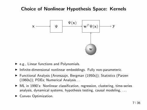
Choice of Nonlinear Hypothesis Space Kernels
x Ψ wTΨ(x) y
w
Ψ(x)
I eg Linear functions and Polynomials
I Infinite-dimensional nonlinear embeddings Fully non-parameteric
I Functional Analysis (Aronszajn Bergman (1950s)) Statistics (Parzen(1960s)) PDEs Numerical Analysis
I ML in 1990rsquos Nonlinear classification regression clustering time-seriesanalysis dynamical systems hypothesis testing causal modeling
I Convex Optimization
7 36
Choice of Nonlinear Hypothesis Space Kernels
x Ψ wTΨ(x) y
w
Ψ(x)
I eg Linear functions and Polynomials
I Infinite-dimensional nonlinear embeddings Fully non-parameteric
I Functional Analysis (Aronszajn Bergman (1950s)) Statistics (Parzen(1960s)) PDEs Numerical Analysis
I ML in 1990rsquos Nonlinear classification regression clustering time-seriesanalysis dynamical systems hypothesis testing causal modeling
I Convex Optimization
7 36
Choice of Nonlinear Hypothesis Space Deep Learning
x0 f1 f2 fL `
w1 w2 wL
z isin Rx1 x2 xLminus1 xL
I Compositions Raw data to higher abstractions (representation learning)
I Multilayer Perceptrons fl(xW) = σ(Wx) (sigmoids ReLU)I Turing (1950) In considering the functions of the mind or the brain we find certain operations which we can explain in
purely mechanical terms This we say does not correspond to the real mind it is a sort of skin which we must strip off if we are
to find the real mind Proceeding in this way do we ever come to the rdquorealrdquo mind or do we eventually come to the skin which
has nothing in it In the latter case the whole mind is mechanical
I Rosenblatt (1957) NYT 1958 New Navy Device Learns By Doing The Navy revealed the embryo of an electronic
computer today that it expects will be able to walk talk see write reproduce itself and be conscious of its existence Later
perceptrons will be able to recognize people and call out their names and instantly translate speech in one language to speech
and writing in another language it was predicted
I Perceptron (Minski and Pappert 1969) [Olarzan A Sociological Study 1996]I Backprop (1986) Reverse-mode differentiation (1960s-70s) CNNs (1980s 2012-)I Breadth-Width tradeoffsI Non-convex Optimization Domain-agnostic recipe
8 36
Choice of Nonlinear Hypothesis Space Deep Learning
x0 f1 f2 fL `
w1 w2 wL
z isin Rx1 x2 xLminus1 xL
I Compositions Raw data to higher abstractions (representation learning)I Multilayer Perceptrons fl(xW) = σ(Wx) (sigmoids ReLU)
I Turing (1950) In considering the functions of the mind or the brain we find certain operations which we can explain in
purely mechanical terms This we say does not correspond to the real mind it is a sort of skin which we must strip off if we are
to find the real mind Proceeding in this way do we ever come to the rdquorealrdquo mind or do we eventually come to the skin which
has nothing in it In the latter case the whole mind is mechanical
I Rosenblatt (1957) NYT 1958 New Navy Device Learns By Doing The Navy revealed the embryo of an electronic
computer today that it expects will be able to walk talk see write reproduce itself and be conscious of its existence Later
perceptrons will be able to recognize people and call out their names and instantly translate speech in one language to speech
and writing in another language it was predicted
I Perceptron (Minski and Pappert 1969) [Olarzan A Sociological Study 1996]I Backprop (1986) Reverse-mode differentiation (1960s-70s) CNNs (1980s 2012-)I Breadth-Width tradeoffsI Non-convex Optimization Domain-agnostic recipe
8 36
Choice of Nonlinear Hypothesis Space Deep Learning
x0 f1 f2 fL `
w1 w2 wL
z isin Rx1 x2 xLminus1 xL
I Compositions Raw data to higher abstractions (representation learning)I Multilayer Perceptrons fl(xW) = σ(Wx) (sigmoids ReLU)I Turing (1950) In considering the functions of the mind or the brain we find certain operations which we can explain in
purely mechanical terms This we say does not correspond to the real mind it is a sort of skin which we must strip off if we are
to find the real mind Proceeding in this way do we ever come to the rdquorealrdquo mind or do we eventually come to the skin which
has nothing in it In the latter case the whole mind is mechanical
I Rosenblatt (1957) NYT 1958 New Navy Device Learns By Doing The Navy revealed the embryo of an electronic
computer today that it expects will be able to walk talk see write reproduce itself and be conscious of its existence Later
perceptrons will be able to recognize people and call out their names and instantly translate speech in one language to speech
and writing in another language it was predicted
I Perceptron (Minski and Pappert 1969) [Olarzan A Sociological Study 1996]I Backprop (1986) Reverse-mode differentiation (1960s-70s) CNNs (1980s 2012-)I Breadth-Width tradeoffsI Non-convex Optimization Domain-agnostic recipe
8 36
Choice of Nonlinear Hypothesis Space Deep Learning
x0 f1 f2 fL `
w1 w2 wL
z isin Rx1 x2 xLminus1 xL
I Compositions Raw data to higher abstractions (representation learning)I Multilayer Perceptrons fl(xW) = σ(Wx) (sigmoids ReLU)I Turing (1950) In considering the functions of the mind or the brain we find certain operations which we can explain in
purely mechanical terms This we say does not correspond to the real mind it is a sort of skin which we must strip off if we are
to find the real mind Proceeding in this way do we ever come to the rdquorealrdquo mind or do we eventually come to the skin which
has nothing in it In the latter case the whole mind is mechanical
I Rosenblatt (1957) NYT 1958 New Navy Device Learns By Doing The Navy revealed the embryo of an electronic
computer today that it expects will be able to walk talk see write reproduce itself and be conscious of its existence Later
perceptrons will be able to recognize people and call out their names and instantly translate speech in one language to speech
and writing in another language it was predicted
I Perceptron (Minski and Pappert 1969) [Olarzan A Sociological Study 1996]I Backprop (1986) Reverse-mode differentiation (1960s-70s) CNNs (1980s 2012-)I Breadth-Width tradeoffsI Non-convex Optimization Domain-agnostic recipe
8 36
Choice of Nonlinear Hypothesis Space Deep Learning
x0 f1 f2 fL `
w1 w2 wL
z isin Rx1 x2 xLminus1 xL
I Compositions Raw data to higher abstractions (representation learning)I Multilayer Perceptrons fl(xW) = σ(Wx) (sigmoids ReLU)I Turing (1950) In considering the functions of the mind or the brain we find certain operations which we can explain in
purely mechanical terms This we say does not correspond to the real mind it is a sort of skin which we must strip off if we are
to find the real mind Proceeding in this way do we ever come to the rdquorealrdquo mind or do we eventually come to the skin which
has nothing in it In the latter case the whole mind is mechanical
I Rosenblatt (1957) NYT 1958 New Navy Device Learns By Doing The Navy revealed the embryo of an electronic
computer today that it expects will be able to walk talk see write reproduce itself and be conscious of its existence Later
perceptrons will be able to recognize people and call out their names and instantly translate speech in one language to speech
and writing in another language it was predicted
I Perceptron (Minski and Pappert 1969) [Olarzan A Sociological Study 1996]I Backprop (1986) Reverse-mode differentiation (1960s-70s) CNNs (1980s 2012-)
I Breadth-Width tradeoffsI Non-convex Optimization Domain-agnostic recipe
8 36
Choice of Nonlinear Hypothesis Space Deep Learning
x0 f1 f2 fL `
w1 w2 wL
z isin Rx1 x2 xLminus1 xL
I Compositions Raw data to higher abstractions (representation learning)I Multilayer Perceptrons fl(xW) = σ(Wx) (sigmoids ReLU)I Turing (1950) In considering the functions of the mind or the brain we find certain operations which we can explain in
purely mechanical terms This we say does not correspond to the real mind it is a sort of skin which we must strip off if we are
to find the real mind Proceeding in this way do we ever come to the rdquorealrdquo mind or do we eventually come to the skin which
has nothing in it In the latter case the whole mind is mechanical
I Rosenblatt (1957) NYT 1958 New Navy Device Learns By Doing The Navy revealed the embryo of an electronic
computer today that it expects will be able to walk talk see write reproduce itself and be conscious of its existence Later
perceptrons will be able to recognize people and call out their names and instantly translate speech in one language to speech
and writing in another language it was predicted
I Perceptron (Minski and Pappert 1969) [Olarzan A Sociological Study 1996]I Backprop (1986) Reverse-mode differentiation (1960s-70s) CNNs (1980s 2012-)I Breadth-Width tradeoffsI Non-convex Optimization Domain-agnostic recipe 8 36
Choice of Nonlinear Hypothesis Space Deep Learning
x0 f1 f2 fL `
w1 w2 wL
z isin Rx1 x2 xLminus1 xL
I Compositions Raw data to higher abstractions (representation learning)I Multilayer Perceptrons fl(xW) = σ(Wx) (sigmoids ReLU)I Turing (1950) In considering the functions of the mind or the brain we find certain operations which we can explain in
purely mechanical terms This we say does not correspond to the real mind it is a sort of skin which we must strip off if we are
to find the real mind Proceeding in this way do we ever come to the rdquorealrdquo mind or do we eventually come to the skin which
has nothing in it In the latter case the whole mind is mechanical
I Rosenblatt (1957) NYT 1958 New Navy Device Learns By Doing The Navy revealed the embryo of an electronic
computer today that it expects will be able to walk talk see write reproduce itself and be conscious of its existence Later
perceptrons will be able to recognize people and call out their names and instantly translate speech in one language to speech
and writing in another language it was predicted
I Perceptron (Minski and Pappert 1969) [Olarzan A Sociological Study 1996]I Backprop (1986) Reverse-mode differentiation (1960s-70s) CNNs (1980s 2012-)I Breadth-Width tradeoffsI Non-convex Optimization Domain-agnostic recipe 8 36
The Watershed Moment Imagenet 2012
I Many statistical and computational ingredientsndash Large datasets (ILSVRC since 2010)
ndash Large statistical capacity (12M images 60M params)ndash Distributed computationndash Depth Invariant feature learning (transferrable to other tasks)ndash Engineering Dropout ReLU
I Many astonishing results since then
9 36
The Watershed Moment Imagenet 2012
I Many statistical and computational ingredientsndash Large datasets (ILSVRC since 2010)ndash Large statistical capacity (12M images 60M params)
ndash Distributed computationndash Depth Invariant feature learning (transferrable to other tasks)ndash Engineering Dropout ReLU
I Many astonishing results since then
9 36
The Watershed Moment Imagenet 2012
I Many statistical and computational ingredientsndash Large datasets (ILSVRC since 2010)ndash Large statistical capacity (12M images 60M params)ndash Distributed computation
ndash Depth Invariant feature learning (transferrable to other tasks)ndash Engineering Dropout ReLU
I Many astonishing results since then
9 36
The Watershed Moment Imagenet 2012
I Many statistical and computational ingredientsndash Large datasets (ILSVRC since 2010)ndash Large statistical capacity (12M images 60M params)ndash Distributed computationndash Depth Invariant feature learning (transferrable to other tasks)
ndash Engineering Dropout ReLU I Many astonishing results since then
9 36
The Watershed Moment Imagenet 2012
I Many statistical and computational ingredientsndash Large datasets (ILSVRC since 2010)ndash Large statistical capacity (12M images 60M params)ndash Distributed computationndash Depth Invariant feature learning (transferrable to other tasks)ndash Engineering Dropout ReLU
I Many astonishing results since then
9 36
CNNs
10 36
Self-Driving Cars
Figure End-to-End Learning for Self-driving Cars Bojarski et al 2016
11 36

Choice of Nonlinear Hypothesis Space Kernels
x Ψ wTΨ(x) y
w
Ψ(x)
I eg Linear functions and Polynomials
I Infinite-dimensional nonlinear embeddings Fully non-parameteric
I Functional Analysis (Aronszajn Bergman (1950s)) Statistics (Parzen(1960s)) PDEs Numerical Analysis
I ML in 1990rsquos Nonlinear classification regression clustering time-seriesanalysis dynamical systems hypothesis testing causal modeling
I Convex Optimization
7 36
Choice of Nonlinear Hypothesis Space Deep Learning
x0 f1 f2 fL `
w1 w2 wL
z isin Rx1 x2 xLminus1 xL
I Compositions Raw data to higher abstractions (representation learning)
I Multilayer Perceptrons fl(xW) = σ(Wx) (sigmoids ReLU)I Turing (1950) In considering the functions of the mind or the brain we find certain operations which we can explain in
purely mechanical terms This we say does not correspond to the real mind it is a sort of skin which we must strip off if we are
to find the real mind Proceeding in this way do we ever come to the rdquorealrdquo mind or do we eventually come to the skin which
has nothing in it In the latter case the whole mind is mechanical
I Rosenblatt (1957) NYT 1958 New Navy Device Learns By Doing The Navy revealed the embryo of an electronic
computer today that it expects will be able to walk talk see write reproduce itself and be conscious of its existence Later
perceptrons will be able to recognize people and call out their names and instantly translate speech in one language to speech
and writing in another language it was predicted
I Perceptron (Minski and Pappert 1969) [Olarzan A Sociological Study 1996]I Backprop (1986) Reverse-mode differentiation (1960s-70s) CNNs (1980s 2012-)I Breadth-Width tradeoffsI Non-convex Optimization Domain-agnostic recipe
8 36
Choice of Nonlinear Hypothesis Space Deep Learning
x0 f1 f2 fL `
w1 w2 wL
z isin Rx1 x2 xLminus1 xL
I Compositions Raw data to higher abstractions (representation learning)I Multilayer Perceptrons fl(xW) = σ(Wx) (sigmoids ReLU)
I Turing (1950) In considering the functions of the mind or the brain we find certain operations which we can explain in
purely mechanical terms This we say does not correspond to the real mind it is a sort of skin which we must strip off if we are
to find the real mind Proceeding in this way do we ever come to the rdquorealrdquo mind or do we eventually come to the skin which
has nothing in it In the latter case the whole mind is mechanical
I Rosenblatt (1957) NYT 1958 New Navy Device Learns By Doing The Navy revealed the embryo of an electronic
computer today that it expects will be able to walk talk see write reproduce itself and be conscious of its existence Later
perceptrons will be able to recognize people and call out their names and instantly translate speech in one language to speech
and writing in another language it was predicted
I Perceptron (Minski and Pappert 1969) [Olarzan A Sociological Study 1996]I Backprop (1986) Reverse-mode differentiation (1960s-70s) CNNs (1980s 2012-)I Breadth-Width tradeoffsI Non-convex Optimization Domain-agnostic recipe
8 36
Choice of Nonlinear Hypothesis Space Deep Learning
x0 f1 f2 fL `
w1 w2 wL
z isin Rx1 x2 xLminus1 xL
I Compositions Raw data to higher abstractions (representation learning)I Multilayer Perceptrons fl(xW) = σ(Wx) (sigmoids ReLU)I Turing (1950) In considering the functions of the mind or the brain we find certain operations which we can explain in
purely mechanical terms This we say does not correspond to the real mind it is a sort of skin which we must strip off if we are
to find the real mind Proceeding in this way do we ever come to the rdquorealrdquo mind or do we eventually come to the skin which
has nothing in it In the latter case the whole mind is mechanical
I Rosenblatt (1957) NYT 1958 New Navy Device Learns By Doing The Navy revealed the embryo of an electronic
computer today that it expects will be able to walk talk see write reproduce itself and be conscious of its existence Later
perceptrons will be able to recognize people and call out their names and instantly translate speech in one language to speech
and writing in another language it was predicted
I Perceptron (Minski and Pappert 1969) [Olarzan A Sociological Study 1996]I Backprop (1986) Reverse-mode differentiation (1960s-70s) CNNs (1980s 2012-)I Breadth-Width tradeoffsI Non-convex Optimization Domain-agnostic recipe
8 36
Choice of Nonlinear Hypothesis Space Deep Learning
x0 f1 f2 fL `
w1 w2 wL
z isin Rx1 x2 xLminus1 xL
I Compositions Raw data to higher abstractions (representation learning)I Multilayer Perceptrons fl(xW) = σ(Wx) (sigmoids ReLU)I Turing (1950) In considering the functions of the mind or the brain we find certain operations which we can explain in
purely mechanical terms This we say does not correspond to the real mind it is a sort of skin which we must strip off if we are
to find the real mind Proceeding in this way do we ever come to the rdquorealrdquo mind or do we eventually come to the skin which
has nothing in it In the latter case the whole mind is mechanical
I Rosenblatt (1957) NYT 1958 New Navy Device Learns By Doing The Navy revealed the embryo of an electronic
computer today that it expects will be able to walk talk see write reproduce itself and be conscious of its existence Later
perceptrons will be able to recognize people and call out their names and instantly translate speech in one language to speech
and writing in another language it was predicted
I Perceptron (Minski and Pappert 1969) [Olarzan A Sociological Study 1996]I Backprop (1986) Reverse-mode differentiation (1960s-70s) CNNs (1980s 2012-)I Breadth-Width tradeoffsI Non-convex Optimization Domain-agnostic recipe
8 36
Choice of Nonlinear Hypothesis Space Deep Learning
x0 f1 f2 fL `
w1 w2 wL
z isin Rx1 x2 xLminus1 xL
I Compositions Raw data to higher abstractions (representation learning)I Multilayer Perceptrons fl(xW) = σ(Wx) (sigmoids ReLU)I Turing (1950) In considering the functions of the mind or the brain we find certain operations which we can explain in
purely mechanical terms This we say does not correspond to the real mind it is a sort of skin which we must strip off if we are
to find the real mind Proceeding in this way do we ever come to the rdquorealrdquo mind or do we eventually come to the skin which
has nothing in it In the latter case the whole mind is mechanical
I Rosenblatt (1957) NYT 1958 New Navy Device Learns By Doing The Navy revealed the embryo of an electronic
computer today that it expects will be able to walk talk see write reproduce itself and be conscious of its existence Later
perceptrons will be able to recognize people and call out their names and instantly translate speech in one language to speech
and writing in another language it was predicted
I Perceptron (Minski and Pappert 1969) [Olarzan A Sociological Study 1996]I Backprop (1986) Reverse-mode differentiation (1960s-70s) CNNs (1980s 2012-)
I Breadth-Width tradeoffsI Non-convex Optimization Domain-agnostic recipe
8 36
Choice of Nonlinear Hypothesis Space Deep Learning
x0 f1 f2 fL `
w1 w2 wL
z isin Rx1 x2 xLminus1 xL
I Compositions Raw data to higher abstractions (representation learning)I Multilayer Perceptrons fl(xW) = σ(Wx) (sigmoids ReLU)I Turing (1950) In considering the functions of the mind or the brain we find certain operations which we can explain in
purely mechanical terms This we say does not correspond to the real mind it is a sort of skin which we must strip off if we are
to find the real mind Proceeding in this way do we ever come to the rdquorealrdquo mind or do we eventually come to the skin which
has nothing in it In the latter case the whole mind is mechanical
I Rosenblatt (1957) NYT 1958 New Navy Device Learns By Doing The Navy revealed the embryo of an electronic
computer today that it expects will be able to walk talk see write reproduce itself and be conscious of its existence Later
perceptrons will be able to recognize people and call out their names and instantly translate speech in one language to speech
and writing in another language it was predicted
I Perceptron (Minski and Pappert 1969) [Olarzan A Sociological Study 1996]I Backprop (1986) Reverse-mode differentiation (1960s-70s) CNNs (1980s 2012-)I Breadth-Width tradeoffsI Non-convex Optimization Domain-agnostic recipe 8 36
Choice of Nonlinear Hypothesis Space Deep Learning
x0 f1 f2 fL `
w1 w2 wL
z isin Rx1 x2 xLminus1 xL
I Compositions Raw data to higher abstractions (representation learning)I Multilayer Perceptrons fl(xW) = σ(Wx) (sigmoids ReLU)I Turing (1950) In considering the functions of the mind or the brain we find certain operations which we can explain in
purely mechanical terms This we say does not correspond to the real mind it is a sort of skin which we must strip off if we are
to find the real mind Proceeding in this way do we ever come to the rdquorealrdquo mind or do we eventually come to the skin which
has nothing in it In the latter case the whole mind is mechanical
I Rosenblatt (1957) NYT 1958 New Navy Device Learns By Doing The Navy revealed the embryo of an electronic
computer today that it expects will be able to walk talk see write reproduce itself and be conscious of its existence Later
perceptrons will be able to recognize people and call out their names and instantly translate speech in one language to speech
and writing in another language it was predicted
I Perceptron (Minski and Pappert 1969) [Olarzan A Sociological Study 1996]I Backprop (1986) Reverse-mode differentiation (1960s-70s) CNNs (1980s 2012-)I Breadth-Width tradeoffsI Non-convex Optimization Domain-agnostic recipe 8 36
The Watershed Moment Imagenet 2012
I Many statistical and computational ingredientsndash Large datasets (ILSVRC since 2010)
ndash Large statistical capacity (12M images 60M params)ndash Distributed computationndash Depth Invariant feature learning (transferrable to other tasks)ndash Engineering Dropout ReLU
I Many astonishing results since then
9 36
The Watershed Moment Imagenet 2012
I Many statistical and computational ingredientsndash Large datasets (ILSVRC since 2010)ndash Large statistical capacity (12M images 60M params)
ndash Distributed computationndash Depth Invariant feature learning (transferrable to other tasks)ndash Engineering Dropout ReLU
I Many astonishing results since then
9 36
The Watershed Moment Imagenet 2012
I Many statistical and computational ingredientsndash Large datasets (ILSVRC since 2010)ndash Large statistical capacity (12M images 60M params)ndash Distributed computation
ndash Depth Invariant feature learning (transferrable to other tasks)ndash Engineering Dropout ReLU
I Many astonishing results since then
9 36
The Watershed Moment Imagenet 2012
I Many statistical and computational ingredientsndash Large datasets (ILSVRC since 2010)ndash Large statistical capacity (12M images 60M params)ndash Distributed computationndash Depth Invariant feature learning (transferrable to other tasks)
ndash Engineering Dropout ReLU I Many astonishing results since then
9 36
The Watershed Moment Imagenet 2012
I Many statistical and computational ingredientsndash Large datasets (ILSVRC since 2010)ndash Large statistical capacity (12M images 60M params)ndash Distributed computationndash Depth Invariant feature learning (transferrable to other tasks)ndash Engineering Dropout ReLU
I Many astonishing results since then
9 36
CNNs
10 36
Self-Driving Cars
Figure End-to-End Learning for Self-driving Cars Bojarski et al 2016
11 36

Choice of Nonlinear Hypothesis Space Deep Learning
x0 f1 f2 fL `
w1 w2 wL
z isin Rx1 x2 xLminus1 xL
I Compositions Raw data to higher abstractions (representation learning)I Multilayer Perceptrons fl(xW) = σ(Wx) (sigmoids ReLU)
I Turing (1950) In considering the functions of the mind or the brain we find certain operations which we can explain in
purely mechanical terms This we say does not correspond to the real mind it is a sort of skin which we must strip off if we are
to find the real mind Proceeding in this way do we ever come to the rdquorealrdquo mind or do we eventually come to the skin which
has nothing in it In the latter case the whole mind is mechanical
I Rosenblatt (1957) NYT 1958 New Navy Device Learns By Doing The Navy revealed the embryo of an electronic
computer today that it expects will be able to walk talk see write reproduce itself and be conscious of its existence Later
perceptrons will be able to recognize people and call out their names and instantly translate speech in one language to speech
and writing in another language it was predicted
I Perceptron (Minski and Pappert 1969) [Olarzan A Sociological Study 1996]I Backprop (1986) Reverse-mode differentiation (1960s-70s) CNNs (1980s 2012-)I Breadth-Width tradeoffsI Non-convex Optimization Domain-agnostic recipe
8 36
Choice of Nonlinear Hypothesis Space Deep Learning
x0 f1 f2 fL `
w1 w2 wL
z isin Rx1 x2 xLminus1 xL
I Compositions Raw data to higher abstractions (representation learning)I Multilayer Perceptrons fl(xW) = σ(Wx) (sigmoids ReLU)I Turing (1950) In considering the functions of the mind or the brain we find certain operations which we can explain in
purely mechanical terms This we say does not correspond to the real mind it is a sort of skin which we must strip off if we are
to find the real mind Proceeding in this way do we ever come to the rdquorealrdquo mind or do we eventually come to the skin which
has nothing in it In the latter case the whole mind is mechanical
I Rosenblatt (1957) NYT 1958 New Navy Device Learns By Doing The Navy revealed the embryo of an electronic
computer today that it expects will be able to walk talk see write reproduce itself and be conscious of its existence Later
perceptrons will be able to recognize people and call out their names and instantly translate speech in one language to speech
and writing in another language it was predicted
I Perceptron (Minski and Pappert 1969) [Olarzan A Sociological Study 1996]I Backprop (1986) Reverse-mode differentiation (1960s-70s) CNNs (1980s 2012-)I Breadth-Width tradeoffsI Non-convex Optimization Domain-agnostic recipe
8 36
Choice of Nonlinear Hypothesis Space Deep Learning
x0 f1 f2 fL `
w1 w2 wL
z isin Rx1 x2 xLminus1 xL
I Compositions Raw data to higher abstractions (representation learning)I Multilayer Perceptrons fl(xW) = σ(Wx) (sigmoids ReLU)I Turing (1950) In considering the functions of the mind or the brain we find certain operations which we can explain in
purely mechanical terms This we say does not correspond to the real mind it is a sort of skin which we must strip off if we are
to find the real mind Proceeding in this way do we ever come to the rdquorealrdquo mind or do we eventually come to the skin which
has nothing in it In the latter case the whole mind is mechanical
I Rosenblatt (1957) NYT 1958 New Navy Device Learns By Doing The Navy revealed the embryo of an electronic
computer today that it expects will be able to walk talk see write reproduce itself and be conscious of its existence Later
perceptrons will be able to recognize people and call out their names and instantly translate speech in one language to speech
and writing in another language it was predicted
I Perceptron (Minski and Pappert 1969) [Olarzan A Sociological Study 1996]I Backprop (1986) Reverse-mode differentiation (1960s-70s) CNNs (1980s 2012-)I Breadth-Width tradeoffsI Non-convex Optimization Domain-agnostic recipe
8 36
Choice of Nonlinear Hypothesis Space Deep Learning
x0 f1 f2 fL `
w1 w2 wL
z isin Rx1 x2 xLminus1 xL
I Compositions Raw data to higher abstractions (representation learning)I Multilayer Perceptrons fl(xW) = σ(Wx) (sigmoids ReLU)I Turing (1950) In considering the functions of the mind or the brain we find certain operations which we can explain in
purely mechanical terms This we say does not correspond to the real mind it is a sort of skin which we must strip off if we are
to find the real mind Proceeding in this way do we ever come to the rdquorealrdquo mind or do we eventually come to the skin which
has nothing in it In the latter case the whole mind is mechanical
I Rosenblatt (1957) NYT 1958 New Navy Device Learns By Doing The Navy revealed the embryo of an electronic
computer today that it expects will be able to walk talk see write reproduce itself and be conscious of its existence Later
perceptrons will be able to recognize people and call out their names and instantly translate speech in one language to speech
and writing in another language it was predicted
I Perceptron (Minski and Pappert 1969) [Olarzan A Sociological Study 1996]I Backprop (1986) Reverse-mode differentiation (1960s-70s) CNNs (1980s 2012-)
I Breadth-Width tradeoffsI Non-convex Optimization Domain-agnostic recipe
8 36
Choice of Nonlinear Hypothesis Space Deep Learning
x0 f1 f2 fL `
w1 w2 wL
z isin Rx1 x2 xLminus1 xL
I Compositions Raw data to higher abstractions (representation learning)I Multilayer Perceptrons fl(xW) = σ(Wx) (sigmoids ReLU)I Turing (1950) In considering the functions of the mind or the brain we find certain operations which we can explain in
purely mechanical terms This we say does not correspond to the real mind it is a sort of skin which we must strip off if we are
to find the real mind Proceeding in this way do we ever come to the rdquorealrdquo mind or do we eventually come to the skin which
has nothing in it In the latter case the whole mind is mechanical
I Rosenblatt (1957) NYT 1958 New Navy Device Learns By Doing The Navy revealed the embryo of an electronic
computer today that it expects will be able to walk talk see write reproduce itself and be conscious of its existence Later
perceptrons will be able to recognize people and call out their names and instantly translate speech in one language to speech
and writing in another language it was predicted
I Perceptron (Minski and Pappert 1969) [Olarzan A Sociological Study 1996]I Backprop (1986) Reverse-mode differentiation (1960s-70s) CNNs (1980s 2012-)I Breadth-Width tradeoffsI Non-convex Optimization Domain-agnostic recipe 8 36
Choice of Nonlinear Hypothesis Space Deep Learning
x0 f1 f2 fL `
w1 w2 wL
z isin Rx1 x2 xLminus1 xL
I Compositions Raw data to higher abstractions (representation learning)I Multilayer Perceptrons fl(xW) = σ(Wx) (sigmoids ReLU)I Turing (1950) In considering the functions of the mind or the brain we find certain operations which we can explain in
purely mechanical terms This we say does not correspond to the real mind it is a sort of skin which we must strip off if we are
to find the real mind Proceeding in this way do we ever come to the rdquorealrdquo mind or do we eventually come to the skin which
has nothing in it In the latter case the whole mind is mechanical
I Rosenblatt (1957) NYT 1958 New Navy Device Learns By Doing The Navy revealed the embryo of an electronic
computer today that it expects will be able to walk talk see write reproduce itself and be conscious of its existence Later
perceptrons will be able to recognize people and call out their names and instantly translate speech in one language to speech
and writing in another language it was predicted
I Perceptron (Minski and Pappert 1969) [Olarzan A Sociological Study 1996]I Backprop (1986) Reverse-mode differentiation (1960s-70s) CNNs (1980s 2012-)I Breadth-Width tradeoffsI Non-convex Optimization Domain-agnostic recipe 8 36
The Watershed Moment Imagenet 2012
I Many statistical and computational ingredientsndash Large datasets (ILSVRC since 2010)
ndash Large statistical capacity (12M images 60M params)ndash Distributed computationndash Depth Invariant feature learning (transferrable to other tasks)ndash Engineering Dropout ReLU
I Many astonishing results since then
9 36
The Watershed Moment Imagenet 2012
I Many statistical and computational ingredientsndash Large datasets (ILSVRC since 2010)ndash Large statistical capacity (12M images 60M params)
ndash Distributed computationndash Depth Invariant feature learning (transferrable to other tasks)ndash Engineering Dropout ReLU
I Many astonishing results since then
9 36
The Watershed Moment Imagenet 2012
I Many statistical and computational ingredientsndash Large datasets (ILSVRC since 2010)ndash Large statistical capacity (12M images 60M params)ndash Distributed computation
ndash Depth Invariant feature learning (transferrable to other tasks)ndash Engineering Dropout ReLU
I Many astonishing results since then
9 36
The Watershed Moment Imagenet 2012
I Many statistical and computational ingredientsndash Large datasets (ILSVRC since 2010)ndash Large statistical capacity (12M images 60M params)ndash Distributed computationndash Depth Invariant feature learning (transferrable to other tasks)
ndash Engineering Dropout ReLU I Many astonishing results since then
9 36
The Watershed Moment Imagenet 2012
I Many statistical and computational ingredientsndash Large datasets (ILSVRC since 2010)ndash Large statistical capacity (12M images 60M params)ndash Distributed computationndash Depth Invariant feature learning (transferrable to other tasks)ndash Engineering Dropout ReLU
I Many astonishing results since then
9 36
CNNs
10 36
Self-Driving Cars
Figure End-to-End Learning for Self-driving Cars Bojarski et al 2016
11 36
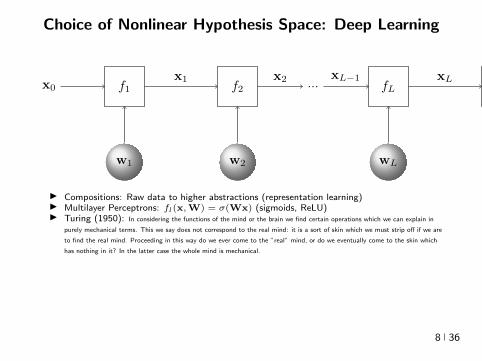
Choice of Nonlinear Hypothesis Space Deep Learning
x0 f1 f2 fL `
w1 w2 wL
z isin Rx1 x2 xLminus1 xL
I Compositions Raw data to higher abstractions (representation learning)I Multilayer Perceptrons fl(xW) = σ(Wx) (sigmoids ReLU)I Turing (1950) In considering the functions of the mind or the brain we find certain operations which we can explain in
purely mechanical terms This we say does not correspond to the real mind it is a sort of skin which we must strip off if we are
to find the real mind Proceeding in this way do we ever come to the rdquorealrdquo mind or do we eventually come to the skin which
has nothing in it In the latter case the whole mind is mechanical
I Rosenblatt (1957) NYT 1958 New Navy Device Learns By Doing The Navy revealed the embryo of an electronic
computer today that it expects will be able to walk talk see write reproduce itself and be conscious of its existence Later
perceptrons will be able to recognize people and call out their names and instantly translate speech in one language to speech
and writing in another language it was predicted
I Perceptron (Minski and Pappert 1969) [Olarzan A Sociological Study 1996]I Backprop (1986) Reverse-mode differentiation (1960s-70s) CNNs (1980s 2012-)I Breadth-Width tradeoffsI Non-convex Optimization Domain-agnostic recipe
8 36
Choice of Nonlinear Hypothesis Space Deep Learning
x0 f1 f2 fL `
w1 w2 wL
z isin Rx1 x2 xLminus1 xL
I Compositions Raw data to higher abstractions (representation learning)I Multilayer Perceptrons fl(xW) = σ(Wx) (sigmoids ReLU)I Turing (1950) In considering the functions of the mind or the brain we find certain operations which we can explain in
purely mechanical terms This we say does not correspond to the real mind it is a sort of skin which we must strip off if we are
to find the real mind Proceeding in this way do we ever come to the rdquorealrdquo mind or do we eventually come to the skin which
has nothing in it In the latter case the whole mind is mechanical
I Rosenblatt (1957) NYT 1958 New Navy Device Learns By Doing The Navy revealed the embryo of an electronic
computer today that it expects will be able to walk talk see write reproduce itself and be conscious of its existence Later
perceptrons will be able to recognize people and call out their names and instantly translate speech in one language to speech
and writing in another language it was predicted
I Perceptron (Minski and Pappert 1969) [Olarzan A Sociological Study 1996]I Backprop (1986) Reverse-mode differentiation (1960s-70s) CNNs (1980s 2012-)
I Breadth-Width tradeoffsI Non-convex Optimization Domain-agnostic recipe
8 36
Choice of Nonlinear Hypothesis Space Deep Learning
x0 f1 f2 fL `
w1 w2 wL
z isin Rx1 x2 xLminus1 xL
I Compositions Raw data to higher abstractions (representation learning)I Multilayer Perceptrons fl(xW) = σ(Wx) (sigmoids ReLU)I Turing (1950) In considering the functions of the mind or the brain we find certain operations which we can explain in
purely mechanical terms This we say does not correspond to the real mind it is a sort of skin which we must strip off if we are
to find the real mind Proceeding in this way do we ever come to the rdquorealrdquo mind or do we eventually come to the skin which
has nothing in it In the latter case the whole mind is mechanical
I Rosenblatt (1957) NYT 1958 New Navy Device Learns By Doing The Navy revealed the embryo of an electronic
computer today that it expects will be able to walk talk see write reproduce itself and be conscious of its existence Later
perceptrons will be able to recognize people and call out their names and instantly translate speech in one language to speech
and writing in another language it was predicted
I Perceptron (Minski and Pappert 1969) [Olarzan A Sociological Study 1996]I Backprop (1986) Reverse-mode differentiation (1960s-70s) CNNs (1980s 2012-)I Breadth-Width tradeoffsI Non-convex Optimization Domain-agnostic recipe 8 36
Choice of Nonlinear Hypothesis Space Deep Learning
x0 f1 f2 fL `
w1 w2 wL
z isin Rx1 x2 xLminus1 xL
I Compositions Raw data to higher abstractions (representation learning)I Multilayer Perceptrons fl(xW) = σ(Wx) (sigmoids ReLU)I Turing (1950) In considering the functions of the mind or the brain we find certain operations which we can explain in
purely mechanical terms This we say does not correspond to the real mind it is a sort of skin which we must strip off if we are
to find the real mind Proceeding in this way do we ever come to the rdquorealrdquo mind or do we eventually come to the skin which
has nothing in it In the latter case the whole mind is mechanical
I Rosenblatt (1957) NYT 1958 New Navy Device Learns By Doing The Navy revealed the embryo of an electronic
computer today that it expects will be able to walk talk see write reproduce itself and be conscious of its existence Later
perceptrons will be able to recognize people and call out their names and instantly translate speech in one language to speech
and writing in another language it was predicted
I Perceptron (Minski and Pappert 1969) [Olarzan A Sociological Study 1996]I Backprop (1986) Reverse-mode differentiation (1960s-70s) CNNs (1980s 2012-)I Breadth-Width tradeoffsI Non-convex Optimization Domain-agnostic recipe 8 36
The Watershed Moment Imagenet 2012
I Many statistical and computational ingredientsndash Large datasets (ILSVRC since 2010)
ndash Large statistical capacity (12M images 60M params)ndash Distributed computationndash Depth Invariant feature learning (transferrable to other tasks)ndash Engineering Dropout ReLU
I Many astonishing results since then
9 36
The Watershed Moment Imagenet 2012
I Many statistical and computational ingredientsndash Large datasets (ILSVRC since 2010)ndash Large statistical capacity (12M images 60M params)
ndash Distributed computationndash Depth Invariant feature learning (transferrable to other tasks)ndash Engineering Dropout ReLU
I Many astonishing results since then
9 36
The Watershed Moment Imagenet 2012
I Many statistical and computational ingredientsndash Large datasets (ILSVRC since 2010)ndash Large statistical capacity (12M images 60M params)ndash Distributed computation
ndash Depth Invariant feature learning (transferrable to other tasks)ndash Engineering Dropout ReLU
I Many astonishing results since then
9 36
The Watershed Moment Imagenet 2012
I Many statistical and computational ingredientsndash Large datasets (ILSVRC since 2010)ndash Large statistical capacity (12M images 60M params)ndash Distributed computationndash Depth Invariant feature learning (transferrable to other tasks)
ndash Engineering Dropout ReLU I Many astonishing results since then
9 36
The Watershed Moment Imagenet 2012
I Many statistical and computational ingredientsndash Large datasets (ILSVRC since 2010)ndash Large statistical capacity (12M images 60M params)ndash Distributed computationndash Depth Invariant feature learning (transferrable to other tasks)ndash Engineering Dropout ReLU
I Many astonishing results since then
9 36
CNNs
10 36
Self-Driving Cars
Figure End-to-End Learning for Self-driving Cars Bojarski et al 2016
11 36
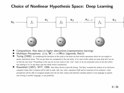
Choice of Nonlinear Hypothesis Space Deep Learning
x0 f1 f2 fL `
w1 w2 wL
z isin Rx1 x2 xLminus1 xL
I Compositions Raw data to higher abstractions (representation learning)I Multilayer Perceptrons fl(xW) = σ(Wx) (sigmoids ReLU)I Turing (1950) In considering the functions of the mind or the brain we find certain operations which we can explain in
purely mechanical terms This we say does not correspond to the real mind it is a sort of skin which we must strip off if we are
to find the real mind Proceeding in this way do we ever come to the rdquorealrdquo mind or do we eventually come to the skin which
has nothing in it In the latter case the whole mind is mechanical
I Rosenblatt (1957) NYT 1958 New Navy Device Learns By Doing The Navy revealed the embryo of an electronic
computer today that it expects will be able to walk talk see write reproduce itself and be conscious of its existence Later
perceptrons will be able to recognize people and call out their names and instantly translate speech in one language to speech
and writing in another language it was predicted
I Perceptron (Minski and Pappert 1969) [Olarzan A Sociological Study 1996]I Backprop (1986) Reverse-mode differentiation (1960s-70s) CNNs (1980s 2012-)I Breadth-Width tradeoffsI Non-convex Optimization Domain-agnostic recipe
8 36
Choice of Nonlinear Hypothesis Space Deep Learning
x0 f1 f2 fL `
w1 w2 wL
z isin Rx1 x2 xLminus1 xL
I Compositions Raw data to higher abstractions (representation learning)I Multilayer Perceptrons fl(xW) = σ(Wx) (sigmoids ReLU)I Turing (1950) In considering the functions of the mind or the brain we find certain operations which we can explain in
purely mechanical terms This we say does not correspond to the real mind it is a sort of skin which we must strip off if we are
to find the real mind Proceeding in this way do we ever come to the rdquorealrdquo mind or do we eventually come to the skin which
has nothing in it In the latter case the whole mind is mechanical
I Rosenblatt (1957) NYT 1958 New Navy Device Learns By Doing The Navy revealed the embryo of an electronic
computer today that it expects will be able to walk talk see write reproduce itself and be conscious of its existence Later
perceptrons will be able to recognize people and call out their names and instantly translate speech in one language to speech
and writing in another language it was predicted
I Perceptron (Minski and Pappert 1969) [Olarzan A Sociological Study 1996]I Backprop (1986) Reverse-mode differentiation (1960s-70s) CNNs (1980s 2012-)
I Breadth-Width tradeoffsI Non-convex Optimization Domain-agnostic recipe
8 36
Choice of Nonlinear Hypothesis Space Deep Learning
x0 f1 f2 fL `
w1 w2 wL
z isin Rx1 x2 xLminus1 xL
I Compositions Raw data to higher abstractions (representation learning)I Multilayer Perceptrons fl(xW) = σ(Wx) (sigmoids ReLU)I Turing (1950) In considering the functions of the mind or the brain we find certain operations which we can explain in
purely mechanical terms This we say does not correspond to the real mind it is a sort of skin which we must strip off if we are
to find the real mind Proceeding in this way do we ever come to the rdquorealrdquo mind or do we eventually come to the skin which
has nothing in it In the latter case the whole mind is mechanical
I Rosenblatt (1957) NYT 1958 New Navy Device Learns By Doing The Navy revealed the embryo of an electronic
computer today that it expects will be able to walk talk see write reproduce itself and be conscious of its existence Later
perceptrons will be able to recognize people and call out their names and instantly translate speech in one language to speech
and writing in another language it was predicted
I Perceptron (Minski and Pappert 1969) [Olarzan A Sociological Study 1996]I Backprop (1986) Reverse-mode differentiation (1960s-70s) CNNs (1980s 2012-)I Breadth-Width tradeoffsI Non-convex Optimization Domain-agnostic recipe 8 36
Choice of Nonlinear Hypothesis Space Deep Learning
x0 f1 f2 fL `
w1 w2 wL
z isin Rx1 x2 xLminus1 xL
I Compositions Raw data to higher abstractions (representation learning)I Multilayer Perceptrons fl(xW) = σ(Wx) (sigmoids ReLU)I Turing (1950) In considering the functions of the mind or the brain we find certain operations which we can explain in
purely mechanical terms This we say does not correspond to the real mind it is a sort of skin which we must strip off if we are
to find the real mind Proceeding in this way do we ever come to the rdquorealrdquo mind or do we eventually come to the skin which
has nothing in it In the latter case the whole mind is mechanical
I Rosenblatt (1957) NYT 1958 New Navy Device Learns By Doing The Navy revealed the embryo of an electronic
computer today that it expects will be able to walk talk see write reproduce itself and be conscious of its existence Later
perceptrons will be able to recognize people and call out their names and instantly translate speech in one language to speech
and writing in another language it was predicted
I Perceptron (Minski and Pappert 1969) [Olarzan A Sociological Study 1996]I Backprop (1986) Reverse-mode differentiation (1960s-70s) CNNs (1980s 2012-)I Breadth-Width tradeoffsI Non-convex Optimization Domain-agnostic recipe 8 36
The Watershed Moment Imagenet 2012
I Many statistical and computational ingredientsndash Large datasets (ILSVRC since 2010)
ndash Large statistical capacity (12M images 60M params)ndash Distributed computationndash Depth Invariant feature learning (transferrable to other tasks)ndash Engineering Dropout ReLU
I Many astonishing results since then
9 36
The Watershed Moment Imagenet 2012
I Many statistical and computational ingredientsndash Large datasets (ILSVRC since 2010)ndash Large statistical capacity (12M images 60M params)
ndash Distributed computationndash Depth Invariant feature learning (transferrable to other tasks)ndash Engineering Dropout ReLU
I Many astonishing results since then
9 36
The Watershed Moment Imagenet 2012
I Many statistical and computational ingredientsndash Large datasets (ILSVRC since 2010)ndash Large statistical capacity (12M images 60M params)ndash Distributed computation
ndash Depth Invariant feature learning (transferrable to other tasks)ndash Engineering Dropout ReLU
I Many astonishing results since then
9 36
The Watershed Moment Imagenet 2012
I Many statistical and computational ingredientsndash Large datasets (ILSVRC since 2010)ndash Large statistical capacity (12M images 60M params)ndash Distributed computationndash Depth Invariant feature learning (transferrable to other tasks)
ndash Engineering Dropout ReLU I Many astonishing results since then
9 36
The Watershed Moment Imagenet 2012
I Many statistical and computational ingredientsndash Large datasets (ILSVRC since 2010)ndash Large statistical capacity (12M images 60M params)ndash Distributed computationndash Depth Invariant feature learning (transferrable to other tasks)ndash Engineering Dropout ReLU
I Many astonishing results since then
9 36
CNNs
10 36
Self-Driving Cars
Figure End-to-End Learning for Self-driving Cars Bojarski et al 2016
11 36

Choice of Nonlinear Hypothesis Space Deep Learning
x0 f1 f2 fL `
w1 w2 wL
z isin Rx1 x2 xLminus1 xL
I Compositions Raw data to higher abstractions (representation learning)I Multilayer Perceptrons fl(xW) = σ(Wx) (sigmoids ReLU)I Turing (1950) In considering the functions of the mind or the brain we find certain operations which we can explain in
purely mechanical terms This we say does not correspond to the real mind it is a sort of skin which we must strip off if we are
to find the real mind Proceeding in this way do we ever come to the rdquorealrdquo mind or do we eventually come to the skin which
has nothing in it In the latter case the whole mind is mechanical
I Rosenblatt (1957) NYT 1958 New Navy Device Learns By Doing The Navy revealed the embryo of an electronic
computer today that it expects will be able to walk talk see write reproduce itself and be conscious of its existence Later
perceptrons will be able to recognize people and call out their names and instantly translate speech in one language to speech
and writing in another language it was predicted
I Perceptron (Minski and Pappert 1969) [Olarzan A Sociological Study 1996]I Backprop (1986) Reverse-mode differentiation (1960s-70s) CNNs (1980s 2012-)I Breadth-Width tradeoffsI Non-convex Optimization Domain-agnostic recipe 8 36
The Watershed Moment Imagenet 2012
I Many statistical and computational ingredientsndash Large datasets (ILSVRC since 2010)
ndash Large statistical capacity (12M images 60M params)ndash Distributed computationndash Depth Invariant feature learning (transferrable to other tasks)ndash Engineering Dropout ReLU
I Many astonishing results since then
9 36
The Watershed Moment Imagenet 2012
I Many statistical and computational ingredientsndash Large datasets (ILSVRC since 2010)ndash Large statistical capacity (12M images 60M params)
ndash Distributed computationndash Depth Invariant feature learning (transferrable to other tasks)ndash Engineering Dropout ReLU
I Many astonishing results since then
9 36
The Watershed Moment Imagenet 2012
I Many statistical and computational ingredientsndash Large datasets (ILSVRC since 2010)ndash Large statistical capacity (12M images 60M params)ndash Distributed computation
ndash Depth Invariant feature learning (transferrable to other tasks)ndash Engineering Dropout ReLU
I Many astonishing results since then
9 36
The Watershed Moment Imagenet 2012
I Many statistical and computational ingredientsndash Large datasets (ILSVRC since 2010)ndash Large statistical capacity (12M images 60M params)ndash Distributed computationndash Depth Invariant feature learning (transferrable to other tasks)
ndash Engineering Dropout ReLU I Many astonishing results since then
9 36
The Watershed Moment Imagenet 2012
I Many statistical and computational ingredientsndash Large datasets (ILSVRC since 2010)ndash Large statistical capacity (12M images 60M params)ndash Distributed computationndash Depth Invariant feature learning (transferrable to other tasks)ndash Engineering Dropout ReLU
I Many astonishing results since then
9 36
CNNs
10 36
Self-Driving Cars
Figure End-to-End Learning for Self-driving Cars Bojarski et al 2016
11 36
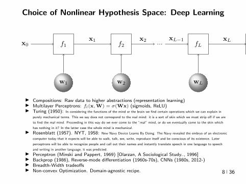
Choice of Nonlinear Hypothesis Space Deep Learning
x0 f1 f2 fL `
w1 w2 wL
z isin Rx1 x2 xLminus1 xL
I Compositions Raw data to higher abstractions (representation learning)I Multilayer Perceptrons fl(xW) = σ(Wx) (sigmoids ReLU)I Turing (1950) In considering the functions of the mind or the brain we find certain operations which we can explain in
purely mechanical terms This we say does not correspond to the real mind it is a sort of skin which we must strip off if we are
to find the real mind Proceeding in this way do we ever come to the rdquorealrdquo mind or do we eventually come to the skin which
has nothing in it In the latter case the whole mind is mechanical
I Rosenblatt (1957) NYT 1958 New Navy Device Learns By Doing The Navy revealed the embryo of an electronic
computer today that it expects will be able to walk talk see write reproduce itself and be conscious of its existence Later
perceptrons will be able to recognize people and call out their names and instantly translate speech in one language to speech
and writing in another language it was predicted
I Perceptron (Minski and Pappert 1969) [Olarzan A Sociological Study 1996]I Backprop (1986) Reverse-mode differentiation (1960s-70s) CNNs (1980s 2012-)I Breadth-Width tradeoffsI Non-convex Optimization Domain-agnostic recipe 8 36
The Watershed Moment Imagenet 2012
I Many statistical and computational ingredientsndash Large datasets (ILSVRC since 2010)
ndash Large statistical capacity (12M images 60M params)ndash Distributed computationndash Depth Invariant feature learning (transferrable to other tasks)ndash Engineering Dropout ReLU
I Many astonishing results since then
9 36
The Watershed Moment Imagenet 2012
I Many statistical and computational ingredientsndash Large datasets (ILSVRC since 2010)ndash Large statistical capacity (12M images 60M params)
ndash Distributed computationndash Depth Invariant feature learning (transferrable to other tasks)ndash Engineering Dropout ReLU
I Many astonishing results since then
9 36
The Watershed Moment Imagenet 2012
I Many statistical and computational ingredientsndash Large datasets (ILSVRC since 2010)ndash Large statistical capacity (12M images 60M params)ndash Distributed computation
ndash Depth Invariant feature learning (transferrable to other tasks)ndash Engineering Dropout ReLU
I Many astonishing results since then
9 36
The Watershed Moment Imagenet 2012
I Many statistical and computational ingredientsndash Large datasets (ILSVRC since 2010)ndash Large statistical capacity (12M images 60M params)ndash Distributed computationndash Depth Invariant feature learning (transferrable to other tasks)
ndash Engineering Dropout ReLU I Many astonishing results since then
9 36
The Watershed Moment Imagenet 2012
I Many statistical and computational ingredientsndash Large datasets (ILSVRC since 2010)ndash Large statistical capacity (12M images 60M params)ndash Distributed computationndash Depth Invariant feature learning (transferrable to other tasks)ndash Engineering Dropout ReLU
I Many astonishing results since then
9 36
CNNs
10 36
Self-Driving Cars
Figure End-to-End Learning for Self-driving Cars Bojarski et al 2016
11 36

The Watershed Moment Imagenet 2012
I Many statistical and computational ingredientsndash Large datasets (ILSVRC since 2010)ndash Large statistical capacity (12M images 60M params)ndash Distributed computationndash Depth Invariant feature learning (transferrable to other tasks)
ndash Engineering Dropout ReLU I Many astonishing results since then
9 36
The Watershed Moment Imagenet 2012
I Many statistical and computational ingredientsndash Large datasets (ILSVRC since 2010)ndash Large statistical capacity (12M images 60M params)ndash Distributed computationndash Depth Invariant feature learning (transferrable to other tasks)ndash Engineering Dropout ReLU
I Many astonishing results since then
9 36
CNNs
10 36
Self-Driving Cars
Figure End-to-End Learning for Self-driving Cars Bojarski et al 2016
11 36
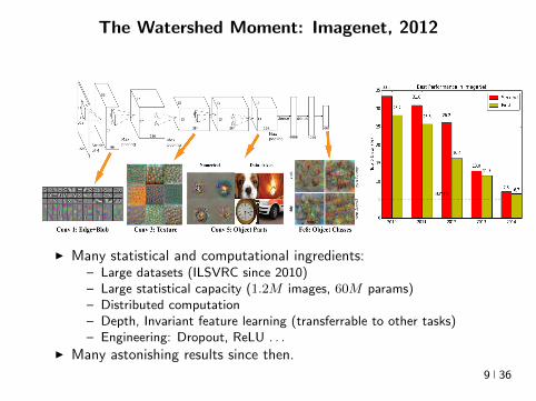
The Watershed Moment Imagenet 2012
I Many statistical and computational ingredientsndash Large datasets (ILSVRC since 2010)ndash Large statistical capacity (12M images 60M params)ndash Distributed computationndash Depth Invariant feature learning (transferrable to other tasks)ndash Engineering Dropout ReLU
I Many astonishing results since then
9 36
CNNs
10 36
Self-Driving Cars
Figure End-to-End Learning for Self-driving Cars Bojarski et al 2016
11 36

CNNs
10 36
Self-Driving Cars
Figure End-to-End Learning for Self-driving Cars Bojarski et al 2016
11 36

Self-Driving Cars
Figure End-to-End Learning for Self-driving Cars Bojarski et al 2016
11 36

Self-Driving Cars
Figure 72 hours 250K params 98perc autonomy
11 36
Self-Driving Cars
11 36

Self-Driving Cars
11 36

AlphaGo CNNs Deep-RL + Tree Search
I Tree complexity bd Chess (3580) Go (250150)
I Hard to evaluate a mid-position
I 19x19 board-img (48 planes) playeropponent 12-layer CNNs
I 30M human games 4 weeks 50 GPUs rarr 57 supervised learningrarr 80 RL [human-level]
D Silver et al Mastering the Game of Go with DNNs and Tree Search Nature 2016
12 36
Machine Learning in 1990s
I Convolutional Neural Networks (Fukushima 1980 Lecun et al 1989)
ndash 3 days to train on USPS (n = 7291 digit recognition) on SunSparcstation 1 (33MHz clock speed 64MB RAM)
I Personal history
ndash 1998 (Deep Blue Google Email) Train DNN on UCI Wine datasetndash 1999 Introduced to Kernel Methods - by DNN researchersndash 2003-4 NN paper at JMLR rejected accepted in IEEE Trans
Neural Nets with a kernel methods section
I Why Kernel Methods
ndash Local Minima free - stronger role of Convex Optimizationndash Theoretically appealingndash Handle non-vectorial data high-dimensional datandash Easier model selection via continuous optimizationndash Matched NN in many cases although didnt scale wrt n as well
I So what changed
ndash More data parallel algorithms hardware Better DNN training
13 36
Machine Learning in 1990s
I Convolutional Neural Networks (Fukushima 1980 Lecun et al 1989)
ndash 3 days to train on USPS (n = 7291 digit recognition) on SunSparcstation 1 (33MHz clock speed 64MB RAM)
I Personal history
ndash 1998 (Deep Blue Google Email) Train DNN on UCI Wine dataset
ndash 1999 Introduced to Kernel Methods - by DNN researchersndash 2003-4 NN paper at JMLR rejected accepted in IEEE Trans
Neural Nets with a kernel methods section
I Why Kernel Methods
ndash Local Minima free - stronger role of Convex Optimizationndash Theoretically appealingndash Handle non-vectorial data high-dimensional datandash Easier model selection via continuous optimizationndash Matched NN in many cases although didnt scale wrt n as well
I So what changed
ndash More data parallel algorithms hardware Better DNN training
13 36
Machine Learning in 1990s
I Convolutional Neural Networks (Fukushima 1980 Lecun et al 1989)
ndash 3 days to train on USPS (n = 7291 digit recognition) on SunSparcstation 1 (33MHz clock speed 64MB RAM)
I Personal history
ndash 1998 (Deep Blue Google Email) Train DNN on UCI Wine datasetndash 1999 Introduced to Kernel Methods - by DNN researchers
ndash 2003-4 NN paper at JMLR rejected accepted in IEEE TransNeural Nets with a kernel methods section
I Why Kernel Methods
ndash Local Minima free - stronger role of Convex Optimizationndash Theoretically appealingndash Handle non-vectorial data high-dimensional datandash Easier model selection via continuous optimizationndash Matched NN in many cases although didnt scale wrt n as well
I So what changed
ndash More data parallel algorithms hardware Better DNN training
13 36
Machine Learning in 1990s
I Convolutional Neural Networks (Fukushima 1980 Lecun et al 1989)
ndash 3 days to train on USPS (n = 7291 digit recognition) on SunSparcstation 1 (33MHz clock speed 64MB RAM)
I Personal history
ndash 1998 (Deep Blue Google Email) Train DNN on UCI Wine datasetndash 1999 Introduced to Kernel Methods - by DNN researchersndash 2003-4 NN paper at JMLR rejected accepted in IEEE Trans
Neural Nets with a kernel methods section
I Why Kernel Methods
ndash Local Minima free - stronger role of Convex Optimizationndash Theoretically appealingndash Handle non-vectorial data high-dimensional datandash Easier model selection via continuous optimizationndash Matched NN in many cases although didnt scale wrt n as well
I So what changed
ndash More data parallel algorithms hardware Better DNN training
13 36
Machine Learning in 1990s
I Convolutional Neural Networks (Fukushima 1980 Lecun et al 1989)
ndash 3 days to train on USPS (n = 7291 digit recognition) on SunSparcstation 1 (33MHz clock speed 64MB RAM)
I Personal history
ndash 1998 (Deep Blue Google Email) Train DNN on UCI Wine datasetndash 1999 Introduced to Kernel Methods - by DNN researchersndash 2003-4 NN paper at JMLR rejected accepted in IEEE Trans
Neural Nets with a kernel methods section
I Why Kernel Methods
ndash Local Minima free - stronger role of Convex Optimization
ndash Theoretically appealingndash Handle non-vectorial data high-dimensional datandash Easier model selection via continuous optimizationndash Matched NN in many cases although didnt scale wrt n as well
I So what changed
ndash More data parallel algorithms hardware Better DNN training
13 36
Machine Learning in 1990s
I Convolutional Neural Networks (Fukushima 1980 Lecun et al 1989)
ndash 3 days to train on USPS (n = 7291 digit recognition) on SunSparcstation 1 (33MHz clock speed 64MB RAM)
I Personal history
ndash 1998 (Deep Blue Google Email) Train DNN on UCI Wine datasetndash 1999 Introduced to Kernel Methods - by DNN researchersndash 2003-4 NN paper at JMLR rejected accepted in IEEE Trans
Neural Nets with a kernel methods section
I Why Kernel Methods
ndash Local Minima free - stronger role of Convex Optimizationndash Theoretically appealing
ndash Handle non-vectorial data high-dimensional datandash Easier model selection via continuous optimizationndash Matched NN in many cases although didnt scale wrt n as well
I So what changed
ndash More data parallel algorithms hardware Better DNN training
13 36
Machine Learning in 1990s
I Convolutional Neural Networks (Fukushima 1980 Lecun et al 1989)
ndash 3 days to train on USPS (n = 7291 digit recognition) on SunSparcstation 1 (33MHz clock speed 64MB RAM)
I Personal history
ndash 1998 (Deep Blue Google Email) Train DNN on UCI Wine datasetndash 1999 Introduced to Kernel Methods - by DNN researchersndash 2003-4 NN paper at JMLR rejected accepted in IEEE Trans
Neural Nets with a kernel methods section
I Why Kernel Methods
ndash Local Minima free - stronger role of Convex Optimizationndash Theoretically appealingndash Handle non-vectorial data high-dimensional datandash Easier model selection via continuous optimization
ndash Matched NN in many cases although didnt scale wrt n as well
I So what changed
ndash More data parallel algorithms hardware Better DNN training
13 36
Machine Learning in 1990s
I Convolutional Neural Networks (Fukushima 1980 Lecun et al 1989)
ndash 3 days to train on USPS (n = 7291 digit recognition) on SunSparcstation 1 (33MHz clock speed 64MB RAM)
I Personal history
ndash 1998 (Deep Blue Google Email) Train DNN on UCI Wine datasetndash 1999 Introduced to Kernel Methods - by DNN researchersndash 2003-4 NN paper at JMLR rejected accepted in IEEE Trans
Neural Nets with a kernel methods section
I Why Kernel Methods
ndash Local Minima free - stronger role of Convex Optimizationndash Theoretically appealingndash Handle non-vectorial data high-dimensional datandash Easier model selection via continuous optimizationndash Matched NN in many cases although didnt scale wrt n as well
I So what changed
ndash More data parallel algorithms hardware Better DNN training
13 36
Machine Learning in 1990s
I Convolutional Neural Networks (Fukushima 1980 Lecun et al 1989)
ndash 3 days to train on USPS (n = 7291 digit recognition) on SunSparcstation 1 (33MHz clock speed 64MB RAM)
I Personal history
ndash 1998 (Deep Blue Google Email) Train DNN on UCI Wine datasetndash 1999 Introduced to Kernel Methods - by DNN researchersndash 2003-4 NN paper at JMLR rejected accepted in IEEE Trans
Neural Nets with a kernel methods section
I Why Kernel Methods
ndash Local Minima free - stronger role of Convex Optimizationndash Theoretically appealingndash Handle non-vectorial data high-dimensional datandash Easier model selection via continuous optimizationndash Matched NN in many cases although didnt scale wrt n as well
I So what changed
ndash More data parallel algorithms hardware Better DNN training
13 36
Kernel Methods vs Neural Networks (Pre-Google)
14 36
Kernel Methods vs Neural Networks
Geoff Hinton facts meme maintained athttpyannlecuncomexfun
I All kernels that ever dared approaching Geoff Hinton woke upconvolved
I The only kernel Geoff Hinton has ever used is a kernel of truth
I If you defy Geoff Hinton he will maximize your entropy in no timeYour free energy will be gone even before you reach equilibrium
Are there synergies between these fields towards design of even better(faster and more accurate) algorithms
15 36
Linear Hypotheses
I f(x) = wTxw isin Rn Assume Y sub R setting
arg minwisinRd
lsumi=1
(yi minuswTxi)2 + λw22
w = (XTX + λId)minus1 (XTy
)X =
xTi
isin Rltimesn
I ntimes n linear system =rArr O(ln2 + n3) training time assuming nostructure (eg sparsity)
I O(n) prediction time
I High Approximation error
16 36
Polynomials The expensive way
I Homogeneous degree-d polynomial
f(x) = wTΨnd(x) w isin Rs s =
(d+ nminus 1
d
)
Ψnd(x) =
radic(dα
)xα
isin Rs
α = (α1 αn)sumi
αi = d
(d
α
)=
d
α1 αn
xα = xα11 xα2
2 xαnn
I Construct Z isin Rntimess with rows Ψnd(xi) and solve in O(s3) () time
w = (ZTZ + λId)minus1 (ZTy) (1)
I Note n = 100 d = 4 =rArr s gt 4M
17 36
Polynomials
I Consider the subspace of Rs spanned by the data
S = span (Ψ(x1) Ψ(xl)) = v isin Rs v =
lsumi=1
αiΨ(xi)
I So Rs = S + Sperp Hence for any vector w isin Rs
w = wS + wSperp
I The search of a minimizer can be reduced to S because
lsumi=1
V (wTΨ(xi)) + λw22 gelsumi=1
V (wTSΨ(xi)) + λwS22 + wperpS 22
gelsumi=1
V (wTSΨ(xi)) + λwS22 (2)
I Argument holds for any loss (convex or non-convex additive or not)but needs orthogonality (l2 regularizer) [Representer Theorem]
18 36
Polynomials
I Hence w =sumli=1 βiΨ(xi) isin S for β isin Rl and so we can solve
arg minwisinRd
lsumi=1
(yi minuswTΨ(xi))2 + λw22
arg minβisinRl
lsumj=1
(yj minus
lsumi=1
βiΨ(xi)TΨ(xj)
)2
+ λ
lsumij=1
βiβjΨ(xi)TΨ(xj)
arg minβisinRl
lsumj=1
(yj minus (Gβ)j
)2+ λβTGβ
Gij = Ψ(xi)TΨ(xj)
β = (G + λId)minus1
y
I O(l3 + sl2) training time - O(s3) cost eliminatedI Inference time (O(s) or O(ls))
f(x) = wTΨ(x) =
lsumi=1
βiΨ(xi)TΨ(x)
19 36
Polynomials
I Multinomial Theorem
(z1 + z2 + + zn)d =sum
α|α|=d
(d
α
)zα
I Implicit computation of inner products
Ψ(x)TΨ(xprime) =
ssumi=1
(d
α
)xαxprime
α=
ssumi=1
(d
α
)xα11 xαnn x
primeα11 x
primeαnn
=
ssumi=1
(d
α
)(x1x
prime1)α1(x2x
prime2)α2 (xnx
primen)αn
= (x1xprime1 + xnx
primen)d
= (xTxprime)d
I O(l3 + l2n) training and O(ln) predicting speedI Complexity coming from s has been completely eliminated ()
[Kernel Trick]
20 36
Polynomials Algorithm
I Algorithm
ndash Start with k X times X 7rarr R k(xxprime) = (xTxprime + 1)d
ndash Construct Gram matrix Gij = k(xixj) on the training samplesndash Solve β = (G + λId)minus1 yndash Return f(x) =
sumli=1 βik(xix)
I f is the optimal degree-d polynomial solving the learning problemin complexity independent of d
I What other forms of k correspond to linear learning inhigh-dimensional nonlinear embeddings of the data
21 36
Symmetric positive semi-definite functions
I Definition A function k X times X 7rarr R is psd if for any finitecollection of points x1 xl the l times l Gram matrix
Gij = k(xixj)
is positive semi-definite ie for any vector β isin Rl
βTGβ =sumij
βiβjk(xixj) ge 0
I Theorem[Mercer] If k is symmetric psd X is compact subset ofRn then it admits an eigenfunction decomposition
k(xxprime) =
Nsumi=1
λiφj(x)φj(xprime) = 〈Ψ(x)Ψ(xprime)〉l2
Ψ(x) = [ radicλjφ(x) ]T (3)
I Feature map associated with a kernel is not uniqueI Functional generalization of positive semi-definite matrices
22 36
Kernels
I Lineark(xxprime) = xTxprime
I Polynomialk(xxprime) = (xTxprime + 1)d
I Gaussian s =infin Universal
k(xxprime) = eminusxminusxprime2
2σ2
I Conic combinations
k(xxprime) = α1k1(xxprime) + α2k2(xxprime)
I Elementwise products
k(xxprime) = k1(xxprime)k2(xxprime)
I Kernels on discrete sets strings graphs sequences shapes
23 36
Gaussian Kernel is Positive Definite
I Exponential
eβxTxprime = 1 + βxTxprime +
β2
2(xTy)2 +
β3
3(xTy)3 +
I For any function f Rn 7rarr R psd function k the following kernelis psd
kprime(xxprime) = f(x) (k(xxprime)) f(xprime)
Proofsumij
βiβjkprime(xixj) =
sumij
βiβjf(xi)k(xixj)f(xj) =sumij
βprimeiβprimejk(xixj) ge 0
I Gaussian Kernel
k(xxprime) = eminusxminusxprime22
2σ2
= eminusx222σ2
(e
2xT xprime2σ2
)eminusxprime222σ2 (4)
24 36
The Mathematical Naturalness of Kernel Methods
I Data X isin Rd Models isin H X 7rarr R
I Geometry in H inner product 〈middot middot〉H norm middot H (Hilbert Spaces)I Theorem All nice Hilbert spaces are generated by a symmetric
positive definite function (the kernel) k(xxprime) on X times XI if f g isin H close ie f minus gH small then f(x) g(x) close forallx isin X I Reproducing Kernel Hilbert Spaces (RKHSs) Hilbert space H
that admit a reproducing kernel ie a function k(xxprime) satisfying
(i) forallx isin X k(middotx) isin H(ii) 〈f k(middotx)〉H = f(x)
I Reproducing kernels are symmetric psdsumij
βiβjk(xixj) = 〈sumi
βik(middotxi)sumi
βik(middotxi)〉H
= sumi
βik(middotxi)2H ge 0 (5)
I (Moore-Aronsjan 1950) Symmetric psd functions arereproducing kernels for some (unique) RKHS Hk
25 36
The Mathematical Naturalness of Kernel Methods
I Data X isin Rd Models isin H X 7rarr RI Geometry in H inner product 〈middot middot〉H norm middot H (Hilbert Spaces)
I Theorem All nice Hilbert spaces are generated by a symmetricpositive definite function (the kernel) k(xxprime) on X times X
I if f g isin H close ie f minus gH small then f(x) g(x) close forallx isin X I Reproducing Kernel Hilbert Spaces (RKHSs) Hilbert space H
that admit a reproducing kernel ie a function k(xxprime) satisfying
(i) forallx isin X k(middotx) isin H(ii) 〈f k(middotx)〉H = f(x)
I Reproducing kernels are symmetric psdsumij
βiβjk(xixj) = 〈sumi
βik(middotxi)sumi
βik(middotxi)〉H
= sumi
βik(middotxi)2H ge 0 (5)
I (Moore-Aronsjan 1950) Symmetric psd functions arereproducing kernels for some (unique) RKHS Hk
25 36
The Mathematical Naturalness of Kernel Methods
I Data X isin Rd Models isin H X 7rarr RI Geometry in H inner product 〈middot middot〉H norm middot H (Hilbert Spaces)I Theorem All nice Hilbert spaces are generated by a symmetric
positive definite function (the kernel) k(xxprime) on X times XI if f g isin H close ie f minus gH small then f(x) g(x) close forallx isin X
I Reproducing Kernel Hilbert Spaces (RKHSs) Hilbert space Hthat admit a reproducing kernel ie a function k(xxprime) satisfying
(i) forallx isin X k(middotx) isin H(ii) 〈f k(middotx)〉H = f(x)
I Reproducing kernels are symmetric psdsumij
βiβjk(xixj) = 〈sumi
βik(middotxi)sumi
βik(middotxi)〉H
= sumi
βik(middotxi)2H ge 0 (5)
I (Moore-Aronsjan 1950) Symmetric psd functions arereproducing kernels for some (unique) RKHS Hk
25 36
The Mathematical Naturalness of Kernel Methods
I Data X isin Rd Models isin H X 7rarr RI Geometry in H inner product 〈middot middot〉H norm middot H (Hilbert Spaces)I Theorem All nice Hilbert spaces are generated by a symmetric
positive definite function (the kernel) k(xxprime) on X times XI if f g isin H close ie f minus gH small then f(x) g(x) close forallx isin X I Reproducing Kernel Hilbert Spaces (RKHSs) Hilbert space H
that admit a reproducing kernel ie a function k(xxprime) satisfying
(i) forallx isin X k(middotx) isin H(ii) 〈f k(middotx)〉H = f(x)
I Reproducing kernels are symmetric psdsumij
βiβjk(xixj) = 〈sumi
βik(middotxi)sumi
βik(middotxi)〉H
= sumi
βik(middotxi)2H ge 0 (5)
I (Moore-Aronsjan 1950) Symmetric psd functions arereproducing kernels for some (unique) RKHS Hk
25 36
The Mathematical Naturalness of Kernel Methods
I Data X isin Rd Models isin H X 7rarr RI Geometry in H inner product 〈middot middot〉H norm middot H (Hilbert Spaces)I Theorem All nice Hilbert spaces are generated by a symmetric
positive definite function (the kernel) k(xxprime) on X times XI if f g isin H close ie f minus gH small then f(x) g(x) close forallx isin X I Reproducing Kernel Hilbert Spaces (RKHSs) Hilbert space H
that admit a reproducing kernel ie a function k(xxprime) satisfying
(i) forallx isin X k(middotx) isin H(ii) 〈f k(middotx)〉H = f(x)
I Reproducing kernels are symmetric psdsumij
βiβjk(xixj) = 〈sumi
βik(middotxi)sumi
βik(middotxi)〉H
= sumi
βik(middotxi)2H ge 0 (5)
I (Moore-Aronsjan 1950) Symmetric psd functions arereproducing kernels for some (unique) RKHS Hk 25 36
Kernel Methods Summary
I Symm pos def function k(x z) on input domain X sub Rd
I k hArr rich Reproducing Kernel Hilbert Space (RKHS) Hk ofreal-valued functions with inner product 〈middot middot〉k and norm middot k
I Regularized Risk Minimization hArr Linear models in an implicithigh-dimensional (often infinite-dimensional) feature space
f = arg minfisinHk
1
n
nsumi=1
V (yi f(xi)) + λf2Hk xi isin Rd
I Representer Theorem f(x) =sumni=1 αik(xxi)
26 36
Shallow and Deep Function Spaces
I What does it mean to understand a function space
ndash Linear f(x) = wTxw isin Rd
ndash Polynomial f(x) = wT Ψ(x)w isin Rs
ndash RKHS balls f isin Hk fk lt γ [like vM le 1]
I Shallow nets f(x) = wTσ(Wx) (w isin RdW isin Rs)ndash For srarrinfin W sim p σ(u) = eminusiu approximates Gaussian kernel
methodsndash Theorem [Bochner 1937] One-to-one correspondence between k
and a density p such that
k(x z) = ψ(xminus z) =
intRdeminusi(xminusz)Twp(w)dw asymp 1
s
ssumj=1
eminusi(xminusz)Twj
Gaussian kernel k(x z) = eminusxminusz22
2σ2 lArrrArr p = N (0 σminus2Id)ndash Similar integral approx relates ReLU to the arc-cosine kernelndash Optimization versus Randomization
27 36
Shallow and Deep Function Spaces
I What does it mean to understand a function space
ndash Linear f(x) = wTxw isin Rd
ndash Polynomial f(x) = wT Ψ(x)w isin Rs
ndash RKHS balls f isin Hk fk lt γ [like vM le 1]
I Shallow nets f(x) = wTσ(Wx) (w isin RdW isin Rs)
ndash For srarrinfin W sim p σ(u) = eminusiu approximates Gaussian kernelmethods
ndash Theorem [Bochner 1937] One-to-one correspondence between kand a density p such that
k(x z) = ψ(xminus z) =
intRdeminusi(xminusz)Twp(w)dw asymp 1
s
ssumj=1
eminusi(xminusz)Twj
Gaussian kernel k(x z) = eminusxminusz22
2σ2 lArrrArr p = N (0 σminus2Id)ndash Similar integral approx relates ReLU to the arc-cosine kernelndash Optimization versus Randomization
27 36
Shallow and Deep Function Spaces
I What does it mean to understand a function space
ndash Linear f(x) = wTxw isin Rd
ndash Polynomial f(x) = wT Ψ(x)w isin Rs
ndash RKHS balls f isin Hk fk lt γ [like vM le 1]
I Shallow nets f(x) = wTσ(Wx) (w isin RdW isin Rs)ndash For srarrinfin W sim p σ(u) = eminusiu approximates Gaussian kernel
methodsndash Theorem [Bochner 1937] One-to-one correspondence between k
and a density p such that
k(x z) = ψ(xminus z) =
intRdeminusi(xminusz)Twp(w)dw asymp 1
s
ssumj=1
eminusi(xminusz)Twj
Gaussian kernel k(x z) = eminusxminusz22
2σ2 lArrrArr p = N (0 σminus2Id)ndash Similar integral approx relates ReLU to the arc-cosine kernelndash Optimization versus Randomization
27 36
Expressivity of Deep Nets Linear Regions
I The ReLU map f(x) = max(Wx 0)W isin Rwtimesn is piecewise linear
I A piece is a connected region (a convex polytope) of Rd with sharedsparsity pattern in activations
I (Zaslavsky 1975) Number of linear regions formed by an arrangement of
s hyperplanes in d-dimensions in general position issumd
i=0
(si
)I Composition of ReLU maps is also piecewise linear
I (Raghu et al 2017 Pascano et al 2014 Montufar 2014) Number oflinear regions grows as O(wnd) for a composition of d ReLU maps(nrarr brarr brarr b rarr b) each of width w
I (Safran and Shamir 2017)
ndash 1[x le 1] x isin Rd ε-accurate 3-layer network with O(dε) neurons but cannot be approximated with
accuracy higher than O(1d4) using 2-layer networks unless width is exponential in d
28 36
Expressivity of Deep Nets Linear Regions
I The ReLU map f(x) = max(Wx 0)W isin Rwtimesn is piecewise linear
I A piece is a connected region (a convex polytope) of Rd with sharedsparsity pattern in activations
I (Zaslavsky 1975) Number of linear regions formed by an arrangement of
s hyperplanes in d-dimensions in general position issumd
i=0
(si
)
I Composition of ReLU maps is also piecewise linear
I (Raghu et al 2017 Pascano et al 2014 Montufar 2014) Number oflinear regions grows as O(wnd) for a composition of d ReLU maps(nrarr brarr brarr b rarr b) each of width w
I (Safran and Shamir 2017)
ndash 1[x le 1] x isin Rd ε-accurate 3-layer network with O(dε) neurons but cannot be approximated with
accuracy higher than O(1d4) using 2-layer networks unless width is exponential in d
28 36
Expressivity of Deep Nets Linear Regions
I The ReLU map f(x) = max(Wx 0)W isin Rwtimesn is piecewise linear
I A piece is a connected region (a convex polytope) of Rd with sharedsparsity pattern in activations
I (Zaslavsky 1975) Number of linear regions formed by an arrangement of
s hyperplanes in d-dimensions in general position issumd
i=0
(si
)I Composition of ReLU maps is also piecewise linear
I (Raghu et al 2017 Pascano et al 2014 Montufar 2014) Number oflinear regions grows as O(wnd) for a composition of d ReLU maps(nrarr brarr brarr b rarr b) each of width w
I (Safran and Shamir 2017)
ndash 1[x le 1] x isin Rd ε-accurate 3-layer network with O(dε) neurons but cannot be approximated with
accuracy higher than O(1d4) using 2-layer networks unless width is exponential in d28 36
Expressivity of Deep Nets Trajectory Length
I (Raghu et al 2017) Trajectory Length (ldquogeneralized operator normrdquo)How much is a curve in the input space stretched by a layer in thenetwork
29 36
Expressivity of Deep Nets Trajectory Length
I (Raghu et al 2017) Trajectory Length (ldquogeneralized operator normrdquo)How much is a curve in the input space stretched by a layer in thenetwork
29 36
Expressivity and Generalization
I Expressiveness equiv capacity to fit random noise =rArr susceptibility tooverfitting (VC dimension Rademacher Complexity)
I Zhang et al 2017 Famous CNNs easily fit random labels
ndash Over-parameterized (n=12M psim 60M) but structuredndash Domain-knowledge baked in does not constraint expressiveness
I CNNs tend to generalize even without regularization (explicit and implicit)
I For linear regression SGD returns minimum norm solution
30 36
Optimization Landscape Symmetry and Saddle Points
I Folklore lots of equivalent good local minI Classification of critical points based on Hessian spectrumI Permutation and Scaling symmetries
I Thm [Lee et al 2016 Anadkumar Ge] For the short-step gradientmethod the basin of attraction of strict saddle points (atleast onenegative eigenvalue) has measure zero
31 36
Optimization Landscape Sharp Minima and Stability
Keskar et al 2017 On large-batch training for DL Generalization Gap and Sharp Minima
32 36
Deep Learning Computational Graphs TensorFlow
tensorfloworg
I Tensors-in Tensors-out
I Evergrowing list of Tensor-Ops (PythonC++)
f(xw)
[partf
partx
]T v
[partf
partw
]T v
I Automatic Differentiation Reverse mode
partxL
partxi=sumirarrj
partxL
partxj
partxj
partxi
33 36
Computational Graphs and TensorFlow
tensorfloworg
I SGD with minibatches
wk+1 = wk minus ηlsumi=1
partli
partw
∣∣∣wt
I Model Parallelism Assign independent paths tothreads GPUs
I Data Parallelism create Graph replicas on differentmachines
I Mobile TensorFlow
34 36
Computational Graphs and TensorFlow
tensorfloworg
35 36
Computational Graphs and TensorFlow
tensorfloworg
35 36
Computational Graphs and TensorFlow
tensorfloworg
35 36
Challenges and Opportunities
I Lots of fascinating unsolved problems
I Can you win Imagenet with Convex optimization
I Tools from polynomial optimization (global optimization deep-RL)
I Supervised to Semi-supervised to Unsupervised Learning
I Compact efficient real-time models (eliminateover-parametrization) for new form factors
I Exciting emerging world of Robotics Wearable ComputersIntelligent home devices Personal digital assistants
Google Internship Program
36 36
- anm0
- fdrm0
- fdrm5

AlphaGo CNNs Deep-RL + Tree Search
I Tree complexity bd Chess (3580) Go (250150)
I Hard to evaluate a mid-position
I 19x19 board-img (48 planes) playeropponent 12-layer CNNs
I 30M human games 4 weeks 50 GPUs rarr 57 supervised learningrarr 80 RL [human-level]
D Silver et al Mastering the Game of Go with DNNs and Tree Search Nature 2016
12 36
Machine Learning in 1990s
I Convolutional Neural Networks (Fukushima 1980 Lecun et al 1989)
ndash 3 days to train on USPS (n = 7291 digit recognition) on SunSparcstation 1 (33MHz clock speed 64MB RAM)
I Personal history
ndash 1998 (Deep Blue Google Email) Train DNN on UCI Wine datasetndash 1999 Introduced to Kernel Methods - by DNN researchersndash 2003-4 NN paper at JMLR rejected accepted in IEEE Trans
Neural Nets with a kernel methods section
I Why Kernel Methods
ndash Local Minima free - stronger role of Convex Optimizationndash Theoretically appealingndash Handle non-vectorial data high-dimensional datandash Easier model selection via continuous optimizationndash Matched NN in many cases although didnt scale wrt n as well
I So what changed
ndash More data parallel algorithms hardware Better DNN training
13 36
Machine Learning in 1990s
I Convolutional Neural Networks (Fukushima 1980 Lecun et al 1989)
ndash 3 days to train on USPS (n = 7291 digit recognition) on SunSparcstation 1 (33MHz clock speed 64MB RAM)
I Personal history
ndash 1998 (Deep Blue Google Email) Train DNN on UCI Wine dataset
ndash 1999 Introduced to Kernel Methods - by DNN researchersndash 2003-4 NN paper at JMLR rejected accepted in IEEE Trans
Neural Nets with a kernel methods section
I Why Kernel Methods
ndash Local Minima free - stronger role of Convex Optimizationndash Theoretically appealingndash Handle non-vectorial data high-dimensional datandash Easier model selection via continuous optimizationndash Matched NN in many cases although didnt scale wrt n as well
I So what changed
ndash More data parallel algorithms hardware Better DNN training
13 36
Machine Learning in 1990s
I Convolutional Neural Networks (Fukushima 1980 Lecun et al 1989)
ndash 3 days to train on USPS (n = 7291 digit recognition) on SunSparcstation 1 (33MHz clock speed 64MB RAM)
I Personal history
ndash 1998 (Deep Blue Google Email) Train DNN on UCI Wine datasetndash 1999 Introduced to Kernel Methods - by DNN researchers
ndash 2003-4 NN paper at JMLR rejected accepted in IEEE TransNeural Nets with a kernel methods section
I Why Kernel Methods
ndash Local Minima free - stronger role of Convex Optimizationndash Theoretically appealingndash Handle non-vectorial data high-dimensional datandash Easier model selection via continuous optimizationndash Matched NN in many cases although didnt scale wrt n as well
I So what changed
ndash More data parallel algorithms hardware Better DNN training
13 36
Machine Learning in 1990s
I Convolutional Neural Networks (Fukushima 1980 Lecun et al 1989)
ndash 3 days to train on USPS (n = 7291 digit recognition) on SunSparcstation 1 (33MHz clock speed 64MB RAM)
I Personal history
ndash 1998 (Deep Blue Google Email) Train DNN on UCI Wine datasetndash 1999 Introduced to Kernel Methods - by DNN researchersndash 2003-4 NN paper at JMLR rejected accepted in IEEE Trans
Neural Nets with a kernel methods section
I Why Kernel Methods
ndash Local Minima free - stronger role of Convex Optimizationndash Theoretically appealingndash Handle non-vectorial data high-dimensional datandash Easier model selection via continuous optimizationndash Matched NN in many cases although didnt scale wrt n as well
I So what changed
ndash More data parallel algorithms hardware Better DNN training
13 36
Machine Learning in 1990s
I Convolutional Neural Networks (Fukushima 1980 Lecun et al 1989)
ndash 3 days to train on USPS (n = 7291 digit recognition) on SunSparcstation 1 (33MHz clock speed 64MB RAM)
I Personal history
ndash 1998 (Deep Blue Google Email) Train DNN on UCI Wine datasetndash 1999 Introduced to Kernel Methods - by DNN researchersndash 2003-4 NN paper at JMLR rejected accepted in IEEE Trans
Neural Nets with a kernel methods section
I Why Kernel Methods
ndash Local Minima free - stronger role of Convex Optimizationndash Theoretically appealingndash Handle non-vectorial data high-dimensional datandash Easier model selection via continuous optimizationndash Matched NN in many cases although didnt scale wrt n as well
I So what changed
ndash More data parallel algorithms hardware Better DNN training
13 36
Machine Learning in 1990s
I Convolutional Neural Networks (Fukushima 1980 Lecun et al 1989)
ndash 3 days to train on USPS (n = 7291 digit recognition) on SunSparcstation 1 (33MHz clock speed 64MB RAM)
I Personal history
ndash 1998 (Deep Blue Google Email) Train DNN on UCI Wine datasetndash 1999 Introduced to Kernel Methods - by DNN researchersndash 2003-4 NN paper at JMLR rejected accepted in IEEE Trans
Neural Nets with a kernel methods section
I Why Kernel Methods
ndash Local Minima free - stronger role of Convex Optimization
ndash Theoretically appealingndash Handle non-vectorial data high-dimensional datandash Easier model selection via continuous optimizationndash Matched NN in many cases although didnt scale wrt n as well
I So what changed
ndash More data parallel algorithms hardware Better DNN training
13 36
Machine Learning in 1990s
I Convolutional Neural Networks (Fukushima 1980 Lecun et al 1989)
ndash 3 days to train on USPS (n = 7291 digit recognition) on SunSparcstation 1 (33MHz clock speed 64MB RAM)
I Personal history
ndash 1998 (Deep Blue Google Email) Train DNN on UCI Wine datasetndash 1999 Introduced to Kernel Methods - by DNN researchersndash 2003-4 NN paper at JMLR rejected accepted in IEEE Trans
Neural Nets with a kernel methods section
I Why Kernel Methods
ndash Local Minima free - stronger role of Convex Optimizationndash Theoretically appealing
ndash Handle non-vectorial data high-dimensional datandash Easier model selection via continuous optimizationndash Matched NN in many cases although didnt scale wrt n as well
I So what changed
ndash More data parallel algorithms hardware Better DNN training
13 36
Machine Learning in 1990s
I Convolutional Neural Networks (Fukushima 1980 Lecun et al 1989)
ndash 3 days to train on USPS (n = 7291 digit recognition) on SunSparcstation 1 (33MHz clock speed 64MB RAM)
I Personal history
ndash 1998 (Deep Blue Google Email) Train DNN on UCI Wine datasetndash 1999 Introduced to Kernel Methods - by DNN researchersndash 2003-4 NN paper at JMLR rejected accepted in IEEE Trans
Neural Nets with a kernel methods section
I Why Kernel Methods
ndash Local Minima free - stronger role of Convex Optimizationndash Theoretically appealingndash Handle non-vectorial data high-dimensional datandash Easier model selection via continuous optimization
ndash Matched NN in many cases although didnt scale wrt n as well
I So what changed
ndash More data parallel algorithms hardware Better DNN training
13 36
Machine Learning in 1990s
I Convolutional Neural Networks (Fukushima 1980 Lecun et al 1989)
ndash 3 days to train on USPS (n = 7291 digit recognition) on SunSparcstation 1 (33MHz clock speed 64MB RAM)
I Personal history
ndash 1998 (Deep Blue Google Email) Train DNN on UCI Wine datasetndash 1999 Introduced to Kernel Methods - by DNN researchersndash 2003-4 NN paper at JMLR rejected accepted in IEEE Trans
Neural Nets with a kernel methods section
I Why Kernel Methods
ndash Local Minima free - stronger role of Convex Optimizationndash Theoretically appealingndash Handle non-vectorial data high-dimensional datandash Easier model selection via continuous optimizationndash Matched NN in many cases although didnt scale wrt n as well
I So what changed
ndash More data parallel algorithms hardware Better DNN training
13 36
Machine Learning in 1990s
I Convolutional Neural Networks (Fukushima 1980 Lecun et al 1989)
ndash 3 days to train on USPS (n = 7291 digit recognition) on SunSparcstation 1 (33MHz clock speed 64MB RAM)
I Personal history
ndash 1998 (Deep Blue Google Email) Train DNN on UCI Wine datasetndash 1999 Introduced to Kernel Methods - by DNN researchersndash 2003-4 NN paper at JMLR rejected accepted in IEEE Trans
Neural Nets with a kernel methods section
I Why Kernel Methods
ndash Local Minima free - stronger role of Convex Optimizationndash Theoretically appealingndash Handle non-vectorial data high-dimensional datandash Easier model selection via continuous optimizationndash Matched NN in many cases although didnt scale wrt n as well
I So what changed
ndash More data parallel algorithms hardware Better DNN training
13 36
Kernel Methods vs Neural Networks (Pre-Google)
14 36
Kernel Methods vs Neural Networks
Geoff Hinton facts meme maintained athttpyannlecuncomexfun
I All kernels that ever dared approaching Geoff Hinton woke upconvolved
I The only kernel Geoff Hinton has ever used is a kernel of truth
I If you defy Geoff Hinton he will maximize your entropy in no timeYour free energy will be gone even before you reach equilibrium
Are there synergies between these fields towards design of even better(faster and more accurate) algorithms
15 36
Kernel Methods vs Neural Networks
Geoff Hinton facts meme maintained athttpyannlecuncomexfun
I All kernels that ever dared approaching Geoff Hinton woke upconvolved
I The only kernel Geoff Hinton has ever used is a kernel of truth
I If you defy Geoff Hinton he will maximize your entropy in no timeYour free energy will be gone even before you reach equilibrium
Are there synergies between these fields towards design of even better(faster and more accurate) algorithms
15 36
Kernel Methods vs Neural Networks
Geoff Hinton facts meme maintained athttpyannlecuncomexfun
I All kernels that ever dared approaching Geoff Hinton woke upconvolved
I The only kernel Geoff Hinton has ever used is a kernel of truth
I If you defy Geoff Hinton he will maximize your entropy in no timeYour free energy will be gone even before you reach equilibrium
Are there synergies between these fields towards design of even better(faster and more accurate) algorithms
15 36
Linear Hypotheses
I f(x) = wTxw isin Rn Assume Y sub R setting
arg minwisinRd
lsumi=1
(yi minuswTxi)2 + λw22
w = (XTX + λId)minus1 (XTy
)X =
xTi
isin Rltimesn
I ntimes n linear system =rArr O(ln2 + n3) training time assuming nostructure (eg sparsity)
I O(n) prediction time
I High Approximation error
16 36
Polynomials The expensive way
I Homogeneous degree-d polynomial
f(x) = wTΨnd(x) w isin Rs s =
(d+ nminus 1
d
)
Ψnd(x) =
radic(dα
)xα
isin Rs
α = (α1 αn)sumi
αi = d
(d
α
)=
d
α1 αn
xα = xα11 xα2
2 xαnn
I Construct Z isin Rntimess with rows Ψnd(xi) and solve in O(s3) () time
w = (ZTZ + λId)minus1 (ZTy) (1)
I Note n = 100 d = 4 =rArr s gt 4M
17 36
Polynomials
I Consider the subspace of Rs spanned by the data
S = span (Ψ(x1) Ψ(xl)) = v isin Rs v =
lsumi=1
αiΨ(xi)
I So Rs = S + Sperp Hence for any vector w isin Rs
w = wS + wSperp
I The search of a minimizer can be reduced to S because
lsumi=1
V (wTΨ(xi)) + λw22 gelsumi=1
V (wTSΨ(xi)) + λwS22 + wperpS 22
gelsumi=1
V (wTSΨ(xi)) + λwS22 (2)
I Argument holds for any loss (convex or non-convex additive or not)but needs orthogonality (l2 regularizer) [Representer Theorem]
18 36
Polynomials
I Consider the subspace of Rs spanned by the data
S = span (Ψ(x1) Ψ(xl)) = v isin Rs v =
lsumi=1
αiΨ(xi)
I So Rs = S + Sperp Hence for any vector w isin Rs
w = wS + wSperp
I The search of a minimizer can be reduced to S because
lsumi=1
V (wTΨ(xi)) + λw22 gelsumi=1
V (wTSΨ(xi)) + λwS22 + wperpS 22
gelsumi=1
V (wTSΨ(xi)) + λwS22 (2)
I Argument holds for any loss (convex or non-convex additive or not)but needs orthogonality (l2 regularizer) [Representer Theorem]
18 36
Polynomials
I Consider the subspace of Rs spanned by the data
S = span (Ψ(x1) Ψ(xl)) = v isin Rs v =
lsumi=1
αiΨ(xi)
I So Rs = S + Sperp Hence for any vector w isin Rs
w = wS + wSperp
I The search of a minimizer can be reduced to S because
lsumi=1
V (wTΨ(xi)) + λw22 gelsumi=1
V (wTSΨ(xi)) + λwS22 + wperpS 22
gelsumi=1
V (wTSΨ(xi)) + λwS22 (2)
I Argument holds for any loss (convex or non-convex additive or not)but needs orthogonality (l2 regularizer) [Representer Theorem]
18 36
Polynomials
I Consider the subspace of Rs spanned by the data
S = span (Ψ(x1) Ψ(xl)) = v isin Rs v =
lsumi=1
αiΨ(xi)
I So Rs = S + Sperp Hence for any vector w isin Rs
w = wS + wSperp
I The search of a minimizer can be reduced to S because
lsumi=1
V (wTΨ(xi)) + λw22 gelsumi=1
V (wTSΨ(xi)) + λwS22 + wperpS 22
gelsumi=1
V (wTSΨ(xi)) + λwS22 (2)
I Argument holds for any loss (convex or non-convex additive or not)but needs orthogonality (l2 regularizer) [Representer Theorem]
18 36
Polynomials
I Hence w =sumli=1 βiΨ(xi) isin S for β isin Rl and so we can solve
arg minwisinRd
lsumi=1
(yi minuswTΨ(xi))2 + λw22
arg minβisinRl
lsumj=1
(yj minus
lsumi=1
βiΨ(xi)TΨ(xj)
)2
+ λ
lsumij=1
βiβjΨ(xi)TΨ(xj)
arg minβisinRl
lsumj=1
(yj minus (Gβ)j
)2+ λβTGβ
Gij = Ψ(xi)TΨ(xj)
β = (G + λId)minus1
y
I O(l3 + sl2) training time - O(s3) cost eliminatedI Inference time (O(s) or O(ls))
f(x) = wTΨ(x) =
lsumi=1
βiΨ(xi)TΨ(x)
19 36
Polynomials
I Hence w =sumli=1 βiΨ(xi) isin S for β isin Rl and so we can solve
arg minwisinRd
lsumi=1
(yi minuswTΨ(xi))2 + λw22
arg minβisinRl
lsumj=1
(yj minus
lsumi=1
βiΨ(xi)TΨ(xj)
)2
+ λ
lsumij=1
βiβjΨ(xi)TΨ(xj)
arg minβisinRl
lsumj=1
(yj minus (Gβ)j
)2+ λβTGβ
Gij = Ψ(xi)TΨ(xj)
β = (G + λId)minus1
y
I O(l3 + sl2) training time - O(s3) cost eliminatedI Inference time (O(s) or O(ls))
f(x) = wTΨ(x) =
lsumi=1
βiΨ(xi)TΨ(x)
19 36
Polynomials
I Hence w =sumli=1 βiΨ(xi) isin S for β isin Rl and so we can solve
arg minwisinRd
lsumi=1
(yi minuswTΨ(xi))2 + λw22
arg minβisinRl
lsumj=1
(yj minus
lsumi=1
βiΨ(xi)TΨ(xj)
)2
+ λ
lsumij=1
βiβjΨ(xi)TΨ(xj)
arg minβisinRl
lsumj=1
(yj minus (Gβ)j
)2+ λβTGβ
Gij = Ψ(xi)TΨ(xj)
β = (G + λId)minus1
y
I O(l3 + sl2) training time - O(s3) cost eliminatedI Inference time (O(s) or O(ls))
f(x) = wTΨ(x) =
lsumi=1
βiΨ(xi)TΨ(x)
19 36
Polynomials
I Multinomial Theorem
(z1 + z2 + + zn)d =sum
α|α|=d
(d
α
)zα
I Implicit computation of inner products
Ψ(x)TΨ(xprime) =
ssumi=1
(d
α
)xαxprime
α=
ssumi=1
(d
α
)xα11 xαnn x
primeα11 x
primeαnn
=
ssumi=1
(d
α
)(x1x
prime1)α1(x2x
prime2)α2 (xnx
primen)αn
= (x1xprime1 + xnx
primen)d
= (xTxprime)d
I O(l3 + l2n) training and O(ln) predicting speedI Complexity coming from s has been completely eliminated ()
[Kernel Trick]
20 36
Polynomials
I Multinomial Theorem
(z1 + z2 + + zn)d =sum
α|α|=d
(d
α
)zα
I Implicit computation of inner products
Ψ(x)TΨ(xprime) =
ssumi=1
(d
α
)xαxprime
α=
ssumi=1
(d
α
)xα11 xαnn x
primeα11 x
primeαnn
=
ssumi=1
(d
α
)(x1x
prime1)α1(x2x
prime2)α2 (xnx
primen)αn
= (x1xprime1 + xnx
primen)d
= (xTxprime)d
I O(l3 + l2n) training and O(ln) predicting speedI Complexity coming from s has been completely eliminated ()
[Kernel Trick]
20 36
Polynomials
I Multinomial Theorem
(z1 + z2 + + zn)d =sum
α|α|=d
(d
α
)zα
I Implicit computation of inner products
Ψ(x)TΨ(xprime) =
ssumi=1
(d
α
)xαxprime
α=
ssumi=1
(d
α
)xα11 xαnn x
primeα11 x
primeαnn
=
ssumi=1
(d
α
)(x1x
prime1)α1(x2x
prime2)α2 (xnx
primen)αn
= (x1xprime1 + xnx
primen)d
= (xTxprime)d
I O(l3 + l2n) training and O(ln) predicting speedI Complexity coming from s has been completely eliminated ()
[Kernel Trick]
20 36
Polynomials
I Multinomial Theorem
(z1 + z2 + + zn)d =sum
α|α|=d
(d
α
)zα
I Implicit computation of inner products
Ψ(x)TΨ(xprime) =
ssumi=1
(d
α
)xαxprime
α=
ssumi=1
(d
α
)xα11 xαnn x
primeα11 x
primeαnn
=
ssumi=1
(d
α
)(x1x
prime1)α1(x2x
prime2)α2 (xnx
primen)αn
= (x1xprime1 + xnx
primen)d
= (xTxprime)d
I O(l3 + l2n) training and O(ln) predicting speedI Complexity coming from s has been completely eliminated ()
[Kernel Trick]
20 36
Polynomials
I Multinomial Theorem
(z1 + z2 + + zn)d =sum
α|α|=d
(d
α
)zα
I Implicit computation of inner products
Ψ(x)TΨ(xprime) =
ssumi=1
(d
α
)xαxprime
α=
ssumi=1
(d
α
)xα11 xαnn x
primeα11 x
primeαnn
=
ssumi=1
(d
α
)(x1x
prime1)α1(x2x
prime2)α2 (xnx
primen)αn
= (x1xprime1 + xnx
primen)d
= (xTxprime)d
I O(l3 + l2n) training and O(ln) predicting speedI Complexity coming from s has been completely eliminated ()
[Kernel Trick]
20 36
Polynomials Algorithm
I Algorithm
ndash Start with k X times X 7rarr R k(xxprime) = (xTxprime + 1)d
ndash Construct Gram matrix Gij = k(xixj) on the training samplesndash Solve β = (G + λId)minus1 yndash Return f(x) =
sumli=1 βik(xix)
I f is the optimal degree-d polynomial solving the learning problemin complexity independent of d
I What other forms of k correspond to linear learning inhigh-dimensional nonlinear embeddings of the data
21 36
Polynomials Algorithm
I Algorithm
ndash Start with k X times X 7rarr R k(xxprime) = (xTxprime + 1)d
ndash Construct Gram matrix Gij = k(xixj) on the training samplesndash Solve β = (G + λId)minus1 yndash Return f(x) =
sumli=1 βik(xix)
I f is the optimal degree-d polynomial solving the learning problemin complexity independent of d
I What other forms of k correspond to linear learning inhigh-dimensional nonlinear embeddings of the data
21 36
Symmetric positive semi-definite functions
I Definition A function k X times X 7rarr R is psd if for any finitecollection of points x1 xl the l times l Gram matrix
Gij = k(xixj)
is positive semi-definite ie for any vector β isin Rl
βTGβ =sumij
βiβjk(xixj) ge 0
I Theorem[Mercer] If k is symmetric psd X is compact subset ofRn then it admits an eigenfunction decomposition
k(xxprime) =
Nsumi=1
λiφj(x)φj(xprime) = 〈Ψ(x)Ψ(xprime)〉l2
Ψ(x) = [ radicλjφ(x) ]T (3)
I Feature map associated with a kernel is not uniqueI Functional generalization of positive semi-definite matrices
22 36
Symmetric positive semi-definite functions
I Definition A function k X times X 7rarr R is psd if for any finitecollection of points x1 xl the l times l Gram matrix
Gij = k(xixj)
is positive semi-definite ie for any vector β isin Rl
βTGβ =sumij
βiβjk(xixj) ge 0
I Theorem[Mercer] If k is symmetric psd X is compact subset ofRn then it admits an eigenfunction decomposition
k(xxprime) =
Nsumi=1
λiφj(x)φj(xprime) = 〈Ψ(x)Ψ(xprime)〉l2
Ψ(x) = [ radicλjφ(x) ]T (3)
I Feature map associated with a kernel is not uniqueI Functional generalization of positive semi-definite matrices
22 36
Kernels
I Lineark(xxprime) = xTxprime
I Polynomialk(xxprime) = (xTxprime + 1)d
I Gaussian s =infin Universal
k(xxprime) = eminusxminusxprime2
2σ2
I Conic combinations
k(xxprime) = α1k1(xxprime) + α2k2(xxprime)
I Elementwise products
k(xxprime) = k1(xxprime)k2(xxprime)
I Kernels on discrete sets strings graphs sequences shapes
23 36
Kernels
I Lineark(xxprime) = xTxprime
I Polynomialk(xxprime) = (xTxprime + 1)d
I Gaussian s =infin Universal
k(xxprime) = eminusxminusxprime2
2σ2
I Conic combinations
k(xxprime) = α1k1(xxprime) + α2k2(xxprime)
I Elementwise products
k(xxprime) = k1(xxprime)k2(xxprime)
I Kernels on discrete sets strings graphs sequences shapes
23 36
Kernels
I Lineark(xxprime) = xTxprime
I Polynomialk(xxprime) = (xTxprime + 1)d
I Gaussian s =infin Universal
k(xxprime) = eminusxminusxprime2
2σ2
I Conic combinations
k(xxprime) = α1k1(xxprime) + α2k2(xxprime)
I Elementwise products
k(xxprime) = k1(xxprime)k2(xxprime)
I Kernels on discrete sets strings graphs sequences shapes
23 36
Gaussian Kernel is Positive Definite
I Exponential
eβxTxprime = 1 + βxTxprime +
β2
2(xTy)2 +
β3
3(xTy)3 +
I For any function f Rn 7rarr R psd function k the following kernelis psd
kprime(xxprime) = f(x) (k(xxprime)) f(xprime)
Proofsumij
βiβjkprime(xixj) =
sumij
βiβjf(xi)k(xixj)f(xj) =sumij
βprimeiβprimejk(xixj) ge 0
I Gaussian Kernel
k(xxprime) = eminusxminusxprime22
2σ2
= eminusx222σ2
(e
2xT xprime2σ2
)eminusxprime222σ2 (4)
24 36
Gaussian Kernel is Positive Definite
I Exponential
eβxTxprime = 1 + βxTxprime +
β2
2(xTy)2 +
β3
3(xTy)3 +
I For any function f Rn 7rarr R psd function k the following kernelis psd
kprime(xxprime) = f(x) (k(xxprime)) f(xprime)
Proofsumij
βiβjkprime(xixj) =
sumij
βiβjf(xi)k(xixj)f(xj) =sumij
βprimeiβprimejk(xixj) ge 0
I Gaussian Kernel
k(xxprime) = eminusxminusxprime22
2σ2
= eminusx222σ2
(e
2xT xprime2σ2
)eminusxprime222σ2 (4)
24 36
Gaussian Kernel is Positive Definite
I Exponential
eβxTxprime = 1 + βxTxprime +
β2
2(xTy)2 +
β3
3(xTy)3 +
I For any function f Rn 7rarr R psd function k the following kernelis psd
kprime(xxprime) = f(x) (k(xxprime)) f(xprime)
Proofsumij
βiβjkprime(xixj) =
sumij
βiβjf(xi)k(xixj)f(xj) =sumij
βprimeiβprimejk(xixj) ge 0
I Gaussian Kernel
k(xxprime) = eminusxminusxprime22
2σ2
= eminusx222σ2
(e
2xT xprime2σ2
)eminusxprime222σ2 (4)
24 36
The Mathematical Naturalness of Kernel Methods
I Data X isin Rd Models isin H X 7rarr R
I Geometry in H inner product 〈middot middot〉H norm middot H (Hilbert Spaces)I Theorem All nice Hilbert spaces are generated by a symmetric
positive definite function (the kernel) k(xxprime) on X times XI if f g isin H close ie f minus gH small then f(x) g(x) close forallx isin X I Reproducing Kernel Hilbert Spaces (RKHSs) Hilbert space H
that admit a reproducing kernel ie a function k(xxprime) satisfying
(i) forallx isin X k(middotx) isin H(ii) 〈f k(middotx)〉H = f(x)
I Reproducing kernels are symmetric psdsumij
βiβjk(xixj) = 〈sumi
βik(middotxi)sumi
βik(middotxi)〉H
= sumi
βik(middotxi)2H ge 0 (5)
I (Moore-Aronsjan 1950) Symmetric psd functions arereproducing kernels for some (unique) RKHS Hk
25 36
The Mathematical Naturalness of Kernel Methods
I Data X isin Rd Models isin H X 7rarr RI Geometry in H inner product 〈middot middot〉H norm middot H (Hilbert Spaces)
I Theorem All nice Hilbert spaces are generated by a symmetricpositive definite function (the kernel) k(xxprime) on X times X
I if f g isin H close ie f minus gH small then f(x) g(x) close forallx isin X I Reproducing Kernel Hilbert Spaces (RKHSs) Hilbert space H
that admit a reproducing kernel ie a function k(xxprime) satisfying
(i) forallx isin X k(middotx) isin H(ii) 〈f k(middotx)〉H = f(x)
I Reproducing kernels are symmetric psdsumij
βiβjk(xixj) = 〈sumi
βik(middotxi)sumi
βik(middotxi)〉H
= sumi
βik(middotxi)2H ge 0 (5)
I (Moore-Aronsjan 1950) Symmetric psd functions arereproducing kernels for some (unique) RKHS Hk
25 36
The Mathematical Naturalness of Kernel Methods
I Data X isin Rd Models isin H X 7rarr RI Geometry in H inner product 〈middot middot〉H norm middot H (Hilbert Spaces)I Theorem All nice Hilbert spaces are generated by a symmetric
positive definite function (the kernel) k(xxprime) on X times XI if f g isin H close ie f minus gH small then f(x) g(x) close forallx isin X
I Reproducing Kernel Hilbert Spaces (RKHSs) Hilbert space Hthat admit a reproducing kernel ie a function k(xxprime) satisfying
(i) forallx isin X k(middotx) isin H(ii) 〈f k(middotx)〉H = f(x)
I Reproducing kernels are symmetric psdsumij
βiβjk(xixj) = 〈sumi
βik(middotxi)sumi
βik(middotxi)〉H
= sumi
βik(middotxi)2H ge 0 (5)
I (Moore-Aronsjan 1950) Symmetric psd functions arereproducing kernels for some (unique) RKHS Hk
25 36
The Mathematical Naturalness of Kernel Methods
I Data X isin Rd Models isin H X 7rarr RI Geometry in H inner product 〈middot middot〉H norm middot H (Hilbert Spaces)I Theorem All nice Hilbert spaces are generated by a symmetric
positive definite function (the kernel) k(xxprime) on X times XI if f g isin H close ie f minus gH small then f(x) g(x) close forallx isin X I Reproducing Kernel Hilbert Spaces (RKHSs) Hilbert space H
that admit a reproducing kernel ie a function k(xxprime) satisfying
(i) forallx isin X k(middotx) isin H(ii) 〈f k(middotx)〉H = f(x)
I Reproducing kernels are symmetric psdsumij
βiβjk(xixj) = 〈sumi
βik(middotxi)sumi
βik(middotxi)〉H
= sumi
βik(middotxi)2H ge 0 (5)
I (Moore-Aronsjan 1950) Symmetric psd functions arereproducing kernels for some (unique) RKHS Hk
25 36
The Mathematical Naturalness of Kernel Methods
I Data X isin Rd Models isin H X 7rarr RI Geometry in H inner product 〈middot middot〉H norm middot H (Hilbert Spaces)I Theorem All nice Hilbert spaces are generated by a symmetric
positive definite function (the kernel) k(xxprime) on X times XI if f g isin H close ie f minus gH small then f(x) g(x) close forallx isin X I Reproducing Kernel Hilbert Spaces (RKHSs) Hilbert space H
that admit a reproducing kernel ie a function k(xxprime) satisfying
(i) forallx isin X k(middotx) isin H(ii) 〈f k(middotx)〉H = f(x)
I Reproducing kernels are symmetric psdsumij
βiβjk(xixj) = 〈sumi
βik(middotxi)sumi
βik(middotxi)〉H
= sumi
βik(middotxi)2H ge 0 (5)
I (Moore-Aronsjan 1950) Symmetric psd functions arereproducing kernels for some (unique) RKHS Hk 25 36
Kernel Methods Summary
I Symm pos def function k(x z) on input domain X sub Rd
I k hArr rich Reproducing Kernel Hilbert Space (RKHS) Hk ofreal-valued functions with inner product 〈middot middot〉k and norm middot k
I Regularized Risk Minimization hArr Linear models in an implicithigh-dimensional (often infinite-dimensional) feature space
f = arg minfisinHk
1
n
nsumi=1
V (yi f(xi)) + λf2Hk xi isin Rd
I Representer Theorem f(x) =sumni=1 αik(xxi)
26 36
Shallow and Deep Function Spaces
I What does it mean to understand a function space
ndash Linear f(x) = wTxw isin Rd
ndash Polynomial f(x) = wT Ψ(x)w isin Rs
ndash RKHS balls f isin Hk fk lt γ [like vM le 1]
I Shallow nets f(x) = wTσ(Wx) (w isin RdW isin Rs)ndash For srarrinfin W sim p σ(u) = eminusiu approximates Gaussian kernel
methodsndash Theorem [Bochner 1937] One-to-one correspondence between k
and a density p such that
k(x z) = ψ(xminus z) =
intRdeminusi(xminusz)Twp(w)dw asymp 1
s
ssumj=1
eminusi(xminusz)Twj
Gaussian kernel k(x z) = eminusxminusz22
2σ2 lArrrArr p = N (0 σminus2Id)ndash Similar integral approx relates ReLU to the arc-cosine kernelndash Optimization versus Randomization
27 36
Shallow and Deep Function Spaces
I What does it mean to understand a function space
ndash Linear f(x) = wTxw isin Rd
ndash Polynomial f(x) = wT Ψ(x)w isin Rs
ndash RKHS balls f isin Hk fk lt γ [like vM le 1]
I Shallow nets f(x) = wTσ(Wx) (w isin RdW isin Rs)ndash For srarrinfin W sim p σ(u) = eminusiu approximates Gaussian kernel
methodsndash Theorem [Bochner 1937] One-to-one correspondence between k
and a density p such that
k(x z) = ψ(xminus z) =
intRdeminusi(xminusz)Twp(w)dw asymp 1
s
ssumj=1
eminusi(xminusz)Twj
Gaussian kernel k(x z) = eminusxminusz22
2σ2 lArrrArr p = N (0 σminus2Id)ndash Similar integral approx relates ReLU to the arc-cosine kernelndash Optimization versus Randomization
27 36
Shallow and Deep Function Spaces
I What does it mean to understand a function space
ndash Linear f(x) = wTxw isin Rd
ndash Polynomial f(x) = wT Ψ(x)w isin Rs
ndash RKHS balls f isin Hk fk lt γ [like vM le 1]
I Shallow nets f(x) = wTσ(Wx) (w isin RdW isin Rs)ndash For srarrinfin W sim p σ(u) = eminusiu approximates Gaussian kernel
methodsndash Theorem [Bochner 1937] One-to-one correspondence between k
and a density p such that
k(x z) = ψ(xminus z) =
intRdeminusi(xminusz)Twp(w)dw asymp 1
s
ssumj=1
eminusi(xminusz)Twj
Gaussian kernel k(x z) = eminusxminusz22
2σ2 lArrrArr p = N (0 σminus2Id)ndash Similar integral approx relates ReLU to the arc-cosine kernelndash Optimization versus Randomization
27 36
Shallow and Deep Function Spaces
I What does it mean to understand a function space
ndash Linear f(x) = wTxw isin Rd
ndash Polynomial f(x) = wT Ψ(x)w isin Rs
ndash RKHS balls f isin Hk fk lt γ [like vM le 1]
I Shallow nets f(x) = wTσ(Wx) (w isin RdW isin Rs)
ndash For srarrinfin W sim p σ(u) = eminusiu approximates Gaussian kernelmethods
ndash Theorem [Bochner 1937] One-to-one correspondence between kand a density p such that
k(x z) = ψ(xminus z) =
intRdeminusi(xminusz)Twp(w)dw asymp 1
s
ssumj=1
eminusi(xminusz)Twj
Gaussian kernel k(x z) = eminusxminusz22
2σ2 lArrrArr p = N (0 σminus2Id)ndash Similar integral approx relates ReLU to the arc-cosine kernelndash Optimization versus Randomization
27 36
Shallow and Deep Function Spaces
I What does it mean to understand a function space
ndash Linear f(x) = wTxw isin Rd
ndash Polynomial f(x) = wT Ψ(x)w isin Rs
ndash RKHS balls f isin Hk fk lt γ [like vM le 1]
I Shallow nets f(x) = wTσ(Wx) (w isin RdW isin Rs)ndash For srarrinfin W sim p σ(u) = eminusiu approximates Gaussian kernel
methodsndash Theorem [Bochner 1937] One-to-one correspondence between k
and a density p such that
k(x z) = ψ(xminus z) =
intRdeminusi(xminusz)Twp(w)dw asymp 1
s
ssumj=1
eminusi(xminusz)Twj
Gaussian kernel k(x z) = eminusxminusz22
2σ2 lArrrArr p = N (0 σminus2Id)ndash Similar integral approx relates ReLU to the arc-cosine kernelndash Optimization versus Randomization
27 36
Expressivity of Deep Nets Linear Regions
I The ReLU map f(x) = max(Wx 0)W isin Rwtimesn is piecewise linear
I A piece is a connected region (a convex polytope) of Rd with sharedsparsity pattern in activations
I (Zaslavsky 1975) Number of linear regions formed by an arrangement of
s hyperplanes in d-dimensions in general position issumd
i=0
(si
)I Composition of ReLU maps is also piecewise linear
I (Raghu et al 2017 Pascano et al 2014 Montufar 2014) Number oflinear regions grows as O(wnd) for a composition of d ReLU maps(nrarr brarr brarr b rarr b) each of width w
I (Safran and Shamir 2017)
ndash 1[x le 1] x isin Rd ε-accurate 3-layer network with O(dε) neurons but cannot be approximated with
accuracy higher than O(1d4) using 2-layer networks unless width is exponential in d
28 36
Expressivity of Deep Nets Linear Regions
I The ReLU map f(x) = max(Wx 0)W isin Rwtimesn is piecewise linear
I A piece is a connected region (a convex polytope) of Rd with sharedsparsity pattern in activations
I (Zaslavsky 1975) Number of linear regions formed by an arrangement of
s hyperplanes in d-dimensions in general position issumd
i=0
(si
)I Composition of ReLU maps is also piecewise linear
I (Raghu et al 2017 Pascano et al 2014 Montufar 2014) Number oflinear regions grows as O(wnd) for a composition of d ReLU maps(nrarr brarr brarr b rarr b) each of width w
I (Safran and Shamir 2017)
ndash 1[x le 1] x isin Rd ε-accurate 3-layer network with O(dε) neurons but cannot be approximated with
accuracy higher than O(1d4) using 2-layer networks unless width is exponential in d
28 36
Expressivity of Deep Nets Linear Regions
I The ReLU map f(x) = max(Wx 0)W isin Rwtimesn is piecewise linear
I A piece is a connected region (a convex polytope) of Rd with sharedsparsity pattern in activations
I (Zaslavsky 1975) Number of linear regions formed by an arrangement of
s hyperplanes in d-dimensions in general position issumd
i=0
(si
)
I Composition of ReLU maps is also piecewise linear
I (Raghu et al 2017 Pascano et al 2014 Montufar 2014) Number oflinear regions grows as O(wnd) for a composition of d ReLU maps(nrarr brarr brarr b rarr b) each of width w
I (Safran and Shamir 2017)
ndash 1[x le 1] x isin Rd ε-accurate 3-layer network with O(dε) neurons but cannot be approximated with
accuracy higher than O(1d4) using 2-layer networks unless width is exponential in d
28 36
Expressivity of Deep Nets Linear Regions
I The ReLU map f(x) = max(Wx 0)W isin Rwtimesn is piecewise linear
I A piece is a connected region (a convex polytope) of Rd with sharedsparsity pattern in activations
I (Zaslavsky 1975) Number of linear regions formed by an arrangement of
s hyperplanes in d-dimensions in general position issumd
i=0
(si
)I Composition of ReLU maps is also piecewise linear
I (Raghu et al 2017 Pascano et al 2014 Montufar 2014) Number oflinear regions grows as O(wnd) for a composition of d ReLU maps(nrarr brarr brarr b rarr b) each of width w
I (Safran and Shamir 2017)
ndash 1[x le 1] x isin Rd ε-accurate 3-layer network with O(dε) neurons but cannot be approximated with
accuracy higher than O(1d4) using 2-layer networks unless width is exponential in d28 36
Expressivity of Deep Nets Trajectory Length
I (Raghu et al 2017) Trajectory Length (ldquogeneralized operator normrdquo)How much is a curve in the input space stretched by a layer in thenetwork
29 36
Expressivity of Deep Nets Trajectory Length
I (Raghu et al 2017) Trajectory Length (ldquogeneralized operator normrdquo)How much is a curve in the input space stretched by a layer in thenetwork
29 36
Expressivity and Generalization
I Expressiveness equiv capacity to fit random noise =rArr susceptibility tooverfitting (VC dimension Rademacher Complexity)
I Zhang et al 2017 Famous CNNs easily fit random labels
ndash Over-parameterized (n=12M psim 60M) but structuredndash Domain-knowledge baked in does not constraint expressiveness
I CNNs tend to generalize even without regularization (explicit and implicit)
I For linear regression SGD returns minimum norm solution
30 36
Expressivity and Generalization
I Expressiveness equiv capacity to fit random noise =rArr susceptibility tooverfitting (VC dimension Rademacher Complexity)
I Zhang et al 2017 Famous CNNs easily fit random labels
ndash Over-parameterized (n=12M psim 60M) but structuredndash Domain-knowledge baked in does not constraint expressiveness
I CNNs tend to generalize even without regularization (explicit and implicit)
I For linear regression SGD returns minimum norm solution
30 36
Expressivity and Generalization
I Expressiveness equiv capacity to fit random noise =rArr susceptibility tooverfitting (VC dimension Rademacher Complexity)
I Zhang et al 2017 Famous CNNs easily fit random labels
ndash Over-parameterized (n=12M psim 60M) but structuredndash Domain-knowledge baked in does not constraint expressiveness
I CNNs tend to generalize even without regularization (explicit and implicit)
I For linear regression SGD returns minimum norm solution
30 36
Optimization Landscape Symmetry and Saddle Points
I Folklore lots of equivalent good local minI Classification of critical points based on Hessian spectrumI Permutation and Scaling symmetries
I Thm [Lee et al 2016 Anadkumar Ge] For the short-step gradientmethod the basin of attraction of strict saddle points (atleast onenegative eigenvalue) has measure zero
31 36
Optimization Landscape Symmetry and Saddle Points
I Folklore lots of equivalent good local minI Classification of critical points based on Hessian spectrumI Permutation and Scaling symmetries
I Thm [Lee et al 2016 Anadkumar Ge] For the short-step gradientmethod the basin of attraction of strict saddle points (atleast onenegative eigenvalue) has measure zero
31 36
Optimization Landscape Symmetry and Saddle Points
I Folklore lots of equivalent good local minI Classification of critical points based on Hessian spectrumI Permutation and Scaling symmetries
I Thm [Lee et al 2016 Anadkumar Ge] For the short-step gradientmethod the basin of attraction of strict saddle points (atleast onenegative eigenvalue) has measure zero
31 36
Optimization Landscape Sharp Minima and Stability
Keskar et al 2017 On large-batch training for DL Generalization Gap and Sharp Minima
32 36
Deep Learning Computational Graphs TensorFlow
tensorfloworg
I Tensors-in Tensors-out
I Evergrowing list of Tensor-Ops (PythonC++)
f(xw)
[partf
partx
]T v
[partf
partw
]T v
I Automatic Differentiation Reverse mode
partxL
partxi=sumirarrj
partxL
partxj
partxj
partxi
33 36
Computational Graphs and TensorFlow
tensorfloworg
I SGD with minibatches
wk+1 = wk minus ηlsumi=1
partli
partw
∣∣∣wt
I Model Parallelism Assign independent paths tothreads GPUs
I Data Parallelism create Graph replicas on differentmachines
I Mobile TensorFlow
34 36
Computational Graphs and TensorFlow
tensorfloworg
35 36
Computational Graphs and TensorFlow
tensorfloworg
35 36
Computational Graphs and TensorFlow
tensorfloworg
35 36
Challenges and Opportunities
I Lots of fascinating unsolved problems
I Can you win Imagenet with Convex optimization
I Tools from polynomial optimization (global optimization deep-RL)
I Supervised to Semi-supervised to Unsupervised Learning
I Compact efficient real-time models (eliminateover-parametrization) for new form factors
I Exciting emerging world of Robotics Wearable ComputersIntelligent home devices Personal digital assistants
Google Internship Program
36 36
- anm0
- fdrm0
- fdrm5
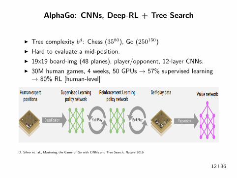
AlphaGo CNNs Deep-RL + Tree Search
I Tree complexity bd Chess (3580) Go (250150)
I Hard to evaluate a mid-position
I 19x19 board-img (48 planes) playeropponent 12-layer CNNs
I 30M human games 4 weeks 50 GPUs rarr 57 supervised learningrarr 80 RL [human-level]
D Silver et al Mastering the Game of Go with DNNs and Tree Search Nature 2016
12 36
AlphaGo CNNs Deep-RL + Tree Search
I Tree complexity bd Chess (3580) Go (250150)
I Hard to evaluate a mid-position
I 19x19 board-img (48 planes) playeropponent 12-layer CNNs
I 30M human games 4 weeks 50 GPUs rarr 57 supervised learningrarr 80 RL [human-level]
D Silver et al Mastering the Game of Go with DNNs and Tree Search Nature 2016
12 36
AlphaGo CNNs Deep-RL + Tree Search
I Tree complexity bd Chess (3580) Go (250150)
I Hard to evaluate a mid-position
I 19x19 board-img (48 planes) playeropponent 12-layer CNNs
I 30M human games 4 weeks 50 GPUs rarr 57 supervised learningrarr 80 RL [human-level]
D Silver et al Mastering the Game of Go with DNNs and Tree Search Nature 2016
12 36
Machine Learning in 1990s
I Convolutional Neural Networks (Fukushima 1980 Lecun et al 1989)
ndash 3 days to train on USPS (n = 7291 digit recognition) on SunSparcstation 1 (33MHz clock speed 64MB RAM)
I Personal history
ndash 1998 (Deep Blue Google Email) Train DNN on UCI Wine datasetndash 1999 Introduced to Kernel Methods - by DNN researchersndash 2003-4 NN paper at JMLR rejected accepted in IEEE Trans
Neural Nets with a kernel methods section
I Why Kernel Methods
ndash Local Minima free - stronger role of Convex Optimizationndash Theoretically appealingndash Handle non-vectorial data high-dimensional datandash Easier model selection via continuous optimizationndash Matched NN in many cases although didnt scale wrt n as well
I So what changed
ndash More data parallel algorithms hardware Better DNN training
13 36
Machine Learning in 1990s
I Convolutional Neural Networks (Fukushima 1980 Lecun et al 1989)
ndash 3 days to train on USPS (n = 7291 digit recognition) on SunSparcstation 1 (33MHz clock speed 64MB RAM)
I Personal history
ndash 1998 (Deep Blue Google Email) Train DNN on UCI Wine dataset
ndash 1999 Introduced to Kernel Methods - by DNN researchersndash 2003-4 NN paper at JMLR rejected accepted in IEEE Trans
Neural Nets with a kernel methods section
I Why Kernel Methods
ndash Local Minima free - stronger role of Convex Optimizationndash Theoretically appealingndash Handle non-vectorial data high-dimensional datandash Easier model selection via continuous optimizationndash Matched NN in many cases although didnt scale wrt n as well
I So what changed
ndash More data parallel algorithms hardware Better DNN training
13 36
Machine Learning in 1990s
I Convolutional Neural Networks (Fukushima 1980 Lecun et al 1989)
ndash 3 days to train on USPS (n = 7291 digit recognition) on SunSparcstation 1 (33MHz clock speed 64MB RAM)
I Personal history
ndash 1998 (Deep Blue Google Email) Train DNN on UCI Wine datasetndash 1999 Introduced to Kernel Methods - by DNN researchers
ndash 2003-4 NN paper at JMLR rejected accepted in IEEE TransNeural Nets with a kernel methods section
I Why Kernel Methods
ndash Local Minima free - stronger role of Convex Optimizationndash Theoretically appealingndash Handle non-vectorial data high-dimensional datandash Easier model selection via continuous optimizationndash Matched NN in many cases although didnt scale wrt n as well
I So what changed
ndash More data parallel algorithms hardware Better DNN training
13 36
Machine Learning in 1990s
I Convolutional Neural Networks (Fukushima 1980 Lecun et al 1989)
ndash 3 days to train on USPS (n = 7291 digit recognition) on SunSparcstation 1 (33MHz clock speed 64MB RAM)
I Personal history
ndash 1998 (Deep Blue Google Email) Train DNN on UCI Wine datasetndash 1999 Introduced to Kernel Methods - by DNN researchersndash 2003-4 NN paper at JMLR rejected accepted in IEEE Trans
Neural Nets with a kernel methods section
I Why Kernel Methods
ndash Local Minima free - stronger role of Convex Optimizationndash Theoretically appealingndash Handle non-vectorial data high-dimensional datandash Easier model selection via continuous optimizationndash Matched NN in many cases although didnt scale wrt n as well
I So what changed
ndash More data parallel algorithms hardware Better DNN training
13 36
Machine Learning in 1990s
I Convolutional Neural Networks (Fukushima 1980 Lecun et al 1989)
ndash 3 days to train on USPS (n = 7291 digit recognition) on SunSparcstation 1 (33MHz clock speed 64MB RAM)
I Personal history
ndash 1998 (Deep Blue Google Email) Train DNN on UCI Wine datasetndash 1999 Introduced to Kernel Methods - by DNN researchersndash 2003-4 NN paper at JMLR rejected accepted in IEEE Trans
Neural Nets with a kernel methods section
I Why Kernel Methods
ndash Local Minima free - stronger role of Convex Optimizationndash Theoretically appealingndash Handle non-vectorial data high-dimensional datandash Easier model selection via continuous optimizationndash Matched NN in many cases although didnt scale wrt n as well
I So what changed
ndash More data parallel algorithms hardware Better DNN training
13 36
Machine Learning in 1990s
I Convolutional Neural Networks (Fukushima 1980 Lecun et al 1989)
ndash 3 days to train on USPS (n = 7291 digit recognition) on SunSparcstation 1 (33MHz clock speed 64MB RAM)
I Personal history
ndash 1998 (Deep Blue Google Email) Train DNN on UCI Wine datasetndash 1999 Introduced to Kernel Methods - by DNN researchersndash 2003-4 NN paper at JMLR rejected accepted in IEEE Trans
Neural Nets with a kernel methods section
I Why Kernel Methods
ndash Local Minima free - stronger role of Convex Optimization
ndash Theoretically appealingndash Handle non-vectorial data high-dimensional datandash Easier model selection via continuous optimizationndash Matched NN in many cases although didnt scale wrt n as well
I So what changed
ndash More data parallel algorithms hardware Better DNN training
13 36
Machine Learning in 1990s
I Convolutional Neural Networks (Fukushima 1980 Lecun et al 1989)
ndash 3 days to train on USPS (n = 7291 digit recognition) on SunSparcstation 1 (33MHz clock speed 64MB RAM)
I Personal history
ndash 1998 (Deep Blue Google Email) Train DNN on UCI Wine datasetndash 1999 Introduced to Kernel Methods - by DNN researchersndash 2003-4 NN paper at JMLR rejected accepted in IEEE Trans
Neural Nets with a kernel methods section
I Why Kernel Methods
ndash Local Minima free - stronger role of Convex Optimizationndash Theoretically appealing
ndash Handle non-vectorial data high-dimensional datandash Easier model selection via continuous optimizationndash Matched NN in many cases although didnt scale wrt n as well
I So what changed
ndash More data parallel algorithms hardware Better DNN training
13 36
Machine Learning in 1990s
I Convolutional Neural Networks (Fukushima 1980 Lecun et al 1989)
ndash 3 days to train on USPS (n = 7291 digit recognition) on SunSparcstation 1 (33MHz clock speed 64MB RAM)
I Personal history
ndash 1998 (Deep Blue Google Email) Train DNN on UCI Wine datasetndash 1999 Introduced to Kernel Methods - by DNN researchersndash 2003-4 NN paper at JMLR rejected accepted in IEEE Trans
Neural Nets with a kernel methods section
I Why Kernel Methods
ndash Local Minima free - stronger role of Convex Optimizationndash Theoretically appealingndash Handle non-vectorial data high-dimensional datandash Easier model selection via continuous optimization
ndash Matched NN in many cases although didnt scale wrt n as well
I So what changed
ndash More data parallel algorithms hardware Better DNN training
13 36
Machine Learning in 1990s
I Convolutional Neural Networks (Fukushima 1980 Lecun et al 1989)
ndash 3 days to train on USPS (n = 7291 digit recognition) on SunSparcstation 1 (33MHz clock speed 64MB RAM)
I Personal history
ndash 1998 (Deep Blue Google Email) Train DNN on UCI Wine datasetndash 1999 Introduced to Kernel Methods - by DNN researchersndash 2003-4 NN paper at JMLR rejected accepted in IEEE Trans
Neural Nets with a kernel methods section
I Why Kernel Methods
ndash Local Minima free - stronger role of Convex Optimizationndash Theoretically appealingndash Handle non-vectorial data high-dimensional datandash Easier model selection via continuous optimizationndash Matched NN in many cases although didnt scale wrt n as well
I So what changed
ndash More data parallel algorithms hardware Better DNN training
13 36
Machine Learning in 1990s
I Convolutional Neural Networks (Fukushima 1980 Lecun et al 1989)
ndash 3 days to train on USPS (n = 7291 digit recognition) on SunSparcstation 1 (33MHz clock speed 64MB RAM)
I Personal history
ndash 1998 (Deep Blue Google Email) Train DNN on UCI Wine datasetndash 1999 Introduced to Kernel Methods - by DNN researchersndash 2003-4 NN paper at JMLR rejected accepted in IEEE Trans
Neural Nets with a kernel methods section
I Why Kernel Methods
ndash Local Minima free - stronger role of Convex Optimizationndash Theoretically appealingndash Handle non-vectorial data high-dimensional datandash Easier model selection via continuous optimizationndash Matched NN in many cases although didnt scale wrt n as well
I So what changed
ndash More data parallel algorithms hardware Better DNN training
13 36
Kernel Methods vs Neural Networks (Pre-Google)
14 36
Kernel Methods vs Neural Networks
Geoff Hinton facts meme maintained athttpyannlecuncomexfun
I All kernels that ever dared approaching Geoff Hinton woke upconvolved
I The only kernel Geoff Hinton has ever used is a kernel of truth
I If you defy Geoff Hinton he will maximize your entropy in no timeYour free energy will be gone even before you reach equilibrium
Are there synergies between these fields towards design of even better(faster and more accurate) algorithms
15 36
Kernel Methods vs Neural Networks
Geoff Hinton facts meme maintained athttpyannlecuncomexfun
I All kernels that ever dared approaching Geoff Hinton woke upconvolved
I The only kernel Geoff Hinton has ever used is a kernel of truth
I If you defy Geoff Hinton he will maximize your entropy in no timeYour free energy will be gone even before you reach equilibrium
Are there synergies between these fields towards design of even better(faster and more accurate) algorithms
15 36
Kernel Methods vs Neural Networks
Geoff Hinton facts meme maintained athttpyannlecuncomexfun
I All kernels that ever dared approaching Geoff Hinton woke upconvolved
I The only kernel Geoff Hinton has ever used is a kernel of truth
I If you defy Geoff Hinton he will maximize your entropy in no timeYour free energy will be gone even before you reach equilibrium
Are there synergies between these fields towards design of even better(faster and more accurate) algorithms
15 36
Linear Hypotheses
I f(x) = wTxw isin Rn Assume Y sub R setting
arg minwisinRd
lsumi=1
(yi minuswTxi)2 + λw22
w = (XTX + λId)minus1 (XTy
)X =
xTi
isin Rltimesn
I ntimes n linear system =rArr O(ln2 + n3) training time assuming nostructure (eg sparsity)
I O(n) prediction time
I High Approximation error
16 36
Polynomials The expensive way
I Homogeneous degree-d polynomial
f(x) = wTΨnd(x) w isin Rs s =
(d+ nminus 1
d
)
Ψnd(x) =
radic(dα
)xα
isin Rs
α = (α1 αn)sumi
αi = d
(d
α
)=
d
α1 αn
xα = xα11 xα2
2 xαnn
I Construct Z isin Rntimess with rows Ψnd(xi) and solve in O(s3) () time
w = (ZTZ + λId)minus1 (ZTy) (1)
I Note n = 100 d = 4 =rArr s gt 4M
17 36
Polynomials
I Consider the subspace of Rs spanned by the data
S = span (Ψ(x1) Ψ(xl)) = v isin Rs v =
lsumi=1
αiΨ(xi)
I So Rs = S + Sperp Hence for any vector w isin Rs
w = wS + wSperp
I The search of a minimizer can be reduced to S because
lsumi=1
V (wTΨ(xi)) + λw22 gelsumi=1
V (wTSΨ(xi)) + λwS22 + wperpS 22
gelsumi=1
V (wTSΨ(xi)) + λwS22 (2)
I Argument holds for any loss (convex or non-convex additive or not)but needs orthogonality (l2 regularizer) [Representer Theorem]
18 36
Polynomials
I Consider the subspace of Rs spanned by the data
S = span (Ψ(x1) Ψ(xl)) = v isin Rs v =
lsumi=1
αiΨ(xi)
I So Rs = S + Sperp Hence for any vector w isin Rs
w = wS + wSperp
I The search of a minimizer can be reduced to S because
lsumi=1
V (wTΨ(xi)) + λw22 gelsumi=1
V (wTSΨ(xi)) + λwS22 + wperpS 22
gelsumi=1
V (wTSΨ(xi)) + λwS22 (2)
I Argument holds for any loss (convex or non-convex additive or not)but needs orthogonality (l2 regularizer) [Representer Theorem]
18 36
Polynomials
I Consider the subspace of Rs spanned by the data
S = span (Ψ(x1) Ψ(xl)) = v isin Rs v =
lsumi=1
αiΨ(xi)
I So Rs = S + Sperp Hence for any vector w isin Rs
w = wS + wSperp
I The search of a minimizer can be reduced to S because
lsumi=1
V (wTΨ(xi)) + λw22 gelsumi=1
V (wTSΨ(xi)) + λwS22 + wperpS 22
gelsumi=1
V (wTSΨ(xi)) + λwS22 (2)
I Argument holds for any loss (convex or non-convex additive or not)but needs orthogonality (l2 regularizer) [Representer Theorem]
18 36
Polynomials
I Consider the subspace of Rs spanned by the data
S = span (Ψ(x1) Ψ(xl)) = v isin Rs v =
lsumi=1
αiΨ(xi)
I So Rs = S + Sperp Hence for any vector w isin Rs
w = wS + wSperp
I The search of a minimizer can be reduced to S because
lsumi=1
V (wTΨ(xi)) + λw22 gelsumi=1
V (wTSΨ(xi)) + λwS22 + wperpS 22
gelsumi=1
V (wTSΨ(xi)) + λwS22 (2)
I Argument holds for any loss (convex or non-convex additive or not)but needs orthogonality (l2 regularizer) [Representer Theorem]
18 36
Polynomials
I Hence w =sumli=1 βiΨ(xi) isin S for β isin Rl and so we can solve
arg minwisinRd
lsumi=1
(yi minuswTΨ(xi))2 + λw22
arg minβisinRl
lsumj=1
(yj minus
lsumi=1
βiΨ(xi)TΨ(xj)
)2
+ λ
lsumij=1
βiβjΨ(xi)TΨ(xj)
arg minβisinRl
lsumj=1
(yj minus (Gβ)j
)2+ λβTGβ
Gij = Ψ(xi)TΨ(xj)
β = (G + λId)minus1
y
I O(l3 + sl2) training time - O(s3) cost eliminatedI Inference time (O(s) or O(ls))
f(x) = wTΨ(x) =
lsumi=1
βiΨ(xi)TΨ(x)
19 36
Polynomials
I Hence w =sumli=1 βiΨ(xi) isin S for β isin Rl and so we can solve
arg minwisinRd
lsumi=1
(yi minuswTΨ(xi))2 + λw22
arg minβisinRl
lsumj=1
(yj minus
lsumi=1
βiΨ(xi)TΨ(xj)
)2
+ λ
lsumij=1
βiβjΨ(xi)TΨ(xj)
arg minβisinRl
lsumj=1
(yj minus (Gβ)j
)2+ λβTGβ
Gij = Ψ(xi)TΨ(xj)
β = (G + λId)minus1
y
I O(l3 + sl2) training time - O(s3) cost eliminatedI Inference time (O(s) or O(ls))
f(x) = wTΨ(x) =
lsumi=1
βiΨ(xi)TΨ(x)
19 36
Polynomials
I Hence w =sumli=1 βiΨ(xi) isin S for β isin Rl and so we can solve
arg minwisinRd
lsumi=1
(yi minuswTΨ(xi))2 + λw22
arg minβisinRl
lsumj=1
(yj minus
lsumi=1
βiΨ(xi)TΨ(xj)
)2
+ λ
lsumij=1
βiβjΨ(xi)TΨ(xj)
arg minβisinRl
lsumj=1
(yj minus (Gβ)j
)2+ λβTGβ
Gij = Ψ(xi)TΨ(xj)
β = (G + λId)minus1
y
I O(l3 + sl2) training time - O(s3) cost eliminatedI Inference time (O(s) or O(ls))
f(x) = wTΨ(x) =
lsumi=1
βiΨ(xi)TΨ(x)
19 36
Polynomials
I Multinomial Theorem
(z1 + z2 + + zn)d =sum
α|α|=d
(d
α
)zα
I Implicit computation of inner products
Ψ(x)TΨ(xprime) =
ssumi=1
(d
α
)xαxprime
α=
ssumi=1
(d
α
)xα11 xαnn x
primeα11 x
primeαnn
=
ssumi=1
(d
α
)(x1x
prime1)α1(x2x
prime2)α2 (xnx
primen)αn
= (x1xprime1 + xnx
primen)d
= (xTxprime)d
I O(l3 + l2n) training and O(ln) predicting speedI Complexity coming from s has been completely eliminated ()
[Kernel Trick]
20 36
Polynomials
I Multinomial Theorem
(z1 + z2 + + zn)d =sum
α|α|=d
(d
α
)zα
I Implicit computation of inner products
Ψ(x)TΨ(xprime) =
ssumi=1
(d
α
)xαxprime
α=
ssumi=1
(d
α
)xα11 xαnn x
primeα11 x
primeαnn
=
ssumi=1
(d
α
)(x1x
prime1)α1(x2x
prime2)α2 (xnx
primen)αn
= (x1xprime1 + xnx
primen)d
= (xTxprime)d
I O(l3 + l2n) training and O(ln) predicting speedI Complexity coming from s has been completely eliminated ()
[Kernel Trick]
20 36
Polynomials
I Multinomial Theorem
(z1 + z2 + + zn)d =sum
α|α|=d
(d
α
)zα
I Implicit computation of inner products
Ψ(x)TΨ(xprime) =
ssumi=1
(d
α
)xαxprime
α=
ssumi=1
(d
α
)xα11 xαnn x
primeα11 x
primeαnn
=
ssumi=1
(d
α
)(x1x
prime1)α1(x2x
prime2)α2 (xnx
primen)αn
= (x1xprime1 + xnx
primen)d
= (xTxprime)d
I O(l3 + l2n) training and O(ln) predicting speedI Complexity coming from s has been completely eliminated ()
[Kernel Trick]
20 36
Polynomials
I Multinomial Theorem
(z1 + z2 + + zn)d =sum
α|α|=d
(d
α
)zα
I Implicit computation of inner products
Ψ(x)TΨ(xprime) =
ssumi=1
(d
α
)xαxprime
α=
ssumi=1
(d
α
)xα11 xαnn x
primeα11 x
primeαnn
=
ssumi=1
(d
α
)(x1x
prime1)α1(x2x
prime2)α2 (xnx
primen)αn
= (x1xprime1 + xnx
primen)d
= (xTxprime)d
I O(l3 + l2n) training and O(ln) predicting speedI Complexity coming from s has been completely eliminated ()
[Kernel Trick]
20 36
Polynomials
I Multinomial Theorem
(z1 + z2 + + zn)d =sum
α|α|=d
(d
α
)zα
I Implicit computation of inner products
Ψ(x)TΨ(xprime) =
ssumi=1
(d
α
)xαxprime
α=
ssumi=1
(d
α
)xα11 xαnn x
primeα11 x
primeαnn
=
ssumi=1
(d
α
)(x1x
prime1)α1(x2x
prime2)α2 (xnx
primen)αn
= (x1xprime1 + xnx
primen)d
= (xTxprime)d
I O(l3 + l2n) training and O(ln) predicting speedI Complexity coming from s has been completely eliminated ()
[Kernel Trick]
20 36
Polynomials Algorithm
I Algorithm
ndash Start with k X times X 7rarr R k(xxprime) = (xTxprime + 1)d
ndash Construct Gram matrix Gij = k(xixj) on the training samplesndash Solve β = (G + λId)minus1 yndash Return f(x) =
sumli=1 βik(xix)
I f is the optimal degree-d polynomial solving the learning problemin complexity independent of d
I What other forms of k correspond to linear learning inhigh-dimensional nonlinear embeddings of the data
21 36
Polynomials Algorithm
I Algorithm
ndash Start with k X times X 7rarr R k(xxprime) = (xTxprime + 1)d
ndash Construct Gram matrix Gij = k(xixj) on the training samplesndash Solve β = (G + λId)minus1 yndash Return f(x) =
sumli=1 βik(xix)
I f is the optimal degree-d polynomial solving the learning problemin complexity independent of d
I What other forms of k correspond to linear learning inhigh-dimensional nonlinear embeddings of the data
21 36
Symmetric positive semi-definite functions
I Definition A function k X times X 7rarr R is psd if for any finitecollection of points x1 xl the l times l Gram matrix
Gij = k(xixj)
is positive semi-definite ie for any vector β isin Rl
βTGβ =sumij
βiβjk(xixj) ge 0
I Theorem[Mercer] If k is symmetric psd X is compact subset ofRn then it admits an eigenfunction decomposition
k(xxprime) =
Nsumi=1
λiφj(x)φj(xprime) = 〈Ψ(x)Ψ(xprime)〉l2
Ψ(x) = [ radicλjφ(x) ]T (3)
I Feature map associated with a kernel is not uniqueI Functional generalization of positive semi-definite matrices
22 36
Symmetric positive semi-definite functions
I Definition A function k X times X 7rarr R is psd if for any finitecollection of points x1 xl the l times l Gram matrix
Gij = k(xixj)
is positive semi-definite ie for any vector β isin Rl
βTGβ =sumij
βiβjk(xixj) ge 0
I Theorem[Mercer] If k is symmetric psd X is compact subset ofRn then it admits an eigenfunction decomposition
k(xxprime) =
Nsumi=1
λiφj(x)φj(xprime) = 〈Ψ(x)Ψ(xprime)〉l2
Ψ(x) = [ radicλjφ(x) ]T (3)
I Feature map associated with a kernel is not uniqueI Functional generalization of positive semi-definite matrices
22 36
Kernels
I Lineark(xxprime) = xTxprime
I Polynomialk(xxprime) = (xTxprime + 1)d
I Gaussian s =infin Universal
k(xxprime) = eminusxminusxprime2
2σ2
I Conic combinations
k(xxprime) = α1k1(xxprime) + α2k2(xxprime)
I Elementwise products
k(xxprime) = k1(xxprime)k2(xxprime)
I Kernels on discrete sets strings graphs sequences shapes
23 36
Kernels
I Lineark(xxprime) = xTxprime
I Polynomialk(xxprime) = (xTxprime + 1)d
I Gaussian s =infin Universal
k(xxprime) = eminusxminusxprime2
2σ2
I Conic combinations
k(xxprime) = α1k1(xxprime) + α2k2(xxprime)
I Elementwise products
k(xxprime) = k1(xxprime)k2(xxprime)
I Kernels on discrete sets strings graphs sequences shapes
23 36
Kernels
I Lineark(xxprime) = xTxprime
I Polynomialk(xxprime) = (xTxprime + 1)d
I Gaussian s =infin Universal
k(xxprime) = eminusxminusxprime2
2σ2
I Conic combinations
k(xxprime) = α1k1(xxprime) + α2k2(xxprime)
I Elementwise products
k(xxprime) = k1(xxprime)k2(xxprime)
I Kernels on discrete sets strings graphs sequences shapes
23 36
Gaussian Kernel is Positive Definite
I Exponential
eβxTxprime = 1 + βxTxprime +
β2
2(xTy)2 +
β3
3(xTy)3 +
I For any function f Rn 7rarr R psd function k the following kernelis psd
kprime(xxprime) = f(x) (k(xxprime)) f(xprime)
Proofsumij
βiβjkprime(xixj) =
sumij
βiβjf(xi)k(xixj)f(xj) =sumij
βprimeiβprimejk(xixj) ge 0
I Gaussian Kernel
k(xxprime) = eminusxminusxprime22
2σ2
= eminusx222σ2
(e
2xT xprime2σ2
)eminusxprime222σ2 (4)
24 36
Gaussian Kernel is Positive Definite
I Exponential
eβxTxprime = 1 + βxTxprime +
β2
2(xTy)2 +
β3
3(xTy)3 +
I For any function f Rn 7rarr R psd function k the following kernelis psd
kprime(xxprime) = f(x) (k(xxprime)) f(xprime)
Proofsumij
βiβjkprime(xixj) =
sumij
βiβjf(xi)k(xixj)f(xj) =sumij
βprimeiβprimejk(xixj) ge 0
I Gaussian Kernel
k(xxprime) = eminusxminusxprime22
2σ2
= eminusx222σ2
(e
2xT xprime2σ2
)eminusxprime222σ2 (4)
24 36
Gaussian Kernel is Positive Definite
I Exponential
eβxTxprime = 1 + βxTxprime +
β2
2(xTy)2 +
β3
3(xTy)3 +
I For any function f Rn 7rarr R psd function k the following kernelis psd
kprime(xxprime) = f(x) (k(xxprime)) f(xprime)
Proofsumij
βiβjkprime(xixj) =
sumij
βiβjf(xi)k(xixj)f(xj) =sumij
βprimeiβprimejk(xixj) ge 0
I Gaussian Kernel
k(xxprime) = eminusxminusxprime22
2σ2
= eminusx222σ2
(e
2xT xprime2σ2
)eminusxprime222σ2 (4)
24 36
The Mathematical Naturalness of Kernel Methods
I Data X isin Rd Models isin H X 7rarr R
I Geometry in H inner product 〈middot middot〉H norm middot H (Hilbert Spaces)I Theorem All nice Hilbert spaces are generated by a symmetric
positive definite function (the kernel) k(xxprime) on X times XI if f g isin H close ie f minus gH small then f(x) g(x) close forallx isin X I Reproducing Kernel Hilbert Spaces (RKHSs) Hilbert space H
that admit a reproducing kernel ie a function k(xxprime) satisfying
(i) forallx isin X k(middotx) isin H(ii) 〈f k(middotx)〉H = f(x)
I Reproducing kernels are symmetric psdsumij
βiβjk(xixj) = 〈sumi
βik(middotxi)sumi
βik(middotxi)〉H
= sumi
βik(middotxi)2H ge 0 (5)
I (Moore-Aronsjan 1950) Symmetric psd functions arereproducing kernels for some (unique) RKHS Hk
25 36
The Mathematical Naturalness of Kernel Methods
I Data X isin Rd Models isin H X 7rarr RI Geometry in H inner product 〈middot middot〉H norm middot H (Hilbert Spaces)
I Theorem All nice Hilbert spaces are generated by a symmetricpositive definite function (the kernel) k(xxprime) on X times X
I if f g isin H close ie f minus gH small then f(x) g(x) close forallx isin X I Reproducing Kernel Hilbert Spaces (RKHSs) Hilbert space H
that admit a reproducing kernel ie a function k(xxprime) satisfying
(i) forallx isin X k(middotx) isin H(ii) 〈f k(middotx)〉H = f(x)
I Reproducing kernels are symmetric psdsumij
βiβjk(xixj) = 〈sumi
βik(middotxi)sumi
βik(middotxi)〉H
= sumi
βik(middotxi)2H ge 0 (5)
I (Moore-Aronsjan 1950) Symmetric psd functions arereproducing kernels for some (unique) RKHS Hk
25 36
The Mathematical Naturalness of Kernel Methods
I Data X isin Rd Models isin H X 7rarr RI Geometry in H inner product 〈middot middot〉H norm middot H (Hilbert Spaces)I Theorem All nice Hilbert spaces are generated by a symmetric
positive definite function (the kernel) k(xxprime) on X times XI if f g isin H close ie f minus gH small then f(x) g(x) close forallx isin X
I Reproducing Kernel Hilbert Spaces (RKHSs) Hilbert space Hthat admit a reproducing kernel ie a function k(xxprime) satisfying
(i) forallx isin X k(middotx) isin H(ii) 〈f k(middotx)〉H = f(x)
I Reproducing kernels are symmetric psdsumij
βiβjk(xixj) = 〈sumi
βik(middotxi)sumi
βik(middotxi)〉H
= sumi
βik(middotxi)2H ge 0 (5)
I (Moore-Aronsjan 1950) Symmetric psd functions arereproducing kernels for some (unique) RKHS Hk
25 36
The Mathematical Naturalness of Kernel Methods
I Data X isin Rd Models isin H X 7rarr RI Geometry in H inner product 〈middot middot〉H norm middot H (Hilbert Spaces)I Theorem All nice Hilbert spaces are generated by a symmetric
positive definite function (the kernel) k(xxprime) on X times XI if f g isin H close ie f minus gH small then f(x) g(x) close forallx isin X I Reproducing Kernel Hilbert Spaces (RKHSs) Hilbert space H
that admit a reproducing kernel ie a function k(xxprime) satisfying
(i) forallx isin X k(middotx) isin H(ii) 〈f k(middotx)〉H = f(x)
I Reproducing kernels are symmetric psdsumij
βiβjk(xixj) = 〈sumi
βik(middotxi)sumi
βik(middotxi)〉H
= sumi
βik(middotxi)2H ge 0 (5)
I (Moore-Aronsjan 1950) Symmetric psd functions arereproducing kernels for some (unique) RKHS Hk
25 36
The Mathematical Naturalness of Kernel Methods
I Data X isin Rd Models isin H X 7rarr RI Geometry in H inner product 〈middot middot〉H norm middot H (Hilbert Spaces)I Theorem All nice Hilbert spaces are generated by a symmetric
positive definite function (the kernel) k(xxprime) on X times XI if f g isin H close ie f minus gH small then f(x) g(x) close forallx isin X I Reproducing Kernel Hilbert Spaces (RKHSs) Hilbert space H
that admit a reproducing kernel ie a function k(xxprime) satisfying
(i) forallx isin X k(middotx) isin H(ii) 〈f k(middotx)〉H = f(x)
I Reproducing kernels are symmetric psdsumij
βiβjk(xixj) = 〈sumi
βik(middotxi)sumi
βik(middotxi)〉H
= sumi
βik(middotxi)2H ge 0 (5)
I (Moore-Aronsjan 1950) Symmetric psd functions arereproducing kernels for some (unique) RKHS Hk 25 36
Kernel Methods Summary
I Symm pos def function k(x z) on input domain X sub Rd
I k hArr rich Reproducing Kernel Hilbert Space (RKHS) Hk ofreal-valued functions with inner product 〈middot middot〉k and norm middot k
I Regularized Risk Minimization hArr Linear models in an implicithigh-dimensional (often infinite-dimensional) feature space
f = arg minfisinHk
1
n
nsumi=1
V (yi f(xi)) + λf2Hk xi isin Rd
I Representer Theorem f(x) =sumni=1 αik(xxi)
26 36
Shallow and Deep Function Spaces
I What does it mean to understand a function space
ndash Linear f(x) = wTxw isin Rd
ndash Polynomial f(x) = wT Ψ(x)w isin Rs
ndash RKHS balls f isin Hk fk lt γ [like vM le 1]
I Shallow nets f(x) = wTσ(Wx) (w isin RdW isin Rs)ndash For srarrinfin W sim p σ(u) = eminusiu approximates Gaussian kernel
methodsndash Theorem [Bochner 1937] One-to-one correspondence between k
and a density p such that
k(x z) = ψ(xminus z) =
intRdeminusi(xminusz)Twp(w)dw asymp 1
s
ssumj=1
eminusi(xminusz)Twj
Gaussian kernel k(x z) = eminusxminusz22
2σ2 lArrrArr p = N (0 σminus2Id)ndash Similar integral approx relates ReLU to the arc-cosine kernelndash Optimization versus Randomization
27 36
Shallow and Deep Function Spaces
I What does it mean to understand a function space
ndash Linear f(x) = wTxw isin Rd
ndash Polynomial f(x) = wT Ψ(x)w isin Rs
ndash RKHS balls f isin Hk fk lt γ [like vM le 1]
I Shallow nets f(x) = wTσ(Wx) (w isin RdW isin Rs)ndash For srarrinfin W sim p σ(u) = eminusiu approximates Gaussian kernel
methodsndash Theorem [Bochner 1937] One-to-one correspondence between k
and a density p such that
k(x z) = ψ(xminus z) =
intRdeminusi(xminusz)Twp(w)dw asymp 1
s
ssumj=1
eminusi(xminusz)Twj
Gaussian kernel k(x z) = eminusxminusz22
2σ2 lArrrArr p = N (0 σminus2Id)ndash Similar integral approx relates ReLU to the arc-cosine kernelndash Optimization versus Randomization
27 36
Shallow and Deep Function Spaces
I What does it mean to understand a function space
ndash Linear f(x) = wTxw isin Rd
ndash Polynomial f(x) = wT Ψ(x)w isin Rs
ndash RKHS balls f isin Hk fk lt γ [like vM le 1]
I Shallow nets f(x) = wTσ(Wx) (w isin RdW isin Rs)ndash For srarrinfin W sim p σ(u) = eminusiu approximates Gaussian kernel
methodsndash Theorem [Bochner 1937] One-to-one correspondence between k
and a density p such that
k(x z) = ψ(xminus z) =
intRdeminusi(xminusz)Twp(w)dw asymp 1
s
ssumj=1
eminusi(xminusz)Twj
Gaussian kernel k(x z) = eminusxminusz22
2σ2 lArrrArr p = N (0 σminus2Id)ndash Similar integral approx relates ReLU to the arc-cosine kernelndash Optimization versus Randomization
27 36
Shallow and Deep Function Spaces
I What does it mean to understand a function space
ndash Linear f(x) = wTxw isin Rd
ndash Polynomial f(x) = wT Ψ(x)w isin Rs
ndash RKHS balls f isin Hk fk lt γ [like vM le 1]
I Shallow nets f(x) = wTσ(Wx) (w isin RdW isin Rs)
ndash For srarrinfin W sim p σ(u) = eminusiu approximates Gaussian kernelmethods
ndash Theorem [Bochner 1937] One-to-one correspondence between kand a density p such that
k(x z) = ψ(xminus z) =
intRdeminusi(xminusz)Twp(w)dw asymp 1
s
ssumj=1
eminusi(xminusz)Twj
Gaussian kernel k(x z) = eminusxminusz22
2σ2 lArrrArr p = N (0 σminus2Id)ndash Similar integral approx relates ReLU to the arc-cosine kernelndash Optimization versus Randomization
27 36
Shallow and Deep Function Spaces
I What does it mean to understand a function space
ndash Linear f(x) = wTxw isin Rd
ndash Polynomial f(x) = wT Ψ(x)w isin Rs
ndash RKHS balls f isin Hk fk lt γ [like vM le 1]
I Shallow nets f(x) = wTσ(Wx) (w isin RdW isin Rs)ndash For srarrinfin W sim p σ(u) = eminusiu approximates Gaussian kernel
methodsndash Theorem [Bochner 1937] One-to-one correspondence between k
and a density p such that
k(x z) = ψ(xminus z) =
intRdeminusi(xminusz)Twp(w)dw asymp 1
s
ssumj=1
eminusi(xminusz)Twj
Gaussian kernel k(x z) = eminusxminusz22
2σ2 lArrrArr p = N (0 σminus2Id)ndash Similar integral approx relates ReLU to the arc-cosine kernelndash Optimization versus Randomization
27 36
Expressivity of Deep Nets Linear Regions
I The ReLU map f(x) = max(Wx 0)W isin Rwtimesn is piecewise linear
I A piece is a connected region (a convex polytope) of Rd with sharedsparsity pattern in activations
I (Zaslavsky 1975) Number of linear regions formed by an arrangement of
s hyperplanes in d-dimensions in general position issumd
i=0
(si
)I Composition of ReLU maps is also piecewise linear
I (Raghu et al 2017 Pascano et al 2014 Montufar 2014) Number oflinear regions grows as O(wnd) for a composition of d ReLU maps(nrarr brarr brarr b rarr b) each of width w
I (Safran and Shamir 2017)
ndash 1[x le 1] x isin Rd ε-accurate 3-layer network with O(dε) neurons but cannot be approximated with
accuracy higher than O(1d4) using 2-layer networks unless width is exponential in d
28 36
Expressivity of Deep Nets Linear Regions
I The ReLU map f(x) = max(Wx 0)W isin Rwtimesn is piecewise linear
I A piece is a connected region (a convex polytope) of Rd with sharedsparsity pattern in activations
I (Zaslavsky 1975) Number of linear regions formed by an arrangement of
s hyperplanes in d-dimensions in general position issumd
i=0
(si
)I Composition of ReLU maps is also piecewise linear
I (Raghu et al 2017 Pascano et al 2014 Montufar 2014) Number oflinear regions grows as O(wnd) for a composition of d ReLU maps(nrarr brarr brarr b rarr b) each of width w
I (Safran and Shamir 2017)
ndash 1[x le 1] x isin Rd ε-accurate 3-layer network with O(dε) neurons but cannot be approximated with
accuracy higher than O(1d4) using 2-layer networks unless width is exponential in d
28 36
Expressivity of Deep Nets Linear Regions
I The ReLU map f(x) = max(Wx 0)W isin Rwtimesn is piecewise linear
I A piece is a connected region (a convex polytope) of Rd with sharedsparsity pattern in activations
I (Zaslavsky 1975) Number of linear regions formed by an arrangement of
s hyperplanes in d-dimensions in general position issumd
i=0
(si
)
I Composition of ReLU maps is also piecewise linear
I (Raghu et al 2017 Pascano et al 2014 Montufar 2014) Number oflinear regions grows as O(wnd) for a composition of d ReLU maps(nrarr brarr brarr b rarr b) each of width w
I (Safran and Shamir 2017)
ndash 1[x le 1] x isin Rd ε-accurate 3-layer network with O(dε) neurons but cannot be approximated with
accuracy higher than O(1d4) using 2-layer networks unless width is exponential in d
28 36
Expressivity of Deep Nets Linear Regions
I The ReLU map f(x) = max(Wx 0)W isin Rwtimesn is piecewise linear
I A piece is a connected region (a convex polytope) of Rd with sharedsparsity pattern in activations
I (Zaslavsky 1975) Number of linear regions formed by an arrangement of
s hyperplanes in d-dimensions in general position issumd
i=0
(si
)I Composition of ReLU maps is also piecewise linear
I (Raghu et al 2017 Pascano et al 2014 Montufar 2014) Number oflinear regions grows as O(wnd) for a composition of d ReLU maps(nrarr brarr brarr b rarr b) each of width w
I (Safran and Shamir 2017)
ndash 1[x le 1] x isin Rd ε-accurate 3-layer network with O(dε) neurons but cannot be approximated with
accuracy higher than O(1d4) using 2-layer networks unless width is exponential in d28 36
Expressivity of Deep Nets Trajectory Length
I (Raghu et al 2017) Trajectory Length (ldquogeneralized operator normrdquo)How much is a curve in the input space stretched by a layer in thenetwork
29 36
Expressivity of Deep Nets Trajectory Length
I (Raghu et al 2017) Trajectory Length (ldquogeneralized operator normrdquo)How much is a curve in the input space stretched by a layer in thenetwork
29 36
Expressivity and Generalization
I Expressiveness equiv capacity to fit random noise =rArr susceptibility tooverfitting (VC dimension Rademacher Complexity)
I Zhang et al 2017 Famous CNNs easily fit random labels
ndash Over-parameterized (n=12M psim 60M) but structuredndash Domain-knowledge baked in does not constraint expressiveness
I CNNs tend to generalize even without regularization (explicit and implicit)
I For linear regression SGD returns minimum norm solution
30 36
Expressivity and Generalization
I Expressiveness equiv capacity to fit random noise =rArr susceptibility tooverfitting (VC dimension Rademacher Complexity)
I Zhang et al 2017 Famous CNNs easily fit random labels
ndash Over-parameterized (n=12M psim 60M) but structuredndash Domain-knowledge baked in does not constraint expressiveness
I CNNs tend to generalize even without regularization (explicit and implicit)
I For linear regression SGD returns minimum norm solution
30 36
Expressivity and Generalization
I Expressiveness equiv capacity to fit random noise =rArr susceptibility tooverfitting (VC dimension Rademacher Complexity)
I Zhang et al 2017 Famous CNNs easily fit random labels
ndash Over-parameterized (n=12M psim 60M) but structuredndash Domain-knowledge baked in does not constraint expressiveness
I CNNs tend to generalize even without regularization (explicit and implicit)
I For linear regression SGD returns minimum norm solution
30 36
Optimization Landscape Symmetry and Saddle Points
I Folklore lots of equivalent good local minI Classification of critical points based on Hessian spectrumI Permutation and Scaling symmetries
I Thm [Lee et al 2016 Anadkumar Ge] For the short-step gradientmethod the basin of attraction of strict saddle points (atleast onenegative eigenvalue) has measure zero
31 36
Optimization Landscape Symmetry and Saddle Points
I Folklore lots of equivalent good local minI Classification of critical points based on Hessian spectrumI Permutation and Scaling symmetries
I Thm [Lee et al 2016 Anadkumar Ge] For the short-step gradientmethod the basin of attraction of strict saddle points (atleast onenegative eigenvalue) has measure zero
31 36
Optimization Landscape Symmetry and Saddle Points
I Folklore lots of equivalent good local minI Classification of critical points based on Hessian spectrumI Permutation and Scaling symmetries
I Thm [Lee et al 2016 Anadkumar Ge] For the short-step gradientmethod the basin of attraction of strict saddle points (atleast onenegative eigenvalue) has measure zero
31 36
Optimization Landscape Sharp Minima and Stability
Keskar et al 2017 On large-batch training for DL Generalization Gap and Sharp Minima
32 36
Deep Learning Computational Graphs TensorFlow
tensorfloworg
I Tensors-in Tensors-out
I Evergrowing list of Tensor-Ops (PythonC++)
f(xw)
[partf
partx
]T v
[partf
partw
]T v
I Automatic Differentiation Reverse mode
partxL
partxi=sumirarrj
partxL
partxj
partxj
partxi
33 36
Computational Graphs and TensorFlow
tensorfloworg
I SGD with minibatches
wk+1 = wk minus ηlsumi=1
partli
partw
∣∣∣wt
I Model Parallelism Assign independent paths tothreads GPUs
I Data Parallelism create Graph replicas on differentmachines
I Mobile TensorFlow
34 36
Computational Graphs and TensorFlow
tensorfloworg
35 36
Computational Graphs and TensorFlow
tensorfloworg
35 36
Computational Graphs and TensorFlow
tensorfloworg
35 36
Challenges and Opportunities
I Lots of fascinating unsolved problems
I Can you win Imagenet with Convex optimization
I Tools from polynomial optimization (global optimization deep-RL)
I Supervised to Semi-supervised to Unsupervised Learning
I Compact efficient real-time models (eliminateover-parametrization) for new form factors
I Exciting emerging world of Robotics Wearable ComputersIntelligent home devices Personal digital assistants
Google Internship Program
36 36
- anm0
- fdrm0
- fdrm5
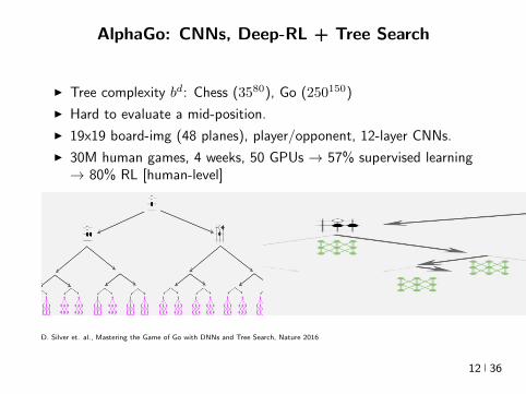
AlphaGo CNNs Deep-RL + Tree Search
I Tree complexity bd Chess (3580) Go (250150)
I Hard to evaluate a mid-position
I 19x19 board-img (48 planes) playeropponent 12-layer CNNs
I 30M human games 4 weeks 50 GPUs rarr 57 supervised learningrarr 80 RL [human-level]
D Silver et al Mastering the Game of Go with DNNs and Tree Search Nature 2016
12 36
AlphaGo CNNs Deep-RL + Tree Search
I Tree complexity bd Chess (3580) Go (250150)
I Hard to evaluate a mid-position
I 19x19 board-img (48 planes) playeropponent 12-layer CNNs
I 30M human games 4 weeks 50 GPUs rarr 57 supervised learningrarr 80 RL [human-level]
D Silver et al Mastering the Game of Go with DNNs and Tree Search Nature 2016
12 36
Machine Learning in 1990s
I Convolutional Neural Networks (Fukushima 1980 Lecun et al 1989)
ndash 3 days to train on USPS (n = 7291 digit recognition) on SunSparcstation 1 (33MHz clock speed 64MB RAM)
I Personal history
ndash 1998 (Deep Blue Google Email) Train DNN on UCI Wine datasetndash 1999 Introduced to Kernel Methods - by DNN researchersndash 2003-4 NN paper at JMLR rejected accepted in IEEE Trans
Neural Nets with a kernel methods section
I Why Kernel Methods
ndash Local Minima free - stronger role of Convex Optimizationndash Theoretically appealingndash Handle non-vectorial data high-dimensional datandash Easier model selection via continuous optimizationndash Matched NN in many cases although didnt scale wrt n as well
I So what changed
ndash More data parallel algorithms hardware Better DNN training
13 36
Machine Learning in 1990s
I Convolutional Neural Networks (Fukushima 1980 Lecun et al 1989)
ndash 3 days to train on USPS (n = 7291 digit recognition) on SunSparcstation 1 (33MHz clock speed 64MB RAM)
I Personal history
ndash 1998 (Deep Blue Google Email) Train DNN on UCI Wine dataset
ndash 1999 Introduced to Kernel Methods - by DNN researchersndash 2003-4 NN paper at JMLR rejected accepted in IEEE Trans
Neural Nets with a kernel methods section
I Why Kernel Methods
ndash Local Minima free - stronger role of Convex Optimizationndash Theoretically appealingndash Handle non-vectorial data high-dimensional datandash Easier model selection via continuous optimizationndash Matched NN in many cases although didnt scale wrt n as well
I So what changed
ndash More data parallel algorithms hardware Better DNN training
13 36
Machine Learning in 1990s
I Convolutional Neural Networks (Fukushima 1980 Lecun et al 1989)
ndash 3 days to train on USPS (n = 7291 digit recognition) on SunSparcstation 1 (33MHz clock speed 64MB RAM)
I Personal history
ndash 1998 (Deep Blue Google Email) Train DNN on UCI Wine datasetndash 1999 Introduced to Kernel Methods - by DNN researchers
ndash 2003-4 NN paper at JMLR rejected accepted in IEEE TransNeural Nets with a kernel methods section
I Why Kernel Methods
ndash Local Minima free - stronger role of Convex Optimizationndash Theoretically appealingndash Handle non-vectorial data high-dimensional datandash Easier model selection via continuous optimizationndash Matched NN in many cases although didnt scale wrt n as well
I So what changed
ndash More data parallel algorithms hardware Better DNN training
13 36
Machine Learning in 1990s
I Convolutional Neural Networks (Fukushima 1980 Lecun et al 1989)
ndash 3 days to train on USPS (n = 7291 digit recognition) on SunSparcstation 1 (33MHz clock speed 64MB RAM)
I Personal history
ndash 1998 (Deep Blue Google Email) Train DNN on UCI Wine datasetndash 1999 Introduced to Kernel Methods - by DNN researchersndash 2003-4 NN paper at JMLR rejected accepted in IEEE Trans
Neural Nets with a kernel methods section
I Why Kernel Methods
ndash Local Minima free - stronger role of Convex Optimizationndash Theoretically appealingndash Handle non-vectorial data high-dimensional datandash Easier model selection via continuous optimizationndash Matched NN in many cases although didnt scale wrt n as well
I So what changed
ndash More data parallel algorithms hardware Better DNN training
13 36
Machine Learning in 1990s
I Convolutional Neural Networks (Fukushima 1980 Lecun et al 1989)
ndash 3 days to train on USPS (n = 7291 digit recognition) on SunSparcstation 1 (33MHz clock speed 64MB RAM)
I Personal history
ndash 1998 (Deep Blue Google Email) Train DNN on UCI Wine datasetndash 1999 Introduced to Kernel Methods - by DNN researchersndash 2003-4 NN paper at JMLR rejected accepted in IEEE Trans
Neural Nets with a kernel methods section
I Why Kernel Methods
ndash Local Minima free - stronger role of Convex Optimizationndash Theoretically appealingndash Handle non-vectorial data high-dimensional datandash Easier model selection via continuous optimizationndash Matched NN in many cases although didnt scale wrt n as well
I So what changed
ndash More data parallel algorithms hardware Better DNN training
13 36
Machine Learning in 1990s
I Convolutional Neural Networks (Fukushima 1980 Lecun et al 1989)
ndash 3 days to train on USPS (n = 7291 digit recognition) on SunSparcstation 1 (33MHz clock speed 64MB RAM)
I Personal history
ndash 1998 (Deep Blue Google Email) Train DNN on UCI Wine datasetndash 1999 Introduced to Kernel Methods - by DNN researchersndash 2003-4 NN paper at JMLR rejected accepted in IEEE Trans
Neural Nets with a kernel methods section
I Why Kernel Methods
ndash Local Minima free - stronger role of Convex Optimization
ndash Theoretically appealingndash Handle non-vectorial data high-dimensional datandash Easier model selection via continuous optimizationndash Matched NN in many cases although didnt scale wrt n as well
I So what changed
ndash More data parallel algorithms hardware Better DNN training
13 36
Machine Learning in 1990s
I Convolutional Neural Networks (Fukushima 1980 Lecun et al 1989)
ndash 3 days to train on USPS (n = 7291 digit recognition) on SunSparcstation 1 (33MHz clock speed 64MB RAM)
I Personal history
ndash 1998 (Deep Blue Google Email) Train DNN on UCI Wine datasetndash 1999 Introduced to Kernel Methods - by DNN researchersndash 2003-4 NN paper at JMLR rejected accepted in IEEE Trans
Neural Nets with a kernel methods section
I Why Kernel Methods
ndash Local Minima free - stronger role of Convex Optimizationndash Theoretically appealing
ndash Handle non-vectorial data high-dimensional datandash Easier model selection via continuous optimizationndash Matched NN in many cases although didnt scale wrt n as well
I So what changed
ndash More data parallel algorithms hardware Better DNN training
13 36
Machine Learning in 1990s
I Convolutional Neural Networks (Fukushima 1980 Lecun et al 1989)
ndash 3 days to train on USPS (n = 7291 digit recognition) on SunSparcstation 1 (33MHz clock speed 64MB RAM)
I Personal history
ndash 1998 (Deep Blue Google Email) Train DNN on UCI Wine datasetndash 1999 Introduced to Kernel Methods - by DNN researchersndash 2003-4 NN paper at JMLR rejected accepted in IEEE Trans
Neural Nets with a kernel methods section
I Why Kernel Methods
ndash Local Minima free - stronger role of Convex Optimizationndash Theoretically appealingndash Handle non-vectorial data high-dimensional datandash Easier model selection via continuous optimization
ndash Matched NN in many cases although didnt scale wrt n as well
I So what changed
ndash More data parallel algorithms hardware Better DNN training
13 36
Machine Learning in 1990s
I Convolutional Neural Networks (Fukushima 1980 Lecun et al 1989)
ndash 3 days to train on USPS (n = 7291 digit recognition) on SunSparcstation 1 (33MHz clock speed 64MB RAM)
I Personal history
ndash 1998 (Deep Blue Google Email) Train DNN on UCI Wine datasetndash 1999 Introduced to Kernel Methods - by DNN researchersndash 2003-4 NN paper at JMLR rejected accepted in IEEE Trans
Neural Nets with a kernel methods section
I Why Kernel Methods
ndash Local Minima free - stronger role of Convex Optimizationndash Theoretically appealingndash Handle non-vectorial data high-dimensional datandash Easier model selection via continuous optimizationndash Matched NN in many cases although didnt scale wrt n as well
I So what changed
ndash More data parallel algorithms hardware Better DNN training
13 36
Machine Learning in 1990s
I Convolutional Neural Networks (Fukushima 1980 Lecun et al 1989)
ndash 3 days to train on USPS (n = 7291 digit recognition) on SunSparcstation 1 (33MHz clock speed 64MB RAM)
I Personal history
ndash 1998 (Deep Blue Google Email) Train DNN on UCI Wine datasetndash 1999 Introduced to Kernel Methods - by DNN researchersndash 2003-4 NN paper at JMLR rejected accepted in IEEE Trans
Neural Nets with a kernel methods section
I Why Kernel Methods
ndash Local Minima free - stronger role of Convex Optimizationndash Theoretically appealingndash Handle non-vectorial data high-dimensional datandash Easier model selection via continuous optimizationndash Matched NN in many cases although didnt scale wrt n as well
I So what changed
ndash More data parallel algorithms hardware Better DNN training
13 36
Kernel Methods vs Neural Networks (Pre-Google)
14 36
Kernel Methods vs Neural Networks
Geoff Hinton facts meme maintained athttpyannlecuncomexfun
I All kernels that ever dared approaching Geoff Hinton woke upconvolved
I The only kernel Geoff Hinton has ever used is a kernel of truth
I If you defy Geoff Hinton he will maximize your entropy in no timeYour free energy will be gone even before you reach equilibrium
Are there synergies between these fields towards design of even better(faster and more accurate) algorithms
15 36
Kernel Methods vs Neural Networks
Geoff Hinton facts meme maintained athttpyannlecuncomexfun
I All kernels that ever dared approaching Geoff Hinton woke upconvolved
I The only kernel Geoff Hinton has ever used is a kernel of truth
I If you defy Geoff Hinton he will maximize your entropy in no timeYour free energy will be gone even before you reach equilibrium
Are there synergies between these fields towards design of even better(faster and more accurate) algorithms
15 36
Kernel Methods vs Neural Networks
Geoff Hinton facts meme maintained athttpyannlecuncomexfun
I All kernels that ever dared approaching Geoff Hinton woke upconvolved
I The only kernel Geoff Hinton has ever used is a kernel of truth
I If you defy Geoff Hinton he will maximize your entropy in no timeYour free energy will be gone even before you reach equilibrium
Are there synergies between these fields towards design of even better(faster and more accurate) algorithms
15 36
Linear Hypotheses
I f(x) = wTxw isin Rn Assume Y sub R setting
arg minwisinRd
lsumi=1
(yi minuswTxi)2 + λw22
w = (XTX + λId)minus1 (XTy
)X =
xTi
isin Rltimesn
I ntimes n linear system =rArr O(ln2 + n3) training time assuming nostructure (eg sparsity)
I O(n) prediction time
I High Approximation error
16 36
Polynomials The expensive way
I Homogeneous degree-d polynomial
f(x) = wTΨnd(x) w isin Rs s =
(d+ nminus 1
d
)
Ψnd(x) =
radic(dα
)xα
isin Rs
α = (α1 αn)sumi
αi = d
(d
α
)=
d
α1 αn
xα = xα11 xα2
2 xαnn
I Construct Z isin Rntimess with rows Ψnd(xi) and solve in O(s3) () time
w = (ZTZ + λId)minus1 (ZTy) (1)
I Note n = 100 d = 4 =rArr s gt 4M
17 36
Polynomials
I Consider the subspace of Rs spanned by the data
S = span (Ψ(x1) Ψ(xl)) = v isin Rs v =
lsumi=1
αiΨ(xi)
I So Rs = S + Sperp Hence for any vector w isin Rs
w = wS + wSperp
I The search of a minimizer can be reduced to S because
lsumi=1
V (wTΨ(xi)) + λw22 gelsumi=1
V (wTSΨ(xi)) + λwS22 + wperpS 22
gelsumi=1
V (wTSΨ(xi)) + λwS22 (2)
I Argument holds for any loss (convex or non-convex additive or not)but needs orthogonality (l2 regularizer) [Representer Theorem]
18 36
Polynomials
I Consider the subspace of Rs spanned by the data
S = span (Ψ(x1) Ψ(xl)) = v isin Rs v =
lsumi=1
αiΨ(xi)
I So Rs = S + Sperp Hence for any vector w isin Rs
w = wS + wSperp
I The search of a minimizer can be reduced to S because
lsumi=1
V (wTΨ(xi)) + λw22 gelsumi=1
V (wTSΨ(xi)) + λwS22 + wperpS 22
gelsumi=1
V (wTSΨ(xi)) + λwS22 (2)
I Argument holds for any loss (convex or non-convex additive or not)but needs orthogonality (l2 regularizer) [Representer Theorem]
18 36
Polynomials
I Consider the subspace of Rs spanned by the data
S = span (Ψ(x1) Ψ(xl)) = v isin Rs v =
lsumi=1
αiΨ(xi)
I So Rs = S + Sperp Hence for any vector w isin Rs
w = wS + wSperp
I The search of a minimizer can be reduced to S because
lsumi=1
V (wTΨ(xi)) + λw22 gelsumi=1
V (wTSΨ(xi)) + λwS22 + wperpS 22
gelsumi=1
V (wTSΨ(xi)) + λwS22 (2)
I Argument holds for any loss (convex or non-convex additive or not)but needs orthogonality (l2 regularizer) [Representer Theorem]
18 36
Polynomials
I Consider the subspace of Rs spanned by the data
S = span (Ψ(x1) Ψ(xl)) = v isin Rs v =
lsumi=1
αiΨ(xi)
I So Rs = S + Sperp Hence for any vector w isin Rs
w = wS + wSperp
I The search of a minimizer can be reduced to S because
lsumi=1
V (wTΨ(xi)) + λw22 gelsumi=1
V (wTSΨ(xi)) + λwS22 + wperpS 22
gelsumi=1
V (wTSΨ(xi)) + λwS22 (2)
I Argument holds for any loss (convex or non-convex additive or not)but needs orthogonality (l2 regularizer) [Representer Theorem]
18 36
Polynomials
I Hence w =sumli=1 βiΨ(xi) isin S for β isin Rl and so we can solve
arg minwisinRd
lsumi=1
(yi minuswTΨ(xi))2 + λw22
arg minβisinRl
lsumj=1
(yj minus
lsumi=1
βiΨ(xi)TΨ(xj)
)2
+ λ
lsumij=1
βiβjΨ(xi)TΨ(xj)
arg minβisinRl
lsumj=1
(yj minus (Gβ)j
)2+ λβTGβ
Gij = Ψ(xi)TΨ(xj)
β = (G + λId)minus1
y
I O(l3 + sl2) training time - O(s3) cost eliminatedI Inference time (O(s) or O(ls))
f(x) = wTΨ(x) =
lsumi=1
βiΨ(xi)TΨ(x)
19 36
Polynomials
I Hence w =sumli=1 βiΨ(xi) isin S for β isin Rl and so we can solve
arg minwisinRd
lsumi=1
(yi minuswTΨ(xi))2 + λw22
arg minβisinRl
lsumj=1
(yj minus
lsumi=1
βiΨ(xi)TΨ(xj)
)2
+ λ
lsumij=1
βiβjΨ(xi)TΨ(xj)
arg minβisinRl
lsumj=1
(yj minus (Gβ)j
)2+ λβTGβ
Gij = Ψ(xi)TΨ(xj)
β = (G + λId)minus1
y
I O(l3 + sl2) training time - O(s3) cost eliminatedI Inference time (O(s) or O(ls))
f(x) = wTΨ(x) =
lsumi=1
βiΨ(xi)TΨ(x)
19 36
Polynomials
I Hence w =sumli=1 βiΨ(xi) isin S for β isin Rl and so we can solve
arg minwisinRd
lsumi=1
(yi minuswTΨ(xi))2 + λw22
arg minβisinRl
lsumj=1
(yj minus
lsumi=1
βiΨ(xi)TΨ(xj)
)2
+ λ
lsumij=1
βiβjΨ(xi)TΨ(xj)
arg minβisinRl
lsumj=1
(yj minus (Gβ)j
)2+ λβTGβ
Gij = Ψ(xi)TΨ(xj)
β = (G + λId)minus1
y
I O(l3 + sl2) training time - O(s3) cost eliminatedI Inference time (O(s) or O(ls))
f(x) = wTΨ(x) =
lsumi=1
βiΨ(xi)TΨ(x)
19 36
Polynomials
I Multinomial Theorem
(z1 + z2 + + zn)d =sum
α|α|=d
(d
α
)zα
I Implicit computation of inner products
Ψ(x)TΨ(xprime) =
ssumi=1
(d
α
)xαxprime
α=
ssumi=1
(d
α
)xα11 xαnn x
primeα11 x
primeαnn
=
ssumi=1
(d
α
)(x1x
prime1)α1(x2x
prime2)α2 (xnx
primen)αn
= (x1xprime1 + xnx
primen)d
= (xTxprime)d
I O(l3 + l2n) training and O(ln) predicting speedI Complexity coming from s has been completely eliminated ()
[Kernel Trick]
20 36
Polynomials
I Multinomial Theorem
(z1 + z2 + + zn)d =sum
α|α|=d
(d
α
)zα
I Implicit computation of inner products
Ψ(x)TΨ(xprime) =
ssumi=1
(d
α
)xαxprime
α=
ssumi=1
(d
α
)xα11 xαnn x
primeα11 x
primeαnn
=
ssumi=1
(d
α
)(x1x
prime1)α1(x2x
prime2)α2 (xnx
primen)αn
= (x1xprime1 + xnx
primen)d
= (xTxprime)d
I O(l3 + l2n) training and O(ln) predicting speedI Complexity coming from s has been completely eliminated ()
[Kernel Trick]
20 36
Polynomials
I Multinomial Theorem
(z1 + z2 + + zn)d =sum
α|α|=d
(d
α
)zα
I Implicit computation of inner products
Ψ(x)TΨ(xprime) =
ssumi=1
(d
α
)xαxprime
α=
ssumi=1
(d
α
)xα11 xαnn x
primeα11 x
primeαnn
=
ssumi=1
(d
α
)(x1x
prime1)α1(x2x
prime2)α2 (xnx
primen)αn
= (x1xprime1 + xnx
primen)d
= (xTxprime)d
I O(l3 + l2n) training and O(ln) predicting speedI Complexity coming from s has been completely eliminated ()
[Kernel Trick]
20 36
Polynomials
I Multinomial Theorem
(z1 + z2 + + zn)d =sum
α|α|=d
(d
α
)zα
I Implicit computation of inner products
Ψ(x)TΨ(xprime) =
ssumi=1
(d
α
)xαxprime
α=
ssumi=1
(d
α
)xα11 xαnn x
primeα11 x
primeαnn
=
ssumi=1
(d
α
)(x1x
prime1)α1(x2x
prime2)α2 (xnx
primen)αn
= (x1xprime1 + xnx
primen)d
= (xTxprime)d
I O(l3 + l2n) training and O(ln) predicting speedI Complexity coming from s has been completely eliminated ()
[Kernel Trick]
20 36
Polynomials
I Multinomial Theorem
(z1 + z2 + + zn)d =sum
α|α|=d
(d
α
)zα
I Implicit computation of inner products
Ψ(x)TΨ(xprime) =
ssumi=1
(d
α
)xαxprime
α=
ssumi=1
(d
α
)xα11 xαnn x
primeα11 x
primeαnn
=
ssumi=1
(d
α
)(x1x
prime1)α1(x2x
prime2)α2 (xnx
primen)αn
= (x1xprime1 + xnx
primen)d
= (xTxprime)d
I O(l3 + l2n) training and O(ln) predicting speedI Complexity coming from s has been completely eliminated ()
[Kernel Trick]
20 36
Polynomials Algorithm
I Algorithm
ndash Start with k X times X 7rarr R k(xxprime) = (xTxprime + 1)d
ndash Construct Gram matrix Gij = k(xixj) on the training samplesndash Solve β = (G + λId)minus1 yndash Return f(x) =
sumli=1 βik(xix)
I f is the optimal degree-d polynomial solving the learning problemin complexity independent of d
I What other forms of k correspond to linear learning inhigh-dimensional nonlinear embeddings of the data
21 36
Polynomials Algorithm
I Algorithm
ndash Start with k X times X 7rarr R k(xxprime) = (xTxprime + 1)d
ndash Construct Gram matrix Gij = k(xixj) on the training samplesndash Solve β = (G + λId)minus1 yndash Return f(x) =
sumli=1 βik(xix)
I f is the optimal degree-d polynomial solving the learning problemin complexity independent of d
I What other forms of k correspond to linear learning inhigh-dimensional nonlinear embeddings of the data
21 36
Symmetric positive semi-definite functions
I Definition A function k X times X 7rarr R is psd if for any finitecollection of points x1 xl the l times l Gram matrix
Gij = k(xixj)
is positive semi-definite ie for any vector β isin Rl
βTGβ =sumij
βiβjk(xixj) ge 0
I Theorem[Mercer] If k is symmetric psd X is compact subset ofRn then it admits an eigenfunction decomposition
k(xxprime) =
Nsumi=1
λiφj(x)φj(xprime) = 〈Ψ(x)Ψ(xprime)〉l2
Ψ(x) = [ radicλjφ(x) ]T (3)
I Feature map associated with a kernel is not uniqueI Functional generalization of positive semi-definite matrices
22 36
Symmetric positive semi-definite functions
I Definition A function k X times X 7rarr R is psd if for any finitecollection of points x1 xl the l times l Gram matrix
Gij = k(xixj)
is positive semi-definite ie for any vector β isin Rl
βTGβ =sumij
βiβjk(xixj) ge 0
I Theorem[Mercer] If k is symmetric psd X is compact subset ofRn then it admits an eigenfunction decomposition
k(xxprime) =
Nsumi=1
λiφj(x)φj(xprime) = 〈Ψ(x)Ψ(xprime)〉l2
Ψ(x) = [ radicλjφ(x) ]T (3)
I Feature map associated with a kernel is not uniqueI Functional generalization of positive semi-definite matrices
22 36
Kernels
I Lineark(xxprime) = xTxprime
I Polynomialk(xxprime) = (xTxprime + 1)d
I Gaussian s =infin Universal
k(xxprime) = eminusxminusxprime2
2σ2
I Conic combinations
k(xxprime) = α1k1(xxprime) + α2k2(xxprime)
I Elementwise products
k(xxprime) = k1(xxprime)k2(xxprime)
I Kernels on discrete sets strings graphs sequences shapes
23 36
Kernels
I Lineark(xxprime) = xTxprime
I Polynomialk(xxprime) = (xTxprime + 1)d
I Gaussian s =infin Universal
k(xxprime) = eminusxminusxprime2
2σ2
I Conic combinations
k(xxprime) = α1k1(xxprime) + α2k2(xxprime)
I Elementwise products
k(xxprime) = k1(xxprime)k2(xxprime)
I Kernels on discrete sets strings graphs sequences shapes
23 36
Kernels
I Lineark(xxprime) = xTxprime
I Polynomialk(xxprime) = (xTxprime + 1)d
I Gaussian s =infin Universal
k(xxprime) = eminusxminusxprime2
2σ2
I Conic combinations
k(xxprime) = α1k1(xxprime) + α2k2(xxprime)
I Elementwise products
k(xxprime) = k1(xxprime)k2(xxprime)
I Kernels on discrete sets strings graphs sequences shapes
23 36
Gaussian Kernel is Positive Definite
I Exponential
eβxTxprime = 1 + βxTxprime +
β2
2(xTy)2 +
β3
3(xTy)3 +
I For any function f Rn 7rarr R psd function k the following kernelis psd
kprime(xxprime) = f(x) (k(xxprime)) f(xprime)
Proofsumij
βiβjkprime(xixj) =
sumij
βiβjf(xi)k(xixj)f(xj) =sumij
βprimeiβprimejk(xixj) ge 0
I Gaussian Kernel
k(xxprime) = eminusxminusxprime22
2σ2
= eminusx222σ2
(e
2xT xprime2σ2
)eminusxprime222σ2 (4)
24 36
Gaussian Kernel is Positive Definite
I Exponential
eβxTxprime = 1 + βxTxprime +
β2
2(xTy)2 +
β3
3(xTy)3 +
I For any function f Rn 7rarr R psd function k the following kernelis psd
kprime(xxprime) = f(x) (k(xxprime)) f(xprime)
Proofsumij
βiβjkprime(xixj) =
sumij
βiβjf(xi)k(xixj)f(xj) =sumij
βprimeiβprimejk(xixj) ge 0
I Gaussian Kernel
k(xxprime) = eminusxminusxprime22
2σ2
= eminusx222σ2
(e
2xT xprime2σ2
)eminusxprime222σ2 (4)
24 36
Gaussian Kernel is Positive Definite
I Exponential
eβxTxprime = 1 + βxTxprime +
β2
2(xTy)2 +
β3
3(xTy)3 +
I For any function f Rn 7rarr R psd function k the following kernelis psd
kprime(xxprime) = f(x) (k(xxprime)) f(xprime)
Proofsumij
βiβjkprime(xixj) =
sumij
βiβjf(xi)k(xixj)f(xj) =sumij
βprimeiβprimejk(xixj) ge 0
I Gaussian Kernel
k(xxprime) = eminusxminusxprime22
2σ2
= eminusx222σ2
(e
2xT xprime2σ2
)eminusxprime222σ2 (4)
24 36
The Mathematical Naturalness of Kernel Methods
I Data X isin Rd Models isin H X 7rarr R
I Geometry in H inner product 〈middot middot〉H norm middot H (Hilbert Spaces)I Theorem All nice Hilbert spaces are generated by a symmetric
positive definite function (the kernel) k(xxprime) on X times XI if f g isin H close ie f minus gH small then f(x) g(x) close forallx isin X I Reproducing Kernel Hilbert Spaces (RKHSs) Hilbert space H
that admit a reproducing kernel ie a function k(xxprime) satisfying
(i) forallx isin X k(middotx) isin H(ii) 〈f k(middotx)〉H = f(x)
I Reproducing kernels are symmetric psdsumij
βiβjk(xixj) = 〈sumi
βik(middotxi)sumi
βik(middotxi)〉H
= sumi
βik(middotxi)2H ge 0 (5)
I (Moore-Aronsjan 1950) Symmetric psd functions arereproducing kernels for some (unique) RKHS Hk
25 36
The Mathematical Naturalness of Kernel Methods
I Data X isin Rd Models isin H X 7rarr RI Geometry in H inner product 〈middot middot〉H norm middot H (Hilbert Spaces)
I Theorem All nice Hilbert spaces are generated by a symmetricpositive definite function (the kernel) k(xxprime) on X times X
I if f g isin H close ie f minus gH small then f(x) g(x) close forallx isin X I Reproducing Kernel Hilbert Spaces (RKHSs) Hilbert space H
that admit a reproducing kernel ie a function k(xxprime) satisfying
(i) forallx isin X k(middotx) isin H(ii) 〈f k(middotx)〉H = f(x)
I Reproducing kernels are symmetric psdsumij
βiβjk(xixj) = 〈sumi
βik(middotxi)sumi
βik(middotxi)〉H
= sumi
βik(middotxi)2H ge 0 (5)
I (Moore-Aronsjan 1950) Symmetric psd functions arereproducing kernels for some (unique) RKHS Hk
25 36
The Mathematical Naturalness of Kernel Methods
I Data X isin Rd Models isin H X 7rarr RI Geometry in H inner product 〈middot middot〉H norm middot H (Hilbert Spaces)I Theorem All nice Hilbert spaces are generated by a symmetric
positive definite function (the kernel) k(xxprime) on X times XI if f g isin H close ie f minus gH small then f(x) g(x) close forallx isin X
I Reproducing Kernel Hilbert Spaces (RKHSs) Hilbert space Hthat admit a reproducing kernel ie a function k(xxprime) satisfying
(i) forallx isin X k(middotx) isin H(ii) 〈f k(middotx)〉H = f(x)
I Reproducing kernels are symmetric psdsumij
βiβjk(xixj) = 〈sumi
βik(middotxi)sumi
βik(middotxi)〉H
= sumi
βik(middotxi)2H ge 0 (5)
I (Moore-Aronsjan 1950) Symmetric psd functions arereproducing kernels for some (unique) RKHS Hk
25 36
The Mathematical Naturalness of Kernel Methods
I Data X isin Rd Models isin H X 7rarr RI Geometry in H inner product 〈middot middot〉H norm middot H (Hilbert Spaces)I Theorem All nice Hilbert spaces are generated by a symmetric
positive definite function (the kernel) k(xxprime) on X times XI if f g isin H close ie f minus gH small then f(x) g(x) close forallx isin X I Reproducing Kernel Hilbert Spaces (RKHSs) Hilbert space H
that admit a reproducing kernel ie a function k(xxprime) satisfying
(i) forallx isin X k(middotx) isin H(ii) 〈f k(middotx)〉H = f(x)
I Reproducing kernels are symmetric psdsumij
βiβjk(xixj) = 〈sumi
βik(middotxi)sumi
βik(middotxi)〉H
= sumi
βik(middotxi)2H ge 0 (5)
I (Moore-Aronsjan 1950) Symmetric psd functions arereproducing kernels for some (unique) RKHS Hk
25 36
The Mathematical Naturalness of Kernel Methods
I Data X isin Rd Models isin H X 7rarr RI Geometry in H inner product 〈middot middot〉H norm middot H (Hilbert Spaces)I Theorem All nice Hilbert spaces are generated by a symmetric
positive definite function (the kernel) k(xxprime) on X times XI if f g isin H close ie f minus gH small then f(x) g(x) close forallx isin X I Reproducing Kernel Hilbert Spaces (RKHSs) Hilbert space H
that admit a reproducing kernel ie a function k(xxprime) satisfying
(i) forallx isin X k(middotx) isin H(ii) 〈f k(middotx)〉H = f(x)
I Reproducing kernels are symmetric psdsumij
βiβjk(xixj) = 〈sumi
βik(middotxi)sumi
βik(middotxi)〉H
= sumi
βik(middotxi)2H ge 0 (5)
I (Moore-Aronsjan 1950) Symmetric psd functions arereproducing kernels for some (unique) RKHS Hk 25 36
Kernel Methods Summary
I Symm pos def function k(x z) on input domain X sub Rd
I k hArr rich Reproducing Kernel Hilbert Space (RKHS) Hk ofreal-valued functions with inner product 〈middot middot〉k and norm middot k
I Regularized Risk Minimization hArr Linear models in an implicithigh-dimensional (often infinite-dimensional) feature space
f = arg minfisinHk
1
n
nsumi=1
V (yi f(xi)) + λf2Hk xi isin Rd
I Representer Theorem f(x) =sumni=1 αik(xxi)
26 36
Shallow and Deep Function Spaces
I What does it mean to understand a function space
ndash Linear f(x) = wTxw isin Rd
ndash Polynomial f(x) = wT Ψ(x)w isin Rs
ndash RKHS balls f isin Hk fk lt γ [like vM le 1]
I Shallow nets f(x) = wTσ(Wx) (w isin RdW isin Rs)ndash For srarrinfin W sim p σ(u) = eminusiu approximates Gaussian kernel
methodsndash Theorem [Bochner 1937] One-to-one correspondence between k
and a density p such that
k(x z) = ψ(xminus z) =
intRdeminusi(xminusz)Twp(w)dw asymp 1
s
ssumj=1
eminusi(xminusz)Twj
Gaussian kernel k(x z) = eminusxminusz22
2σ2 lArrrArr p = N (0 σminus2Id)ndash Similar integral approx relates ReLU to the arc-cosine kernelndash Optimization versus Randomization
27 36
Shallow and Deep Function Spaces
I What does it mean to understand a function space
ndash Linear f(x) = wTxw isin Rd
ndash Polynomial f(x) = wT Ψ(x)w isin Rs
ndash RKHS balls f isin Hk fk lt γ [like vM le 1]
I Shallow nets f(x) = wTσ(Wx) (w isin RdW isin Rs)ndash For srarrinfin W sim p σ(u) = eminusiu approximates Gaussian kernel
methodsndash Theorem [Bochner 1937] One-to-one correspondence between k
and a density p such that
k(x z) = ψ(xminus z) =
intRdeminusi(xminusz)Twp(w)dw asymp 1
s
ssumj=1
eminusi(xminusz)Twj
Gaussian kernel k(x z) = eminusxminusz22
2σ2 lArrrArr p = N (0 σminus2Id)ndash Similar integral approx relates ReLU to the arc-cosine kernelndash Optimization versus Randomization
27 36
Shallow and Deep Function Spaces
I What does it mean to understand a function space
ndash Linear f(x) = wTxw isin Rd
ndash Polynomial f(x) = wT Ψ(x)w isin Rs
ndash RKHS balls f isin Hk fk lt γ [like vM le 1]
I Shallow nets f(x) = wTσ(Wx) (w isin RdW isin Rs)ndash For srarrinfin W sim p σ(u) = eminusiu approximates Gaussian kernel
methodsndash Theorem [Bochner 1937] One-to-one correspondence between k
and a density p such that
k(x z) = ψ(xminus z) =
intRdeminusi(xminusz)Twp(w)dw asymp 1
s
ssumj=1
eminusi(xminusz)Twj
Gaussian kernel k(x z) = eminusxminusz22
2σ2 lArrrArr p = N (0 σminus2Id)ndash Similar integral approx relates ReLU to the arc-cosine kernelndash Optimization versus Randomization
27 36
Shallow and Deep Function Spaces
I What does it mean to understand a function space
ndash Linear f(x) = wTxw isin Rd
ndash Polynomial f(x) = wT Ψ(x)w isin Rs
ndash RKHS balls f isin Hk fk lt γ [like vM le 1]
I Shallow nets f(x) = wTσ(Wx) (w isin RdW isin Rs)
ndash For srarrinfin W sim p σ(u) = eminusiu approximates Gaussian kernelmethods
ndash Theorem [Bochner 1937] One-to-one correspondence between kand a density p such that
k(x z) = ψ(xminus z) =
intRdeminusi(xminusz)Twp(w)dw asymp 1
s
ssumj=1
eminusi(xminusz)Twj
Gaussian kernel k(x z) = eminusxminusz22
2σ2 lArrrArr p = N (0 σminus2Id)ndash Similar integral approx relates ReLU to the arc-cosine kernelndash Optimization versus Randomization
27 36
Shallow and Deep Function Spaces
I What does it mean to understand a function space
ndash Linear f(x) = wTxw isin Rd
ndash Polynomial f(x) = wT Ψ(x)w isin Rs
ndash RKHS balls f isin Hk fk lt γ [like vM le 1]
I Shallow nets f(x) = wTσ(Wx) (w isin RdW isin Rs)ndash For srarrinfin W sim p σ(u) = eminusiu approximates Gaussian kernel
methodsndash Theorem [Bochner 1937] One-to-one correspondence between k
and a density p such that
k(x z) = ψ(xminus z) =
intRdeminusi(xminusz)Twp(w)dw asymp 1
s
ssumj=1
eminusi(xminusz)Twj
Gaussian kernel k(x z) = eminusxminusz22
2σ2 lArrrArr p = N (0 σminus2Id)ndash Similar integral approx relates ReLU to the arc-cosine kernelndash Optimization versus Randomization
27 36
Expressivity of Deep Nets Linear Regions
I The ReLU map f(x) = max(Wx 0)W isin Rwtimesn is piecewise linear
I A piece is a connected region (a convex polytope) of Rd with sharedsparsity pattern in activations
I (Zaslavsky 1975) Number of linear regions formed by an arrangement of
s hyperplanes in d-dimensions in general position issumd
i=0
(si
)I Composition of ReLU maps is also piecewise linear
I (Raghu et al 2017 Pascano et al 2014 Montufar 2014) Number oflinear regions grows as O(wnd) for a composition of d ReLU maps(nrarr brarr brarr b rarr b) each of width w
I (Safran and Shamir 2017)
ndash 1[x le 1] x isin Rd ε-accurate 3-layer network with O(dε) neurons but cannot be approximated with
accuracy higher than O(1d4) using 2-layer networks unless width is exponential in d
28 36
Expressivity of Deep Nets Linear Regions
I The ReLU map f(x) = max(Wx 0)W isin Rwtimesn is piecewise linear
I A piece is a connected region (a convex polytope) of Rd with sharedsparsity pattern in activations
I (Zaslavsky 1975) Number of linear regions formed by an arrangement of
s hyperplanes in d-dimensions in general position issumd
i=0
(si
)I Composition of ReLU maps is also piecewise linear
I (Raghu et al 2017 Pascano et al 2014 Montufar 2014) Number oflinear regions grows as O(wnd) for a composition of d ReLU maps(nrarr brarr brarr b rarr b) each of width w
I (Safran and Shamir 2017)
ndash 1[x le 1] x isin Rd ε-accurate 3-layer network with O(dε) neurons but cannot be approximated with
accuracy higher than O(1d4) using 2-layer networks unless width is exponential in d
28 36
Expressivity of Deep Nets Linear Regions
I The ReLU map f(x) = max(Wx 0)W isin Rwtimesn is piecewise linear
I A piece is a connected region (a convex polytope) of Rd with sharedsparsity pattern in activations
I (Zaslavsky 1975) Number of linear regions formed by an arrangement of
s hyperplanes in d-dimensions in general position issumd
i=0
(si
)
I Composition of ReLU maps is also piecewise linear
I (Raghu et al 2017 Pascano et al 2014 Montufar 2014) Number oflinear regions grows as O(wnd) for a composition of d ReLU maps(nrarr brarr brarr b rarr b) each of width w
I (Safran and Shamir 2017)
ndash 1[x le 1] x isin Rd ε-accurate 3-layer network with O(dε) neurons but cannot be approximated with
accuracy higher than O(1d4) using 2-layer networks unless width is exponential in d
28 36
Expressivity of Deep Nets Linear Regions
I The ReLU map f(x) = max(Wx 0)W isin Rwtimesn is piecewise linear
I A piece is a connected region (a convex polytope) of Rd with sharedsparsity pattern in activations
I (Zaslavsky 1975) Number of linear regions formed by an arrangement of
s hyperplanes in d-dimensions in general position issumd
i=0
(si
)I Composition of ReLU maps is also piecewise linear
I (Raghu et al 2017 Pascano et al 2014 Montufar 2014) Number oflinear regions grows as O(wnd) for a composition of d ReLU maps(nrarr brarr brarr b rarr b) each of width w
I (Safran and Shamir 2017)
ndash 1[x le 1] x isin Rd ε-accurate 3-layer network with O(dε) neurons but cannot be approximated with
accuracy higher than O(1d4) using 2-layer networks unless width is exponential in d28 36
Expressivity of Deep Nets Trajectory Length
I (Raghu et al 2017) Trajectory Length (ldquogeneralized operator normrdquo)How much is a curve in the input space stretched by a layer in thenetwork
29 36
Expressivity of Deep Nets Trajectory Length
I (Raghu et al 2017) Trajectory Length (ldquogeneralized operator normrdquo)How much is a curve in the input space stretched by a layer in thenetwork
29 36
Expressivity and Generalization
I Expressiveness equiv capacity to fit random noise =rArr susceptibility tooverfitting (VC dimension Rademacher Complexity)
I Zhang et al 2017 Famous CNNs easily fit random labels
ndash Over-parameterized (n=12M psim 60M) but structuredndash Domain-knowledge baked in does not constraint expressiveness
I CNNs tend to generalize even without regularization (explicit and implicit)
I For linear regression SGD returns minimum norm solution
30 36
Expressivity and Generalization
I Expressiveness equiv capacity to fit random noise =rArr susceptibility tooverfitting (VC dimension Rademacher Complexity)
I Zhang et al 2017 Famous CNNs easily fit random labels
ndash Over-parameterized (n=12M psim 60M) but structuredndash Domain-knowledge baked in does not constraint expressiveness
I CNNs tend to generalize even without regularization (explicit and implicit)
I For linear regression SGD returns minimum norm solution
30 36
Expressivity and Generalization
I Expressiveness equiv capacity to fit random noise =rArr susceptibility tooverfitting (VC dimension Rademacher Complexity)
I Zhang et al 2017 Famous CNNs easily fit random labels
ndash Over-parameterized (n=12M psim 60M) but structuredndash Domain-knowledge baked in does not constraint expressiveness
I CNNs tend to generalize even without regularization (explicit and implicit)
I For linear regression SGD returns minimum norm solution
30 36
Optimization Landscape Symmetry and Saddle Points
I Folklore lots of equivalent good local minI Classification of critical points based on Hessian spectrumI Permutation and Scaling symmetries
I Thm [Lee et al 2016 Anadkumar Ge] For the short-step gradientmethod the basin of attraction of strict saddle points (atleast onenegative eigenvalue) has measure zero
31 36
Optimization Landscape Symmetry and Saddle Points
I Folklore lots of equivalent good local minI Classification of critical points based on Hessian spectrumI Permutation and Scaling symmetries
I Thm [Lee et al 2016 Anadkumar Ge] For the short-step gradientmethod the basin of attraction of strict saddle points (atleast onenegative eigenvalue) has measure zero
31 36
Optimization Landscape Symmetry and Saddle Points
I Folklore lots of equivalent good local minI Classification of critical points based on Hessian spectrumI Permutation and Scaling symmetries
I Thm [Lee et al 2016 Anadkumar Ge] For the short-step gradientmethod the basin of attraction of strict saddle points (atleast onenegative eigenvalue) has measure zero
31 36
Optimization Landscape Sharp Minima and Stability
Keskar et al 2017 On large-batch training for DL Generalization Gap and Sharp Minima
32 36
Deep Learning Computational Graphs TensorFlow
tensorfloworg
I Tensors-in Tensors-out
I Evergrowing list of Tensor-Ops (PythonC++)
f(xw)
[partf
partx
]T v
[partf
partw
]T v
I Automatic Differentiation Reverse mode
partxL
partxi=sumirarrj
partxL
partxj
partxj
partxi
33 36
Computational Graphs and TensorFlow
tensorfloworg
I SGD with minibatches
wk+1 = wk minus ηlsumi=1
partli
partw
∣∣∣wt
I Model Parallelism Assign independent paths tothreads GPUs
I Data Parallelism create Graph replicas on differentmachines
I Mobile TensorFlow
34 36
Computational Graphs and TensorFlow
tensorfloworg
35 36
Computational Graphs and TensorFlow
tensorfloworg
35 36
Computational Graphs and TensorFlow
tensorfloworg
35 36
Challenges and Opportunities
I Lots of fascinating unsolved problems
I Can you win Imagenet with Convex optimization
I Tools from polynomial optimization (global optimization deep-RL)
I Supervised to Semi-supervised to Unsupervised Learning
I Compact efficient real-time models (eliminateover-parametrization) for new form factors
I Exciting emerging world of Robotics Wearable ComputersIntelligent home devices Personal digital assistants
Google Internship Program
36 36
- anm0
- fdrm0
- fdrm5

AlphaGo CNNs Deep-RL + Tree Search
I Tree complexity bd Chess (3580) Go (250150)
I Hard to evaluate a mid-position
I 19x19 board-img (48 planes) playeropponent 12-layer CNNs
I 30M human games 4 weeks 50 GPUs rarr 57 supervised learningrarr 80 RL [human-level]
D Silver et al Mastering the Game of Go with DNNs and Tree Search Nature 2016
12 36
Machine Learning in 1990s
I Convolutional Neural Networks (Fukushima 1980 Lecun et al 1989)
ndash 3 days to train on USPS (n = 7291 digit recognition) on SunSparcstation 1 (33MHz clock speed 64MB RAM)
I Personal history
ndash 1998 (Deep Blue Google Email) Train DNN on UCI Wine datasetndash 1999 Introduced to Kernel Methods - by DNN researchersndash 2003-4 NN paper at JMLR rejected accepted in IEEE Trans
Neural Nets with a kernel methods section
I Why Kernel Methods
ndash Local Minima free - stronger role of Convex Optimizationndash Theoretically appealingndash Handle non-vectorial data high-dimensional datandash Easier model selection via continuous optimizationndash Matched NN in many cases although didnt scale wrt n as well
I So what changed
ndash More data parallel algorithms hardware Better DNN training
13 36
Machine Learning in 1990s
I Convolutional Neural Networks (Fukushima 1980 Lecun et al 1989)
ndash 3 days to train on USPS (n = 7291 digit recognition) on SunSparcstation 1 (33MHz clock speed 64MB RAM)
I Personal history
ndash 1998 (Deep Blue Google Email) Train DNN on UCI Wine dataset
ndash 1999 Introduced to Kernel Methods - by DNN researchersndash 2003-4 NN paper at JMLR rejected accepted in IEEE Trans
Neural Nets with a kernel methods section
I Why Kernel Methods
ndash Local Minima free - stronger role of Convex Optimizationndash Theoretically appealingndash Handle non-vectorial data high-dimensional datandash Easier model selection via continuous optimizationndash Matched NN in many cases although didnt scale wrt n as well
I So what changed
ndash More data parallel algorithms hardware Better DNN training
13 36
Machine Learning in 1990s
I Convolutional Neural Networks (Fukushima 1980 Lecun et al 1989)
ndash 3 days to train on USPS (n = 7291 digit recognition) on SunSparcstation 1 (33MHz clock speed 64MB RAM)
I Personal history
ndash 1998 (Deep Blue Google Email) Train DNN on UCI Wine datasetndash 1999 Introduced to Kernel Methods - by DNN researchers
ndash 2003-4 NN paper at JMLR rejected accepted in IEEE TransNeural Nets with a kernel methods section
I Why Kernel Methods
ndash Local Minima free - stronger role of Convex Optimizationndash Theoretically appealingndash Handle non-vectorial data high-dimensional datandash Easier model selection via continuous optimizationndash Matched NN in many cases although didnt scale wrt n as well
I So what changed
ndash More data parallel algorithms hardware Better DNN training
13 36
Machine Learning in 1990s
I Convolutional Neural Networks (Fukushima 1980 Lecun et al 1989)
ndash 3 days to train on USPS (n = 7291 digit recognition) on SunSparcstation 1 (33MHz clock speed 64MB RAM)
I Personal history
ndash 1998 (Deep Blue Google Email) Train DNN on UCI Wine datasetndash 1999 Introduced to Kernel Methods - by DNN researchersndash 2003-4 NN paper at JMLR rejected accepted in IEEE Trans
Neural Nets with a kernel methods section
I Why Kernel Methods
ndash Local Minima free - stronger role of Convex Optimizationndash Theoretically appealingndash Handle non-vectorial data high-dimensional datandash Easier model selection via continuous optimizationndash Matched NN in many cases although didnt scale wrt n as well
I So what changed
ndash More data parallel algorithms hardware Better DNN training
13 36
Machine Learning in 1990s
I Convolutional Neural Networks (Fukushima 1980 Lecun et al 1989)
ndash 3 days to train on USPS (n = 7291 digit recognition) on SunSparcstation 1 (33MHz clock speed 64MB RAM)
I Personal history
ndash 1998 (Deep Blue Google Email) Train DNN on UCI Wine datasetndash 1999 Introduced to Kernel Methods - by DNN researchersndash 2003-4 NN paper at JMLR rejected accepted in IEEE Trans
Neural Nets with a kernel methods section
I Why Kernel Methods
ndash Local Minima free - stronger role of Convex Optimizationndash Theoretically appealingndash Handle non-vectorial data high-dimensional datandash Easier model selection via continuous optimizationndash Matched NN in many cases although didnt scale wrt n as well
I So what changed
ndash More data parallel algorithms hardware Better DNN training
13 36
Machine Learning in 1990s
I Convolutional Neural Networks (Fukushima 1980 Lecun et al 1989)
ndash 3 days to train on USPS (n = 7291 digit recognition) on SunSparcstation 1 (33MHz clock speed 64MB RAM)
I Personal history
ndash 1998 (Deep Blue Google Email) Train DNN on UCI Wine datasetndash 1999 Introduced to Kernel Methods - by DNN researchersndash 2003-4 NN paper at JMLR rejected accepted in IEEE Trans
Neural Nets with a kernel methods section
I Why Kernel Methods
ndash Local Minima free - stronger role of Convex Optimization
ndash Theoretically appealingndash Handle non-vectorial data high-dimensional datandash Easier model selection via continuous optimizationndash Matched NN in many cases although didnt scale wrt n as well
I So what changed
ndash More data parallel algorithms hardware Better DNN training
13 36
Machine Learning in 1990s
I Convolutional Neural Networks (Fukushima 1980 Lecun et al 1989)
ndash 3 days to train on USPS (n = 7291 digit recognition) on SunSparcstation 1 (33MHz clock speed 64MB RAM)
I Personal history
ndash 1998 (Deep Blue Google Email) Train DNN on UCI Wine datasetndash 1999 Introduced to Kernel Methods - by DNN researchersndash 2003-4 NN paper at JMLR rejected accepted in IEEE Trans
Neural Nets with a kernel methods section
I Why Kernel Methods
ndash Local Minima free - stronger role of Convex Optimizationndash Theoretically appealing
ndash Handle non-vectorial data high-dimensional datandash Easier model selection via continuous optimizationndash Matched NN in many cases although didnt scale wrt n as well
I So what changed
ndash More data parallel algorithms hardware Better DNN training
13 36
Machine Learning in 1990s
I Convolutional Neural Networks (Fukushima 1980 Lecun et al 1989)
ndash 3 days to train on USPS (n = 7291 digit recognition) on SunSparcstation 1 (33MHz clock speed 64MB RAM)
I Personal history
ndash 1998 (Deep Blue Google Email) Train DNN on UCI Wine datasetndash 1999 Introduced to Kernel Methods - by DNN researchersndash 2003-4 NN paper at JMLR rejected accepted in IEEE Trans
Neural Nets with a kernel methods section
I Why Kernel Methods
ndash Local Minima free - stronger role of Convex Optimizationndash Theoretically appealingndash Handle non-vectorial data high-dimensional datandash Easier model selection via continuous optimization
ndash Matched NN in many cases although didnt scale wrt n as well
I So what changed
ndash More data parallel algorithms hardware Better DNN training
13 36
Machine Learning in 1990s
I Convolutional Neural Networks (Fukushima 1980 Lecun et al 1989)
ndash 3 days to train on USPS (n = 7291 digit recognition) on SunSparcstation 1 (33MHz clock speed 64MB RAM)
I Personal history
ndash 1998 (Deep Blue Google Email) Train DNN on UCI Wine datasetndash 1999 Introduced to Kernel Methods - by DNN researchersndash 2003-4 NN paper at JMLR rejected accepted in IEEE Trans
Neural Nets with a kernel methods section
I Why Kernel Methods
ndash Local Minima free - stronger role of Convex Optimizationndash Theoretically appealingndash Handle non-vectorial data high-dimensional datandash Easier model selection via continuous optimizationndash Matched NN in many cases although didnt scale wrt n as well
I So what changed
ndash More data parallel algorithms hardware Better DNN training
13 36
Machine Learning in 1990s
I Convolutional Neural Networks (Fukushima 1980 Lecun et al 1989)
ndash 3 days to train on USPS (n = 7291 digit recognition) on SunSparcstation 1 (33MHz clock speed 64MB RAM)
I Personal history
ndash 1998 (Deep Blue Google Email) Train DNN on UCI Wine datasetndash 1999 Introduced to Kernel Methods - by DNN researchersndash 2003-4 NN paper at JMLR rejected accepted in IEEE Trans
Neural Nets with a kernel methods section
I Why Kernel Methods
ndash Local Minima free - stronger role of Convex Optimizationndash Theoretically appealingndash Handle non-vectorial data high-dimensional datandash Easier model selection via continuous optimizationndash Matched NN in many cases although didnt scale wrt n as well
I So what changed
ndash More data parallel algorithms hardware Better DNN training
13 36
Kernel Methods vs Neural Networks (Pre-Google)
14 36
Kernel Methods vs Neural Networks
Geoff Hinton facts meme maintained athttpyannlecuncomexfun
I All kernels that ever dared approaching Geoff Hinton woke upconvolved
I The only kernel Geoff Hinton has ever used is a kernel of truth
I If you defy Geoff Hinton he will maximize your entropy in no timeYour free energy will be gone even before you reach equilibrium
Are there synergies between these fields towards design of even better(faster and more accurate) algorithms
15 36
Kernel Methods vs Neural Networks
Geoff Hinton facts meme maintained athttpyannlecuncomexfun
I All kernels that ever dared approaching Geoff Hinton woke upconvolved
I The only kernel Geoff Hinton has ever used is a kernel of truth
I If you defy Geoff Hinton he will maximize your entropy in no timeYour free energy will be gone even before you reach equilibrium
Are there synergies between these fields towards design of even better(faster and more accurate) algorithms
15 36
Kernel Methods vs Neural Networks
Geoff Hinton facts meme maintained athttpyannlecuncomexfun
I All kernels that ever dared approaching Geoff Hinton woke upconvolved
I The only kernel Geoff Hinton has ever used is a kernel of truth
I If you defy Geoff Hinton he will maximize your entropy in no timeYour free energy will be gone even before you reach equilibrium
Are there synergies between these fields towards design of even better(faster and more accurate) algorithms
15 36
Linear Hypotheses
I f(x) = wTxw isin Rn Assume Y sub R setting
arg minwisinRd
lsumi=1
(yi minuswTxi)2 + λw22
w = (XTX + λId)minus1 (XTy
)X =
xTi
isin Rltimesn
I ntimes n linear system =rArr O(ln2 + n3) training time assuming nostructure (eg sparsity)
I O(n) prediction time
I High Approximation error
16 36
Polynomials The expensive way
I Homogeneous degree-d polynomial
f(x) = wTΨnd(x) w isin Rs s =
(d+ nminus 1
d
)
Ψnd(x) =
radic(dα
)xα
isin Rs
α = (α1 αn)sumi
αi = d
(d
α
)=
d
α1 αn
xα = xα11 xα2
2 xαnn
I Construct Z isin Rntimess with rows Ψnd(xi) and solve in O(s3) () time
w = (ZTZ + λId)minus1 (ZTy) (1)
I Note n = 100 d = 4 =rArr s gt 4M
17 36
Polynomials
I Consider the subspace of Rs spanned by the data
S = span (Ψ(x1) Ψ(xl)) = v isin Rs v =
lsumi=1
αiΨ(xi)
I So Rs = S + Sperp Hence for any vector w isin Rs
w = wS + wSperp
I The search of a minimizer can be reduced to S because
lsumi=1
V (wTΨ(xi)) + λw22 gelsumi=1
V (wTSΨ(xi)) + λwS22 + wperpS 22
gelsumi=1
V (wTSΨ(xi)) + λwS22 (2)
I Argument holds for any loss (convex or non-convex additive or not)but needs orthogonality (l2 regularizer) [Representer Theorem]
18 36
Polynomials
I Consider the subspace of Rs spanned by the data
S = span (Ψ(x1) Ψ(xl)) = v isin Rs v =
lsumi=1
αiΨ(xi)
I So Rs = S + Sperp Hence for any vector w isin Rs
w = wS + wSperp
I The search of a minimizer can be reduced to S because
lsumi=1
V (wTΨ(xi)) + λw22 gelsumi=1
V (wTSΨ(xi)) + λwS22 + wperpS 22
gelsumi=1
V (wTSΨ(xi)) + λwS22 (2)
I Argument holds for any loss (convex or non-convex additive or not)but needs orthogonality (l2 regularizer) [Representer Theorem]
18 36
Polynomials
I Consider the subspace of Rs spanned by the data
S = span (Ψ(x1) Ψ(xl)) = v isin Rs v =
lsumi=1
αiΨ(xi)
I So Rs = S + Sperp Hence for any vector w isin Rs
w = wS + wSperp
I The search of a minimizer can be reduced to S because
lsumi=1
V (wTΨ(xi)) + λw22 gelsumi=1
V (wTSΨ(xi)) + λwS22 + wperpS 22
gelsumi=1
V (wTSΨ(xi)) + λwS22 (2)
I Argument holds for any loss (convex or non-convex additive or not)but needs orthogonality (l2 regularizer) [Representer Theorem]
18 36
Polynomials
I Consider the subspace of Rs spanned by the data
S = span (Ψ(x1) Ψ(xl)) = v isin Rs v =
lsumi=1
αiΨ(xi)
I So Rs = S + Sperp Hence for any vector w isin Rs
w = wS + wSperp
I The search of a minimizer can be reduced to S because
lsumi=1
V (wTΨ(xi)) + λw22 gelsumi=1
V (wTSΨ(xi)) + λwS22 + wperpS 22
gelsumi=1
V (wTSΨ(xi)) + λwS22 (2)
I Argument holds for any loss (convex or non-convex additive or not)but needs orthogonality (l2 regularizer) [Representer Theorem]
18 36
Polynomials
I Hence w =sumli=1 βiΨ(xi) isin S for β isin Rl and so we can solve
arg minwisinRd
lsumi=1
(yi minuswTΨ(xi))2 + λw22
arg minβisinRl
lsumj=1
(yj minus
lsumi=1
βiΨ(xi)TΨ(xj)
)2
+ λ
lsumij=1
βiβjΨ(xi)TΨ(xj)
arg minβisinRl
lsumj=1
(yj minus (Gβ)j
)2+ λβTGβ
Gij = Ψ(xi)TΨ(xj)
β = (G + λId)minus1
y
I O(l3 + sl2) training time - O(s3) cost eliminatedI Inference time (O(s) or O(ls))
f(x) = wTΨ(x) =
lsumi=1
βiΨ(xi)TΨ(x)
19 36
Polynomials
I Hence w =sumli=1 βiΨ(xi) isin S for β isin Rl and so we can solve
arg minwisinRd
lsumi=1
(yi minuswTΨ(xi))2 + λw22
arg minβisinRl
lsumj=1
(yj minus
lsumi=1
βiΨ(xi)TΨ(xj)
)2
+ λ
lsumij=1
βiβjΨ(xi)TΨ(xj)
arg minβisinRl
lsumj=1
(yj minus (Gβ)j
)2+ λβTGβ
Gij = Ψ(xi)TΨ(xj)
β = (G + λId)minus1
y
I O(l3 + sl2) training time - O(s3) cost eliminatedI Inference time (O(s) or O(ls))
f(x) = wTΨ(x) =
lsumi=1
βiΨ(xi)TΨ(x)
19 36
Polynomials
I Hence w =sumli=1 βiΨ(xi) isin S for β isin Rl and so we can solve
arg minwisinRd
lsumi=1
(yi minuswTΨ(xi))2 + λw22
arg minβisinRl
lsumj=1
(yj minus
lsumi=1
βiΨ(xi)TΨ(xj)
)2
+ λ
lsumij=1
βiβjΨ(xi)TΨ(xj)
arg minβisinRl
lsumj=1
(yj minus (Gβ)j
)2+ λβTGβ
Gij = Ψ(xi)TΨ(xj)
β = (G + λId)minus1
y
I O(l3 + sl2) training time - O(s3) cost eliminatedI Inference time (O(s) or O(ls))
f(x) = wTΨ(x) =
lsumi=1
βiΨ(xi)TΨ(x)
19 36
Polynomials
I Multinomial Theorem
(z1 + z2 + + zn)d =sum
α|α|=d
(d
α
)zα
I Implicit computation of inner products
Ψ(x)TΨ(xprime) =
ssumi=1
(d
α
)xαxprime
α=
ssumi=1
(d
α
)xα11 xαnn x
primeα11 x
primeαnn
=
ssumi=1
(d
α
)(x1x
prime1)α1(x2x
prime2)α2 (xnx
primen)αn
= (x1xprime1 + xnx
primen)d
= (xTxprime)d
I O(l3 + l2n) training and O(ln) predicting speedI Complexity coming from s has been completely eliminated ()
[Kernel Trick]
20 36
Polynomials
I Multinomial Theorem
(z1 + z2 + + zn)d =sum
α|α|=d
(d
α
)zα
I Implicit computation of inner products
Ψ(x)TΨ(xprime) =
ssumi=1
(d
α
)xαxprime
α=
ssumi=1
(d
α
)xα11 xαnn x
primeα11 x
primeαnn
=
ssumi=1
(d
α
)(x1x
prime1)α1(x2x
prime2)α2 (xnx
primen)αn
= (x1xprime1 + xnx
primen)d
= (xTxprime)d
I O(l3 + l2n) training and O(ln) predicting speedI Complexity coming from s has been completely eliminated ()
[Kernel Trick]
20 36
Polynomials
I Multinomial Theorem
(z1 + z2 + + zn)d =sum
α|α|=d
(d
α
)zα
I Implicit computation of inner products
Ψ(x)TΨ(xprime) =
ssumi=1
(d
α
)xαxprime
α=
ssumi=1
(d
α
)xα11 xαnn x
primeα11 x
primeαnn
=
ssumi=1
(d
α
)(x1x
prime1)α1(x2x
prime2)α2 (xnx
primen)αn
= (x1xprime1 + xnx
primen)d
= (xTxprime)d
I O(l3 + l2n) training and O(ln) predicting speedI Complexity coming from s has been completely eliminated ()
[Kernel Trick]
20 36
Polynomials
I Multinomial Theorem
(z1 + z2 + + zn)d =sum
α|α|=d
(d
α
)zα
I Implicit computation of inner products
Ψ(x)TΨ(xprime) =
ssumi=1
(d
α
)xαxprime
α=
ssumi=1
(d
α
)xα11 xαnn x
primeα11 x
primeαnn
=
ssumi=1
(d
α
)(x1x
prime1)α1(x2x
prime2)α2 (xnx
primen)αn
= (x1xprime1 + xnx
primen)d
= (xTxprime)d
I O(l3 + l2n) training and O(ln) predicting speedI Complexity coming from s has been completely eliminated ()
[Kernel Trick]
20 36
Polynomials
I Multinomial Theorem
(z1 + z2 + + zn)d =sum
α|α|=d
(d
α
)zα
I Implicit computation of inner products
Ψ(x)TΨ(xprime) =
ssumi=1
(d
α
)xαxprime
α=
ssumi=1
(d
α
)xα11 xαnn x
primeα11 x
primeαnn
=
ssumi=1
(d
α
)(x1x
prime1)α1(x2x
prime2)α2 (xnx
primen)αn
= (x1xprime1 + xnx
primen)d
= (xTxprime)d
I O(l3 + l2n) training and O(ln) predicting speedI Complexity coming from s has been completely eliminated ()
[Kernel Trick]
20 36
Polynomials Algorithm
I Algorithm
ndash Start with k X times X 7rarr R k(xxprime) = (xTxprime + 1)d
ndash Construct Gram matrix Gij = k(xixj) on the training samplesndash Solve β = (G + λId)minus1 yndash Return f(x) =
sumli=1 βik(xix)
I f is the optimal degree-d polynomial solving the learning problemin complexity independent of d
I What other forms of k correspond to linear learning inhigh-dimensional nonlinear embeddings of the data
21 36
Polynomials Algorithm
I Algorithm
ndash Start with k X times X 7rarr R k(xxprime) = (xTxprime + 1)d
ndash Construct Gram matrix Gij = k(xixj) on the training samplesndash Solve β = (G + λId)minus1 yndash Return f(x) =
sumli=1 βik(xix)
I f is the optimal degree-d polynomial solving the learning problemin complexity independent of d
I What other forms of k correspond to linear learning inhigh-dimensional nonlinear embeddings of the data
21 36
Symmetric positive semi-definite functions
I Definition A function k X times X 7rarr R is psd if for any finitecollection of points x1 xl the l times l Gram matrix
Gij = k(xixj)
is positive semi-definite ie for any vector β isin Rl
βTGβ =sumij
βiβjk(xixj) ge 0
I Theorem[Mercer] If k is symmetric psd X is compact subset ofRn then it admits an eigenfunction decomposition
k(xxprime) =
Nsumi=1
λiφj(x)φj(xprime) = 〈Ψ(x)Ψ(xprime)〉l2
Ψ(x) = [ radicλjφ(x) ]T (3)
I Feature map associated with a kernel is not uniqueI Functional generalization of positive semi-definite matrices
22 36
Symmetric positive semi-definite functions
I Definition A function k X times X 7rarr R is psd if for any finitecollection of points x1 xl the l times l Gram matrix
Gij = k(xixj)
is positive semi-definite ie for any vector β isin Rl
βTGβ =sumij
βiβjk(xixj) ge 0
I Theorem[Mercer] If k is symmetric psd X is compact subset ofRn then it admits an eigenfunction decomposition
k(xxprime) =
Nsumi=1
λiφj(x)φj(xprime) = 〈Ψ(x)Ψ(xprime)〉l2
Ψ(x) = [ radicλjφ(x) ]T (3)
I Feature map associated with a kernel is not uniqueI Functional generalization of positive semi-definite matrices
22 36
Kernels
I Lineark(xxprime) = xTxprime
I Polynomialk(xxprime) = (xTxprime + 1)d
I Gaussian s =infin Universal
k(xxprime) = eminusxminusxprime2
2σ2
I Conic combinations
k(xxprime) = α1k1(xxprime) + α2k2(xxprime)
I Elementwise products
k(xxprime) = k1(xxprime)k2(xxprime)
I Kernels on discrete sets strings graphs sequences shapes
23 36
Kernels
I Lineark(xxprime) = xTxprime
I Polynomialk(xxprime) = (xTxprime + 1)d
I Gaussian s =infin Universal
k(xxprime) = eminusxminusxprime2
2σ2
I Conic combinations
k(xxprime) = α1k1(xxprime) + α2k2(xxprime)
I Elementwise products
k(xxprime) = k1(xxprime)k2(xxprime)
I Kernels on discrete sets strings graphs sequences shapes
23 36
Kernels
I Lineark(xxprime) = xTxprime
I Polynomialk(xxprime) = (xTxprime + 1)d
I Gaussian s =infin Universal
k(xxprime) = eminusxminusxprime2
2σ2
I Conic combinations
k(xxprime) = α1k1(xxprime) + α2k2(xxprime)
I Elementwise products
k(xxprime) = k1(xxprime)k2(xxprime)
I Kernels on discrete sets strings graphs sequences shapes
23 36
Gaussian Kernel is Positive Definite
I Exponential
eβxTxprime = 1 + βxTxprime +
β2
2(xTy)2 +
β3
3(xTy)3 +
I For any function f Rn 7rarr R psd function k the following kernelis psd
kprime(xxprime) = f(x) (k(xxprime)) f(xprime)
Proofsumij
βiβjkprime(xixj) =
sumij
βiβjf(xi)k(xixj)f(xj) =sumij
βprimeiβprimejk(xixj) ge 0
I Gaussian Kernel
k(xxprime) = eminusxminusxprime22
2σ2
= eminusx222σ2
(e
2xT xprime2σ2
)eminusxprime222σ2 (4)
24 36
Gaussian Kernel is Positive Definite
I Exponential
eβxTxprime = 1 + βxTxprime +
β2
2(xTy)2 +
β3
3(xTy)3 +
I For any function f Rn 7rarr R psd function k the following kernelis psd
kprime(xxprime) = f(x) (k(xxprime)) f(xprime)
Proofsumij
βiβjkprime(xixj) =
sumij
βiβjf(xi)k(xixj)f(xj) =sumij
βprimeiβprimejk(xixj) ge 0
I Gaussian Kernel
k(xxprime) = eminusxminusxprime22
2σ2
= eminusx222σ2
(e
2xT xprime2σ2
)eminusxprime222σ2 (4)
24 36
Gaussian Kernel is Positive Definite
I Exponential
eβxTxprime = 1 + βxTxprime +
β2
2(xTy)2 +
β3
3(xTy)3 +
I For any function f Rn 7rarr R psd function k the following kernelis psd
kprime(xxprime) = f(x) (k(xxprime)) f(xprime)
Proofsumij
βiβjkprime(xixj) =
sumij
βiβjf(xi)k(xixj)f(xj) =sumij
βprimeiβprimejk(xixj) ge 0
I Gaussian Kernel
k(xxprime) = eminusxminusxprime22
2σ2
= eminusx222σ2
(e
2xT xprime2σ2
)eminusxprime222σ2 (4)
24 36
The Mathematical Naturalness of Kernel Methods
I Data X isin Rd Models isin H X 7rarr R
I Geometry in H inner product 〈middot middot〉H norm middot H (Hilbert Spaces)I Theorem All nice Hilbert spaces are generated by a symmetric
positive definite function (the kernel) k(xxprime) on X times XI if f g isin H close ie f minus gH small then f(x) g(x) close forallx isin X I Reproducing Kernel Hilbert Spaces (RKHSs) Hilbert space H
that admit a reproducing kernel ie a function k(xxprime) satisfying
(i) forallx isin X k(middotx) isin H(ii) 〈f k(middotx)〉H = f(x)
I Reproducing kernels are symmetric psdsumij
βiβjk(xixj) = 〈sumi
βik(middotxi)sumi
βik(middotxi)〉H
= sumi
βik(middotxi)2H ge 0 (5)
I (Moore-Aronsjan 1950) Symmetric psd functions arereproducing kernels for some (unique) RKHS Hk
25 36
The Mathematical Naturalness of Kernel Methods
I Data X isin Rd Models isin H X 7rarr RI Geometry in H inner product 〈middot middot〉H norm middot H (Hilbert Spaces)
I Theorem All nice Hilbert spaces are generated by a symmetricpositive definite function (the kernel) k(xxprime) on X times X
I if f g isin H close ie f minus gH small then f(x) g(x) close forallx isin X I Reproducing Kernel Hilbert Spaces (RKHSs) Hilbert space H
that admit a reproducing kernel ie a function k(xxprime) satisfying
(i) forallx isin X k(middotx) isin H(ii) 〈f k(middotx)〉H = f(x)
I Reproducing kernels are symmetric psdsumij
βiβjk(xixj) = 〈sumi
βik(middotxi)sumi
βik(middotxi)〉H
= sumi
βik(middotxi)2H ge 0 (5)
I (Moore-Aronsjan 1950) Symmetric psd functions arereproducing kernels for some (unique) RKHS Hk
25 36
The Mathematical Naturalness of Kernel Methods
I Data X isin Rd Models isin H X 7rarr RI Geometry in H inner product 〈middot middot〉H norm middot H (Hilbert Spaces)I Theorem All nice Hilbert spaces are generated by a symmetric
positive definite function (the kernel) k(xxprime) on X times XI if f g isin H close ie f minus gH small then f(x) g(x) close forallx isin X
I Reproducing Kernel Hilbert Spaces (RKHSs) Hilbert space Hthat admit a reproducing kernel ie a function k(xxprime) satisfying
(i) forallx isin X k(middotx) isin H(ii) 〈f k(middotx)〉H = f(x)
I Reproducing kernels are symmetric psdsumij
βiβjk(xixj) = 〈sumi
βik(middotxi)sumi
βik(middotxi)〉H
= sumi
βik(middotxi)2H ge 0 (5)
I (Moore-Aronsjan 1950) Symmetric psd functions arereproducing kernels for some (unique) RKHS Hk
25 36
The Mathematical Naturalness of Kernel Methods
I Data X isin Rd Models isin H X 7rarr RI Geometry in H inner product 〈middot middot〉H norm middot H (Hilbert Spaces)I Theorem All nice Hilbert spaces are generated by a symmetric
positive definite function (the kernel) k(xxprime) on X times XI if f g isin H close ie f minus gH small then f(x) g(x) close forallx isin X I Reproducing Kernel Hilbert Spaces (RKHSs) Hilbert space H
that admit a reproducing kernel ie a function k(xxprime) satisfying
(i) forallx isin X k(middotx) isin H(ii) 〈f k(middotx)〉H = f(x)
I Reproducing kernels are symmetric psdsumij
βiβjk(xixj) = 〈sumi
βik(middotxi)sumi
βik(middotxi)〉H
= sumi
βik(middotxi)2H ge 0 (5)
I (Moore-Aronsjan 1950) Symmetric psd functions arereproducing kernels for some (unique) RKHS Hk
25 36
The Mathematical Naturalness of Kernel Methods
I Data X isin Rd Models isin H X 7rarr RI Geometry in H inner product 〈middot middot〉H norm middot H (Hilbert Spaces)I Theorem All nice Hilbert spaces are generated by a symmetric
positive definite function (the kernel) k(xxprime) on X times XI if f g isin H close ie f minus gH small then f(x) g(x) close forallx isin X I Reproducing Kernel Hilbert Spaces (RKHSs) Hilbert space H
that admit a reproducing kernel ie a function k(xxprime) satisfying
(i) forallx isin X k(middotx) isin H(ii) 〈f k(middotx)〉H = f(x)
I Reproducing kernels are symmetric psdsumij
βiβjk(xixj) = 〈sumi
βik(middotxi)sumi
βik(middotxi)〉H
= sumi
βik(middotxi)2H ge 0 (5)
I (Moore-Aronsjan 1950) Symmetric psd functions arereproducing kernels for some (unique) RKHS Hk 25 36
Kernel Methods Summary
I Symm pos def function k(x z) on input domain X sub Rd
I k hArr rich Reproducing Kernel Hilbert Space (RKHS) Hk ofreal-valued functions with inner product 〈middot middot〉k and norm middot k
I Regularized Risk Minimization hArr Linear models in an implicithigh-dimensional (often infinite-dimensional) feature space
f = arg minfisinHk
1
n
nsumi=1
V (yi f(xi)) + λf2Hk xi isin Rd
I Representer Theorem f(x) =sumni=1 αik(xxi)
26 36
Shallow and Deep Function Spaces
I What does it mean to understand a function space
ndash Linear f(x) = wTxw isin Rd
ndash Polynomial f(x) = wT Ψ(x)w isin Rs
ndash RKHS balls f isin Hk fk lt γ [like vM le 1]
I Shallow nets f(x) = wTσ(Wx) (w isin RdW isin Rs)ndash For srarrinfin W sim p σ(u) = eminusiu approximates Gaussian kernel
methodsndash Theorem [Bochner 1937] One-to-one correspondence between k
and a density p such that
k(x z) = ψ(xminus z) =
intRdeminusi(xminusz)Twp(w)dw asymp 1
s
ssumj=1
eminusi(xminusz)Twj
Gaussian kernel k(x z) = eminusxminusz22
2σ2 lArrrArr p = N (0 σminus2Id)ndash Similar integral approx relates ReLU to the arc-cosine kernelndash Optimization versus Randomization
27 36
Shallow and Deep Function Spaces
I What does it mean to understand a function space
ndash Linear f(x) = wTxw isin Rd
ndash Polynomial f(x) = wT Ψ(x)w isin Rs
ndash RKHS balls f isin Hk fk lt γ [like vM le 1]
I Shallow nets f(x) = wTσ(Wx) (w isin RdW isin Rs)ndash For srarrinfin W sim p σ(u) = eminusiu approximates Gaussian kernel
methodsndash Theorem [Bochner 1937] One-to-one correspondence between k
and a density p such that
k(x z) = ψ(xminus z) =
intRdeminusi(xminusz)Twp(w)dw asymp 1
s
ssumj=1
eminusi(xminusz)Twj
Gaussian kernel k(x z) = eminusxminusz22
2σ2 lArrrArr p = N (0 σminus2Id)ndash Similar integral approx relates ReLU to the arc-cosine kernelndash Optimization versus Randomization
27 36
Shallow and Deep Function Spaces
I What does it mean to understand a function space
ndash Linear f(x) = wTxw isin Rd
ndash Polynomial f(x) = wT Ψ(x)w isin Rs
ndash RKHS balls f isin Hk fk lt γ [like vM le 1]
I Shallow nets f(x) = wTσ(Wx) (w isin RdW isin Rs)ndash For srarrinfin W sim p σ(u) = eminusiu approximates Gaussian kernel
methodsndash Theorem [Bochner 1937] One-to-one correspondence between k
and a density p such that
k(x z) = ψ(xminus z) =
intRdeminusi(xminusz)Twp(w)dw asymp 1
s
ssumj=1
eminusi(xminusz)Twj
Gaussian kernel k(x z) = eminusxminusz22
2σ2 lArrrArr p = N (0 σminus2Id)ndash Similar integral approx relates ReLU to the arc-cosine kernelndash Optimization versus Randomization
27 36
Shallow and Deep Function Spaces
I What does it mean to understand a function space
ndash Linear f(x) = wTxw isin Rd
ndash Polynomial f(x) = wT Ψ(x)w isin Rs
ndash RKHS balls f isin Hk fk lt γ [like vM le 1]
I Shallow nets f(x) = wTσ(Wx) (w isin RdW isin Rs)
ndash For srarrinfin W sim p σ(u) = eminusiu approximates Gaussian kernelmethods
ndash Theorem [Bochner 1937] One-to-one correspondence between kand a density p such that
k(x z) = ψ(xminus z) =
intRdeminusi(xminusz)Twp(w)dw asymp 1
s
ssumj=1
eminusi(xminusz)Twj
Gaussian kernel k(x z) = eminusxminusz22
2σ2 lArrrArr p = N (0 σminus2Id)ndash Similar integral approx relates ReLU to the arc-cosine kernelndash Optimization versus Randomization
27 36
Shallow and Deep Function Spaces
I What does it mean to understand a function space
ndash Linear f(x) = wTxw isin Rd
ndash Polynomial f(x) = wT Ψ(x)w isin Rs
ndash RKHS balls f isin Hk fk lt γ [like vM le 1]
I Shallow nets f(x) = wTσ(Wx) (w isin RdW isin Rs)ndash For srarrinfin W sim p σ(u) = eminusiu approximates Gaussian kernel
methodsndash Theorem [Bochner 1937] One-to-one correspondence between k
and a density p such that
k(x z) = ψ(xminus z) =
intRdeminusi(xminusz)Twp(w)dw asymp 1
s
ssumj=1
eminusi(xminusz)Twj
Gaussian kernel k(x z) = eminusxminusz22
2σ2 lArrrArr p = N (0 σminus2Id)ndash Similar integral approx relates ReLU to the arc-cosine kernelndash Optimization versus Randomization
27 36
Expressivity of Deep Nets Linear Regions
I The ReLU map f(x) = max(Wx 0)W isin Rwtimesn is piecewise linear
I A piece is a connected region (a convex polytope) of Rd with sharedsparsity pattern in activations
I (Zaslavsky 1975) Number of linear regions formed by an arrangement of
s hyperplanes in d-dimensions in general position issumd
i=0
(si
)I Composition of ReLU maps is also piecewise linear
I (Raghu et al 2017 Pascano et al 2014 Montufar 2014) Number oflinear regions grows as O(wnd) for a composition of d ReLU maps(nrarr brarr brarr b rarr b) each of width w
I (Safran and Shamir 2017)
ndash 1[x le 1] x isin Rd ε-accurate 3-layer network with O(dε) neurons but cannot be approximated with
accuracy higher than O(1d4) using 2-layer networks unless width is exponential in d
28 36
Expressivity of Deep Nets Linear Regions
I The ReLU map f(x) = max(Wx 0)W isin Rwtimesn is piecewise linear
I A piece is a connected region (a convex polytope) of Rd with sharedsparsity pattern in activations
I (Zaslavsky 1975) Number of linear regions formed by an arrangement of
s hyperplanes in d-dimensions in general position issumd
i=0
(si
)I Composition of ReLU maps is also piecewise linear
I (Raghu et al 2017 Pascano et al 2014 Montufar 2014) Number oflinear regions grows as O(wnd) for a composition of d ReLU maps(nrarr brarr brarr b rarr b) each of width w
I (Safran and Shamir 2017)
ndash 1[x le 1] x isin Rd ε-accurate 3-layer network with O(dε) neurons but cannot be approximated with
accuracy higher than O(1d4) using 2-layer networks unless width is exponential in d
28 36
Expressivity of Deep Nets Linear Regions
I The ReLU map f(x) = max(Wx 0)W isin Rwtimesn is piecewise linear
I A piece is a connected region (a convex polytope) of Rd with sharedsparsity pattern in activations
I (Zaslavsky 1975) Number of linear regions formed by an arrangement of
s hyperplanes in d-dimensions in general position issumd
i=0
(si
)
I Composition of ReLU maps is also piecewise linear
I (Raghu et al 2017 Pascano et al 2014 Montufar 2014) Number oflinear regions grows as O(wnd) for a composition of d ReLU maps(nrarr brarr brarr b rarr b) each of width w
I (Safran and Shamir 2017)
ndash 1[x le 1] x isin Rd ε-accurate 3-layer network with O(dε) neurons but cannot be approximated with
accuracy higher than O(1d4) using 2-layer networks unless width is exponential in d
28 36
Expressivity of Deep Nets Linear Regions
I The ReLU map f(x) = max(Wx 0)W isin Rwtimesn is piecewise linear
I A piece is a connected region (a convex polytope) of Rd with sharedsparsity pattern in activations
I (Zaslavsky 1975) Number of linear regions formed by an arrangement of
s hyperplanes in d-dimensions in general position issumd
i=0
(si
)I Composition of ReLU maps is also piecewise linear
I (Raghu et al 2017 Pascano et al 2014 Montufar 2014) Number oflinear regions grows as O(wnd) for a composition of d ReLU maps(nrarr brarr brarr b rarr b) each of width w
I (Safran and Shamir 2017)
ndash 1[x le 1] x isin Rd ε-accurate 3-layer network with O(dε) neurons but cannot be approximated with
accuracy higher than O(1d4) using 2-layer networks unless width is exponential in d28 36
Expressivity of Deep Nets Trajectory Length
I (Raghu et al 2017) Trajectory Length (ldquogeneralized operator normrdquo)How much is a curve in the input space stretched by a layer in thenetwork
29 36
Expressivity of Deep Nets Trajectory Length
I (Raghu et al 2017) Trajectory Length (ldquogeneralized operator normrdquo)How much is a curve in the input space stretched by a layer in thenetwork
29 36
Expressivity and Generalization
I Expressiveness equiv capacity to fit random noise =rArr susceptibility tooverfitting (VC dimension Rademacher Complexity)
I Zhang et al 2017 Famous CNNs easily fit random labels
ndash Over-parameterized (n=12M psim 60M) but structuredndash Domain-knowledge baked in does not constraint expressiveness
I CNNs tend to generalize even without regularization (explicit and implicit)
I For linear regression SGD returns minimum norm solution
30 36
Expressivity and Generalization
I Expressiveness equiv capacity to fit random noise =rArr susceptibility tooverfitting (VC dimension Rademacher Complexity)
I Zhang et al 2017 Famous CNNs easily fit random labels
ndash Over-parameterized (n=12M psim 60M) but structuredndash Domain-knowledge baked in does not constraint expressiveness
I CNNs tend to generalize even without regularization (explicit and implicit)
I For linear regression SGD returns minimum norm solution
30 36
Expressivity and Generalization
I Expressiveness equiv capacity to fit random noise =rArr susceptibility tooverfitting (VC dimension Rademacher Complexity)
I Zhang et al 2017 Famous CNNs easily fit random labels
ndash Over-parameterized (n=12M psim 60M) but structuredndash Domain-knowledge baked in does not constraint expressiveness
I CNNs tend to generalize even without regularization (explicit and implicit)
I For linear regression SGD returns minimum norm solution
30 36
Optimization Landscape Symmetry and Saddle Points
I Folklore lots of equivalent good local minI Classification of critical points based on Hessian spectrumI Permutation and Scaling symmetries
I Thm [Lee et al 2016 Anadkumar Ge] For the short-step gradientmethod the basin of attraction of strict saddle points (atleast onenegative eigenvalue) has measure zero
31 36
Optimization Landscape Symmetry and Saddle Points
I Folklore lots of equivalent good local minI Classification of critical points based on Hessian spectrumI Permutation and Scaling symmetries
I Thm [Lee et al 2016 Anadkumar Ge] For the short-step gradientmethod the basin of attraction of strict saddle points (atleast onenegative eigenvalue) has measure zero
31 36
Optimization Landscape Symmetry and Saddle Points
I Folklore lots of equivalent good local minI Classification of critical points based on Hessian spectrumI Permutation and Scaling symmetries
I Thm [Lee et al 2016 Anadkumar Ge] For the short-step gradientmethod the basin of attraction of strict saddle points (atleast onenegative eigenvalue) has measure zero
31 36
Optimization Landscape Sharp Minima and Stability
Keskar et al 2017 On large-batch training for DL Generalization Gap and Sharp Minima
32 36
Deep Learning Computational Graphs TensorFlow
tensorfloworg
I Tensors-in Tensors-out
I Evergrowing list of Tensor-Ops (PythonC++)
f(xw)
[partf
partx
]T v
[partf
partw
]T v
I Automatic Differentiation Reverse mode
partxL
partxi=sumirarrj
partxL
partxj
partxj
partxi
33 36
Computational Graphs and TensorFlow
tensorfloworg
I SGD with minibatches
wk+1 = wk minus ηlsumi=1
partli
partw
∣∣∣wt
I Model Parallelism Assign independent paths tothreads GPUs
I Data Parallelism create Graph replicas on differentmachines
I Mobile TensorFlow
34 36
Computational Graphs and TensorFlow
tensorfloworg
35 36
Computational Graphs and TensorFlow
tensorfloworg
35 36
Computational Graphs and TensorFlow
tensorfloworg
35 36
Challenges and Opportunities
I Lots of fascinating unsolved problems
I Can you win Imagenet with Convex optimization
I Tools from polynomial optimization (global optimization deep-RL)
I Supervised to Semi-supervised to Unsupervised Learning
I Compact efficient real-time models (eliminateover-parametrization) for new form factors
I Exciting emerging world of Robotics Wearable ComputersIntelligent home devices Personal digital assistants
Google Internship Program
36 36
- anm0
- fdrm0
- fdrm5

Machine Learning in 1990s
I Convolutional Neural Networks (Fukushima 1980 Lecun et al 1989)
ndash 3 days to train on USPS (n = 7291 digit recognition) on SunSparcstation 1 (33MHz clock speed 64MB RAM)
I Personal history
ndash 1998 (Deep Blue Google Email) Train DNN on UCI Wine datasetndash 1999 Introduced to Kernel Methods - by DNN researchersndash 2003-4 NN paper at JMLR rejected accepted in IEEE Trans
Neural Nets with a kernel methods section
I Why Kernel Methods
ndash Local Minima free - stronger role of Convex Optimizationndash Theoretically appealingndash Handle non-vectorial data high-dimensional datandash Easier model selection via continuous optimizationndash Matched NN in many cases although didnt scale wrt n as well
I So what changed
ndash More data parallel algorithms hardware Better DNN training
13 36
Machine Learning in 1990s
I Convolutional Neural Networks (Fukushima 1980 Lecun et al 1989)
ndash 3 days to train on USPS (n = 7291 digit recognition) on SunSparcstation 1 (33MHz clock speed 64MB RAM)
I Personal history
ndash 1998 (Deep Blue Google Email) Train DNN on UCI Wine dataset
ndash 1999 Introduced to Kernel Methods - by DNN researchersndash 2003-4 NN paper at JMLR rejected accepted in IEEE Trans
Neural Nets with a kernel methods section
I Why Kernel Methods
ndash Local Minima free - stronger role of Convex Optimizationndash Theoretically appealingndash Handle non-vectorial data high-dimensional datandash Easier model selection via continuous optimizationndash Matched NN in many cases although didnt scale wrt n as well
I So what changed
ndash More data parallel algorithms hardware Better DNN training
13 36
Machine Learning in 1990s
I Convolutional Neural Networks (Fukushima 1980 Lecun et al 1989)
ndash 3 days to train on USPS (n = 7291 digit recognition) on SunSparcstation 1 (33MHz clock speed 64MB RAM)
I Personal history
ndash 1998 (Deep Blue Google Email) Train DNN on UCI Wine datasetndash 1999 Introduced to Kernel Methods - by DNN researchers
ndash 2003-4 NN paper at JMLR rejected accepted in IEEE TransNeural Nets with a kernel methods section
I Why Kernel Methods
ndash Local Minima free - stronger role of Convex Optimizationndash Theoretically appealingndash Handle non-vectorial data high-dimensional datandash Easier model selection via continuous optimizationndash Matched NN in many cases although didnt scale wrt n as well
I So what changed
ndash More data parallel algorithms hardware Better DNN training
13 36
Machine Learning in 1990s
I Convolutional Neural Networks (Fukushima 1980 Lecun et al 1989)
ndash 3 days to train on USPS (n = 7291 digit recognition) on SunSparcstation 1 (33MHz clock speed 64MB RAM)
I Personal history
ndash 1998 (Deep Blue Google Email) Train DNN on UCI Wine datasetndash 1999 Introduced to Kernel Methods - by DNN researchersndash 2003-4 NN paper at JMLR rejected accepted in IEEE Trans
Neural Nets with a kernel methods section
I Why Kernel Methods
ndash Local Minima free - stronger role of Convex Optimizationndash Theoretically appealingndash Handle non-vectorial data high-dimensional datandash Easier model selection via continuous optimizationndash Matched NN in many cases although didnt scale wrt n as well
I So what changed
ndash More data parallel algorithms hardware Better DNN training
13 36
Machine Learning in 1990s
I Convolutional Neural Networks (Fukushima 1980 Lecun et al 1989)
ndash 3 days to train on USPS (n = 7291 digit recognition) on SunSparcstation 1 (33MHz clock speed 64MB RAM)
I Personal history
ndash 1998 (Deep Blue Google Email) Train DNN on UCI Wine datasetndash 1999 Introduced to Kernel Methods - by DNN researchersndash 2003-4 NN paper at JMLR rejected accepted in IEEE Trans
Neural Nets with a kernel methods section
I Why Kernel Methods
ndash Local Minima free - stronger role of Convex Optimizationndash Theoretically appealingndash Handle non-vectorial data high-dimensional datandash Easier model selection via continuous optimizationndash Matched NN in many cases although didnt scale wrt n as well
I So what changed
ndash More data parallel algorithms hardware Better DNN training
13 36
Machine Learning in 1990s
I Convolutional Neural Networks (Fukushima 1980 Lecun et al 1989)
ndash 3 days to train on USPS (n = 7291 digit recognition) on SunSparcstation 1 (33MHz clock speed 64MB RAM)
I Personal history
ndash 1998 (Deep Blue Google Email) Train DNN on UCI Wine datasetndash 1999 Introduced to Kernel Methods - by DNN researchersndash 2003-4 NN paper at JMLR rejected accepted in IEEE Trans
Neural Nets with a kernel methods section
I Why Kernel Methods
ndash Local Minima free - stronger role of Convex Optimization
ndash Theoretically appealingndash Handle non-vectorial data high-dimensional datandash Easier model selection via continuous optimizationndash Matched NN in many cases although didnt scale wrt n as well
I So what changed
ndash More data parallel algorithms hardware Better DNN training
13 36
Machine Learning in 1990s
I Convolutional Neural Networks (Fukushima 1980 Lecun et al 1989)
ndash 3 days to train on USPS (n = 7291 digit recognition) on SunSparcstation 1 (33MHz clock speed 64MB RAM)
I Personal history
ndash 1998 (Deep Blue Google Email) Train DNN on UCI Wine datasetndash 1999 Introduced to Kernel Methods - by DNN researchersndash 2003-4 NN paper at JMLR rejected accepted in IEEE Trans
Neural Nets with a kernel methods section
I Why Kernel Methods
ndash Local Minima free - stronger role of Convex Optimizationndash Theoretically appealing
ndash Handle non-vectorial data high-dimensional datandash Easier model selection via continuous optimizationndash Matched NN in many cases although didnt scale wrt n as well
I So what changed
ndash More data parallel algorithms hardware Better DNN training
13 36
Machine Learning in 1990s
I Convolutional Neural Networks (Fukushima 1980 Lecun et al 1989)
ndash 3 days to train on USPS (n = 7291 digit recognition) on SunSparcstation 1 (33MHz clock speed 64MB RAM)
I Personal history
ndash 1998 (Deep Blue Google Email) Train DNN on UCI Wine datasetndash 1999 Introduced to Kernel Methods - by DNN researchersndash 2003-4 NN paper at JMLR rejected accepted in IEEE Trans
Neural Nets with a kernel methods section
I Why Kernel Methods
ndash Local Minima free - stronger role of Convex Optimizationndash Theoretically appealingndash Handle non-vectorial data high-dimensional datandash Easier model selection via continuous optimization
ndash Matched NN in many cases although didnt scale wrt n as well
I So what changed
ndash More data parallel algorithms hardware Better DNN training
13 36
Machine Learning in 1990s
I Convolutional Neural Networks (Fukushima 1980 Lecun et al 1989)
ndash 3 days to train on USPS (n = 7291 digit recognition) on SunSparcstation 1 (33MHz clock speed 64MB RAM)
I Personal history
ndash 1998 (Deep Blue Google Email) Train DNN on UCI Wine datasetndash 1999 Introduced to Kernel Methods - by DNN researchersndash 2003-4 NN paper at JMLR rejected accepted in IEEE Trans
Neural Nets with a kernel methods section
I Why Kernel Methods
ndash Local Minima free - stronger role of Convex Optimizationndash Theoretically appealingndash Handle non-vectorial data high-dimensional datandash Easier model selection via continuous optimizationndash Matched NN in many cases although didnt scale wrt n as well
I So what changed
ndash More data parallel algorithms hardware Better DNN training
13 36
Machine Learning in 1990s
I Convolutional Neural Networks (Fukushima 1980 Lecun et al 1989)
ndash 3 days to train on USPS (n = 7291 digit recognition) on SunSparcstation 1 (33MHz clock speed 64MB RAM)
I Personal history
ndash 1998 (Deep Blue Google Email) Train DNN on UCI Wine datasetndash 1999 Introduced to Kernel Methods - by DNN researchersndash 2003-4 NN paper at JMLR rejected accepted in IEEE Trans
Neural Nets with a kernel methods section
I Why Kernel Methods
ndash Local Minima free - stronger role of Convex Optimizationndash Theoretically appealingndash Handle non-vectorial data high-dimensional datandash Easier model selection via continuous optimizationndash Matched NN in many cases although didnt scale wrt n as well
I So what changed
ndash More data parallel algorithms hardware Better DNN training
13 36
Kernel Methods vs Neural Networks (Pre-Google)
14 36
Kernel Methods vs Neural Networks
Geoff Hinton facts meme maintained athttpyannlecuncomexfun
I All kernels that ever dared approaching Geoff Hinton woke upconvolved
I The only kernel Geoff Hinton has ever used is a kernel of truth
I If you defy Geoff Hinton he will maximize your entropy in no timeYour free energy will be gone even before you reach equilibrium
Are there synergies between these fields towards design of even better(faster and more accurate) algorithms
15 36
Kernel Methods vs Neural Networks
Geoff Hinton facts meme maintained athttpyannlecuncomexfun
I All kernels that ever dared approaching Geoff Hinton woke upconvolved
I The only kernel Geoff Hinton has ever used is a kernel of truth
I If you defy Geoff Hinton he will maximize your entropy in no timeYour free energy will be gone even before you reach equilibrium
Are there synergies between these fields towards design of even better(faster and more accurate) algorithms
15 36
Kernel Methods vs Neural Networks
Geoff Hinton facts meme maintained athttpyannlecuncomexfun
I All kernels that ever dared approaching Geoff Hinton woke upconvolved
I The only kernel Geoff Hinton has ever used is a kernel of truth
I If you defy Geoff Hinton he will maximize your entropy in no timeYour free energy will be gone even before you reach equilibrium
Are there synergies between these fields towards design of even better(faster and more accurate) algorithms
15 36
Linear Hypotheses
I f(x) = wTxw isin Rn Assume Y sub R setting
arg minwisinRd
lsumi=1
(yi minuswTxi)2 + λw22
w = (XTX + λId)minus1 (XTy
)X =
xTi
isin Rltimesn
I ntimes n linear system =rArr O(ln2 + n3) training time assuming nostructure (eg sparsity)
I O(n) prediction time
I High Approximation error
16 36
Polynomials The expensive way
I Homogeneous degree-d polynomial
f(x) = wTΨnd(x) w isin Rs s =
(d+ nminus 1
d
)
Ψnd(x) =
radic(dα
)xα
isin Rs
α = (α1 αn)sumi
αi = d
(d
α
)=
d
α1 αn
xα = xα11 xα2
2 xαnn
I Construct Z isin Rntimess with rows Ψnd(xi) and solve in O(s3) () time
w = (ZTZ + λId)minus1 (ZTy) (1)
I Note n = 100 d = 4 =rArr s gt 4M
17 36
Polynomials
I Consider the subspace of Rs spanned by the data
S = span (Ψ(x1) Ψ(xl)) = v isin Rs v =
lsumi=1
αiΨ(xi)
I So Rs = S + Sperp Hence for any vector w isin Rs
w = wS + wSperp
I The search of a minimizer can be reduced to S because
lsumi=1
V (wTΨ(xi)) + λw22 gelsumi=1
V (wTSΨ(xi)) + λwS22 + wperpS 22
gelsumi=1
V (wTSΨ(xi)) + λwS22 (2)
I Argument holds for any loss (convex or non-convex additive or not)but needs orthogonality (l2 regularizer) [Representer Theorem]
18 36
Polynomials
I Consider the subspace of Rs spanned by the data
S = span (Ψ(x1) Ψ(xl)) = v isin Rs v =
lsumi=1
αiΨ(xi)
I So Rs = S + Sperp Hence for any vector w isin Rs
w = wS + wSperp
I The search of a minimizer can be reduced to S because
lsumi=1
V (wTΨ(xi)) + λw22 gelsumi=1
V (wTSΨ(xi)) + λwS22 + wperpS 22
gelsumi=1
V (wTSΨ(xi)) + λwS22 (2)
I Argument holds for any loss (convex or non-convex additive or not)but needs orthogonality (l2 regularizer) [Representer Theorem]
18 36
Polynomials
I Consider the subspace of Rs spanned by the data
S = span (Ψ(x1) Ψ(xl)) = v isin Rs v =
lsumi=1
αiΨ(xi)
I So Rs = S + Sperp Hence for any vector w isin Rs
w = wS + wSperp
I The search of a minimizer can be reduced to S because
lsumi=1
V (wTΨ(xi)) + λw22 gelsumi=1
V (wTSΨ(xi)) + λwS22 + wperpS 22
gelsumi=1
V (wTSΨ(xi)) + λwS22 (2)
I Argument holds for any loss (convex or non-convex additive or not)but needs orthogonality (l2 regularizer) [Representer Theorem]
18 36
Polynomials
I Consider the subspace of Rs spanned by the data
S = span (Ψ(x1) Ψ(xl)) = v isin Rs v =
lsumi=1
αiΨ(xi)
I So Rs = S + Sperp Hence for any vector w isin Rs
w = wS + wSperp
I The search of a minimizer can be reduced to S because
lsumi=1
V (wTΨ(xi)) + λw22 gelsumi=1
V (wTSΨ(xi)) + λwS22 + wperpS 22
gelsumi=1
V (wTSΨ(xi)) + λwS22 (2)
I Argument holds for any loss (convex or non-convex additive or not)but needs orthogonality (l2 regularizer) [Representer Theorem]
18 36
Polynomials
I Hence w =sumli=1 βiΨ(xi) isin S for β isin Rl and so we can solve
arg minwisinRd
lsumi=1
(yi minuswTΨ(xi))2 + λw22
arg minβisinRl
lsumj=1
(yj minus
lsumi=1
βiΨ(xi)TΨ(xj)
)2
+ λ
lsumij=1
βiβjΨ(xi)TΨ(xj)
arg minβisinRl
lsumj=1
(yj minus (Gβ)j
)2+ λβTGβ
Gij = Ψ(xi)TΨ(xj)
β = (G + λId)minus1
y
I O(l3 + sl2) training time - O(s3) cost eliminatedI Inference time (O(s) or O(ls))
f(x) = wTΨ(x) =
lsumi=1
βiΨ(xi)TΨ(x)
19 36
Polynomials
I Hence w =sumli=1 βiΨ(xi) isin S for β isin Rl and so we can solve
arg minwisinRd
lsumi=1
(yi minuswTΨ(xi))2 + λw22
arg minβisinRl
lsumj=1
(yj minus
lsumi=1
βiΨ(xi)TΨ(xj)
)2
+ λ
lsumij=1
βiβjΨ(xi)TΨ(xj)
arg minβisinRl
lsumj=1
(yj minus (Gβ)j
)2+ λβTGβ
Gij = Ψ(xi)TΨ(xj)
β = (G + λId)minus1
y
I O(l3 + sl2) training time - O(s3) cost eliminatedI Inference time (O(s) or O(ls))
f(x) = wTΨ(x) =
lsumi=1
βiΨ(xi)TΨ(x)
19 36
Polynomials
I Hence w =sumli=1 βiΨ(xi) isin S for β isin Rl and so we can solve
arg minwisinRd
lsumi=1
(yi minuswTΨ(xi))2 + λw22
arg minβisinRl
lsumj=1
(yj minus
lsumi=1
βiΨ(xi)TΨ(xj)
)2
+ λ
lsumij=1
βiβjΨ(xi)TΨ(xj)
arg minβisinRl
lsumj=1
(yj minus (Gβ)j
)2+ λβTGβ
Gij = Ψ(xi)TΨ(xj)
β = (G + λId)minus1
y
I O(l3 + sl2) training time - O(s3) cost eliminatedI Inference time (O(s) or O(ls))
f(x) = wTΨ(x) =
lsumi=1
βiΨ(xi)TΨ(x)
19 36
Polynomials
I Multinomial Theorem
(z1 + z2 + + zn)d =sum
α|α|=d
(d
α
)zα
I Implicit computation of inner products
Ψ(x)TΨ(xprime) =
ssumi=1
(d
α
)xαxprime
α=
ssumi=1
(d
α
)xα11 xαnn x
primeα11 x
primeαnn
=
ssumi=1
(d
α
)(x1x
prime1)α1(x2x
prime2)α2 (xnx
primen)αn
= (x1xprime1 + xnx
primen)d
= (xTxprime)d
I O(l3 + l2n) training and O(ln) predicting speedI Complexity coming from s has been completely eliminated ()
[Kernel Trick]
20 36
Polynomials
I Multinomial Theorem
(z1 + z2 + + zn)d =sum
α|α|=d
(d
α
)zα
I Implicit computation of inner products
Ψ(x)TΨ(xprime) =
ssumi=1
(d
α
)xαxprime
α=
ssumi=1
(d
α
)xα11 xαnn x
primeα11 x
primeαnn
=
ssumi=1
(d
α
)(x1x
prime1)α1(x2x
prime2)α2 (xnx
primen)αn
= (x1xprime1 + xnx
primen)d
= (xTxprime)d
I O(l3 + l2n) training and O(ln) predicting speedI Complexity coming from s has been completely eliminated ()
[Kernel Trick]
20 36
Polynomials
I Multinomial Theorem
(z1 + z2 + + zn)d =sum
α|α|=d
(d
α
)zα
I Implicit computation of inner products
Ψ(x)TΨ(xprime) =
ssumi=1
(d
α
)xαxprime
α=
ssumi=1
(d
α
)xα11 xαnn x
primeα11 x
primeαnn
=
ssumi=1
(d
α
)(x1x
prime1)α1(x2x
prime2)α2 (xnx
primen)αn
= (x1xprime1 + xnx
primen)d
= (xTxprime)d
I O(l3 + l2n) training and O(ln) predicting speedI Complexity coming from s has been completely eliminated ()
[Kernel Trick]
20 36
Polynomials
I Multinomial Theorem
(z1 + z2 + + zn)d =sum
α|α|=d
(d
α
)zα
I Implicit computation of inner products
Ψ(x)TΨ(xprime) =
ssumi=1
(d
α
)xαxprime
α=
ssumi=1
(d
α
)xα11 xαnn x
primeα11 x
primeαnn
=
ssumi=1
(d
α
)(x1x
prime1)α1(x2x
prime2)α2 (xnx
primen)αn
= (x1xprime1 + xnx
primen)d
= (xTxprime)d
I O(l3 + l2n) training and O(ln) predicting speedI Complexity coming from s has been completely eliminated ()
[Kernel Trick]
20 36
Polynomials
I Multinomial Theorem
(z1 + z2 + + zn)d =sum
α|α|=d
(d
α
)zα
I Implicit computation of inner products
Ψ(x)TΨ(xprime) =
ssumi=1
(d
α
)xαxprime
α=
ssumi=1
(d
α
)xα11 xαnn x
primeα11 x
primeαnn
=
ssumi=1
(d
α
)(x1x
prime1)α1(x2x
prime2)α2 (xnx
primen)αn
= (x1xprime1 + xnx
primen)d
= (xTxprime)d
I O(l3 + l2n) training and O(ln) predicting speedI Complexity coming from s has been completely eliminated ()
[Kernel Trick]
20 36
Polynomials Algorithm
I Algorithm
ndash Start with k X times X 7rarr R k(xxprime) = (xTxprime + 1)d
ndash Construct Gram matrix Gij = k(xixj) on the training samplesndash Solve β = (G + λId)minus1 yndash Return f(x) =
sumli=1 βik(xix)
I f is the optimal degree-d polynomial solving the learning problemin complexity independent of d
I What other forms of k correspond to linear learning inhigh-dimensional nonlinear embeddings of the data
21 36
Polynomials Algorithm
I Algorithm
ndash Start with k X times X 7rarr R k(xxprime) = (xTxprime + 1)d
ndash Construct Gram matrix Gij = k(xixj) on the training samplesndash Solve β = (G + λId)minus1 yndash Return f(x) =
sumli=1 βik(xix)
I f is the optimal degree-d polynomial solving the learning problemin complexity independent of d
I What other forms of k correspond to linear learning inhigh-dimensional nonlinear embeddings of the data
21 36
Symmetric positive semi-definite functions
I Definition A function k X times X 7rarr R is psd if for any finitecollection of points x1 xl the l times l Gram matrix
Gij = k(xixj)
is positive semi-definite ie for any vector β isin Rl
βTGβ =sumij
βiβjk(xixj) ge 0
I Theorem[Mercer] If k is symmetric psd X is compact subset ofRn then it admits an eigenfunction decomposition
k(xxprime) =
Nsumi=1
λiφj(x)φj(xprime) = 〈Ψ(x)Ψ(xprime)〉l2
Ψ(x) = [ radicλjφ(x) ]T (3)
I Feature map associated with a kernel is not uniqueI Functional generalization of positive semi-definite matrices
22 36
Symmetric positive semi-definite functions
I Definition A function k X times X 7rarr R is psd if for any finitecollection of points x1 xl the l times l Gram matrix
Gij = k(xixj)
is positive semi-definite ie for any vector β isin Rl
βTGβ =sumij
βiβjk(xixj) ge 0
I Theorem[Mercer] If k is symmetric psd X is compact subset ofRn then it admits an eigenfunction decomposition
k(xxprime) =
Nsumi=1
λiφj(x)φj(xprime) = 〈Ψ(x)Ψ(xprime)〉l2
Ψ(x) = [ radicλjφ(x) ]T (3)
I Feature map associated with a kernel is not uniqueI Functional generalization of positive semi-definite matrices
22 36
Kernels
I Lineark(xxprime) = xTxprime
I Polynomialk(xxprime) = (xTxprime + 1)d
I Gaussian s =infin Universal
k(xxprime) = eminusxminusxprime2
2σ2
I Conic combinations
k(xxprime) = α1k1(xxprime) + α2k2(xxprime)
I Elementwise products
k(xxprime) = k1(xxprime)k2(xxprime)
I Kernels on discrete sets strings graphs sequences shapes
23 36
Kernels
I Lineark(xxprime) = xTxprime
I Polynomialk(xxprime) = (xTxprime + 1)d
I Gaussian s =infin Universal
k(xxprime) = eminusxminusxprime2
2σ2
I Conic combinations
k(xxprime) = α1k1(xxprime) + α2k2(xxprime)
I Elementwise products
k(xxprime) = k1(xxprime)k2(xxprime)
I Kernels on discrete sets strings graphs sequences shapes
23 36
Kernels
I Lineark(xxprime) = xTxprime
I Polynomialk(xxprime) = (xTxprime + 1)d
I Gaussian s =infin Universal
k(xxprime) = eminusxminusxprime2
2σ2
I Conic combinations
k(xxprime) = α1k1(xxprime) + α2k2(xxprime)
I Elementwise products
k(xxprime) = k1(xxprime)k2(xxprime)
I Kernels on discrete sets strings graphs sequences shapes
23 36
Gaussian Kernel is Positive Definite
I Exponential
eβxTxprime = 1 + βxTxprime +
β2
2(xTy)2 +
β3
3(xTy)3 +
I For any function f Rn 7rarr R psd function k the following kernelis psd
kprime(xxprime) = f(x) (k(xxprime)) f(xprime)
Proofsumij
βiβjkprime(xixj) =
sumij
βiβjf(xi)k(xixj)f(xj) =sumij
βprimeiβprimejk(xixj) ge 0
I Gaussian Kernel
k(xxprime) = eminusxminusxprime22
2σ2
= eminusx222σ2
(e
2xT xprime2σ2
)eminusxprime222σ2 (4)
24 36
Gaussian Kernel is Positive Definite
I Exponential
eβxTxprime = 1 + βxTxprime +
β2
2(xTy)2 +
β3
3(xTy)3 +
I For any function f Rn 7rarr R psd function k the following kernelis psd
kprime(xxprime) = f(x) (k(xxprime)) f(xprime)
Proofsumij
βiβjkprime(xixj) =
sumij
βiβjf(xi)k(xixj)f(xj) =sumij
βprimeiβprimejk(xixj) ge 0
I Gaussian Kernel
k(xxprime) = eminusxminusxprime22
2σ2
= eminusx222σ2
(e
2xT xprime2σ2
)eminusxprime222σ2 (4)
24 36
Gaussian Kernel is Positive Definite
I Exponential
eβxTxprime = 1 + βxTxprime +
β2
2(xTy)2 +
β3
3(xTy)3 +
I For any function f Rn 7rarr R psd function k the following kernelis psd
kprime(xxprime) = f(x) (k(xxprime)) f(xprime)
Proofsumij
βiβjkprime(xixj) =
sumij
βiβjf(xi)k(xixj)f(xj) =sumij
βprimeiβprimejk(xixj) ge 0
I Gaussian Kernel
k(xxprime) = eminusxminusxprime22
2σ2
= eminusx222σ2
(e
2xT xprime2σ2
)eminusxprime222σ2 (4)
24 36
The Mathematical Naturalness of Kernel Methods
I Data X isin Rd Models isin H X 7rarr R
I Geometry in H inner product 〈middot middot〉H norm middot H (Hilbert Spaces)I Theorem All nice Hilbert spaces are generated by a symmetric
positive definite function (the kernel) k(xxprime) on X times XI if f g isin H close ie f minus gH small then f(x) g(x) close forallx isin X I Reproducing Kernel Hilbert Spaces (RKHSs) Hilbert space H
that admit a reproducing kernel ie a function k(xxprime) satisfying
(i) forallx isin X k(middotx) isin H(ii) 〈f k(middotx)〉H = f(x)
I Reproducing kernels are symmetric psdsumij
βiβjk(xixj) = 〈sumi
βik(middotxi)sumi
βik(middotxi)〉H
= sumi
βik(middotxi)2H ge 0 (5)
I (Moore-Aronsjan 1950) Symmetric psd functions arereproducing kernels for some (unique) RKHS Hk
25 36
The Mathematical Naturalness of Kernel Methods
I Data X isin Rd Models isin H X 7rarr RI Geometry in H inner product 〈middot middot〉H norm middot H (Hilbert Spaces)
I Theorem All nice Hilbert spaces are generated by a symmetricpositive definite function (the kernel) k(xxprime) on X times X
I if f g isin H close ie f minus gH small then f(x) g(x) close forallx isin X I Reproducing Kernel Hilbert Spaces (RKHSs) Hilbert space H
that admit a reproducing kernel ie a function k(xxprime) satisfying
(i) forallx isin X k(middotx) isin H(ii) 〈f k(middotx)〉H = f(x)
I Reproducing kernels are symmetric psdsumij
βiβjk(xixj) = 〈sumi
βik(middotxi)sumi
βik(middotxi)〉H
= sumi
βik(middotxi)2H ge 0 (5)
I (Moore-Aronsjan 1950) Symmetric psd functions arereproducing kernels for some (unique) RKHS Hk
25 36
The Mathematical Naturalness of Kernel Methods
I Data X isin Rd Models isin H X 7rarr RI Geometry in H inner product 〈middot middot〉H norm middot H (Hilbert Spaces)I Theorem All nice Hilbert spaces are generated by a symmetric
positive definite function (the kernel) k(xxprime) on X times XI if f g isin H close ie f minus gH small then f(x) g(x) close forallx isin X
I Reproducing Kernel Hilbert Spaces (RKHSs) Hilbert space Hthat admit a reproducing kernel ie a function k(xxprime) satisfying
(i) forallx isin X k(middotx) isin H(ii) 〈f k(middotx)〉H = f(x)
I Reproducing kernels are symmetric psdsumij
βiβjk(xixj) = 〈sumi
βik(middotxi)sumi
βik(middotxi)〉H
= sumi
βik(middotxi)2H ge 0 (5)
I (Moore-Aronsjan 1950) Symmetric psd functions arereproducing kernels for some (unique) RKHS Hk
25 36
The Mathematical Naturalness of Kernel Methods
I Data X isin Rd Models isin H X 7rarr RI Geometry in H inner product 〈middot middot〉H norm middot H (Hilbert Spaces)I Theorem All nice Hilbert spaces are generated by a symmetric
positive definite function (the kernel) k(xxprime) on X times XI if f g isin H close ie f minus gH small then f(x) g(x) close forallx isin X I Reproducing Kernel Hilbert Spaces (RKHSs) Hilbert space H
that admit a reproducing kernel ie a function k(xxprime) satisfying
(i) forallx isin X k(middotx) isin H(ii) 〈f k(middotx)〉H = f(x)
I Reproducing kernels are symmetric psdsumij
βiβjk(xixj) = 〈sumi
βik(middotxi)sumi
βik(middotxi)〉H
= sumi
βik(middotxi)2H ge 0 (5)
I (Moore-Aronsjan 1950) Symmetric psd functions arereproducing kernels for some (unique) RKHS Hk
25 36
The Mathematical Naturalness of Kernel Methods
I Data X isin Rd Models isin H X 7rarr RI Geometry in H inner product 〈middot middot〉H norm middot H (Hilbert Spaces)I Theorem All nice Hilbert spaces are generated by a symmetric
positive definite function (the kernel) k(xxprime) on X times XI if f g isin H close ie f minus gH small then f(x) g(x) close forallx isin X I Reproducing Kernel Hilbert Spaces (RKHSs) Hilbert space H
that admit a reproducing kernel ie a function k(xxprime) satisfying
(i) forallx isin X k(middotx) isin H(ii) 〈f k(middotx)〉H = f(x)
I Reproducing kernels are symmetric psdsumij
βiβjk(xixj) = 〈sumi
βik(middotxi)sumi
βik(middotxi)〉H
= sumi
βik(middotxi)2H ge 0 (5)
I (Moore-Aronsjan 1950) Symmetric psd functions arereproducing kernels for some (unique) RKHS Hk 25 36
Kernel Methods Summary
I Symm pos def function k(x z) on input domain X sub Rd
I k hArr rich Reproducing Kernel Hilbert Space (RKHS) Hk ofreal-valued functions with inner product 〈middot middot〉k and norm middot k
I Regularized Risk Minimization hArr Linear models in an implicithigh-dimensional (often infinite-dimensional) feature space
f = arg minfisinHk
1
n
nsumi=1
V (yi f(xi)) + λf2Hk xi isin Rd
I Representer Theorem f(x) =sumni=1 αik(xxi)
26 36
Shallow and Deep Function Spaces
I What does it mean to understand a function space
ndash Linear f(x) = wTxw isin Rd
ndash Polynomial f(x) = wT Ψ(x)w isin Rs
ndash RKHS balls f isin Hk fk lt γ [like vM le 1]
I Shallow nets f(x) = wTσ(Wx) (w isin RdW isin Rs)ndash For srarrinfin W sim p σ(u) = eminusiu approximates Gaussian kernel
methodsndash Theorem [Bochner 1937] One-to-one correspondence between k
and a density p such that
k(x z) = ψ(xminus z) =
intRdeminusi(xminusz)Twp(w)dw asymp 1
s
ssumj=1
eminusi(xminusz)Twj
Gaussian kernel k(x z) = eminusxminusz22
2σ2 lArrrArr p = N (0 σminus2Id)ndash Similar integral approx relates ReLU to the arc-cosine kernelndash Optimization versus Randomization
27 36
Shallow and Deep Function Spaces
I What does it mean to understand a function space
ndash Linear f(x) = wTxw isin Rd
ndash Polynomial f(x) = wT Ψ(x)w isin Rs
ndash RKHS balls f isin Hk fk lt γ [like vM le 1]
I Shallow nets f(x) = wTσ(Wx) (w isin RdW isin Rs)ndash For srarrinfin W sim p σ(u) = eminusiu approximates Gaussian kernel
methodsndash Theorem [Bochner 1937] One-to-one correspondence between k
and a density p such that
k(x z) = ψ(xminus z) =
intRdeminusi(xminusz)Twp(w)dw asymp 1
s
ssumj=1
eminusi(xminusz)Twj
Gaussian kernel k(x z) = eminusxminusz22
2σ2 lArrrArr p = N (0 σminus2Id)ndash Similar integral approx relates ReLU to the arc-cosine kernelndash Optimization versus Randomization
27 36
Shallow and Deep Function Spaces
I What does it mean to understand a function space
ndash Linear f(x) = wTxw isin Rd
ndash Polynomial f(x) = wT Ψ(x)w isin Rs
ndash RKHS balls f isin Hk fk lt γ [like vM le 1]
I Shallow nets f(x) = wTσ(Wx) (w isin RdW isin Rs)ndash For srarrinfin W sim p σ(u) = eminusiu approximates Gaussian kernel
methodsndash Theorem [Bochner 1937] One-to-one correspondence between k
and a density p such that
k(x z) = ψ(xminus z) =
intRdeminusi(xminusz)Twp(w)dw asymp 1
s
ssumj=1
eminusi(xminusz)Twj
Gaussian kernel k(x z) = eminusxminusz22
2σ2 lArrrArr p = N (0 σminus2Id)ndash Similar integral approx relates ReLU to the arc-cosine kernelndash Optimization versus Randomization
27 36
Shallow and Deep Function Spaces
I What does it mean to understand a function space
ndash Linear f(x) = wTxw isin Rd
ndash Polynomial f(x) = wT Ψ(x)w isin Rs
ndash RKHS balls f isin Hk fk lt γ [like vM le 1]
I Shallow nets f(x) = wTσ(Wx) (w isin RdW isin Rs)
ndash For srarrinfin W sim p σ(u) = eminusiu approximates Gaussian kernelmethods
ndash Theorem [Bochner 1937] One-to-one correspondence between kand a density p such that
k(x z) = ψ(xminus z) =
intRdeminusi(xminusz)Twp(w)dw asymp 1
s
ssumj=1
eminusi(xminusz)Twj
Gaussian kernel k(x z) = eminusxminusz22
2σ2 lArrrArr p = N (0 σminus2Id)ndash Similar integral approx relates ReLU to the arc-cosine kernelndash Optimization versus Randomization
27 36
Shallow and Deep Function Spaces
I What does it mean to understand a function space
ndash Linear f(x) = wTxw isin Rd
ndash Polynomial f(x) = wT Ψ(x)w isin Rs
ndash RKHS balls f isin Hk fk lt γ [like vM le 1]
I Shallow nets f(x) = wTσ(Wx) (w isin RdW isin Rs)ndash For srarrinfin W sim p σ(u) = eminusiu approximates Gaussian kernel
methodsndash Theorem [Bochner 1937] One-to-one correspondence between k
and a density p such that
k(x z) = ψ(xminus z) =
intRdeminusi(xminusz)Twp(w)dw asymp 1
s
ssumj=1
eminusi(xminusz)Twj
Gaussian kernel k(x z) = eminusxminusz22
2σ2 lArrrArr p = N (0 σminus2Id)ndash Similar integral approx relates ReLU to the arc-cosine kernelndash Optimization versus Randomization
27 36
Expressivity of Deep Nets Linear Regions
I The ReLU map f(x) = max(Wx 0)W isin Rwtimesn is piecewise linear
I A piece is a connected region (a convex polytope) of Rd with sharedsparsity pattern in activations
I (Zaslavsky 1975) Number of linear regions formed by an arrangement of
s hyperplanes in d-dimensions in general position issumd
i=0
(si
)I Composition of ReLU maps is also piecewise linear
I (Raghu et al 2017 Pascano et al 2014 Montufar 2014) Number oflinear regions grows as O(wnd) for a composition of d ReLU maps(nrarr brarr brarr b rarr b) each of width w
I (Safran and Shamir 2017)
ndash 1[x le 1] x isin Rd ε-accurate 3-layer network with O(dε) neurons but cannot be approximated with
accuracy higher than O(1d4) using 2-layer networks unless width is exponential in d
28 36
Expressivity of Deep Nets Linear Regions
I The ReLU map f(x) = max(Wx 0)W isin Rwtimesn is piecewise linear
I A piece is a connected region (a convex polytope) of Rd with sharedsparsity pattern in activations
I (Zaslavsky 1975) Number of linear regions formed by an arrangement of
s hyperplanes in d-dimensions in general position issumd
i=0
(si
)I Composition of ReLU maps is also piecewise linear
I (Raghu et al 2017 Pascano et al 2014 Montufar 2014) Number oflinear regions grows as O(wnd) for a composition of d ReLU maps(nrarr brarr brarr b rarr b) each of width w
I (Safran and Shamir 2017)
ndash 1[x le 1] x isin Rd ε-accurate 3-layer network with O(dε) neurons but cannot be approximated with
accuracy higher than O(1d4) using 2-layer networks unless width is exponential in d
28 36
Expressivity of Deep Nets Linear Regions
I The ReLU map f(x) = max(Wx 0)W isin Rwtimesn is piecewise linear
I A piece is a connected region (a convex polytope) of Rd with sharedsparsity pattern in activations
I (Zaslavsky 1975) Number of linear regions formed by an arrangement of
s hyperplanes in d-dimensions in general position issumd
i=0
(si
)
I Composition of ReLU maps is also piecewise linear
I (Raghu et al 2017 Pascano et al 2014 Montufar 2014) Number oflinear regions grows as O(wnd) for a composition of d ReLU maps(nrarr brarr brarr b rarr b) each of width w
I (Safran and Shamir 2017)
ndash 1[x le 1] x isin Rd ε-accurate 3-layer network with O(dε) neurons but cannot be approximated with
accuracy higher than O(1d4) using 2-layer networks unless width is exponential in d
28 36
Expressivity of Deep Nets Linear Regions
I The ReLU map f(x) = max(Wx 0)W isin Rwtimesn is piecewise linear
I A piece is a connected region (a convex polytope) of Rd with sharedsparsity pattern in activations
I (Zaslavsky 1975) Number of linear regions formed by an arrangement of
s hyperplanes in d-dimensions in general position issumd
i=0
(si
)I Composition of ReLU maps is also piecewise linear
I (Raghu et al 2017 Pascano et al 2014 Montufar 2014) Number oflinear regions grows as O(wnd) for a composition of d ReLU maps(nrarr brarr brarr b rarr b) each of width w
I (Safran and Shamir 2017)
ndash 1[x le 1] x isin Rd ε-accurate 3-layer network with O(dε) neurons but cannot be approximated with
accuracy higher than O(1d4) using 2-layer networks unless width is exponential in d28 36
Expressivity of Deep Nets Trajectory Length
I (Raghu et al 2017) Trajectory Length (ldquogeneralized operator normrdquo)How much is a curve in the input space stretched by a layer in thenetwork
29 36
Expressivity of Deep Nets Trajectory Length
I (Raghu et al 2017) Trajectory Length (ldquogeneralized operator normrdquo)How much is a curve in the input space stretched by a layer in thenetwork
29 36
Expressivity and Generalization
I Expressiveness equiv capacity to fit random noise =rArr susceptibility tooverfitting (VC dimension Rademacher Complexity)
I Zhang et al 2017 Famous CNNs easily fit random labels
ndash Over-parameterized (n=12M psim 60M) but structuredndash Domain-knowledge baked in does not constraint expressiveness
I CNNs tend to generalize even without regularization (explicit and implicit)
I For linear regression SGD returns minimum norm solution
30 36
Expressivity and Generalization
I Expressiveness equiv capacity to fit random noise =rArr susceptibility tooverfitting (VC dimension Rademacher Complexity)
I Zhang et al 2017 Famous CNNs easily fit random labels
ndash Over-parameterized (n=12M psim 60M) but structuredndash Domain-knowledge baked in does not constraint expressiveness
I CNNs tend to generalize even without regularization (explicit and implicit)
I For linear regression SGD returns minimum norm solution
30 36
Expressivity and Generalization
I Expressiveness equiv capacity to fit random noise =rArr susceptibility tooverfitting (VC dimension Rademacher Complexity)
I Zhang et al 2017 Famous CNNs easily fit random labels
ndash Over-parameterized (n=12M psim 60M) but structuredndash Domain-knowledge baked in does not constraint expressiveness
I CNNs tend to generalize even without regularization (explicit and implicit)
I For linear regression SGD returns minimum norm solution
30 36
Optimization Landscape Symmetry and Saddle Points
I Folklore lots of equivalent good local minI Classification of critical points based on Hessian spectrumI Permutation and Scaling symmetries
I Thm [Lee et al 2016 Anadkumar Ge] For the short-step gradientmethod the basin of attraction of strict saddle points (atleast onenegative eigenvalue) has measure zero
31 36
Optimization Landscape Symmetry and Saddle Points
I Folklore lots of equivalent good local minI Classification of critical points based on Hessian spectrumI Permutation and Scaling symmetries
I Thm [Lee et al 2016 Anadkumar Ge] For the short-step gradientmethod the basin of attraction of strict saddle points (atleast onenegative eigenvalue) has measure zero
31 36
Optimization Landscape Symmetry and Saddle Points
I Folklore lots of equivalent good local minI Classification of critical points based on Hessian spectrumI Permutation and Scaling symmetries
I Thm [Lee et al 2016 Anadkumar Ge] For the short-step gradientmethod the basin of attraction of strict saddle points (atleast onenegative eigenvalue) has measure zero
31 36
Optimization Landscape Sharp Minima and Stability
Keskar et al 2017 On large-batch training for DL Generalization Gap and Sharp Minima
32 36
Deep Learning Computational Graphs TensorFlow
tensorfloworg
I Tensors-in Tensors-out
I Evergrowing list of Tensor-Ops (PythonC++)
f(xw)
[partf
partx
]T v
[partf
partw
]T v
I Automatic Differentiation Reverse mode
partxL
partxi=sumirarrj
partxL
partxj
partxj
partxi
33 36
Computational Graphs and TensorFlow
tensorfloworg
I SGD with minibatches
wk+1 = wk minus ηlsumi=1
partli
partw
∣∣∣wt
I Model Parallelism Assign independent paths tothreads GPUs
I Data Parallelism create Graph replicas on differentmachines
I Mobile TensorFlow
34 36
Computational Graphs and TensorFlow
tensorfloworg
35 36
Computational Graphs and TensorFlow
tensorfloworg
35 36
Computational Graphs and TensorFlow
tensorfloworg
35 36
Challenges and Opportunities
I Lots of fascinating unsolved problems
I Can you win Imagenet with Convex optimization
I Tools from polynomial optimization (global optimization deep-RL)
I Supervised to Semi-supervised to Unsupervised Learning
I Compact efficient real-time models (eliminateover-parametrization) for new form factors
I Exciting emerging world of Robotics Wearable ComputersIntelligent home devices Personal digital assistants
Google Internship Program
36 36
- anm0
- fdrm0
- fdrm5
Machine Learning in 1990s
I Convolutional Neural Networks (Fukushima 1980 Lecun et al 1989)
ndash 3 days to train on USPS (n = 7291 digit recognition) on SunSparcstation 1 (33MHz clock speed 64MB RAM)
I Personal history
ndash 1998 (Deep Blue Google Email) Train DNN on UCI Wine datasetndash 1999 Introduced to Kernel Methods - by DNN researchersndash 2003-4 NN paper at JMLR rejected accepted in IEEE Trans
Neural Nets with a kernel methods section
I Why Kernel Methods
ndash Local Minima free - stronger role of Convex Optimizationndash Theoretically appealingndash Handle non-vectorial data high-dimensional datandash Easier model selection via continuous optimizationndash Matched NN in many cases although didnt scale wrt n as well
I So what changed
ndash More data parallel algorithms hardware Better DNN training
13 36
Machine Learning in 1990s
I Convolutional Neural Networks (Fukushima 1980 Lecun et al 1989)
ndash 3 days to train on USPS (n = 7291 digit recognition) on SunSparcstation 1 (33MHz clock speed 64MB RAM)
I Personal history
ndash 1998 (Deep Blue Google Email) Train DNN on UCI Wine dataset
ndash 1999 Introduced to Kernel Methods - by DNN researchersndash 2003-4 NN paper at JMLR rejected accepted in IEEE Trans
Neural Nets with a kernel methods section
I Why Kernel Methods
ndash Local Minima free - stronger role of Convex Optimizationndash Theoretically appealingndash Handle non-vectorial data high-dimensional datandash Easier model selection via continuous optimizationndash Matched NN in many cases although didnt scale wrt n as well
I So what changed
ndash More data parallel algorithms hardware Better DNN training
13 36
Machine Learning in 1990s
I Convolutional Neural Networks (Fukushima 1980 Lecun et al 1989)
ndash 3 days to train on USPS (n = 7291 digit recognition) on SunSparcstation 1 (33MHz clock speed 64MB RAM)
I Personal history
ndash 1998 (Deep Blue Google Email) Train DNN on UCI Wine datasetndash 1999 Introduced to Kernel Methods - by DNN researchers
ndash 2003-4 NN paper at JMLR rejected accepted in IEEE TransNeural Nets with a kernel methods section
I Why Kernel Methods
ndash Local Minima free - stronger role of Convex Optimizationndash Theoretically appealingndash Handle non-vectorial data high-dimensional datandash Easier model selection via continuous optimizationndash Matched NN in many cases although didnt scale wrt n as well
I So what changed
ndash More data parallel algorithms hardware Better DNN training
13 36
Machine Learning in 1990s
I Convolutional Neural Networks (Fukushima 1980 Lecun et al 1989)
ndash 3 days to train on USPS (n = 7291 digit recognition) on SunSparcstation 1 (33MHz clock speed 64MB RAM)
I Personal history
ndash 1998 (Deep Blue Google Email) Train DNN on UCI Wine datasetndash 1999 Introduced to Kernel Methods - by DNN researchersndash 2003-4 NN paper at JMLR rejected accepted in IEEE Trans
Neural Nets with a kernel methods section
I Why Kernel Methods
ndash Local Minima free - stronger role of Convex Optimizationndash Theoretically appealingndash Handle non-vectorial data high-dimensional datandash Easier model selection via continuous optimizationndash Matched NN in many cases although didnt scale wrt n as well
I So what changed
ndash More data parallel algorithms hardware Better DNN training
13 36
Machine Learning in 1990s
I Convolutional Neural Networks (Fukushima 1980 Lecun et al 1989)
ndash 3 days to train on USPS (n = 7291 digit recognition) on SunSparcstation 1 (33MHz clock speed 64MB RAM)
I Personal history
ndash 1998 (Deep Blue Google Email) Train DNN on UCI Wine datasetndash 1999 Introduced to Kernel Methods - by DNN researchersndash 2003-4 NN paper at JMLR rejected accepted in IEEE Trans
Neural Nets with a kernel methods section
I Why Kernel Methods
ndash Local Minima free - stronger role of Convex Optimizationndash Theoretically appealingndash Handle non-vectorial data high-dimensional datandash Easier model selection via continuous optimizationndash Matched NN in many cases although didnt scale wrt n as well
I So what changed
ndash More data parallel algorithms hardware Better DNN training
13 36
Machine Learning in 1990s
I Convolutional Neural Networks (Fukushima 1980 Lecun et al 1989)
ndash 3 days to train on USPS (n = 7291 digit recognition) on SunSparcstation 1 (33MHz clock speed 64MB RAM)
I Personal history
ndash 1998 (Deep Blue Google Email) Train DNN on UCI Wine datasetndash 1999 Introduced to Kernel Methods - by DNN researchersndash 2003-4 NN paper at JMLR rejected accepted in IEEE Trans
Neural Nets with a kernel methods section
I Why Kernel Methods
ndash Local Minima free - stronger role of Convex Optimization
ndash Theoretically appealingndash Handle non-vectorial data high-dimensional datandash Easier model selection via continuous optimizationndash Matched NN in many cases although didnt scale wrt n as well
I So what changed
ndash More data parallel algorithms hardware Better DNN training
13 36
Machine Learning in 1990s
I Convolutional Neural Networks (Fukushima 1980 Lecun et al 1989)
ndash 3 days to train on USPS (n = 7291 digit recognition) on SunSparcstation 1 (33MHz clock speed 64MB RAM)
I Personal history
ndash 1998 (Deep Blue Google Email) Train DNN on UCI Wine datasetndash 1999 Introduced to Kernel Methods - by DNN researchersndash 2003-4 NN paper at JMLR rejected accepted in IEEE Trans
Neural Nets with a kernel methods section
I Why Kernel Methods
ndash Local Minima free - stronger role of Convex Optimizationndash Theoretically appealing
ndash Handle non-vectorial data high-dimensional datandash Easier model selection via continuous optimizationndash Matched NN in many cases although didnt scale wrt n as well
I So what changed
ndash More data parallel algorithms hardware Better DNN training
13 36
Machine Learning in 1990s
I Convolutional Neural Networks (Fukushima 1980 Lecun et al 1989)
ndash 3 days to train on USPS (n = 7291 digit recognition) on SunSparcstation 1 (33MHz clock speed 64MB RAM)
I Personal history
ndash 1998 (Deep Blue Google Email) Train DNN on UCI Wine datasetndash 1999 Introduced to Kernel Methods - by DNN researchersndash 2003-4 NN paper at JMLR rejected accepted in IEEE Trans
Neural Nets with a kernel methods section
I Why Kernel Methods
ndash Local Minima free - stronger role of Convex Optimizationndash Theoretically appealingndash Handle non-vectorial data high-dimensional datandash Easier model selection via continuous optimization
ndash Matched NN in many cases although didnt scale wrt n as well
I So what changed
ndash More data parallel algorithms hardware Better DNN training
13 36
Machine Learning in 1990s
I Convolutional Neural Networks (Fukushima 1980 Lecun et al 1989)
ndash 3 days to train on USPS (n = 7291 digit recognition) on SunSparcstation 1 (33MHz clock speed 64MB RAM)
I Personal history
ndash 1998 (Deep Blue Google Email) Train DNN on UCI Wine datasetndash 1999 Introduced to Kernel Methods - by DNN researchersndash 2003-4 NN paper at JMLR rejected accepted in IEEE Trans
Neural Nets with a kernel methods section
I Why Kernel Methods
ndash Local Minima free - stronger role of Convex Optimizationndash Theoretically appealingndash Handle non-vectorial data high-dimensional datandash Easier model selection via continuous optimizationndash Matched NN in many cases although didnt scale wrt n as well
I So what changed
ndash More data parallel algorithms hardware Better DNN training
13 36
Machine Learning in 1990s
I Convolutional Neural Networks (Fukushima 1980 Lecun et al 1989)
ndash 3 days to train on USPS (n = 7291 digit recognition) on SunSparcstation 1 (33MHz clock speed 64MB RAM)
I Personal history
ndash 1998 (Deep Blue Google Email) Train DNN on UCI Wine datasetndash 1999 Introduced to Kernel Methods - by DNN researchersndash 2003-4 NN paper at JMLR rejected accepted in IEEE Trans
Neural Nets with a kernel methods section
I Why Kernel Methods
ndash Local Minima free - stronger role of Convex Optimizationndash Theoretically appealingndash Handle non-vectorial data high-dimensional datandash Easier model selection via continuous optimizationndash Matched NN in many cases although didnt scale wrt n as well
I So what changed
ndash More data parallel algorithms hardware Better DNN training
13 36
Kernel Methods vs Neural Networks (Pre-Google)
14 36
Kernel Methods vs Neural Networks
Geoff Hinton facts meme maintained athttpyannlecuncomexfun
I All kernels that ever dared approaching Geoff Hinton woke upconvolved
I The only kernel Geoff Hinton has ever used is a kernel of truth
I If you defy Geoff Hinton he will maximize your entropy in no timeYour free energy will be gone even before you reach equilibrium
Are there synergies between these fields towards design of even better(faster and more accurate) algorithms
15 36
Kernel Methods vs Neural Networks
Geoff Hinton facts meme maintained athttpyannlecuncomexfun
I All kernels that ever dared approaching Geoff Hinton woke upconvolved
I The only kernel Geoff Hinton has ever used is a kernel of truth
I If you defy Geoff Hinton he will maximize your entropy in no timeYour free energy will be gone even before you reach equilibrium
Are there synergies between these fields towards design of even better(faster and more accurate) algorithms
15 36
Kernel Methods vs Neural Networks
Geoff Hinton facts meme maintained athttpyannlecuncomexfun
I All kernels that ever dared approaching Geoff Hinton woke upconvolved
I The only kernel Geoff Hinton has ever used is a kernel of truth
I If you defy Geoff Hinton he will maximize your entropy in no timeYour free energy will be gone even before you reach equilibrium
Are there synergies between these fields towards design of even better(faster and more accurate) algorithms
15 36
Linear Hypotheses
I f(x) = wTxw isin Rn Assume Y sub R setting
arg minwisinRd
lsumi=1
(yi minuswTxi)2 + λw22
w = (XTX + λId)minus1 (XTy
)X =
xTi
isin Rltimesn
I ntimes n linear system =rArr O(ln2 + n3) training time assuming nostructure (eg sparsity)
I O(n) prediction time
I High Approximation error
16 36
Polynomials The expensive way
I Homogeneous degree-d polynomial
f(x) = wTΨnd(x) w isin Rs s =
(d+ nminus 1
d
)
Ψnd(x) =
radic(dα
)xα
isin Rs
α = (α1 αn)sumi
αi = d
(d
α
)=
d
α1 αn
xα = xα11 xα2
2 xαnn
I Construct Z isin Rntimess with rows Ψnd(xi) and solve in O(s3) () time
w = (ZTZ + λId)minus1 (ZTy) (1)
I Note n = 100 d = 4 =rArr s gt 4M
17 36
Polynomials
I Consider the subspace of Rs spanned by the data
S = span (Ψ(x1) Ψ(xl)) = v isin Rs v =
lsumi=1
αiΨ(xi)
I So Rs = S + Sperp Hence for any vector w isin Rs
w = wS + wSperp
I The search of a minimizer can be reduced to S because
lsumi=1
V (wTΨ(xi)) + λw22 gelsumi=1
V (wTSΨ(xi)) + λwS22 + wperpS 22
gelsumi=1
V (wTSΨ(xi)) + λwS22 (2)
I Argument holds for any loss (convex or non-convex additive or not)but needs orthogonality (l2 regularizer) [Representer Theorem]
18 36
Polynomials
I Consider the subspace of Rs spanned by the data
S = span (Ψ(x1) Ψ(xl)) = v isin Rs v =
lsumi=1
αiΨ(xi)
I So Rs = S + Sperp Hence for any vector w isin Rs
w = wS + wSperp
I The search of a minimizer can be reduced to S because
lsumi=1
V (wTΨ(xi)) + λw22 gelsumi=1
V (wTSΨ(xi)) + λwS22 + wperpS 22
gelsumi=1
V (wTSΨ(xi)) + λwS22 (2)
I Argument holds for any loss (convex or non-convex additive or not)but needs orthogonality (l2 regularizer) [Representer Theorem]
18 36
Polynomials
I Consider the subspace of Rs spanned by the data
S = span (Ψ(x1) Ψ(xl)) = v isin Rs v =
lsumi=1
αiΨ(xi)
I So Rs = S + Sperp Hence for any vector w isin Rs
w = wS + wSperp
I The search of a minimizer can be reduced to S because
lsumi=1
V (wTΨ(xi)) + λw22 gelsumi=1
V (wTSΨ(xi)) + λwS22 + wperpS 22
gelsumi=1
V (wTSΨ(xi)) + λwS22 (2)
I Argument holds for any loss (convex or non-convex additive or not)but needs orthogonality (l2 regularizer) [Representer Theorem]
18 36
Polynomials
I Consider the subspace of Rs spanned by the data
S = span (Ψ(x1) Ψ(xl)) = v isin Rs v =
lsumi=1
αiΨ(xi)
I So Rs = S + Sperp Hence for any vector w isin Rs
w = wS + wSperp
I The search of a minimizer can be reduced to S because
lsumi=1
V (wTΨ(xi)) + λw22 gelsumi=1
V (wTSΨ(xi)) + λwS22 + wperpS 22
gelsumi=1
V (wTSΨ(xi)) + λwS22 (2)
I Argument holds for any loss (convex or non-convex additive or not)but needs orthogonality (l2 regularizer) [Representer Theorem]
18 36
Polynomials
I Hence w =sumli=1 βiΨ(xi) isin S for β isin Rl and so we can solve
arg minwisinRd
lsumi=1
(yi minuswTΨ(xi))2 + λw22
arg minβisinRl
lsumj=1
(yj minus
lsumi=1
βiΨ(xi)TΨ(xj)
)2
+ λ
lsumij=1
βiβjΨ(xi)TΨ(xj)
arg minβisinRl
lsumj=1
(yj minus (Gβ)j
)2+ λβTGβ
Gij = Ψ(xi)TΨ(xj)
β = (G + λId)minus1
y
I O(l3 + sl2) training time - O(s3) cost eliminatedI Inference time (O(s) or O(ls))
f(x) = wTΨ(x) =
lsumi=1
βiΨ(xi)TΨ(x)
19 36
Polynomials
I Hence w =sumli=1 βiΨ(xi) isin S for β isin Rl and so we can solve
arg minwisinRd
lsumi=1
(yi minuswTΨ(xi))2 + λw22
arg minβisinRl
lsumj=1
(yj minus
lsumi=1
βiΨ(xi)TΨ(xj)
)2
+ λ
lsumij=1
βiβjΨ(xi)TΨ(xj)
arg minβisinRl
lsumj=1
(yj minus (Gβ)j
)2+ λβTGβ
Gij = Ψ(xi)TΨ(xj)
β = (G + λId)minus1
y
I O(l3 + sl2) training time - O(s3) cost eliminatedI Inference time (O(s) or O(ls))
f(x) = wTΨ(x) =
lsumi=1
βiΨ(xi)TΨ(x)
19 36
Polynomials
I Hence w =sumli=1 βiΨ(xi) isin S for β isin Rl and so we can solve
arg minwisinRd
lsumi=1
(yi minuswTΨ(xi))2 + λw22
arg minβisinRl
lsumj=1
(yj minus
lsumi=1
βiΨ(xi)TΨ(xj)
)2
+ λ
lsumij=1
βiβjΨ(xi)TΨ(xj)
arg minβisinRl
lsumj=1
(yj minus (Gβ)j
)2+ λβTGβ
Gij = Ψ(xi)TΨ(xj)
β = (G + λId)minus1
y
I O(l3 + sl2) training time - O(s3) cost eliminatedI Inference time (O(s) or O(ls))
f(x) = wTΨ(x) =
lsumi=1
βiΨ(xi)TΨ(x)
19 36
Polynomials
I Multinomial Theorem
(z1 + z2 + + zn)d =sum
α|α|=d
(d
α
)zα
I Implicit computation of inner products
Ψ(x)TΨ(xprime) =
ssumi=1
(d
α
)xαxprime
α=
ssumi=1
(d
α
)xα11 xαnn x
primeα11 x
primeαnn
=
ssumi=1
(d
α
)(x1x
prime1)α1(x2x
prime2)α2 (xnx
primen)αn
= (x1xprime1 + xnx
primen)d
= (xTxprime)d
I O(l3 + l2n) training and O(ln) predicting speedI Complexity coming from s has been completely eliminated ()
[Kernel Trick]
20 36
Polynomials
I Multinomial Theorem
(z1 + z2 + + zn)d =sum
α|α|=d
(d
α
)zα
I Implicit computation of inner products
Ψ(x)TΨ(xprime) =
ssumi=1
(d
α
)xαxprime
α=
ssumi=1
(d
α
)xα11 xαnn x
primeα11 x
primeαnn
=
ssumi=1
(d
α
)(x1x
prime1)α1(x2x
prime2)α2 (xnx
primen)αn
= (x1xprime1 + xnx
primen)d
= (xTxprime)d
I O(l3 + l2n) training and O(ln) predicting speedI Complexity coming from s has been completely eliminated ()
[Kernel Trick]
20 36
Polynomials
I Multinomial Theorem
(z1 + z2 + + zn)d =sum
α|α|=d
(d
α
)zα
I Implicit computation of inner products
Ψ(x)TΨ(xprime) =
ssumi=1
(d
α
)xαxprime
α=
ssumi=1
(d
α
)xα11 xαnn x
primeα11 x
primeαnn
=
ssumi=1
(d
α
)(x1x
prime1)α1(x2x
prime2)α2 (xnx
primen)αn
= (x1xprime1 + xnx
primen)d
= (xTxprime)d
I O(l3 + l2n) training and O(ln) predicting speedI Complexity coming from s has been completely eliminated ()
[Kernel Trick]
20 36
Polynomials
I Multinomial Theorem
(z1 + z2 + + zn)d =sum
α|α|=d
(d
α
)zα
I Implicit computation of inner products
Ψ(x)TΨ(xprime) =
ssumi=1
(d
α
)xαxprime
α=
ssumi=1
(d
α
)xα11 xαnn x
primeα11 x
primeαnn
=
ssumi=1
(d
α
)(x1x
prime1)α1(x2x
prime2)α2 (xnx
primen)αn
= (x1xprime1 + xnx
primen)d
= (xTxprime)d
I O(l3 + l2n) training and O(ln) predicting speedI Complexity coming from s has been completely eliminated ()
[Kernel Trick]
20 36
Polynomials
I Multinomial Theorem
(z1 + z2 + + zn)d =sum
α|α|=d
(d
α
)zα
I Implicit computation of inner products
Ψ(x)TΨ(xprime) =
ssumi=1
(d
α
)xαxprime
α=
ssumi=1
(d
α
)xα11 xαnn x
primeα11 x
primeαnn
=
ssumi=1
(d
α
)(x1x
prime1)α1(x2x
prime2)α2 (xnx
primen)αn
= (x1xprime1 + xnx
primen)d
= (xTxprime)d
I O(l3 + l2n) training and O(ln) predicting speedI Complexity coming from s has been completely eliminated ()
[Kernel Trick]
20 36
Polynomials Algorithm
I Algorithm
ndash Start with k X times X 7rarr R k(xxprime) = (xTxprime + 1)d
ndash Construct Gram matrix Gij = k(xixj) on the training samplesndash Solve β = (G + λId)minus1 yndash Return f(x) =
sumli=1 βik(xix)
I f is the optimal degree-d polynomial solving the learning problemin complexity independent of d
I What other forms of k correspond to linear learning inhigh-dimensional nonlinear embeddings of the data
21 36
Polynomials Algorithm
I Algorithm
ndash Start with k X times X 7rarr R k(xxprime) = (xTxprime + 1)d
ndash Construct Gram matrix Gij = k(xixj) on the training samplesndash Solve β = (G + λId)minus1 yndash Return f(x) =
sumli=1 βik(xix)
I f is the optimal degree-d polynomial solving the learning problemin complexity independent of d
I What other forms of k correspond to linear learning inhigh-dimensional nonlinear embeddings of the data
21 36
Symmetric positive semi-definite functions
I Definition A function k X times X 7rarr R is psd if for any finitecollection of points x1 xl the l times l Gram matrix
Gij = k(xixj)
is positive semi-definite ie for any vector β isin Rl
βTGβ =sumij
βiβjk(xixj) ge 0
I Theorem[Mercer] If k is symmetric psd X is compact subset ofRn then it admits an eigenfunction decomposition
k(xxprime) =
Nsumi=1
λiφj(x)φj(xprime) = 〈Ψ(x)Ψ(xprime)〉l2
Ψ(x) = [ radicλjφ(x) ]T (3)
I Feature map associated with a kernel is not uniqueI Functional generalization of positive semi-definite matrices
22 36
Symmetric positive semi-definite functions
I Definition A function k X times X 7rarr R is psd if for any finitecollection of points x1 xl the l times l Gram matrix
Gij = k(xixj)
is positive semi-definite ie for any vector β isin Rl
βTGβ =sumij
βiβjk(xixj) ge 0
I Theorem[Mercer] If k is symmetric psd X is compact subset ofRn then it admits an eigenfunction decomposition
k(xxprime) =
Nsumi=1
λiφj(x)φj(xprime) = 〈Ψ(x)Ψ(xprime)〉l2
Ψ(x) = [ radicλjφ(x) ]T (3)
I Feature map associated with a kernel is not uniqueI Functional generalization of positive semi-definite matrices
22 36
Kernels
I Lineark(xxprime) = xTxprime
I Polynomialk(xxprime) = (xTxprime + 1)d
I Gaussian s =infin Universal
k(xxprime) = eminusxminusxprime2
2σ2
I Conic combinations
k(xxprime) = α1k1(xxprime) + α2k2(xxprime)
I Elementwise products
k(xxprime) = k1(xxprime)k2(xxprime)
I Kernels on discrete sets strings graphs sequences shapes
23 36
Kernels
I Lineark(xxprime) = xTxprime
I Polynomialk(xxprime) = (xTxprime + 1)d
I Gaussian s =infin Universal
k(xxprime) = eminusxminusxprime2
2σ2
I Conic combinations
k(xxprime) = α1k1(xxprime) + α2k2(xxprime)
I Elementwise products
k(xxprime) = k1(xxprime)k2(xxprime)
I Kernels on discrete sets strings graphs sequences shapes
23 36
Kernels
I Lineark(xxprime) = xTxprime
I Polynomialk(xxprime) = (xTxprime + 1)d
I Gaussian s =infin Universal
k(xxprime) = eminusxminusxprime2
2σ2
I Conic combinations
k(xxprime) = α1k1(xxprime) + α2k2(xxprime)
I Elementwise products
k(xxprime) = k1(xxprime)k2(xxprime)
I Kernels on discrete sets strings graphs sequences shapes
23 36
Gaussian Kernel is Positive Definite
I Exponential
eβxTxprime = 1 + βxTxprime +
β2
2(xTy)2 +
β3
3(xTy)3 +
I For any function f Rn 7rarr R psd function k the following kernelis psd
kprime(xxprime) = f(x) (k(xxprime)) f(xprime)
Proofsumij
βiβjkprime(xixj) =
sumij
βiβjf(xi)k(xixj)f(xj) =sumij
βprimeiβprimejk(xixj) ge 0
I Gaussian Kernel
k(xxprime) = eminusxminusxprime22
2σ2
= eminusx222σ2
(e
2xT xprime2σ2
)eminusxprime222σ2 (4)
24 36
Gaussian Kernel is Positive Definite
I Exponential
eβxTxprime = 1 + βxTxprime +
β2
2(xTy)2 +
β3
3(xTy)3 +
I For any function f Rn 7rarr R psd function k the following kernelis psd
kprime(xxprime) = f(x) (k(xxprime)) f(xprime)
Proofsumij
βiβjkprime(xixj) =
sumij
βiβjf(xi)k(xixj)f(xj) =sumij
βprimeiβprimejk(xixj) ge 0
I Gaussian Kernel
k(xxprime) = eminusxminusxprime22
2σ2
= eminusx222σ2
(e
2xT xprime2σ2
)eminusxprime222σ2 (4)
24 36
Gaussian Kernel is Positive Definite
I Exponential
eβxTxprime = 1 + βxTxprime +
β2
2(xTy)2 +
β3
3(xTy)3 +
I For any function f Rn 7rarr R psd function k the following kernelis psd
kprime(xxprime) = f(x) (k(xxprime)) f(xprime)
Proofsumij
βiβjkprime(xixj) =
sumij
βiβjf(xi)k(xixj)f(xj) =sumij
βprimeiβprimejk(xixj) ge 0
I Gaussian Kernel
k(xxprime) = eminusxminusxprime22
2σ2
= eminusx222σ2
(e
2xT xprime2σ2
)eminusxprime222σ2 (4)
24 36
The Mathematical Naturalness of Kernel Methods
I Data X isin Rd Models isin H X 7rarr R
I Geometry in H inner product 〈middot middot〉H norm middot H (Hilbert Spaces)I Theorem All nice Hilbert spaces are generated by a symmetric
positive definite function (the kernel) k(xxprime) on X times XI if f g isin H close ie f minus gH small then f(x) g(x) close forallx isin X I Reproducing Kernel Hilbert Spaces (RKHSs) Hilbert space H
that admit a reproducing kernel ie a function k(xxprime) satisfying
(i) forallx isin X k(middotx) isin H(ii) 〈f k(middotx)〉H = f(x)
I Reproducing kernels are symmetric psdsumij
βiβjk(xixj) = 〈sumi
βik(middotxi)sumi
βik(middotxi)〉H
= sumi
βik(middotxi)2H ge 0 (5)
I (Moore-Aronsjan 1950) Symmetric psd functions arereproducing kernels for some (unique) RKHS Hk
25 36
The Mathematical Naturalness of Kernel Methods
I Data X isin Rd Models isin H X 7rarr RI Geometry in H inner product 〈middot middot〉H norm middot H (Hilbert Spaces)
I Theorem All nice Hilbert spaces are generated by a symmetricpositive definite function (the kernel) k(xxprime) on X times X
I if f g isin H close ie f minus gH small then f(x) g(x) close forallx isin X I Reproducing Kernel Hilbert Spaces (RKHSs) Hilbert space H
that admit a reproducing kernel ie a function k(xxprime) satisfying
(i) forallx isin X k(middotx) isin H(ii) 〈f k(middotx)〉H = f(x)
I Reproducing kernels are symmetric psdsumij
βiβjk(xixj) = 〈sumi
βik(middotxi)sumi
βik(middotxi)〉H
= sumi
βik(middotxi)2H ge 0 (5)
I (Moore-Aronsjan 1950) Symmetric psd functions arereproducing kernels for some (unique) RKHS Hk
25 36
The Mathematical Naturalness of Kernel Methods
I Data X isin Rd Models isin H X 7rarr RI Geometry in H inner product 〈middot middot〉H norm middot H (Hilbert Spaces)I Theorem All nice Hilbert spaces are generated by a symmetric
positive definite function (the kernel) k(xxprime) on X times XI if f g isin H close ie f minus gH small then f(x) g(x) close forallx isin X
I Reproducing Kernel Hilbert Spaces (RKHSs) Hilbert space Hthat admit a reproducing kernel ie a function k(xxprime) satisfying
(i) forallx isin X k(middotx) isin H(ii) 〈f k(middotx)〉H = f(x)
I Reproducing kernels are symmetric psdsumij
βiβjk(xixj) = 〈sumi
βik(middotxi)sumi
βik(middotxi)〉H
= sumi
βik(middotxi)2H ge 0 (5)
I (Moore-Aronsjan 1950) Symmetric psd functions arereproducing kernels for some (unique) RKHS Hk
25 36
The Mathematical Naturalness of Kernel Methods
I Data X isin Rd Models isin H X 7rarr RI Geometry in H inner product 〈middot middot〉H norm middot H (Hilbert Spaces)I Theorem All nice Hilbert spaces are generated by a symmetric
positive definite function (the kernel) k(xxprime) on X times XI if f g isin H close ie f minus gH small then f(x) g(x) close forallx isin X I Reproducing Kernel Hilbert Spaces (RKHSs) Hilbert space H
that admit a reproducing kernel ie a function k(xxprime) satisfying
(i) forallx isin X k(middotx) isin H(ii) 〈f k(middotx)〉H = f(x)
I Reproducing kernels are symmetric psdsumij
βiβjk(xixj) = 〈sumi
βik(middotxi)sumi
βik(middotxi)〉H
= sumi
βik(middotxi)2H ge 0 (5)
I (Moore-Aronsjan 1950) Symmetric psd functions arereproducing kernels for some (unique) RKHS Hk
25 36
The Mathematical Naturalness of Kernel Methods
I Data X isin Rd Models isin H X 7rarr RI Geometry in H inner product 〈middot middot〉H norm middot H (Hilbert Spaces)I Theorem All nice Hilbert spaces are generated by a symmetric
positive definite function (the kernel) k(xxprime) on X times XI if f g isin H close ie f minus gH small then f(x) g(x) close forallx isin X I Reproducing Kernel Hilbert Spaces (RKHSs) Hilbert space H
that admit a reproducing kernel ie a function k(xxprime) satisfying
(i) forallx isin X k(middotx) isin H(ii) 〈f k(middotx)〉H = f(x)
I Reproducing kernels are symmetric psdsumij
βiβjk(xixj) = 〈sumi
βik(middotxi)sumi
βik(middotxi)〉H
= sumi
βik(middotxi)2H ge 0 (5)
I (Moore-Aronsjan 1950) Symmetric psd functions arereproducing kernels for some (unique) RKHS Hk 25 36
Kernel Methods Summary
I Symm pos def function k(x z) on input domain X sub Rd
I k hArr rich Reproducing Kernel Hilbert Space (RKHS) Hk ofreal-valued functions with inner product 〈middot middot〉k and norm middot k
I Regularized Risk Minimization hArr Linear models in an implicithigh-dimensional (often infinite-dimensional) feature space
f = arg minfisinHk
1
n
nsumi=1
V (yi f(xi)) + λf2Hk xi isin Rd
I Representer Theorem f(x) =sumni=1 αik(xxi)
26 36
Shallow and Deep Function Spaces
I What does it mean to understand a function space
ndash Linear f(x) = wTxw isin Rd
ndash Polynomial f(x) = wT Ψ(x)w isin Rs
ndash RKHS balls f isin Hk fk lt γ [like vM le 1]
I Shallow nets f(x) = wTσ(Wx) (w isin RdW isin Rs)ndash For srarrinfin W sim p σ(u) = eminusiu approximates Gaussian kernel
methodsndash Theorem [Bochner 1937] One-to-one correspondence between k
and a density p such that
k(x z) = ψ(xminus z) =
intRdeminusi(xminusz)Twp(w)dw asymp 1
s
ssumj=1
eminusi(xminusz)Twj
Gaussian kernel k(x z) = eminusxminusz22
2σ2 lArrrArr p = N (0 σminus2Id)ndash Similar integral approx relates ReLU to the arc-cosine kernelndash Optimization versus Randomization
27 36
Shallow and Deep Function Spaces
I What does it mean to understand a function space
ndash Linear f(x) = wTxw isin Rd
ndash Polynomial f(x) = wT Ψ(x)w isin Rs
ndash RKHS balls f isin Hk fk lt γ [like vM le 1]
I Shallow nets f(x) = wTσ(Wx) (w isin RdW isin Rs)ndash For srarrinfin W sim p σ(u) = eminusiu approximates Gaussian kernel
methodsndash Theorem [Bochner 1937] One-to-one correspondence between k
and a density p such that
k(x z) = ψ(xminus z) =
intRdeminusi(xminusz)Twp(w)dw asymp 1
s
ssumj=1
eminusi(xminusz)Twj
Gaussian kernel k(x z) = eminusxminusz22
2σ2 lArrrArr p = N (0 σminus2Id)ndash Similar integral approx relates ReLU to the arc-cosine kernelndash Optimization versus Randomization
27 36
Shallow and Deep Function Spaces
I What does it mean to understand a function space
ndash Linear f(x) = wTxw isin Rd
ndash Polynomial f(x) = wT Ψ(x)w isin Rs
ndash RKHS balls f isin Hk fk lt γ [like vM le 1]
I Shallow nets f(x) = wTσ(Wx) (w isin RdW isin Rs)ndash For srarrinfin W sim p σ(u) = eminusiu approximates Gaussian kernel
methodsndash Theorem [Bochner 1937] One-to-one correspondence between k
and a density p such that
k(x z) = ψ(xminus z) =
intRdeminusi(xminusz)Twp(w)dw asymp 1
s
ssumj=1
eminusi(xminusz)Twj
Gaussian kernel k(x z) = eminusxminusz22
2σ2 lArrrArr p = N (0 σminus2Id)ndash Similar integral approx relates ReLU to the arc-cosine kernelndash Optimization versus Randomization
27 36
Shallow and Deep Function Spaces
I What does it mean to understand a function space
ndash Linear f(x) = wTxw isin Rd
ndash Polynomial f(x) = wT Ψ(x)w isin Rs
ndash RKHS balls f isin Hk fk lt γ [like vM le 1]
I Shallow nets f(x) = wTσ(Wx) (w isin RdW isin Rs)
ndash For srarrinfin W sim p σ(u) = eminusiu approximates Gaussian kernelmethods
ndash Theorem [Bochner 1937] One-to-one correspondence between kand a density p such that
k(x z) = ψ(xminus z) =
intRdeminusi(xminusz)Twp(w)dw asymp 1
s
ssumj=1
eminusi(xminusz)Twj
Gaussian kernel k(x z) = eminusxminusz22
2σ2 lArrrArr p = N (0 σminus2Id)ndash Similar integral approx relates ReLU to the arc-cosine kernelndash Optimization versus Randomization
27 36
Shallow and Deep Function Spaces
I What does it mean to understand a function space
ndash Linear f(x) = wTxw isin Rd
ndash Polynomial f(x) = wT Ψ(x)w isin Rs
ndash RKHS balls f isin Hk fk lt γ [like vM le 1]
I Shallow nets f(x) = wTσ(Wx) (w isin RdW isin Rs)ndash For srarrinfin W sim p σ(u) = eminusiu approximates Gaussian kernel
methodsndash Theorem [Bochner 1937] One-to-one correspondence between k
and a density p such that
k(x z) = ψ(xminus z) =
intRdeminusi(xminusz)Twp(w)dw asymp 1
s
ssumj=1
eminusi(xminusz)Twj
Gaussian kernel k(x z) = eminusxminusz22
2σ2 lArrrArr p = N (0 σminus2Id)ndash Similar integral approx relates ReLU to the arc-cosine kernelndash Optimization versus Randomization
27 36
Expressivity of Deep Nets Linear Regions
I The ReLU map f(x) = max(Wx 0)W isin Rwtimesn is piecewise linear
I A piece is a connected region (a convex polytope) of Rd with sharedsparsity pattern in activations
I (Zaslavsky 1975) Number of linear regions formed by an arrangement of
s hyperplanes in d-dimensions in general position issumd
i=0
(si
)I Composition of ReLU maps is also piecewise linear
I (Raghu et al 2017 Pascano et al 2014 Montufar 2014) Number oflinear regions grows as O(wnd) for a composition of d ReLU maps(nrarr brarr brarr b rarr b) each of width w
I (Safran and Shamir 2017)
ndash 1[x le 1] x isin Rd ε-accurate 3-layer network with O(dε) neurons but cannot be approximated with
accuracy higher than O(1d4) using 2-layer networks unless width is exponential in d
28 36
Expressivity of Deep Nets Linear Regions
I The ReLU map f(x) = max(Wx 0)W isin Rwtimesn is piecewise linear
I A piece is a connected region (a convex polytope) of Rd with sharedsparsity pattern in activations
I (Zaslavsky 1975) Number of linear regions formed by an arrangement of
s hyperplanes in d-dimensions in general position issumd
i=0
(si
)I Composition of ReLU maps is also piecewise linear
I (Raghu et al 2017 Pascano et al 2014 Montufar 2014) Number oflinear regions grows as O(wnd) for a composition of d ReLU maps(nrarr brarr brarr b rarr b) each of width w
I (Safran and Shamir 2017)
ndash 1[x le 1] x isin Rd ε-accurate 3-layer network with O(dε) neurons but cannot be approximated with
accuracy higher than O(1d4) using 2-layer networks unless width is exponential in d
28 36
Expressivity of Deep Nets Linear Regions
I The ReLU map f(x) = max(Wx 0)W isin Rwtimesn is piecewise linear
I A piece is a connected region (a convex polytope) of Rd with sharedsparsity pattern in activations
I (Zaslavsky 1975) Number of linear regions formed by an arrangement of
s hyperplanes in d-dimensions in general position issumd
i=0
(si
)
I Composition of ReLU maps is also piecewise linear
I (Raghu et al 2017 Pascano et al 2014 Montufar 2014) Number oflinear regions grows as O(wnd) for a composition of d ReLU maps(nrarr brarr brarr b rarr b) each of width w
I (Safran and Shamir 2017)
ndash 1[x le 1] x isin Rd ε-accurate 3-layer network with O(dε) neurons but cannot be approximated with
accuracy higher than O(1d4) using 2-layer networks unless width is exponential in d
28 36
Expressivity of Deep Nets Linear Regions
I The ReLU map f(x) = max(Wx 0)W isin Rwtimesn is piecewise linear
I A piece is a connected region (a convex polytope) of Rd with sharedsparsity pattern in activations
I (Zaslavsky 1975) Number of linear regions formed by an arrangement of
s hyperplanes in d-dimensions in general position issumd
i=0
(si
)I Composition of ReLU maps is also piecewise linear
I (Raghu et al 2017 Pascano et al 2014 Montufar 2014) Number oflinear regions grows as O(wnd) for a composition of d ReLU maps(nrarr brarr brarr b rarr b) each of width w
I (Safran and Shamir 2017)
ndash 1[x le 1] x isin Rd ε-accurate 3-layer network with O(dε) neurons but cannot be approximated with
accuracy higher than O(1d4) using 2-layer networks unless width is exponential in d28 36
Expressivity of Deep Nets Trajectory Length
I (Raghu et al 2017) Trajectory Length (ldquogeneralized operator normrdquo)How much is a curve in the input space stretched by a layer in thenetwork
29 36
Expressivity of Deep Nets Trajectory Length
I (Raghu et al 2017) Trajectory Length (ldquogeneralized operator normrdquo)How much is a curve in the input space stretched by a layer in thenetwork
29 36
Expressivity and Generalization
I Expressiveness equiv capacity to fit random noise =rArr susceptibility tooverfitting (VC dimension Rademacher Complexity)
I Zhang et al 2017 Famous CNNs easily fit random labels
ndash Over-parameterized (n=12M psim 60M) but structuredndash Domain-knowledge baked in does not constraint expressiveness
I CNNs tend to generalize even without regularization (explicit and implicit)
I For linear regression SGD returns minimum norm solution
30 36
Expressivity and Generalization
I Expressiveness equiv capacity to fit random noise =rArr susceptibility tooverfitting (VC dimension Rademacher Complexity)
I Zhang et al 2017 Famous CNNs easily fit random labels
ndash Over-parameterized (n=12M psim 60M) but structuredndash Domain-knowledge baked in does not constraint expressiveness
I CNNs tend to generalize even without regularization (explicit and implicit)
I For linear regression SGD returns minimum norm solution
30 36
Expressivity and Generalization
I Expressiveness equiv capacity to fit random noise =rArr susceptibility tooverfitting (VC dimension Rademacher Complexity)
I Zhang et al 2017 Famous CNNs easily fit random labels
ndash Over-parameterized (n=12M psim 60M) but structuredndash Domain-knowledge baked in does not constraint expressiveness
I CNNs tend to generalize even without regularization (explicit and implicit)
I For linear regression SGD returns minimum norm solution
30 36
Optimization Landscape Symmetry and Saddle Points
I Folklore lots of equivalent good local minI Classification of critical points based on Hessian spectrumI Permutation and Scaling symmetries
I Thm [Lee et al 2016 Anadkumar Ge] For the short-step gradientmethod the basin of attraction of strict saddle points (atleast onenegative eigenvalue) has measure zero
31 36
Optimization Landscape Symmetry and Saddle Points
I Folklore lots of equivalent good local minI Classification of critical points based on Hessian spectrumI Permutation and Scaling symmetries
I Thm [Lee et al 2016 Anadkumar Ge] For the short-step gradientmethod the basin of attraction of strict saddle points (atleast onenegative eigenvalue) has measure zero
31 36
Optimization Landscape Symmetry and Saddle Points
I Folklore lots of equivalent good local minI Classification of critical points based on Hessian spectrumI Permutation and Scaling symmetries
I Thm [Lee et al 2016 Anadkumar Ge] For the short-step gradientmethod the basin of attraction of strict saddle points (atleast onenegative eigenvalue) has measure zero
31 36
Optimization Landscape Sharp Minima and Stability
Keskar et al 2017 On large-batch training for DL Generalization Gap and Sharp Minima
32 36
Deep Learning Computational Graphs TensorFlow
tensorfloworg
I Tensors-in Tensors-out
I Evergrowing list of Tensor-Ops (PythonC++)
f(xw)
[partf
partx
]T v
[partf
partw
]T v
I Automatic Differentiation Reverse mode
partxL
partxi=sumirarrj
partxL
partxj
partxj
partxi
33 36
Computational Graphs and TensorFlow
tensorfloworg
I SGD with minibatches
wk+1 = wk minus ηlsumi=1
partli
partw
∣∣∣wt
I Model Parallelism Assign independent paths tothreads GPUs
I Data Parallelism create Graph replicas on differentmachines
I Mobile TensorFlow
34 36
Computational Graphs and TensorFlow
tensorfloworg
35 36
Computational Graphs and TensorFlow
tensorfloworg
35 36
Computational Graphs and TensorFlow
tensorfloworg
35 36
Challenges and Opportunities
I Lots of fascinating unsolved problems
I Can you win Imagenet with Convex optimization
I Tools from polynomial optimization (global optimization deep-RL)
I Supervised to Semi-supervised to Unsupervised Learning
I Compact efficient real-time models (eliminateover-parametrization) for new form factors
I Exciting emerging world of Robotics Wearable ComputersIntelligent home devices Personal digital assistants
Google Internship Program
36 36
- anm0
- fdrm0
- fdrm5

Machine Learning in 1990s
I Convolutional Neural Networks (Fukushima 1980 Lecun et al 1989)
ndash 3 days to train on USPS (n = 7291 digit recognition) on SunSparcstation 1 (33MHz clock speed 64MB RAM)
I Personal history
ndash 1998 (Deep Blue Google Email) Train DNN on UCI Wine datasetndash 1999 Introduced to Kernel Methods - by DNN researchersndash 2003-4 NN paper at JMLR rejected accepted in IEEE Trans
Neural Nets with a kernel methods section
I Why Kernel Methods
ndash Local Minima free - stronger role of Convex Optimizationndash Theoretically appealingndash Handle non-vectorial data high-dimensional datandash Easier model selection via continuous optimizationndash Matched NN in many cases although didnt scale wrt n as well
I So what changed
ndash More data parallel algorithms hardware Better DNN training
13 36
Machine Learning in 1990s
I Convolutional Neural Networks (Fukushima 1980 Lecun et al 1989)
ndash 3 days to train on USPS (n = 7291 digit recognition) on SunSparcstation 1 (33MHz clock speed 64MB RAM)
I Personal history
ndash 1998 (Deep Blue Google Email) Train DNN on UCI Wine dataset
ndash 1999 Introduced to Kernel Methods - by DNN researchersndash 2003-4 NN paper at JMLR rejected accepted in IEEE Trans
Neural Nets with a kernel methods section
I Why Kernel Methods
ndash Local Minima free - stronger role of Convex Optimizationndash Theoretically appealingndash Handle non-vectorial data high-dimensional datandash Easier model selection via continuous optimizationndash Matched NN in many cases although didnt scale wrt n as well
I So what changed
ndash More data parallel algorithms hardware Better DNN training
13 36
Machine Learning in 1990s
I Convolutional Neural Networks (Fukushima 1980 Lecun et al 1989)
ndash 3 days to train on USPS (n = 7291 digit recognition) on SunSparcstation 1 (33MHz clock speed 64MB RAM)
I Personal history
ndash 1998 (Deep Blue Google Email) Train DNN on UCI Wine datasetndash 1999 Introduced to Kernel Methods - by DNN researchers
ndash 2003-4 NN paper at JMLR rejected accepted in IEEE TransNeural Nets with a kernel methods section
I Why Kernel Methods
ndash Local Minima free - stronger role of Convex Optimizationndash Theoretically appealingndash Handle non-vectorial data high-dimensional datandash Easier model selection via continuous optimizationndash Matched NN in many cases although didnt scale wrt n as well
I So what changed
ndash More data parallel algorithms hardware Better DNN training
13 36
Machine Learning in 1990s
I Convolutional Neural Networks (Fukushima 1980 Lecun et al 1989)
ndash 3 days to train on USPS (n = 7291 digit recognition) on SunSparcstation 1 (33MHz clock speed 64MB RAM)
I Personal history
ndash 1998 (Deep Blue Google Email) Train DNN on UCI Wine datasetndash 1999 Introduced to Kernel Methods - by DNN researchersndash 2003-4 NN paper at JMLR rejected accepted in IEEE Trans
Neural Nets with a kernel methods section
I Why Kernel Methods
ndash Local Minima free - stronger role of Convex Optimizationndash Theoretically appealingndash Handle non-vectorial data high-dimensional datandash Easier model selection via continuous optimizationndash Matched NN in many cases although didnt scale wrt n as well
I So what changed
ndash More data parallel algorithms hardware Better DNN training
13 36
Machine Learning in 1990s
I Convolutional Neural Networks (Fukushima 1980 Lecun et al 1989)
ndash 3 days to train on USPS (n = 7291 digit recognition) on SunSparcstation 1 (33MHz clock speed 64MB RAM)
I Personal history
ndash 1998 (Deep Blue Google Email) Train DNN on UCI Wine datasetndash 1999 Introduced to Kernel Methods - by DNN researchersndash 2003-4 NN paper at JMLR rejected accepted in IEEE Trans
Neural Nets with a kernel methods section
I Why Kernel Methods
ndash Local Minima free - stronger role of Convex Optimizationndash Theoretically appealingndash Handle non-vectorial data high-dimensional datandash Easier model selection via continuous optimizationndash Matched NN in many cases although didnt scale wrt n as well
I So what changed
ndash More data parallel algorithms hardware Better DNN training
13 36
Machine Learning in 1990s
I Convolutional Neural Networks (Fukushima 1980 Lecun et al 1989)
ndash 3 days to train on USPS (n = 7291 digit recognition) on SunSparcstation 1 (33MHz clock speed 64MB RAM)
I Personal history
ndash 1998 (Deep Blue Google Email) Train DNN on UCI Wine datasetndash 1999 Introduced to Kernel Methods - by DNN researchersndash 2003-4 NN paper at JMLR rejected accepted in IEEE Trans
Neural Nets with a kernel methods section
I Why Kernel Methods
ndash Local Minima free - stronger role of Convex Optimization
ndash Theoretically appealingndash Handle non-vectorial data high-dimensional datandash Easier model selection via continuous optimizationndash Matched NN in many cases although didnt scale wrt n as well
I So what changed
ndash More data parallel algorithms hardware Better DNN training
13 36
Machine Learning in 1990s
I Convolutional Neural Networks (Fukushima 1980 Lecun et al 1989)
ndash 3 days to train on USPS (n = 7291 digit recognition) on SunSparcstation 1 (33MHz clock speed 64MB RAM)
I Personal history
ndash 1998 (Deep Blue Google Email) Train DNN on UCI Wine datasetndash 1999 Introduced to Kernel Methods - by DNN researchersndash 2003-4 NN paper at JMLR rejected accepted in IEEE Trans
Neural Nets with a kernel methods section
I Why Kernel Methods
ndash Local Minima free - stronger role of Convex Optimizationndash Theoretically appealing
ndash Handle non-vectorial data high-dimensional datandash Easier model selection via continuous optimizationndash Matched NN in many cases although didnt scale wrt n as well
I So what changed
ndash More data parallel algorithms hardware Better DNN training
13 36
Machine Learning in 1990s
I Convolutional Neural Networks (Fukushima 1980 Lecun et al 1989)
ndash 3 days to train on USPS (n = 7291 digit recognition) on SunSparcstation 1 (33MHz clock speed 64MB RAM)
I Personal history
ndash 1998 (Deep Blue Google Email) Train DNN on UCI Wine datasetndash 1999 Introduced to Kernel Methods - by DNN researchersndash 2003-4 NN paper at JMLR rejected accepted in IEEE Trans
Neural Nets with a kernel methods section
I Why Kernel Methods
ndash Local Minima free - stronger role of Convex Optimizationndash Theoretically appealingndash Handle non-vectorial data high-dimensional datandash Easier model selection via continuous optimization
ndash Matched NN in many cases although didnt scale wrt n as well
I So what changed
ndash More data parallel algorithms hardware Better DNN training
13 36
Machine Learning in 1990s
I Convolutional Neural Networks (Fukushima 1980 Lecun et al 1989)
ndash 3 days to train on USPS (n = 7291 digit recognition) on SunSparcstation 1 (33MHz clock speed 64MB RAM)
I Personal history
ndash 1998 (Deep Blue Google Email) Train DNN on UCI Wine datasetndash 1999 Introduced to Kernel Methods - by DNN researchersndash 2003-4 NN paper at JMLR rejected accepted in IEEE Trans
Neural Nets with a kernel methods section
I Why Kernel Methods
ndash Local Minima free - stronger role of Convex Optimizationndash Theoretically appealingndash Handle non-vectorial data high-dimensional datandash Easier model selection via continuous optimizationndash Matched NN in many cases although didnt scale wrt n as well
I So what changed
ndash More data parallel algorithms hardware Better DNN training
13 36
Machine Learning in 1990s
I Convolutional Neural Networks (Fukushima 1980 Lecun et al 1989)
ndash 3 days to train on USPS (n = 7291 digit recognition) on SunSparcstation 1 (33MHz clock speed 64MB RAM)
I Personal history
ndash 1998 (Deep Blue Google Email) Train DNN on UCI Wine datasetndash 1999 Introduced to Kernel Methods - by DNN researchersndash 2003-4 NN paper at JMLR rejected accepted in IEEE Trans
Neural Nets with a kernel methods section
I Why Kernel Methods
ndash Local Minima free - stronger role of Convex Optimizationndash Theoretically appealingndash Handle non-vectorial data high-dimensional datandash Easier model selection via continuous optimizationndash Matched NN in many cases although didnt scale wrt n as well
I So what changed
ndash More data parallel algorithms hardware Better DNN training
13 36
Kernel Methods vs Neural Networks (Pre-Google)
14 36
Kernel Methods vs Neural Networks
Geoff Hinton facts meme maintained athttpyannlecuncomexfun
I All kernels that ever dared approaching Geoff Hinton woke upconvolved
I The only kernel Geoff Hinton has ever used is a kernel of truth
I If you defy Geoff Hinton he will maximize your entropy in no timeYour free energy will be gone even before you reach equilibrium
Are there synergies between these fields towards design of even better(faster and more accurate) algorithms
15 36
Kernel Methods vs Neural Networks
Geoff Hinton facts meme maintained athttpyannlecuncomexfun
I All kernels that ever dared approaching Geoff Hinton woke upconvolved
I The only kernel Geoff Hinton has ever used is a kernel of truth
I If you defy Geoff Hinton he will maximize your entropy in no timeYour free energy will be gone even before you reach equilibrium
Are there synergies between these fields towards design of even better(faster and more accurate) algorithms
15 36
Kernel Methods vs Neural Networks
Geoff Hinton facts meme maintained athttpyannlecuncomexfun
I All kernels that ever dared approaching Geoff Hinton woke upconvolved
I The only kernel Geoff Hinton has ever used is a kernel of truth
I If you defy Geoff Hinton he will maximize your entropy in no timeYour free energy will be gone even before you reach equilibrium
Are there synergies between these fields towards design of even better(faster and more accurate) algorithms
15 36
Linear Hypotheses
I f(x) = wTxw isin Rn Assume Y sub R setting
arg minwisinRd
lsumi=1
(yi minuswTxi)2 + λw22
w = (XTX + λId)minus1 (XTy
)X =
xTi
isin Rltimesn
I ntimes n linear system =rArr O(ln2 + n3) training time assuming nostructure (eg sparsity)
I O(n) prediction time
I High Approximation error
16 36
Polynomials The expensive way
I Homogeneous degree-d polynomial
f(x) = wTΨnd(x) w isin Rs s =
(d+ nminus 1
d
)
Ψnd(x) =
radic(dα
)xα
isin Rs
α = (α1 αn)sumi
αi = d
(d
α
)=
d
α1 αn
xα = xα11 xα2
2 xαnn
I Construct Z isin Rntimess with rows Ψnd(xi) and solve in O(s3) () time
w = (ZTZ + λId)minus1 (ZTy) (1)
I Note n = 100 d = 4 =rArr s gt 4M
17 36
Polynomials
I Consider the subspace of Rs spanned by the data
S = span (Ψ(x1) Ψ(xl)) = v isin Rs v =
lsumi=1
αiΨ(xi)
I So Rs = S + Sperp Hence for any vector w isin Rs
w = wS + wSperp
I The search of a minimizer can be reduced to S because
lsumi=1
V (wTΨ(xi)) + λw22 gelsumi=1
V (wTSΨ(xi)) + λwS22 + wperpS 22
gelsumi=1
V (wTSΨ(xi)) + λwS22 (2)
I Argument holds for any loss (convex or non-convex additive or not)but needs orthogonality (l2 regularizer) [Representer Theorem]
18 36
Polynomials
I Consider the subspace of Rs spanned by the data
S = span (Ψ(x1) Ψ(xl)) = v isin Rs v =
lsumi=1
αiΨ(xi)
I So Rs = S + Sperp Hence for any vector w isin Rs
w = wS + wSperp
I The search of a minimizer can be reduced to S because
lsumi=1
V (wTΨ(xi)) + λw22 gelsumi=1
V (wTSΨ(xi)) + λwS22 + wperpS 22
gelsumi=1
V (wTSΨ(xi)) + λwS22 (2)
I Argument holds for any loss (convex or non-convex additive or not)but needs orthogonality (l2 regularizer) [Representer Theorem]
18 36
Polynomials
I Consider the subspace of Rs spanned by the data
S = span (Ψ(x1) Ψ(xl)) = v isin Rs v =
lsumi=1
αiΨ(xi)
I So Rs = S + Sperp Hence for any vector w isin Rs
w = wS + wSperp
I The search of a minimizer can be reduced to S because
lsumi=1
V (wTΨ(xi)) + λw22 gelsumi=1
V (wTSΨ(xi)) + λwS22 + wperpS 22
gelsumi=1
V (wTSΨ(xi)) + λwS22 (2)
I Argument holds for any loss (convex or non-convex additive or not)but needs orthogonality (l2 regularizer) [Representer Theorem]
18 36
Polynomials
I Consider the subspace of Rs spanned by the data
S = span (Ψ(x1) Ψ(xl)) = v isin Rs v =
lsumi=1
αiΨ(xi)
I So Rs = S + Sperp Hence for any vector w isin Rs
w = wS + wSperp
I The search of a minimizer can be reduced to S because
lsumi=1
V (wTΨ(xi)) + λw22 gelsumi=1
V (wTSΨ(xi)) + λwS22 + wperpS 22
gelsumi=1
V (wTSΨ(xi)) + λwS22 (2)
I Argument holds for any loss (convex or non-convex additive or not)but needs orthogonality (l2 regularizer) [Representer Theorem]
18 36
Polynomials
I Hence w =sumli=1 βiΨ(xi) isin S for β isin Rl and so we can solve
arg minwisinRd
lsumi=1
(yi minuswTΨ(xi))2 + λw22
arg minβisinRl
lsumj=1
(yj minus
lsumi=1
βiΨ(xi)TΨ(xj)
)2
+ λ
lsumij=1
βiβjΨ(xi)TΨ(xj)
arg minβisinRl
lsumj=1
(yj minus (Gβ)j
)2+ λβTGβ
Gij = Ψ(xi)TΨ(xj)
β = (G + λId)minus1
y
I O(l3 + sl2) training time - O(s3) cost eliminatedI Inference time (O(s) or O(ls))
f(x) = wTΨ(x) =
lsumi=1
βiΨ(xi)TΨ(x)
19 36
Polynomials
I Hence w =sumli=1 βiΨ(xi) isin S for β isin Rl and so we can solve
arg minwisinRd
lsumi=1
(yi minuswTΨ(xi))2 + λw22
arg minβisinRl
lsumj=1
(yj minus
lsumi=1
βiΨ(xi)TΨ(xj)
)2
+ λ
lsumij=1
βiβjΨ(xi)TΨ(xj)
arg minβisinRl
lsumj=1
(yj minus (Gβ)j
)2+ λβTGβ
Gij = Ψ(xi)TΨ(xj)
β = (G + λId)minus1
y
I O(l3 + sl2) training time - O(s3) cost eliminatedI Inference time (O(s) or O(ls))
f(x) = wTΨ(x) =
lsumi=1
βiΨ(xi)TΨ(x)
19 36
Polynomials
I Hence w =sumli=1 βiΨ(xi) isin S for β isin Rl and so we can solve
arg minwisinRd
lsumi=1
(yi minuswTΨ(xi))2 + λw22
arg minβisinRl
lsumj=1
(yj minus
lsumi=1
βiΨ(xi)TΨ(xj)
)2
+ λ
lsumij=1
βiβjΨ(xi)TΨ(xj)
arg minβisinRl
lsumj=1
(yj minus (Gβ)j
)2+ λβTGβ
Gij = Ψ(xi)TΨ(xj)
β = (G + λId)minus1
y
I O(l3 + sl2) training time - O(s3) cost eliminatedI Inference time (O(s) or O(ls))
f(x) = wTΨ(x) =
lsumi=1
βiΨ(xi)TΨ(x)
19 36
Polynomials
I Multinomial Theorem
(z1 + z2 + + zn)d =sum
α|α|=d
(d
α
)zα
I Implicit computation of inner products
Ψ(x)TΨ(xprime) =
ssumi=1
(d
α
)xαxprime
α=
ssumi=1
(d
α
)xα11 xαnn x
primeα11 x
primeαnn
=
ssumi=1
(d
α
)(x1x
prime1)α1(x2x
prime2)α2 (xnx
primen)αn
= (x1xprime1 + xnx
primen)d
= (xTxprime)d
I O(l3 + l2n) training and O(ln) predicting speedI Complexity coming from s has been completely eliminated ()
[Kernel Trick]
20 36
Polynomials
I Multinomial Theorem
(z1 + z2 + + zn)d =sum
α|α|=d
(d
α
)zα
I Implicit computation of inner products
Ψ(x)TΨ(xprime) =
ssumi=1
(d
α
)xαxprime
α=
ssumi=1
(d
α
)xα11 xαnn x
primeα11 x
primeαnn
=
ssumi=1
(d
α
)(x1x
prime1)α1(x2x
prime2)α2 (xnx
primen)αn
= (x1xprime1 + xnx
primen)d
= (xTxprime)d
I O(l3 + l2n) training and O(ln) predicting speedI Complexity coming from s has been completely eliminated ()
[Kernel Trick]
20 36
Polynomials
I Multinomial Theorem
(z1 + z2 + + zn)d =sum
α|α|=d
(d
α
)zα
I Implicit computation of inner products
Ψ(x)TΨ(xprime) =
ssumi=1
(d
α
)xαxprime
α=
ssumi=1
(d
α
)xα11 xαnn x
primeα11 x
primeαnn
=
ssumi=1
(d
α
)(x1x
prime1)α1(x2x
prime2)α2 (xnx
primen)αn
= (x1xprime1 + xnx
primen)d
= (xTxprime)d
I O(l3 + l2n) training and O(ln) predicting speedI Complexity coming from s has been completely eliminated ()
[Kernel Trick]
20 36
Polynomials
I Multinomial Theorem
(z1 + z2 + + zn)d =sum
α|α|=d
(d
α
)zα
I Implicit computation of inner products
Ψ(x)TΨ(xprime) =
ssumi=1
(d
α
)xαxprime
α=
ssumi=1
(d
α
)xα11 xαnn x
primeα11 x
primeαnn
=
ssumi=1
(d
α
)(x1x
prime1)α1(x2x
prime2)α2 (xnx
primen)αn
= (x1xprime1 + xnx
primen)d
= (xTxprime)d
I O(l3 + l2n) training and O(ln) predicting speedI Complexity coming from s has been completely eliminated ()
[Kernel Trick]
20 36
Polynomials
I Multinomial Theorem
(z1 + z2 + + zn)d =sum
α|α|=d
(d
α
)zα
I Implicit computation of inner products
Ψ(x)TΨ(xprime) =
ssumi=1
(d
α
)xαxprime
α=
ssumi=1
(d
α
)xα11 xαnn x
primeα11 x
primeαnn
=
ssumi=1
(d
α
)(x1x
prime1)α1(x2x
prime2)α2 (xnx
primen)αn
= (x1xprime1 + xnx
primen)d
= (xTxprime)d
I O(l3 + l2n) training and O(ln) predicting speedI Complexity coming from s has been completely eliminated ()
[Kernel Trick]
20 36
Polynomials Algorithm
I Algorithm
ndash Start with k X times X 7rarr R k(xxprime) = (xTxprime + 1)d
ndash Construct Gram matrix Gij = k(xixj) on the training samplesndash Solve β = (G + λId)minus1 yndash Return f(x) =
sumli=1 βik(xix)
I f is the optimal degree-d polynomial solving the learning problemin complexity independent of d
I What other forms of k correspond to linear learning inhigh-dimensional nonlinear embeddings of the data
21 36
Polynomials Algorithm
I Algorithm
ndash Start with k X times X 7rarr R k(xxprime) = (xTxprime + 1)d
ndash Construct Gram matrix Gij = k(xixj) on the training samplesndash Solve β = (G + λId)minus1 yndash Return f(x) =
sumli=1 βik(xix)
I f is the optimal degree-d polynomial solving the learning problemin complexity independent of d
I What other forms of k correspond to linear learning inhigh-dimensional nonlinear embeddings of the data
21 36
Symmetric positive semi-definite functions
I Definition A function k X times X 7rarr R is psd if for any finitecollection of points x1 xl the l times l Gram matrix
Gij = k(xixj)
is positive semi-definite ie for any vector β isin Rl
βTGβ =sumij
βiβjk(xixj) ge 0
I Theorem[Mercer] If k is symmetric psd X is compact subset ofRn then it admits an eigenfunction decomposition
k(xxprime) =
Nsumi=1
λiφj(x)φj(xprime) = 〈Ψ(x)Ψ(xprime)〉l2
Ψ(x) = [ radicλjφ(x) ]T (3)
I Feature map associated with a kernel is not uniqueI Functional generalization of positive semi-definite matrices
22 36
Symmetric positive semi-definite functions
I Definition A function k X times X 7rarr R is psd if for any finitecollection of points x1 xl the l times l Gram matrix
Gij = k(xixj)
is positive semi-definite ie for any vector β isin Rl
βTGβ =sumij
βiβjk(xixj) ge 0
I Theorem[Mercer] If k is symmetric psd X is compact subset ofRn then it admits an eigenfunction decomposition
k(xxprime) =
Nsumi=1
λiφj(x)φj(xprime) = 〈Ψ(x)Ψ(xprime)〉l2
Ψ(x) = [ radicλjφ(x) ]T (3)
I Feature map associated with a kernel is not uniqueI Functional generalization of positive semi-definite matrices
22 36
Kernels
I Lineark(xxprime) = xTxprime
I Polynomialk(xxprime) = (xTxprime + 1)d
I Gaussian s =infin Universal
k(xxprime) = eminusxminusxprime2
2σ2
I Conic combinations
k(xxprime) = α1k1(xxprime) + α2k2(xxprime)
I Elementwise products
k(xxprime) = k1(xxprime)k2(xxprime)
I Kernels on discrete sets strings graphs sequences shapes
23 36
Kernels
I Lineark(xxprime) = xTxprime
I Polynomialk(xxprime) = (xTxprime + 1)d
I Gaussian s =infin Universal
k(xxprime) = eminusxminusxprime2
2σ2
I Conic combinations
k(xxprime) = α1k1(xxprime) + α2k2(xxprime)
I Elementwise products
k(xxprime) = k1(xxprime)k2(xxprime)
I Kernels on discrete sets strings graphs sequences shapes
23 36
Kernels
I Lineark(xxprime) = xTxprime
I Polynomialk(xxprime) = (xTxprime + 1)d
I Gaussian s =infin Universal
k(xxprime) = eminusxminusxprime2
2σ2
I Conic combinations
k(xxprime) = α1k1(xxprime) + α2k2(xxprime)
I Elementwise products
k(xxprime) = k1(xxprime)k2(xxprime)
I Kernels on discrete sets strings graphs sequences shapes
23 36
Gaussian Kernel is Positive Definite
I Exponential
eβxTxprime = 1 + βxTxprime +
β2
2(xTy)2 +
β3
3(xTy)3 +
I For any function f Rn 7rarr R psd function k the following kernelis psd
kprime(xxprime) = f(x) (k(xxprime)) f(xprime)
Proofsumij
βiβjkprime(xixj) =
sumij
βiβjf(xi)k(xixj)f(xj) =sumij
βprimeiβprimejk(xixj) ge 0
I Gaussian Kernel
k(xxprime) = eminusxminusxprime22
2σ2
= eminusx222σ2
(e
2xT xprime2σ2
)eminusxprime222σ2 (4)
24 36
Gaussian Kernel is Positive Definite
I Exponential
eβxTxprime = 1 + βxTxprime +
β2
2(xTy)2 +
β3
3(xTy)3 +
I For any function f Rn 7rarr R psd function k the following kernelis psd
kprime(xxprime) = f(x) (k(xxprime)) f(xprime)
Proofsumij
βiβjkprime(xixj) =
sumij
βiβjf(xi)k(xixj)f(xj) =sumij
βprimeiβprimejk(xixj) ge 0
I Gaussian Kernel
k(xxprime) = eminusxminusxprime22
2σ2
= eminusx222σ2
(e
2xT xprime2σ2
)eminusxprime222σ2 (4)
24 36
Gaussian Kernel is Positive Definite
I Exponential
eβxTxprime = 1 + βxTxprime +
β2
2(xTy)2 +
β3
3(xTy)3 +
I For any function f Rn 7rarr R psd function k the following kernelis psd
kprime(xxprime) = f(x) (k(xxprime)) f(xprime)
Proofsumij
βiβjkprime(xixj) =
sumij
βiβjf(xi)k(xixj)f(xj) =sumij
βprimeiβprimejk(xixj) ge 0
I Gaussian Kernel
k(xxprime) = eminusxminusxprime22
2σ2
= eminusx222σ2
(e
2xT xprime2σ2
)eminusxprime222σ2 (4)
24 36
The Mathematical Naturalness of Kernel Methods
I Data X isin Rd Models isin H X 7rarr R
I Geometry in H inner product 〈middot middot〉H norm middot H (Hilbert Spaces)I Theorem All nice Hilbert spaces are generated by a symmetric
positive definite function (the kernel) k(xxprime) on X times XI if f g isin H close ie f minus gH small then f(x) g(x) close forallx isin X I Reproducing Kernel Hilbert Spaces (RKHSs) Hilbert space H
that admit a reproducing kernel ie a function k(xxprime) satisfying
(i) forallx isin X k(middotx) isin H(ii) 〈f k(middotx)〉H = f(x)
I Reproducing kernels are symmetric psdsumij
βiβjk(xixj) = 〈sumi
βik(middotxi)sumi
βik(middotxi)〉H
= sumi
βik(middotxi)2H ge 0 (5)
I (Moore-Aronsjan 1950) Symmetric psd functions arereproducing kernels for some (unique) RKHS Hk
25 36
The Mathematical Naturalness of Kernel Methods
I Data X isin Rd Models isin H X 7rarr RI Geometry in H inner product 〈middot middot〉H norm middot H (Hilbert Spaces)
I Theorem All nice Hilbert spaces are generated by a symmetricpositive definite function (the kernel) k(xxprime) on X times X
I if f g isin H close ie f minus gH small then f(x) g(x) close forallx isin X I Reproducing Kernel Hilbert Spaces (RKHSs) Hilbert space H
that admit a reproducing kernel ie a function k(xxprime) satisfying
(i) forallx isin X k(middotx) isin H(ii) 〈f k(middotx)〉H = f(x)
I Reproducing kernels are symmetric psdsumij
βiβjk(xixj) = 〈sumi
βik(middotxi)sumi
βik(middotxi)〉H
= sumi
βik(middotxi)2H ge 0 (5)
I (Moore-Aronsjan 1950) Symmetric psd functions arereproducing kernels for some (unique) RKHS Hk
25 36
The Mathematical Naturalness of Kernel Methods
I Data X isin Rd Models isin H X 7rarr RI Geometry in H inner product 〈middot middot〉H norm middot H (Hilbert Spaces)I Theorem All nice Hilbert spaces are generated by a symmetric
positive definite function (the kernel) k(xxprime) on X times XI if f g isin H close ie f minus gH small then f(x) g(x) close forallx isin X
I Reproducing Kernel Hilbert Spaces (RKHSs) Hilbert space Hthat admit a reproducing kernel ie a function k(xxprime) satisfying
(i) forallx isin X k(middotx) isin H(ii) 〈f k(middotx)〉H = f(x)
I Reproducing kernels are symmetric psdsumij
βiβjk(xixj) = 〈sumi
βik(middotxi)sumi
βik(middotxi)〉H
= sumi
βik(middotxi)2H ge 0 (5)
I (Moore-Aronsjan 1950) Symmetric psd functions arereproducing kernels for some (unique) RKHS Hk
25 36
The Mathematical Naturalness of Kernel Methods
I Data X isin Rd Models isin H X 7rarr RI Geometry in H inner product 〈middot middot〉H norm middot H (Hilbert Spaces)I Theorem All nice Hilbert spaces are generated by a symmetric
positive definite function (the kernel) k(xxprime) on X times XI if f g isin H close ie f minus gH small then f(x) g(x) close forallx isin X I Reproducing Kernel Hilbert Spaces (RKHSs) Hilbert space H
that admit a reproducing kernel ie a function k(xxprime) satisfying
(i) forallx isin X k(middotx) isin H(ii) 〈f k(middotx)〉H = f(x)
I Reproducing kernels are symmetric psdsumij
βiβjk(xixj) = 〈sumi
βik(middotxi)sumi
βik(middotxi)〉H
= sumi
βik(middotxi)2H ge 0 (5)
I (Moore-Aronsjan 1950) Symmetric psd functions arereproducing kernels for some (unique) RKHS Hk
25 36
The Mathematical Naturalness of Kernel Methods
I Data X isin Rd Models isin H X 7rarr RI Geometry in H inner product 〈middot middot〉H norm middot H (Hilbert Spaces)I Theorem All nice Hilbert spaces are generated by a symmetric
positive definite function (the kernel) k(xxprime) on X times XI if f g isin H close ie f minus gH small then f(x) g(x) close forallx isin X I Reproducing Kernel Hilbert Spaces (RKHSs) Hilbert space H
that admit a reproducing kernel ie a function k(xxprime) satisfying
(i) forallx isin X k(middotx) isin H(ii) 〈f k(middotx)〉H = f(x)
I Reproducing kernels are symmetric psdsumij
βiβjk(xixj) = 〈sumi
βik(middotxi)sumi
βik(middotxi)〉H
= sumi
βik(middotxi)2H ge 0 (5)
I (Moore-Aronsjan 1950) Symmetric psd functions arereproducing kernels for some (unique) RKHS Hk 25 36
Kernel Methods Summary
I Symm pos def function k(x z) on input domain X sub Rd
I k hArr rich Reproducing Kernel Hilbert Space (RKHS) Hk ofreal-valued functions with inner product 〈middot middot〉k and norm middot k
I Regularized Risk Minimization hArr Linear models in an implicithigh-dimensional (often infinite-dimensional) feature space
f = arg minfisinHk
1
n
nsumi=1
V (yi f(xi)) + λf2Hk xi isin Rd
I Representer Theorem f(x) =sumni=1 αik(xxi)
26 36
Shallow and Deep Function Spaces
I What does it mean to understand a function space
ndash Linear f(x) = wTxw isin Rd
ndash Polynomial f(x) = wT Ψ(x)w isin Rs
ndash RKHS balls f isin Hk fk lt γ [like vM le 1]
I Shallow nets f(x) = wTσ(Wx) (w isin RdW isin Rs)ndash For srarrinfin W sim p σ(u) = eminusiu approximates Gaussian kernel
methodsndash Theorem [Bochner 1937] One-to-one correspondence between k
and a density p such that
k(x z) = ψ(xminus z) =
intRdeminusi(xminusz)Twp(w)dw asymp 1
s
ssumj=1
eminusi(xminusz)Twj
Gaussian kernel k(x z) = eminusxminusz22
2σ2 lArrrArr p = N (0 σminus2Id)ndash Similar integral approx relates ReLU to the arc-cosine kernelndash Optimization versus Randomization
27 36
Shallow and Deep Function Spaces
I What does it mean to understand a function space
ndash Linear f(x) = wTxw isin Rd
ndash Polynomial f(x) = wT Ψ(x)w isin Rs
ndash RKHS balls f isin Hk fk lt γ [like vM le 1]
I Shallow nets f(x) = wTσ(Wx) (w isin RdW isin Rs)ndash For srarrinfin W sim p σ(u) = eminusiu approximates Gaussian kernel
methodsndash Theorem [Bochner 1937] One-to-one correspondence between k
and a density p such that
k(x z) = ψ(xminus z) =
intRdeminusi(xminusz)Twp(w)dw asymp 1
s
ssumj=1
eminusi(xminusz)Twj
Gaussian kernel k(x z) = eminusxminusz22
2σ2 lArrrArr p = N (0 σminus2Id)ndash Similar integral approx relates ReLU to the arc-cosine kernelndash Optimization versus Randomization
27 36
Shallow and Deep Function Spaces
I What does it mean to understand a function space
ndash Linear f(x) = wTxw isin Rd
ndash Polynomial f(x) = wT Ψ(x)w isin Rs
ndash RKHS balls f isin Hk fk lt γ [like vM le 1]
I Shallow nets f(x) = wTσ(Wx) (w isin RdW isin Rs)ndash For srarrinfin W sim p σ(u) = eminusiu approximates Gaussian kernel
methodsndash Theorem [Bochner 1937] One-to-one correspondence between k
and a density p such that
k(x z) = ψ(xminus z) =
intRdeminusi(xminusz)Twp(w)dw asymp 1
s
ssumj=1
eminusi(xminusz)Twj
Gaussian kernel k(x z) = eminusxminusz22
2σ2 lArrrArr p = N (0 σminus2Id)ndash Similar integral approx relates ReLU to the arc-cosine kernelndash Optimization versus Randomization
27 36
Shallow and Deep Function Spaces
I What does it mean to understand a function space
ndash Linear f(x) = wTxw isin Rd
ndash Polynomial f(x) = wT Ψ(x)w isin Rs
ndash RKHS balls f isin Hk fk lt γ [like vM le 1]
I Shallow nets f(x) = wTσ(Wx) (w isin RdW isin Rs)
ndash For srarrinfin W sim p σ(u) = eminusiu approximates Gaussian kernelmethods
ndash Theorem [Bochner 1937] One-to-one correspondence between kand a density p such that
k(x z) = ψ(xminus z) =
intRdeminusi(xminusz)Twp(w)dw asymp 1
s
ssumj=1
eminusi(xminusz)Twj
Gaussian kernel k(x z) = eminusxminusz22
2σ2 lArrrArr p = N (0 σminus2Id)ndash Similar integral approx relates ReLU to the arc-cosine kernelndash Optimization versus Randomization
27 36
Shallow and Deep Function Spaces
I What does it mean to understand a function space
ndash Linear f(x) = wTxw isin Rd
ndash Polynomial f(x) = wT Ψ(x)w isin Rs
ndash RKHS balls f isin Hk fk lt γ [like vM le 1]
I Shallow nets f(x) = wTσ(Wx) (w isin RdW isin Rs)ndash For srarrinfin W sim p σ(u) = eminusiu approximates Gaussian kernel
methodsndash Theorem [Bochner 1937] One-to-one correspondence between k
and a density p such that
k(x z) = ψ(xminus z) =
intRdeminusi(xminusz)Twp(w)dw asymp 1
s
ssumj=1
eminusi(xminusz)Twj
Gaussian kernel k(x z) = eminusxminusz22
2σ2 lArrrArr p = N (0 σminus2Id)ndash Similar integral approx relates ReLU to the arc-cosine kernelndash Optimization versus Randomization
27 36
Expressivity of Deep Nets Linear Regions
I The ReLU map f(x) = max(Wx 0)W isin Rwtimesn is piecewise linear
I A piece is a connected region (a convex polytope) of Rd with sharedsparsity pattern in activations
I (Zaslavsky 1975) Number of linear regions formed by an arrangement of
s hyperplanes in d-dimensions in general position issumd
i=0
(si
)I Composition of ReLU maps is also piecewise linear
I (Raghu et al 2017 Pascano et al 2014 Montufar 2014) Number oflinear regions grows as O(wnd) for a composition of d ReLU maps(nrarr brarr brarr b rarr b) each of width w
I (Safran and Shamir 2017)
ndash 1[x le 1] x isin Rd ε-accurate 3-layer network with O(dε) neurons but cannot be approximated with
accuracy higher than O(1d4) using 2-layer networks unless width is exponential in d
28 36
Expressivity of Deep Nets Linear Regions
I The ReLU map f(x) = max(Wx 0)W isin Rwtimesn is piecewise linear
I A piece is a connected region (a convex polytope) of Rd with sharedsparsity pattern in activations
I (Zaslavsky 1975) Number of linear regions formed by an arrangement of
s hyperplanes in d-dimensions in general position issumd
i=0
(si
)I Composition of ReLU maps is also piecewise linear
I (Raghu et al 2017 Pascano et al 2014 Montufar 2014) Number oflinear regions grows as O(wnd) for a composition of d ReLU maps(nrarr brarr brarr b rarr b) each of width w
I (Safran and Shamir 2017)
ndash 1[x le 1] x isin Rd ε-accurate 3-layer network with O(dε) neurons but cannot be approximated with
accuracy higher than O(1d4) using 2-layer networks unless width is exponential in d
28 36
Expressivity of Deep Nets Linear Regions
I The ReLU map f(x) = max(Wx 0)W isin Rwtimesn is piecewise linear
I A piece is a connected region (a convex polytope) of Rd with sharedsparsity pattern in activations
I (Zaslavsky 1975) Number of linear regions formed by an arrangement of
s hyperplanes in d-dimensions in general position issumd
i=0
(si
)
I Composition of ReLU maps is also piecewise linear
I (Raghu et al 2017 Pascano et al 2014 Montufar 2014) Number oflinear regions grows as O(wnd) for a composition of d ReLU maps(nrarr brarr brarr b rarr b) each of width w
I (Safran and Shamir 2017)
ndash 1[x le 1] x isin Rd ε-accurate 3-layer network with O(dε) neurons but cannot be approximated with
accuracy higher than O(1d4) using 2-layer networks unless width is exponential in d
28 36
Expressivity of Deep Nets Linear Regions
I The ReLU map f(x) = max(Wx 0)W isin Rwtimesn is piecewise linear
I A piece is a connected region (a convex polytope) of Rd with sharedsparsity pattern in activations
I (Zaslavsky 1975) Number of linear regions formed by an arrangement of
s hyperplanes in d-dimensions in general position issumd
i=0
(si
)I Composition of ReLU maps is also piecewise linear
I (Raghu et al 2017 Pascano et al 2014 Montufar 2014) Number oflinear regions grows as O(wnd) for a composition of d ReLU maps(nrarr brarr brarr b rarr b) each of width w
I (Safran and Shamir 2017)
ndash 1[x le 1] x isin Rd ε-accurate 3-layer network with O(dε) neurons but cannot be approximated with
accuracy higher than O(1d4) using 2-layer networks unless width is exponential in d28 36
Expressivity of Deep Nets Trajectory Length
I (Raghu et al 2017) Trajectory Length (ldquogeneralized operator normrdquo)How much is a curve in the input space stretched by a layer in thenetwork
29 36
Expressivity of Deep Nets Trajectory Length
I (Raghu et al 2017) Trajectory Length (ldquogeneralized operator normrdquo)How much is a curve in the input space stretched by a layer in thenetwork
29 36
Expressivity and Generalization
I Expressiveness equiv capacity to fit random noise =rArr susceptibility tooverfitting (VC dimension Rademacher Complexity)
I Zhang et al 2017 Famous CNNs easily fit random labels
ndash Over-parameterized (n=12M psim 60M) but structuredndash Domain-knowledge baked in does not constraint expressiveness
I CNNs tend to generalize even without regularization (explicit and implicit)
I For linear regression SGD returns minimum norm solution
30 36
Expressivity and Generalization
I Expressiveness equiv capacity to fit random noise =rArr susceptibility tooverfitting (VC dimension Rademacher Complexity)
I Zhang et al 2017 Famous CNNs easily fit random labels
ndash Over-parameterized (n=12M psim 60M) but structuredndash Domain-knowledge baked in does not constraint expressiveness
I CNNs tend to generalize even without regularization (explicit and implicit)
I For linear regression SGD returns minimum norm solution
30 36
Expressivity and Generalization
I Expressiveness equiv capacity to fit random noise =rArr susceptibility tooverfitting (VC dimension Rademacher Complexity)
I Zhang et al 2017 Famous CNNs easily fit random labels
ndash Over-parameterized (n=12M psim 60M) but structuredndash Domain-knowledge baked in does not constraint expressiveness
I CNNs tend to generalize even without regularization (explicit and implicit)
I For linear regression SGD returns minimum norm solution
30 36
Optimization Landscape Symmetry and Saddle Points
I Folklore lots of equivalent good local minI Classification of critical points based on Hessian spectrumI Permutation and Scaling symmetries
I Thm [Lee et al 2016 Anadkumar Ge] For the short-step gradientmethod the basin of attraction of strict saddle points (atleast onenegative eigenvalue) has measure zero
31 36
Optimization Landscape Symmetry and Saddle Points
I Folklore lots of equivalent good local minI Classification of critical points based on Hessian spectrumI Permutation and Scaling symmetries
I Thm [Lee et al 2016 Anadkumar Ge] For the short-step gradientmethod the basin of attraction of strict saddle points (atleast onenegative eigenvalue) has measure zero
31 36
Optimization Landscape Symmetry and Saddle Points
I Folklore lots of equivalent good local minI Classification of critical points based on Hessian spectrumI Permutation and Scaling symmetries
I Thm [Lee et al 2016 Anadkumar Ge] For the short-step gradientmethod the basin of attraction of strict saddle points (atleast onenegative eigenvalue) has measure zero
31 36
Optimization Landscape Sharp Minima and Stability
Keskar et al 2017 On large-batch training for DL Generalization Gap and Sharp Minima
32 36
Deep Learning Computational Graphs TensorFlow
tensorfloworg
I Tensors-in Tensors-out
I Evergrowing list of Tensor-Ops (PythonC++)
f(xw)
[partf
partx
]T v
[partf
partw
]T v
I Automatic Differentiation Reverse mode
partxL
partxi=sumirarrj
partxL
partxj
partxj
partxi
33 36
Computational Graphs and TensorFlow
tensorfloworg
I SGD with minibatches
wk+1 = wk minus ηlsumi=1
partli
partw
∣∣∣wt
I Model Parallelism Assign independent paths tothreads GPUs
I Data Parallelism create Graph replicas on differentmachines
I Mobile TensorFlow
34 36
Computational Graphs and TensorFlow
tensorfloworg
35 36
Computational Graphs and TensorFlow
tensorfloworg
35 36
Computational Graphs and TensorFlow
tensorfloworg
35 36
Challenges and Opportunities
I Lots of fascinating unsolved problems
I Can you win Imagenet with Convex optimization
I Tools from polynomial optimization (global optimization deep-RL)
I Supervised to Semi-supervised to Unsupervised Learning
I Compact efficient real-time models (eliminateover-parametrization) for new form factors
I Exciting emerging world of Robotics Wearable ComputersIntelligent home devices Personal digital assistants
Google Internship Program
36 36
- anm0
- fdrm0
- fdrm5

Machine Learning in 1990s
I Convolutional Neural Networks (Fukushima 1980 Lecun et al 1989)
ndash 3 days to train on USPS (n = 7291 digit recognition) on SunSparcstation 1 (33MHz clock speed 64MB RAM)
I Personal history
ndash 1998 (Deep Blue Google Email) Train DNN on UCI Wine datasetndash 1999 Introduced to Kernel Methods - by DNN researchersndash 2003-4 NN paper at JMLR rejected accepted in IEEE Trans
Neural Nets with a kernel methods section
I Why Kernel Methods
ndash Local Minima free - stronger role of Convex Optimizationndash Theoretically appealingndash Handle non-vectorial data high-dimensional datandash Easier model selection via continuous optimizationndash Matched NN in many cases although didnt scale wrt n as well
I So what changed
ndash More data parallel algorithms hardware Better DNN training
13 36
Machine Learning in 1990s
I Convolutional Neural Networks (Fukushima 1980 Lecun et al 1989)
ndash 3 days to train on USPS (n = 7291 digit recognition) on SunSparcstation 1 (33MHz clock speed 64MB RAM)
I Personal history
ndash 1998 (Deep Blue Google Email) Train DNN on UCI Wine datasetndash 1999 Introduced to Kernel Methods - by DNN researchersndash 2003-4 NN paper at JMLR rejected accepted in IEEE Trans
Neural Nets with a kernel methods section
I Why Kernel Methods
ndash Local Minima free - stronger role of Convex Optimization
ndash Theoretically appealingndash Handle non-vectorial data high-dimensional datandash Easier model selection via continuous optimizationndash Matched NN in many cases although didnt scale wrt n as well
I So what changed
ndash More data parallel algorithms hardware Better DNN training
13 36
Machine Learning in 1990s
I Convolutional Neural Networks (Fukushima 1980 Lecun et al 1989)
ndash 3 days to train on USPS (n = 7291 digit recognition) on SunSparcstation 1 (33MHz clock speed 64MB RAM)
I Personal history
ndash 1998 (Deep Blue Google Email) Train DNN on UCI Wine datasetndash 1999 Introduced to Kernel Methods - by DNN researchersndash 2003-4 NN paper at JMLR rejected accepted in IEEE Trans
Neural Nets with a kernel methods section
I Why Kernel Methods
ndash Local Minima free - stronger role of Convex Optimizationndash Theoretically appealing
ndash Handle non-vectorial data high-dimensional datandash Easier model selection via continuous optimizationndash Matched NN in many cases although didnt scale wrt n as well
I So what changed
ndash More data parallel algorithms hardware Better DNN training
13 36
Machine Learning in 1990s
I Convolutional Neural Networks (Fukushima 1980 Lecun et al 1989)
ndash 3 days to train on USPS (n = 7291 digit recognition) on SunSparcstation 1 (33MHz clock speed 64MB RAM)
I Personal history
ndash 1998 (Deep Blue Google Email) Train DNN on UCI Wine datasetndash 1999 Introduced to Kernel Methods - by DNN researchersndash 2003-4 NN paper at JMLR rejected accepted in IEEE Trans
Neural Nets with a kernel methods section
I Why Kernel Methods
ndash Local Minima free - stronger role of Convex Optimizationndash Theoretically appealingndash Handle non-vectorial data high-dimensional datandash Easier model selection via continuous optimization
ndash Matched NN in many cases although didnt scale wrt n as well
I So what changed
ndash More data parallel algorithms hardware Better DNN training
13 36
Machine Learning in 1990s
I Convolutional Neural Networks (Fukushima 1980 Lecun et al 1989)
ndash 3 days to train on USPS (n = 7291 digit recognition) on SunSparcstation 1 (33MHz clock speed 64MB RAM)
I Personal history
ndash 1998 (Deep Blue Google Email) Train DNN on UCI Wine datasetndash 1999 Introduced to Kernel Methods - by DNN researchersndash 2003-4 NN paper at JMLR rejected accepted in IEEE Trans
Neural Nets with a kernel methods section
I Why Kernel Methods
ndash Local Minima free - stronger role of Convex Optimizationndash Theoretically appealingndash Handle non-vectorial data high-dimensional datandash Easier model selection via continuous optimizationndash Matched NN in many cases although didnt scale wrt n as well
I So what changed
ndash More data parallel algorithms hardware Better DNN training
13 36
Machine Learning in 1990s
I Convolutional Neural Networks (Fukushima 1980 Lecun et al 1989)
ndash 3 days to train on USPS (n = 7291 digit recognition) on SunSparcstation 1 (33MHz clock speed 64MB RAM)
I Personal history
ndash 1998 (Deep Blue Google Email) Train DNN on UCI Wine datasetndash 1999 Introduced to Kernel Methods - by DNN researchersndash 2003-4 NN paper at JMLR rejected accepted in IEEE Trans
Neural Nets with a kernel methods section
I Why Kernel Methods
ndash Local Minima free - stronger role of Convex Optimizationndash Theoretically appealingndash Handle non-vectorial data high-dimensional datandash Easier model selection via continuous optimizationndash Matched NN in many cases although didnt scale wrt n as well
I So what changed
ndash More data parallel algorithms hardware Better DNN training
13 36
Kernel Methods vs Neural Networks (Pre-Google)
14 36
Kernel Methods vs Neural Networks
Geoff Hinton facts meme maintained athttpyannlecuncomexfun
I All kernels that ever dared approaching Geoff Hinton woke upconvolved
I The only kernel Geoff Hinton has ever used is a kernel of truth
I If you defy Geoff Hinton he will maximize your entropy in no timeYour free energy will be gone even before you reach equilibrium
Are there synergies between these fields towards design of even better(faster and more accurate) algorithms
15 36
Kernel Methods vs Neural Networks
Geoff Hinton facts meme maintained athttpyannlecuncomexfun
I All kernels that ever dared approaching Geoff Hinton woke upconvolved
I The only kernel Geoff Hinton has ever used is a kernel of truth
I If you defy Geoff Hinton he will maximize your entropy in no timeYour free energy will be gone even before you reach equilibrium
Are there synergies between these fields towards design of even better(faster and more accurate) algorithms
15 36
Kernel Methods vs Neural Networks
Geoff Hinton facts meme maintained athttpyannlecuncomexfun
I All kernels that ever dared approaching Geoff Hinton woke upconvolved
I The only kernel Geoff Hinton has ever used is a kernel of truth
I If you defy Geoff Hinton he will maximize your entropy in no timeYour free energy will be gone even before you reach equilibrium
Are there synergies between these fields towards design of even better(faster and more accurate) algorithms
15 36
Linear Hypotheses
I f(x) = wTxw isin Rn Assume Y sub R setting
arg minwisinRd
lsumi=1
(yi minuswTxi)2 + λw22
w = (XTX + λId)minus1 (XTy
)X =
xTi
isin Rltimesn
I ntimes n linear system =rArr O(ln2 + n3) training time assuming nostructure (eg sparsity)
I O(n) prediction time
I High Approximation error
16 36
Polynomials The expensive way
I Homogeneous degree-d polynomial
f(x) = wTΨnd(x) w isin Rs s =
(d+ nminus 1
d
)
Ψnd(x) =
radic(dα
)xα
isin Rs
α = (α1 αn)sumi
αi = d
(d
α
)=
d
α1 αn
xα = xα11 xα2
2 xαnn
I Construct Z isin Rntimess with rows Ψnd(xi) and solve in O(s3) () time
w = (ZTZ + λId)minus1 (ZTy) (1)
I Note n = 100 d = 4 =rArr s gt 4M
17 36
Polynomials
I Consider the subspace of Rs spanned by the data
S = span (Ψ(x1) Ψ(xl)) = v isin Rs v =
lsumi=1
αiΨ(xi)
I So Rs = S + Sperp Hence for any vector w isin Rs
w = wS + wSperp
I The search of a minimizer can be reduced to S because
lsumi=1
V (wTΨ(xi)) + λw22 gelsumi=1
V (wTSΨ(xi)) + λwS22 + wperpS 22
gelsumi=1
V (wTSΨ(xi)) + λwS22 (2)
I Argument holds for any loss (convex or non-convex additive or not)but needs orthogonality (l2 regularizer) [Representer Theorem]
18 36
Polynomials
I Consider the subspace of Rs spanned by the data
S = span (Ψ(x1) Ψ(xl)) = v isin Rs v =
lsumi=1
αiΨ(xi)
I So Rs = S + Sperp Hence for any vector w isin Rs
w = wS + wSperp
I The search of a minimizer can be reduced to S because
lsumi=1
V (wTΨ(xi)) + λw22 gelsumi=1
V (wTSΨ(xi)) + λwS22 + wperpS 22
gelsumi=1
V (wTSΨ(xi)) + λwS22 (2)
I Argument holds for any loss (convex or non-convex additive or not)but needs orthogonality (l2 regularizer) [Representer Theorem]
18 36
Polynomials
I Consider the subspace of Rs spanned by the data
S = span (Ψ(x1) Ψ(xl)) = v isin Rs v =
lsumi=1
αiΨ(xi)
I So Rs = S + Sperp Hence for any vector w isin Rs
w = wS + wSperp
I The search of a minimizer can be reduced to S because
lsumi=1
V (wTΨ(xi)) + λw22 gelsumi=1
V (wTSΨ(xi)) + λwS22 + wperpS 22
gelsumi=1
V (wTSΨ(xi)) + λwS22 (2)
I Argument holds for any loss (convex or non-convex additive or not)but needs orthogonality (l2 regularizer) [Representer Theorem]
18 36
Polynomials
I Consider the subspace of Rs spanned by the data
S = span (Ψ(x1) Ψ(xl)) = v isin Rs v =
lsumi=1
αiΨ(xi)
I So Rs = S + Sperp Hence for any vector w isin Rs
w = wS + wSperp
I The search of a minimizer can be reduced to S because
lsumi=1
V (wTΨ(xi)) + λw22 gelsumi=1
V (wTSΨ(xi)) + λwS22 + wperpS 22
gelsumi=1
V (wTSΨ(xi)) + λwS22 (2)
I Argument holds for any loss (convex or non-convex additive or not)but needs orthogonality (l2 regularizer) [Representer Theorem]
18 36
Polynomials
I Hence w =sumli=1 βiΨ(xi) isin S for β isin Rl and so we can solve
arg minwisinRd
lsumi=1
(yi minuswTΨ(xi))2 + λw22
arg minβisinRl
lsumj=1
(yj minus
lsumi=1
βiΨ(xi)TΨ(xj)
)2
+ λ
lsumij=1
βiβjΨ(xi)TΨ(xj)
arg minβisinRl
lsumj=1
(yj minus (Gβ)j
)2+ λβTGβ
Gij = Ψ(xi)TΨ(xj)
β = (G + λId)minus1
y
I O(l3 + sl2) training time - O(s3) cost eliminatedI Inference time (O(s) or O(ls))
f(x) = wTΨ(x) =
lsumi=1
βiΨ(xi)TΨ(x)
19 36
Polynomials
I Hence w =sumli=1 βiΨ(xi) isin S for β isin Rl and so we can solve
arg minwisinRd
lsumi=1
(yi minuswTΨ(xi))2 + λw22
arg minβisinRl
lsumj=1
(yj minus
lsumi=1
βiΨ(xi)TΨ(xj)
)2
+ λ
lsumij=1
βiβjΨ(xi)TΨ(xj)
arg minβisinRl
lsumj=1
(yj minus (Gβ)j
)2+ λβTGβ
Gij = Ψ(xi)TΨ(xj)
β = (G + λId)minus1
y
I O(l3 + sl2) training time - O(s3) cost eliminatedI Inference time (O(s) or O(ls))
f(x) = wTΨ(x) =
lsumi=1
βiΨ(xi)TΨ(x)
19 36
Polynomials
I Hence w =sumli=1 βiΨ(xi) isin S for β isin Rl and so we can solve
arg minwisinRd
lsumi=1
(yi minuswTΨ(xi))2 + λw22
arg minβisinRl
lsumj=1
(yj minus
lsumi=1
βiΨ(xi)TΨ(xj)
)2
+ λ
lsumij=1
βiβjΨ(xi)TΨ(xj)
arg minβisinRl
lsumj=1
(yj minus (Gβ)j
)2+ λβTGβ
Gij = Ψ(xi)TΨ(xj)
β = (G + λId)minus1
y
I O(l3 + sl2) training time - O(s3) cost eliminatedI Inference time (O(s) or O(ls))
f(x) = wTΨ(x) =
lsumi=1
βiΨ(xi)TΨ(x)
19 36
Polynomials
I Multinomial Theorem
(z1 + z2 + + zn)d =sum
α|α|=d
(d
α
)zα
I Implicit computation of inner products
Ψ(x)TΨ(xprime) =
ssumi=1
(d
α
)xαxprime
α=
ssumi=1
(d
α
)xα11 xαnn x
primeα11 x
primeαnn
=
ssumi=1
(d
α
)(x1x
prime1)α1(x2x
prime2)α2 (xnx
primen)αn
= (x1xprime1 + xnx
primen)d
= (xTxprime)d
I O(l3 + l2n) training and O(ln) predicting speedI Complexity coming from s has been completely eliminated ()
[Kernel Trick]
20 36
Polynomials
I Multinomial Theorem
(z1 + z2 + + zn)d =sum
α|α|=d
(d
α
)zα
I Implicit computation of inner products
Ψ(x)TΨ(xprime) =
ssumi=1
(d
α
)xαxprime
α=
ssumi=1
(d
α
)xα11 xαnn x
primeα11 x
primeαnn
=
ssumi=1
(d
α
)(x1x
prime1)α1(x2x
prime2)α2 (xnx
primen)αn
= (x1xprime1 + xnx
primen)d
= (xTxprime)d
I O(l3 + l2n) training and O(ln) predicting speedI Complexity coming from s has been completely eliminated ()
[Kernel Trick]
20 36
Polynomials
I Multinomial Theorem
(z1 + z2 + + zn)d =sum
α|α|=d
(d
α
)zα
I Implicit computation of inner products
Ψ(x)TΨ(xprime) =
ssumi=1
(d
α
)xαxprime
α=
ssumi=1
(d
α
)xα11 xαnn x
primeα11 x
primeαnn
=
ssumi=1
(d
α
)(x1x
prime1)α1(x2x
prime2)α2 (xnx
primen)αn
= (x1xprime1 + xnx
primen)d
= (xTxprime)d
I O(l3 + l2n) training and O(ln) predicting speedI Complexity coming from s has been completely eliminated ()
[Kernel Trick]
20 36
Polynomials
I Multinomial Theorem
(z1 + z2 + + zn)d =sum
α|α|=d
(d
α
)zα
I Implicit computation of inner products
Ψ(x)TΨ(xprime) =
ssumi=1
(d
α
)xαxprime
α=
ssumi=1
(d
α
)xα11 xαnn x
primeα11 x
primeαnn
=
ssumi=1
(d
α
)(x1x
prime1)α1(x2x
prime2)α2 (xnx
primen)αn
= (x1xprime1 + xnx
primen)d
= (xTxprime)d
I O(l3 + l2n) training and O(ln) predicting speedI Complexity coming from s has been completely eliminated ()
[Kernel Trick]
20 36
Polynomials
I Multinomial Theorem
(z1 + z2 + + zn)d =sum
α|α|=d
(d
α
)zα
I Implicit computation of inner products
Ψ(x)TΨ(xprime) =
ssumi=1
(d
α
)xαxprime
α=
ssumi=1
(d
α
)xα11 xαnn x
primeα11 x
primeαnn
=
ssumi=1
(d
α
)(x1x
prime1)α1(x2x
prime2)α2 (xnx
primen)αn
= (x1xprime1 + xnx
primen)d
= (xTxprime)d
I O(l3 + l2n) training and O(ln) predicting speedI Complexity coming from s has been completely eliminated ()
[Kernel Trick]
20 36
Polynomials Algorithm
I Algorithm
ndash Start with k X times X 7rarr R k(xxprime) = (xTxprime + 1)d
ndash Construct Gram matrix Gij = k(xixj) on the training samplesndash Solve β = (G + λId)minus1 yndash Return f(x) =
sumli=1 βik(xix)
I f is the optimal degree-d polynomial solving the learning problemin complexity independent of d
I What other forms of k correspond to linear learning inhigh-dimensional nonlinear embeddings of the data
21 36
Polynomials Algorithm
I Algorithm
ndash Start with k X times X 7rarr R k(xxprime) = (xTxprime + 1)d
ndash Construct Gram matrix Gij = k(xixj) on the training samplesndash Solve β = (G + λId)minus1 yndash Return f(x) =
sumli=1 βik(xix)
I f is the optimal degree-d polynomial solving the learning problemin complexity independent of d
I What other forms of k correspond to linear learning inhigh-dimensional nonlinear embeddings of the data
21 36
Symmetric positive semi-definite functions
I Definition A function k X times X 7rarr R is psd if for any finitecollection of points x1 xl the l times l Gram matrix
Gij = k(xixj)
is positive semi-definite ie for any vector β isin Rl
βTGβ =sumij
βiβjk(xixj) ge 0
I Theorem[Mercer] If k is symmetric psd X is compact subset ofRn then it admits an eigenfunction decomposition
k(xxprime) =
Nsumi=1
λiφj(x)φj(xprime) = 〈Ψ(x)Ψ(xprime)〉l2
Ψ(x) = [ radicλjφ(x) ]T (3)
I Feature map associated with a kernel is not uniqueI Functional generalization of positive semi-definite matrices
22 36
Symmetric positive semi-definite functions
I Definition A function k X times X 7rarr R is psd if for any finitecollection of points x1 xl the l times l Gram matrix
Gij = k(xixj)
is positive semi-definite ie for any vector β isin Rl
βTGβ =sumij
βiβjk(xixj) ge 0
I Theorem[Mercer] If k is symmetric psd X is compact subset ofRn then it admits an eigenfunction decomposition
k(xxprime) =
Nsumi=1
λiφj(x)φj(xprime) = 〈Ψ(x)Ψ(xprime)〉l2
Ψ(x) = [ radicλjφ(x) ]T (3)
I Feature map associated with a kernel is not uniqueI Functional generalization of positive semi-definite matrices
22 36
Kernels
I Lineark(xxprime) = xTxprime
I Polynomialk(xxprime) = (xTxprime + 1)d
I Gaussian s =infin Universal
k(xxprime) = eminusxminusxprime2
2σ2
I Conic combinations
k(xxprime) = α1k1(xxprime) + α2k2(xxprime)
I Elementwise products
k(xxprime) = k1(xxprime)k2(xxprime)
I Kernels on discrete sets strings graphs sequences shapes
23 36
Kernels
I Lineark(xxprime) = xTxprime
I Polynomialk(xxprime) = (xTxprime + 1)d
I Gaussian s =infin Universal
k(xxprime) = eminusxminusxprime2
2σ2
I Conic combinations
k(xxprime) = α1k1(xxprime) + α2k2(xxprime)
I Elementwise products
k(xxprime) = k1(xxprime)k2(xxprime)
I Kernels on discrete sets strings graphs sequences shapes
23 36
Kernels
I Lineark(xxprime) = xTxprime
I Polynomialk(xxprime) = (xTxprime + 1)d
I Gaussian s =infin Universal
k(xxprime) = eminusxminusxprime2
2σ2
I Conic combinations
k(xxprime) = α1k1(xxprime) + α2k2(xxprime)
I Elementwise products
k(xxprime) = k1(xxprime)k2(xxprime)
I Kernels on discrete sets strings graphs sequences shapes
23 36
Gaussian Kernel is Positive Definite
I Exponential
eβxTxprime = 1 + βxTxprime +
β2
2(xTy)2 +
β3
3(xTy)3 +
I For any function f Rn 7rarr R psd function k the following kernelis psd
kprime(xxprime) = f(x) (k(xxprime)) f(xprime)
Proofsumij
βiβjkprime(xixj) =
sumij
βiβjf(xi)k(xixj)f(xj) =sumij
βprimeiβprimejk(xixj) ge 0
I Gaussian Kernel
k(xxprime) = eminusxminusxprime22
2σ2
= eminusx222σ2
(e
2xT xprime2σ2
)eminusxprime222σ2 (4)
24 36
Gaussian Kernel is Positive Definite
I Exponential
eβxTxprime = 1 + βxTxprime +
β2
2(xTy)2 +
β3
3(xTy)3 +
I For any function f Rn 7rarr R psd function k the following kernelis psd
kprime(xxprime) = f(x) (k(xxprime)) f(xprime)
Proofsumij
βiβjkprime(xixj) =
sumij
βiβjf(xi)k(xixj)f(xj) =sumij
βprimeiβprimejk(xixj) ge 0
I Gaussian Kernel
k(xxprime) = eminusxminusxprime22
2σ2
= eminusx222σ2
(e
2xT xprime2σ2
)eminusxprime222σ2 (4)
24 36
Gaussian Kernel is Positive Definite
I Exponential
eβxTxprime = 1 + βxTxprime +
β2
2(xTy)2 +
β3
3(xTy)3 +
I For any function f Rn 7rarr R psd function k the following kernelis psd
kprime(xxprime) = f(x) (k(xxprime)) f(xprime)
Proofsumij
βiβjkprime(xixj) =
sumij
βiβjf(xi)k(xixj)f(xj) =sumij
βprimeiβprimejk(xixj) ge 0
I Gaussian Kernel
k(xxprime) = eminusxminusxprime22
2σ2
= eminusx222σ2
(e
2xT xprime2σ2
)eminusxprime222σ2 (4)
24 36
The Mathematical Naturalness of Kernel Methods
I Data X isin Rd Models isin H X 7rarr R
I Geometry in H inner product 〈middot middot〉H norm middot H (Hilbert Spaces)I Theorem All nice Hilbert spaces are generated by a symmetric
positive definite function (the kernel) k(xxprime) on X times XI if f g isin H close ie f minus gH small then f(x) g(x) close forallx isin X I Reproducing Kernel Hilbert Spaces (RKHSs) Hilbert space H
that admit a reproducing kernel ie a function k(xxprime) satisfying
(i) forallx isin X k(middotx) isin H(ii) 〈f k(middotx)〉H = f(x)
I Reproducing kernels are symmetric psdsumij
βiβjk(xixj) = 〈sumi
βik(middotxi)sumi
βik(middotxi)〉H
= sumi
βik(middotxi)2H ge 0 (5)
I (Moore-Aronsjan 1950) Symmetric psd functions arereproducing kernels for some (unique) RKHS Hk
25 36
The Mathematical Naturalness of Kernel Methods
I Data X isin Rd Models isin H X 7rarr RI Geometry in H inner product 〈middot middot〉H norm middot H (Hilbert Spaces)
I Theorem All nice Hilbert spaces are generated by a symmetricpositive definite function (the kernel) k(xxprime) on X times X
I if f g isin H close ie f minus gH small then f(x) g(x) close forallx isin X I Reproducing Kernel Hilbert Spaces (RKHSs) Hilbert space H
that admit a reproducing kernel ie a function k(xxprime) satisfying
(i) forallx isin X k(middotx) isin H(ii) 〈f k(middotx)〉H = f(x)
I Reproducing kernels are symmetric psdsumij
βiβjk(xixj) = 〈sumi
βik(middotxi)sumi
βik(middotxi)〉H
= sumi
βik(middotxi)2H ge 0 (5)
I (Moore-Aronsjan 1950) Symmetric psd functions arereproducing kernels for some (unique) RKHS Hk
25 36
The Mathematical Naturalness of Kernel Methods
I Data X isin Rd Models isin H X 7rarr RI Geometry in H inner product 〈middot middot〉H norm middot H (Hilbert Spaces)I Theorem All nice Hilbert spaces are generated by a symmetric
positive definite function (the kernel) k(xxprime) on X times XI if f g isin H close ie f minus gH small then f(x) g(x) close forallx isin X
I Reproducing Kernel Hilbert Spaces (RKHSs) Hilbert space Hthat admit a reproducing kernel ie a function k(xxprime) satisfying
(i) forallx isin X k(middotx) isin H(ii) 〈f k(middotx)〉H = f(x)
I Reproducing kernels are symmetric psdsumij
βiβjk(xixj) = 〈sumi
βik(middotxi)sumi
βik(middotxi)〉H
= sumi
βik(middotxi)2H ge 0 (5)
I (Moore-Aronsjan 1950) Symmetric psd functions arereproducing kernels for some (unique) RKHS Hk
25 36
The Mathematical Naturalness of Kernel Methods
I Data X isin Rd Models isin H X 7rarr RI Geometry in H inner product 〈middot middot〉H norm middot H (Hilbert Spaces)I Theorem All nice Hilbert spaces are generated by a symmetric
positive definite function (the kernel) k(xxprime) on X times XI if f g isin H close ie f minus gH small then f(x) g(x) close forallx isin X I Reproducing Kernel Hilbert Spaces (RKHSs) Hilbert space H
that admit a reproducing kernel ie a function k(xxprime) satisfying
(i) forallx isin X k(middotx) isin H(ii) 〈f k(middotx)〉H = f(x)
I Reproducing kernels are symmetric psdsumij
βiβjk(xixj) = 〈sumi
βik(middotxi)sumi
βik(middotxi)〉H
= sumi
βik(middotxi)2H ge 0 (5)
I (Moore-Aronsjan 1950) Symmetric psd functions arereproducing kernels for some (unique) RKHS Hk
25 36
The Mathematical Naturalness of Kernel Methods
I Data X isin Rd Models isin H X 7rarr RI Geometry in H inner product 〈middot middot〉H norm middot H (Hilbert Spaces)I Theorem All nice Hilbert spaces are generated by a symmetric
positive definite function (the kernel) k(xxprime) on X times XI if f g isin H close ie f minus gH small then f(x) g(x) close forallx isin X I Reproducing Kernel Hilbert Spaces (RKHSs) Hilbert space H
that admit a reproducing kernel ie a function k(xxprime) satisfying
(i) forallx isin X k(middotx) isin H(ii) 〈f k(middotx)〉H = f(x)
I Reproducing kernels are symmetric psdsumij
βiβjk(xixj) = 〈sumi
βik(middotxi)sumi
βik(middotxi)〉H
= sumi
βik(middotxi)2H ge 0 (5)
I (Moore-Aronsjan 1950) Symmetric psd functions arereproducing kernels for some (unique) RKHS Hk 25 36
Kernel Methods Summary
I Symm pos def function k(x z) on input domain X sub Rd
I k hArr rich Reproducing Kernel Hilbert Space (RKHS) Hk ofreal-valued functions with inner product 〈middot middot〉k and norm middot k
I Regularized Risk Minimization hArr Linear models in an implicithigh-dimensional (often infinite-dimensional) feature space
f = arg minfisinHk
1
n
nsumi=1
V (yi f(xi)) + λf2Hk xi isin Rd
I Representer Theorem f(x) =sumni=1 αik(xxi)
26 36
Shallow and Deep Function Spaces
I What does it mean to understand a function space
ndash Linear f(x) = wTxw isin Rd
ndash Polynomial f(x) = wT Ψ(x)w isin Rs
ndash RKHS balls f isin Hk fk lt γ [like vM le 1]
I Shallow nets f(x) = wTσ(Wx) (w isin RdW isin Rs)ndash For srarrinfin W sim p σ(u) = eminusiu approximates Gaussian kernel
methodsndash Theorem [Bochner 1937] One-to-one correspondence between k
and a density p such that
k(x z) = ψ(xminus z) =
intRdeminusi(xminusz)Twp(w)dw asymp 1
s
ssumj=1
eminusi(xminusz)Twj
Gaussian kernel k(x z) = eminusxminusz22
2σ2 lArrrArr p = N (0 σminus2Id)ndash Similar integral approx relates ReLU to the arc-cosine kernelndash Optimization versus Randomization
27 36
Shallow and Deep Function Spaces
I What does it mean to understand a function space
ndash Linear f(x) = wTxw isin Rd
ndash Polynomial f(x) = wT Ψ(x)w isin Rs
ndash RKHS balls f isin Hk fk lt γ [like vM le 1]
I Shallow nets f(x) = wTσ(Wx) (w isin RdW isin Rs)ndash For srarrinfin W sim p σ(u) = eminusiu approximates Gaussian kernel
methodsndash Theorem [Bochner 1937] One-to-one correspondence between k
and a density p such that
k(x z) = ψ(xminus z) =
intRdeminusi(xminusz)Twp(w)dw asymp 1
s
ssumj=1
eminusi(xminusz)Twj
Gaussian kernel k(x z) = eminusxminusz22
2σ2 lArrrArr p = N (0 σminus2Id)ndash Similar integral approx relates ReLU to the arc-cosine kernelndash Optimization versus Randomization
27 36
Shallow and Deep Function Spaces
I What does it mean to understand a function space
ndash Linear f(x) = wTxw isin Rd
ndash Polynomial f(x) = wT Ψ(x)w isin Rs
ndash RKHS balls f isin Hk fk lt γ [like vM le 1]
I Shallow nets f(x) = wTσ(Wx) (w isin RdW isin Rs)ndash For srarrinfin W sim p σ(u) = eminusiu approximates Gaussian kernel
methodsndash Theorem [Bochner 1937] One-to-one correspondence between k
and a density p such that
k(x z) = ψ(xminus z) =
intRdeminusi(xminusz)Twp(w)dw asymp 1
s
ssumj=1
eminusi(xminusz)Twj
Gaussian kernel k(x z) = eminusxminusz22
2σ2 lArrrArr p = N (0 σminus2Id)ndash Similar integral approx relates ReLU to the arc-cosine kernelndash Optimization versus Randomization
27 36
Shallow and Deep Function Spaces
I What does it mean to understand a function space
ndash Linear f(x) = wTxw isin Rd
ndash Polynomial f(x) = wT Ψ(x)w isin Rs
ndash RKHS balls f isin Hk fk lt γ [like vM le 1]
I Shallow nets f(x) = wTσ(Wx) (w isin RdW isin Rs)
ndash For srarrinfin W sim p σ(u) = eminusiu approximates Gaussian kernelmethods
ndash Theorem [Bochner 1937] One-to-one correspondence between kand a density p such that
k(x z) = ψ(xminus z) =
intRdeminusi(xminusz)Twp(w)dw asymp 1
s
ssumj=1
eminusi(xminusz)Twj
Gaussian kernel k(x z) = eminusxminusz22
2σ2 lArrrArr p = N (0 σminus2Id)ndash Similar integral approx relates ReLU to the arc-cosine kernelndash Optimization versus Randomization
27 36
Shallow and Deep Function Spaces
I What does it mean to understand a function space
ndash Linear f(x) = wTxw isin Rd
ndash Polynomial f(x) = wT Ψ(x)w isin Rs
ndash RKHS balls f isin Hk fk lt γ [like vM le 1]
I Shallow nets f(x) = wTσ(Wx) (w isin RdW isin Rs)ndash For srarrinfin W sim p σ(u) = eminusiu approximates Gaussian kernel
methodsndash Theorem [Bochner 1937] One-to-one correspondence between k
and a density p such that
k(x z) = ψ(xminus z) =
intRdeminusi(xminusz)Twp(w)dw asymp 1
s
ssumj=1
eminusi(xminusz)Twj
Gaussian kernel k(x z) = eminusxminusz22
2σ2 lArrrArr p = N (0 σminus2Id)ndash Similar integral approx relates ReLU to the arc-cosine kernelndash Optimization versus Randomization
27 36
Expressivity of Deep Nets Linear Regions
I The ReLU map f(x) = max(Wx 0)W isin Rwtimesn is piecewise linear
I A piece is a connected region (a convex polytope) of Rd with sharedsparsity pattern in activations
I (Zaslavsky 1975) Number of linear regions formed by an arrangement of
s hyperplanes in d-dimensions in general position issumd
i=0
(si
)I Composition of ReLU maps is also piecewise linear
I (Raghu et al 2017 Pascano et al 2014 Montufar 2014) Number oflinear regions grows as O(wnd) for a composition of d ReLU maps(nrarr brarr brarr b rarr b) each of width w
I (Safran and Shamir 2017)
ndash 1[x le 1] x isin Rd ε-accurate 3-layer network with O(dε) neurons but cannot be approximated with
accuracy higher than O(1d4) using 2-layer networks unless width is exponential in d
28 36
Expressivity of Deep Nets Linear Regions
I The ReLU map f(x) = max(Wx 0)W isin Rwtimesn is piecewise linear
I A piece is a connected region (a convex polytope) of Rd with sharedsparsity pattern in activations
I (Zaslavsky 1975) Number of linear regions formed by an arrangement of
s hyperplanes in d-dimensions in general position issumd
i=0
(si
)I Composition of ReLU maps is also piecewise linear
I (Raghu et al 2017 Pascano et al 2014 Montufar 2014) Number oflinear regions grows as O(wnd) for a composition of d ReLU maps(nrarr brarr brarr b rarr b) each of width w
I (Safran and Shamir 2017)
ndash 1[x le 1] x isin Rd ε-accurate 3-layer network with O(dε) neurons but cannot be approximated with
accuracy higher than O(1d4) using 2-layer networks unless width is exponential in d
28 36
Expressivity of Deep Nets Linear Regions
I The ReLU map f(x) = max(Wx 0)W isin Rwtimesn is piecewise linear
I A piece is a connected region (a convex polytope) of Rd with sharedsparsity pattern in activations
I (Zaslavsky 1975) Number of linear regions formed by an arrangement of
s hyperplanes in d-dimensions in general position issumd
i=0
(si
)
I Composition of ReLU maps is also piecewise linear
I (Raghu et al 2017 Pascano et al 2014 Montufar 2014) Number oflinear regions grows as O(wnd) for a composition of d ReLU maps(nrarr brarr brarr b rarr b) each of width w
I (Safran and Shamir 2017)
ndash 1[x le 1] x isin Rd ε-accurate 3-layer network with O(dε) neurons but cannot be approximated with
accuracy higher than O(1d4) using 2-layer networks unless width is exponential in d
28 36
Expressivity of Deep Nets Linear Regions
I The ReLU map f(x) = max(Wx 0)W isin Rwtimesn is piecewise linear
I A piece is a connected region (a convex polytope) of Rd with sharedsparsity pattern in activations
I (Zaslavsky 1975) Number of linear regions formed by an arrangement of
s hyperplanes in d-dimensions in general position issumd
i=0
(si
)I Composition of ReLU maps is also piecewise linear
I (Raghu et al 2017 Pascano et al 2014 Montufar 2014) Number oflinear regions grows as O(wnd) for a composition of d ReLU maps(nrarr brarr brarr b rarr b) each of width w
I (Safran and Shamir 2017)
ndash 1[x le 1] x isin Rd ε-accurate 3-layer network with O(dε) neurons but cannot be approximated with
accuracy higher than O(1d4) using 2-layer networks unless width is exponential in d28 36
Expressivity of Deep Nets Trajectory Length
I (Raghu et al 2017) Trajectory Length (ldquogeneralized operator normrdquo)How much is a curve in the input space stretched by a layer in thenetwork
29 36
Expressivity of Deep Nets Trajectory Length
I (Raghu et al 2017) Trajectory Length (ldquogeneralized operator normrdquo)How much is a curve in the input space stretched by a layer in thenetwork
29 36
Expressivity and Generalization
I Expressiveness equiv capacity to fit random noise =rArr susceptibility tooverfitting (VC dimension Rademacher Complexity)
I Zhang et al 2017 Famous CNNs easily fit random labels
ndash Over-parameterized (n=12M psim 60M) but structuredndash Domain-knowledge baked in does not constraint expressiveness
I CNNs tend to generalize even without regularization (explicit and implicit)
I For linear regression SGD returns minimum norm solution
30 36
Expressivity and Generalization
I Expressiveness equiv capacity to fit random noise =rArr susceptibility tooverfitting (VC dimension Rademacher Complexity)
I Zhang et al 2017 Famous CNNs easily fit random labels
ndash Over-parameterized (n=12M psim 60M) but structuredndash Domain-knowledge baked in does not constraint expressiveness
I CNNs tend to generalize even without regularization (explicit and implicit)
I For linear regression SGD returns minimum norm solution
30 36
Expressivity and Generalization
I Expressiveness equiv capacity to fit random noise =rArr susceptibility tooverfitting (VC dimension Rademacher Complexity)
I Zhang et al 2017 Famous CNNs easily fit random labels
ndash Over-parameterized (n=12M psim 60M) but structuredndash Domain-knowledge baked in does not constraint expressiveness
I CNNs tend to generalize even without regularization (explicit and implicit)
I For linear regression SGD returns minimum norm solution
30 36
Optimization Landscape Symmetry and Saddle Points
I Folklore lots of equivalent good local minI Classification of critical points based on Hessian spectrumI Permutation and Scaling symmetries
I Thm [Lee et al 2016 Anadkumar Ge] For the short-step gradientmethod the basin of attraction of strict saddle points (atleast onenegative eigenvalue) has measure zero
31 36
Optimization Landscape Symmetry and Saddle Points
I Folklore lots of equivalent good local minI Classification of critical points based on Hessian spectrumI Permutation and Scaling symmetries
I Thm [Lee et al 2016 Anadkumar Ge] For the short-step gradientmethod the basin of attraction of strict saddle points (atleast onenegative eigenvalue) has measure zero
31 36
Optimization Landscape Symmetry and Saddle Points
I Folklore lots of equivalent good local minI Classification of critical points based on Hessian spectrumI Permutation and Scaling symmetries
I Thm [Lee et al 2016 Anadkumar Ge] For the short-step gradientmethod the basin of attraction of strict saddle points (atleast onenegative eigenvalue) has measure zero
31 36
Optimization Landscape Sharp Minima and Stability
Keskar et al 2017 On large-batch training for DL Generalization Gap and Sharp Minima
32 36
Deep Learning Computational Graphs TensorFlow
tensorfloworg
I Tensors-in Tensors-out
I Evergrowing list of Tensor-Ops (PythonC++)
f(xw)
[partf
partx
]T v
[partf
partw
]T v
I Automatic Differentiation Reverse mode
partxL
partxi=sumirarrj
partxL
partxj
partxj
partxi
33 36
Computational Graphs and TensorFlow
tensorfloworg
I SGD with minibatches
wk+1 = wk minus ηlsumi=1
partli
partw
∣∣∣wt
I Model Parallelism Assign independent paths tothreads GPUs
I Data Parallelism create Graph replicas on differentmachines
I Mobile TensorFlow
34 36
Computational Graphs and TensorFlow
tensorfloworg
35 36
Computational Graphs and TensorFlow
tensorfloworg
35 36
Computational Graphs and TensorFlow
tensorfloworg
35 36
Challenges and Opportunities
I Lots of fascinating unsolved problems
I Can you win Imagenet with Convex optimization
I Tools from polynomial optimization (global optimization deep-RL)
I Supervised to Semi-supervised to Unsupervised Learning
I Compact efficient real-time models (eliminateover-parametrization) for new form factors
I Exciting emerging world of Robotics Wearable ComputersIntelligent home devices Personal digital assistants
Google Internship Program
36 36
- anm0
- fdrm0
- fdrm5

Machine Learning in 1990s
I Convolutional Neural Networks (Fukushima 1980 Lecun et al 1989)
ndash 3 days to train on USPS (n = 7291 digit recognition) on SunSparcstation 1 (33MHz clock speed 64MB RAM)
I Personal history
ndash 1998 (Deep Blue Google Email) Train DNN on UCI Wine datasetndash 1999 Introduced to Kernel Methods - by DNN researchersndash 2003-4 NN paper at JMLR rejected accepted in IEEE Trans
Neural Nets with a kernel methods section
I Why Kernel Methods
ndash Local Minima free - stronger role of Convex Optimizationndash Theoretically appealingndash Handle non-vectorial data high-dimensional datandash Easier model selection via continuous optimizationndash Matched NN in many cases although didnt scale wrt n as well
I So what changed
ndash More data parallel algorithms hardware Better DNN training
13 36
Machine Learning in 1990s
I Convolutional Neural Networks (Fukushima 1980 Lecun et al 1989)
ndash 3 days to train on USPS (n = 7291 digit recognition) on SunSparcstation 1 (33MHz clock speed 64MB RAM)
I Personal history
ndash 1998 (Deep Blue Google Email) Train DNN on UCI Wine datasetndash 1999 Introduced to Kernel Methods - by DNN researchersndash 2003-4 NN paper at JMLR rejected accepted in IEEE Trans
Neural Nets with a kernel methods section
I Why Kernel Methods
ndash Local Minima free - stronger role of Convex Optimization
ndash Theoretically appealingndash Handle non-vectorial data high-dimensional datandash Easier model selection via continuous optimizationndash Matched NN in many cases although didnt scale wrt n as well
I So what changed
ndash More data parallel algorithms hardware Better DNN training
13 36
Machine Learning in 1990s
I Convolutional Neural Networks (Fukushima 1980 Lecun et al 1989)
ndash 3 days to train on USPS (n = 7291 digit recognition) on SunSparcstation 1 (33MHz clock speed 64MB RAM)
I Personal history
ndash 1998 (Deep Blue Google Email) Train DNN on UCI Wine datasetndash 1999 Introduced to Kernel Methods - by DNN researchersndash 2003-4 NN paper at JMLR rejected accepted in IEEE Trans
Neural Nets with a kernel methods section
I Why Kernel Methods
ndash Local Minima free - stronger role of Convex Optimizationndash Theoretically appealing
ndash Handle non-vectorial data high-dimensional datandash Easier model selection via continuous optimizationndash Matched NN in many cases although didnt scale wrt n as well
I So what changed
ndash More data parallel algorithms hardware Better DNN training
13 36
Machine Learning in 1990s
I Convolutional Neural Networks (Fukushima 1980 Lecun et al 1989)
ndash 3 days to train on USPS (n = 7291 digit recognition) on SunSparcstation 1 (33MHz clock speed 64MB RAM)
I Personal history
ndash 1998 (Deep Blue Google Email) Train DNN on UCI Wine datasetndash 1999 Introduced to Kernel Methods - by DNN researchersndash 2003-4 NN paper at JMLR rejected accepted in IEEE Trans
Neural Nets with a kernel methods section
I Why Kernel Methods
ndash Local Minima free - stronger role of Convex Optimizationndash Theoretically appealingndash Handle non-vectorial data high-dimensional datandash Easier model selection via continuous optimization
ndash Matched NN in many cases although didnt scale wrt n as well
I So what changed
ndash More data parallel algorithms hardware Better DNN training
13 36
Machine Learning in 1990s
I Convolutional Neural Networks (Fukushima 1980 Lecun et al 1989)
ndash 3 days to train on USPS (n = 7291 digit recognition) on SunSparcstation 1 (33MHz clock speed 64MB RAM)
I Personal history
ndash 1998 (Deep Blue Google Email) Train DNN on UCI Wine datasetndash 1999 Introduced to Kernel Methods - by DNN researchersndash 2003-4 NN paper at JMLR rejected accepted in IEEE Trans
Neural Nets with a kernel methods section
I Why Kernel Methods
ndash Local Minima free - stronger role of Convex Optimizationndash Theoretically appealingndash Handle non-vectorial data high-dimensional datandash Easier model selection via continuous optimizationndash Matched NN in many cases although didnt scale wrt n as well
I So what changed
ndash More data parallel algorithms hardware Better DNN training
13 36
Machine Learning in 1990s
I Convolutional Neural Networks (Fukushima 1980 Lecun et al 1989)
ndash 3 days to train on USPS (n = 7291 digit recognition) on SunSparcstation 1 (33MHz clock speed 64MB RAM)
I Personal history
ndash 1998 (Deep Blue Google Email) Train DNN on UCI Wine datasetndash 1999 Introduced to Kernel Methods - by DNN researchersndash 2003-4 NN paper at JMLR rejected accepted in IEEE Trans
Neural Nets with a kernel methods section
I Why Kernel Methods
ndash Local Minima free - stronger role of Convex Optimizationndash Theoretically appealingndash Handle non-vectorial data high-dimensional datandash Easier model selection via continuous optimizationndash Matched NN in many cases although didnt scale wrt n as well
I So what changed
ndash More data parallel algorithms hardware Better DNN training
13 36
Kernel Methods vs Neural Networks (Pre-Google)
14 36
Kernel Methods vs Neural Networks
Geoff Hinton facts meme maintained athttpyannlecuncomexfun
I All kernels that ever dared approaching Geoff Hinton woke upconvolved
I The only kernel Geoff Hinton has ever used is a kernel of truth
I If you defy Geoff Hinton he will maximize your entropy in no timeYour free energy will be gone even before you reach equilibrium
Are there synergies between these fields towards design of even better(faster and more accurate) algorithms
15 36
Kernel Methods vs Neural Networks
Geoff Hinton facts meme maintained athttpyannlecuncomexfun
I All kernels that ever dared approaching Geoff Hinton woke upconvolved
I The only kernel Geoff Hinton has ever used is a kernel of truth
I If you defy Geoff Hinton he will maximize your entropy in no timeYour free energy will be gone even before you reach equilibrium
Are there synergies between these fields towards design of even better(faster and more accurate) algorithms
15 36
Kernel Methods vs Neural Networks
Geoff Hinton facts meme maintained athttpyannlecuncomexfun
I All kernels that ever dared approaching Geoff Hinton woke upconvolved
I The only kernel Geoff Hinton has ever used is a kernel of truth
I If you defy Geoff Hinton he will maximize your entropy in no timeYour free energy will be gone even before you reach equilibrium
Are there synergies between these fields towards design of even better(faster and more accurate) algorithms
15 36
Linear Hypotheses
I f(x) = wTxw isin Rn Assume Y sub R setting
arg minwisinRd
lsumi=1
(yi minuswTxi)2 + λw22
w = (XTX + λId)minus1 (XTy
)X =
xTi
isin Rltimesn
I ntimes n linear system =rArr O(ln2 + n3) training time assuming nostructure (eg sparsity)
I O(n) prediction time
I High Approximation error
16 36
Polynomials The expensive way
I Homogeneous degree-d polynomial
f(x) = wTΨnd(x) w isin Rs s =
(d+ nminus 1
d
)
Ψnd(x) =
radic(dα
)xα
isin Rs
α = (α1 αn)sumi
αi = d
(d
α
)=
d
α1 αn
xα = xα11 xα2
2 xαnn
I Construct Z isin Rntimess with rows Ψnd(xi) and solve in O(s3) () time
w = (ZTZ + λId)minus1 (ZTy) (1)
I Note n = 100 d = 4 =rArr s gt 4M
17 36
Polynomials
I Consider the subspace of Rs spanned by the data
S = span (Ψ(x1) Ψ(xl)) = v isin Rs v =
lsumi=1
αiΨ(xi)
I So Rs = S + Sperp Hence for any vector w isin Rs
w = wS + wSperp
I The search of a minimizer can be reduced to S because
lsumi=1
V (wTΨ(xi)) + λw22 gelsumi=1
V (wTSΨ(xi)) + λwS22 + wperpS 22
gelsumi=1
V (wTSΨ(xi)) + λwS22 (2)
I Argument holds for any loss (convex or non-convex additive or not)but needs orthogonality (l2 regularizer) [Representer Theorem]
18 36
Polynomials
I Consider the subspace of Rs spanned by the data
S = span (Ψ(x1) Ψ(xl)) = v isin Rs v =
lsumi=1
αiΨ(xi)
I So Rs = S + Sperp Hence for any vector w isin Rs
w = wS + wSperp
I The search of a minimizer can be reduced to S because
lsumi=1
V (wTΨ(xi)) + λw22 gelsumi=1
V (wTSΨ(xi)) + λwS22 + wperpS 22
gelsumi=1
V (wTSΨ(xi)) + λwS22 (2)
I Argument holds for any loss (convex or non-convex additive or not)but needs orthogonality (l2 regularizer) [Representer Theorem]
18 36
Polynomials
I Consider the subspace of Rs spanned by the data
S = span (Ψ(x1) Ψ(xl)) = v isin Rs v =
lsumi=1
αiΨ(xi)
I So Rs = S + Sperp Hence for any vector w isin Rs
w = wS + wSperp
I The search of a minimizer can be reduced to S because
lsumi=1
V (wTΨ(xi)) + λw22 gelsumi=1
V (wTSΨ(xi)) + λwS22 + wperpS 22
gelsumi=1
V (wTSΨ(xi)) + λwS22 (2)
I Argument holds for any loss (convex or non-convex additive or not)but needs orthogonality (l2 regularizer) [Representer Theorem]
18 36
Polynomials
I Consider the subspace of Rs spanned by the data
S = span (Ψ(x1) Ψ(xl)) = v isin Rs v =
lsumi=1
αiΨ(xi)
I So Rs = S + Sperp Hence for any vector w isin Rs
w = wS + wSperp
I The search of a minimizer can be reduced to S because
lsumi=1
V (wTΨ(xi)) + λw22 gelsumi=1
V (wTSΨ(xi)) + λwS22 + wperpS 22
gelsumi=1
V (wTSΨ(xi)) + λwS22 (2)
I Argument holds for any loss (convex or non-convex additive or not)but needs orthogonality (l2 regularizer) [Representer Theorem]
18 36
Polynomials
I Hence w =sumli=1 βiΨ(xi) isin S for β isin Rl and so we can solve
arg minwisinRd
lsumi=1
(yi minuswTΨ(xi))2 + λw22
arg minβisinRl
lsumj=1
(yj minus
lsumi=1
βiΨ(xi)TΨ(xj)
)2
+ λ
lsumij=1
βiβjΨ(xi)TΨ(xj)
arg minβisinRl
lsumj=1
(yj minus (Gβ)j
)2+ λβTGβ
Gij = Ψ(xi)TΨ(xj)
β = (G + λId)minus1
y
I O(l3 + sl2) training time - O(s3) cost eliminatedI Inference time (O(s) or O(ls))
f(x) = wTΨ(x) =
lsumi=1
βiΨ(xi)TΨ(x)
19 36
Polynomials
I Hence w =sumli=1 βiΨ(xi) isin S for β isin Rl and so we can solve
arg minwisinRd
lsumi=1
(yi minuswTΨ(xi))2 + λw22
arg minβisinRl
lsumj=1
(yj minus
lsumi=1
βiΨ(xi)TΨ(xj)
)2
+ λ
lsumij=1
βiβjΨ(xi)TΨ(xj)
arg minβisinRl
lsumj=1
(yj minus (Gβ)j
)2+ λβTGβ
Gij = Ψ(xi)TΨ(xj)
β = (G + λId)minus1
y
I O(l3 + sl2) training time - O(s3) cost eliminatedI Inference time (O(s) or O(ls))
f(x) = wTΨ(x) =
lsumi=1
βiΨ(xi)TΨ(x)
19 36
Polynomials
I Hence w =sumli=1 βiΨ(xi) isin S for β isin Rl and so we can solve
arg minwisinRd
lsumi=1
(yi minuswTΨ(xi))2 + λw22
arg minβisinRl
lsumj=1
(yj minus
lsumi=1
βiΨ(xi)TΨ(xj)
)2
+ λ
lsumij=1
βiβjΨ(xi)TΨ(xj)
arg minβisinRl
lsumj=1
(yj minus (Gβ)j
)2+ λβTGβ
Gij = Ψ(xi)TΨ(xj)
β = (G + λId)minus1
y
I O(l3 + sl2) training time - O(s3) cost eliminatedI Inference time (O(s) or O(ls))
f(x) = wTΨ(x) =
lsumi=1
βiΨ(xi)TΨ(x)
19 36
Polynomials
I Multinomial Theorem
(z1 + z2 + + zn)d =sum
α|α|=d
(d
α
)zα
I Implicit computation of inner products
Ψ(x)TΨ(xprime) =
ssumi=1
(d
α
)xαxprime
α=
ssumi=1
(d
α
)xα11 xαnn x
primeα11 x
primeαnn
=
ssumi=1
(d
α
)(x1x
prime1)α1(x2x
prime2)α2 (xnx
primen)αn
= (x1xprime1 + xnx
primen)d
= (xTxprime)d
I O(l3 + l2n) training and O(ln) predicting speedI Complexity coming from s has been completely eliminated ()
[Kernel Trick]
20 36
Polynomials
I Multinomial Theorem
(z1 + z2 + + zn)d =sum
α|α|=d
(d
α
)zα
I Implicit computation of inner products
Ψ(x)TΨ(xprime) =
ssumi=1
(d
α
)xαxprime
α=
ssumi=1
(d
α
)xα11 xαnn x
primeα11 x
primeαnn
=
ssumi=1
(d
α
)(x1x
prime1)α1(x2x
prime2)α2 (xnx
primen)αn
= (x1xprime1 + xnx
primen)d
= (xTxprime)d
I O(l3 + l2n) training and O(ln) predicting speedI Complexity coming from s has been completely eliminated ()
[Kernel Trick]
20 36
Polynomials
I Multinomial Theorem
(z1 + z2 + + zn)d =sum
α|α|=d
(d
α
)zα
I Implicit computation of inner products
Ψ(x)TΨ(xprime) =
ssumi=1
(d
α
)xαxprime
α=
ssumi=1
(d
α
)xα11 xαnn x
primeα11 x
primeαnn
=
ssumi=1
(d
α
)(x1x
prime1)α1(x2x
prime2)α2 (xnx
primen)αn
= (x1xprime1 + xnx
primen)d
= (xTxprime)d
I O(l3 + l2n) training and O(ln) predicting speedI Complexity coming from s has been completely eliminated ()
[Kernel Trick]
20 36
Polynomials
I Multinomial Theorem
(z1 + z2 + + zn)d =sum
α|α|=d
(d
α
)zα
I Implicit computation of inner products
Ψ(x)TΨ(xprime) =
ssumi=1
(d
α
)xαxprime
α=
ssumi=1
(d
α
)xα11 xαnn x
primeα11 x
primeαnn
=
ssumi=1
(d
α
)(x1x
prime1)α1(x2x
prime2)α2 (xnx
primen)αn
= (x1xprime1 + xnx
primen)d
= (xTxprime)d
I O(l3 + l2n) training and O(ln) predicting speedI Complexity coming from s has been completely eliminated ()
[Kernel Trick]
20 36
Polynomials
I Multinomial Theorem
(z1 + z2 + + zn)d =sum
α|α|=d
(d
α
)zα
I Implicit computation of inner products
Ψ(x)TΨ(xprime) =
ssumi=1
(d
α
)xαxprime
α=
ssumi=1
(d
α
)xα11 xαnn x
primeα11 x
primeαnn
=
ssumi=1
(d
α
)(x1x
prime1)α1(x2x
prime2)α2 (xnx
primen)αn
= (x1xprime1 + xnx
primen)d
= (xTxprime)d
I O(l3 + l2n) training and O(ln) predicting speedI Complexity coming from s has been completely eliminated ()
[Kernel Trick]
20 36
Polynomials Algorithm
I Algorithm
ndash Start with k X times X 7rarr R k(xxprime) = (xTxprime + 1)d
ndash Construct Gram matrix Gij = k(xixj) on the training samplesndash Solve β = (G + λId)minus1 yndash Return f(x) =
sumli=1 βik(xix)
I f is the optimal degree-d polynomial solving the learning problemin complexity independent of d
I What other forms of k correspond to linear learning inhigh-dimensional nonlinear embeddings of the data
21 36
Polynomials Algorithm
I Algorithm
ndash Start with k X times X 7rarr R k(xxprime) = (xTxprime + 1)d
ndash Construct Gram matrix Gij = k(xixj) on the training samplesndash Solve β = (G + λId)minus1 yndash Return f(x) =
sumli=1 βik(xix)
I f is the optimal degree-d polynomial solving the learning problemin complexity independent of d
I What other forms of k correspond to linear learning inhigh-dimensional nonlinear embeddings of the data
21 36
Symmetric positive semi-definite functions
I Definition A function k X times X 7rarr R is psd if for any finitecollection of points x1 xl the l times l Gram matrix
Gij = k(xixj)
is positive semi-definite ie for any vector β isin Rl
βTGβ =sumij
βiβjk(xixj) ge 0
I Theorem[Mercer] If k is symmetric psd X is compact subset ofRn then it admits an eigenfunction decomposition
k(xxprime) =
Nsumi=1
λiφj(x)φj(xprime) = 〈Ψ(x)Ψ(xprime)〉l2
Ψ(x) = [ radicλjφ(x) ]T (3)
I Feature map associated with a kernel is not uniqueI Functional generalization of positive semi-definite matrices
22 36
Symmetric positive semi-definite functions
I Definition A function k X times X 7rarr R is psd if for any finitecollection of points x1 xl the l times l Gram matrix
Gij = k(xixj)
is positive semi-definite ie for any vector β isin Rl
βTGβ =sumij
βiβjk(xixj) ge 0
I Theorem[Mercer] If k is symmetric psd X is compact subset ofRn then it admits an eigenfunction decomposition
k(xxprime) =
Nsumi=1
λiφj(x)φj(xprime) = 〈Ψ(x)Ψ(xprime)〉l2
Ψ(x) = [ radicλjφ(x) ]T (3)
I Feature map associated with a kernel is not uniqueI Functional generalization of positive semi-definite matrices
22 36
Kernels
I Lineark(xxprime) = xTxprime
I Polynomialk(xxprime) = (xTxprime + 1)d
I Gaussian s =infin Universal
k(xxprime) = eminusxminusxprime2
2σ2
I Conic combinations
k(xxprime) = α1k1(xxprime) + α2k2(xxprime)
I Elementwise products
k(xxprime) = k1(xxprime)k2(xxprime)
I Kernels on discrete sets strings graphs sequences shapes
23 36
Kernels
I Lineark(xxprime) = xTxprime
I Polynomialk(xxprime) = (xTxprime + 1)d
I Gaussian s =infin Universal
k(xxprime) = eminusxminusxprime2
2σ2
I Conic combinations
k(xxprime) = α1k1(xxprime) + α2k2(xxprime)
I Elementwise products
k(xxprime) = k1(xxprime)k2(xxprime)
I Kernels on discrete sets strings graphs sequences shapes
23 36
Kernels
I Lineark(xxprime) = xTxprime
I Polynomialk(xxprime) = (xTxprime + 1)d
I Gaussian s =infin Universal
k(xxprime) = eminusxminusxprime2
2σ2
I Conic combinations
k(xxprime) = α1k1(xxprime) + α2k2(xxprime)
I Elementwise products
k(xxprime) = k1(xxprime)k2(xxprime)
I Kernels on discrete sets strings graphs sequences shapes
23 36
Gaussian Kernel is Positive Definite
I Exponential
eβxTxprime = 1 + βxTxprime +
β2
2(xTy)2 +
β3
3(xTy)3 +
I For any function f Rn 7rarr R psd function k the following kernelis psd
kprime(xxprime) = f(x) (k(xxprime)) f(xprime)
Proofsumij
βiβjkprime(xixj) =
sumij
βiβjf(xi)k(xixj)f(xj) =sumij
βprimeiβprimejk(xixj) ge 0
I Gaussian Kernel
k(xxprime) = eminusxminusxprime22
2σ2
= eminusx222σ2
(e
2xT xprime2σ2
)eminusxprime222σ2 (4)
24 36
Gaussian Kernel is Positive Definite
I Exponential
eβxTxprime = 1 + βxTxprime +
β2
2(xTy)2 +
β3
3(xTy)3 +
I For any function f Rn 7rarr R psd function k the following kernelis psd
kprime(xxprime) = f(x) (k(xxprime)) f(xprime)
Proofsumij
βiβjkprime(xixj) =
sumij
βiβjf(xi)k(xixj)f(xj) =sumij
βprimeiβprimejk(xixj) ge 0
I Gaussian Kernel
k(xxprime) = eminusxminusxprime22
2σ2
= eminusx222σ2
(e
2xT xprime2σ2
)eminusxprime222σ2 (4)
24 36
Gaussian Kernel is Positive Definite
I Exponential
eβxTxprime = 1 + βxTxprime +
β2
2(xTy)2 +
β3
3(xTy)3 +
I For any function f Rn 7rarr R psd function k the following kernelis psd
kprime(xxprime) = f(x) (k(xxprime)) f(xprime)
Proofsumij
βiβjkprime(xixj) =
sumij
βiβjf(xi)k(xixj)f(xj) =sumij
βprimeiβprimejk(xixj) ge 0
I Gaussian Kernel
k(xxprime) = eminusxminusxprime22
2σ2
= eminusx222σ2
(e
2xT xprime2σ2
)eminusxprime222σ2 (4)
24 36
The Mathematical Naturalness of Kernel Methods
I Data X isin Rd Models isin H X 7rarr R
I Geometry in H inner product 〈middot middot〉H norm middot H (Hilbert Spaces)I Theorem All nice Hilbert spaces are generated by a symmetric
positive definite function (the kernel) k(xxprime) on X times XI if f g isin H close ie f minus gH small then f(x) g(x) close forallx isin X I Reproducing Kernel Hilbert Spaces (RKHSs) Hilbert space H
that admit a reproducing kernel ie a function k(xxprime) satisfying
(i) forallx isin X k(middotx) isin H(ii) 〈f k(middotx)〉H = f(x)
I Reproducing kernels are symmetric psdsumij
βiβjk(xixj) = 〈sumi
βik(middotxi)sumi
βik(middotxi)〉H
= sumi
βik(middotxi)2H ge 0 (5)
I (Moore-Aronsjan 1950) Symmetric psd functions arereproducing kernels for some (unique) RKHS Hk
25 36
The Mathematical Naturalness of Kernel Methods
I Data X isin Rd Models isin H X 7rarr RI Geometry in H inner product 〈middot middot〉H norm middot H (Hilbert Spaces)
I Theorem All nice Hilbert spaces are generated by a symmetricpositive definite function (the kernel) k(xxprime) on X times X
I if f g isin H close ie f minus gH small then f(x) g(x) close forallx isin X I Reproducing Kernel Hilbert Spaces (RKHSs) Hilbert space H
that admit a reproducing kernel ie a function k(xxprime) satisfying
(i) forallx isin X k(middotx) isin H(ii) 〈f k(middotx)〉H = f(x)
I Reproducing kernels are symmetric psdsumij
βiβjk(xixj) = 〈sumi
βik(middotxi)sumi
βik(middotxi)〉H
= sumi
βik(middotxi)2H ge 0 (5)
I (Moore-Aronsjan 1950) Symmetric psd functions arereproducing kernels for some (unique) RKHS Hk
25 36
The Mathematical Naturalness of Kernel Methods
I Data X isin Rd Models isin H X 7rarr RI Geometry in H inner product 〈middot middot〉H norm middot H (Hilbert Spaces)I Theorem All nice Hilbert spaces are generated by a symmetric
positive definite function (the kernel) k(xxprime) on X times XI if f g isin H close ie f minus gH small then f(x) g(x) close forallx isin X
I Reproducing Kernel Hilbert Spaces (RKHSs) Hilbert space Hthat admit a reproducing kernel ie a function k(xxprime) satisfying
(i) forallx isin X k(middotx) isin H(ii) 〈f k(middotx)〉H = f(x)
I Reproducing kernels are symmetric psdsumij
βiβjk(xixj) = 〈sumi
βik(middotxi)sumi
βik(middotxi)〉H
= sumi
βik(middotxi)2H ge 0 (5)
I (Moore-Aronsjan 1950) Symmetric psd functions arereproducing kernels for some (unique) RKHS Hk
25 36
The Mathematical Naturalness of Kernel Methods
I Data X isin Rd Models isin H X 7rarr RI Geometry in H inner product 〈middot middot〉H norm middot H (Hilbert Spaces)I Theorem All nice Hilbert spaces are generated by a symmetric
positive definite function (the kernel) k(xxprime) on X times XI if f g isin H close ie f minus gH small then f(x) g(x) close forallx isin X I Reproducing Kernel Hilbert Spaces (RKHSs) Hilbert space H
that admit a reproducing kernel ie a function k(xxprime) satisfying
(i) forallx isin X k(middotx) isin H(ii) 〈f k(middotx)〉H = f(x)
I Reproducing kernels are symmetric psdsumij
βiβjk(xixj) = 〈sumi
βik(middotxi)sumi
βik(middotxi)〉H
= sumi
βik(middotxi)2H ge 0 (5)
I (Moore-Aronsjan 1950) Symmetric psd functions arereproducing kernels for some (unique) RKHS Hk
25 36
The Mathematical Naturalness of Kernel Methods
I Data X isin Rd Models isin H X 7rarr RI Geometry in H inner product 〈middot middot〉H norm middot H (Hilbert Spaces)I Theorem All nice Hilbert spaces are generated by a symmetric
positive definite function (the kernel) k(xxprime) on X times XI if f g isin H close ie f minus gH small then f(x) g(x) close forallx isin X I Reproducing Kernel Hilbert Spaces (RKHSs) Hilbert space H
that admit a reproducing kernel ie a function k(xxprime) satisfying
(i) forallx isin X k(middotx) isin H(ii) 〈f k(middotx)〉H = f(x)
I Reproducing kernels are symmetric psdsumij
βiβjk(xixj) = 〈sumi
βik(middotxi)sumi
βik(middotxi)〉H
= sumi
βik(middotxi)2H ge 0 (5)
I (Moore-Aronsjan 1950) Symmetric psd functions arereproducing kernels for some (unique) RKHS Hk 25 36
Kernel Methods Summary
I Symm pos def function k(x z) on input domain X sub Rd
I k hArr rich Reproducing Kernel Hilbert Space (RKHS) Hk ofreal-valued functions with inner product 〈middot middot〉k and norm middot k
I Regularized Risk Minimization hArr Linear models in an implicithigh-dimensional (often infinite-dimensional) feature space
f = arg minfisinHk
1
n
nsumi=1
V (yi f(xi)) + λf2Hk xi isin Rd
I Representer Theorem f(x) =sumni=1 αik(xxi)
26 36
Shallow and Deep Function Spaces
I What does it mean to understand a function space
ndash Linear f(x) = wTxw isin Rd
ndash Polynomial f(x) = wT Ψ(x)w isin Rs
ndash RKHS balls f isin Hk fk lt γ [like vM le 1]
I Shallow nets f(x) = wTσ(Wx) (w isin RdW isin Rs)ndash For srarrinfin W sim p σ(u) = eminusiu approximates Gaussian kernel
methodsndash Theorem [Bochner 1937] One-to-one correspondence between k
and a density p such that
k(x z) = ψ(xminus z) =
intRdeminusi(xminusz)Twp(w)dw asymp 1
s
ssumj=1
eminusi(xminusz)Twj
Gaussian kernel k(x z) = eminusxminusz22
2σ2 lArrrArr p = N (0 σminus2Id)ndash Similar integral approx relates ReLU to the arc-cosine kernelndash Optimization versus Randomization
27 36
Shallow and Deep Function Spaces
I What does it mean to understand a function space
ndash Linear f(x) = wTxw isin Rd
ndash Polynomial f(x) = wT Ψ(x)w isin Rs
ndash RKHS balls f isin Hk fk lt γ [like vM le 1]
I Shallow nets f(x) = wTσ(Wx) (w isin RdW isin Rs)ndash For srarrinfin W sim p σ(u) = eminusiu approximates Gaussian kernel
methodsndash Theorem [Bochner 1937] One-to-one correspondence between k
and a density p such that
k(x z) = ψ(xminus z) =
intRdeminusi(xminusz)Twp(w)dw asymp 1
s
ssumj=1
eminusi(xminusz)Twj
Gaussian kernel k(x z) = eminusxminusz22
2σ2 lArrrArr p = N (0 σminus2Id)ndash Similar integral approx relates ReLU to the arc-cosine kernelndash Optimization versus Randomization
27 36
Shallow and Deep Function Spaces
I What does it mean to understand a function space
ndash Linear f(x) = wTxw isin Rd
ndash Polynomial f(x) = wT Ψ(x)w isin Rs
ndash RKHS balls f isin Hk fk lt γ [like vM le 1]
I Shallow nets f(x) = wTσ(Wx) (w isin RdW isin Rs)ndash For srarrinfin W sim p σ(u) = eminusiu approximates Gaussian kernel
methodsndash Theorem [Bochner 1937] One-to-one correspondence between k
and a density p such that
k(x z) = ψ(xminus z) =
intRdeminusi(xminusz)Twp(w)dw asymp 1
s
ssumj=1
eminusi(xminusz)Twj
Gaussian kernel k(x z) = eminusxminusz22
2σ2 lArrrArr p = N (0 σminus2Id)ndash Similar integral approx relates ReLU to the arc-cosine kernelndash Optimization versus Randomization
27 36
Shallow and Deep Function Spaces
I What does it mean to understand a function space
ndash Linear f(x) = wTxw isin Rd
ndash Polynomial f(x) = wT Ψ(x)w isin Rs
ndash RKHS balls f isin Hk fk lt γ [like vM le 1]
I Shallow nets f(x) = wTσ(Wx) (w isin RdW isin Rs)
ndash For srarrinfin W sim p σ(u) = eminusiu approximates Gaussian kernelmethods
ndash Theorem [Bochner 1937] One-to-one correspondence between kand a density p such that
k(x z) = ψ(xminus z) =
intRdeminusi(xminusz)Twp(w)dw asymp 1
s
ssumj=1
eminusi(xminusz)Twj
Gaussian kernel k(x z) = eminusxminusz22
2σ2 lArrrArr p = N (0 σminus2Id)ndash Similar integral approx relates ReLU to the arc-cosine kernelndash Optimization versus Randomization
27 36
Shallow and Deep Function Spaces
I What does it mean to understand a function space
ndash Linear f(x) = wTxw isin Rd
ndash Polynomial f(x) = wT Ψ(x)w isin Rs
ndash RKHS balls f isin Hk fk lt γ [like vM le 1]
I Shallow nets f(x) = wTσ(Wx) (w isin RdW isin Rs)ndash For srarrinfin W sim p σ(u) = eminusiu approximates Gaussian kernel
methodsndash Theorem [Bochner 1937] One-to-one correspondence between k
and a density p such that
k(x z) = ψ(xminus z) =
intRdeminusi(xminusz)Twp(w)dw asymp 1
s
ssumj=1
eminusi(xminusz)Twj
Gaussian kernel k(x z) = eminusxminusz22
2σ2 lArrrArr p = N (0 σminus2Id)ndash Similar integral approx relates ReLU to the arc-cosine kernelndash Optimization versus Randomization
27 36
Expressivity of Deep Nets Linear Regions
I The ReLU map f(x) = max(Wx 0)W isin Rwtimesn is piecewise linear
I A piece is a connected region (a convex polytope) of Rd with sharedsparsity pattern in activations
I (Zaslavsky 1975) Number of linear regions formed by an arrangement of
s hyperplanes in d-dimensions in general position issumd
i=0
(si
)I Composition of ReLU maps is also piecewise linear
I (Raghu et al 2017 Pascano et al 2014 Montufar 2014) Number oflinear regions grows as O(wnd) for a composition of d ReLU maps(nrarr brarr brarr b rarr b) each of width w
I (Safran and Shamir 2017)
ndash 1[x le 1] x isin Rd ε-accurate 3-layer network with O(dε) neurons but cannot be approximated with
accuracy higher than O(1d4) using 2-layer networks unless width is exponential in d
28 36
Expressivity of Deep Nets Linear Regions
I The ReLU map f(x) = max(Wx 0)W isin Rwtimesn is piecewise linear
I A piece is a connected region (a convex polytope) of Rd with sharedsparsity pattern in activations
I (Zaslavsky 1975) Number of linear regions formed by an arrangement of
s hyperplanes in d-dimensions in general position issumd
i=0
(si
)I Composition of ReLU maps is also piecewise linear
I (Raghu et al 2017 Pascano et al 2014 Montufar 2014) Number oflinear regions grows as O(wnd) for a composition of d ReLU maps(nrarr brarr brarr b rarr b) each of width w
I (Safran and Shamir 2017)
ndash 1[x le 1] x isin Rd ε-accurate 3-layer network with O(dε) neurons but cannot be approximated with
accuracy higher than O(1d4) using 2-layer networks unless width is exponential in d
28 36
Expressivity of Deep Nets Linear Regions
I The ReLU map f(x) = max(Wx 0)W isin Rwtimesn is piecewise linear
I A piece is a connected region (a convex polytope) of Rd with sharedsparsity pattern in activations
I (Zaslavsky 1975) Number of linear regions formed by an arrangement of
s hyperplanes in d-dimensions in general position issumd
i=0
(si
)
I Composition of ReLU maps is also piecewise linear
I (Raghu et al 2017 Pascano et al 2014 Montufar 2014) Number oflinear regions grows as O(wnd) for a composition of d ReLU maps(nrarr brarr brarr b rarr b) each of width w
I (Safran and Shamir 2017)
ndash 1[x le 1] x isin Rd ε-accurate 3-layer network with O(dε) neurons but cannot be approximated with
accuracy higher than O(1d4) using 2-layer networks unless width is exponential in d
28 36
Expressivity of Deep Nets Linear Regions
I The ReLU map f(x) = max(Wx 0)W isin Rwtimesn is piecewise linear
I A piece is a connected region (a convex polytope) of Rd with sharedsparsity pattern in activations
I (Zaslavsky 1975) Number of linear regions formed by an arrangement of
s hyperplanes in d-dimensions in general position issumd
i=0
(si
)I Composition of ReLU maps is also piecewise linear
I (Raghu et al 2017 Pascano et al 2014 Montufar 2014) Number oflinear regions grows as O(wnd) for a composition of d ReLU maps(nrarr brarr brarr b rarr b) each of width w
I (Safran and Shamir 2017)
ndash 1[x le 1] x isin Rd ε-accurate 3-layer network with O(dε) neurons but cannot be approximated with
accuracy higher than O(1d4) using 2-layer networks unless width is exponential in d28 36
Expressivity of Deep Nets Trajectory Length
I (Raghu et al 2017) Trajectory Length (ldquogeneralized operator normrdquo)How much is a curve in the input space stretched by a layer in thenetwork
29 36
Expressivity of Deep Nets Trajectory Length
I (Raghu et al 2017) Trajectory Length (ldquogeneralized operator normrdquo)How much is a curve in the input space stretched by a layer in thenetwork
29 36
Expressivity and Generalization
I Expressiveness equiv capacity to fit random noise =rArr susceptibility tooverfitting (VC dimension Rademacher Complexity)
I Zhang et al 2017 Famous CNNs easily fit random labels
ndash Over-parameterized (n=12M psim 60M) but structuredndash Domain-knowledge baked in does not constraint expressiveness
I CNNs tend to generalize even without regularization (explicit and implicit)
I For linear regression SGD returns minimum norm solution
30 36
Expressivity and Generalization
I Expressiveness equiv capacity to fit random noise =rArr susceptibility tooverfitting (VC dimension Rademacher Complexity)
I Zhang et al 2017 Famous CNNs easily fit random labels
ndash Over-parameterized (n=12M psim 60M) but structuredndash Domain-knowledge baked in does not constraint expressiveness
I CNNs tend to generalize even without regularization (explicit and implicit)
I For linear regression SGD returns minimum norm solution
30 36
Expressivity and Generalization
I Expressiveness equiv capacity to fit random noise =rArr susceptibility tooverfitting (VC dimension Rademacher Complexity)
I Zhang et al 2017 Famous CNNs easily fit random labels
ndash Over-parameterized (n=12M psim 60M) but structuredndash Domain-knowledge baked in does not constraint expressiveness
I CNNs tend to generalize even without regularization (explicit and implicit)
I For linear regression SGD returns minimum norm solution
30 36
Optimization Landscape Symmetry and Saddle Points
I Folklore lots of equivalent good local minI Classification of critical points based on Hessian spectrumI Permutation and Scaling symmetries
I Thm [Lee et al 2016 Anadkumar Ge] For the short-step gradientmethod the basin of attraction of strict saddle points (atleast onenegative eigenvalue) has measure zero
31 36
Optimization Landscape Symmetry and Saddle Points
I Folklore lots of equivalent good local minI Classification of critical points based on Hessian spectrumI Permutation and Scaling symmetries
I Thm [Lee et al 2016 Anadkumar Ge] For the short-step gradientmethod the basin of attraction of strict saddle points (atleast onenegative eigenvalue) has measure zero
31 36
Optimization Landscape Symmetry and Saddle Points
I Folklore lots of equivalent good local minI Classification of critical points based on Hessian spectrumI Permutation and Scaling symmetries
I Thm [Lee et al 2016 Anadkumar Ge] For the short-step gradientmethod the basin of attraction of strict saddle points (atleast onenegative eigenvalue) has measure zero
31 36
Optimization Landscape Sharp Minima and Stability
Keskar et al 2017 On large-batch training for DL Generalization Gap and Sharp Minima
32 36
Deep Learning Computational Graphs TensorFlow
tensorfloworg
I Tensors-in Tensors-out
I Evergrowing list of Tensor-Ops (PythonC++)
f(xw)
[partf
partx
]T v
[partf
partw
]T v
I Automatic Differentiation Reverse mode
partxL
partxi=sumirarrj
partxL
partxj
partxj
partxi
33 36
Computational Graphs and TensorFlow
tensorfloworg
I SGD with minibatches
wk+1 = wk minus ηlsumi=1
partli
partw
∣∣∣wt
I Model Parallelism Assign independent paths tothreads GPUs
I Data Parallelism create Graph replicas on differentmachines
I Mobile TensorFlow
34 36
Computational Graphs and TensorFlow
tensorfloworg
35 36
Computational Graphs and TensorFlow
tensorfloworg
35 36
Computational Graphs and TensorFlow
tensorfloworg
35 36
Challenges and Opportunities
I Lots of fascinating unsolved problems
I Can you win Imagenet with Convex optimization
I Tools from polynomial optimization (global optimization deep-RL)
I Supervised to Semi-supervised to Unsupervised Learning
I Compact efficient real-time models (eliminateover-parametrization) for new form factors
I Exciting emerging world of Robotics Wearable ComputersIntelligent home devices Personal digital assistants
Google Internship Program
36 36
- anm0
- fdrm0
- fdrm5
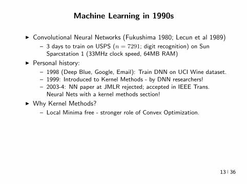
Machine Learning in 1990s
I Convolutional Neural Networks (Fukushima 1980 Lecun et al 1989)
ndash 3 days to train on USPS (n = 7291 digit recognition) on SunSparcstation 1 (33MHz clock speed 64MB RAM)
I Personal history
ndash 1998 (Deep Blue Google Email) Train DNN on UCI Wine datasetndash 1999 Introduced to Kernel Methods - by DNN researchersndash 2003-4 NN paper at JMLR rejected accepted in IEEE Trans
Neural Nets with a kernel methods section
I Why Kernel Methods
ndash Local Minima free - stronger role of Convex Optimization
ndash Theoretically appealingndash Handle non-vectorial data high-dimensional datandash Easier model selection via continuous optimizationndash Matched NN in many cases although didnt scale wrt n as well
I So what changed
ndash More data parallel algorithms hardware Better DNN training
13 36
Machine Learning in 1990s
I Convolutional Neural Networks (Fukushima 1980 Lecun et al 1989)
ndash 3 days to train on USPS (n = 7291 digit recognition) on SunSparcstation 1 (33MHz clock speed 64MB RAM)
I Personal history
ndash 1998 (Deep Blue Google Email) Train DNN on UCI Wine datasetndash 1999 Introduced to Kernel Methods - by DNN researchersndash 2003-4 NN paper at JMLR rejected accepted in IEEE Trans
Neural Nets with a kernel methods section
I Why Kernel Methods
ndash Local Minima free - stronger role of Convex Optimizationndash Theoretically appealing
ndash Handle non-vectorial data high-dimensional datandash Easier model selection via continuous optimizationndash Matched NN in many cases although didnt scale wrt n as well
I So what changed
ndash More data parallel algorithms hardware Better DNN training
13 36
Machine Learning in 1990s
I Convolutional Neural Networks (Fukushima 1980 Lecun et al 1989)
ndash 3 days to train on USPS (n = 7291 digit recognition) on SunSparcstation 1 (33MHz clock speed 64MB RAM)
I Personal history
ndash 1998 (Deep Blue Google Email) Train DNN on UCI Wine datasetndash 1999 Introduced to Kernel Methods - by DNN researchersndash 2003-4 NN paper at JMLR rejected accepted in IEEE Trans
Neural Nets with a kernel methods section
I Why Kernel Methods
ndash Local Minima free - stronger role of Convex Optimizationndash Theoretically appealingndash Handle non-vectorial data high-dimensional datandash Easier model selection via continuous optimization
ndash Matched NN in many cases although didnt scale wrt n as well
I So what changed
ndash More data parallel algorithms hardware Better DNN training
13 36
Machine Learning in 1990s
I Convolutional Neural Networks (Fukushima 1980 Lecun et al 1989)
ndash 3 days to train on USPS (n = 7291 digit recognition) on SunSparcstation 1 (33MHz clock speed 64MB RAM)
I Personal history
ndash 1998 (Deep Blue Google Email) Train DNN on UCI Wine datasetndash 1999 Introduced to Kernel Methods - by DNN researchersndash 2003-4 NN paper at JMLR rejected accepted in IEEE Trans
Neural Nets with a kernel methods section
I Why Kernel Methods
ndash Local Minima free - stronger role of Convex Optimizationndash Theoretically appealingndash Handle non-vectorial data high-dimensional datandash Easier model selection via continuous optimizationndash Matched NN in many cases although didnt scale wrt n as well
I So what changed
ndash More data parallel algorithms hardware Better DNN training
13 36
Machine Learning in 1990s
I Convolutional Neural Networks (Fukushima 1980 Lecun et al 1989)
ndash 3 days to train on USPS (n = 7291 digit recognition) on SunSparcstation 1 (33MHz clock speed 64MB RAM)
I Personal history
ndash 1998 (Deep Blue Google Email) Train DNN on UCI Wine datasetndash 1999 Introduced to Kernel Methods - by DNN researchersndash 2003-4 NN paper at JMLR rejected accepted in IEEE Trans
Neural Nets with a kernel methods section
I Why Kernel Methods
ndash Local Minima free - stronger role of Convex Optimizationndash Theoretically appealingndash Handle non-vectorial data high-dimensional datandash Easier model selection via continuous optimizationndash Matched NN in many cases although didnt scale wrt n as well
I So what changed
ndash More data parallel algorithms hardware Better DNN training
13 36
Kernel Methods vs Neural Networks (Pre-Google)
14 36
Kernel Methods vs Neural Networks
Geoff Hinton facts meme maintained athttpyannlecuncomexfun
I All kernels that ever dared approaching Geoff Hinton woke upconvolved
I The only kernel Geoff Hinton has ever used is a kernel of truth
I If you defy Geoff Hinton he will maximize your entropy in no timeYour free energy will be gone even before you reach equilibrium
Are there synergies between these fields towards design of even better(faster and more accurate) algorithms
15 36
Kernel Methods vs Neural Networks
Geoff Hinton facts meme maintained athttpyannlecuncomexfun
I All kernels that ever dared approaching Geoff Hinton woke upconvolved
I The only kernel Geoff Hinton has ever used is a kernel of truth
I If you defy Geoff Hinton he will maximize your entropy in no timeYour free energy will be gone even before you reach equilibrium
Are there synergies between these fields towards design of even better(faster and more accurate) algorithms
15 36
Kernel Methods vs Neural Networks
Geoff Hinton facts meme maintained athttpyannlecuncomexfun
I All kernels that ever dared approaching Geoff Hinton woke upconvolved
I The only kernel Geoff Hinton has ever used is a kernel of truth
I If you defy Geoff Hinton he will maximize your entropy in no timeYour free energy will be gone even before you reach equilibrium
Are there synergies between these fields towards design of even better(faster and more accurate) algorithms
15 36
Linear Hypotheses
I f(x) = wTxw isin Rn Assume Y sub R setting
arg minwisinRd
lsumi=1
(yi minuswTxi)2 + λw22
w = (XTX + λId)minus1 (XTy
)X =
xTi
isin Rltimesn
I ntimes n linear system =rArr O(ln2 + n3) training time assuming nostructure (eg sparsity)
I O(n) prediction time
I High Approximation error
16 36
Polynomials The expensive way
I Homogeneous degree-d polynomial
f(x) = wTΨnd(x) w isin Rs s =
(d+ nminus 1
d
)
Ψnd(x) =
radic(dα
)xα
isin Rs
α = (α1 αn)sumi
αi = d
(d
α
)=
d
α1 αn
xα = xα11 xα2
2 xαnn
I Construct Z isin Rntimess with rows Ψnd(xi) and solve in O(s3) () time
w = (ZTZ + λId)minus1 (ZTy) (1)
I Note n = 100 d = 4 =rArr s gt 4M
17 36
Polynomials
I Consider the subspace of Rs spanned by the data
S = span (Ψ(x1) Ψ(xl)) = v isin Rs v =
lsumi=1
αiΨ(xi)
I So Rs = S + Sperp Hence for any vector w isin Rs
w = wS + wSperp
I The search of a minimizer can be reduced to S because
lsumi=1
V (wTΨ(xi)) + λw22 gelsumi=1
V (wTSΨ(xi)) + λwS22 + wperpS 22
gelsumi=1
V (wTSΨ(xi)) + λwS22 (2)
I Argument holds for any loss (convex or non-convex additive or not)but needs orthogonality (l2 regularizer) [Representer Theorem]
18 36
Polynomials
I Consider the subspace of Rs spanned by the data
S = span (Ψ(x1) Ψ(xl)) = v isin Rs v =
lsumi=1
αiΨ(xi)
I So Rs = S + Sperp Hence for any vector w isin Rs
w = wS + wSperp
I The search of a minimizer can be reduced to S because
lsumi=1
V (wTΨ(xi)) + λw22 gelsumi=1
V (wTSΨ(xi)) + λwS22 + wperpS 22
gelsumi=1
V (wTSΨ(xi)) + λwS22 (2)
I Argument holds for any loss (convex or non-convex additive or not)but needs orthogonality (l2 regularizer) [Representer Theorem]
18 36
Polynomials
I Consider the subspace of Rs spanned by the data
S = span (Ψ(x1) Ψ(xl)) = v isin Rs v =
lsumi=1
αiΨ(xi)
I So Rs = S + Sperp Hence for any vector w isin Rs
w = wS + wSperp
I The search of a minimizer can be reduced to S because
lsumi=1
V (wTΨ(xi)) + λw22 gelsumi=1
V (wTSΨ(xi)) + λwS22 + wperpS 22
gelsumi=1
V (wTSΨ(xi)) + λwS22 (2)
I Argument holds for any loss (convex or non-convex additive or not)but needs orthogonality (l2 regularizer) [Representer Theorem]
18 36
Polynomials
I Consider the subspace of Rs spanned by the data
S = span (Ψ(x1) Ψ(xl)) = v isin Rs v =
lsumi=1
αiΨ(xi)
I So Rs = S + Sperp Hence for any vector w isin Rs
w = wS + wSperp
I The search of a minimizer can be reduced to S because
lsumi=1
V (wTΨ(xi)) + λw22 gelsumi=1
V (wTSΨ(xi)) + λwS22 + wperpS 22
gelsumi=1
V (wTSΨ(xi)) + λwS22 (2)
I Argument holds for any loss (convex or non-convex additive or not)but needs orthogonality (l2 regularizer) [Representer Theorem]
18 36
Polynomials
I Hence w =sumli=1 βiΨ(xi) isin S for β isin Rl and so we can solve
arg minwisinRd
lsumi=1
(yi minuswTΨ(xi))2 + λw22
arg minβisinRl
lsumj=1
(yj minus
lsumi=1
βiΨ(xi)TΨ(xj)
)2
+ λ
lsumij=1
βiβjΨ(xi)TΨ(xj)
arg minβisinRl
lsumj=1
(yj minus (Gβ)j
)2+ λβTGβ
Gij = Ψ(xi)TΨ(xj)
β = (G + λId)minus1
y
I O(l3 + sl2) training time - O(s3) cost eliminatedI Inference time (O(s) or O(ls))
f(x) = wTΨ(x) =
lsumi=1
βiΨ(xi)TΨ(x)
19 36
Polynomials
I Hence w =sumli=1 βiΨ(xi) isin S for β isin Rl and so we can solve
arg minwisinRd
lsumi=1
(yi minuswTΨ(xi))2 + λw22
arg minβisinRl
lsumj=1
(yj minus
lsumi=1
βiΨ(xi)TΨ(xj)
)2
+ λ
lsumij=1
βiβjΨ(xi)TΨ(xj)
arg minβisinRl
lsumj=1
(yj minus (Gβ)j
)2+ λβTGβ
Gij = Ψ(xi)TΨ(xj)
β = (G + λId)minus1
y
I O(l3 + sl2) training time - O(s3) cost eliminatedI Inference time (O(s) or O(ls))
f(x) = wTΨ(x) =
lsumi=1
βiΨ(xi)TΨ(x)
19 36
Polynomials
I Hence w =sumli=1 βiΨ(xi) isin S for β isin Rl and so we can solve
arg minwisinRd
lsumi=1
(yi minuswTΨ(xi))2 + λw22
arg minβisinRl
lsumj=1
(yj minus
lsumi=1
βiΨ(xi)TΨ(xj)
)2
+ λ
lsumij=1
βiβjΨ(xi)TΨ(xj)
arg minβisinRl
lsumj=1
(yj minus (Gβ)j
)2+ λβTGβ
Gij = Ψ(xi)TΨ(xj)
β = (G + λId)minus1
y
I O(l3 + sl2) training time - O(s3) cost eliminatedI Inference time (O(s) or O(ls))
f(x) = wTΨ(x) =
lsumi=1
βiΨ(xi)TΨ(x)
19 36
Polynomials
I Multinomial Theorem
(z1 + z2 + + zn)d =sum
α|α|=d
(d
α
)zα
I Implicit computation of inner products
Ψ(x)TΨ(xprime) =
ssumi=1
(d
α
)xαxprime
α=
ssumi=1
(d
α
)xα11 xαnn x
primeα11 x
primeαnn
=
ssumi=1
(d
α
)(x1x
prime1)α1(x2x
prime2)α2 (xnx
primen)αn
= (x1xprime1 + xnx
primen)d
= (xTxprime)d
I O(l3 + l2n) training and O(ln) predicting speedI Complexity coming from s has been completely eliminated ()
[Kernel Trick]
20 36
Polynomials
I Multinomial Theorem
(z1 + z2 + + zn)d =sum
α|α|=d
(d
α
)zα
I Implicit computation of inner products
Ψ(x)TΨ(xprime) =
ssumi=1
(d
α
)xαxprime
α=
ssumi=1
(d
α
)xα11 xαnn x
primeα11 x
primeαnn
=
ssumi=1
(d
α
)(x1x
prime1)α1(x2x
prime2)α2 (xnx
primen)αn
= (x1xprime1 + xnx
primen)d
= (xTxprime)d
I O(l3 + l2n) training and O(ln) predicting speedI Complexity coming from s has been completely eliminated ()
[Kernel Trick]
20 36
Polynomials
I Multinomial Theorem
(z1 + z2 + + zn)d =sum
α|α|=d
(d
α
)zα
I Implicit computation of inner products
Ψ(x)TΨ(xprime) =
ssumi=1
(d
α
)xαxprime
α=
ssumi=1
(d
α
)xα11 xαnn x
primeα11 x
primeαnn
=
ssumi=1
(d
α
)(x1x
prime1)α1(x2x
prime2)α2 (xnx
primen)αn
= (x1xprime1 + xnx
primen)d
= (xTxprime)d
I O(l3 + l2n) training and O(ln) predicting speedI Complexity coming from s has been completely eliminated ()
[Kernel Trick]
20 36
Polynomials
I Multinomial Theorem
(z1 + z2 + + zn)d =sum
α|α|=d
(d
α
)zα
I Implicit computation of inner products
Ψ(x)TΨ(xprime) =
ssumi=1
(d
α
)xαxprime
α=
ssumi=1
(d
α
)xα11 xαnn x
primeα11 x
primeαnn
=
ssumi=1
(d
α
)(x1x
prime1)α1(x2x
prime2)α2 (xnx
primen)αn
= (x1xprime1 + xnx
primen)d
= (xTxprime)d
I O(l3 + l2n) training and O(ln) predicting speedI Complexity coming from s has been completely eliminated ()
[Kernel Trick]
20 36
Polynomials
I Multinomial Theorem
(z1 + z2 + + zn)d =sum
α|α|=d
(d
α
)zα
I Implicit computation of inner products
Ψ(x)TΨ(xprime) =
ssumi=1
(d
α
)xαxprime
α=
ssumi=1
(d
α
)xα11 xαnn x
primeα11 x
primeαnn
=
ssumi=1
(d
α
)(x1x
prime1)α1(x2x
prime2)α2 (xnx
primen)αn
= (x1xprime1 + xnx
primen)d
= (xTxprime)d
I O(l3 + l2n) training and O(ln) predicting speedI Complexity coming from s has been completely eliminated ()
[Kernel Trick]
20 36
Polynomials Algorithm
I Algorithm
ndash Start with k X times X 7rarr R k(xxprime) = (xTxprime + 1)d
ndash Construct Gram matrix Gij = k(xixj) on the training samplesndash Solve β = (G + λId)minus1 yndash Return f(x) =
sumli=1 βik(xix)
I f is the optimal degree-d polynomial solving the learning problemin complexity independent of d
I What other forms of k correspond to linear learning inhigh-dimensional nonlinear embeddings of the data
21 36
Polynomials Algorithm
I Algorithm
ndash Start with k X times X 7rarr R k(xxprime) = (xTxprime + 1)d
ndash Construct Gram matrix Gij = k(xixj) on the training samplesndash Solve β = (G + λId)minus1 yndash Return f(x) =
sumli=1 βik(xix)
I f is the optimal degree-d polynomial solving the learning problemin complexity independent of d
I What other forms of k correspond to linear learning inhigh-dimensional nonlinear embeddings of the data
21 36
Symmetric positive semi-definite functions
I Definition A function k X times X 7rarr R is psd if for any finitecollection of points x1 xl the l times l Gram matrix
Gij = k(xixj)
is positive semi-definite ie for any vector β isin Rl
βTGβ =sumij
βiβjk(xixj) ge 0
I Theorem[Mercer] If k is symmetric psd X is compact subset ofRn then it admits an eigenfunction decomposition
k(xxprime) =
Nsumi=1
λiφj(x)φj(xprime) = 〈Ψ(x)Ψ(xprime)〉l2
Ψ(x) = [ radicλjφ(x) ]T (3)
I Feature map associated with a kernel is not uniqueI Functional generalization of positive semi-definite matrices
22 36
Symmetric positive semi-definite functions
I Definition A function k X times X 7rarr R is psd if for any finitecollection of points x1 xl the l times l Gram matrix
Gij = k(xixj)
is positive semi-definite ie for any vector β isin Rl
βTGβ =sumij
βiβjk(xixj) ge 0
I Theorem[Mercer] If k is symmetric psd X is compact subset ofRn then it admits an eigenfunction decomposition
k(xxprime) =
Nsumi=1
λiφj(x)φj(xprime) = 〈Ψ(x)Ψ(xprime)〉l2
Ψ(x) = [ radicλjφ(x) ]T (3)
I Feature map associated with a kernel is not uniqueI Functional generalization of positive semi-definite matrices
22 36
Kernels
I Lineark(xxprime) = xTxprime
I Polynomialk(xxprime) = (xTxprime + 1)d
I Gaussian s =infin Universal
k(xxprime) = eminusxminusxprime2
2σ2
I Conic combinations
k(xxprime) = α1k1(xxprime) + α2k2(xxprime)
I Elementwise products
k(xxprime) = k1(xxprime)k2(xxprime)
I Kernels on discrete sets strings graphs sequences shapes
23 36
Kernels
I Lineark(xxprime) = xTxprime
I Polynomialk(xxprime) = (xTxprime + 1)d
I Gaussian s =infin Universal
k(xxprime) = eminusxminusxprime2
2σ2
I Conic combinations
k(xxprime) = α1k1(xxprime) + α2k2(xxprime)
I Elementwise products
k(xxprime) = k1(xxprime)k2(xxprime)
I Kernels on discrete sets strings graphs sequences shapes
23 36
Kernels
I Lineark(xxprime) = xTxprime
I Polynomialk(xxprime) = (xTxprime + 1)d
I Gaussian s =infin Universal
k(xxprime) = eminusxminusxprime2
2σ2
I Conic combinations
k(xxprime) = α1k1(xxprime) + α2k2(xxprime)
I Elementwise products
k(xxprime) = k1(xxprime)k2(xxprime)
I Kernels on discrete sets strings graphs sequences shapes
23 36
Gaussian Kernel is Positive Definite
I Exponential
eβxTxprime = 1 + βxTxprime +
β2
2(xTy)2 +
β3
3(xTy)3 +
I For any function f Rn 7rarr R psd function k the following kernelis psd
kprime(xxprime) = f(x) (k(xxprime)) f(xprime)
Proofsumij
βiβjkprime(xixj) =
sumij
βiβjf(xi)k(xixj)f(xj) =sumij
βprimeiβprimejk(xixj) ge 0
I Gaussian Kernel
k(xxprime) = eminusxminusxprime22
2σ2
= eminusx222σ2
(e
2xT xprime2σ2
)eminusxprime222σ2 (4)
24 36
Gaussian Kernel is Positive Definite
I Exponential
eβxTxprime = 1 + βxTxprime +
β2
2(xTy)2 +
β3
3(xTy)3 +
I For any function f Rn 7rarr R psd function k the following kernelis psd
kprime(xxprime) = f(x) (k(xxprime)) f(xprime)
Proofsumij
βiβjkprime(xixj) =
sumij
βiβjf(xi)k(xixj)f(xj) =sumij
βprimeiβprimejk(xixj) ge 0
I Gaussian Kernel
k(xxprime) = eminusxminusxprime22
2σ2
= eminusx222σ2
(e
2xT xprime2σ2
)eminusxprime222σ2 (4)
24 36
Gaussian Kernel is Positive Definite
I Exponential
eβxTxprime = 1 + βxTxprime +
β2
2(xTy)2 +
β3
3(xTy)3 +
I For any function f Rn 7rarr R psd function k the following kernelis psd
kprime(xxprime) = f(x) (k(xxprime)) f(xprime)
Proofsumij
βiβjkprime(xixj) =
sumij
βiβjf(xi)k(xixj)f(xj) =sumij
βprimeiβprimejk(xixj) ge 0
I Gaussian Kernel
k(xxprime) = eminusxminusxprime22
2σ2
= eminusx222σ2
(e
2xT xprime2σ2
)eminusxprime222σ2 (4)
24 36
The Mathematical Naturalness of Kernel Methods
I Data X isin Rd Models isin H X 7rarr R
I Geometry in H inner product 〈middot middot〉H norm middot H (Hilbert Spaces)I Theorem All nice Hilbert spaces are generated by a symmetric
positive definite function (the kernel) k(xxprime) on X times XI if f g isin H close ie f minus gH small then f(x) g(x) close forallx isin X I Reproducing Kernel Hilbert Spaces (RKHSs) Hilbert space H
that admit a reproducing kernel ie a function k(xxprime) satisfying
(i) forallx isin X k(middotx) isin H(ii) 〈f k(middotx)〉H = f(x)
I Reproducing kernels are symmetric psdsumij
βiβjk(xixj) = 〈sumi
βik(middotxi)sumi
βik(middotxi)〉H
= sumi
βik(middotxi)2H ge 0 (5)
I (Moore-Aronsjan 1950) Symmetric psd functions arereproducing kernels for some (unique) RKHS Hk
25 36
The Mathematical Naturalness of Kernel Methods
I Data X isin Rd Models isin H X 7rarr RI Geometry in H inner product 〈middot middot〉H norm middot H (Hilbert Spaces)
I Theorem All nice Hilbert spaces are generated by a symmetricpositive definite function (the kernel) k(xxprime) on X times X
I if f g isin H close ie f minus gH small then f(x) g(x) close forallx isin X I Reproducing Kernel Hilbert Spaces (RKHSs) Hilbert space H
that admit a reproducing kernel ie a function k(xxprime) satisfying
(i) forallx isin X k(middotx) isin H(ii) 〈f k(middotx)〉H = f(x)
I Reproducing kernels are symmetric psdsumij
βiβjk(xixj) = 〈sumi
βik(middotxi)sumi
βik(middotxi)〉H
= sumi
βik(middotxi)2H ge 0 (5)
I (Moore-Aronsjan 1950) Symmetric psd functions arereproducing kernels for some (unique) RKHS Hk
25 36
The Mathematical Naturalness of Kernel Methods
I Data X isin Rd Models isin H X 7rarr RI Geometry in H inner product 〈middot middot〉H norm middot H (Hilbert Spaces)I Theorem All nice Hilbert spaces are generated by a symmetric
positive definite function (the kernel) k(xxprime) on X times XI if f g isin H close ie f minus gH small then f(x) g(x) close forallx isin X
I Reproducing Kernel Hilbert Spaces (RKHSs) Hilbert space Hthat admit a reproducing kernel ie a function k(xxprime) satisfying
(i) forallx isin X k(middotx) isin H(ii) 〈f k(middotx)〉H = f(x)
I Reproducing kernels are symmetric psdsumij
βiβjk(xixj) = 〈sumi
βik(middotxi)sumi
βik(middotxi)〉H
= sumi
βik(middotxi)2H ge 0 (5)
I (Moore-Aronsjan 1950) Symmetric psd functions arereproducing kernels for some (unique) RKHS Hk
25 36
The Mathematical Naturalness of Kernel Methods
I Data X isin Rd Models isin H X 7rarr RI Geometry in H inner product 〈middot middot〉H norm middot H (Hilbert Spaces)I Theorem All nice Hilbert spaces are generated by a symmetric
positive definite function (the kernel) k(xxprime) on X times XI if f g isin H close ie f minus gH small then f(x) g(x) close forallx isin X I Reproducing Kernel Hilbert Spaces (RKHSs) Hilbert space H
that admit a reproducing kernel ie a function k(xxprime) satisfying
(i) forallx isin X k(middotx) isin H(ii) 〈f k(middotx)〉H = f(x)
I Reproducing kernels are symmetric psdsumij
βiβjk(xixj) = 〈sumi
βik(middotxi)sumi
βik(middotxi)〉H
= sumi
βik(middotxi)2H ge 0 (5)
I (Moore-Aronsjan 1950) Symmetric psd functions arereproducing kernels for some (unique) RKHS Hk
25 36
The Mathematical Naturalness of Kernel Methods
I Data X isin Rd Models isin H X 7rarr RI Geometry in H inner product 〈middot middot〉H norm middot H (Hilbert Spaces)I Theorem All nice Hilbert spaces are generated by a symmetric
positive definite function (the kernel) k(xxprime) on X times XI if f g isin H close ie f minus gH small then f(x) g(x) close forallx isin X I Reproducing Kernel Hilbert Spaces (RKHSs) Hilbert space H
that admit a reproducing kernel ie a function k(xxprime) satisfying
(i) forallx isin X k(middotx) isin H(ii) 〈f k(middotx)〉H = f(x)
I Reproducing kernels are symmetric psdsumij
βiβjk(xixj) = 〈sumi
βik(middotxi)sumi
βik(middotxi)〉H
= sumi
βik(middotxi)2H ge 0 (5)
I (Moore-Aronsjan 1950) Symmetric psd functions arereproducing kernels for some (unique) RKHS Hk 25 36
Kernel Methods Summary
I Symm pos def function k(x z) on input domain X sub Rd
I k hArr rich Reproducing Kernel Hilbert Space (RKHS) Hk ofreal-valued functions with inner product 〈middot middot〉k and norm middot k
I Regularized Risk Minimization hArr Linear models in an implicithigh-dimensional (often infinite-dimensional) feature space
f = arg minfisinHk
1
n
nsumi=1
V (yi f(xi)) + λf2Hk xi isin Rd
I Representer Theorem f(x) =sumni=1 αik(xxi)
26 36
Shallow and Deep Function Spaces
I What does it mean to understand a function space
ndash Linear f(x) = wTxw isin Rd
ndash Polynomial f(x) = wT Ψ(x)w isin Rs
ndash RKHS balls f isin Hk fk lt γ [like vM le 1]
I Shallow nets f(x) = wTσ(Wx) (w isin RdW isin Rs)ndash For srarrinfin W sim p σ(u) = eminusiu approximates Gaussian kernel
methodsndash Theorem [Bochner 1937] One-to-one correspondence between k
and a density p such that
k(x z) = ψ(xminus z) =
intRdeminusi(xminusz)Twp(w)dw asymp 1
s
ssumj=1
eminusi(xminusz)Twj
Gaussian kernel k(x z) = eminusxminusz22
2σ2 lArrrArr p = N (0 σminus2Id)ndash Similar integral approx relates ReLU to the arc-cosine kernelndash Optimization versus Randomization
27 36
Shallow and Deep Function Spaces
I What does it mean to understand a function space
ndash Linear f(x) = wTxw isin Rd
ndash Polynomial f(x) = wT Ψ(x)w isin Rs
ndash RKHS balls f isin Hk fk lt γ [like vM le 1]
I Shallow nets f(x) = wTσ(Wx) (w isin RdW isin Rs)ndash For srarrinfin W sim p σ(u) = eminusiu approximates Gaussian kernel
methodsndash Theorem [Bochner 1937] One-to-one correspondence between k
and a density p such that
k(x z) = ψ(xminus z) =
intRdeminusi(xminusz)Twp(w)dw asymp 1
s
ssumj=1
eminusi(xminusz)Twj
Gaussian kernel k(x z) = eminusxminusz22
2σ2 lArrrArr p = N (0 σminus2Id)ndash Similar integral approx relates ReLU to the arc-cosine kernelndash Optimization versus Randomization
27 36
Shallow and Deep Function Spaces
I What does it mean to understand a function space
ndash Linear f(x) = wTxw isin Rd
ndash Polynomial f(x) = wT Ψ(x)w isin Rs
ndash RKHS balls f isin Hk fk lt γ [like vM le 1]
I Shallow nets f(x) = wTσ(Wx) (w isin RdW isin Rs)ndash For srarrinfin W sim p σ(u) = eminusiu approximates Gaussian kernel
methodsndash Theorem [Bochner 1937] One-to-one correspondence between k
and a density p such that
k(x z) = ψ(xminus z) =
intRdeminusi(xminusz)Twp(w)dw asymp 1
s
ssumj=1
eminusi(xminusz)Twj
Gaussian kernel k(x z) = eminusxminusz22
2σ2 lArrrArr p = N (0 σminus2Id)ndash Similar integral approx relates ReLU to the arc-cosine kernelndash Optimization versus Randomization
27 36
Shallow and Deep Function Spaces
I What does it mean to understand a function space
ndash Linear f(x) = wTxw isin Rd
ndash Polynomial f(x) = wT Ψ(x)w isin Rs
ndash RKHS balls f isin Hk fk lt γ [like vM le 1]
I Shallow nets f(x) = wTσ(Wx) (w isin RdW isin Rs)
ndash For srarrinfin W sim p σ(u) = eminusiu approximates Gaussian kernelmethods
ndash Theorem [Bochner 1937] One-to-one correspondence between kand a density p such that
k(x z) = ψ(xminus z) =
intRdeminusi(xminusz)Twp(w)dw asymp 1
s
ssumj=1
eminusi(xminusz)Twj
Gaussian kernel k(x z) = eminusxminusz22
2σ2 lArrrArr p = N (0 σminus2Id)ndash Similar integral approx relates ReLU to the arc-cosine kernelndash Optimization versus Randomization
27 36
Shallow and Deep Function Spaces
I What does it mean to understand a function space
ndash Linear f(x) = wTxw isin Rd
ndash Polynomial f(x) = wT Ψ(x)w isin Rs
ndash RKHS balls f isin Hk fk lt γ [like vM le 1]
I Shallow nets f(x) = wTσ(Wx) (w isin RdW isin Rs)ndash For srarrinfin W sim p σ(u) = eminusiu approximates Gaussian kernel
methodsndash Theorem [Bochner 1937] One-to-one correspondence between k
and a density p such that
k(x z) = ψ(xminus z) =
intRdeminusi(xminusz)Twp(w)dw asymp 1
s
ssumj=1
eminusi(xminusz)Twj
Gaussian kernel k(x z) = eminusxminusz22
2σ2 lArrrArr p = N (0 σminus2Id)ndash Similar integral approx relates ReLU to the arc-cosine kernelndash Optimization versus Randomization
27 36
Expressivity of Deep Nets Linear Regions
I The ReLU map f(x) = max(Wx 0)W isin Rwtimesn is piecewise linear
I A piece is a connected region (a convex polytope) of Rd with sharedsparsity pattern in activations
I (Zaslavsky 1975) Number of linear regions formed by an arrangement of
s hyperplanes in d-dimensions in general position issumd
i=0
(si
)I Composition of ReLU maps is also piecewise linear
I (Raghu et al 2017 Pascano et al 2014 Montufar 2014) Number oflinear regions grows as O(wnd) for a composition of d ReLU maps(nrarr brarr brarr b rarr b) each of width w
I (Safran and Shamir 2017)
ndash 1[x le 1] x isin Rd ε-accurate 3-layer network with O(dε) neurons but cannot be approximated with
accuracy higher than O(1d4) using 2-layer networks unless width is exponential in d
28 36
Expressivity of Deep Nets Linear Regions
I The ReLU map f(x) = max(Wx 0)W isin Rwtimesn is piecewise linear
I A piece is a connected region (a convex polytope) of Rd with sharedsparsity pattern in activations
I (Zaslavsky 1975) Number of linear regions formed by an arrangement of
s hyperplanes in d-dimensions in general position issumd
i=0
(si
)I Composition of ReLU maps is also piecewise linear
I (Raghu et al 2017 Pascano et al 2014 Montufar 2014) Number oflinear regions grows as O(wnd) for a composition of d ReLU maps(nrarr brarr brarr b rarr b) each of width w
I (Safran and Shamir 2017)
ndash 1[x le 1] x isin Rd ε-accurate 3-layer network with O(dε) neurons but cannot be approximated with
accuracy higher than O(1d4) using 2-layer networks unless width is exponential in d
28 36
Expressivity of Deep Nets Linear Regions
I The ReLU map f(x) = max(Wx 0)W isin Rwtimesn is piecewise linear
I A piece is a connected region (a convex polytope) of Rd with sharedsparsity pattern in activations
I (Zaslavsky 1975) Number of linear regions formed by an arrangement of
s hyperplanes in d-dimensions in general position issumd
i=0
(si
)
I Composition of ReLU maps is also piecewise linear
I (Raghu et al 2017 Pascano et al 2014 Montufar 2014) Number oflinear regions grows as O(wnd) for a composition of d ReLU maps(nrarr brarr brarr b rarr b) each of width w
I (Safran and Shamir 2017)
ndash 1[x le 1] x isin Rd ε-accurate 3-layer network with O(dε) neurons but cannot be approximated with
accuracy higher than O(1d4) using 2-layer networks unless width is exponential in d
28 36
Expressivity of Deep Nets Linear Regions
I The ReLU map f(x) = max(Wx 0)W isin Rwtimesn is piecewise linear
I A piece is a connected region (a convex polytope) of Rd with sharedsparsity pattern in activations
I (Zaslavsky 1975) Number of linear regions formed by an arrangement of
s hyperplanes in d-dimensions in general position issumd
i=0
(si
)I Composition of ReLU maps is also piecewise linear
I (Raghu et al 2017 Pascano et al 2014 Montufar 2014) Number oflinear regions grows as O(wnd) for a composition of d ReLU maps(nrarr brarr brarr b rarr b) each of width w
I (Safran and Shamir 2017)
ndash 1[x le 1] x isin Rd ε-accurate 3-layer network with O(dε) neurons but cannot be approximated with
accuracy higher than O(1d4) using 2-layer networks unless width is exponential in d28 36
Expressivity of Deep Nets Trajectory Length
I (Raghu et al 2017) Trajectory Length (ldquogeneralized operator normrdquo)How much is a curve in the input space stretched by a layer in thenetwork
29 36
Expressivity of Deep Nets Trajectory Length
I (Raghu et al 2017) Trajectory Length (ldquogeneralized operator normrdquo)How much is a curve in the input space stretched by a layer in thenetwork
29 36
Expressivity and Generalization
I Expressiveness equiv capacity to fit random noise =rArr susceptibility tooverfitting (VC dimension Rademacher Complexity)
I Zhang et al 2017 Famous CNNs easily fit random labels
ndash Over-parameterized (n=12M psim 60M) but structuredndash Domain-knowledge baked in does not constraint expressiveness
I CNNs tend to generalize even without regularization (explicit and implicit)
I For linear regression SGD returns minimum norm solution
30 36
Expressivity and Generalization
I Expressiveness equiv capacity to fit random noise =rArr susceptibility tooverfitting (VC dimension Rademacher Complexity)
I Zhang et al 2017 Famous CNNs easily fit random labels
ndash Over-parameterized (n=12M psim 60M) but structuredndash Domain-knowledge baked in does not constraint expressiveness
I CNNs tend to generalize even without regularization (explicit and implicit)
I For linear regression SGD returns minimum norm solution
30 36
Expressivity and Generalization
I Expressiveness equiv capacity to fit random noise =rArr susceptibility tooverfitting (VC dimension Rademacher Complexity)
I Zhang et al 2017 Famous CNNs easily fit random labels
ndash Over-parameterized (n=12M psim 60M) but structuredndash Domain-knowledge baked in does not constraint expressiveness
I CNNs tend to generalize even without regularization (explicit and implicit)
I For linear regression SGD returns minimum norm solution
30 36
Optimization Landscape Symmetry and Saddle Points
I Folklore lots of equivalent good local minI Classification of critical points based on Hessian spectrumI Permutation and Scaling symmetries
I Thm [Lee et al 2016 Anadkumar Ge] For the short-step gradientmethod the basin of attraction of strict saddle points (atleast onenegative eigenvalue) has measure zero
31 36
Optimization Landscape Symmetry and Saddle Points
I Folklore lots of equivalent good local minI Classification of critical points based on Hessian spectrumI Permutation and Scaling symmetries
I Thm [Lee et al 2016 Anadkumar Ge] For the short-step gradientmethod the basin of attraction of strict saddle points (atleast onenegative eigenvalue) has measure zero
31 36
Optimization Landscape Symmetry and Saddle Points
I Folklore lots of equivalent good local minI Classification of critical points based on Hessian spectrumI Permutation and Scaling symmetries
I Thm [Lee et al 2016 Anadkumar Ge] For the short-step gradientmethod the basin of attraction of strict saddle points (atleast onenegative eigenvalue) has measure zero
31 36
Optimization Landscape Sharp Minima and Stability
Keskar et al 2017 On large-batch training for DL Generalization Gap and Sharp Minima
32 36
Deep Learning Computational Graphs TensorFlow
tensorfloworg
I Tensors-in Tensors-out
I Evergrowing list of Tensor-Ops (PythonC++)
f(xw)
[partf
partx
]T v
[partf
partw
]T v
I Automatic Differentiation Reverse mode
partxL
partxi=sumirarrj
partxL
partxj
partxj
partxi
33 36
Computational Graphs and TensorFlow
tensorfloworg
I SGD with minibatches
wk+1 = wk minus ηlsumi=1
partli
partw
∣∣∣wt
I Model Parallelism Assign independent paths tothreads GPUs
I Data Parallelism create Graph replicas on differentmachines
I Mobile TensorFlow
34 36
Computational Graphs and TensorFlow
tensorfloworg
35 36
Computational Graphs and TensorFlow
tensorfloworg
35 36
Computational Graphs and TensorFlow
tensorfloworg
35 36
Challenges and Opportunities
I Lots of fascinating unsolved problems
I Can you win Imagenet with Convex optimization
I Tools from polynomial optimization (global optimization deep-RL)
I Supervised to Semi-supervised to Unsupervised Learning
I Compact efficient real-time models (eliminateover-parametrization) for new form factors
I Exciting emerging world of Robotics Wearable ComputersIntelligent home devices Personal digital assistants
Google Internship Program
36 36
- anm0
- fdrm0
- fdrm5
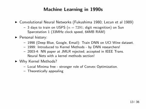
Machine Learning in 1990s
I Convolutional Neural Networks (Fukushima 1980 Lecun et al 1989)
ndash 3 days to train on USPS (n = 7291 digit recognition) on SunSparcstation 1 (33MHz clock speed 64MB RAM)
I Personal history
ndash 1998 (Deep Blue Google Email) Train DNN on UCI Wine datasetndash 1999 Introduced to Kernel Methods - by DNN researchersndash 2003-4 NN paper at JMLR rejected accepted in IEEE Trans
Neural Nets with a kernel methods section
I Why Kernel Methods
ndash Local Minima free - stronger role of Convex Optimizationndash Theoretically appealingndash Handle non-vectorial data high-dimensional datandash Easier model selection via continuous optimizationndash Matched NN in many cases although didnt scale wrt n as well
I So what changed
ndash More data parallel algorithms hardware Better DNN training
13 36
Kernel Methods vs Neural Networks (Pre-Google)
14 36
Kernel Methods vs Neural Networks
Geoff Hinton facts meme maintained athttpyannlecuncomexfun
I All kernels that ever dared approaching Geoff Hinton woke upconvolved
I The only kernel Geoff Hinton has ever used is a kernel of truth
I If you defy Geoff Hinton he will maximize your entropy in no timeYour free energy will be gone even before you reach equilibrium
Are there synergies between these fields towards design of even better(faster and more accurate) algorithms
15 36
Kernel Methods vs Neural Networks
Geoff Hinton facts meme maintained athttpyannlecuncomexfun
I All kernels that ever dared approaching Geoff Hinton woke upconvolved
I The only kernel Geoff Hinton has ever used is a kernel of truth
I If you defy Geoff Hinton he will maximize your entropy in no timeYour free energy will be gone even before you reach equilibrium
Are there synergies between these fields towards design of even better(faster and more accurate) algorithms
15 36
Kernel Methods vs Neural Networks
Geoff Hinton facts meme maintained athttpyannlecuncomexfun
I All kernels that ever dared approaching Geoff Hinton woke upconvolved
I The only kernel Geoff Hinton has ever used is a kernel of truth
I If you defy Geoff Hinton he will maximize your entropy in no timeYour free energy will be gone even before you reach equilibrium
Are there synergies between these fields towards design of even better(faster and more accurate) algorithms
15 36
Linear Hypotheses
I f(x) = wTxw isin Rn Assume Y sub R setting
arg minwisinRd
lsumi=1
(yi minuswTxi)2 + λw22
w = (XTX + λId)minus1 (XTy
)X =
xTi
isin Rltimesn
I ntimes n linear system =rArr O(ln2 + n3) training time assuming nostructure (eg sparsity)
I O(n) prediction time
I High Approximation error
16 36
Polynomials The expensive way
I Homogeneous degree-d polynomial
f(x) = wTΨnd(x) w isin Rs s =
(d+ nminus 1
d
)
Ψnd(x) =
radic(dα
)xα
isin Rs
α = (α1 αn)sumi
αi = d
(d
α
)=
d
α1 αn
xα = xα11 xα2
2 xαnn
I Construct Z isin Rntimess with rows Ψnd(xi) and solve in O(s3) () time
w = (ZTZ + λId)minus1 (ZTy) (1)
I Note n = 100 d = 4 =rArr s gt 4M
17 36
Polynomials
I Consider the subspace of Rs spanned by the data
S = span (Ψ(x1) Ψ(xl)) = v isin Rs v =
lsumi=1
αiΨ(xi)
I So Rs = S + Sperp Hence for any vector w isin Rs
w = wS + wSperp
I The search of a minimizer can be reduced to S because
lsumi=1
V (wTΨ(xi)) + λw22 gelsumi=1
V (wTSΨ(xi)) + λwS22 + wperpS 22
gelsumi=1
V (wTSΨ(xi)) + λwS22 (2)
I Argument holds for any loss (convex or non-convex additive or not)but needs orthogonality (l2 regularizer) [Representer Theorem]
18 36
Polynomials
I Consider the subspace of Rs spanned by the data
S = span (Ψ(x1) Ψ(xl)) = v isin Rs v =
lsumi=1
αiΨ(xi)
I So Rs = S + Sperp Hence for any vector w isin Rs
w = wS + wSperp
I The search of a minimizer can be reduced to S because
lsumi=1
V (wTΨ(xi)) + λw22 gelsumi=1
V (wTSΨ(xi)) + λwS22 + wperpS 22
gelsumi=1
V (wTSΨ(xi)) + λwS22 (2)
I Argument holds for any loss (convex or non-convex additive or not)but needs orthogonality (l2 regularizer) [Representer Theorem]
18 36
Polynomials
I Consider the subspace of Rs spanned by the data
S = span (Ψ(x1) Ψ(xl)) = v isin Rs v =
lsumi=1
αiΨ(xi)
I So Rs = S + Sperp Hence for any vector w isin Rs
w = wS + wSperp
I The search of a minimizer can be reduced to S because
lsumi=1
V (wTΨ(xi)) + λw22 gelsumi=1
V (wTSΨ(xi)) + λwS22 + wperpS 22
gelsumi=1
V (wTSΨ(xi)) + λwS22 (2)
I Argument holds for any loss (convex or non-convex additive or not)but needs orthogonality (l2 regularizer) [Representer Theorem]
18 36
Polynomials
I Consider the subspace of Rs spanned by the data
S = span (Ψ(x1) Ψ(xl)) = v isin Rs v =
lsumi=1
αiΨ(xi)
I So Rs = S + Sperp Hence for any vector w isin Rs
w = wS + wSperp
I The search of a minimizer can be reduced to S because
lsumi=1
V (wTΨ(xi)) + λw22 gelsumi=1
V (wTSΨ(xi)) + λwS22 + wperpS 22
gelsumi=1
V (wTSΨ(xi)) + λwS22 (2)
I Argument holds for any loss (convex or non-convex additive or not)but needs orthogonality (l2 regularizer) [Representer Theorem]
18 36
Polynomials
I Hence w =sumli=1 βiΨ(xi) isin S for β isin Rl and so we can solve
arg minwisinRd
lsumi=1
(yi minuswTΨ(xi))2 + λw22
arg minβisinRl
lsumj=1
(yj minus
lsumi=1
βiΨ(xi)TΨ(xj)
)2
+ λ
lsumij=1
βiβjΨ(xi)TΨ(xj)
arg minβisinRl
lsumj=1
(yj minus (Gβ)j
)2+ λβTGβ
Gij = Ψ(xi)TΨ(xj)
β = (G + λId)minus1
y
I O(l3 + sl2) training time - O(s3) cost eliminatedI Inference time (O(s) or O(ls))
f(x) = wTΨ(x) =
lsumi=1
βiΨ(xi)TΨ(x)
19 36
Polynomials
I Hence w =sumli=1 βiΨ(xi) isin S for β isin Rl and so we can solve
arg minwisinRd
lsumi=1
(yi minuswTΨ(xi))2 + λw22
arg minβisinRl
lsumj=1
(yj minus
lsumi=1
βiΨ(xi)TΨ(xj)
)2
+ λ
lsumij=1
βiβjΨ(xi)TΨ(xj)
arg minβisinRl
lsumj=1
(yj minus (Gβ)j
)2+ λβTGβ
Gij = Ψ(xi)TΨ(xj)
β = (G + λId)minus1
y
I O(l3 + sl2) training time - O(s3) cost eliminatedI Inference time (O(s) or O(ls))
f(x) = wTΨ(x) =
lsumi=1
βiΨ(xi)TΨ(x)
19 36
Polynomials
I Hence w =sumli=1 βiΨ(xi) isin S for β isin Rl and so we can solve
arg minwisinRd
lsumi=1
(yi minuswTΨ(xi))2 + λw22
arg minβisinRl
lsumj=1
(yj minus
lsumi=1
βiΨ(xi)TΨ(xj)
)2
+ λ
lsumij=1
βiβjΨ(xi)TΨ(xj)
arg minβisinRl
lsumj=1
(yj minus (Gβ)j
)2+ λβTGβ
Gij = Ψ(xi)TΨ(xj)
β = (G + λId)minus1
y
I O(l3 + sl2) training time - O(s3) cost eliminatedI Inference time (O(s) or O(ls))
f(x) = wTΨ(x) =
lsumi=1
βiΨ(xi)TΨ(x)
19 36
Polynomials
I Multinomial Theorem
(z1 + z2 + + zn)d =sum
α|α|=d
(d
α
)zα
I Implicit computation of inner products
Ψ(x)TΨ(xprime) =
ssumi=1
(d
α
)xαxprime
α=
ssumi=1
(d
α
)xα11 xαnn x
primeα11 x
primeαnn
=
ssumi=1
(d
α
)(x1x
prime1)α1(x2x
prime2)α2 (xnx
primen)αn
= (x1xprime1 + xnx
primen)d
= (xTxprime)d
I O(l3 + l2n) training and O(ln) predicting speedI Complexity coming from s has been completely eliminated ()
[Kernel Trick]
20 36
Polynomials
I Multinomial Theorem
(z1 + z2 + + zn)d =sum
α|α|=d
(d
α
)zα
I Implicit computation of inner products
Ψ(x)TΨ(xprime) =
ssumi=1
(d
α
)xαxprime
α=
ssumi=1
(d
α
)xα11 xαnn x
primeα11 x
primeαnn
=
ssumi=1
(d
α
)(x1x
prime1)α1(x2x
prime2)α2 (xnx
primen)αn
= (x1xprime1 + xnx
primen)d
= (xTxprime)d
I O(l3 + l2n) training and O(ln) predicting speedI Complexity coming from s has been completely eliminated ()
[Kernel Trick]
20 36
Polynomials
I Multinomial Theorem
(z1 + z2 + + zn)d =sum
α|α|=d
(d
α
)zα
I Implicit computation of inner products
Ψ(x)TΨ(xprime) =
ssumi=1
(d
α
)xαxprime
α=
ssumi=1
(d
α
)xα11 xαnn x
primeα11 x
primeαnn
=
ssumi=1
(d
α
)(x1x
prime1)α1(x2x
prime2)α2 (xnx
primen)αn
= (x1xprime1 + xnx
primen)d
= (xTxprime)d
I O(l3 + l2n) training and O(ln) predicting speedI Complexity coming from s has been completely eliminated ()
[Kernel Trick]
20 36
Polynomials
I Multinomial Theorem
(z1 + z2 + + zn)d =sum
α|α|=d
(d
α
)zα
I Implicit computation of inner products
Ψ(x)TΨ(xprime) =
ssumi=1
(d
α
)xαxprime
α=
ssumi=1
(d
α
)xα11 xαnn x
primeα11 x
primeαnn
=
ssumi=1
(d
α
)(x1x
prime1)α1(x2x
prime2)α2 (xnx
primen)αn
= (x1xprime1 + xnx
primen)d
= (xTxprime)d
I O(l3 + l2n) training and O(ln) predicting speedI Complexity coming from s has been completely eliminated ()
[Kernel Trick]
20 36
Polynomials
I Multinomial Theorem
(z1 + z2 + + zn)d =sum
α|α|=d
(d
α
)zα
I Implicit computation of inner products
Ψ(x)TΨ(xprime) =
ssumi=1
(d
α
)xαxprime
α=
ssumi=1
(d
α
)xα11 xαnn x
primeα11 x
primeαnn
=
ssumi=1
(d
α
)(x1x
prime1)α1(x2x
prime2)α2 (xnx
primen)αn
= (x1xprime1 + xnx
primen)d
= (xTxprime)d
I O(l3 + l2n) training and O(ln) predicting speedI Complexity coming from s has been completely eliminated ()
[Kernel Trick]
20 36
Polynomials Algorithm
I Algorithm
ndash Start with k X times X 7rarr R k(xxprime) = (xTxprime + 1)d
ndash Construct Gram matrix Gij = k(xixj) on the training samplesndash Solve β = (G + λId)minus1 yndash Return f(x) =
sumli=1 βik(xix)
I f is the optimal degree-d polynomial solving the learning problemin complexity independent of d
I What other forms of k correspond to linear learning inhigh-dimensional nonlinear embeddings of the data
21 36
Polynomials Algorithm
I Algorithm
ndash Start with k X times X 7rarr R k(xxprime) = (xTxprime + 1)d
ndash Construct Gram matrix Gij = k(xixj) on the training samplesndash Solve β = (G + λId)minus1 yndash Return f(x) =
sumli=1 βik(xix)
I f is the optimal degree-d polynomial solving the learning problemin complexity independent of d
I What other forms of k correspond to linear learning inhigh-dimensional nonlinear embeddings of the data
21 36
Symmetric positive semi-definite functions
I Definition A function k X times X 7rarr R is psd if for any finitecollection of points x1 xl the l times l Gram matrix
Gij = k(xixj)
is positive semi-definite ie for any vector β isin Rl
βTGβ =sumij
βiβjk(xixj) ge 0
I Theorem[Mercer] If k is symmetric psd X is compact subset ofRn then it admits an eigenfunction decomposition
k(xxprime) =
Nsumi=1
λiφj(x)φj(xprime) = 〈Ψ(x)Ψ(xprime)〉l2
Ψ(x) = [ radicλjφ(x) ]T (3)
I Feature map associated with a kernel is not uniqueI Functional generalization of positive semi-definite matrices
22 36
Symmetric positive semi-definite functions
I Definition A function k X times X 7rarr R is psd if for any finitecollection of points x1 xl the l times l Gram matrix
Gij = k(xixj)
is positive semi-definite ie for any vector β isin Rl
βTGβ =sumij
βiβjk(xixj) ge 0
I Theorem[Mercer] If k is symmetric psd X is compact subset ofRn then it admits an eigenfunction decomposition
k(xxprime) =
Nsumi=1
λiφj(x)φj(xprime) = 〈Ψ(x)Ψ(xprime)〉l2
Ψ(x) = [ radicλjφ(x) ]T (3)
I Feature map associated with a kernel is not uniqueI Functional generalization of positive semi-definite matrices
22 36
Kernels
I Lineark(xxprime) = xTxprime
I Polynomialk(xxprime) = (xTxprime + 1)d
I Gaussian s =infin Universal
k(xxprime) = eminusxminusxprime2
2σ2
I Conic combinations
k(xxprime) = α1k1(xxprime) + α2k2(xxprime)
I Elementwise products
k(xxprime) = k1(xxprime)k2(xxprime)
I Kernels on discrete sets strings graphs sequences shapes
23 36
Kernels
I Lineark(xxprime) = xTxprime
I Polynomialk(xxprime) = (xTxprime + 1)d
I Gaussian s =infin Universal
k(xxprime) = eminusxminusxprime2
2σ2
I Conic combinations
k(xxprime) = α1k1(xxprime) + α2k2(xxprime)
I Elementwise products
k(xxprime) = k1(xxprime)k2(xxprime)
I Kernels on discrete sets strings graphs sequences shapes
23 36
Kernels
I Lineark(xxprime) = xTxprime
I Polynomialk(xxprime) = (xTxprime + 1)d
I Gaussian s =infin Universal
k(xxprime) = eminusxminusxprime2
2σ2
I Conic combinations
k(xxprime) = α1k1(xxprime) + α2k2(xxprime)
I Elementwise products
k(xxprime) = k1(xxprime)k2(xxprime)
I Kernels on discrete sets strings graphs sequences shapes
23 36
Gaussian Kernel is Positive Definite
I Exponential
eβxTxprime = 1 + βxTxprime +
β2
2(xTy)2 +
β3
3(xTy)3 +
I For any function f Rn 7rarr R psd function k the following kernelis psd
kprime(xxprime) = f(x) (k(xxprime)) f(xprime)
Proofsumij
βiβjkprime(xixj) =
sumij
βiβjf(xi)k(xixj)f(xj) =sumij
βprimeiβprimejk(xixj) ge 0
I Gaussian Kernel
k(xxprime) = eminusxminusxprime22
2σ2
= eminusx222σ2
(e
2xT xprime2σ2
)eminusxprime222σ2 (4)
24 36
Gaussian Kernel is Positive Definite
I Exponential
eβxTxprime = 1 + βxTxprime +
β2
2(xTy)2 +
β3
3(xTy)3 +
I For any function f Rn 7rarr R psd function k the following kernelis psd
kprime(xxprime) = f(x) (k(xxprime)) f(xprime)
Proofsumij
βiβjkprime(xixj) =
sumij
βiβjf(xi)k(xixj)f(xj) =sumij
βprimeiβprimejk(xixj) ge 0
I Gaussian Kernel
k(xxprime) = eminusxminusxprime22
2σ2
= eminusx222σ2
(e
2xT xprime2σ2
)eminusxprime222σ2 (4)
24 36
Gaussian Kernel is Positive Definite
I Exponential
eβxTxprime = 1 + βxTxprime +
β2
2(xTy)2 +
β3
3(xTy)3 +
I For any function f Rn 7rarr R psd function k the following kernelis psd
kprime(xxprime) = f(x) (k(xxprime)) f(xprime)
Proofsumij
βiβjkprime(xixj) =
sumij
βiβjf(xi)k(xixj)f(xj) =sumij
βprimeiβprimejk(xixj) ge 0
I Gaussian Kernel
k(xxprime) = eminusxminusxprime22
2σ2
= eminusx222σ2
(e
2xT xprime2σ2
)eminusxprime222σ2 (4)
24 36
The Mathematical Naturalness of Kernel Methods
I Data X isin Rd Models isin H X 7rarr R
I Geometry in H inner product 〈middot middot〉H norm middot H (Hilbert Spaces)I Theorem All nice Hilbert spaces are generated by a symmetric
positive definite function (the kernel) k(xxprime) on X times XI if f g isin H close ie f minus gH small then f(x) g(x) close forallx isin X I Reproducing Kernel Hilbert Spaces (RKHSs) Hilbert space H
that admit a reproducing kernel ie a function k(xxprime) satisfying
(i) forallx isin X k(middotx) isin H(ii) 〈f k(middotx)〉H = f(x)
I Reproducing kernels are symmetric psdsumij
βiβjk(xixj) = 〈sumi
βik(middotxi)sumi
βik(middotxi)〉H
= sumi
βik(middotxi)2H ge 0 (5)
I (Moore-Aronsjan 1950) Symmetric psd functions arereproducing kernels for some (unique) RKHS Hk
25 36
The Mathematical Naturalness of Kernel Methods
I Data X isin Rd Models isin H X 7rarr RI Geometry in H inner product 〈middot middot〉H norm middot H (Hilbert Spaces)
I Theorem All nice Hilbert spaces are generated by a symmetricpositive definite function (the kernel) k(xxprime) on X times X
I if f g isin H close ie f minus gH small then f(x) g(x) close forallx isin X I Reproducing Kernel Hilbert Spaces (RKHSs) Hilbert space H
that admit a reproducing kernel ie a function k(xxprime) satisfying
(i) forallx isin X k(middotx) isin H(ii) 〈f k(middotx)〉H = f(x)
I Reproducing kernels are symmetric psdsumij
βiβjk(xixj) = 〈sumi
βik(middotxi)sumi
βik(middotxi)〉H
= sumi
βik(middotxi)2H ge 0 (5)
I (Moore-Aronsjan 1950) Symmetric psd functions arereproducing kernels for some (unique) RKHS Hk
25 36
The Mathematical Naturalness of Kernel Methods
I Data X isin Rd Models isin H X 7rarr RI Geometry in H inner product 〈middot middot〉H norm middot H (Hilbert Spaces)I Theorem All nice Hilbert spaces are generated by a symmetric
positive definite function (the kernel) k(xxprime) on X times XI if f g isin H close ie f minus gH small then f(x) g(x) close forallx isin X
I Reproducing Kernel Hilbert Spaces (RKHSs) Hilbert space Hthat admit a reproducing kernel ie a function k(xxprime) satisfying
(i) forallx isin X k(middotx) isin H(ii) 〈f k(middotx)〉H = f(x)
I Reproducing kernels are symmetric psdsumij
βiβjk(xixj) = 〈sumi
βik(middotxi)sumi
βik(middotxi)〉H
= sumi
βik(middotxi)2H ge 0 (5)
I (Moore-Aronsjan 1950) Symmetric psd functions arereproducing kernels for some (unique) RKHS Hk
25 36
The Mathematical Naturalness of Kernel Methods
I Data X isin Rd Models isin H X 7rarr RI Geometry in H inner product 〈middot middot〉H norm middot H (Hilbert Spaces)I Theorem All nice Hilbert spaces are generated by a symmetric
positive definite function (the kernel) k(xxprime) on X times XI if f g isin H close ie f minus gH small then f(x) g(x) close forallx isin X I Reproducing Kernel Hilbert Spaces (RKHSs) Hilbert space H
that admit a reproducing kernel ie a function k(xxprime) satisfying
(i) forallx isin X k(middotx) isin H(ii) 〈f k(middotx)〉H = f(x)
I Reproducing kernels are symmetric psdsumij
βiβjk(xixj) = 〈sumi
βik(middotxi)sumi
βik(middotxi)〉H
= sumi
βik(middotxi)2H ge 0 (5)
I (Moore-Aronsjan 1950) Symmetric psd functions arereproducing kernels for some (unique) RKHS Hk
25 36
The Mathematical Naturalness of Kernel Methods
I Data X isin Rd Models isin H X 7rarr RI Geometry in H inner product 〈middot middot〉H norm middot H (Hilbert Spaces)I Theorem All nice Hilbert spaces are generated by a symmetric
positive definite function (the kernel) k(xxprime) on X times XI if f g isin H close ie f minus gH small then f(x) g(x) close forallx isin X I Reproducing Kernel Hilbert Spaces (RKHSs) Hilbert space H
that admit a reproducing kernel ie a function k(xxprime) satisfying
(i) forallx isin X k(middotx) isin H(ii) 〈f k(middotx)〉H = f(x)
I Reproducing kernels are symmetric psdsumij
βiβjk(xixj) = 〈sumi
βik(middotxi)sumi
βik(middotxi)〉H
= sumi
βik(middotxi)2H ge 0 (5)
I (Moore-Aronsjan 1950) Symmetric psd functions arereproducing kernels for some (unique) RKHS Hk 25 36
Kernel Methods Summary
I Symm pos def function k(x z) on input domain X sub Rd
I k hArr rich Reproducing Kernel Hilbert Space (RKHS) Hk ofreal-valued functions with inner product 〈middot middot〉k and norm middot k
I Regularized Risk Minimization hArr Linear models in an implicithigh-dimensional (often infinite-dimensional) feature space
f = arg minfisinHk
1
n
nsumi=1
V (yi f(xi)) + λf2Hk xi isin Rd
I Representer Theorem f(x) =sumni=1 αik(xxi)
26 36
Shallow and Deep Function Spaces
I What does it mean to understand a function space
ndash Linear f(x) = wTxw isin Rd
ndash Polynomial f(x) = wT Ψ(x)w isin Rs
ndash RKHS balls f isin Hk fk lt γ [like vM le 1]
I Shallow nets f(x) = wTσ(Wx) (w isin RdW isin Rs)ndash For srarrinfin W sim p σ(u) = eminusiu approximates Gaussian kernel
methodsndash Theorem [Bochner 1937] One-to-one correspondence between k
and a density p such that
k(x z) = ψ(xminus z) =
intRdeminusi(xminusz)Twp(w)dw asymp 1
s
ssumj=1
eminusi(xminusz)Twj
Gaussian kernel k(x z) = eminusxminusz22
2σ2 lArrrArr p = N (0 σminus2Id)ndash Similar integral approx relates ReLU to the arc-cosine kernelndash Optimization versus Randomization
27 36
Shallow and Deep Function Spaces
I What does it mean to understand a function space
ndash Linear f(x) = wTxw isin Rd
ndash Polynomial f(x) = wT Ψ(x)w isin Rs
ndash RKHS balls f isin Hk fk lt γ [like vM le 1]
I Shallow nets f(x) = wTσ(Wx) (w isin RdW isin Rs)ndash For srarrinfin W sim p σ(u) = eminusiu approximates Gaussian kernel
methodsndash Theorem [Bochner 1937] One-to-one correspondence between k
and a density p such that
k(x z) = ψ(xminus z) =
intRdeminusi(xminusz)Twp(w)dw asymp 1
s
ssumj=1
eminusi(xminusz)Twj
Gaussian kernel k(x z) = eminusxminusz22
2σ2 lArrrArr p = N (0 σminus2Id)ndash Similar integral approx relates ReLU to the arc-cosine kernelndash Optimization versus Randomization
27 36
Shallow and Deep Function Spaces
I What does it mean to understand a function space
ndash Linear f(x) = wTxw isin Rd
ndash Polynomial f(x) = wT Ψ(x)w isin Rs
ndash RKHS balls f isin Hk fk lt γ [like vM le 1]
I Shallow nets f(x) = wTσ(Wx) (w isin RdW isin Rs)ndash For srarrinfin W sim p σ(u) = eminusiu approximates Gaussian kernel
methodsndash Theorem [Bochner 1937] One-to-one correspondence between k
and a density p such that
k(x z) = ψ(xminus z) =
intRdeminusi(xminusz)Twp(w)dw asymp 1
s
ssumj=1
eminusi(xminusz)Twj
Gaussian kernel k(x z) = eminusxminusz22
2σ2 lArrrArr p = N (0 σminus2Id)ndash Similar integral approx relates ReLU to the arc-cosine kernelndash Optimization versus Randomization
27 36
Shallow and Deep Function Spaces
I What does it mean to understand a function space
ndash Linear f(x) = wTxw isin Rd
ndash Polynomial f(x) = wT Ψ(x)w isin Rs
ndash RKHS balls f isin Hk fk lt γ [like vM le 1]
I Shallow nets f(x) = wTσ(Wx) (w isin RdW isin Rs)
ndash For srarrinfin W sim p σ(u) = eminusiu approximates Gaussian kernelmethods
ndash Theorem [Bochner 1937] One-to-one correspondence between kand a density p such that
k(x z) = ψ(xminus z) =
intRdeminusi(xminusz)Twp(w)dw asymp 1
s
ssumj=1
eminusi(xminusz)Twj
Gaussian kernel k(x z) = eminusxminusz22
2σ2 lArrrArr p = N (0 σminus2Id)ndash Similar integral approx relates ReLU to the arc-cosine kernelndash Optimization versus Randomization
27 36
Shallow and Deep Function Spaces
I What does it mean to understand a function space
ndash Linear f(x) = wTxw isin Rd
ndash Polynomial f(x) = wT Ψ(x)w isin Rs
ndash RKHS balls f isin Hk fk lt γ [like vM le 1]
I Shallow nets f(x) = wTσ(Wx) (w isin RdW isin Rs)ndash For srarrinfin W sim p σ(u) = eminusiu approximates Gaussian kernel
methodsndash Theorem [Bochner 1937] One-to-one correspondence between k
and a density p such that
k(x z) = ψ(xminus z) =
intRdeminusi(xminusz)Twp(w)dw asymp 1
s
ssumj=1
eminusi(xminusz)Twj
Gaussian kernel k(x z) = eminusxminusz22
2σ2 lArrrArr p = N (0 σminus2Id)ndash Similar integral approx relates ReLU to the arc-cosine kernelndash Optimization versus Randomization
27 36
Expressivity of Deep Nets Linear Regions
I The ReLU map f(x) = max(Wx 0)W isin Rwtimesn is piecewise linear
I A piece is a connected region (a convex polytope) of Rd with sharedsparsity pattern in activations
I (Zaslavsky 1975) Number of linear regions formed by an arrangement of
s hyperplanes in d-dimensions in general position issumd
i=0
(si
)I Composition of ReLU maps is also piecewise linear
I (Raghu et al 2017 Pascano et al 2014 Montufar 2014) Number oflinear regions grows as O(wnd) for a composition of d ReLU maps(nrarr brarr brarr b rarr b) each of width w
I (Safran and Shamir 2017)
ndash 1[x le 1] x isin Rd ε-accurate 3-layer network with O(dε) neurons but cannot be approximated with
accuracy higher than O(1d4) using 2-layer networks unless width is exponential in d
28 36
Expressivity of Deep Nets Linear Regions
I The ReLU map f(x) = max(Wx 0)W isin Rwtimesn is piecewise linear
I A piece is a connected region (a convex polytope) of Rd with sharedsparsity pattern in activations
I (Zaslavsky 1975) Number of linear regions formed by an arrangement of
s hyperplanes in d-dimensions in general position issumd
i=0
(si
)I Composition of ReLU maps is also piecewise linear
I (Raghu et al 2017 Pascano et al 2014 Montufar 2014) Number oflinear regions grows as O(wnd) for a composition of d ReLU maps(nrarr brarr brarr b rarr b) each of width w
I (Safran and Shamir 2017)
ndash 1[x le 1] x isin Rd ε-accurate 3-layer network with O(dε) neurons but cannot be approximated with
accuracy higher than O(1d4) using 2-layer networks unless width is exponential in d
28 36
Expressivity of Deep Nets Linear Regions
I The ReLU map f(x) = max(Wx 0)W isin Rwtimesn is piecewise linear
I A piece is a connected region (a convex polytope) of Rd with sharedsparsity pattern in activations
I (Zaslavsky 1975) Number of linear regions formed by an arrangement of
s hyperplanes in d-dimensions in general position issumd
i=0
(si
)
I Composition of ReLU maps is also piecewise linear
I (Raghu et al 2017 Pascano et al 2014 Montufar 2014) Number oflinear regions grows as O(wnd) for a composition of d ReLU maps(nrarr brarr brarr b rarr b) each of width w
I (Safran and Shamir 2017)
ndash 1[x le 1] x isin Rd ε-accurate 3-layer network with O(dε) neurons but cannot be approximated with
accuracy higher than O(1d4) using 2-layer networks unless width is exponential in d
28 36
Expressivity of Deep Nets Linear Regions
I The ReLU map f(x) = max(Wx 0)W isin Rwtimesn is piecewise linear
I A piece is a connected region (a convex polytope) of Rd with sharedsparsity pattern in activations
I (Zaslavsky 1975) Number of linear regions formed by an arrangement of
s hyperplanes in d-dimensions in general position issumd
i=0
(si
)I Composition of ReLU maps is also piecewise linear
I (Raghu et al 2017 Pascano et al 2014 Montufar 2014) Number oflinear regions grows as O(wnd) for a composition of d ReLU maps(nrarr brarr brarr b rarr b) each of width w
I (Safran and Shamir 2017)
ndash 1[x le 1] x isin Rd ε-accurate 3-layer network with O(dε) neurons but cannot be approximated with
accuracy higher than O(1d4) using 2-layer networks unless width is exponential in d28 36
Expressivity of Deep Nets Trajectory Length
I (Raghu et al 2017) Trajectory Length (ldquogeneralized operator normrdquo)How much is a curve in the input space stretched by a layer in thenetwork
29 36
Expressivity of Deep Nets Trajectory Length
I (Raghu et al 2017) Trajectory Length (ldquogeneralized operator normrdquo)How much is a curve in the input space stretched by a layer in thenetwork
29 36
Expressivity and Generalization
I Expressiveness equiv capacity to fit random noise =rArr susceptibility tooverfitting (VC dimension Rademacher Complexity)
I Zhang et al 2017 Famous CNNs easily fit random labels
ndash Over-parameterized (n=12M psim 60M) but structuredndash Domain-knowledge baked in does not constraint expressiveness
I CNNs tend to generalize even without regularization (explicit and implicit)
I For linear regression SGD returns minimum norm solution
30 36
Expressivity and Generalization
I Expressiveness equiv capacity to fit random noise =rArr susceptibility tooverfitting (VC dimension Rademacher Complexity)
I Zhang et al 2017 Famous CNNs easily fit random labels
ndash Over-parameterized (n=12M psim 60M) but structuredndash Domain-knowledge baked in does not constraint expressiveness
I CNNs tend to generalize even without regularization (explicit and implicit)
I For linear regression SGD returns minimum norm solution
30 36
Expressivity and Generalization
I Expressiveness equiv capacity to fit random noise =rArr susceptibility tooverfitting (VC dimension Rademacher Complexity)
I Zhang et al 2017 Famous CNNs easily fit random labels
ndash Over-parameterized (n=12M psim 60M) but structuredndash Domain-knowledge baked in does not constraint expressiveness
I CNNs tend to generalize even without regularization (explicit and implicit)
I For linear regression SGD returns minimum norm solution
30 36
Optimization Landscape Symmetry and Saddle Points
I Folklore lots of equivalent good local minI Classification of critical points based on Hessian spectrumI Permutation and Scaling symmetries
I Thm [Lee et al 2016 Anadkumar Ge] For the short-step gradientmethod the basin of attraction of strict saddle points (atleast onenegative eigenvalue) has measure zero
31 36
Optimization Landscape Symmetry and Saddle Points
I Folklore lots of equivalent good local minI Classification of critical points based on Hessian spectrumI Permutation and Scaling symmetries
I Thm [Lee et al 2016 Anadkumar Ge] For the short-step gradientmethod the basin of attraction of strict saddle points (atleast onenegative eigenvalue) has measure zero
31 36
Optimization Landscape Symmetry and Saddle Points
I Folklore lots of equivalent good local minI Classification of critical points based on Hessian spectrumI Permutation and Scaling symmetries
I Thm [Lee et al 2016 Anadkumar Ge] For the short-step gradientmethod the basin of attraction of strict saddle points (atleast onenegative eigenvalue) has measure zero
31 36
Optimization Landscape Sharp Minima and Stability
Keskar et al 2017 On large-batch training for DL Generalization Gap and Sharp Minima
32 36
Deep Learning Computational Graphs TensorFlow
tensorfloworg
I Tensors-in Tensors-out
I Evergrowing list of Tensor-Ops (PythonC++)
f(xw)
[partf
partx
]T v
[partf
partw
]T v
I Automatic Differentiation Reverse mode
partxL
partxi=sumirarrj
partxL
partxj
partxj
partxi
33 36
Computational Graphs and TensorFlow
tensorfloworg
I SGD with minibatches
wk+1 = wk minus ηlsumi=1
partli
partw
∣∣∣wt
I Model Parallelism Assign independent paths tothreads GPUs
I Data Parallelism create Graph replicas on differentmachines
I Mobile TensorFlow
34 36
Computational Graphs and TensorFlow
tensorfloworg
35 36
Computational Graphs and TensorFlow
tensorfloworg
35 36
Computational Graphs and TensorFlow
tensorfloworg
35 36
Challenges and Opportunities
I Lots of fascinating unsolved problems
I Can you win Imagenet with Convex optimization
I Tools from polynomial optimization (global optimization deep-RL)
I Supervised to Semi-supervised to Unsupervised Learning
I Compact efficient real-time models (eliminateover-parametrization) for new form factors
I Exciting emerging world of Robotics Wearable ComputersIntelligent home devices Personal digital assistants
Google Internship Program
36 36
- anm0
- fdrm0
- fdrm5
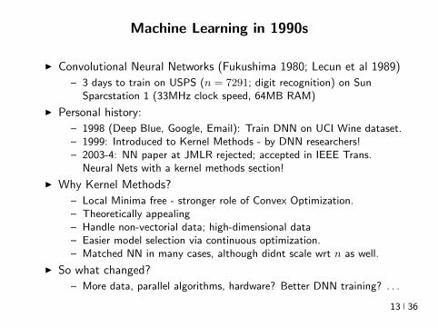
Machine Learning in 1990s
I Convolutional Neural Networks (Fukushima 1980 Lecun et al 1989)
ndash 3 days to train on USPS (n = 7291 digit recognition) on SunSparcstation 1 (33MHz clock speed 64MB RAM)
I Personal history
ndash 1998 (Deep Blue Google Email) Train DNN on UCI Wine datasetndash 1999 Introduced to Kernel Methods - by DNN researchersndash 2003-4 NN paper at JMLR rejected accepted in IEEE Trans
Neural Nets with a kernel methods section
I Why Kernel Methods
ndash Local Minima free - stronger role of Convex Optimizationndash Theoretically appealingndash Handle non-vectorial data high-dimensional datandash Easier model selection via continuous optimizationndash Matched NN in many cases although didnt scale wrt n as well
I So what changed
ndash More data parallel algorithms hardware Better DNN training
13 36
Kernel Methods vs Neural Networks (Pre-Google)
14 36
Kernel Methods vs Neural Networks
Geoff Hinton facts meme maintained athttpyannlecuncomexfun
I All kernels that ever dared approaching Geoff Hinton woke upconvolved
I The only kernel Geoff Hinton has ever used is a kernel of truth
I If you defy Geoff Hinton he will maximize your entropy in no timeYour free energy will be gone even before you reach equilibrium
Are there synergies between these fields towards design of even better(faster and more accurate) algorithms
15 36
Kernel Methods vs Neural Networks
Geoff Hinton facts meme maintained athttpyannlecuncomexfun
I All kernels that ever dared approaching Geoff Hinton woke upconvolved
I The only kernel Geoff Hinton has ever used is a kernel of truth
I If you defy Geoff Hinton he will maximize your entropy in no timeYour free energy will be gone even before you reach equilibrium
Are there synergies between these fields towards design of even better(faster and more accurate) algorithms
15 36
Kernel Methods vs Neural Networks
Geoff Hinton facts meme maintained athttpyannlecuncomexfun
I All kernels that ever dared approaching Geoff Hinton woke upconvolved
I The only kernel Geoff Hinton has ever used is a kernel of truth
I If you defy Geoff Hinton he will maximize your entropy in no timeYour free energy will be gone even before you reach equilibrium
Are there synergies between these fields towards design of even better(faster and more accurate) algorithms
15 36
Linear Hypotheses
I f(x) = wTxw isin Rn Assume Y sub R setting
arg minwisinRd
lsumi=1
(yi minuswTxi)2 + λw22
w = (XTX + λId)minus1 (XTy
)X =
xTi
isin Rltimesn
I ntimes n linear system =rArr O(ln2 + n3) training time assuming nostructure (eg sparsity)
I O(n) prediction time
I High Approximation error
16 36
Polynomials The expensive way
I Homogeneous degree-d polynomial
f(x) = wTΨnd(x) w isin Rs s =
(d+ nminus 1
d
)
Ψnd(x) =
radic(dα
)xα
isin Rs
α = (α1 αn)sumi
αi = d
(d
α
)=
d
α1 αn
xα = xα11 xα2
2 xαnn
I Construct Z isin Rntimess with rows Ψnd(xi) and solve in O(s3) () time
w = (ZTZ + λId)minus1 (ZTy) (1)
I Note n = 100 d = 4 =rArr s gt 4M
17 36
Polynomials
I Consider the subspace of Rs spanned by the data
S = span (Ψ(x1) Ψ(xl)) = v isin Rs v =
lsumi=1
αiΨ(xi)
I So Rs = S + Sperp Hence for any vector w isin Rs
w = wS + wSperp
I The search of a minimizer can be reduced to S because
lsumi=1
V (wTΨ(xi)) + λw22 gelsumi=1
V (wTSΨ(xi)) + λwS22 + wperpS 22
gelsumi=1
V (wTSΨ(xi)) + λwS22 (2)
I Argument holds for any loss (convex or non-convex additive or not)but needs orthogonality (l2 regularizer) [Representer Theorem]
18 36
Polynomials
I Consider the subspace of Rs spanned by the data
S = span (Ψ(x1) Ψ(xl)) = v isin Rs v =
lsumi=1
αiΨ(xi)
I So Rs = S + Sperp Hence for any vector w isin Rs
w = wS + wSperp
I The search of a minimizer can be reduced to S because
lsumi=1
V (wTΨ(xi)) + λw22 gelsumi=1
V (wTSΨ(xi)) + λwS22 + wperpS 22
gelsumi=1
V (wTSΨ(xi)) + λwS22 (2)
I Argument holds for any loss (convex or non-convex additive or not)but needs orthogonality (l2 regularizer) [Representer Theorem]
18 36
Polynomials
I Consider the subspace of Rs spanned by the data
S = span (Ψ(x1) Ψ(xl)) = v isin Rs v =
lsumi=1
αiΨ(xi)
I So Rs = S + Sperp Hence for any vector w isin Rs
w = wS + wSperp
I The search of a minimizer can be reduced to S because
lsumi=1
V (wTΨ(xi)) + λw22 gelsumi=1
V (wTSΨ(xi)) + λwS22 + wperpS 22
gelsumi=1
V (wTSΨ(xi)) + λwS22 (2)
I Argument holds for any loss (convex or non-convex additive or not)but needs orthogonality (l2 regularizer) [Representer Theorem]
18 36
Polynomials
I Consider the subspace of Rs spanned by the data
S = span (Ψ(x1) Ψ(xl)) = v isin Rs v =
lsumi=1
αiΨ(xi)
I So Rs = S + Sperp Hence for any vector w isin Rs
w = wS + wSperp
I The search of a minimizer can be reduced to S because
lsumi=1
V (wTΨ(xi)) + λw22 gelsumi=1
V (wTSΨ(xi)) + λwS22 + wperpS 22
gelsumi=1
V (wTSΨ(xi)) + λwS22 (2)
I Argument holds for any loss (convex or non-convex additive or not)but needs orthogonality (l2 regularizer) [Representer Theorem]
18 36
Polynomials
I Hence w =sumli=1 βiΨ(xi) isin S for β isin Rl and so we can solve
arg minwisinRd
lsumi=1
(yi minuswTΨ(xi))2 + λw22
arg minβisinRl
lsumj=1
(yj minus
lsumi=1
βiΨ(xi)TΨ(xj)
)2
+ λ
lsumij=1
βiβjΨ(xi)TΨ(xj)
arg minβisinRl
lsumj=1
(yj minus (Gβ)j
)2+ λβTGβ
Gij = Ψ(xi)TΨ(xj)
β = (G + λId)minus1
y
I O(l3 + sl2) training time - O(s3) cost eliminatedI Inference time (O(s) or O(ls))
f(x) = wTΨ(x) =
lsumi=1
βiΨ(xi)TΨ(x)
19 36
Polynomials
I Hence w =sumli=1 βiΨ(xi) isin S for β isin Rl and so we can solve
arg minwisinRd
lsumi=1
(yi minuswTΨ(xi))2 + λw22
arg minβisinRl
lsumj=1
(yj minus
lsumi=1
βiΨ(xi)TΨ(xj)
)2
+ λ
lsumij=1
βiβjΨ(xi)TΨ(xj)
arg minβisinRl
lsumj=1
(yj minus (Gβ)j
)2+ λβTGβ
Gij = Ψ(xi)TΨ(xj)
β = (G + λId)minus1
y
I O(l3 + sl2) training time - O(s3) cost eliminatedI Inference time (O(s) or O(ls))
f(x) = wTΨ(x) =
lsumi=1
βiΨ(xi)TΨ(x)
19 36
Polynomials
I Hence w =sumli=1 βiΨ(xi) isin S for β isin Rl and so we can solve
arg minwisinRd
lsumi=1
(yi minuswTΨ(xi))2 + λw22
arg minβisinRl
lsumj=1
(yj minus
lsumi=1
βiΨ(xi)TΨ(xj)
)2
+ λ
lsumij=1
βiβjΨ(xi)TΨ(xj)
arg minβisinRl
lsumj=1
(yj minus (Gβ)j
)2+ λβTGβ
Gij = Ψ(xi)TΨ(xj)
β = (G + λId)minus1
y
I O(l3 + sl2) training time - O(s3) cost eliminatedI Inference time (O(s) or O(ls))
f(x) = wTΨ(x) =
lsumi=1
βiΨ(xi)TΨ(x)
19 36
Polynomials
I Multinomial Theorem
(z1 + z2 + + zn)d =sum
α|α|=d
(d
α
)zα
I Implicit computation of inner products
Ψ(x)TΨ(xprime) =
ssumi=1
(d
α
)xαxprime
α=
ssumi=1
(d
α
)xα11 xαnn x
primeα11 x
primeαnn
=
ssumi=1
(d
α
)(x1x
prime1)α1(x2x
prime2)α2 (xnx
primen)αn
= (x1xprime1 + xnx
primen)d
= (xTxprime)d
I O(l3 + l2n) training and O(ln) predicting speedI Complexity coming from s has been completely eliminated ()
[Kernel Trick]
20 36
Polynomials
I Multinomial Theorem
(z1 + z2 + + zn)d =sum
α|α|=d
(d
α
)zα
I Implicit computation of inner products
Ψ(x)TΨ(xprime) =
ssumi=1
(d
α
)xαxprime
α=
ssumi=1
(d
α
)xα11 xαnn x
primeα11 x
primeαnn
=
ssumi=1
(d
α
)(x1x
prime1)α1(x2x
prime2)α2 (xnx
primen)αn
= (x1xprime1 + xnx
primen)d
= (xTxprime)d
I O(l3 + l2n) training and O(ln) predicting speedI Complexity coming from s has been completely eliminated ()
[Kernel Trick]
20 36
Polynomials
I Multinomial Theorem
(z1 + z2 + + zn)d =sum
α|α|=d
(d
α
)zα
I Implicit computation of inner products
Ψ(x)TΨ(xprime) =
ssumi=1
(d
α
)xαxprime
α=
ssumi=1
(d
α
)xα11 xαnn x
primeα11 x
primeαnn
=
ssumi=1
(d
α
)(x1x
prime1)α1(x2x
prime2)α2 (xnx
primen)αn
= (x1xprime1 + xnx
primen)d
= (xTxprime)d
I O(l3 + l2n) training and O(ln) predicting speedI Complexity coming from s has been completely eliminated ()
[Kernel Trick]
20 36
Polynomials
I Multinomial Theorem
(z1 + z2 + + zn)d =sum
α|α|=d
(d
α
)zα
I Implicit computation of inner products
Ψ(x)TΨ(xprime) =
ssumi=1
(d
α
)xαxprime
α=
ssumi=1
(d
α
)xα11 xαnn x
primeα11 x
primeαnn
=
ssumi=1
(d
α
)(x1x
prime1)α1(x2x
prime2)α2 (xnx
primen)αn
= (x1xprime1 + xnx
primen)d
= (xTxprime)d
I O(l3 + l2n) training and O(ln) predicting speedI Complexity coming from s has been completely eliminated ()
[Kernel Trick]
20 36
Polynomials
I Multinomial Theorem
(z1 + z2 + + zn)d =sum
α|α|=d
(d
α
)zα
I Implicit computation of inner products
Ψ(x)TΨ(xprime) =
ssumi=1
(d
α
)xαxprime
α=
ssumi=1
(d
α
)xα11 xαnn x
primeα11 x
primeαnn
=
ssumi=1
(d
α
)(x1x
prime1)α1(x2x
prime2)α2 (xnx
primen)αn
= (x1xprime1 + xnx
primen)d
= (xTxprime)d
I O(l3 + l2n) training and O(ln) predicting speedI Complexity coming from s has been completely eliminated ()
[Kernel Trick]
20 36
Polynomials Algorithm
I Algorithm
ndash Start with k X times X 7rarr R k(xxprime) = (xTxprime + 1)d
ndash Construct Gram matrix Gij = k(xixj) on the training samplesndash Solve β = (G + λId)minus1 yndash Return f(x) =
sumli=1 βik(xix)
I f is the optimal degree-d polynomial solving the learning problemin complexity independent of d
I What other forms of k correspond to linear learning inhigh-dimensional nonlinear embeddings of the data
21 36
Polynomials Algorithm
I Algorithm
ndash Start with k X times X 7rarr R k(xxprime) = (xTxprime + 1)d
ndash Construct Gram matrix Gij = k(xixj) on the training samplesndash Solve β = (G + λId)minus1 yndash Return f(x) =
sumli=1 βik(xix)
I f is the optimal degree-d polynomial solving the learning problemin complexity independent of d
I What other forms of k correspond to linear learning inhigh-dimensional nonlinear embeddings of the data
21 36
Symmetric positive semi-definite functions
I Definition A function k X times X 7rarr R is psd if for any finitecollection of points x1 xl the l times l Gram matrix
Gij = k(xixj)
is positive semi-definite ie for any vector β isin Rl
βTGβ =sumij
βiβjk(xixj) ge 0
I Theorem[Mercer] If k is symmetric psd X is compact subset ofRn then it admits an eigenfunction decomposition
k(xxprime) =
Nsumi=1
λiφj(x)φj(xprime) = 〈Ψ(x)Ψ(xprime)〉l2
Ψ(x) = [ radicλjφ(x) ]T (3)
I Feature map associated with a kernel is not uniqueI Functional generalization of positive semi-definite matrices
22 36
Symmetric positive semi-definite functions
I Definition A function k X times X 7rarr R is psd if for any finitecollection of points x1 xl the l times l Gram matrix
Gij = k(xixj)
is positive semi-definite ie for any vector β isin Rl
βTGβ =sumij
βiβjk(xixj) ge 0
I Theorem[Mercer] If k is symmetric psd X is compact subset ofRn then it admits an eigenfunction decomposition
k(xxprime) =
Nsumi=1
λiφj(x)φj(xprime) = 〈Ψ(x)Ψ(xprime)〉l2
Ψ(x) = [ radicλjφ(x) ]T (3)
I Feature map associated with a kernel is not uniqueI Functional generalization of positive semi-definite matrices
22 36
Kernels
I Lineark(xxprime) = xTxprime
I Polynomialk(xxprime) = (xTxprime + 1)d
I Gaussian s =infin Universal
k(xxprime) = eminusxminusxprime2
2σ2
I Conic combinations
k(xxprime) = α1k1(xxprime) + α2k2(xxprime)
I Elementwise products
k(xxprime) = k1(xxprime)k2(xxprime)
I Kernels on discrete sets strings graphs sequences shapes
23 36
Kernels
I Lineark(xxprime) = xTxprime
I Polynomialk(xxprime) = (xTxprime + 1)d
I Gaussian s =infin Universal
k(xxprime) = eminusxminusxprime2
2σ2
I Conic combinations
k(xxprime) = α1k1(xxprime) + α2k2(xxprime)
I Elementwise products
k(xxprime) = k1(xxprime)k2(xxprime)
I Kernels on discrete sets strings graphs sequences shapes
23 36
Kernels
I Lineark(xxprime) = xTxprime
I Polynomialk(xxprime) = (xTxprime + 1)d
I Gaussian s =infin Universal
k(xxprime) = eminusxminusxprime2
2σ2
I Conic combinations
k(xxprime) = α1k1(xxprime) + α2k2(xxprime)
I Elementwise products
k(xxprime) = k1(xxprime)k2(xxprime)
I Kernels on discrete sets strings graphs sequences shapes
23 36
Gaussian Kernel is Positive Definite
I Exponential
eβxTxprime = 1 + βxTxprime +
β2
2(xTy)2 +
β3
3(xTy)3 +
I For any function f Rn 7rarr R psd function k the following kernelis psd
kprime(xxprime) = f(x) (k(xxprime)) f(xprime)
Proofsumij
βiβjkprime(xixj) =
sumij
βiβjf(xi)k(xixj)f(xj) =sumij
βprimeiβprimejk(xixj) ge 0
I Gaussian Kernel
k(xxprime) = eminusxminusxprime22
2σ2
= eminusx222σ2
(e
2xT xprime2σ2
)eminusxprime222σ2 (4)
24 36
Gaussian Kernel is Positive Definite
I Exponential
eβxTxprime = 1 + βxTxprime +
β2
2(xTy)2 +
β3
3(xTy)3 +
I For any function f Rn 7rarr R psd function k the following kernelis psd
kprime(xxprime) = f(x) (k(xxprime)) f(xprime)
Proofsumij
βiβjkprime(xixj) =
sumij
βiβjf(xi)k(xixj)f(xj) =sumij
βprimeiβprimejk(xixj) ge 0
I Gaussian Kernel
k(xxprime) = eminusxminusxprime22
2σ2
= eminusx222σ2
(e
2xT xprime2σ2
)eminusxprime222σ2 (4)
24 36
Gaussian Kernel is Positive Definite
I Exponential
eβxTxprime = 1 + βxTxprime +
β2
2(xTy)2 +
β3
3(xTy)3 +
I For any function f Rn 7rarr R psd function k the following kernelis psd
kprime(xxprime) = f(x) (k(xxprime)) f(xprime)
Proofsumij
βiβjkprime(xixj) =
sumij
βiβjf(xi)k(xixj)f(xj) =sumij
βprimeiβprimejk(xixj) ge 0
I Gaussian Kernel
k(xxprime) = eminusxminusxprime22
2σ2
= eminusx222σ2
(e
2xT xprime2σ2
)eminusxprime222σ2 (4)
24 36
The Mathematical Naturalness of Kernel Methods
I Data X isin Rd Models isin H X 7rarr R
I Geometry in H inner product 〈middot middot〉H norm middot H (Hilbert Spaces)I Theorem All nice Hilbert spaces are generated by a symmetric
positive definite function (the kernel) k(xxprime) on X times XI if f g isin H close ie f minus gH small then f(x) g(x) close forallx isin X I Reproducing Kernel Hilbert Spaces (RKHSs) Hilbert space H
that admit a reproducing kernel ie a function k(xxprime) satisfying
(i) forallx isin X k(middotx) isin H(ii) 〈f k(middotx)〉H = f(x)
I Reproducing kernels are symmetric psdsumij
βiβjk(xixj) = 〈sumi
βik(middotxi)sumi
βik(middotxi)〉H
= sumi
βik(middotxi)2H ge 0 (5)
I (Moore-Aronsjan 1950) Symmetric psd functions arereproducing kernels for some (unique) RKHS Hk
25 36
The Mathematical Naturalness of Kernel Methods
I Data X isin Rd Models isin H X 7rarr RI Geometry in H inner product 〈middot middot〉H norm middot H (Hilbert Spaces)
I Theorem All nice Hilbert spaces are generated by a symmetricpositive definite function (the kernel) k(xxprime) on X times X
I if f g isin H close ie f minus gH small then f(x) g(x) close forallx isin X I Reproducing Kernel Hilbert Spaces (RKHSs) Hilbert space H
that admit a reproducing kernel ie a function k(xxprime) satisfying
(i) forallx isin X k(middotx) isin H(ii) 〈f k(middotx)〉H = f(x)
I Reproducing kernels are symmetric psdsumij
βiβjk(xixj) = 〈sumi
βik(middotxi)sumi
βik(middotxi)〉H
= sumi
βik(middotxi)2H ge 0 (5)
I (Moore-Aronsjan 1950) Symmetric psd functions arereproducing kernels for some (unique) RKHS Hk
25 36
The Mathematical Naturalness of Kernel Methods
I Data X isin Rd Models isin H X 7rarr RI Geometry in H inner product 〈middot middot〉H norm middot H (Hilbert Spaces)I Theorem All nice Hilbert spaces are generated by a symmetric
positive definite function (the kernel) k(xxprime) on X times XI if f g isin H close ie f minus gH small then f(x) g(x) close forallx isin X
I Reproducing Kernel Hilbert Spaces (RKHSs) Hilbert space Hthat admit a reproducing kernel ie a function k(xxprime) satisfying
(i) forallx isin X k(middotx) isin H(ii) 〈f k(middotx)〉H = f(x)
I Reproducing kernels are symmetric psdsumij
βiβjk(xixj) = 〈sumi
βik(middotxi)sumi
βik(middotxi)〉H
= sumi
βik(middotxi)2H ge 0 (5)
I (Moore-Aronsjan 1950) Symmetric psd functions arereproducing kernels for some (unique) RKHS Hk
25 36
The Mathematical Naturalness of Kernel Methods
I Data X isin Rd Models isin H X 7rarr RI Geometry in H inner product 〈middot middot〉H norm middot H (Hilbert Spaces)I Theorem All nice Hilbert spaces are generated by a symmetric
positive definite function (the kernel) k(xxprime) on X times XI if f g isin H close ie f minus gH small then f(x) g(x) close forallx isin X I Reproducing Kernel Hilbert Spaces (RKHSs) Hilbert space H
that admit a reproducing kernel ie a function k(xxprime) satisfying
(i) forallx isin X k(middotx) isin H(ii) 〈f k(middotx)〉H = f(x)
I Reproducing kernels are symmetric psdsumij
βiβjk(xixj) = 〈sumi
βik(middotxi)sumi
βik(middotxi)〉H
= sumi
βik(middotxi)2H ge 0 (5)
I (Moore-Aronsjan 1950) Symmetric psd functions arereproducing kernels for some (unique) RKHS Hk
25 36
The Mathematical Naturalness of Kernel Methods
I Data X isin Rd Models isin H X 7rarr RI Geometry in H inner product 〈middot middot〉H norm middot H (Hilbert Spaces)I Theorem All nice Hilbert spaces are generated by a symmetric
positive definite function (the kernel) k(xxprime) on X times XI if f g isin H close ie f minus gH small then f(x) g(x) close forallx isin X I Reproducing Kernel Hilbert Spaces (RKHSs) Hilbert space H
that admit a reproducing kernel ie a function k(xxprime) satisfying
(i) forallx isin X k(middotx) isin H(ii) 〈f k(middotx)〉H = f(x)
I Reproducing kernels are symmetric psdsumij
βiβjk(xixj) = 〈sumi
βik(middotxi)sumi
βik(middotxi)〉H
= sumi
βik(middotxi)2H ge 0 (5)
I (Moore-Aronsjan 1950) Symmetric psd functions arereproducing kernels for some (unique) RKHS Hk 25 36
Kernel Methods Summary
I Symm pos def function k(x z) on input domain X sub Rd
I k hArr rich Reproducing Kernel Hilbert Space (RKHS) Hk ofreal-valued functions with inner product 〈middot middot〉k and norm middot k
I Regularized Risk Minimization hArr Linear models in an implicithigh-dimensional (often infinite-dimensional) feature space
f = arg minfisinHk
1
n
nsumi=1
V (yi f(xi)) + λf2Hk xi isin Rd
I Representer Theorem f(x) =sumni=1 αik(xxi)
26 36
Shallow and Deep Function Spaces
I What does it mean to understand a function space
ndash Linear f(x) = wTxw isin Rd
ndash Polynomial f(x) = wT Ψ(x)w isin Rs
ndash RKHS balls f isin Hk fk lt γ [like vM le 1]
I Shallow nets f(x) = wTσ(Wx) (w isin RdW isin Rs)ndash For srarrinfin W sim p σ(u) = eminusiu approximates Gaussian kernel
methodsndash Theorem [Bochner 1937] One-to-one correspondence between k
and a density p such that
k(x z) = ψ(xminus z) =
intRdeminusi(xminusz)Twp(w)dw asymp 1
s
ssumj=1
eminusi(xminusz)Twj
Gaussian kernel k(x z) = eminusxminusz22
2σ2 lArrrArr p = N (0 σminus2Id)ndash Similar integral approx relates ReLU to the arc-cosine kernelndash Optimization versus Randomization
27 36
Shallow and Deep Function Spaces
I What does it mean to understand a function space
ndash Linear f(x) = wTxw isin Rd
ndash Polynomial f(x) = wT Ψ(x)w isin Rs
ndash RKHS balls f isin Hk fk lt γ [like vM le 1]
I Shallow nets f(x) = wTσ(Wx) (w isin RdW isin Rs)ndash For srarrinfin W sim p σ(u) = eminusiu approximates Gaussian kernel
methodsndash Theorem [Bochner 1937] One-to-one correspondence between k
and a density p such that
k(x z) = ψ(xminus z) =
intRdeminusi(xminusz)Twp(w)dw asymp 1
s
ssumj=1
eminusi(xminusz)Twj
Gaussian kernel k(x z) = eminusxminusz22
2σ2 lArrrArr p = N (0 σminus2Id)ndash Similar integral approx relates ReLU to the arc-cosine kernelndash Optimization versus Randomization
27 36
Shallow and Deep Function Spaces
I What does it mean to understand a function space
ndash Linear f(x) = wTxw isin Rd
ndash Polynomial f(x) = wT Ψ(x)w isin Rs
ndash RKHS balls f isin Hk fk lt γ [like vM le 1]
I Shallow nets f(x) = wTσ(Wx) (w isin RdW isin Rs)ndash For srarrinfin W sim p σ(u) = eminusiu approximates Gaussian kernel
methodsndash Theorem [Bochner 1937] One-to-one correspondence between k
and a density p such that
k(x z) = ψ(xminus z) =
intRdeminusi(xminusz)Twp(w)dw asymp 1
s
ssumj=1
eminusi(xminusz)Twj
Gaussian kernel k(x z) = eminusxminusz22
2σ2 lArrrArr p = N (0 σminus2Id)ndash Similar integral approx relates ReLU to the arc-cosine kernelndash Optimization versus Randomization
27 36
Shallow and Deep Function Spaces
I What does it mean to understand a function space
ndash Linear f(x) = wTxw isin Rd
ndash Polynomial f(x) = wT Ψ(x)w isin Rs
ndash RKHS balls f isin Hk fk lt γ [like vM le 1]
I Shallow nets f(x) = wTσ(Wx) (w isin RdW isin Rs)
ndash For srarrinfin W sim p σ(u) = eminusiu approximates Gaussian kernelmethods
ndash Theorem [Bochner 1937] One-to-one correspondence between kand a density p such that
k(x z) = ψ(xminus z) =
intRdeminusi(xminusz)Twp(w)dw asymp 1
s
ssumj=1
eminusi(xminusz)Twj
Gaussian kernel k(x z) = eminusxminusz22
2σ2 lArrrArr p = N (0 σminus2Id)ndash Similar integral approx relates ReLU to the arc-cosine kernelndash Optimization versus Randomization
27 36
Shallow and Deep Function Spaces
I What does it mean to understand a function space
ndash Linear f(x) = wTxw isin Rd
ndash Polynomial f(x) = wT Ψ(x)w isin Rs
ndash RKHS balls f isin Hk fk lt γ [like vM le 1]
I Shallow nets f(x) = wTσ(Wx) (w isin RdW isin Rs)ndash For srarrinfin W sim p σ(u) = eminusiu approximates Gaussian kernel
methodsndash Theorem [Bochner 1937] One-to-one correspondence between k
and a density p such that
k(x z) = ψ(xminus z) =
intRdeminusi(xminusz)Twp(w)dw asymp 1
s
ssumj=1
eminusi(xminusz)Twj
Gaussian kernel k(x z) = eminusxminusz22
2σ2 lArrrArr p = N (0 σminus2Id)ndash Similar integral approx relates ReLU to the arc-cosine kernelndash Optimization versus Randomization
27 36
Expressivity of Deep Nets Linear Regions
I The ReLU map f(x) = max(Wx 0)W isin Rwtimesn is piecewise linear
I A piece is a connected region (a convex polytope) of Rd with sharedsparsity pattern in activations
I (Zaslavsky 1975) Number of linear regions formed by an arrangement of
s hyperplanes in d-dimensions in general position issumd
i=0
(si
)I Composition of ReLU maps is also piecewise linear
I (Raghu et al 2017 Pascano et al 2014 Montufar 2014) Number oflinear regions grows as O(wnd) for a composition of d ReLU maps(nrarr brarr brarr b rarr b) each of width w
I (Safran and Shamir 2017)
ndash 1[x le 1] x isin Rd ε-accurate 3-layer network with O(dε) neurons but cannot be approximated with
accuracy higher than O(1d4) using 2-layer networks unless width is exponential in d
28 36
Expressivity of Deep Nets Linear Regions
I The ReLU map f(x) = max(Wx 0)W isin Rwtimesn is piecewise linear
I A piece is a connected region (a convex polytope) of Rd with sharedsparsity pattern in activations
I (Zaslavsky 1975) Number of linear regions formed by an arrangement of
s hyperplanes in d-dimensions in general position issumd
i=0
(si
)I Composition of ReLU maps is also piecewise linear
I (Raghu et al 2017 Pascano et al 2014 Montufar 2014) Number oflinear regions grows as O(wnd) for a composition of d ReLU maps(nrarr brarr brarr b rarr b) each of width w
I (Safran and Shamir 2017)
ndash 1[x le 1] x isin Rd ε-accurate 3-layer network with O(dε) neurons but cannot be approximated with
accuracy higher than O(1d4) using 2-layer networks unless width is exponential in d
28 36
Expressivity of Deep Nets Linear Regions
I The ReLU map f(x) = max(Wx 0)W isin Rwtimesn is piecewise linear
I A piece is a connected region (a convex polytope) of Rd with sharedsparsity pattern in activations
I (Zaslavsky 1975) Number of linear regions formed by an arrangement of
s hyperplanes in d-dimensions in general position issumd
i=0
(si
)
I Composition of ReLU maps is also piecewise linear
I (Raghu et al 2017 Pascano et al 2014 Montufar 2014) Number oflinear regions grows as O(wnd) for a composition of d ReLU maps(nrarr brarr brarr b rarr b) each of width w
I (Safran and Shamir 2017)
ndash 1[x le 1] x isin Rd ε-accurate 3-layer network with O(dε) neurons but cannot be approximated with
accuracy higher than O(1d4) using 2-layer networks unless width is exponential in d
28 36
Expressivity of Deep Nets Linear Regions
I The ReLU map f(x) = max(Wx 0)W isin Rwtimesn is piecewise linear
I A piece is a connected region (a convex polytope) of Rd with sharedsparsity pattern in activations
I (Zaslavsky 1975) Number of linear regions formed by an arrangement of
s hyperplanes in d-dimensions in general position issumd
i=0
(si
)I Composition of ReLU maps is also piecewise linear
I (Raghu et al 2017 Pascano et al 2014 Montufar 2014) Number oflinear regions grows as O(wnd) for a composition of d ReLU maps(nrarr brarr brarr b rarr b) each of width w
I (Safran and Shamir 2017)
ndash 1[x le 1] x isin Rd ε-accurate 3-layer network with O(dε) neurons but cannot be approximated with
accuracy higher than O(1d4) using 2-layer networks unless width is exponential in d28 36
Expressivity of Deep Nets Trajectory Length
I (Raghu et al 2017) Trajectory Length (ldquogeneralized operator normrdquo)How much is a curve in the input space stretched by a layer in thenetwork
29 36
Expressivity of Deep Nets Trajectory Length
I (Raghu et al 2017) Trajectory Length (ldquogeneralized operator normrdquo)How much is a curve in the input space stretched by a layer in thenetwork
29 36
Expressivity and Generalization
I Expressiveness equiv capacity to fit random noise =rArr susceptibility tooverfitting (VC dimension Rademacher Complexity)
I Zhang et al 2017 Famous CNNs easily fit random labels
ndash Over-parameterized (n=12M psim 60M) but structuredndash Domain-knowledge baked in does not constraint expressiveness
I CNNs tend to generalize even without regularization (explicit and implicit)
I For linear regression SGD returns minimum norm solution
30 36
Expressivity and Generalization
I Expressiveness equiv capacity to fit random noise =rArr susceptibility tooverfitting (VC dimension Rademacher Complexity)
I Zhang et al 2017 Famous CNNs easily fit random labels
ndash Over-parameterized (n=12M psim 60M) but structuredndash Domain-knowledge baked in does not constraint expressiveness
I CNNs tend to generalize even without regularization (explicit and implicit)
I For linear regression SGD returns minimum norm solution
30 36
Expressivity and Generalization
I Expressiveness equiv capacity to fit random noise =rArr susceptibility tooverfitting (VC dimension Rademacher Complexity)
I Zhang et al 2017 Famous CNNs easily fit random labels
ndash Over-parameterized (n=12M psim 60M) but structuredndash Domain-knowledge baked in does not constraint expressiveness
I CNNs tend to generalize even without regularization (explicit and implicit)
I For linear regression SGD returns minimum norm solution
30 36
Optimization Landscape Symmetry and Saddle Points
I Folklore lots of equivalent good local minI Classification of critical points based on Hessian spectrumI Permutation and Scaling symmetries
I Thm [Lee et al 2016 Anadkumar Ge] For the short-step gradientmethod the basin of attraction of strict saddle points (atleast onenegative eigenvalue) has measure zero
31 36
Optimization Landscape Symmetry and Saddle Points
I Folklore lots of equivalent good local minI Classification of critical points based on Hessian spectrumI Permutation and Scaling symmetries
I Thm [Lee et al 2016 Anadkumar Ge] For the short-step gradientmethod the basin of attraction of strict saddle points (atleast onenegative eigenvalue) has measure zero
31 36
Optimization Landscape Symmetry and Saddle Points
I Folklore lots of equivalent good local minI Classification of critical points based on Hessian spectrumI Permutation and Scaling symmetries
I Thm [Lee et al 2016 Anadkumar Ge] For the short-step gradientmethod the basin of attraction of strict saddle points (atleast onenegative eigenvalue) has measure zero
31 36
Optimization Landscape Sharp Minima and Stability
Keskar et al 2017 On large-batch training for DL Generalization Gap and Sharp Minima
32 36
Deep Learning Computational Graphs TensorFlow
tensorfloworg
I Tensors-in Tensors-out
I Evergrowing list of Tensor-Ops (PythonC++)
f(xw)
[partf
partx
]T v
[partf
partw
]T v
I Automatic Differentiation Reverse mode
partxL
partxi=sumirarrj
partxL
partxj
partxj
partxi
33 36
Computational Graphs and TensorFlow
tensorfloworg
I SGD with minibatches
wk+1 = wk minus ηlsumi=1
partli
partw
∣∣∣wt
I Model Parallelism Assign independent paths tothreads GPUs
I Data Parallelism create Graph replicas on differentmachines
I Mobile TensorFlow
34 36
Computational Graphs and TensorFlow
tensorfloworg
35 36
Computational Graphs and TensorFlow
tensorfloworg
35 36
Computational Graphs and TensorFlow
tensorfloworg
35 36
Challenges and Opportunities
I Lots of fascinating unsolved problems
I Can you win Imagenet with Convex optimization
I Tools from polynomial optimization (global optimization deep-RL)
I Supervised to Semi-supervised to Unsupervised Learning
I Compact efficient real-time models (eliminateover-parametrization) for new form factors
I Exciting emerging world of Robotics Wearable ComputersIntelligent home devices Personal digital assistants
Google Internship Program
36 36
- anm0
- fdrm0
- fdrm5
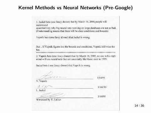
Kernel Methods vs Neural Networks
Geoff Hinton facts meme maintained athttpyannlecuncomexfun
I All kernels that ever dared approaching Geoff Hinton woke upconvolved
I The only kernel Geoff Hinton has ever used is a kernel of truth
I If you defy Geoff Hinton he will maximize your entropy in no timeYour free energy will be gone even before you reach equilibrium
Are there synergies between these fields towards design of even better(faster and more accurate) algorithms
15 36
Linear Hypotheses
I f(x) = wTxw isin Rn Assume Y sub R setting
arg minwisinRd
lsumi=1
(yi minuswTxi)2 + λw22
w = (XTX + λId)minus1 (XTy
)X =
xTi
isin Rltimesn
I ntimes n linear system =rArr O(ln2 + n3) training time assuming nostructure (eg sparsity)
I O(n) prediction time
I High Approximation error
16 36
Polynomials The expensive way
I Homogeneous degree-d polynomial
f(x) = wTΨnd(x) w isin Rs s =
(d+ nminus 1
d
)
Ψnd(x) =
radic(dα
)xα
isin Rs
α = (α1 αn)sumi
αi = d
(d
α
)=
d
α1 αn
xα = xα11 xα2
2 xαnn
I Construct Z isin Rntimess with rows Ψnd(xi) and solve in O(s3) () time
w = (ZTZ + λId)minus1 (ZTy) (1)
I Note n = 100 d = 4 =rArr s gt 4M
17 36
Polynomials
I Consider the subspace of Rs spanned by the data
S = span (Ψ(x1) Ψ(xl)) = v isin Rs v =
lsumi=1
αiΨ(xi)
I So Rs = S + Sperp Hence for any vector w isin Rs
w = wS + wSperp
I The search of a minimizer can be reduced to S because
lsumi=1
V (wTΨ(xi)) + λw22 gelsumi=1
V (wTSΨ(xi)) + λwS22 + wperpS 22
gelsumi=1
V (wTSΨ(xi)) + λwS22 (2)
I Argument holds for any loss (convex or non-convex additive or not)but needs orthogonality (l2 regularizer) [Representer Theorem]
18 36
Polynomials
I Consider the subspace of Rs spanned by the data
S = span (Ψ(x1) Ψ(xl)) = v isin Rs v =
lsumi=1
αiΨ(xi)
I So Rs = S + Sperp Hence for any vector w isin Rs
w = wS + wSperp
I The search of a minimizer can be reduced to S because
lsumi=1
V (wTΨ(xi)) + λw22 gelsumi=1
V (wTSΨ(xi)) + λwS22 + wperpS 22
gelsumi=1
V (wTSΨ(xi)) + λwS22 (2)
I Argument holds for any loss (convex or non-convex additive or not)but needs orthogonality (l2 regularizer) [Representer Theorem]
18 36
Polynomials
I Consider the subspace of Rs spanned by the data
S = span (Ψ(x1) Ψ(xl)) = v isin Rs v =
lsumi=1
αiΨ(xi)
I So Rs = S + Sperp Hence for any vector w isin Rs
w = wS + wSperp
I The search of a minimizer can be reduced to S because
lsumi=1
V (wTΨ(xi)) + λw22 gelsumi=1
V (wTSΨ(xi)) + λwS22 + wperpS 22
gelsumi=1
V (wTSΨ(xi)) + λwS22 (2)
I Argument holds for any loss (convex or non-convex additive or not)but needs orthogonality (l2 regularizer) [Representer Theorem]
18 36
Polynomials
I Consider the subspace of Rs spanned by the data
S = span (Ψ(x1) Ψ(xl)) = v isin Rs v =
lsumi=1
αiΨ(xi)
I So Rs = S + Sperp Hence for any vector w isin Rs
w = wS + wSperp
I The search of a minimizer can be reduced to S because
lsumi=1
V (wTΨ(xi)) + λw22 gelsumi=1
V (wTSΨ(xi)) + λwS22 + wperpS 22
gelsumi=1
V (wTSΨ(xi)) + λwS22 (2)
I Argument holds for any loss (convex or non-convex additive or not)but needs orthogonality (l2 regularizer) [Representer Theorem]
18 36
Polynomials
I Hence w =sumli=1 βiΨ(xi) isin S for β isin Rl and so we can solve
arg minwisinRd
lsumi=1
(yi minuswTΨ(xi))2 + λw22
arg minβisinRl
lsumj=1
(yj minus
lsumi=1
βiΨ(xi)TΨ(xj)
)2
+ λ
lsumij=1
βiβjΨ(xi)TΨ(xj)
arg minβisinRl
lsumj=1
(yj minus (Gβ)j
)2+ λβTGβ
Gij = Ψ(xi)TΨ(xj)
β = (G + λId)minus1
y
I O(l3 + sl2) training time - O(s3) cost eliminatedI Inference time (O(s) or O(ls))
f(x) = wTΨ(x) =
lsumi=1
βiΨ(xi)TΨ(x)
19 36
Polynomials
I Hence w =sumli=1 βiΨ(xi) isin S for β isin Rl and so we can solve
arg minwisinRd
lsumi=1
(yi minuswTΨ(xi))2 + λw22
arg minβisinRl
lsumj=1
(yj minus
lsumi=1
βiΨ(xi)TΨ(xj)
)2
+ λ
lsumij=1
βiβjΨ(xi)TΨ(xj)
arg minβisinRl
lsumj=1
(yj minus (Gβ)j
)2+ λβTGβ
Gij = Ψ(xi)TΨ(xj)
β = (G + λId)minus1
y
I O(l3 + sl2) training time - O(s3) cost eliminatedI Inference time (O(s) or O(ls))
f(x) = wTΨ(x) =
lsumi=1
βiΨ(xi)TΨ(x)
19 36
Polynomials
I Hence w =sumli=1 βiΨ(xi) isin S for β isin Rl and so we can solve
arg minwisinRd
lsumi=1
(yi minuswTΨ(xi))2 + λw22
arg minβisinRl
lsumj=1
(yj minus
lsumi=1
βiΨ(xi)TΨ(xj)
)2
+ λ
lsumij=1
βiβjΨ(xi)TΨ(xj)
arg minβisinRl
lsumj=1
(yj minus (Gβ)j
)2+ λβTGβ
Gij = Ψ(xi)TΨ(xj)
β = (G + λId)minus1
y
I O(l3 + sl2) training time - O(s3) cost eliminatedI Inference time (O(s) or O(ls))
f(x) = wTΨ(x) =
lsumi=1
βiΨ(xi)TΨ(x)
19 36
Polynomials
I Multinomial Theorem
(z1 + z2 + + zn)d =sum
α|α|=d
(d
α
)zα
I Implicit computation of inner products
Ψ(x)TΨ(xprime) =
ssumi=1
(d
α
)xαxprime
α=
ssumi=1
(d
α
)xα11 xαnn x
primeα11 x
primeαnn
=
ssumi=1
(d
α
)(x1x
prime1)α1(x2x
prime2)α2 (xnx
primen)αn
= (x1xprime1 + xnx
primen)d
= (xTxprime)d
I O(l3 + l2n) training and O(ln) predicting speedI Complexity coming from s has been completely eliminated ()
[Kernel Trick]
20 36
Polynomials
I Multinomial Theorem
(z1 + z2 + + zn)d =sum
α|α|=d
(d
α
)zα
I Implicit computation of inner products
Ψ(x)TΨ(xprime) =
ssumi=1
(d
α
)xαxprime
α=
ssumi=1
(d
α
)xα11 xαnn x
primeα11 x
primeαnn
=
ssumi=1
(d
α
)(x1x
prime1)α1(x2x
prime2)α2 (xnx
primen)αn
= (x1xprime1 + xnx
primen)d
= (xTxprime)d
I O(l3 + l2n) training and O(ln) predicting speedI Complexity coming from s has been completely eliminated ()
[Kernel Trick]
20 36
Polynomials
I Multinomial Theorem
(z1 + z2 + + zn)d =sum
α|α|=d
(d
α
)zα
I Implicit computation of inner products
Ψ(x)TΨ(xprime) =
ssumi=1
(d
α
)xαxprime
α=
ssumi=1
(d
α
)xα11 xαnn x
primeα11 x
primeαnn
=
ssumi=1
(d
α
)(x1x
prime1)α1(x2x
prime2)α2 (xnx
primen)αn
= (x1xprime1 + xnx
primen)d
= (xTxprime)d
I O(l3 + l2n) training and O(ln) predicting speedI Complexity coming from s has been completely eliminated ()
[Kernel Trick]
20 36
Polynomials
I Multinomial Theorem
(z1 + z2 + + zn)d =sum
α|α|=d
(d
α
)zα
I Implicit computation of inner products
Ψ(x)TΨ(xprime) =
ssumi=1
(d
α
)xαxprime
α=
ssumi=1
(d
α
)xα11 xαnn x
primeα11 x
primeαnn
=
ssumi=1
(d
α
)(x1x
prime1)α1(x2x
prime2)α2 (xnx
primen)αn
= (x1xprime1 + xnx
primen)d
= (xTxprime)d
I O(l3 + l2n) training and O(ln) predicting speedI Complexity coming from s has been completely eliminated ()
[Kernel Trick]
20 36
Polynomials
I Multinomial Theorem
(z1 + z2 + + zn)d =sum
α|α|=d
(d
α
)zα
I Implicit computation of inner products
Ψ(x)TΨ(xprime) =
ssumi=1
(d
α
)xαxprime
α=
ssumi=1
(d
α
)xα11 xαnn x
primeα11 x
primeαnn
=
ssumi=1
(d
α
)(x1x
prime1)α1(x2x
prime2)α2 (xnx
primen)αn
= (x1xprime1 + xnx
primen)d
= (xTxprime)d
I O(l3 + l2n) training and O(ln) predicting speedI Complexity coming from s has been completely eliminated ()
[Kernel Trick]
20 36
Polynomials Algorithm
I Algorithm
ndash Start with k X times X 7rarr R k(xxprime) = (xTxprime + 1)d
ndash Construct Gram matrix Gij = k(xixj) on the training samplesndash Solve β = (G + λId)minus1 yndash Return f(x) =
sumli=1 βik(xix)
I f is the optimal degree-d polynomial solving the learning problemin complexity independent of d
I What other forms of k correspond to linear learning inhigh-dimensional nonlinear embeddings of the data
21 36
Polynomials Algorithm
I Algorithm
ndash Start with k X times X 7rarr R k(xxprime) = (xTxprime + 1)d
ndash Construct Gram matrix Gij = k(xixj) on the training samplesndash Solve β = (G + λId)minus1 yndash Return f(x) =
sumli=1 βik(xix)
I f is the optimal degree-d polynomial solving the learning problemin complexity independent of d
I What other forms of k correspond to linear learning inhigh-dimensional nonlinear embeddings of the data
21 36
Symmetric positive semi-definite functions
I Definition A function k X times X 7rarr R is psd if for any finitecollection of points x1 xl the l times l Gram matrix
Gij = k(xixj)
is positive semi-definite ie for any vector β isin Rl
βTGβ =sumij
βiβjk(xixj) ge 0
I Theorem[Mercer] If k is symmetric psd X is compact subset ofRn then it admits an eigenfunction decomposition
k(xxprime) =
Nsumi=1
λiφj(x)φj(xprime) = 〈Ψ(x)Ψ(xprime)〉l2
Ψ(x) = [ radicλjφ(x) ]T (3)
I Feature map associated with a kernel is not uniqueI Functional generalization of positive semi-definite matrices
22 36
Symmetric positive semi-definite functions
I Definition A function k X times X 7rarr R is psd if for any finitecollection of points x1 xl the l times l Gram matrix
Gij = k(xixj)
is positive semi-definite ie for any vector β isin Rl
βTGβ =sumij
βiβjk(xixj) ge 0
I Theorem[Mercer] If k is symmetric psd X is compact subset ofRn then it admits an eigenfunction decomposition
k(xxprime) =
Nsumi=1
λiφj(x)φj(xprime) = 〈Ψ(x)Ψ(xprime)〉l2
Ψ(x) = [ radicλjφ(x) ]T (3)
I Feature map associated with a kernel is not uniqueI Functional generalization of positive semi-definite matrices
22 36
Kernels
I Lineark(xxprime) = xTxprime
I Polynomialk(xxprime) = (xTxprime + 1)d
I Gaussian s =infin Universal
k(xxprime) = eminusxminusxprime2
2σ2
I Conic combinations
k(xxprime) = α1k1(xxprime) + α2k2(xxprime)
I Elementwise products
k(xxprime) = k1(xxprime)k2(xxprime)
I Kernels on discrete sets strings graphs sequences shapes
23 36
Kernels
I Lineark(xxprime) = xTxprime
I Polynomialk(xxprime) = (xTxprime + 1)d
I Gaussian s =infin Universal
k(xxprime) = eminusxminusxprime2
2σ2
I Conic combinations
k(xxprime) = α1k1(xxprime) + α2k2(xxprime)
I Elementwise products
k(xxprime) = k1(xxprime)k2(xxprime)
I Kernels on discrete sets strings graphs sequences shapes
23 36
Kernels
I Lineark(xxprime) = xTxprime
I Polynomialk(xxprime) = (xTxprime + 1)d
I Gaussian s =infin Universal
k(xxprime) = eminusxminusxprime2
2σ2
I Conic combinations
k(xxprime) = α1k1(xxprime) + α2k2(xxprime)
I Elementwise products
k(xxprime) = k1(xxprime)k2(xxprime)
I Kernels on discrete sets strings graphs sequences shapes
23 36
Gaussian Kernel is Positive Definite
I Exponential
eβxTxprime = 1 + βxTxprime +
β2
2(xTy)2 +
β3
3(xTy)3 +
I For any function f Rn 7rarr R psd function k the following kernelis psd
kprime(xxprime) = f(x) (k(xxprime)) f(xprime)
Proofsumij
βiβjkprime(xixj) =
sumij
βiβjf(xi)k(xixj)f(xj) =sumij
βprimeiβprimejk(xixj) ge 0
I Gaussian Kernel
k(xxprime) = eminusxminusxprime22
2σ2
= eminusx222σ2
(e
2xT xprime2σ2
)eminusxprime222σ2 (4)
24 36
Gaussian Kernel is Positive Definite
I Exponential
eβxTxprime = 1 + βxTxprime +
β2
2(xTy)2 +
β3
3(xTy)3 +
I For any function f Rn 7rarr R psd function k the following kernelis psd
kprime(xxprime) = f(x) (k(xxprime)) f(xprime)
Proofsumij
βiβjkprime(xixj) =
sumij
βiβjf(xi)k(xixj)f(xj) =sumij
βprimeiβprimejk(xixj) ge 0
I Gaussian Kernel
k(xxprime) = eminusxminusxprime22
2σ2
= eminusx222σ2
(e
2xT xprime2σ2
)eminusxprime222σ2 (4)
24 36
Gaussian Kernel is Positive Definite
I Exponential
eβxTxprime = 1 + βxTxprime +
β2
2(xTy)2 +
β3
3(xTy)3 +
I For any function f Rn 7rarr R psd function k the following kernelis psd
kprime(xxprime) = f(x) (k(xxprime)) f(xprime)
Proofsumij
βiβjkprime(xixj) =
sumij
βiβjf(xi)k(xixj)f(xj) =sumij
βprimeiβprimejk(xixj) ge 0
I Gaussian Kernel
k(xxprime) = eminusxminusxprime22
2σ2
= eminusx222σ2
(e
2xT xprime2σ2
)eminusxprime222σ2 (4)
24 36
The Mathematical Naturalness of Kernel Methods
I Data X isin Rd Models isin H X 7rarr R
I Geometry in H inner product 〈middot middot〉H norm middot H (Hilbert Spaces)I Theorem All nice Hilbert spaces are generated by a symmetric
positive definite function (the kernel) k(xxprime) on X times XI if f g isin H close ie f minus gH small then f(x) g(x) close forallx isin X I Reproducing Kernel Hilbert Spaces (RKHSs) Hilbert space H
that admit a reproducing kernel ie a function k(xxprime) satisfying
(i) forallx isin X k(middotx) isin H(ii) 〈f k(middotx)〉H = f(x)
I Reproducing kernels are symmetric psdsumij
βiβjk(xixj) = 〈sumi
βik(middotxi)sumi
βik(middotxi)〉H
= sumi
βik(middotxi)2H ge 0 (5)
I (Moore-Aronsjan 1950) Symmetric psd functions arereproducing kernels for some (unique) RKHS Hk
25 36
The Mathematical Naturalness of Kernel Methods
I Data X isin Rd Models isin H X 7rarr RI Geometry in H inner product 〈middot middot〉H norm middot H (Hilbert Spaces)
I Theorem All nice Hilbert spaces are generated by a symmetricpositive definite function (the kernel) k(xxprime) on X times X
I if f g isin H close ie f minus gH small then f(x) g(x) close forallx isin X I Reproducing Kernel Hilbert Spaces (RKHSs) Hilbert space H
that admit a reproducing kernel ie a function k(xxprime) satisfying
(i) forallx isin X k(middotx) isin H(ii) 〈f k(middotx)〉H = f(x)
I Reproducing kernels are symmetric psdsumij
βiβjk(xixj) = 〈sumi
βik(middotxi)sumi
βik(middotxi)〉H
= sumi
βik(middotxi)2H ge 0 (5)
I (Moore-Aronsjan 1950) Symmetric psd functions arereproducing kernels for some (unique) RKHS Hk
25 36
The Mathematical Naturalness of Kernel Methods
I Data X isin Rd Models isin H X 7rarr RI Geometry in H inner product 〈middot middot〉H norm middot H (Hilbert Spaces)I Theorem All nice Hilbert spaces are generated by a symmetric
positive definite function (the kernel) k(xxprime) on X times XI if f g isin H close ie f minus gH small then f(x) g(x) close forallx isin X
I Reproducing Kernel Hilbert Spaces (RKHSs) Hilbert space Hthat admit a reproducing kernel ie a function k(xxprime) satisfying
(i) forallx isin X k(middotx) isin H(ii) 〈f k(middotx)〉H = f(x)
I Reproducing kernels are symmetric psdsumij
βiβjk(xixj) = 〈sumi
βik(middotxi)sumi
βik(middotxi)〉H
= sumi
βik(middotxi)2H ge 0 (5)
I (Moore-Aronsjan 1950) Symmetric psd functions arereproducing kernels for some (unique) RKHS Hk
25 36
The Mathematical Naturalness of Kernel Methods
I Data X isin Rd Models isin H X 7rarr RI Geometry in H inner product 〈middot middot〉H norm middot H (Hilbert Spaces)I Theorem All nice Hilbert spaces are generated by a symmetric
positive definite function (the kernel) k(xxprime) on X times XI if f g isin H close ie f minus gH small then f(x) g(x) close forallx isin X I Reproducing Kernel Hilbert Spaces (RKHSs) Hilbert space H
that admit a reproducing kernel ie a function k(xxprime) satisfying
(i) forallx isin X k(middotx) isin H(ii) 〈f k(middotx)〉H = f(x)
I Reproducing kernels are symmetric psdsumij
βiβjk(xixj) = 〈sumi
βik(middotxi)sumi
βik(middotxi)〉H
= sumi
βik(middotxi)2H ge 0 (5)
I (Moore-Aronsjan 1950) Symmetric psd functions arereproducing kernels for some (unique) RKHS Hk
25 36
The Mathematical Naturalness of Kernel Methods
I Data X isin Rd Models isin H X 7rarr RI Geometry in H inner product 〈middot middot〉H norm middot H (Hilbert Spaces)I Theorem All nice Hilbert spaces are generated by a symmetric
positive definite function (the kernel) k(xxprime) on X times XI if f g isin H close ie f minus gH small then f(x) g(x) close forallx isin X I Reproducing Kernel Hilbert Spaces (RKHSs) Hilbert space H
that admit a reproducing kernel ie a function k(xxprime) satisfying
(i) forallx isin X k(middotx) isin H(ii) 〈f k(middotx)〉H = f(x)
I Reproducing kernels are symmetric psdsumij
βiβjk(xixj) = 〈sumi
βik(middotxi)sumi
βik(middotxi)〉H
= sumi
βik(middotxi)2H ge 0 (5)
I (Moore-Aronsjan 1950) Symmetric psd functions arereproducing kernels for some (unique) RKHS Hk 25 36
Kernel Methods Summary
I Symm pos def function k(x z) on input domain X sub Rd
I k hArr rich Reproducing Kernel Hilbert Space (RKHS) Hk ofreal-valued functions with inner product 〈middot middot〉k and norm middot k
I Regularized Risk Minimization hArr Linear models in an implicithigh-dimensional (often infinite-dimensional) feature space
f = arg minfisinHk
1
n
nsumi=1
V (yi f(xi)) + λf2Hk xi isin Rd
I Representer Theorem f(x) =sumni=1 αik(xxi)
26 36
Shallow and Deep Function Spaces
I What does it mean to understand a function space
ndash Linear f(x) = wTxw isin Rd
ndash Polynomial f(x) = wT Ψ(x)w isin Rs
ndash RKHS balls f isin Hk fk lt γ [like vM le 1]
I Shallow nets f(x) = wTσ(Wx) (w isin RdW isin Rs)ndash For srarrinfin W sim p σ(u) = eminusiu approximates Gaussian kernel
methodsndash Theorem [Bochner 1937] One-to-one correspondence between k
and a density p such that
k(x z) = ψ(xminus z) =
intRdeminusi(xminusz)Twp(w)dw asymp 1
s
ssumj=1
eminusi(xminusz)Twj
Gaussian kernel k(x z) = eminusxminusz22
2σ2 lArrrArr p = N (0 σminus2Id)ndash Similar integral approx relates ReLU to the arc-cosine kernelndash Optimization versus Randomization
27 36
Shallow and Deep Function Spaces
I What does it mean to understand a function space
ndash Linear f(x) = wTxw isin Rd
ndash Polynomial f(x) = wT Ψ(x)w isin Rs
ndash RKHS balls f isin Hk fk lt γ [like vM le 1]
I Shallow nets f(x) = wTσ(Wx) (w isin RdW isin Rs)ndash For srarrinfin W sim p σ(u) = eminusiu approximates Gaussian kernel
methodsndash Theorem [Bochner 1937] One-to-one correspondence between k
and a density p such that
k(x z) = ψ(xminus z) =
intRdeminusi(xminusz)Twp(w)dw asymp 1
s
ssumj=1
eminusi(xminusz)Twj
Gaussian kernel k(x z) = eminusxminusz22
2σ2 lArrrArr p = N (0 σminus2Id)ndash Similar integral approx relates ReLU to the arc-cosine kernelndash Optimization versus Randomization
27 36
Shallow and Deep Function Spaces
I What does it mean to understand a function space
ndash Linear f(x) = wTxw isin Rd
ndash Polynomial f(x) = wT Ψ(x)w isin Rs
ndash RKHS balls f isin Hk fk lt γ [like vM le 1]
I Shallow nets f(x) = wTσ(Wx) (w isin RdW isin Rs)ndash For srarrinfin W sim p σ(u) = eminusiu approximates Gaussian kernel
methodsndash Theorem [Bochner 1937] One-to-one correspondence between k
and a density p such that
k(x z) = ψ(xminus z) =
intRdeminusi(xminusz)Twp(w)dw asymp 1
s
ssumj=1
eminusi(xminusz)Twj
Gaussian kernel k(x z) = eminusxminusz22
2σ2 lArrrArr p = N (0 σminus2Id)ndash Similar integral approx relates ReLU to the arc-cosine kernelndash Optimization versus Randomization
27 36
Shallow and Deep Function Spaces
I What does it mean to understand a function space
ndash Linear f(x) = wTxw isin Rd
ndash Polynomial f(x) = wT Ψ(x)w isin Rs
ndash RKHS balls f isin Hk fk lt γ [like vM le 1]
I Shallow nets f(x) = wTσ(Wx) (w isin RdW isin Rs)
ndash For srarrinfin W sim p σ(u) = eminusiu approximates Gaussian kernelmethods
ndash Theorem [Bochner 1937] One-to-one correspondence between kand a density p such that
k(x z) = ψ(xminus z) =
intRdeminusi(xminusz)Twp(w)dw asymp 1
s
ssumj=1
eminusi(xminusz)Twj
Gaussian kernel k(x z) = eminusxminusz22
2σ2 lArrrArr p = N (0 σminus2Id)ndash Similar integral approx relates ReLU to the arc-cosine kernelndash Optimization versus Randomization
27 36
Shallow and Deep Function Spaces
I What does it mean to understand a function space
ndash Linear f(x) = wTxw isin Rd
ndash Polynomial f(x) = wT Ψ(x)w isin Rs
ndash RKHS balls f isin Hk fk lt γ [like vM le 1]
I Shallow nets f(x) = wTσ(Wx) (w isin RdW isin Rs)ndash For srarrinfin W sim p σ(u) = eminusiu approximates Gaussian kernel
methodsndash Theorem [Bochner 1937] One-to-one correspondence between k
and a density p such that
k(x z) = ψ(xminus z) =
intRdeminusi(xminusz)Twp(w)dw asymp 1
s
ssumj=1
eminusi(xminusz)Twj
Gaussian kernel k(x z) = eminusxminusz22
2σ2 lArrrArr p = N (0 σminus2Id)ndash Similar integral approx relates ReLU to the arc-cosine kernelndash Optimization versus Randomization
27 36
Expressivity of Deep Nets Linear Regions
I The ReLU map f(x) = max(Wx 0)W isin Rwtimesn is piecewise linear
I A piece is a connected region (a convex polytope) of Rd with sharedsparsity pattern in activations
I (Zaslavsky 1975) Number of linear regions formed by an arrangement of
s hyperplanes in d-dimensions in general position issumd
i=0
(si
)I Composition of ReLU maps is also piecewise linear
I (Raghu et al 2017 Pascano et al 2014 Montufar 2014) Number oflinear regions grows as O(wnd) for a composition of d ReLU maps(nrarr brarr brarr b rarr b) each of width w
I (Safran and Shamir 2017)
ndash 1[x le 1] x isin Rd ε-accurate 3-layer network with O(dε) neurons but cannot be approximated with
accuracy higher than O(1d4) using 2-layer networks unless width is exponential in d
28 36
Expressivity of Deep Nets Linear Regions
I The ReLU map f(x) = max(Wx 0)W isin Rwtimesn is piecewise linear
I A piece is a connected region (a convex polytope) of Rd with sharedsparsity pattern in activations
I (Zaslavsky 1975) Number of linear regions formed by an arrangement of
s hyperplanes in d-dimensions in general position issumd
i=0
(si
)I Composition of ReLU maps is also piecewise linear
I (Raghu et al 2017 Pascano et al 2014 Montufar 2014) Number oflinear regions grows as O(wnd) for a composition of d ReLU maps(nrarr brarr brarr b rarr b) each of width w
I (Safran and Shamir 2017)
ndash 1[x le 1] x isin Rd ε-accurate 3-layer network with O(dε) neurons but cannot be approximated with
accuracy higher than O(1d4) using 2-layer networks unless width is exponential in d
28 36
Expressivity of Deep Nets Linear Regions
I The ReLU map f(x) = max(Wx 0)W isin Rwtimesn is piecewise linear
I A piece is a connected region (a convex polytope) of Rd with sharedsparsity pattern in activations
I (Zaslavsky 1975) Number of linear regions formed by an arrangement of
s hyperplanes in d-dimensions in general position issumd
i=0
(si
)
I Composition of ReLU maps is also piecewise linear
I (Raghu et al 2017 Pascano et al 2014 Montufar 2014) Number oflinear regions grows as O(wnd) for a composition of d ReLU maps(nrarr brarr brarr b rarr b) each of width w
I (Safran and Shamir 2017)
ndash 1[x le 1] x isin Rd ε-accurate 3-layer network with O(dε) neurons but cannot be approximated with
accuracy higher than O(1d4) using 2-layer networks unless width is exponential in d
28 36
Expressivity of Deep Nets Linear Regions
I The ReLU map f(x) = max(Wx 0)W isin Rwtimesn is piecewise linear
I A piece is a connected region (a convex polytope) of Rd with sharedsparsity pattern in activations
I (Zaslavsky 1975) Number of linear regions formed by an arrangement of
s hyperplanes in d-dimensions in general position issumd
i=0
(si
)I Composition of ReLU maps is also piecewise linear
I (Raghu et al 2017 Pascano et al 2014 Montufar 2014) Number oflinear regions grows as O(wnd) for a composition of d ReLU maps(nrarr brarr brarr b rarr b) each of width w
I (Safran and Shamir 2017)
ndash 1[x le 1] x isin Rd ε-accurate 3-layer network with O(dε) neurons but cannot be approximated with
accuracy higher than O(1d4) using 2-layer networks unless width is exponential in d28 36
Expressivity of Deep Nets Trajectory Length
I (Raghu et al 2017) Trajectory Length (ldquogeneralized operator normrdquo)How much is a curve in the input space stretched by a layer in thenetwork
29 36
Expressivity of Deep Nets Trajectory Length
I (Raghu et al 2017) Trajectory Length (ldquogeneralized operator normrdquo)How much is a curve in the input space stretched by a layer in thenetwork
29 36
Expressivity and Generalization
I Expressiveness equiv capacity to fit random noise =rArr susceptibility tooverfitting (VC dimension Rademacher Complexity)
I Zhang et al 2017 Famous CNNs easily fit random labels
ndash Over-parameterized (n=12M psim 60M) but structuredndash Domain-knowledge baked in does not constraint expressiveness
I CNNs tend to generalize even without regularization (explicit and implicit)
I For linear regression SGD returns minimum norm solution
30 36
Expressivity and Generalization
I Expressiveness equiv capacity to fit random noise =rArr susceptibility tooverfitting (VC dimension Rademacher Complexity)
I Zhang et al 2017 Famous CNNs easily fit random labels
ndash Over-parameterized (n=12M psim 60M) but structuredndash Domain-knowledge baked in does not constraint expressiveness
I CNNs tend to generalize even without regularization (explicit and implicit)
I For linear regression SGD returns minimum norm solution
30 36
Expressivity and Generalization
I Expressiveness equiv capacity to fit random noise =rArr susceptibility tooverfitting (VC dimension Rademacher Complexity)
I Zhang et al 2017 Famous CNNs easily fit random labels
ndash Over-parameterized (n=12M psim 60M) but structuredndash Domain-knowledge baked in does not constraint expressiveness
I CNNs tend to generalize even without regularization (explicit and implicit)
I For linear regression SGD returns minimum norm solution
30 36
Optimization Landscape Symmetry and Saddle Points
I Folklore lots of equivalent good local minI Classification of critical points based on Hessian spectrumI Permutation and Scaling symmetries
I Thm [Lee et al 2016 Anadkumar Ge] For the short-step gradientmethod the basin of attraction of strict saddle points (atleast onenegative eigenvalue) has measure zero
31 36
Optimization Landscape Symmetry and Saddle Points
I Folklore lots of equivalent good local minI Classification of critical points based on Hessian spectrumI Permutation and Scaling symmetries
I Thm [Lee et al 2016 Anadkumar Ge] For the short-step gradientmethod the basin of attraction of strict saddle points (atleast onenegative eigenvalue) has measure zero
31 36
Optimization Landscape Symmetry and Saddle Points
I Folklore lots of equivalent good local minI Classification of critical points based on Hessian spectrumI Permutation and Scaling symmetries
I Thm [Lee et al 2016 Anadkumar Ge] For the short-step gradientmethod the basin of attraction of strict saddle points (atleast onenegative eigenvalue) has measure zero
31 36
Optimization Landscape Sharp Minima and Stability
Keskar et al 2017 On large-batch training for DL Generalization Gap and Sharp Minima
32 36
Deep Learning Computational Graphs TensorFlow
tensorfloworg
I Tensors-in Tensors-out
I Evergrowing list of Tensor-Ops (PythonC++)
f(xw)
[partf
partx
]T v
[partf
partw
]T v
I Automatic Differentiation Reverse mode
partxL
partxi=sumirarrj
partxL
partxj
partxj
partxi
33 36
Computational Graphs and TensorFlow
tensorfloworg
I SGD with minibatches
wk+1 = wk minus ηlsumi=1
partli
partw
∣∣∣wt
I Model Parallelism Assign independent paths tothreads GPUs
I Data Parallelism create Graph replicas on differentmachines
I Mobile TensorFlow
34 36
Computational Graphs and TensorFlow
tensorfloworg
35 36
Computational Graphs and TensorFlow
tensorfloworg
35 36
Computational Graphs and TensorFlow
tensorfloworg
35 36
Challenges and Opportunities
I Lots of fascinating unsolved problems
I Can you win Imagenet with Convex optimization
I Tools from polynomial optimization (global optimization deep-RL)
I Supervised to Semi-supervised to Unsupervised Learning
I Compact efficient real-time models (eliminateover-parametrization) for new form factors
I Exciting emerging world of Robotics Wearable ComputersIntelligent home devices Personal digital assistants
Google Internship Program
36 36
- anm0
- fdrm0
- fdrm5
Kernel Methods vs Neural Networks
Geoff Hinton facts meme maintained athttpyannlecuncomexfun
I All kernels that ever dared approaching Geoff Hinton woke upconvolved
I The only kernel Geoff Hinton has ever used is a kernel of truth
I If you defy Geoff Hinton he will maximize your entropy in no timeYour free energy will be gone even before you reach equilibrium
Are there synergies between these fields towards design of even better(faster and more accurate) algorithms
15 36
Kernel Methods vs Neural Networks
Geoff Hinton facts meme maintained athttpyannlecuncomexfun
I All kernels that ever dared approaching Geoff Hinton woke upconvolved
I The only kernel Geoff Hinton has ever used is a kernel of truth
I If you defy Geoff Hinton he will maximize your entropy in no timeYour free energy will be gone even before you reach equilibrium
Are there synergies between these fields towards design of even better(faster and more accurate) algorithms
15 36
Linear Hypotheses
I f(x) = wTxw isin Rn Assume Y sub R setting
arg minwisinRd
lsumi=1
(yi minuswTxi)2 + λw22
w = (XTX + λId)minus1 (XTy
)X =
xTi
isin Rltimesn
I ntimes n linear system =rArr O(ln2 + n3) training time assuming nostructure (eg sparsity)
I O(n) prediction time
I High Approximation error
16 36
Polynomials The expensive way
I Homogeneous degree-d polynomial
f(x) = wTΨnd(x) w isin Rs s =
(d+ nminus 1
d
)
Ψnd(x) =
radic(dα
)xα
isin Rs
α = (α1 αn)sumi
αi = d
(d
α
)=
d
α1 αn
xα = xα11 xα2
2 xαnn
I Construct Z isin Rntimess with rows Ψnd(xi) and solve in O(s3) () time
w = (ZTZ + λId)minus1 (ZTy) (1)
I Note n = 100 d = 4 =rArr s gt 4M
17 36
Polynomials
I Consider the subspace of Rs spanned by the data
S = span (Ψ(x1) Ψ(xl)) = v isin Rs v =
lsumi=1
αiΨ(xi)
I So Rs = S + Sperp Hence for any vector w isin Rs
w = wS + wSperp
I The search of a minimizer can be reduced to S because
lsumi=1
V (wTΨ(xi)) + λw22 gelsumi=1
V (wTSΨ(xi)) + λwS22 + wperpS 22
gelsumi=1
V (wTSΨ(xi)) + λwS22 (2)
I Argument holds for any loss (convex or non-convex additive or not)but needs orthogonality (l2 regularizer) [Representer Theorem]
18 36
Polynomials
I Consider the subspace of Rs spanned by the data
S = span (Ψ(x1) Ψ(xl)) = v isin Rs v =
lsumi=1
αiΨ(xi)
I So Rs = S + Sperp Hence for any vector w isin Rs
w = wS + wSperp
I The search of a minimizer can be reduced to S because
lsumi=1
V (wTΨ(xi)) + λw22 gelsumi=1
V (wTSΨ(xi)) + λwS22 + wperpS 22
gelsumi=1
V (wTSΨ(xi)) + λwS22 (2)
I Argument holds for any loss (convex or non-convex additive or not)but needs orthogonality (l2 regularizer) [Representer Theorem]
18 36
Polynomials
I Consider the subspace of Rs spanned by the data
S = span (Ψ(x1) Ψ(xl)) = v isin Rs v =
lsumi=1
αiΨ(xi)
I So Rs = S + Sperp Hence for any vector w isin Rs
w = wS + wSperp
I The search of a minimizer can be reduced to S because
lsumi=1
V (wTΨ(xi)) + λw22 gelsumi=1
V (wTSΨ(xi)) + λwS22 + wperpS 22
gelsumi=1
V (wTSΨ(xi)) + λwS22 (2)
I Argument holds for any loss (convex or non-convex additive or not)but needs orthogonality (l2 regularizer) [Representer Theorem]
18 36
Polynomials
I Consider the subspace of Rs spanned by the data
S = span (Ψ(x1) Ψ(xl)) = v isin Rs v =
lsumi=1
αiΨ(xi)
I So Rs = S + Sperp Hence for any vector w isin Rs
w = wS + wSperp
I The search of a minimizer can be reduced to S because
lsumi=1
V (wTΨ(xi)) + λw22 gelsumi=1
V (wTSΨ(xi)) + λwS22 + wperpS 22
gelsumi=1
V (wTSΨ(xi)) + λwS22 (2)
I Argument holds for any loss (convex or non-convex additive or not)but needs orthogonality (l2 regularizer) [Representer Theorem]
18 36
Polynomials
I Hence w =sumli=1 βiΨ(xi) isin S for β isin Rl and so we can solve
arg minwisinRd
lsumi=1
(yi minuswTΨ(xi))2 + λw22
arg minβisinRl
lsumj=1
(yj minus
lsumi=1
βiΨ(xi)TΨ(xj)
)2
+ λ
lsumij=1
βiβjΨ(xi)TΨ(xj)
arg minβisinRl
lsumj=1
(yj minus (Gβ)j
)2+ λβTGβ
Gij = Ψ(xi)TΨ(xj)
β = (G + λId)minus1
y
I O(l3 + sl2) training time - O(s3) cost eliminatedI Inference time (O(s) or O(ls))
f(x) = wTΨ(x) =
lsumi=1
βiΨ(xi)TΨ(x)
19 36
Polynomials
I Hence w =sumli=1 βiΨ(xi) isin S for β isin Rl and so we can solve
arg minwisinRd
lsumi=1
(yi minuswTΨ(xi))2 + λw22
arg minβisinRl
lsumj=1
(yj minus
lsumi=1
βiΨ(xi)TΨ(xj)
)2
+ λ
lsumij=1
βiβjΨ(xi)TΨ(xj)
arg minβisinRl
lsumj=1
(yj minus (Gβ)j
)2+ λβTGβ
Gij = Ψ(xi)TΨ(xj)
β = (G + λId)minus1
y
I O(l3 + sl2) training time - O(s3) cost eliminatedI Inference time (O(s) or O(ls))
f(x) = wTΨ(x) =
lsumi=1
βiΨ(xi)TΨ(x)
19 36
Polynomials
I Hence w =sumli=1 βiΨ(xi) isin S for β isin Rl and so we can solve
arg minwisinRd
lsumi=1
(yi minuswTΨ(xi))2 + λw22
arg minβisinRl
lsumj=1
(yj minus
lsumi=1
βiΨ(xi)TΨ(xj)
)2
+ λ
lsumij=1
βiβjΨ(xi)TΨ(xj)
arg minβisinRl
lsumj=1
(yj minus (Gβ)j
)2+ λβTGβ
Gij = Ψ(xi)TΨ(xj)
β = (G + λId)minus1
y
I O(l3 + sl2) training time - O(s3) cost eliminatedI Inference time (O(s) or O(ls))
f(x) = wTΨ(x) =
lsumi=1
βiΨ(xi)TΨ(x)
19 36
Polynomials
I Multinomial Theorem
(z1 + z2 + + zn)d =sum
α|α|=d
(d
α
)zα
I Implicit computation of inner products
Ψ(x)TΨ(xprime) =
ssumi=1
(d
α
)xαxprime
α=
ssumi=1
(d
α
)xα11 xαnn x
primeα11 x
primeαnn
=
ssumi=1
(d
α
)(x1x
prime1)α1(x2x
prime2)α2 (xnx
primen)αn
= (x1xprime1 + xnx
primen)d
= (xTxprime)d
I O(l3 + l2n) training and O(ln) predicting speedI Complexity coming from s has been completely eliminated ()
[Kernel Trick]
20 36
Polynomials
I Multinomial Theorem
(z1 + z2 + + zn)d =sum
α|α|=d
(d
α
)zα
I Implicit computation of inner products
Ψ(x)TΨ(xprime) =
ssumi=1
(d
α
)xαxprime
α=
ssumi=1
(d
α
)xα11 xαnn x
primeα11 x
primeαnn
=
ssumi=1
(d
α
)(x1x
prime1)α1(x2x
prime2)α2 (xnx
primen)αn
= (x1xprime1 + xnx
primen)d
= (xTxprime)d
I O(l3 + l2n) training and O(ln) predicting speedI Complexity coming from s has been completely eliminated ()
[Kernel Trick]
20 36
Polynomials
I Multinomial Theorem
(z1 + z2 + + zn)d =sum
α|α|=d
(d
α
)zα
I Implicit computation of inner products
Ψ(x)TΨ(xprime) =
ssumi=1
(d
α
)xαxprime
α=
ssumi=1
(d
α
)xα11 xαnn x
primeα11 x
primeαnn
=
ssumi=1
(d
α
)(x1x
prime1)α1(x2x
prime2)α2 (xnx
primen)αn
= (x1xprime1 + xnx
primen)d
= (xTxprime)d
I O(l3 + l2n) training and O(ln) predicting speedI Complexity coming from s has been completely eliminated ()
[Kernel Trick]
20 36
Polynomials
I Multinomial Theorem
(z1 + z2 + + zn)d =sum
α|α|=d
(d
α
)zα
I Implicit computation of inner products
Ψ(x)TΨ(xprime) =
ssumi=1
(d
α
)xαxprime
α=
ssumi=1
(d
α
)xα11 xαnn x
primeα11 x
primeαnn
=
ssumi=1
(d
α
)(x1x
prime1)α1(x2x
prime2)α2 (xnx
primen)αn
= (x1xprime1 + xnx
primen)d
= (xTxprime)d
I O(l3 + l2n) training and O(ln) predicting speedI Complexity coming from s has been completely eliminated ()
[Kernel Trick]
20 36
Polynomials
I Multinomial Theorem
(z1 + z2 + + zn)d =sum
α|α|=d
(d
α
)zα
I Implicit computation of inner products
Ψ(x)TΨ(xprime) =
ssumi=1
(d
α
)xαxprime
α=
ssumi=1
(d
α
)xα11 xαnn x
primeα11 x
primeαnn
=
ssumi=1
(d
α
)(x1x
prime1)α1(x2x
prime2)α2 (xnx
primen)αn
= (x1xprime1 + xnx
primen)d
= (xTxprime)d
I O(l3 + l2n) training and O(ln) predicting speedI Complexity coming from s has been completely eliminated ()
[Kernel Trick]
20 36
Polynomials Algorithm
I Algorithm
ndash Start with k X times X 7rarr R k(xxprime) = (xTxprime + 1)d
ndash Construct Gram matrix Gij = k(xixj) on the training samplesndash Solve β = (G + λId)minus1 yndash Return f(x) =
sumli=1 βik(xix)
I f is the optimal degree-d polynomial solving the learning problemin complexity independent of d
I What other forms of k correspond to linear learning inhigh-dimensional nonlinear embeddings of the data
21 36
Polynomials Algorithm
I Algorithm
ndash Start with k X times X 7rarr R k(xxprime) = (xTxprime + 1)d
ndash Construct Gram matrix Gij = k(xixj) on the training samplesndash Solve β = (G + λId)minus1 yndash Return f(x) =
sumli=1 βik(xix)
I f is the optimal degree-d polynomial solving the learning problemin complexity independent of d
I What other forms of k correspond to linear learning inhigh-dimensional nonlinear embeddings of the data
21 36
Symmetric positive semi-definite functions
I Definition A function k X times X 7rarr R is psd if for any finitecollection of points x1 xl the l times l Gram matrix
Gij = k(xixj)
is positive semi-definite ie for any vector β isin Rl
βTGβ =sumij
βiβjk(xixj) ge 0
I Theorem[Mercer] If k is symmetric psd X is compact subset ofRn then it admits an eigenfunction decomposition
k(xxprime) =
Nsumi=1
λiφj(x)φj(xprime) = 〈Ψ(x)Ψ(xprime)〉l2
Ψ(x) = [ radicλjφ(x) ]T (3)
I Feature map associated with a kernel is not uniqueI Functional generalization of positive semi-definite matrices
22 36
Symmetric positive semi-definite functions
I Definition A function k X times X 7rarr R is psd if for any finitecollection of points x1 xl the l times l Gram matrix
Gij = k(xixj)
is positive semi-definite ie for any vector β isin Rl
βTGβ =sumij
βiβjk(xixj) ge 0
I Theorem[Mercer] If k is symmetric psd X is compact subset ofRn then it admits an eigenfunction decomposition
k(xxprime) =
Nsumi=1
λiφj(x)φj(xprime) = 〈Ψ(x)Ψ(xprime)〉l2
Ψ(x) = [ radicλjφ(x) ]T (3)
I Feature map associated with a kernel is not uniqueI Functional generalization of positive semi-definite matrices
22 36
Kernels
I Lineark(xxprime) = xTxprime
I Polynomialk(xxprime) = (xTxprime + 1)d
I Gaussian s =infin Universal
k(xxprime) = eminusxminusxprime2
2σ2
I Conic combinations
k(xxprime) = α1k1(xxprime) + α2k2(xxprime)
I Elementwise products
k(xxprime) = k1(xxprime)k2(xxprime)
I Kernels on discrete sets strings graphs sequences shapes
23 36
Kernels
I Lineark(xxprime) = xTxprime
I Polynomialk(xxprime) = (xTxprime + 1)d
I Gaussian s =infin Universal
k(xxprime) = eminusxminusxprime2
2σ2
I Conic combinations
k(xxprime) = α1k1(xxprime) + α2k2(xxprime)
I Elementwise products
k(xxprime) = k1(xxprime)k2(xxprime)
I Kernels on discrete sets strings graphs sequences shapes
23 36
Kernels
I Lineark(xxprime) = xTxprime
I Polynomialk(xxprime) = (xTxprime + 1)d
I Gaussian s =infin Universal
k(xxprime) = eminusxminusxprime2
2σ2
I Conic combinations
k(xxprime) = α1k1(xxprime) + α2k2(xxprime)
I Elementwise products
k(xxprime) = k1(xxprime)k2(xxprime)
I Kernels on discrete sets strings graphs sequences shapes
23 36
Gaussian Kernel is Positive Definite
I Exponential
eβxTxprime = 1 + βxTxprime +
β2
2(xTy)2 +
β3
3(xTy)3 +
I For any function f Rn 7rarr R psd function k the following kernelis psd
kprime(xxprime) = f(x) (k(xxprime)) f(xprime)
Proofsumij
βiβjkprime(xixj) =
sumij
βiβjf(xi)k(xixj)f(xj) =sumij
βprimeiβprimejk(xixj) ge 0
I Gaussian Kernel
k(xxprime) = eminusxminusxprime22
2σ2
= eminusx222σ2
(e
2xT xprime2σ2
)eminusxprime222σ2 (4)
24 36
Gaussian Kernel is Positive Definite
I Exponential
eβxTxprime = 1 + βxTxprime +
β2
2(xTy)2 +
β3
3(xTy)3 +
I For any function f Rn 7rarr R psd function k the following kernelis psd
kprime(xxprime) = f(x) (k(xxprime)) f(xprime)
Proofsumij
βiβjkprime(xixj) =
sumij
βiβjf(xi)k(xixj)f(xj) =sumij
βprimeiβprimejk(xixj) ge 0
I Gaussian Kernel
k(xxprime) = eminusxminusxprime22
2σ2
= eminusx222σ2
(e
2xT xprime2σ2
)eminusxprime222σ2 (4)
24 36
Gaussian Kernel is Positive Definite
I Exponential
eβxTxprime = 1 + βxTxprime +
β2
2(xTy)2 +
β3
3(xTy)3 +
I For any function f Rn 7rarr R psd function k the following kernelis psd
kprime(xxprime) = f(x) (k(xxprime)) f(xprime)
Proofsumij
βiβjkprime(xixj) =
sumij
βiβjf(xi)k(xixj)f(xj) =sumij
βprimeiβprimejk(xixj) ge 0
I Gaussian Kernel
k(xxprime) = eminusxminusxprime22
2σ2
= eminusx222σ2
(e
2xT xprime2σ2
)eminusxprime222σ2 (4)
24 36
The Mathematical Naturalness of Kernel Methods
I Data X isin Rd Models isin H X 7rarr R
I Geometry in H inner product 〈middot middot〉H norm middot H (Hilbert Spaces)I Theorem All nice Hilbert spaces are generated by a symmetric
positive definite function (the kernel) k(xxprime) on X times XI if f g isin H close ie f minus gH small then f(x) g(x) close forallx isin X I Reproducing Kernel Hilbert Spaces (RKHSs) Hilbert space H
that admit a reproducing kernel ie a function k(xxprime) satisfying
(i) forallx isin X k(middotx) isin H(ii) 〈f k(middotx)〉H = f(x)
I Reproducing kernels are symmetric psdsumij
βiβjk(xixj) = 〈sumi
βik(middotxi)sumi
βik(middotxi)〉H
= sumi
βik(middotxi)2H ge 0 (5)
I (Moore-Aronsjan 1950) Symmetric psd functions arereproducing kernels for some (unique) RKHS Hk
25 36
The Mathematical Naturalness of Kernel Methods
I Data X isin Rd Models isin H X 7rarr RI Geometry in H inner product 〈middot middot〉H norm middot H (Hilbert Spaces)
I Theorem All nice Hilbert spaces are generated by a symmetricpositive definite function (the kernel) k(xxprime) on X times X
I if f g isin H close ie f minus gH small then f(x) g(x) close forallx isin X I Reproducing Kernel Hilbert Spaces (RKHSs) Hilbert space H
that admit a reproducing kernel ie a function k(xxprime) satisfying
(i) forallx isin X k(middotx) isin H(ii) 〈f k(middotx)〉H = f(x)
I Reproducing kernels are symmetric psdsumij
βiβjk(xixj) = 〈sumi
βik(middotxi)sumi
βik(middotxi)〉H
= sumi
βik(middotxi)2H ge 0 (5)
I (Moore-Aronsjan 1950) Symmetric psd functions arereproducing kernels for some (unique) RKHS Hk
25 36
The Mathematical Naturalness of Kernel Methods
I Data X isin Rd Models isin H X 7rarr RI Geometry in H inner product 〈middot middot〉H norm middot H (Hilbert Spaces)I Theorem All nice Hilbert spaces are generated by a symmetric
positive definite function (the kernel) k(xxprime) on X times XI if f g isin H close ie f minus gH small then f(x) g(x) close forallx isin X
I Reproducing Kernel Hilbert Spaces (RKHSs) Hilbert space Hthat admit a reproducing kernel ie a function k(xxprime) satisfying
(i) forallx isin X k(middotx) isin H(ii) 〈f k(middotx)〉H = f(x)
I Reproducing kernels are symmetric psdsumij
βiβjk(xixj) = 〈sumi
βik(middotxi)sumi
βik(middotxi)〉H
= sumi
βik(middotxi)2H ge 0 (5)
I (Moore-Aronsjan 1950) Symmetric psd functions arereproducing kernels for some (unique) RKHS Hk
25 36
The Mathematical Naturalness of Kernel Methods
I Data X isin Rd Models isin H X 7rarr RI Geometry in H inner product 〈middot middot〉H norm middot H (Hilbert Spaces)I Theorem All nice Hilbert spaces are generated by a symmetric
positive definite function (the kernel) k(xxprime) on X times XI if f g isin H close ie f minus gH small then f(x) g(x) close forallx isin X I Reproducing Kernel Hilbert Spaces (RKHSs) Hilbert space H
that admit a reproducing kernel ie a function k(xxprime) satisfying
(i) forallx isin X k(middotx) isin H(ii) 〈f k(middotx)〉H = f(x)
I Reproducing kernels are symmetric psdsumij
βiβjk(xixj) = 〈sumi
βik(middotxi)sumi
βik(middotxi)〉H
= sumi
βik(middotxi)2H ge 0 (5)
I (Moore-Aronsjan 1950) Symmetric psd functions arereproducing kernels for some (unique) RKHS Hk
25 36
The Mathematical Naturalness of Kernel Methods
I Data X isin Rd Models isin H X 7rarr RI Geometry in H inner product 〈middot middot〉H norm middot H (Hilbert Spaces)I Theorem All nice Hilbert spaces are generated by a symmetric
positive definite function (the kernel) k(xxprime) on X times XI if f g isin H close ie f minus gH small then f(x) g(x) close forallx isin X I Reproducing Kernel Hilbert Spaces (RKHSs) Hilbert space H
that admit a reproducing kernel ie a function k(xxprime) satisfying
(i) forallx isin X k(middotx) isin H(ii) 〈f k(middotx)〉H = f(x)
I Reproducing kernels are symmetric psdsumij
βiβjk(xixj) = 〈sumi
βik(middotxi)sumi
βik(middotxi)〉H
= sumi
βik(middotxi)2H ge 0 (5)
I (Moore-Aronsjan 1950) Symmetric psd functions arereproducing kernels for some (unique) RKHS Hk 25 36
Kernel Methods Summary
I Symm pos def function k(x z) on input domain X sub Rd
I k hArr rich Reproducing Kernel Hilbert Space (RKHS) Hk ofreal-valued functions with inner product 〈middot middot〉k and norm middot k
I Regularized Risk Minimization hArr Linear models in an implicithigh-dimensional (often infinite-dimensional) feature space
f = arg minfisinHk
1
n
nsumi=1
V (yi f(xi)) + λf2Hk xi isin Rd
I Representer Theorem f(x) =sumni=1 αik(xxi)
26 36
Shallow and Deep Function Spaces
I What does it mean to understand a function space
ndash Linear f(x) = wTxw isin Rd
ndash Polynomial f(x) = wT Ψ(x)w isin Rs
ndash RKHS balls f isin Hk fk lt γ [like vM le 1]
I Shallow nets f(x) = wTσ(Wx) (w isin RdW isin Rs)ndash For srarrinfin W sim p σ(u) = eminusiu approximates Gaussian kernel
methodsndash Theorem [Bochner 1937] One-to-one correspondence between k
and a density p such that
k(x z) = ψ(xminus z) =
intRdeminusi(xminusz)Twp(w)dw asymp 1
s
ssumj=1
eminusi(xminusz)Twj
Gaussian kernel k(x z) = eminusxminusz22
2σ2 lArrrArr p = N (0 σminus2Id)ndash Similar integral approx relates ReLU to the arc-cosine kernelndash Optimization versus Randomization
27 36
Shallow and Deep Function Spaces
I What does it mean to understand a function space
ndash Linear f(x) = wTxw isin Rd
ndash Polynomial f(x) = wT Ψ(x)w isin Rs
ndash RKHS balls f isin Hk fk lt γ [like vM le 1]
I Shallow nets f(x) = wTσ(Wx) (w isin RdW isin Rs)ndash For srarrinfin W sim p σ(u) = eminusiu approximates Gaussian kernel
methodsndash Theorem [Bochner 1937] One-to-one correspondence between k
and a density p such that
k(x z) = ψ(xminus z) =
intRdeminusi(xminusz)Twp(w)dw asymp 1
s
ssumj=1
eminusi(xminusz)Twj
Gaussian kernel k(x z) = eminusxminusz22
2σ2 lArrrArr p = N (0 σminus2Id)ndash Similar integral approx relates ReLU to the arc-cosine kernelndash Optimization versus Randomization
27 36
Shallow and Deep Function Spaces
I What does it mean to understand a function space
ndash Linear f(x) = wTxw isin Rd
ndash Polynomial f(x) = wT Ψ(x)w isin Rs
ndash RKHS balls f isin Hk fk lt γ [like vM le 1]
I Shallow nets f(x) = wTσ(Wx) (w isin RdW isin Rs)ndash For srarrinfin W sim p σ(u) = eminusiu approximates Gaussian kernel
methodsndash Theorem [Bochner 1937] One-to-one correspondence between k
and a density p such that
k(x z) = ψ(xminus z) =
intRdeminusi(xminusz)Twp(w)dw asymp 1
s
ssumj=1
eminusi(xminusz)Twj
Gaussian kernel k(x z) = eminusxminusz22
2σ2 lArrrArr p = N (0 σminus2Id)ndash Similar integral approx relates ReLU to the arc-cosine kernelndash Optimization versus Randomization
27 36
Shallow and Deep Function Spaces
I What does it mean to understand a function space
ndash Linear f(x) = wTxw isin Rd
ndash Polynomial f(x) = wT Ψ(x)w isin Rs
ndash RKHS balls f isin Hk fk lt γ [like vM le 1]
I Shallow nets f(x) = wTσ(Wx) (w isin RdW isin Rs)
ndash For srarrinfin W sim p σ(u) = eminusiu approximates Gaussian kernelmethods
ndash Theorem [Bochner 1937] One-to-one correspondence between kand a density p such that
k(x z) = ψ(xminus z) =
intRdeminusi(xminusz)Twp(w)dw asymp 1
s
ssumj=1
eminusi(xminusz)Twj
Gaussian kernel k(x z) = eminusxminusz22
2σ2 lArrrArr p = N (0 σminus2Id)ndash Similar integral approx relates ReLU to the arc-cosine kernelndash Optimization versus Randomization
27 36
Shallow and Deep Function Spaces
I What does it mean to understand a function space
ndash Linear f(x) = wTxw isin Rd
ndash Polynomial f(x) = wT Ψ(x)w isin Rs
ndash RKHS balls f isin Hk fk lt γ [like vM le 1]
I Shallow nets f(x) = wTσ(Wx) (w isin RdW isin Rs)ndash For srarrinfin W sim p σ(u) = eminusiu approximates Gaussian kernel
methodsndash Theorem [Bochner 1937] One-to-one correspondence between k
and a density p such that
k(x z) = ψ(xminus z) =
intRdeminusi(xminusz)Twp(w)dw asymp 1
s
ssumj=1
eminusi(xminusz)Twj
Gaussian kernel k(x z) = eminusxminusz22
2σ2 lArrrArr p = N (0 σminus2Id)ndash Similar integral approx relates ReLU to the arc-cosine kernelndash Optimization versus Randomization
27 36
Expressivity of Deep Nets Linear Regions
I The ReLU map f(x) = max(Wx 0)W isin Rwtimesn is piecewise linear
I A piece is a connected region (a convex polytope) of Rd with sharedsparsity pattern in activations
I (Zaslavsky 1975) Number of linear regions formed by an arrangement of
s hyperplanes in d-dimensions in general position issumd
i=0
(si
)I Composition of ReLU maps is also piecewise linear
I (Raghu et al 2017 Pascano et al 2014 Montufar 2014) Number oflinear regions grows as O(wnd) for a composition of d ReLU maps(nrarr brarr brarr b rarr b) each of width w
I (Safran and Shamir 2017)
ndash 1[x le 1] x isin Rd ε-accurate 3-layer network with O(dε) neurons but cannot be approximated with
accuracy higher than O(1d4) using 2-layer networks unless width is exponential in d
28 36
Expressivity of Deep Nets Linear Regions
I The ReLU map f(x) = max(Wx 0)W isin Rwtimesn is piecewise linear
I A piece is a connected region (a convex polytope) of Rd with sharedsparsity pattern in activations
I (Zaslavsky 1975) Number of linear regions formed by an arrangement of
s hyperplanes in d-dimensions in general position issumd
i=0
(si
)I Composition of ReLU maps is also piecewise linear
I (Raghu et al 2017 Pascano et al 2014 Montufar 2014) Number oflinear regions grows as O(wnd) for a composition of d ReLU maps(nrarr brarr brarr b rarr b) each of width w
I (Safran and Shamir 2017)
ndash 1[x le 1] x isin Rd ε-accurate 3-layer network with O(dε) neurons but cannot be approximated with
accuracy higher than O(1d4) using 2-layer networks unless width is exponential in d
28 36
Expressivity of Deep Nets Linear Regions
I The ReLU map f(x) = max(Wx 0)W isin Rwtimesn is piecewise linear
I A piece is a connected region (a convex polytope) of Rd with sharedsparsity pattern in activations
I (Zaslavsky 1975) Number of linear regions formed by an arrangement of
s hyperplanes in d-dimensions in general position issumd
i=0
(si
)
I Composition of ReLU maps is also piecewise linear
I (Raghu et al 2017 Pascano et al 2014 Montufar 2014) Number oflinear regions grows as O(wnd) for a composition of d ReLU maps(nrarr brarr brarr b rarr b) each of width w
I (Safran and Shamir 2017)
ndash 1[x le 1] x isin Rd ε-accurate 3-layer network with O(dε) neurons but cannot be approximated with
accuracy higher than O(1d4) using 2-layer networks unless width is exponential in d
28 36
Expressivity of Deep Nets Linear Regions
I The ReLU map f(x) = max(Wx 0)W isin Rwtimesn is piecewise linear
I A piece is a connected region (a convex polytope) of Rd with sharedsparsity pattern in activations
I (Zaslavsky 1975) Number of linear regions formed by an arrangement of
s hyperplanes in d-dimensions in general position issumd
i=0
(si
)I Composition of ReLU maps is also piecewise linear
I (Raghu et al 2017 Pascano et al 2014 Montufar 2014) Number oflinear regions grows as O(wnd) for a composition of d ReLU maps(nrarr brarr brarr b rarr b) each of width w
I (Safran and Shamir 2017)
ndash 1[x le 1] x isin Rd ε-accurate 3-layer network with O(dε) neurons but cannot be approximated with
accuracy higher than O(1d4) using 2-layer networks unless width is exponential in d28 36
Expressivity of Deep Nets Trajectory Length
I (Raghu et al 2017) Trajectory Length (ldquogeneralized operator normrdquo)How much is a curve in the input space stretched by a layer in thenetwork
29 36
Expressivity of Deep Nets Trajectory Length
I (Raghu et al 2017) Trajectory Length (ldquogeneralized operator normrdquo)How much is a curve in the input space stretched by a layer in thenetwork
29 36
Expressivity and Generalization
I Expressiveness equiv capacity to fit random noise =rArr susceptibility tooverfitting (VC dimension Rademacher Complexity)
I Zhang et al 2017 Famous CNNs easily fit random labels
ndash Over-parameterized (n=12M psim 60M) but structuredndash Domain-knowledge baked in does not constraint expressiveness
I CNNs tend to generalize even without regularization (explicit and implicit)
I For linear regression SGD returns minimum norm solution
30 36
Expressivity and Generalization
I Expressiveness equiv capacity to fit random noise =rArr susceptibility tooverfitting (VC dimension Rademacher Complexity)
I Zhang et al 2017 Famous CNNs easily fit random labels
ndash Over-parameterized (n=12M psim 60M) but structuredndash Domain-knowledge baked in does not constraint expressiveness
I CNNs tend to generalize even without regularization (explicit and implicit)
I For linear regression SGD returns minimum norm solution
30 36
Expressivity and Generalization
I Expressiveness equiv capacity to fit random noise =rArr susceptibility tooverfitting (VC dimension Rademacher Complexity)
I Zhang et al 2017 Famous CNNs easily fit random labels
ndash Over-parameterized (n=12M psim 60M) but structuredndash Domain-knowledge baked in does not constraint expressiveness
I CNNs tend to generalize even without regularization (explicit and implicit)
I For linear regression SGD returns minimum norm solution
30 36
Optimization Landscape Symmetry and Saddle Points
I Folklore lots of equivalent good local minI Classification of critical points based on Hessian spectrumI Permutation and Scaling symmetries
I Thm [Lee et al 2016 Anadkumar Ge] For the short-step gradientmethod the basin of attraction of strict saddle points (atleast onenegative eigenvalue) has measure zero
31 36
Optimization Landscape Symmetry and Saddle Points
I Folklore lots of equivalent good local minI Classification of critical points based on Hessian spectrumI Permutation and Scaling symmetries
I Thm [Lee et al 2016 Anadkumar Ge] For the short-step gradientmethod the basin of attraction of strict saddle points (atleast onenegative eigenvalue) has measure zero
31 36
Optimization Landscape Symmetry and Saddle Points
I Folklore lots of equivalent good local minI Classification of critical points based on Hessian spectrumI Permutation and Scaling symmetries
I Thm [Lee et al 2016 Anadkumar Ge] For the short-step gradientmethod the basin of attraction of strict saddle points (atleast onenegative eigenvalue) has measure zero
31 36
Optimization Landscape Sharp Minima and Stability
Keskar et al 2017 On large-batch training for DL Generalization Gap and Sharp Minima
32 36
Deep Learning Computational Graphs TensorFlow
tensorfloworg
I Tensors-in Tensors-out
I Evergrowing list of Tensor-Ops (PythonC++)
f(xw)
[partf
partx
]T v
[partf
partw
]T v
I Automatic Differentiation Reverse mode
partxL
partxi=sumirarrj
partxL
partxj
partxj
partxi
33 36
Computational Graphs and TensorFlow
tensorfloworg
I SGD with minibatches
wk+1 = wk minus ηlsumi=1
partli
partw
∣∣∣wt
I Model Parallelism Assign independent paths tothreads GPUs
I Data Parallelism create Graph replicas on differentmachines
I Mobile TensorFlow
34 36
Computational Graphs and TensorFlow
tensorfloworg
35 36
Computational Graphs and TensorFlow
tensorfloworg
35 36
Computational Graphs and TensorFlow
tensorfloworg
35 36
Challenges and Opportunities
I Lots of fascinating unsolved problems
I Can you win Imagenet with Convex optimization
I Tools from polynomial optimization (global optimization deep-RL)
I Supervised to Semi-supervised to Unsupervised Learning
I Compact efficient real-time models (eliminateover-parametrization) for new form factors
I Exciting emerging world of Robotics Wearable ComputersIntelligent home devices Personal digital assistants
Google Internship Program
36 36
- anm0
- fdrm0
- fdrm5
Kernel Methods vs Neural Networks
Geoff Hinton facts meme maintained athttpyannlecuncomexfun
I All kernels that ever dared approaching Geoff Hinton woke upconvolved
I The only kernel Geoff Hinton has ever used is a kernel of truth
I If you defy Geoff Hinton he will maximize your entropy in no timeYour free energy will be gone even before you reach equilibrium
Are there synergies between these fields towards design of even better(faster and more accurate) algorithms
15 36
Linear Hypotheses
I f(x) = wTxw isin Rn Assume Y sub R setting
arg minwisinRd
lsumi=1
(yi minuswTxi)2 + λw22
w = (XTX + λId)minus1 (XTy
)X =
xTi
isin Rltimesn
I ntimes n linear system =rArr O(ln2 + n3) training time assuming nostructure (eg sparsity)
I O(n) prediction time
I High Approximation error
16 36
Polynomials The expensive way
I Homogeneous degree-d polynomial
f(x) = wTΨnd(x) w isin Rs s =
(d+ nminus 1
d
)
Ψnd(x) =
radic(dα
)xα
isin Rs
α = (α1 αn)sumi
αi = d
(d
α
)=
d
α1 αn
xα = xα11 xα2
2 xαnn
I Construct Z isin Rntimess with rows Ψnd(xi) and solve in O(s3) () time
w = (ZTZ + λId)minus1 (ZTy) (1)
I Note n = 100 d = 4 =rArr s gt 4M
17 36
Polynomials
I Consider the subspace of Rs spanned by the data
S = span (Ψ(x1) Ψ(xl)) = v isin Rs v =
lsumi=1
αiΨ(xi)
I So Rs = S + Sperp Hence for any vector w isin Rs
w = wS + wSperp
I The search of a minimizer can be reduced to S because
lsumi=1
V (wTΨ(xi)) + λw22 gelsumi=1
V (wTSΨ(xi)) + λwS22 + wperpS 22
gelsumi=1
V (wTSΨ(xi)) + λwS22 (2)
I Argument holds for any loss (convex or non-convex additive or not)but needs orthogonality (l2 regularizer) [Representer Theorem]
18 36
Polynomials
I Consider the subspace of Rs spanned by the data
S = span (Ψ(x1) Ψ(xl)) = v isin Rs v =
lsumi=1
αiΨ(xi)
I So Rs = S + Sperp Hence for any vector w isin Rs
w = wS + wSperp
I The search of a minimizer can be reduced to S because
lsumi=1
V (wTΨ(xi)) + λw22 gelsumi=1
V (wTSΨ(xi)) + λwS22 + wperpS 22
gelsumi=1
V (wTSΨ(xi)) + λwS22 (2)
I Argument holds for any loss (convex or non-convex additive or not)but needs orthogonality (l2 regularizer) [Representer Theorem]
18 36
Polynomials
I Consider the subspace of Rs spanned by the data
S = span (Ψ(x1) Ψ(xl)) = v isin Rs v =
lsumi=1
αiΨ(xi)
I So Rs = S + Sperp Hence for any vector w isin Rs
w = wS + wSperp
I The search of a minimizer can be reduced to S because
lsumi=1
V (wTΨ(xi)) + λw22 gelsumi=1
V (wTSΨ(xi)) + λwS22 + wperpS 22
gelsumi=1
V (wTSΨ(xi)) + λwS22 (2)
I Argument holds for any loss (convex or non-convex additive or not)but needs orthogonality (l2 regularizer) [Representer Theorem]
18 36
Polynomials
I Consider the subspace of Rs spanned by the data
S = span (Ψ(x1) Ψ(xl)) = v isin Rs v =
lsumi=1
αiΨ(xi)
I So Rs = S + Sperp Hence for any vector w isin Rs
w = wS + wSperp
I The search of a minimizer can be reduced to S because
lsumi=1
V (wTΨ(xi)) + λw22 gelsumi=1
V (wTSΨ(xi)) + λwS22 + wperpS 22
gelsumi=1
V (wTSΨ(xi)) + λwS22 (2)
I Argument holds for any loss (convex or non-convex additive or not)but needs orthogonality (l2 regularizer) [Representer Theorem]
18 36
Polynomials
I Hence w =sumli=1 βiΨ(xi) isin S for β isin Rl and so we can solve
arg minwisinRd
lsumi=1
(yi minuswTΨ(xi))2 + λw22
arg minβisinRl
lsumj=1
(yj minus
lsumi=1
βiΨ(xi)TΨ(xj)
)2
+ λ
lsumij=1
βiβjΨ(xi)TΨ(xj)
arg minβisinRl
lsumj=1
(yj minus (Gβ)j
)2+ λβTGβ
Gij = Ψ(xi)TΨ(xj)
β = (G + λId)minus1
y
I O(l3 + sl2) training time - O(s3) cost eliminatedI Inference time (O(s) or O(ls))
f(x) = wTΨ(x) =
lsumi=1
βiΨ(xi)TΨ(x)
19 36
Polynomials
I Hence w =sumli=1 βiΨ(xi) isin S for β isin Rl and so we can solve
arg minwisinRd
lsumi=1
(yi minuswTΨ(xi))2 + λw22
arg minβisinRl
lsumj=1
(yj minus
lsumi=1
βiΨ(xi)TΨ(xj)
)2
+ λ
lsumij=1
βiβjΨ(xi)TΨ(xj)
arg minβisinRl
lsumj=1
(yj minus (Gβ)j
)2+ λβTGβ
Gij = Ψ(xi)TΨ(xj)
β = (G + λId)minus1
y
I O(l3 + sl2) training time - O(s3) cost eliminatedI Inference time (O(s) or O(ls))
f(x) = wTΨ(x) =
lsumi=1
βiΨ(xi)TΨ(x)
19 36
Polynomials
I Hence w =sumli=1 βiΨ(xi) isin S for β isin Rl and so we can solve
arg minwisinRd
lsumi=1
(yi minuswTΨ(xi))2 + λw22
arg minβisinRl
lsumj=1
(yj minus
lsumi=1
βiΨ(xi)TΨ(xj)
)2
+ λ
lsumij=1
βiβjΨ(xi)TΨ(xj)
arg minβisinRl
lsumj=1
(yj minus (Gβ)j
)2+ λβTGβ
Gij = Ψ(xi)TΨ(xj)
β = (G + λId)minus1
y
I O(l3 + sl2) training time - O(s3) cost eliminatedI Inference time (O(s) or O(ls))
f(x) = wTΨ(x) =
lsumi=1
βiΨ(xi)TΨ(x)
19 36
Polynomials
I Multinomial Theorem
(z1 + z2 + + zn)d =sum
α|α|=d
(d
α
)zα
I Implicit computation of inner products
Ψ(x)TΨ(xprime) =
ssumi=1
(d
α
)xαxprime
α=
ssumi=1
(d
α
)xα11 xαnn x
primeα11 x
primeαnn
=
ssumi=1
(d
α
)(x1x
prime1)α1(x2x
prime2)α2 (xnx
primen)αn
= (x1xprime1 + xnx
primen)d
= (xTxprime)d
I O(l3 + l2n) training and O(ln) predicting speedI Complexity coming from s has been completely eliminated ()
[Kernel Trick]
20 36
Polynomials
I Multinomial Theorem
(z1 + z2 + + zn)d =sum
α|α|=d
(d
α
)zα
I Implicit computation of inner products
Ψ(x)TΨ(xprime) =
ssumi=1
(d
α
)xαxprime
α=
ssumi=1
(d
α
)xα11 xαnn x
primeα11 x
primeαnn
=
ssumi=1
(d
α
)(x1x
prime1)α1(x2x
prime2)α2 (xnx
primen)αn
= (x1xprime1 + xnx
primen)d
= (xTxprime)d
I O(l3 + l2n) training and O(ln) predicting speedI Complexity coming from s has been completely eliminated ()
[Kernel Trick]
20 36
Polynomials
I Multinomial Theorem
(z1 + z2 + + zn)d =sum
α|α|=d
(d
α
)zα
I Implicit computation of inner products
Ψ(x)TΨ(xprime) =
ssumi=1
(d
α
)xαxprime
α=
ssumi=1
(d
α
)xα11 xαnn x
primeα11 x
primeαnn
=
ssumi=1
(d
α
)(x1x
prime1)α1(x2x
prime2)α2 (xnx
primen)αn
= (x1xprime1 + xnx
primen)d
= (xTxprime)d
I O(l3 + l2n) training and O(ln) predicting speedI Complexity coming from s has been completely eliminated ()
[Kernel Trick]
20 36
Polynomials
I Multinomial Theorem
(z1 + z2 + + zn)d =sum
α|α|=d
(d
α
)zα
I Implicit computation of inner products
Ψ(x)TΨ(xprime) =
ssumi=1
(d
α
)xαxprime
α=
ssumi=1
(d
α
)xα11 xαnn x
primeα11 x
primeαnn
=
ssumi=1
(d
α
)(x1x
prime1)α1(x2x
prime2)α2 (xnx
primen)αn
= (x1xprime1 + xnx
primen)d
= (xTxprime)d
I O(l3 + l2n) training and O(ln) predicting speedI Complexity coming from s has been completely eliminated ()
[Kernel Trick]
20 36
Polynomials
I Multinomial Theorem
(z1 + z2 + + zn)d =sum
α|α|=d
(d
α
)zα
I Implicit computation of inner products
Ψ(x)TΨ(xprime) =
ssumi=1
(d
α
)xαxprime
α=
ssumi=1
(d
α
)xα11 xαnn x
primeα11 x
primeαnn
=
ssumi=1
(d
α
)(x1x
prime1)α1(x2x
prime2)α2 (xnx
primen)αn
= (x1xprime1 + xnx
primen)d
= (xTxprime)d
I O(l3 + l2n) training and O(ln) predicting speedI Complexity coming from s has been completely eliminated ()
[Kernel Trick]
20 36
Polynomials Algorithm
I Algorithm
ndash Start with k X times X 7rarr R k(xxprime) = (xTxprime + 1)d
ndash Construct Gram matrix Gij = k(xixj) on the training samplesndash Solve β = (G + λId)minus1 yndash Return f(x) =
sumli=1 βik(xix)
I f is the optimal degree-d polynomial solving the learning problemin complexity independent of d
I What other forms of k correspond to linear learning inhigh-dimensional nonlinear embeddings of the data
21 36
Polynomials Algorithm
I Algorithm
ndash Start with k X times X 7rarr R k(xxprime) = (xTxprime + 1)d
ndash Construct Gram matrix Gij = k(xixj) on the training samplesndash Solve β = (G + λId)minus1 yndash Return f(x) =
sumli=1 βik(xix)
I f is the optimal degree-d polynomial solving the learning problemin complexity independent of d
I What other forms of k correspond to linear learning inhigh-dimensional nonlinear embeddings of the data
21 36
Symmetric positive semi-definite functions
I Definition A function k X times X 7rarr R is psd if for any finitecollection of points x1 xl the l times l Gram matrix
Gij = k(xixj)
is positive semi-definite ie for any vector β isin Rl
βTGβ =sumij
βiβjk(xixj) ge 0
I Theorem[Mercer] If k is symmetric psd X is compact subset ofRn then it admits an eigenfunction decomposition
k(xxprime) =
Nsumi=1
λiφj(x)φj(xprime) = 〈Ψ(x)Ψ(xprime)〉l2
Ψ(x) = [ radicλjφ(x) ]T (3)
I Feature map associated with a kernel is not uniqueI Functional generalization of positive semi-definite matrices
22 36
Symmetric positive semi-definite functions
I Definition A function k X times X 7rarr R is psd if for any finitecollection of points x1 xl the l times l Gram matrix
Gij = k(xixj)
is positive semi-definite ie for any vector β isin Rl
βTGβ =sumij
βiβjk(xixj) ge 0
I Theorem[Mercer] If k is symmetric psd X is compact subset ofRn then it admits an eigenfunction decomposition
k(xxprime) =
Nsumi=1
λiφj(x)φj(xprime) = 〈Ψ(x)Ψ(xprime)〉l2
Ψ(x) = [ radicλjφ(x) ]T (3)
I Feature map associated with a kernel is not uniqueI Functional generalization of positive semi-definite matrices
22 36
Kernels
I Lineark(xxprime) = xTxprime
I Polynomialk(xxprime) = (xTxprime + 1)d
I Gaussian s =infin Universal
k(xxprime) = eminusxminusxprime2
2σ2
I Conic combinations
k(xxprime) = α1k1(xxprime) + α2k2(xxprime)
I Elementwise products
k(xxprime) = k1(xxprime)k2(xxprime)
I Kernels on discrete sets strings graphs sequences shapes
23 36
Kernels
I Lineark(xxprime) = xTxprime
I Polynomialk(xxprime) = (xTxprime + 1)d
I Gaussian s =infin Universal
k(xxprime) = eminusxminusxprime2
2σ2
I Conic combinations
k(xxprime) = α1k1(xxprime) + α2k2(xxprime)
I Elementwise products
k(xxprime) = k1(xxprime)k2(xxprime)
I Kernels on discrete sets strings graphs sequences shapes
23 36
Kernels
I Lineark(xxprime) = xTxprime
I Polynomialk(xxprime) = (xTxprime + 1)d
I Gaussian s =infin Universal
k(xxprime) = eminusxminusxprime2
2σ2
I Conic combinations
k(xxprime) = α1k1(xxprime) + α2k2(xxprime)
I Elementwise products
k(xxprime) = k1(xxprime)k2(xxprime)
I Kernels on discrete sets strings graphs sequences shapes
23 36
Gaussian Kernel is Positive Definite
I Exponential
eβxTxprime = 1 + βxTxprime +
β2
2(xTy)2 +
β3
3(xTy)3 +
I For any function f Rn 7rarr R psd function k the following kernelis psd
kprime(xxprime) = f(x) (k(xxprime)) f(xprime)
Proofsumij
βiβjkprime(xixj) =
sumij
βiβjf(xi)k(xixj)f(xj) =sumij
βprimeiβprimejk(xixj) ge 0
I Gaussian Kernel
k(xxprime) = eminusxminusxprime22
2σ2
= eminusx222σ2
(e
2xT xprime2σ2
)eminusxprime222σ2 (4)
24 36
Gaussian Kernel is Positive Definite
I Exponential
eβxTxprime = 1 + βxTxprime +
β2
2(xTy)2 +
β3
3(xTy)3 +
I For any function f Rn 7rarr R psd function k the following kernelis psd
kprime(xxprime) = f(x) (k(xxprime)) f(xprime)
Proofsumij
βiβjkprime(xixj) =
sumij
βiβjf(xi)k(xixj)f(xj) =sumij
βprimeiβprimejk(xixj) ge 0
I Gaussian Kernel
k(xxprime) = eminusxminusxprime22
2σ2
= eminusx222σ2
(e
2xT xprime2σ2
)eminusxprime222σ2 (4)
24 36
Gaussian Kernel is Positive Definite
I Exponential
eβxTxprime = 1 + βxTxprime +
β2
2(xTy)2 +
β3
3(xTy)3 +
I For any function f Rn 7rarr R psd function k the following kernelis psd
kprime(xxprime) = f(x) (k(xxprime)) f(xprime)
Proofsumij
βiβjkprime(xixj) =
sumij
βiβjf(xi)k(xixj)f(xj) =sumij
βprimeiβprimejk(xixj) ge 0
I Gaussian Kernel
k(xxprime) = eminusxminusxprime22
2σ2
= eminusx222σ2
(e
2xT xprime2σ2
)eminusxprime222σ2 (4)
24 36
The Mathematical Naturalness of Kernel Methods
I Data X isin Rd Models isin H X 7rarr R
I Geometry in H inner product 〈middot middot〉H norm middot H (Hilbert Spaces)I Theorem All nice Hilbert spaces are generated by a symmetric
positive definite function (the kernel) k(xxprime) on X times XI if f g isin H close ie f minus gH small then f(x) g(x) close forallx isin X I Reproducing Kernel Hilbert Spaces (RKHSs) Hilbert space H
that admit a reproducing kernel ie a function k(xxprime) satisfying
(i) forallx isin X k(middotx) isin H(ii) 〈f k(middotx)〉H = f(x)
I Reproducing kernels are symmetric psdsumij
βiβjk(xixj) = 〈sumi
βik(middotxi)sumi
βik(middotxi)〉H
= sumi
βik(middotxi)2H ge 0 (5)
I (Moore-Aronsjan 1950) Symmetric psd functions arereproducing kernels for some (unique) RKHS Hk
25 36
The Mathematical Naturalness of Kernel Methods
I Data X isin Rd Models isin H X 7rarr RI Geometry in H inner product 〈middot middot〉H norm middot H (Hilbert Spaces)
I Theorem All nice Hilbert spaces are generated by a symmetricpositive definite function (the kernel) k(xxprime) on X times X
I if f g isin H close ie f minus gH small then f(x) g(x) close forallx isin X I Reproducing Kernel Hilbert Spaces (RKHSs) Hilbert space H
that admit a reproducing kernel ie a function k(xxprime) satisfying
(i) forallx isin X k(middotx) isin H(ii) 〈f k(middotx)〉H = f(x)
I Reproducing kernels are symmetric psdsumij
βiβjk(xixj) = 〈sumi
βik(middotxi)sumi
βik(middotxi)〉H
= sumi
βik(middotxi)2H ge 0 (5)
I (Moore-Aronsjan 1950) Symmetric psd functions arereproducing kernels for some (unique) RKHS Hk
25 36
The Mathematical Naturalness of Kernel Methods
I Data X isin Rd Models isin H X 7rarr RI Geometry in H inner product 〈middot middot〉H norm middot H (Hilbert Spaces)I Theorem All nice Hilbert spaces are generated by a symmetric
positive definite function (the kernel) k(xxprime) on X times XI if f g isin H close ie f minus gH small then f(x) g(x) close forallx isin X
I Reproducing Kernel Hilbert Spaces (RKHSs) Hilbert space Hthat admit a reproducing kernel ie a function k(xxprime) satisfying
(i) forallx isin X k(middotx) isin H(ii) 〈f k(middotx)〉H = f(x)
I Reproducing kernels are symmetric psdsumij
βiβjk(xixj) = 〈sumi
βik(middotxi)sumi
βik(middotxi)〉H
= sumi
βik(middotxi)2H ge 0 (5)
I (Moore-Aronsjan 1950) Symmetric psd functions arereproducing kernels for some (unique) RKHS Hk
25 36
The Mathematical Naturalness of Kernel Methods
I Data X isin Rd Models isin H X 7rarr RI Geometry in H inner product 〈middot middot〉H norm middot H (Hilbert Spaces)I Theorem All nice Hilbert spaces are generated by a symmetric
positive definite function (the kernel) k(xxprime) on X times XI if f g isin H close ie f minus gH small then f(x) g(x) close forallx isin X I Reproducing Kernel Hilbert Spaces (RKHSs) Hilbert space H
that admit a reproducing kernel ie a function k(xxprime) satisfying
(i) forallx isin X k(middotx) isin H(ii) 〈f k(middotx)〉H = f(x)
I Reproducing kernels are symmetric psdsumij
βiβjk(xixj) = 〈sumi
βik(middotxi)sumi
βik(middotxi)〉H
= sumi
βik(middotxi)2H ge 0 (5)
I (Moore-Aronsjan 1950) Symmetric psd functions arereproducing kernels for some (unique) RKHS Hk
25 36
The Mathematical Naturalness of Kernel Methods
I Data X isin Rd Models isin H X 7rarr RI Geometry in H inner product 〈middot middot〉H norm middot H (Hilbert Spaces)I Theorem All nice Hilbert spaces are generated by a symmetric
positive definite function (the kernel) k(xxprime) on X times XI if f g isin H close ie f minus gH small then f(x) g(x) close forallx isin X I Reproducing Kernel Hilbert Spaces (RKHSs) Hilbert space H
that admit a reproducing kernel ie a function k(xxprime) satisfying
(i) forallx isin X k(middotx) isin H(ii) 〈f k(middotx)〉H = f(x)
I Reproducing kernels are symmetric psdsumij
βiβjk(xixj) = 〈sumi
βik(middotxi)sumi
βik(middotxi)〉H
= sumi
βik(middotxi)2H ge 0 (5)
I (Moore-Aronsjan 1950) Symmetric psd functions arereproducing kernels for some (unique) RKHS Hk 25 36
Kernel Methods Summary
I Symm pos def function k(x z) on input domain X sub Rd
I k hArr rich Reproducing Kernel Hilbert Space (RKHS) Hk ofreal-valued functions with inner product 〈middot middot〉k and norm middot k
I Regularized Risk Minimization hArr Linear models in an implicithigh-dimensional (often infinite-dimensional) feature space
f = arg minfisinHk
1
n
nsumi=1
V (yi f(xi)) + λf2Hk xi isin Rd
I Representer Theorem f(x) =sumni=1 αik(xxi)
26 36
Shallow and Deep Function Spaces
I What does it mean to understand a function space
ndash Linear f(x) = wTxw isin Rd
ndash Polynomial f(x) = wT Ψ(x)w isin Rs
ndash RKHS balls f isin Hk fk lt γ [like vM le 1]
I Shallow nets f(x) = wTσ(Wx) (w isin RdW isin Rs)ndash For srarrinfin W sim p σ(u) = eminusiu approximates Gaussian kernel
methodsndash Theorem [Bochner 1937] One-to-one correspondence between k
and a density p such that
k(x z) = ψ(xminus z) =
intRdeminusi(xminusz)Twp(w)dw asymp 1
s
ssumj=1
eminusi(xminusz)Twj
Gaussian kernel k(x z) = eminusxminusz22
2σ2 lArrrArr p = N (0 σminus2Id)ndash Similar integral approx relates ReLU to the arc-cosine kernelndash Optimization versus Randomization
27 36
Shallow and Deep Function Spaces
I What does it mean to understand a function space
ndash Linear f(x) = wTxw isin Rd
ndash Polynomial f(x) = wT Ψ(x)w isin Rs
ndash RKHS balls f isin Hk fk lt γ [like vM le 1]
I Shallow nets f(x) = wTσ(Wx) (w isin RdW isin Rs)ndash For srarrinfin W sim p σ(u) = eminusiu approximates Gaussian kernel
methodsndash Theorem [Bochner 1937] One-to-one correspondence between k
and a density p such that
k(x z) = ψ(xminus z) =
intRdeminusi(xminusz)Twp(w)dw asymp 1
s
ssumj=1
eminusi(xminusz)Twj
Gaussian kernel k(x z) = eminusxminusz22
2σ2 lArrrArr p = N (0 σminus2Id)ndash Similar integral approx relates ReLU to the arc-cosine kernelndash Optimization versus Randomization
27 36
Shallow and Deep Function Spaces
I What does it mean to understand a function space
ndash Linear f(x) = wTxw isin Rd
ndash Polynomial f(x) = wT Ψ(x)w isin Rs
ndash RKHS balls f isin Hk fk lt γ [like vM le 1]
I Shallow nets f(x) = wTσ(Wx) (w isin RdW isin Rs)ndash For srarrinfin W sim p σ(u) = eminusiu approximates Gaussian kernel
methodsndash Theorem [Bochner 1937] One-to-one correspondence between k
and a density p such that
k(x z) = ψ(xminus z) =
intRdeminusi(xminusz)Twp(w)dw asymp 1
s
ssumj=1
eminusi(xminusz)Twj
Gaussian kernel k(x z) = eminusxminusz22
2σ2 lArrrArr p = N (0 σminus2Id)ndash Similar integral approx relates ReLU to the arc-cosine kernelndash Optimization versus Randomization
27 36
Shallow and Deep Function Spaces
I What does it mean to understand a function space
ndash Linear f(x) = wTxw isin Rd
ndash Polynomial f(x) = wT Ψ(x)w isin Rs
ndash RKHS balls f isin Hk fk lt γ [like vM le 1]
I Shallow nets f(x) = wTσ(Wx) (w isin RdW isin Rs)
ndash For srarrinfin W sim p σ(u) = eminusiu approximates Gaussian kernelmethods
ndash Theorem [Bochner 1937] One-to-one correspondence between kand a density p such that
k(x z) = ψ(xminus z) =
intRdeminusi(xminusz)Twp(w)dw asymp 1
s
ssumj=1
eminusi(xminusz)Twj
Gaussian kernel k(x z) = eminusxminusz22
2σ2 lArrrArr p = N (0 σminus2Id)ndash Similar integral approx relates ReLU to the arc-cosine kernelndash Optimization versus Randomization
27 36
Shallow and Deep Function Spaces
I What does it mean to understand a function space
ndash Linear f(x) = wTxw isin Rd
ndash Polynomial f(x) = wT Ψ(x)w isin Rs
ndash RKHS balls f isin Hk fk lt γ [like vM le 1]
I Shallow nets f(x) = wTσ(Wx) (w isin RdW isin Rs)ndash For srarrinfin W sim p σ(u) = eminusiu approximates Gaussian kernel
methodsndash Theorem [Bochner 1937] One-to-one correspondence between k
and a density p such that
k(x z) = ψ(xminus z) =
intRdeminusi(xminusz)Twp(w)dw asymp 1
s
ssumj=1
eminusi(xminusz)Twj
Gaussian kernel k(x z) = eminusxminusz22
2σ2 lArrrArr p = N (0 σminus2Id)ndash Similar integral approx relates ReLU to the arc-cosine kernelndash Optimization versus Randomization
27 36
Expressivity of Deep Nets Linear Regions
I The ReLU map f(x) = max(Wx 0)W isin Rwtimesn is piecewise linear
I A piece is a connected region (a convex polytope) of Rd with sharedsparsity pattern in activations
I (Zaslavsky 1975) Number of linear regions formed by an arrangement of
s hyperplanes in d-dimensions in general position issumd
i=0
(si
)I Composition of ReLU maps is also piecewise linear
I (Raghu et al 2017 Pascano et al 2014 Montufar 2014) Number oflinear regions grows as O(wnd) for a composition of d ReLU maps(nrarr brarr brarr b rarr b) each of width w
I (Safran and Shamir 2017)
ndash 1[x le 1] x isin Rd ε-accurate 3-layer network with O(dε) neurons but cannot be approximated with
accuracy higher than O(1d4) using 2-layer networks unless width is exponential in d
28 36
Expressivity of Deep Nets Linear Regions
I The ReLU map f(x) = max(Wx 0)W isin Rwtimesn is piecewise linear
I A piece is a connected region (a convex polytope) of Rd with sharedsparsity pattern in activations
I (Zaslavsky 1975) Number of linear regions formed by an arrangement of
s hyperplanes in d-dimensions in general position issumd
i=0
(si
)I Composition of ReLU maps is also piecewise linear
I (Raghu et al 2017 Pascano et al 2014 Montufar 2014) Number oflinear regions grows as O(wnd) for a composition of d ReLU maps(nrarr brarr brarr b rarr b) each of width w
I (Safran and Shamir 2017)
ndash 1[x le 1] x isin Rd ε-accurate 3-layer network with O(dε) neurons but cannot be approximated with
accuracy higher than O(1d4) using 2-layer networks unless width is exponential in d
28 36
Expressivity of Deep Nets Linear Regions
I The ReLU map f(x) = max(Wx 0)W isin Rwtimesn is piecewise linear
I A piece is a connected region (a convex polytope) of Rd with sharedsparsity pattern in activations
I (Zaslavsky 1975) Number of linear regions formed by an arrangement of
s hyperplanes in d-dimensions in general position issumd
i=0
(si
)
I Composition of ReLU maps is also piecewise linear
I (Raghu et al 2017 Pascano et al 2014 Montufar 2014) Number oflinear regions grows as O(wnd) for a composition of d ReLU maps(nrarr brarr brarr b rarr b) each of width w
I (Safran and Shamir 2017)
ndash 1[x le 1] x isin Rd ε-accurate 3-layer network with O(dε) neurons but cannot be approximated with
accuracy higher than O(1d4) using 2-layer networks unless width is exponential in d
28 36
Expressivity of Deep Nets Linear Regions
I The ReLU map f(x) = max(Wx 0)W isin Rwtimesn is piecewise linear
I A piece is a connected region (a convex polytope) of Rd with sharedsparsity pattern in activations
I (Zaslavsky 1975) Number of linear regions formed by an arrangement of
s hyperplanes in d-dimensions in general position issumd
i=0
(si
)I Composition of ReLU maps is also piecewise linear
I (Raghu et al 2017 Pascano et al 2014 Montufar 2014) Number oflinear regions grows as O(wnd) for a composition of d ReLU maps(nrarr brarr brarr b rarr b) each of width w
I (Safran and Shamir 2017)
ndash 1[x le 1] x isin Rd ε-accurate 3-layer network with O(dε) neurons but cannot be approximated with
accuracy higher than O(1d4) using 2-layer networks unless width is exponential in d28 36
Expressivity of Deep Nets Trajectory Length
I (Raghu et al 2017) Trajectory Length (ldquogeneralized operator normrdquo)How much is a curve in the input space stretched by a layer in thenetwork
29 36
Expressivity of Deep Nets Trajectory Length
I (Raghu et al 2017) Trajectory Length (ldquogeneralized operator normrdquo)How much is a curve in the input space stretched by a layer in thenetwork
29 36
Expressivity and Generalization
I Expressiveness equiv capacity to fit random noise =rArr susceptibility tooverfitting (VC dimension Rademacher Complexity)
I Zhang et al 2017 Famous CNNs easily fit random labels
ndash Over-parameterized (n=12M psim 60M) but structuredndash Domain-knowledge baked in does not constraint expressiveness
I CNNs tend to generalize even without regularization (explicit and implicit)
I For linear regression SGD returns minimum norm solution
30 36
Expressivity and Generalization
I Expressiveness equiv capacity to fit random noise =rArr susceptibility tooverfitting (VC dimension Rademacher Complexity)
I Zhang et al 2017 Famous CNNs easily fit random labels
ndash Over-parameterized (n=12M psim 60M) but structuredndash Domain-knowledge baked in does not constraint expressiveness
I CNNs tend to generalize even without regularization (explicit and implicit)
I For linear regression SGD returns minimum norm solution
30 36
Expressivity and Generalization
I Expressiveness equiv capacity to fit random noise =rArr susceptibility tooverfitting (VC dimension Rademacher Complexity)
I Zhang et al 2017 Famous CNNs easily fit random labels
ndash Over-parameterized (n=12M psim 60M) but structuredndash Domain-knowledge baked in does not constraint expressiveness
I CNNs tend to generalize even without regularization (explicit and implicit)
I For linear regression SGD returns minimum norm solution
30 36
Optimization Landscape Symmetry and Saddle Points
I Folklore lots of equivalent good local minI Classification of critical points based on Hessian spectrumI Permutation and Scaling symmetries
I Thm [Lee et al 2016 Anadkumar Ge] For the short-step gradientmethod the basin of attraction of strict saddle points (atleast onenegative eigenvalue) has measure zero
31 36
Optimization Landscape Symmetry and Saddle Points
I Folklore lots of equivalent good local minI Classification of critical points based on Hessian spectrumI Permutation and Scaling symmetries
I Thm [Lee et al 2016 Anadkumar Ge] For the short-step gradientmethod the basin of attraction of strict saddle points (atleast onenegative eigenvalue) has measure zero
31 36
Optimization Landscape Symmetry and Saddle Points
I Folklore lots of equivalent good local minI Classification of critical points based on Hessian spectrumI Permutation and Scaling symmetries
I Thm [Lee et al 2016 Anadkumar Ge] For the short-step gradientmethod the basin of attraction of strict saddle points (atleast onenegative eigenvalue) has measure zero
31 36
Optimization Landscape Sharp Minima and Stability
Keskar et al 2017 On large-batch training for DL Generalization Gap and Sharp Minima
32 36
Deep Learning Computational Graphs TensorFlow
tensorfloworg
I Tensors-in Tensors-out
I Evergrowing list of Tensor-Ops (PythonC++)
f(xw)
[partf
partx
]T v
[partf
partw
]T v
I Automatic Differentiation Reverse mode
partxL
partxi=sumirarrj
partxL
partxj
partxj
partxi
33 36
Computational Graphs and TensorFlow
tensorfloworg
I SGD with minibatches
wk+1 = wk minus ηlsumi=1
partli
partw
∣∣∣wt
I Model Parallelism Assign independent paths tothreads GPUs
I Data Parallelism create Graph replicas on differentmachines
I Mobile TensorFlow
34 36
Computational Graphs and TensorFlow
tensorfloworg
35 36
Computational Graphs and TensorFlow
tensorfloworg
35 36
Computational Graphs and TensorFlow
tensorfloworg
35 36
Challenges and Opportunities
I Lots of fascinating unsolved problems
I Can you win Imagenet with Convex optimization
I Tools from polynomial optimization (global optimization deep-RL)
I Supervised to Semi-supervised to Unsupervised Learning
I Compact efficient real-time models (eliminateover-parametrization) for new form factors
I Exciting emerging world of Robotics Wearable ComputersIntelligent home devices Personal digital assistants
Google Internship Program
36 36
- anm0
- fdrm0
- fdrm5

Polynomials
I Consider the subspace of Rs spanned by the data
S = span (Ψ(x1) Ψ(xl)) = v isin Rs v =
lsumi=1
αiΨ(xi)
I So Rs = S + Sperp Hence for any vector w isin Rs
w = wS + wSperp
I The search of a minimizer can be reduced to S because
lsumi=1
V (wTΨ(xi)) + λw22 gelsumi=1
V (wTSΨ(xi)) + λwS22 + wperpS 22
gelsumi=1
V (wTSΨ(xi)) + λwS22 (2)
I Argument holds for any loss (convex or non-convex additive or not)but needs orthogonality (l2 regularizer) [Representer Theorem]
18 36
Polynomials
I Hence w =sumli=1 βiΨ(xi) isin S for β isin Rl and so we can solve
arg minwisinRd
lsumi=1
(yi minuswTΨ(xi))2 + λw22
arg minβisinRl
lsumj=1
(yj minus
lsumi=1
βiΨ(xi)TΨ(xj)
)2
+ λ
lsumij=1
βiβjΨ(xi)TΨ(xj)
arg minβisinRl
lsumj=1
(yj minus (Gβ)j
)2+ λβTGβ
Gij = Ψ(xi)TΨ(xj)
β = (G + λId)minus1
y
I O(l3 + sl2) training time - O(s3) cost eliminatedI Inference time (O(s) or O(ls))
f(x) = wTΨ(x) =
lsumi=1
βiΨ(xi)TΨ(x)
19 36
Polynomials
I Multinomial Theorem
(z1 + z2 + + zn)d =sum
α|α|=d
(d
α
)zα
I Implicit computation of inner products
Ψ(x)TΨ(xprime) =
ssumi=1
(d
α
)xαxprime
α=
ssumi=1
(d
α
)xα11 xαnn x
primeα11 x
primeαnn
=
ssumi=1
(d
α
)(x1x
prime1)α1(x2x
prime2)α2 (xnx
primen)αn
= (x1xprime1 + xnx
primen)d
= (xTxprime)d
I O(l3 + l2n) training and O(ln) predicting speedI Complexity coming from s has been completely eliminated ()
[Kernel Trick]
20 36
Polynomials Algorithm
I Algorithm
ndash Start with k X times X 7rarr R k(xxprime) = (xTxprime + 1)d
ndash Construct Gram matrix Gij = k(xixj) on the training samplesndash Solve β = (G + λId)minus1 yndash Return f(x) =
sumli=1 βik(xix)
I f is the optimal degree-d polynomial solving the learning problemin complexity independent of d
I What other forms of k correspond to linear learning inhigh-dimensional nonlinear embeddings of the data
21 36
Symmetric positive semi-definite functions
I Definition A function k X times X 7rarr R is psd if for any finitecollection of points x1 xl the l times l Gram matrix
Gij = k(xixj)
is positive semi-definite ie for any vector β isin Rl
βTGβ =sumij
βiβjk(xixj) ge 0
I Theorem[Mercer] If k is symmetric psd X is compact subset ofRn then it admits an eigenfunction decomposition
k(xxprime) =
Nsumi=1
λiφj(x)φj(xprime) = 〈Ψ(x)Ψ(xprime)〉l2
Ψ(x) = [ radicλjφ(x) ]T (3)
I Feature map associated with a kernel is not uniqueI Functional generalization of positive semi-definite matrices
22 36
Kernels
I Lineark(xxprime) = xTxprime
I Polynomialk(xxprime) = (xTxprime + 1)d
I Gaussian s =infin Universal
k(xxprime) = eminusxminusxprime2
2σ2
I Conic combinations
k(xxprime) = α1k1(xxprime) + α2k2(xxprime)
I Elementwise products
k(xxprime) = k1(xxprime)k2(xxprime)
I Kernels on discrete sets strings graphs sequences shapes
23 36
Gaussian Kernel is Positive Definite
I Exponential
eβxTxprime = 1 + βxTxprime +
β2
2(xTy)2 +
β3
3(xTy)3 +
I For any function f Rn 7rarr R psd function k the following kernelis psd
kprime(xxprime) = f(x) (k(xxprime)) f(xprime)
Proofsumij
βiβjkprime(xixj) =
sumij
βiβjf(xi)k(xixj)f(xj) =sumij
βprimeiβprimejk(xixj) ge 0
I Gaussian Kernel
k(xxprime) = eminusxminusxprime22
2σ2
= eminusx222σ2
(e
2xT xprime2σ2
)eminusxprime222σ2 (4)
24 36
The Mathematical Naturalness of Kernel Methods
I Data X isin Rd Models isin H X 7rarr R
I Geometry in H inner product 〈middot middot〉H norm middot H (Hilbert Spaces)I Theorem All nice Hilbert spaces are generated by a symmetric
positive definite function (the kernel) k(xxprime) on X times XI if f g isin H close ie f minus gH small then f(x) g(x) close forallx isin X I Reproducing Kernel Hilbert Spaces (RKHSs) Hilbert space H
that admit a reproducing kernel ie a function k(xxprime) satisfying
(i) forallx isin X k(middotx) isin H(ii) 〈f k(middotx)〉H = f(x)
I Reproducing kernels are symmetric psdsumij
βiβjk(xixj) = 〈sumi
βik(middotxi)sumi
βik(middotxi)〉H
= sumi
βik(middotxi)2H ge 0 (5)
I (Moore-Aronsjan 1950) Symmetric psd functions arereproducing kernels for some (unique) RKHS Hk
25 36
The Mathematical Naturalness of Kernel Methods
I Data X isin Rd Models isin H X 7rarr RI Geometry in H inner product 〈middot middot〉H norm middot H (Hilbert Spaces)
I Theorem All nice Hilbert spaces are generated by a symmetricpositive definite function (the kernel) k(xxprime) on X times X
I if f g isin H close ie f minus gH small then f(x) g(x) close forallx isin X I Reproducing Kernel Hilbert Spaces (RKHSs) Hilbert space H
that admit a reproducing kernel ie a function k(xxprime) satisfying
(i) forallx isin X k(middotx) isin H(ii) 〈f k(middotx)〉H = f(x)
I Reproducing kernels are symmetric psdsumij
βiβjk(xixj) = 〈sumi
βik(middotxi)sumi
βik(middotxi)〉H
= sumi
βik(middotxi)2H ge 0 (5)
I (Moore-Aronsjan 1950) Symmetric psd functions arereproducing kernels for some (unique) RKHS Hk
25 36
The Mathematical Naturalness of Kernel Methods
I Data X isin Rd Models isin H X 7rarr RI Geometry in H inner product 〈middot middot〉H norm middot H (Hilbert Spaces)I Theorem All nice Hilbert spaces are generated by a symmetric
positive definite function (the kernel) k(xxprime) on X times XI if f g isin H close ie f minus gH small then f(x) g(x) close forallx isin X
I Reproducing Kernel Hilbert Spaces (RKHSs) Hilbert space Hthat admit a reproducing kernel ie a function k(xxprime) satisfying
(i) forallx isin X k(middotx) isin H(ii) 〈f k(middotx)〉H = f(x)
I Reproducing kernels are symmetric psdsumij
βiβjk(xixj) = 〈sumi
βik(middotxi)sumi
βik(middotxi)〉H
= sumi
βik(middotxi)2H ge 0 (5)
I (Moore-Aronsjan 1950) Symmetric psd functions arereproducing kernels for some (unique) RKHS Hk
25 36
The Mathematical Naturalness of Kernel Methods
I Data X isin Rd Models isin H X 7rarr RI Geometry in H inner product 〈middot middot〉H norm middot H (Hilbert Spaces)I Theorem All nice Hilbert spaces are generated by a symmetric
positive definite function (the kernel) k(xxprime) on X times XI if f g isin H close ie f minus gH small then f(x) g(x) close forallx isin X I Reproducing Kernel Hilbert Spaces (RKHSs) Hilbert space H
that admit a reproducing kernel ie a function k(xxprime) satisfying
(i) forallx isin X k(middotx) isin H(ii) 〈f k(middotx)〉H = f(x)
I Reproducing kernels are symmetric psdsumij
βiβjk(xixj) = 〈sumi
βik(middotxi)sumi
βik(middotxi)〉H
= sumi
βik(middotxi)2H ge 0 (5)
I (Moore-Aronsjan 1950) Symmetric psd functions arereproducing kernels for some (unique) RKHS Hk
25 36
The Mathematical Naturalness of Kernel Methods
I Data X isin Rd Models isin H X 7rarr RI Geometry in H inner product 〈middot middot〉H norm middot H (Hilbert Spaces)I Theorem All nice Hilbert spaces are generated by a symmetric
positive definite function (the kernel) k(xxprime) on X times XI if f g isin H close ie f minus gH small then f(x) g(x) close forallx isin X I Reproducing Kernel Hilbert Spaces (RKHSs) Hilbert space H
that admit a reproducing kernel ie a function k(xxprime) satisfying
(i) forallx isin X k(middotx) isin H(ii) 〈f k(middotx)〉H = f(x)
I Reproducing kernels are symmetric psdsumij
βiβjk(xixj) = 〈sumi
βik(middotxi)sumi
βik(middotxi)〉H
= sumi
βik(middotxi)2H ge 0 (5)
I (Moore-Aronsjan 1950) Symmetric psd functions arereproducing kernels for some (unique) RKHS Hk 25 36
Kernel Methods Summary
I Symm pos def function k(x z) on input domain X sub Rd
I k hArr rich Reproducing Kernel Hilbert Space (RKHS) Hk ofreal-valued functions with inner product 〈middot middot〉k and norm middot k
I Regularized Risk Minimization hArr Linear models in an implicithigh-dimensional (often infinite-dimensional) feature space
f = arg minfisinHk
1
n
nsumi=1
V (yi f(xi)) + λf2Hk xi isin Rd
I Representer Theorem f(x) =sumni=1 αik(xxi)
26 36
Shallow and Deep Function Spaces
I What does it mean to understand a function space
ndash Linear f(x) = wTxw isin Rd
ndash Polynomial f(x) = wT Ψ(x)w isin Rs
ndash RKHS balls f isin Hk fk lt γ [like vM le 1]
I Shallow nets f(x) = wTσ(Wx) (w isin RdW isin Rs)ndash For srarrinfin W sim p σ(u) = eminusiu approximates Gaussian kernel
methodsndash Theorem [Bochner 1937] One-to-one correspondence between k
and a density p such that
k(x z) = ψ(xminus z) =
intRdeminusi(xminusz)Twp(w)dw asymp 1
s
ssumj=1
eminusi(xminusz)Twj
Gaussian kernel k(x z) = eminusxminusz22
2σ2 lArrrArr p = N (0 σminus2Id)ndash Similar integral approx relates ReLU to the arc-cosine kernelndash Optimization versus Randomization
27 36
Shallow and Deep Function Spaces
I What does it mean to understand a function space
ndash Linear f(x) = wTxw isin Rd
ndash Polynomial f(x) = wT Ψ(x)w isin Rs
ndash RKHS balls f isin Hk fk lt γ [like vM le 1]
I Shallow nets f(x) = wTσ(Wx) (w isin RdW isin Rs)ndash For srarrinfin W sim p σ(u) = eminusiu approximates Gaussian kernel
methodsndash Theorem [Bochner 1937] One-to-one correspondence between k
and a density p such that
k(x z) = ψ(xminus z) =
intRdeminusi(xminusz)Twp(w)dw asymp 1
s
ssumj=1
eminusi(xminusz)Twj
Gaussian kernel k(x z) = eminusxminusz22
2σ2 lArrrArr p = N (0 σminus2Id)ndash Similar integral approx relates ReLU to the arc-cosine kernelndash Optimization versus Randomization
27 36
Shallow and Deep Function Spaces
I What does it mean to understand a function space
ndash Linear f(x) = wTxw isin Rd
ndash Polynomial f(x) = wT Ψ(x)w isin Rs
ndash RKHS balls f isin Hk fk lt γ [like vM le 1]
I Shallow nets f(x) = wTσ(Wx) (w isin RdW isin Rs)ndash For srarrinfin W sim p σ(u) = eminusiu approximates Gaussian kernel
methodsndash Theorem [Bochner 1937] One-to-one correspondence between k
and a density p such that
k(x z) = ψ(xminus z) =
intRdeminusi(xminusz)Twp(w)dw asymp 1
s
ssumj=1
eminusi(xminusz)Twj
Gaussian kernel k(x z) = eminusxminusz22
2σ2 lArrrArr p = N (0 σminus2Id)ndash Similar integral approx relates ReLU to the arc-cosine kernelndash Optimization versus Randomization
27 36
Shallow and Deep Function Spaces
I What does it mean to understand a function space
ndash Linear f(x) = wTxw isin Rd
ndash Polynomial f(x) = wT Ψ(x)w isin Rs
ndash RKHS balls f isin Hk fk lt γ [like vM le 1]
I Shallow nets f(x) = wTσ(Wx) (w isin RdW isin Rs)
ndash For srarrinfin W sim p σ(u) = eminusiu approximates Gaussian kernelmethods
ndash Theorem [Bochner 1937] One-to-one correspondence between kand a density p such that
k(x z) = ψ(xminus z) =
intRdeminusi(xminusz)Twp(w)dw asymp 1
s
ssumj=1
eminusi(xminusz)Twj
Gaussian kernel k(x z) = eminusxminusz22
2σ2 lArrrArr p = N (0 σminus2Id)ndash Similar integral approx relates ReLU to the arc-cosine kernelndash Optimization versus Randomization
27 36
Shallow and Deep Function Spaces
I What does it mean to understand a function space
ndash Linear f(x) = wTxw isin Rd
ndash Polynomial f(x) = wT Ψ(x)w isin Rs
ndash RKHS balls f isin Hk fk lt γ [like vM le 1]
I Shallow nets f(x) = wTσ(Wx) (w isin RdW isin Rs)ndash For srarrinfin W sim p σ(u) = eminusiu approximates Gaussian kernel
methodsndash Theorem [Bochner 1937] One-to-one correspondence between k
and a density p such that
k(x z) = ψ(xminus z) =
intRdeminusi(xminusz)Twp(w)dw asymp 1
s
ssumj=1
eminusi(xminusz)Twj
Gaussian kernel k(x z) = eminusxminusz22
2σ2 lArrrArr p = N (0 σminus2Id)ndash Similar integral approx relates ReLU to the arc-cosine kernelndash Optimization versus Randomization
27 36
Expressivity of Deep Nets Linear Regions
I The ReLU map f(x) = max(Wx 0)W isin Rwtimesn is piecewise linear
I A piece is a connected region (a convex polytope) of Rd with sharedsparsity pattern in activations
I (Zaslavsky 1975) Number of linear regions formed by an arrangement of
s hyperplanes in d-dimensions in general position issumd
i=0
(si
)I Composition of ReLU maps is also piecewise linear
I (Raghu et al 2017 Pascano et al 2014 Montufar 2014) Number oflinear regions grows as O(wnd) for a composition of d ReLU maps(nrarr brarr brarr b rarr b) each of width w
I (Safran and Shamir 2017)
ndash 1[x le 1] x isin Rd ε-accurate 3-layer network with O(dε) neurons but cannot be approximated with
accuracy higher than O(1d4) using 2-layer networks unless width is exponential in d
28 36
Expressivity of Deep Nets Linear Regions
I The ReLU map f(x) = max(Wx 0)W isin Rwtimesn is piecewise linear
I A piece is a connected region (a convex polytope) of Rd with sharedsparsity pattern in activations
I (Zaslavsky 1975) Number of linear regions formed by an arrangement of
s hyperplanes in d-dimensions in general position issumd
i=0
(si
)I Composition of ReLU maps is also piecewise linear
I (Raghu et al 2017 Pascano et al 2014 Montufar 2014) Number oflinear regions grows as O(wnd) for a composition of d ReLU maps(nrarr brarr brarr b rarr b) each of width w
I (Safran and Shamir 2017)
ndash 1[x le 1] x isin Rd ε-accurate 3-layer network with O(dε) neurons but cannot be approximated with
accuracy higher than O(1d4) using 2-layer networks unless width is exponential in d
28 36
Expressivity of Deep Nets Linear Regions
I The ReLU map f(x) = max(Wx 0)W isin Rwtimesn is piecewise linear
I A piece is a connected region (a convex polytope) of Rd with sharedsparsity pattern in activations
I (Zaslavsky 1975) Number of linear regions formed by an arrangement of
s hyperplanes in d-dimensions in general position issumd
i=0
(si
)
I Composition of ReLU maps is also piecewise linear
I (Raghu et al 2017 Pascano et al 2014 Montufar 2014) Number oflinear regions grows as O(wnd) for a composition of d ReLU maps(nrarr brarr brarr b rarr b) each of width w
I (Safran and Shamir 2017)
ndash 1[x le 1] x isin Rd ε-accurate 3-layer network with O(dε) neurons but cannot be approximated with
accuracy higher than O(1d4) using 2-layer networks unless width is exponential in d
28 36
Expressivity of Deep Nets Linear Regions
I The ReLU map f(x) = max(Wx 0)W isin Rwtimesn is piecewise linear
I A piece is a connected region (a convex polytope) of Rd with sharedsparsity pattern in activations
I (Zaslavsky 1975) Number of linear regions formed by an arrangement of
s hyperplanes in d-dimensions in general position issumd
i=0
(si
)I Composition of ReLU maps is also piecewise linear
I (Raghu et al 2017 Pascano et al 2014 Montufar 2014) Number oflinear regions grows as O(wnd) for a composition of d ReLU maps(nrarr brarr brarr b rarr b) each of width w
I (Safran and Shamir 2017)
ndash 1[x le 1] x isin Rd ε-accurate 3-layer network with O(dε) neurons but cannot be approximated with
accuracy higher than O(1d4) using 2-layer networks unless width is exponential in d28 36
Expressivity of Deep Nets Trajectory Length
I (Raghu et al 2017) Trajectory Length (ldquogeneralized operator normrdquo)How much is a curve in the input space stretched by a layer in thenetwork
29 36
Expressivity of Deep Nets Trajectory Length
I (Raghu et al 2017) Trajectory Length (ldquogeneralized operator normrdquo)How much is a curve in the input space stretched by a layer in thenetwork
29 36
Expressivity and Generalization
I Expressiveness equiv capacity to fit random noise =rArr susceptibility tooverfitting (VC dimension Rademacher Complexity)
I Zhang et al 2017 Famous CNNs easily fit random labels
ndash Over-parameterized (n=12M psim 60M) but structuredndash Domain-knowledge baked in does not constraint expressiveness
I CNNs tend to generalize even without regularization (explicit and implicit)
I For linear regression SGD returns minimum norm solution
30 36
Expressivity and Generalization
I Expressiveness equiv capacity to fit random noise =rArr susceptibility tooverfitting (VC dimension Rademacher Complexity)
I Zhang et al 2017 Famous CNNs easily fit random labels
ndash Over-parameterized (n=12M psim 60M) but structuredndash Domain-knowledge baked in does not constraint expressiveness
I CNNs tend to generalize even without regularization (explicit and implicit)
I For linear regression SGD returns minimum norm solution
30 36
Expressivity and Generalization
I Expressiveness equiv capacity to fit random noise =rArr susceptibility tooverfitting (VC dimension Rademacher Complexity)
I Zhang et al 2017 Famous CNNs easily fit random labels
ndash Over-parameterized (n=12M psim 60M) but structuredndash Domain-knowledge baked in does not constraint expressiveness
I CNNs tend to generalize even without regularization (explicit and implicit)
I For linear regression SGD returns minimum norm solution
30 36
Optimization Landscape Symmetry and Saddle Points
I Folklore lots of equivalent good local minI Classification of critical points based on Hessian spectrumI Permutation and Scaling symmetries
I Thm [Lee et al 2016 Anadkumar Ge] For the short-step gradientmethod the basin of attraction of strict saddle points (atleast onenegative eigenvalue) has measure zero
31 36
Optimization Landscape Symmetry and Saddle Points
I Folklore lots of equivalent good local minI Classification of critical points based on Hessian spectrumI Permutation and Scaling symmetries
I Thm [Lee et al 2016 Anadkumar Ge] For the short-step gradientmethod the basin of attraction of strict saddle points (atleast onenegative eigenvalue) has measure zero
31 36
Optimization Landscape Symmetry and Saddle Points
I Folklore lots of equivalent good local minI Classification of critical points based on Hessian spectrumI Permutation and Scaling symmetries
I Thm [Lee et al 2016 Anadkumar Ge] For the short-step gradientmethod the basin of attraction of strict saddle points (atleast onenegative eigenvalue) has measure zero
31 36
Optimization Landscape Sharp Minima and Stability
Keskar et al 2017 On large-batch training for DL Generalization Gap and Sharp Minima
32 36
Deep Learning Computational Graphs TensorFlow
tensorfloworg
I Tensors-in Tensors-out
I Evergrowing list of Tensor-Ops (PythonC++)
f(xw)
[partf
partx
]T v
[partf
partw
]T v
I Automatic Differentiation Reverse mode
partxL
partxi=sumirarrj
partxL
partxj
partxj
partxi
33 36
Computational Graphs and TensorFlow
tensorfloworg
I SGD with minibatches
wk+1 = wk minus ηlsumi=1
partli
partw
∣∣∣wt
I Model Parallelism Assign independent paths tothreads GPUs
I Data Parallelism create Graph replicas on differentmachines
I Mobile TensorFlow
34 36
Computational Graphs and TensorFlow
tensorfloworg
35 36
Computational Graphs and TensorFlow
tensorfloworg
35 36
Computational Graphs and TensorFlow
tensorfloworg
35 36
Challenges and Opportunities
I Lots of fascinating unsolved problems
I Can you win Imagenet with Convex optimization
I Tools from polynomial optimization (global optimization deep-RL)
I Supervised to Semi-supervised to Unsupervised Learning
I Compact efficient real-time models (eliminateover-parametrization) for new form factors
I Exciting emerging world of Robotics Wearable ComputersIntelligent home devices Personal digital assistants
Google Internship Program
36 36
- anm0
- fdrm0
- fdrm5
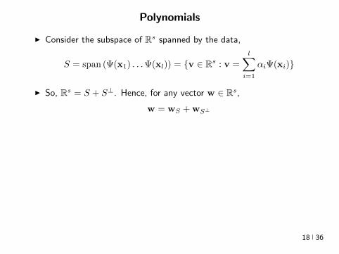
Polynomials
I Consider the subspace of Rs spanned by the data
S = span (Ψ(x1) Ψ(xl)) = v isin Rs v =
lsumi=1
αiΨ(xi)
I So Rs = S + Sperp Hence for any vector w isin Rs
w = wS + wSperp
I The search of a minimizer can be reduced to S because
lsumi=1
V (wTΨ(xi)) + λw22 gelsumi=1
V (wTSΨ(xi)) + λwS22 + wperpS 22
gelsumi=1
V (wTSΨ(xi)) + λwS22 (2)
I Argument holds for any loss (convex or non-convex additive or not)but needs orthogonality (l2 regularizer) [Representer Theorem]
18 36
Polynomials
I Consider the subspace of Rs spanned by the data
S = span (Ψ(x1) Ψ(xl)) = v isin Rs v =
lsumi=1
αiΨ(xi)
I So Rs = S + Sperp Hence for any vector w isin Rs
w = wS + wSperp
I The search of a minimizer can be reduced to S because
lsumi=1
V (wTΨ(xi)) + λw22 gelsumi=1
V (wTSΨ(xi)) + λwS22 + wperpS 22
gelsumi=1
V (wTSΨ(xi)) + λwS22 (2)
I Argument holds for any loss (convex or non-convex additive or not)but needs orthogonality (l2 regularizer) [Representer Theorem]
18 36
Polynomials
I Consider the subspace of Rs spanned by the data
S = span (Ψ(x1) Ψ(xl)) = v isin Rs v =
lsumi=1
αiΨ(xi)
I So Rs = S + Sperp Hence for any vector w isin Rs
w = wS + wSperp
I The search of a minimizer can be reduced to S because
lsumi=1
V (wTΨ(xi)) + λw22 gelsumi=1
V (wTSΨ(xi)) + λwS22 + wperpS 22
gelsumi=1
V (wTSΨ(xi)) + λwS22 (2)
I Argument holds for any loss (convex or non-convex additive or not)but needs orthogonality (l2 regularizer) [Representer Theorem]
18 36
Polynomials
I Hence w =sumli=1 βiΨ(xi) isin S for β isin Rl and so we can solve
arg minwisinRd
lsumi=1
(yi minuswTΨ(xi))2 + λw22
arg minβisinRl
lsumj=1
(yj minus
lsumi=1
βiΨ(xi)TΨ(xj)
)2
+ λ
lsumij=1
βiβjΨ(xi)TΨ(xj)
arg minβisinRl
lsumj=1
(yj minus (Gβ)j
)2+ λβTGβ
Gij = Ψ(xi)TΨ(xj)
β = (G + λId)minus1
y
I O(l3 + sl2) training time - O(s3) cost eliminatedI Inference time (O(s) or O(ls))
f(x) = wTΨ(x) =
lsumi=1
βiΨ(xi)TΨ(x)
19 36
Polynomials
I Multinomial Theorem
(z1 + z2 + + zn)d =sum
α|α|=d
(d
α
)zα
I Implicit computation of inner products
Ψ(x)TΨ(xprime) =
ssumi=1
(d
α
)xαxprime
α=
ssumi=1
(d
α
)xα11 xαnn x
primeα11 x
primeαnn
=
ssumi=1
(d
α
)(x1x
prime1)α1(x2x
prime2)α2 (xnx
primen)αn
= (x1xprime1 + xnx
primen)d
= (xTxprime)d
I O(l3 + l2n) training and O(ln) predicting speedI Complexity coming from s has been completely eliminated ()
[Kernel Trick]
20 36
Polynomials Algorithm
I Algorithm
ndash Start with k X times X 7rarr R k(xxprime) = (xTxprime + 1)d
ndash Construct Gram matrix Gij = k(xixj) on the training samplesndash Solve β = (G + λId)minus1 yndash Return f(x) =
sumli=1 βik(xix)
I f is the optimal degree-d polynomial solving the learning problemin complexity independent of d
I What other forms of k correspond to linear learning inhigh-dimensional nonlinear embeddings of the data
21 36
Symmetric positive semi-definite functions
I Definition A function k X times X 7rarr R is psd if for any finitecollection of points x1 xl the l times l Gram matrix
Gij = k(xixj)
is positive semi-definite ie for any vector β isin Rl
βTGβ =sumij
βiβjk(xixj) ge 0
I Theorem[Mercer] If k is symmetric psd X is compact subset ofRn then it admits an eigenfunction decomposition
k(xxprime) =
Nsumi=1
λiφj(x)φj(xprime) = 〈Ψ(x)Ψ(xprime)〉l2
Ψ(x) = [ radicλjφ(x) ]T (3)
I Feature map associated with a kernel is not uniqueI Functional generalization of positive semi-definite matrices
22 36
Kernels
I Lineark(xxprime) = xTxprime
I Polynomialk(xxprime) = (xTxprime + 1)d
I Gaussian s =infin Universal
k(xxprime) = eminusxminusxprime2
2σ2
I Conic combinations
k(xxprime) = α1k1(xxprime) + α2k2(xxprime)
I Elementwise products
k(xxprime) = k1(xxprime)k2(xxprime)
I Kernels on discrete sets strings graphs sequences shapes
23 36
Gaussian Kernel is Positive Definite
I Exponential
eβxTxprime = 1 + βxTxprime +
β2
2(xTy)2 +
β3
3(xTy)3 +
I For any function f Rn 7rarr R psd function k the following kernelis psd
kprime(xxprime) = f(x) (k(xxprime)) f(xprime)
Proofsumij
βiβjkprime(xixj) =
sumij
βiβjf(xi)k(xixj)f(xj) =sumij
βprimeiβprimejk(xixj) ge 0
I Gaussian Kernel
k(xxprime) = eminusxminusxprime22
2σ2
= eminusx222σ2
(e
2xT xprime2σ2
)eminusxprime222σ2 (4)
24 36
The Mathematical Naturalness of Kernel Methods
I Data X isin Rd Models isin H X 7rarr R
I Geometry in H inner product 〈middot middot〉H norm middot H (Hilbert Spaces)I Theorem All nice Hilbert spaces are generated by a symmetric
positive definite function (the kernel) k(xxprime) on X times XI if f g isin H close ie f minus gH small then f(x) g(x) close forallx isin X I Reproducing Kernel Hilbert Spaces (RKHSs) Hilbert space H
that admit a reproducing kernel ie a function k(xxprime) satisfying
(i) forallx isin X k(middotx) isin H(ii) 〈f k(middotx)〉H = f(x)
I Reproducing kernels are symmetric psdsumij
βiβjk(xixj) = 〈sumi
βik(middotxi)sumi
βik(middotxi)〉H
= sumi
βik(middotxi)2H ge 0 (5)
I (Moore-Aronsjan 1950) Symmetric psd functions arereproducing kernels for some (unique) RKHS Hk
25 36
The Mathematical Naturalness of Kernel Methods
I Data X isin Rd Models isin H X 7rarr RI Geometry in H inner product 〈middot middot〉H norm middot H (Hilbert Spaces)
I Theorem All nice Hilbert spaces are generated by a symmetricpositive definite function (the kernel) k(xxprime) on X times X
I if f g isin H close ie f minus gH small then f(x) g(x) close forallx isin X I Reproducing Kernel Hilbert Spaces (RKHSs) Hilbert space H
that admit a reproducing kernel ie a function k(xxprime) satisfying
(i) forallx isin X k(middotx) isin H(ii) 〈f k(middotx)〉H = f(x)
I Reproducing kernels are symmetric psdsumij
βiβjk(xixj) = 〈sumi
βik(middotxi)sumi
βik(middotxi)〉H
= sumi
βik(middotxi)2H ge 0 (5)
I (Moore-Aronsjan 1950) Symmetric psd functions arereproducing kernels for some (unique) RKHS Hk
25 36
The Mathematical Naturalness of Kernel Methods
I Data X isin Rd Models isin H X 7rarr RI Geometry in H inner product 〈middot middot〉H norm middot H (Hilbert Spaces)I Theorem All nice Hilbert spaces are generated by a symmetric
positive definite function (the kernel) k(xxprime) on X times XI if f g isin H close ie f minus gH small then f(x) g(x) close forallx isin X
I Reproducing Kernel Hilbert Spaces (RKHSs) Hilbert space Hthat admit a reproducing kernel ie a function k(xxprime) satisfying
(i) forallx isin X k(middotx) isin H(ii) 〈f k(middotx)〉H = f(x)
I Reproducing kernels are symmetric psdsumij
βiβjk(xixj) = 〈sumi
βik(middotxi)sumi
βik(middotxi)〉H
= sumi
βik(middotxi)2H ge 0 (5)
I (Moore-Aronsjan 1950) Symmetric psd functions arereproducing kernels for some (unique) RKHS Hk
25 36
The Mathematical Naturalness of Kernel Methods
I Data X isin Rd Models isin H X 7rarr RI Geometry in H inner product 〈middot middot〉H norm middot H (Hilbert Spaces)I Theorem All nice Hilbert spaces are generated by a symmetric
positive definite function (the kernel) k(xxprime) on X times XI if f g isin H close ie f minus gH small then f(x) g(x) close forallx isin X I Reproducing Kernel Hilbert Spaces (RKHSs) Hilbert space H
that admit a reproducing kernel ie a function k(xxprime) satisfying
(i) forallx isin X k(middotx) isin H(ii) 〈f k(middotx)〉H = f(x)
I Reproducing kernels are symmetric psdsumij
βiβjk(xixj) = 〈sumi
βik(middotxi)sumi
βik(middotxi)〉H
= sumi
βik(middotxi)2H ge 0 (5)
I (Moore-Aronsjan 1950) Symmetric psd functions arereproducing kernels for some (unique) RKHS Hk
25 36
The Mathematical Naturalness of Kernel Methods
I Data X isin Rd Models isin H X 7rarr RI Geometry in H inner product 〈middot middot〉H norm middot H (Hilbert Spaces)I Theorem All nice Hilbert spaces are generated by a symmetric
positive definite function (the kernel) k(xxprime) on X times XI if f g isin H close ie f minus gH small then f(x) g(x) close forallx isin X I Reproducing Kernel Hilbert Spaces (RKHSs) Hilbert space H
that admit a reproducing kernel ie a function k(xxprime) satisfying
(i) forallx isin X k(middotx) isin H(ii) 〈f k(middotx)〉H = f(x)
I Reproducing kernels are symmetric psdsumij
βiβjk(xixj) = 〈sumi
βik(middotxi)sumi
βik(middotxi)〉H
= sumi
βik(middotxi)2H ge 0 (5)
I (Moore-Aronsjan 1950) Symmetric psd functions arereproducing kernels for some (unique) RKHS Hk 25 36
Kernel Methods Summary
I Symm pos def function k(x z) on input domain X sub Rd
I k hArr rich Reproducing Kernel Hilbert Space (RKHS) Hk ofreal-valued functions with inner product 〈middot middot〉k and norm middot k
I Regularized Risk Minimization hArr Linear models in an implicithigh-dimensional (often infinite-dimensional) feature space
f = arg minfisinHk
1
n
nsumi=1
V (yi f(xi)) + λf2Hk xi isin Rd
I Representer Theorem f(x) =sumni=1 αik(xxi)
26 36
Shallow and Deep Function Spaces
I What does it mean to understand a function space
ndash Linear f(x) = wTxw isin Rd
ndash Polynomial f(x) = wT Ψ(x)w isin Rs
ndash RKHS balls f isin Hk fk lt γ [like vM le 1]
I Shallow nets f(x) = wTσ(Wx) (w isin RdW isin Rs)ndash For srarrinfin W sim p σ(u) = eminusiu approximates Gaussian kernel
methodsndash Theorem [Bochner 1937] One-to-one correspondence between k
and a density p such that
k(x z) = ψ(xminus z) =
intRdeminusi(xminusz)Twp(w)dw asymp 1
s
ssumj=1
eminusi(xminusz)Twj
Gaussian kernel k(x z) = eminusxminusz22
2σ2 lArrrArr p = N (0 σminus2Id)ndash Similar integral approx relates ReLU to the arc-cosine kernelndash Optimization versus Randomization
27 36
Shallow and Deep Function Spaces
I What does it mean to understand a function space
ndash Linear f(x) = wTxw isin Rd
ndash Polynomial f(x) = wT Ψ(x)w isin Rs
ndash RKHS balls f isin Hk fk lt γ [like vM le 1]
I Shallow nets f(x) = wTσ(Wx) (w isin RdW isin Rs)ndash For srarrinfin W sim p σ(u) = eminusiu approximates Gaussian kernel
methodsndash Theorem [Bochner 1937] One-to-one correspondence between k
and a density p such that
k(x z) = ψ(xminus z) =
intRdeminusi(xminusz)Twp(w)dw asymp 1
s
ssumj=1
eminusi(xminusz)Twj
Gaussian kernel k(x z) = eminusxminusz22
2σ2 lArrrArr p = N (0 σminus2Id)ndash Similar integral approx relates ReLU to the arc-cosine kernelndash Optimization versus Randomization
27 36
Shallow and Deep Function Spaces
I What does it mean to understand a function space
ndash Linear f(x) = wTxw isin Rd
ndash Polynomial f(x) = wT Ψ(x)w isin Rs
ndash RKHS balls f isin Hk fk lt γ [like vM le 1]
I Shallow nets f(x) = wTσ(Wx) (w isin RdW isin Rs)ndash For srarrinfin W sim p σ(u) = eminusiu approximates Gaussian kernel
methodsndash Theorem [Bochner 1937] One-to-one correspondence between k
and a density p such that
k(x z) = ψ(xminus z) =
intRdeminusi(xminusz)Twp(w)dw asymp 1
s
ssumj=1
eminusi(xminusz)Twj
Gaussian kernel k(x z) = eminusxminusz22
2σ2 lArrrArr p = N (0 σminus2Id)ndash Similar integral approx relates ReLU to the arc-cosine kernelndash Optimization versus Randomization
27 36
Shallow and Deep Function Spaces
I What does it mean to understand a function space
ndash Linear f(x) = wTxw isin Rd
ndash Polynomial f(x) = wT Ψ(x)w isin Rs
ndash RKHS balls f isin Hk fk lt γ [like vM le 1]
I Shallow nets f(x) = wTσ(Wx) (w isin RdW isin Rs)
ndash For srarrinfin W sim p σ(u) = eminusiu approximates Gaussian kernelmethods
ndash Theorem [Bochner 1937] One-to-one correspondence between kand a density p such that
k(x z) = ψ(xminus z) =
intRdeminusi(xminusz)Twp(w)dw asymp 1
s
ssumj=1
eminusi(xminusz)Twj
Gaussian kernel k(x z) = eminusxminusz22
2σ2 lArrrArr p = N (0 σminus2Id)ndash Similar integral approx relates ReLU to the arc-cosine kernelndash Optimization versus Randomization
27 36
Shallow and Deep Function Spaces
I What does it mean to understand a function space
ndash Linear f(x) = wTxw isin Rd
ndash Polynomial f(x) = wT Ψ(x)w isin Rs
ndash RKHS balls f isin Hk fk lt γ [like vM le 1]
I Shallow nets f(x) = wTσ(Wx) (w isin RdW isin Rs)ndash For srarrinfin W sim p σ(u) = eminusiu approximates Gaussian kernel
methodsndash Theorem [Bochner 1937] One-to-one correspondence between k
and a density p such that
k(x z) = ψ(xminus z) =
intRdeminusi(xminusz)Twp(w)dw asymp 1
s
ssumj=1
eminusi(xminusz)Twj
Gaussian kernel k(x z) = eminusxminusz22
2σ2 lArrrArr p = N (0 σminus2Id)ndash Similar integral approx relates ReLU to the arc-cosine kernelndash Optimization versus Randomization
27 36
Expressivity of Deep Nets Linear Regions
I The ReLU map f(x) = max(Wx 0)W isin Rwtimesn is piecewise linear
I A piece is a connected region (a convex polytope) of Rd with sharedsparsity pattern in activations
I (Zaslavsky 1975) Number of linear regions formed by an arrangement of
s hyperplanes in d-dimensions in general position issumd
i=0
(si
)I Composition of ReLU maps is also piecewise linear
I (Raghu et al 2017 Pascano et al 2014 Montufar 2014) Number oflinear regions grows as O(wnd) for a composition of d ReLU maps(nrarr brarr brarr b rarr b) each of width w
I (Safran and Shamir 2017)
ndash 1[x le 1] x isin Rd ε-accurate 3-layer network with O(dε) neurons but cannot be approximated with
accuracy higher than O(1d4) using 2-layer networks unless width is exponential in d
28 36
Expressivity of Deep Nets Linear Regions
I The ReLU map f(x) = max(Wx 0)W isin Rwtimesn is piecewise linear
I A piece is a connected region (a convex polytope) of Rd with sharedsparsity pattern in activations
I (Zaslavsky 1975) Number of linear regions formed by an arrangement of
s hyperplanes in d-dimensions in general position issumd
i=0
(si
)I Composition of ReLU maps is also piecewise linear
I (Raghu et al 2017 Pascano et al 2014 Montufar 2014) Number oflinear regions grows as O(wnd) for a composition of d ReLU maps(nrarr brarr brarr b rarr b) each of width w
I (Safran and Shamir 2017)
ndash 1[x le 1] x isin Rd ε-accurate 3-layer network with O(dε) neurons but cannot be approximated with
accuracy higher than O(1d4) using 2-layer networks unless width is exponential in d
28 36
Expressivity of Deep Nets Linear Regions
I The ReLU map f(x) = max(Wx 0)W isin Rwtimesn is piecewise linear
I A piece is a connected region (a convex polytope) of Rd with sharedsparsity pattern in activations
I (Zaslavsky 1975) Number of linear regions formed by an arrangement of
s hyperplanes in d-dimensions in general position issumd
i=0
(si
)
I Composition of ReLU maps is also piecewise linear
I (Raghu et al 2017 Pascano et al 2014 Montufar 2014) Number oflinear regions grows as O(wnd) for a composition of d ReLU maps(nrarr brarr brarr b rarr b) each of width w
I (Safran and Shamir 2017)
ndash 1[x le 1] x isin Rd ε-accurate 3-layer network with O(dε) neurons but cannot be approximated with
accuracy higher than O(1d4) using 2-layer networks unless width is exponential in d
28 36
Expressivity of Deep Nets Linear Regions
I The ReLU map f(x) = max(Wx 0)W isin Rwtimesn is piecewise linear
I A piece is a connected region (a convex polytope) of Rd with sharedsparsity pattern in activations
I (Zaslavsky 1975) Number of linear regions formed by an arrangement of
s hyperplanes in d-dimensions in general position issumd
i=0
(si
)I Composition of ReLU maps is also piecewise linear
I (Raghu et al 2017 Pascano et al 2014 Montufar 2014) Number oflinear regions grows as O(wnd) for a composition of d ReLU maps(nrarr brarr brarr b rarr b) each of width w
I (Safran and Shamir 2017)
ndash 1[x le 1] x isin Rd ε-accurate 3-layer network with O(dε) neurons but cannot be approximated with
accuracy higher than O(1d4) using 2-layer networks unless width is exponential in d28 36
Expressivity of Deep Nets Trajectory Length
I (Raghu et al 2017) Trajectory Length (ldquogeneralized operator normrdquo)How much is a curve in the input space stretched by a layer in thenetwork
29 36
Expressivity of Deep Nets Trajectory Length
I (Raghu et al 2017) Trajectory Length (ldquogeneralized operator normrdquo)How much is a curve in the input space stretched by a layer in thenetwork
29 36
Expressivity and Generalization
I Expressiveness equiv capacity to fit random noise =rArr susceptibility tooverfitting (VC dimension Rademacher Complexity)
I Zhang et al 2017 Famous CNNs easily fit random labels
ndash Over-parameterized (n=12M psim 60M) but structuredndash Domain-knowledge baked in does not constraint expressiveness
I CNNs tend to generalize even without regularization (explicit and implicit)
I For linear regression SGD returns minimum norm solution
30 36
Expressivity and Generalization
I Expressiveness equiv capacity to fit random noise =rArr susceptibility tooverfitting (VC dimension Rademacher Complexity)
I Zhang et al 2017 Famous CNNs easily fit random labels
ndash Over-parameterized (n=12M psim 60M) but structuredndash Domain-knowledge baked in does not constraint expressiveness
I CNNs tend to generalize even without regularization (explicit and implicit)
I For linear regression SGD returns minimum norm solution
30 36
Expressivity and Generalization
I Expressiveness equiv capacity to fit random noise =rArr susceptibility tooverfitting (VC dimension Rademacher Complexity)
I Zhang et al 2017 Famous CNNs easily fit random labels
ndash Over-parameterized (n=12M psim 60M) but structuredndash Domain-knowledge baked in does not constraint expressiveness
I CNNs tend to generalize even without regularization (explicit and implicit)
I For linear regression SGD returns minimum norm solution
30 36
Optimization Landscape Symmetry and Saddle Points
I Folklore lots of equivalent good local minI Classification of critical points based on Hessian spectrumI Permutation and Scaling symmetries
I Thm [Lee et al 2016 Anadkumar Ge] For the short-step gradientmethod the basin of attraction of strict saddle points (atleast onenegative eigenvalue) has measure zero
31 36
Optimization Landscape Symmetry and Saddle Points
I Folklore lots of equivalent good local minI Classification of critical points based on Hessian spectrumI Permutation and Scaling symmetries
I Thm [Lee et al 2016 Anadkumar Ge] For the short-step gradientmethod the basin of attraction of strict saddle points (atleast onenegative eigenvalue) has measure zero
31 36
Optimization Landscape Symmetry and Saddle Points
I Folklore lots of equivalent good local minI Classification of critical points based on Hessian spectrumI Permutation and Scaling symmetries
I Thm [Lee et al 2016 Anadkumar Ge] For the short-step gradientmethod the basin of attraction of strict saddle points (atleast onenegative eigenvalue) has measure zero
31 36
Optimization Landscape Sharp Minima and Stability
Keskar et al 2017 On large-batch training for DL Generalization Gap and Sharp Minima
32 36
Deep Learning Computational Graphs TensorFlow
tensorfloworg
I Tensors-in Tensors-out
I Evergrowing list of Tensor-Ops (PythonC++)
f(xw)
[partf
partx
]T v
[partf
partw
]T v
I Automatic Differentiation Reverse mode
partxL
partxi=sumirarrj
partxL
partxj
partxj
partxi
33 36
Computational Graphs and TensorFlow
tensorfloworg
I SGD with minibatches
wk+1 = wk minus ηlsumi=1
partli
partw
∣∣∣wt
I Model Parallelism Assign independent paths tothreads GPUs
I Data Parallelism create Graph replicas on differentmachines
I Mobile TensorFlow
34 36
Computational Graphs and TensorFlow
tensorfloworg
35 36
Computational Graphs and TensorFlow
tensorfloworg
35 36
Computational Graphs and TensorFlow
tensorfloworg
35 36
Challenges and Opportunities
I Lots of fascinating unsolved problems
I Can you win Imagenet with Convex optimization
I Tools from polynomial optimization (global optimization deep-RL)
I Supervised to Semi-supervised to Unsupervised Learning
I Compact efficient real-time models (eliminateover-parametrization) for new form factors
I Exciting emerging world of Robotics Wearable ComputersIntelligent home devices Personal digital assistants
Google Internship Program
36 36
- anm0
- fdrm0
- fdrm5

Polynomials
I Consider the subspace of Rs spanned by the data
S = span (Ψ(x1) Ψ(xl)) = v isin Rs v =
lsumi=1
αiΨ(xi)
I So Rs = S + Sperp Hence for any vector w isin Rs
w = wS + wSperp
I The search of a minimizer can be reduced to S because
lsumi=1
V (wTΨ(xi)) + λw22 gelsumi=1
V (wTSΨ(xi)) + λwS22 + wperpS 22
gelsumi=1
V (wTSΨ(xi)) + λwS22 (2)
I Argument holds for any loss (convex or non-convex additive or not)but needs orthogonality (l2 regularizer) [Representer Theorem]
18 36
Polynomials
I Consider the subspace of Rs spanned by the data
S = span (Ψ(x1) Ψ(xl)) = v isin Rs v =
lsumi=1
αiΨ(xi)
I So Rs = S + Sperp Hence for any vector w isin Rs
w = wS + wSperp
I The search of a minimizer can be reduced to S because
lsumi=1
V (wTΨ(xi)) + λw22 gelsumi=1
V (wTSΨ(xi)) + λwS22 + wperpS 22
gelsumi=1
V (wTSΨ(xi)) + λwS22 (2)
I Argument holds for any loss (convex or non-convex additive or not)but needs orthogonality (l2 regularizer) [Representer Theorem]
18 36
Polynomials
I Hence w =sumli=1 βiΨ(xi) isin S for β isin Rl and so we can solve
arg minwisinRd
lsumi=1
(yi minuswTΨ(xi))2 + λw22
arg minβisinRl
lsumj=1
(yj minus
lsumi=1
βiΨ(xi)TΨ(xj)
)2
+ λ
lsumij=1
βiβjΨ(xi)TΨ(xj)
arg minβisinRl
lsumj=1
(yj minus (Gβ)j
)2+ λβTGβ
Gij = Ψ(xi)TΨ(xj)
β = (G + λId)minus1
y
I O(l3 + sl2) training time - O(s3) cost eliminatedI Inference time (O(s) or O(ls))
f(x) = wTΨ(x) =
lsumi=1
βiΨ(xi)TΨ(x)
19 36
Polynomials
I Multinomial Theorem
(z1 + z2 + + zn)d =sum
α|α|=d
(d
α
)zα
I Implicit computation of inner products
Ψ(x)TΨ(xprime) =
ssumi=1
(d
α
)xαxprime
α=
ssumi=1
(d
α
)xα11 xαnn x
primeα11 x
primeαnn
=
ssumi=1
(d
α
)(x1x
prime1)α1(x2x
prime2)α2 (xnx
primen)αn
= (x1xprime1 + xnx
primen)d
= (xTxprime)d
I O(l3 + l2n) training and O(ln) predicting speedI Complexity coming from s has been completely eliminated ()
[Kernel Trick]
20 36
Polynomials Algorithm
I Algorithm
ndash Start with k X times X 7rarr R k(xxprime) = (xTxprime + 1)d
ndash Construct Gram matrix Gij = k(xixj) on the training samplesndash Solve β = (G + λId)minus1 yndash Return f(x) =
sumli=1 βik(xix)
I f is the optimal degree-d polynomial solving the learning problemin complexity independent of d
I What other forms of k correspond to linear learning inhigh-dimensional nonlinear embeddings of the data
21 36
Symmetric positive semi-definite functions
I Definition A function k X times X 7rarr R is psd if for any finitecollection of points x1 xl the l times l Gram matrix
Gij = k(xixj)
is positive semi-definite ie for any vector β isin Rl
βTGβ =sumij
βiβjk(xixj) ge 0
I Theorem[Mercer] If k is symmetric psd X is compact subset ofRn then it admits an eigenfunction decomposition
k(xxprime) =
Nsumi=1
λiφj(x)φj(xprime) = 〈Ψ(x)Ψ(xprime)〉l2
Ψ(x) = [ radicλjφ(x) ]T (3)
I Feature map associated with a kernel is not uniqueI Functional generalization of positive semi-definite matrices
22 36
Kernels
I Lineark(xxprime) = xTxprime
I Polynomialk(xxprime) = (xTxprime + 1)d
I Gaussian s =infin Universal
k(xxprime) = eminusxminusxprime2
2σ2
I Conic combinations
k(xxprime) = α1k1(xxprime) + α2k2(xxprime)
I Elementwise products
k(xxprime) = k1(xxprime)k2(xxprime)
I Kernels on discrete sets strings graphs sequences shapes
23 36
Gaussian Kernel is Positive Definite
I Exponential
eβxTxprime = 1 + βxTxprime +
β2
2(xTy)2 +
β3
3(xTy)3 +
I For any function f Rn 7rarr R psd function k the following kernelis psd
kprime(xxprime) = f(x) (k(xxprime)) f(xprime)
Proofsumij
βiβjkprime(xixj) =
sumij
βiβjf(xi)k(xixj)f(xj) =sumij
βprimeiβprimejk(xixj) ge 0
I Gaussian Kernel
k(xxprime) = eminusxminusxprime22
2σ2
= eminusx222σ2
(e
2xT xprime2σ2
)eminusxprime222σ2 (4)
24 36
The Mathematical Naturalness of Kernel Methods
I Data X isin Rd Models isin H X 7rarr R
I Geometry in H inner product 〈middot middot〉H norm middot H (Hilbert Spaces)I Theorem All nice Hilbert spaces are generated by a symmetric
positive definite function (the kernel) k(xxprime) on X times XI if f g isin H close ie f minus gH small then f(x) g(x) close forallx isin X I Reproducing Kernel Hilbert Spaces (RKHSs) Hilbert space H
that admit a reproducing kernel ie a function k(xxprime) satisfying
(i) forallx isin X k(middotx) isin H(ii) 〈f k(middotx)〉H = f(x)
I Reproducing kernels are symmetric psdsumij
βiβjk(xixj) = 〈sumi
βik(middotxi)sumi
βik(middotxi)〉H
= sumi
βik(middotxi)2H ge 0 (5)
I (Moore-Aronsjan 1950) Symmetric psd functions arereproducing kernels for some (unique) RKHS Hk
25 36
The Mathematical Naturalness of Kernel Methods
I Data X isin Rd Models isin H X 7rarr RI Geometry in H inner product 〈middot middot〉H norm middot H (Hilbert Spaces)
I Theorem All nice Hilbert spaces are generated by a symmetricpositive definite function (the kernel) k(xxprime) on X times X
I if f g isin H close ie f minus gH small then f(x) g(x) close forallx isin X I Reproducing Kernel Hilbert Spaces (RKHSs) Hilbert space H
that admit a reproducing kernel ie a function k(xxprime) satisfying
(i) forallx isin X k(middotx) isin H(ii) 〈f k(middotx)〉H = f(x)
I Reproducing kernels are symmetric psdsumij
βiβjk(xixj) = 〈sumi
βik(middotxi)sumi
βik(middotxi)〉H
= sumi
βik(middotxi)2H ge 0 (5)
I (Moore-Aronsjan 1950) Symmetric psd functions arereproducing kernels for some (unique) RKHS Hk
25 36
The Mathematical Naturalness of Kernel Methods
I Data X isin Rd Models isin H X 7rarr RI Geometry in H inner product 〈middot middot〉H norm middot H (Hilbert Spaces)I Theorem All nice Hilbert spaces are generated by a symmetric
positive definite function (the kernel) k(xxprime) on X times XI if f g isin H close ie f minus gH small then f(x) g(x) close forallx isin X
I Reproducing Kernel Hilbert Spaces (RKHSs) Hilbert space Hthat admit a reproducing kernel ie a function k(xxprime) satisfying
(i) forallx isin X k(middotx) isin H(ii) 〈f k(middotx)〉H = f(x)
I Reproducing kernels are symmetric psdsumij
βiβjk(xixj) = 〈sumi
βik(middotxi)sumi
βik(middotxi)〉H
= sumi
βik(middotxi)2H ge 0 (5)
I (Moore-Aronsjan 1950) Symmetric psd functions arereproducing kernels for some (unique) RKHS Hk
25 36
The Mathematical Naturalness of Kernel Methods
I Data X isin Rd Models isin H X 7rarr RI Geometry in H inner product 〈middot middot〉H norm middot H (Hilbert Spaces)I Theorem All nice Hilbert spaces are generated by a symmetric
positive definite function (the kernel) k(xxprime) on X times XI if f g isin H close ie f minus gH small then f(x) g(x) close forallx isin X I Reproducing Kernel Hilbert Spaces (RKHSs) Hilbert space H
that admit a reproducing kernel ie a function k(xxprime) satisfying
(i) forallx isin X k(middotx) isin H(ii) 〈f k(middotx)〉H = f(x)
I Reproducing kernels are symmetric psdsumij
βiβjk(xixj) = 〈sumi
βik(middotxi)sumi
βik(middotxi)〉H
= sumi
βik(middotxi)2H ge 0 (5)
I (Moore-Aronsjan 1950) Symmetric psd functions arereproducing kernels for some (unique) RKHS Hk
25 36
The Mathematical Naturalness of Kernel Methods
I Data X isin Rd Models isin H X 7rarr RI Geometry in H inner product 〈middot middot〉H norm middot H (Hilbert Spaces)I Theorem All nice Hilbert spaces are generated by a symmetric
positive definite function (the kernel) k(xxprime) on X times XI if f g isin H close ie f minus gH small then f(x) g(x) close forallx isin X I Reproducing Kernel Hilbert Spaces (RKHSs) Hilbert space H
that admit a reproducing kernel ie a function k(xxprime) satisfying
(i) forallx isin X k(middotx) isin H(ii) 〈f k(middotx)〉H = f(x)
I Reproducing kernels are symmetric psdsumij
βiβjk(xixj) = 〈sumi
βik(middotxi)sumi
βik(middotxi)〉H
= sumi
βik(middotxi)2H ge 0 (5)
I (Moore-Aronsjan 1950) Symmetric psd functions arereproducing kernels for some (unique) RKHS Hk 25 36
Kernel Methods Summary
I Symm pos def function k(x z) on input domain X sub Rd
I k hArr rich Reproducing Kernel Hilbert Space (RKHS) Hk ofreal-valued functions with inner product 〈middot middot〉k and norm middot k
I Regularized Risk Minimization hArr Linear models in an implicithigh-dimensional (often infinite-dimensional) feature space
f = arg minfisinHk
1
n
nsumi=1
V (yi f(xi)) + λf2Hk xi isin Rd
I Representer Theorem f(x) =sumni=1 αik(xxi)
26 36
Shallow and Deep Function Spaces
I What does it mean to understand a function space
ndash Linear f(x) = wTxw isin Rd
ndash Polynomial f(x) = wT Ψ(x)w isin Rs
ndash RKHS balls f isin Hk fk lt γ [like vM le 1]
I Shallow nets f(x) = wTσ(Wx) (w isin RdW isin Rs)ndash For srarrinfin W sim p σ(u) = eminusiu approximates Gaussian kernel
methodsndash Theorem [Bochner 1937] One-to-one correspondence between k
and a density p such that
k(x z) = ψ(xminus z) =
intRdeminusi(xminusz)Twp(w)dw asymp 1
s
ssumj=1
eminusi(xminusz)Twj
Gaussian kernel k(x z) = eminusxminusz22
2σ2 lArrrArr p = N (0 σminus2Id)ndash Similar integral approx relates ReLU to the arc-cosine kernelndash Optimization versus Randomization
27 36
Shallow and Deep Function Spaces
I What does it mean to understand a function space
ndash Linear f(x) = wTxw isin Rd
ndash Polynomial f(x) = wT Ψ(x)w isin Rs
ndash RKHS balls f isin Hk fk lt γ [like vM le 1]
I Shallow nets f(x) = wTσ(Wx) (w isin RdW isin Rs)ndash For srarrinfin W sim p σ(u) = eminusiu approximates Gaussian kernel
methodsndash Theorem [Bochner 1937] One-to-one correspondence between k
and a density p such that
k(x z) = ψ(xminus z) =
intRdeminusi(xminusz)Twp(w)dw asymp 1
s
ssumj=1
eminusi(xminusz)Twj
Gaussian kernel k(x z) = eminusxminusz22
2σ2 lArrrArr p = N (0 σminus2Id)ndash Similar integral approx relates ReLU to the arc-cosine kernelndash Optimization versus Randomization
27 36
Shallow and Deep Function Spaces
I What does it mean to understand a function space
ndash Linear f(x) = wTxw isin Rd
ndash Polynomial f(x) = wT Ψ(x)w isin Rs
ndash RKHS balls f isin Hk fk lt γ [like vM le 1]
I Shallow nets f(x) = wTσ(Wx) (w isin RdW isin Rs)ndash For srarrinfin W sim p σ(u) = eminusiu approximates Gaussian kernel
methodsndash Theorem [Bochner 1937] One-to-one correspondence between k
and a density p such that
k(x z) = ψ(xminus z) =
intRdeminusi(xminusz)Twp(w)dw asymp 1
s
ssumj=1
eminusi(xminusz)Twj
Gaussian kernel k(x z) = eminusxminusz22
2σ2 lArrrArr p = N (0 σminus2Id)ndash Similar integral approx relates ReLU to the arc-cosine kernelndash Optimization versus Randomization
27 36
Shallow and Deep Function Spaces
I What does it mean to understand a function space
ndash Linear f(x) = wTxw isin Rd
ndash Polynomial f(x) = wT Ψ(x)w isin Rs
ndash RKHS balls f isin Hk fk lt γ [like vM le 1]
I Shallow nets f(x) = wTσ(Wx) (w isin RdW isin Rs)
ndash For srarrinfin W sim p σ(u) = eminusiu approximates Gaussian kernelmethods
ndash Theorem [Bochner 1937] One-to-one correspondence between kand a density p such that
k(x z) = ψ(xminus z) =
intRdeminusi(xminusz)Twp(w)dw asymp 1
s
ssumj=1
eminusi(xminusz)Twj
Gaussian kernel k(x z) = eminusxminusz22
2σ2 lArrrArr p = N (0 σminus2Id)ndash Similar integral approx relates ReLU to the arc-cosine kernelndash Optimization versus Randomization
27 36
Shallow and Deep Function Spaces
I What does it mean to understand a function space
ndash Linear f(x) = wTxw isin Rd
ndash Polynomial f(x) = wT Ψ(x)w isin Rs
ndash RKHS balls f isin Hk fk lt γ [like vM le 1]
I Shallow nets f(x) = wTσ(Wx) (w isin RdW isin Rs)ndash For srarrinfin W sim p σ(u) = eminusiu approximates Gaussian kernel
methodsndash Theorem [Bochner 1937] One-to-one correspondence between k
and a density p such that
k(x z) = ψ(xminus z) =
intRdeminusi(xminusz)Twp(w)dw asymp 1
s
ssumj=1
eminusi(xminusz)Twj
Gaussian kernel k(x z) = eminusxminusz22
2σ2 lArrrArr p = N (0 σminus2Id)ndash Similar integral approx relates ReLU to the arc-cosine kernelndash Optimization versus Randomization
27 36
Expressivity of Deep Nets Linear Regions
I The ReLU map f(x) = max(Wx 0)W isin Rwtimesn is piecewise linear
I A piece is a connected region (a convex polytope) of Rd with sharedsparsity pattern in activations
I (Zaslavsky 1975) Number of linear regions formed by an arrangement of
s hyperplanes in d-dimensions in general position issumd
i=0
(si
)I Composition of ReLU maps is also piecewise linear
I (Raghu et al 2017 Pascano et al 2014 Montufar 2014) Number oflinear regions grows as O(wnd) for a composition of d ReLU maps(nrarr brarr brarr b rarr b) each of width w
I (Safran and Shamir 2017)
ndash 1[x le 1] x isin Rd ε-accurate 3-layer network with O(dε) neurons but cannot be approximated with
accuracy higher than O(1d4) using 2-layer networks unless width is exponential in d
28 36
Expressivity of Deep Nets Linear Regions
I The ReLU map f(x) = max(Wx 0)W isin Rwtimesn is piecewise linear
I A piece is a connected region (a convex polytope) of Rd with sharedsparsity pattern in activations
I (Zaslavsky 1975) Number of linear regions formed by an arrangement of
s hyperplanes in d-dimensions in general position issumd
i=0
(si
)I Composition of ReLU maps is also piecewise linear
I (Raghu et al 2017 Pascano et al 2014 Montufar 2014) Number oflinear regions grows as O(wnd) for a composition of d ReLU maps(nrarr brarr brarr b rarr b) each of width w
I (Safran and Shamir 2017)
ndash 1[x le 1] x isin Rd ε-accurate 3-layer network with O(dε) neurons but cannot be approximated with
accuracy higher than O(1d4) using 2-layer networks unless width is exponential in d
28 36
Expressivity of Deep Nets Linear Regions
I The ReLU map f(x) = max(Wx 0)W isin Rwtimesn is piecewise linear
I A piece is a connected region (a convex polytope) of Rd with sharedsparsity pattern in activations
I (Zaslavsky 1975) Number of linear regions formed by an arrangement of
s hyperplanes in d-dimensions in general position issumd
i=0
(si
)
I Composition of ReLU maps is also piecewise linear
I (Raghu et al 2017 Pascano et al 2014 Montufar 2014) Number oflinear regions grows as O(wnd) for a composition of d ReLU maps(nrarr brarr brarr b rarr b) each of width w
I (Safran and Shamir 2017)
ndash 1[x le 1] x isin Rd ε-accurate 3-layer network with O(dε) neurons but cannot be approximated with
accuracy higher than O(1d4) using 2-layer networks unless width is exponential in d
28 36
Expressivity of Deep Nets Linear Regions
I The ReLU map f(x) = max(Wx 0)W isin Rwtimesn is piecewise linear
I A piece is a connected region (a convex polytope) of Rd with sharedsparsity pattern in activations
I (Zaslavsky 1975) Number of linear regions formed by an arrangement of
s hyperplanes in d-dimensions in general position issumd
i=0
(si
)I Composition of ReLU maps is also piecewise linear
I (Raghu et al 2017 Pascano et al 2014 Montufar 2014) Number oflinear regions grows as O(wnd) for a composition of d ReLU maps(nrarr brarr brarr b rarr b) each of width w
I (Safran and Shamir 2017)
ndash 1[x le 1] x isin Rd ε-accurate 3-layer network with O(dε) neurons but cannot be approximated with
accuracy higher than O(1d4) using 2-layer networks unless width is exponential in d28 36
Expressivity of Deep Nets Trajectory Length
I (Raghu et al 2017) Trajectory Length (ldquogeneralized operator normrdquo)How much is a curve in the input space stretched by a layer in thenetwork
29 36
Expressivity of Deep Nets Trajectory Length
I (Raghu et al 2017) Trajectory Length (ldquogeneralized operator normrdquo)How much is a curve in the input space stretched by a layer in thenetwork
29 36
Expressivity and Generalization
I Expressiveness equiv capacity to fit random noise =rArr susceptibility tooverfitting (VC dimension Rademacher Complexity)
I Zhang et al 2017 Famous CNNs easily fit random labels
ndash Over-parameterized (n=12M psim 60M) but structuredndash Domain-knowledge baked in does not constraint expressiveness
I CNNs tend to generalize even without regularization (explicit and implicit)
I For linear regression SGD returns minimum norm solution
30 36
Expressivity and Generalization
I Expressiveness equiv capacity to fit random noise =rArr susceptibility tooverfitting (VC dimension Rademacher Complexity)
I Zhang et al 2017 Famous CNNs easily fit random labels
ndash Over-parameterized (n=12M psim 60M) but structuredndash Domain-knowledge baked in does not constraint expressiveness
I CNNs tend to generalize even without regularization (explicit and implicit)
I For linear regression SGD returns minimum norm solution
30 36
Expressivity and Generalization
I Expressiveness equiv capacity to fit random noise =rArr susceptibility tooverfitting (VC dimension Rademacher Complexity)
I Zhang et al 2017 Famous CNNs easily fit random labels
ndash Over-parameterized (n=12M psim 60M) but structuredndash Domain-knowledge baked in does not constraint expressiveness
I CNNs tend to generalize even without regularization (explicit and implicit)
I For linear regression SGD returns minimum norm solution
30 36
Optimization Landscape Symmetry and Saddle Points
I Folklore lots of equivalent good local minI Classification of critical points based on Hessian spectrumI Permutation and Scaling symmetries
I Thm [Lee et al 2016 Anadkumar Ge] For the short-step gradientmethod the basin of attraction of strict saddle points (atleast onenegative eigenvalue) has measure zero
31 36
Optimization Landscape Symmetry and Saddle Points
I Folklore lots of equivalent good local minI Classification of critical points based on Hessian spectrumI Permutation and Scaling symmetries
I Thm [Lee et al 2016 Anadkumar Ge] For the short-step gradientmethod the basin of attraction of strict saddle points (atleast onenegative eigenvalue) has measure zero
31 36
Optimization Landscape Symmetry and Saddle Points
I Folklore lots of equivalent good local minI Classification of critical points based on Hessian spectrumI Permutation and Scaling symmetries
I Thm [Lee et al 2016 Anadkumar Ge] For the short-step gradientmethod the basin of attraction of strict saddle points (atleast onenegative eigenvalue) has measure zero
31 36
Optimization Landscape Sharp Minima and Stability
Keskar et al 2017 On large-batch training for DL Generalization Gap and Sharp Minima
32 36
Deep Learning Computational Graphs TensorFlow
tensorfloworg
I Tensors-in Tensors-out
I Evergrowing list of Tensor-Ops (PythonC++)
f(xw)
[partf
partx
]T v
[partf
partw
]T v
I Automatic Differentiation Reverse mode
partxL
partxi=sumirarrj
partxL
partxj
partxj
partxi
33 36
Computational Graphs and TensorFlow
tensorfloworg
I SGD with minibatches
wk+1 = wk minus ηlsumi=1
partli
partw
∣∣∣wt
I Model Parallelism Assign independent paths tothreads GPUs
I Data Parallelism create Graph replicas on differentmachines
I Mobile TensorFlow
34 36
Computational Graphs and TensorFlow
tensorfloworg
35 36
Computational Graphs and TensorFlow
tensorfloworg
35 36
Computational Graphs and TensorFlow
tensorfloworg
35 36
Challenges and Opportunities
I Lots of fascinating unsolved problems
I Can you win Imagenet with Convex optimization
I Tools from polynomial optimization (global optimization deep-RL)
I Supervised to Semi-supervised to Unsupervised Learning
I Compact efficient real-time models (eliminateover-parametrization) for new form factors
I Exciting emerging world of Robotics Wearable ComputersIntelligent home devices Personal digital assistants
Google Internship Program
36 36
- anm0
- fdrm0
- fdrm5
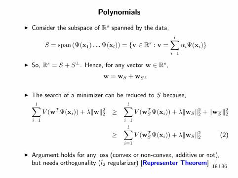
Polynomials
I Consider the subspace of Rs spanned by the data
S = span (Ψ(x1) Ψ(xl)) = v isin Rs v =
lsumi=1
αiΨ(xi)
I So Rs = S + Sperp Hence for any vector w isin Rs
w = wS + wSperp
I The search of a minimizer can be reduced to S because
lsumi=1
V (wTΨ(xi)) + λw22 gelsumi=1
V (wTSΨ(xi)) + λwS22 + wperpS 22
gelsumi=1
V (wTSΨ(xi)) + λwS22 (2)
I Argument holds for any loss (convex or non-convex additive or not)but needs orthogonality (l2 regularizer) [Representer Theorem]
18 36
Polynomials
I Hence w =sumli=1 βiΨ(xi) isin S for β isin Rl and so we can solve
arg minwisinRd
lsumi=1
(yi minuswTΨ(xi))2 + λw22
arg minβisinRl
lsumj=1
(yj minus
lsumi=1
βiΨ(xi)TΨ(xj)
)2
+ λ
lsumij=1
βiβjΨ(xi)TΨ(xj)
arg minβisinRl
lsumj=1
(yj minus (Gβ)j
)2+ λβTGβ
Gij = Ψ(xi)TΨ(xj)
β = (G + λId)minus1
y
I O(l3 + sl2) training time - O(s3) cost eliminatedI Inference time (O(s) or O(ls))
f(x) = wTΨ(x) =
lsumi=1
βiΨ(xi)TΨ(x)
19 36
Polynomials
I Multinomial Theorem
(z1 + z2 + + zn)d =sum
α|α|=d
(d
α
)zα
I Implicit computation of inner products
Ψ(x)TΨ(xprime) =
ssumi=1
(d
α
)xαxprime
α=
ssumi=1
(d
α
)xα11 xαnn x
primeα11 x
primeαnn
=
ssumi=1
(d
α
)(x1x
prime1)α1(x2x
prime2)α2 (xnx
primen)αn
= (x1xprime1 + xnx
primen)d
= (xTxprime)d
I O(l3 + l2n) training and O(ln) predicting speedI Complexity coming from s has been completely eliminated ()
[Kernel Trick]
20 36
Polynomials Algorithm
I Algorithm
ndash Start with k X times X 7rarr R k(xxprime) = (xTxprime + 1)d
ndash Construct Gram matrix Gij = k(xixj) on the training samplesndash Solve β = (G + λId)minus1 yndash Return f(x) =
sumli=1 βik(xix)
I f is the optimal degree-d polynomial solving the learning problemin complexity independent of d
I What other forms of k correspond to linear learning inhigh-dimensional nonlinear embeddings of the data
21 36
Symmetric positive semi-definite functions
I Definition A function k X times X 7rarr R is psd if for any finitecollection of points x1 xl the l times l Gram matrix
Gij = k(xixj)
is positive semi-definite ie for any vector β isin Rl
βTGβ =sumij
βiβjk(xixj) ge 0
I Theorem[Mercer] If k is symmetric psd X is compact subset ofRn then it admits an eigenfunction decomposition
k(xxprime) =
Nsumi=1
λiφj(x)φj(xprime) = 〈Ψ(x)Ψ(xprime)〉l2
Ψ(x) = [ radicλjφ(x) ]T (3)
I Feature map associated with a kernel is not uniqueI Functional generalization of positive semi-definite matrices
22 36
Kernels
I Lineark(xxprime) = xTxprime
I Polynomialk(xxprime) = (xTxprime + 1)d
I Gaussian s =infin Universal
k(xxprime) = eminusxminusxprime2
2σ2
I Conic combinations
k(xxprime) = α1k1(xxprime) + α2k2(xxprime)
I Elementwise products
k(xxprime) = k1(xxprime)k2(xxprime)
I Kernels on discrete sets strings graphs sequences shapes
23 36
Gaussian Kernel is Positive Definite
I Exponential
eβxTxprime = 1 + βxTxprime +
β2
2(xTy)2 +
β3
3(xTy)3 +
I For any function f Rn 7rarr R psd function k the following kernelis psd
kprime(xxprime) = f(x) (k(xxprime)) f(xprime)
Proofsumij
βiβjkprime(xixj) =
sumij
βiβjf(xi)k(xixj)f(xj) =sumij
βprimeiβprimejk(xixj) ge 0
I Gaussian Kernel
k(xxprime) = eminusxminusxprime22
2σ2
= eminusx222σ2
(e
2xT xprime2σ2
)eminusxprime222σ2 (4)
24 36
The Mathematical Naturalness of Kernel Methods
I Data X isin Rd Models isin H X 7rarr R
I Geometry in H inner product 〈middot middot〉H norm middot H (Hilbert Spaces)I Theorem All nice Hilbert spaces are generated by a symmetric
positive definite function (the kernel) k(xxprime) on X times XI if f g isin H close ie f minus gH small then f(x) g(x) close forallx isin X I Reproducing Kernel Hilbert Spaces (RKHSs) Hilbert space H
that admit a reproducing kernel ie a function k(xxprime) satisfying
(i) forallx isin X k(middotx) isin H(ii) 〈f k(middotx)〉H = f(x)
I Reproducing kernels are symmetric psdsumij
βiβjk(xixj) = 〈sumi
βik(middotxi)sumi
βik(middotxi)〉H
= sumi
βik(middotxi)2H ge 0 (5)
I (Moore-Aronsjan 1950) Symmetric psd functions arereproducing kernels for some (unique) RKHS Hk
25 36
The Mathematical Naturalness of Kernel Methods
I Data X isin Rd Models isin H X 7rarr RI Geometry in H inner product 〈middot middot〉H norm middot H (Hilbert Spaces)
I Theorem All nice Hilbert spaces are generated by a symmetricpositive definite function (the kernel) k(xxprime) on X times X
I if f g isin H close ie f minus gH small then f(x) g(x) close forallx isin X I Reproducing Kernel Hilbert Spaces (RKHSs) Hilbert space H
that admit a reproducing kernel ie a function k(xxprime) satisfying
(i) forallx isin X k(middotx) isin H(ii) 〈f k(middotx)〉H = f(x)
I Reproducing kernels are symmetric psdsumij
βiβjk(xixj) = 〈sumi
βik(middotxi)sumi
βik(middotxi)〉H
= sumi
βik(middotxi)2H ge 0 (5)
I (Moore-Aronsjan 1950) Symmetric psd functions arereproducing kernels for some (unique) RKHS Hk
25 36
The Mathematical Naturalness of Kernel Methods
I Data X isin Rd Models isin H X 7rarr RI Geometry in H inner product 〈middot middot〉H norm middot H (Hilbert Spaces)I Theorem All nice Hilbert spaces are generated by a symmetric
positive definite function (the kernel) k(xxprime) on X times XI if f g isin H close ie f minus gH small then f(x) g(x) close forallx isin X
I Reproducing Kernel Hilbert Spaces (RKHSs) Hilbert space Hthat admit a reproducing kernel ie a function k(xxprime) satisfying
(i) forallx isin X k(middotx) isin H(ii) 〈f k(middotx)〉H = f(x)
I Reproducing kernels are symmetric psdsumij
βiβjk(xixj) = 〈sumi
βik(middotxi)sumi
βik(middotxi)〉H
= sumi
βik(middotxi)2H ge 0 (5)
I (Moore-Aronsjan 1950) Symmetric psd functions arereproducing kernels for some (unique) RKHS Hk
25 36
The Mathematical Naturalness of Kernel Methods
I Data X isin Rd Models isin H X 7rarr RI Geometry in H inner product 〈middot middot〉H norm middot H (Hilbert Spaces)I Theorem All nice Hilbert spaces are generated by a symmetric
positive definite function (the kernel) k(xxprime) on X times XI if f g isin H close ie f minus gH small then f(x) g(x) close forallx isin X I Reproducing Kernel Hilbert Spaces (RKHSs) Hilbert space H
that admit a reproducing kernel ie a function k(xxprime) satisfying
(i) forallx isin X k(middotx) isin H(ii) 〈f k(middotx)〉H = f(x)
I Reproducing kernels are symmetric psdsumij
βiβjk(xixj) = 〈sumi
βik(middotxi)sumi
βik(middotxi)〉H
= sumi
βik(middotxi)2H ge 0 (5)
I (Moore-Aronsjan 1950) Symmetric psd functions arereproducing kernels for some (unique) RKHS Hk
25 36
The Mathematical Naturalness of Kernel Methods
I Data X isin Rd Models isin H X 7rarr RI Geometry in H inner product 〈middot middot〉H norm middot H (Hilbert Spaces)I Theorem All nice Hilbert spaces are generated by a symmetric
positive definite function (the kernel) k(xxprime) on X times XI if f g isin H close ie f minus gH small then f(x) g(x) close forallx isin X I Reproducing Kernel Hilbert Spaces (RKHSs) Hilbert space H
that admit a reproducing kernel ie a function k(xxprime) satisfying
(i) forallx isin X k(middotx) isin H(ii) 〈f k(middotx)〉H = f(x)
I Reproducing kernels are symmetric psdsumij
βiβjk(xixj) = 〈sumi
βik(middotxi)sumi
βik(middotxi)〉H
= sumi
βik(middotxi)2H ge 0 (5)
I (Moore-Aronsjan 1950) Symmetric psd functions arereproducing kernels for some (unique) RKHS Hk 25 36
Kernel Methods Summary
I Symm pos def function k(x z) on input domain X sub Rd
I k hArr rich Reproducing Kernel Hilbert Space (RKHS) Hk ofreal-valued functions with inner product 〈middot middot〉k and norm middot k
I Regularized Risk Minimization hArr Linear models in an implicithigh-dimensional (often infinite-dimensional) feature space
f = arg minfisinHk
1
n
nsumi=1
V (yi f(xi)) + λf2Hk xi isin Rd
I Representer Theorem f(x) =sumni=1 αik(xxi)
26 36
Shallow and Deep Function Spaces
I What does it mean to understand a function space
ndash Linear f(x) = wTxw isin Rd
ndash Polynomial f(x) = wT Ψ(x)w isin Rs
ndash RKHS balls f isin Hk fk lt γ [like vM le 1]
I Shallow nets f(x) = wTσ(Wx) (w isin RdW isin Rs)ndash For srarrinfin W sim p σ(u) = eminusiu approximates Gaussian kernel
methodsndash Theorem [Bochner 1937] One-to-one correspondence between k
and a density p such that
k(x z) = ψ(xminus z) =
intRdeminusi(xminusz)Twp(w)dw asymp 1
s
ssumj=1
eminusi(xminusz)Twj
Gaussian kernel k(x z) = eminusxminusz22
2σ2 lArrrArr p = N (0 σminus2Id)ndash Similar integral approx relates ReLU to the arc-cosine kernelndash Optimization versus Randomization
27 36
Shallow and Deep Function Spaces
I What does it mean to understand a function space
ndash Linear f(x) = wTxw isin Rd
ndash Polynomial f(x) = wT Ψ(x)w isin Rs
ndash RKHS balls f isin Hk fk lt γ [like vM le 1]
I Shallow nets f(x) = wTσ(Wx) (w isin RdW isin Rs)ndash For srarrinfin W sim p σ(u) = eminusiu approximates Gaussian kernel
methodsndash Theorem [Bochner 1937] One-to-one correspondence between k
and a density p such that
k(x z) = ψ(xminus z) =
intRdeminusi(xminusz)Twp(w)dw asymp 1
s
ssumj=1
eminusi(xminusz)Twj
Gaussian kernel k(x z) = eminusxminusz22
2σ2 lArrrArr p = N (0 σminus2Id)ndash Similar integral approx relates ReLU to the arc-cosine kernelndash Optimization versus Randomization
27 36
Shallow and Deep Function Spaces
I What does it mean to understand a function space
ndash Linear f(x) = wTxw isin Rd
ndash Polynomial f(x) = wT Ψ(x)w isin Rs
ndash RKHS balls f isin Hk fk lt γ [like vM le 1]
I Shallow nets f(x) = wTσ(Wx) (w isin RdW isin Rs)ndash For srarrinfin W sim p σ(u) = eminusiu approximates Gaussian kernel
methodsndash Theorem [Bochner 1937] One-to-one correspondence between k
and a density p such that
k(x z) = ψ(xminus z) =
intRdeminusi(xminusz)Twp(w)dw asymp 1
s
ssumj=1
eminusi(xminusz)Twj
Gaussian kernel k(x z) = eminusxminusz22
2σ2 lArrrArr p = N (0 σminus2Id)ndash Similar integral approx relates ReLU to the arc-cosine kernelndash Optimization versus Randomization
27 36
Shallow and Deep Function Spaces
I What does it mean to understand a function space
ndash Linear f(x) = wTxw isin Rd
ndash Polynomial f(x) = wT Ψ(x)w isin Rs
ndash RKHS balls f isin Hk fk lt γ [like vM le 1]
I Shallow nets f(x) = wTσ(Wx) (w isin RdW isin Rs)
ndash For srarrinfin W sim p σ(u) = eminusiu approximates Gaussian kernelmethods
ndash Theorem [Bochner 1937] One-to-one correspondence between kand a density p such that
k(x z) = ψ(xminus z) =
intRdeminusi(xminusz)Twp(w)dw asymp 1
s
ssumj=1
eminusi(xminusz)Twj
Gaussian kernel k(x z) = eminusxminusz22
2σ2 lArrrArr p = N (0 σminus2Id)ndash Similar integral approx relates ReLU to the arc-cosine kernelndash Optimization versus Randomization
27 36
Shallow and Deep Function Spaces
I What does it mean to understand a function space
ndash Linear f(x) = wTxw isin Rd
ndash Polynomial f(x) = wT Ψ(x)w isin Rs
ndash RKHS balls f isin Hk fk lt γ [like vM le 1]
I Shallow nets f(x) = wTσ(Wx) (w isin RdW isin Rs)ndash For srarrinfin W sim p σ(u) = eminusiu approximates Gaussian kernel
methodsndash Theorem [Bochner 1937] One-to-one correspondence between k
and a density p such that
k(x z) = ψ(xminus z) =
intRdeminusi(xminusz)Twp(w)dw asymp 1
s
ssumj=1
eminusi(xminusz)Twj
Gaussian kernel k(x z) = eminusxminusz22
2σ2 lArrrArr p = N (0 σminus2Id)ndash Similar integral approx relates ReLU to the arc-cosine kernelndash Optimization versus Randomization
27 36
Expressivity of Deep Nets Linear Regions
I The ReLU map f(x) = max(Wx 0)W isin Rwtimesn is piecewise linear
I A piece is a connected region (a convex polytope) of Rd with sharedsparsity pattern in activations
I (Zaslavsky 1975) Number of linear regions formed by an arrangement of
s hyperplanes in d-dimensions in general position issumd
i=0
(si
)I Composition of ReLU maps is also piecewise linear
I (Raghu et al 2017 Pascano et al 2014 Montufar 2014) Number oflinear regions grows as O(wnd) for a composition of d ReLU maps(nrarr brarr brarr b rarr b) each of width w
I (Safran and Shamir 2017)
ndash 1[x le 1] x isin Rd ε-accurate 3-layer network with O(dε) neurons but cannot be approximated with
accuracy higher than O(1d4) using 2-layer networks unless width is exponential in d
28 36
Expressivity of Deep Nets Linear Regions
I The ReLU map f(x) = max(Wx 0)W isin Rwtimesn is piecewise linear
I A piece is a connected region (a convex polytope) of Rd with sharedsparsity pattern in activations
I (Zaslavsky 1975) Number of linear regions formed by an arrangement of
s hyperplanes in d-dimensions in general position issumd
i=0
(si
)I Composition of ReLU maps is also piecewise linear
I (Raghu et al 2017 Pascano et al 2014 Montufar 2014) Number oflinear regions grows as O(wnd) for a composition of d ReLU maps(nrarr brarr brarr b rarr b) each of width w
I (Safran and Shamir 2017)
ndash 1[x le 1] x isin Rd ε-accurate 3-layer network with O(dε) neurons but cannot be approximated with
accuracy higher than O(1d4) using 2-layer networks unless width is exponential in d
28 36
Expressivity of Deep Nets Linear Regions
I The ReLU map f(x) = max(Wx 0)W isin Rwtimesn is piecewise linear
I A piece is a connected region (a convex polytope) of Rd with sharedsparsity pattern in activations
I (Zaslavsky 1975) Number of linear regions formed by an arrangement of
s hyperplanes in d-dimensions in general position issumd
i=0
(si
)
I Composition of ReLU maps is also piecewise linear
I (Raghu et al 2017 Pascano et al 2014 Montufar 2014) Number oflinear regions grows as O(wnd) for a composition of d ReLU maps(nrarr brarr brarr b rarr b) each of width w
I (Safran and Shamir 2017)
ndash 1[x le 1] x isin Rd ε-accurate 3-layer network with O(dε) neurons but cannot be approximated with
accuracy higher than O(1d4) using 2-layer networks unless width is exponential in d
28 36
Expressivity of Deep Nets Linear Regions
I The ReLU map f(x) = max(Wx 0)W isin Rwtimesn is piecewise linear
I A piece is a connected region (a convex polytope) of Rd with sharedsparsity pattern in activations
I (Zaslavsky 1975) Number of linear regions formed by an arrangement of
s hyperplanes in d-dimensions in general position issumd
i=0
(si
)I Composition of ReLU maps is also piecewise linear
I (Raghu et al 2017 Pascano et al 2014 Montufar 2014) Number oflinear regions grows as O(wnd) for a composition of d ReLU maps(nrarr brarr brarr b rarr b) each of width w
I (Safran and Shamir 2017)
ndash 1[x le 1] x isin Rd ε-accurate 3-layer network with O(dε) neurons but cannot be approximated with
accuracy higher than O(1d4) using 2-layer networks unless width is exponential in d28 36
Expressivity of Deep Nets Trajectory Length
I (Raghu et al 2017) Trajectory Length (ldquogeneralized operator normrdquo)How much is a curve in the input space stretched by a layer in thenetwork
29 36
Expressivity of Deep Nets Trajectory Length
I (Raghu et al 2017) Trajectory Length (ldquogeneralized operator normrdquo)How much is a curve in the input space stretched by a layer in thenetwork
29 36
Expressivity and Generalization
I Expressiveness equiv capacity to fit random noise =rArr susceptibility tooverfitting (VC dimension Rademacher Complexity)
I Zhang et al 2017 Famous CNNs easily fit random labels
ndash Over-parameterized (n=12M psim 60M) but structuredndash Domain-knowledge baked in does not constraint expressiveness
I CNNs tend to generalize even without regularization (explicit and implicit)
I For linear regression SGD returns minimum norm solution
30 36
Expressivity and Generalization
I Expressiveness equiv capacity to fit random noise =rArr susceptibility tooverfitting (VC dimension Rademacher Complexity)
I Zhang et al 2017 Famous CNNs easily fit random labels
ndash Over-parameterized (n=12M psim 60M) but structuredndash Domain-knowledge baked in does not constraint expressiveness
I CNNs tend to generalize even without regularization (explicit and implicit)
I For linear regression SGD returns minimum norm solution
30 36
Expressivity and Generalization
I Expressiveness equiv capacity to fit random noise =rArr susceptibility tooverfitting (VC dimension Rademacher Complexity)
I Zhang et al 2017 Famous CNNs easily fit random labels
ndash Over-parameterized (n=12M psim 60M) but structuredndash Domain-knowledge baked in does not constraint expressiveness
I CNNs tend to generalize even without regularization (explicit and implicit)
I For linear regression SGD returns minimum norm solution
30 36
Optimization Landscape Symmetry and Saddle Points
I Folklore lots of equivalent good local minI Classification of critical points based on Hessian spectrumI Permutation and Scaling symmetries
I Thm [Lee et al 2016 Anadkumar Ge] For the short-step gradientmethod the basin of attraction of strict saddle points (atleast onenegative eigenvalue) has measure zero
31 36
Optimization Landscape Symmetry and Saddle Points
I Folklore lots of equivalent good local minI Classification of critical points based on Hessian spectrumI Permutation and Scaling symmetries
I Thm [Lee et al 2016 Anadkumar Ge] For the short-step gradientmethod the basin of attraction of strict saddle points (atleast onenegative eigenvalue) has measure zero
31 36
Optimization Landscape Symmetry and Saddle Points
I Folklore lots of equivalent good local minI Classification of critical points based on Hessian spectrumI Permutation and Scaling symmetries
I Thm [Lee et al 2016 Anadkumar Ge] For the short-step gradientmethod the basin of attraction of strict saddle points (atleast onenegative eigenvalue) has measure zero
31 36
Optimization Landscape Sharp Minima and Stability
Keskar et al 2017 On large-batch training for DL Generalization Gap and Sharp Minima
32 36
Deep Learning Computational Graphs TensorFlow
tensorfloworg
I Tensors-in Tensors-out
I Evergrowing list of Tensor-Ops (PythonC++)
f(xw)
[partf
partx
]T v
[partf
partw
]T v
I Automatic Differentiation Reverse mode
partxL
partxi=sumirarrj
partxL
partxj
partxj
partxi
33 36
Computational Graphs and TensorFlow
tensorfloworg
I SGD with minibatches
wk+1 = wk minus ηlsumi=1
partli
partw
∣∣∣wt
I Model Parallelism Assign independent paths tothreads GPUs
I Data Parallelism create Graph replicas on differentmachines
I Mobile TensorFlow
34 36
Computational Graphs and TensorFlow
tensorfloworg
35 36
Computational Graphs and TensorFlow
tensorfloworg
35 36
Computational Graphs and TensorFlow
tensorfloworg
35 36
Challenges and Opportunities
I Lots of fascinating unsolved problems
I Can you win Imagenet with Convex optimization
I Tools from polynomial optimization (global optimization deep-RL)
I Supervised to Semi-supervised to Unsupervised Learning
I Compact efficient real-time models (eliminateover-parametrization) for new form factors
I Exciting emerging world of Robotics Wearable ComputersIntelligent home devices Personal digital assistants
Google Internship Program
36 36
- anm0
- fdrm0
- fdrm5

Polynomials
I Hence w =sumli=1 βiΨ(xi) isin S for β isin Rl and so we can solve
arg minwisinRd
lsumi=1
(yi minuswTΨ(xi))2 + λw22
arg minβisinRl
lsumj=1
(yj minus
lsumi=1
βiΨ(xi)TΨ(xj)
)2
+ λ
lsumij=1
βiβjΨ(xi)TΨ(xj)
arg minβisinRl
lsumj=1
(yj minus (Gβ)j
)2+ λβTGβ
Gij = Ψ(xi)TΨ(xj)
β = (G + λId)minus1
y
I O(l3 + sl2) training time - O(s3) cost eliminatedI Inference time (O(s) or O(ls))
f(x) = wTΨ(x) =
lsumi=1
βiΨ(xi)TΨ(x)
19 36
Polynomials
I Multinomial Theorem
(z1 + z2 + + zn)d =sum
α|α|=d
(d
α
)zα
I Implicit computation of inner products
Ψ(x)TΨ(xprime) =
ssumi=1
(d
α
)xαxprime
α=
ssumi=1
(d
α
)xα11 xαnn x
primeα11 x
primeαnn
=
ssumi=1
(d
α
)(x1x
prime1)α1(x2x
prime2)α2 (xnx
primen)αn
= (x1xprime1 + xnx
primen)d
= (xTxprime)d
I O(l3 + l2n) training and O(ln) predicting speedI Complexity coming from s has been completely eliminated ()
[Kernel Trick]
20 36
Polynomials Algorithm
I Algorithm
ndash Start with k X times X 7rarr R k(xxprime) = (xTxprime + 1)d
ndash Construct Gram matrix Gij = k(xixj) on the training samplesndash Solve β = (G + λId)minus1 yndash Return f(x) =
sumli=1 βik(xix)
I f is the optimal degree-d polynomial solving the learning problemin complexity independent of d
I What other forms of k correspond to linear learning inhigh-dimensional nonlinear embeddings of the data
21 36
Symmetric positive semi-definite functions
I Definition A function k X times X 7rarr R is psd if for any finitecollection of points x1 xl the l times l Gram matrix
Gij = k(xixj)
is positive semi-definite ie for any vector β isin Rl
βTGβ =sumij
βiβjk(xixj) ge 0
I Theorem[Mercer] If k is symmetric psd X is compact subset ofRn then it admits an eigenfunction decomposition
k(xxprime) =
Nsumi=1
λiφj(x)φj(xprime) = 〈Ψ(x)Ψ(xprime)〉l2
Ψ(x) = [ radicλjφ(x) ]T (3)
I Feature map associated with a kernel is not uniqueI Functional generalization of positive semi-definite matrices
22 36
Kernels
I Lineark(xxprime) = xTxprime
I Polynomialk(xxprime) = (xTxprime + 1)d
I Gaussian s =infin Universal
k(xxprime) = eminusxminusxprime2
2σ2
I Conic combinations
k(xxprime) = α1k1(xxprime) + α2k2(xxprime)
I Elementwise products
k(xxprime) = k1(xxprime)k2(xxprime)
I Kernels on discrete sets strings graphs sequences shapes
23 36
Gaussian Kernel is Positive Definite
I Exponential
eβxTxprime = 1 + βxTxprime +
β2
2(xTy)2 +
β3
3(xTy)3 +
I For any function f Rn 7rarr R psd function k the following kernelis psd
kprime(xxprime) = f(x) (k(xxprime)) f(xprime)
Proofsumij
βiβjkprime(xixj) =
sumij
βiβjf(xi)k(xixj)f(xj) =sumij
βprimeiβprimejk(xixj) ge 0
I Gaussian Kernel
k(xxprime) = eminusxminusxprime22
2σ2
= eminusx222σ2
(e
2xT xprime2σ2
)eminusxprime222σ2 (4)
24 36
The Mathematical Naturalness of Kernel Methods
I Data X isin Rd Models isin H X 7rarr R
I Geometry in H inner product 〈middot middot〉H norm middot H (Hilbert Spaces)I Theorem All nice Hilbert spaces are generated by a symmetric
positive definite function (the kernel) k(xxprime) on X times XI if f g isin H close ie f minus gH small then f(x) g(x) close forallx isin X I Reproducing Kernel Hilbert Spaces (RKHSs) Hilbert space H
that admit a reproducing kernel ie a function k(xxprime) satisfying
(i) forallx isin X k(middotx) isin H(ii) 〈f k(middotx)〉H = f(x)
I Reproducing kernels are symmetric psdsumij
βiβjk(xixj) = 〈sumi
βik(middotxi)sumi
βik(middotxi)〉H
= sumi
βik(middotxi)2H ge 0 (5)
I (Moore-Aronsjan 1950) Symmetric psd functions arereproducing kernels for some (unique) RKHS Hk
25 36
The Mathematical Naturalness of Kernel Methods
I Data X isin Rd Models isin H X 7rarr RI Geometry in H inner product 〈middot middot〉H norm middot H (Hilbert Spaces)
I Theorem All nice Hilbert spaces are generated by a symmetricpositive definite function (the kernel) k(xxprime) on X times X
I if f g isin H close ie f minus gH small then f(x) g(x) close forallx isin X I Reproducing Kernel Hilbert Spaces (RKHSs) Hilbert space H
that admit a reproducing kernel ie a function k(xxprime) satisfying
(i) forallx isin X k(middotx) isin H(ii) 〈f k(middotx)〉H = f(x)
I Reproducing kernels are symmetric psdsumij
βiβjk(xixj) = 〈sumi
βik(middotxi)sumi
βik(middotxi)〉H
= sumi
βik(middotxi)2H ge 0 (5)
I (Moore-Aronsjan 1950) Symmetric psd functions arereproducing kernels for some (unique) RKHS Hk
25 36
The Mathematical Naturalness of Kernel Methods
I Data X isin Rd Models isin H X 7rarr RI Geometry in H inner product 〈middot middot〉H norm middot H (Hilbert Spaces)I Theorem All nice Hilbert spaces are generated by a symmetric
positive definite function (the kernel) k(xxprime) on X times XI if f g isin H close ie f minus gH small then f(x) g(x) close forallx isin X
I Reproducing Kernel Hilbert Spaces (RKHSs) Hilbert space Hthat admit a reproducing kernel ie a function k(xxprime) satisfying
(i) forallx isin X k(middotx) isin H(ii) 〈f k(middotx)〉H = f(x)
I Reproducing kernels are symmetric psdsumij
βiβjk(xixj) = 〈sumi
βik(middotxi)sumi
βik(middotxi)〉H
= sumi
βik(middotxi)2H ge 0 (5)
I (Moore-Aronsjan 1950) Symmetric psd functions arereproducing kernels for some (unique) RKHS Hk
25 36
The Mathematical Naturalness of Kernel Methods
I Data X isin Rd Models isin H X 7rarr RI Geometry in H inner product 〈middot middot〉H norm middot H (Hilbert Spaces)I Theorem All nice Hilbert spaces are generated by a symmetric
positive definite function (the kernel) k(xxprime) on X times XI if f g isin H close ie f minus gH small then f(x) g(x) close forallx isin X I Reproducing Kernel Hilbert Spaces (RKHSs) Hilbert space H
that admit a reproducing kernel ie a function k(xxprime) satisfying
(i) forallx isin X k(middotx) isin H(ii) 〈f k(middotx)〉H = f(x)
I Reproducing kernels are symmetric psdsumij
βiβjk(xixj) = 〈sumi
βik(middotxi)sumi
βik(middotxi)〉H
= sumi
βik(middotxi)2H ge 0 (5)
I (Moore-Aronsjan 1950) Symmetric psd functions arereproducing kernels for some (unique) RKHS Hk
25 36
The Mathematical Naturalness of Kernel Methods
I Data X isin Rd Models isin H X 7rarr RI Geometry in H inner product 〈middot middot〉H norm middot H (Hilbert Spaces)I Theorem All nice Hilbert spaces are generated by a symmetric
positive definite function (the kernel) k(xxprime) on X times XI if f g isin H close ie f minus gH small then f(x) g(x) close forallx isin X I Reproducing Kernel Hilbert Spaces (RKHSs) Hilbert space H
that admit a reproducing kernel ie a function k(xxprime) satisfying
(i) forallx isin X k(middotx) isin H(ii) 〈f k(middotx)〉H = f(x)
I Reproducing kernels are symmetric psdsumij
βiβjk(xixj) = 〈sumi
βik(middotxi)sumi
βik(middotxi)〉H
= sumi
βik(middotxi)2H ge 0 (5)
I (Moore-Aronsjan 1950) Symmetric psd functions arereproducing kernels for some (unique) RKHS Hk 25 36
Kernel Methods Summary
I Symm pos def function k(x z) on input domain X sub Rd
I k hArr rich Reproducing Kernel Hilbert Space (RKHS) Hk ofreal-valued functions with inner product 〈middot middot〉k and norm middot k
I Regularized Risk Minimization hArr Linear models in an implicithigh-dimensional (often infinite-dimensional) feature space
f = arg minfisinHk
1
n
nsumi=1
V (yi f(xi)) + λf2Hk xi isin Rd
I Representer Theorem f(x) =sumni=1 αik(xxi)
26 36
Shallow and Deep Function Spaces
I What does it mean to understand a function space
ndash Linear f(x) = wTxw isin Rd
ndash Polynomial f(x) = wT Ψ(x)w isin Rs
ndash RKHS balls f isin Hk fk lt γ [like vM le 1]
I Shallow nets f(x) = wTσ(Wx) (w isin RdW isin Rs)ndash For srarrinfin W sim p σ(u) = eminusiu approximates Gaussian kernel
methodsndash Theorem [Bochner 1937] One-to-one correspondence between k
and a density p such that
k(x z) = ψ(xminus z) =
intRdeminusi(xminusz)Twp(w)dw asymp 1
s
ssumj=1
eminusi(xminusz)Twj
Gaussian kernel k(x z) = eminusxminusz22
2σ2 lArrrArr p = N (0 σminus2Id)ndash Similar integral approx relates ReLU to the arc-cosine kernelndash Optimization versus Randomization
27 36
Shallow and Deep Function Spaces
I What does it mean to understand a function space
ndash Linear f(x) = wTxw isin Rd
ndash Polynomial f(x) = wT Ψ(x)w isin Rs
ndash RKHS balls f isin Hk fk lt γ [like vM le 1]
I Shallow nets f(x) = wTσ(Wx) (w isin RdW isin Rs)ndash For srarrinfin W sim p σ(u) = eminusiu approximates Gaussian kernel
methodsndash Theorem [Bochner 1937] One-to-one correspondence between k
and a density p such that
k(x z) = ψ(xminus z) =
intRdeminusi(xminusz)Twp(w)dw asymp 1
s
ssumj=1
eminusi(xminusz)Twj
Gaussian kernel k(x z) = eminusxminusz22
2σ2 lArrrArr p = N (0 σminus2Id)ndash Similar integral approx relates ReLU to the arc-cosine kernelndash Optimization versus Randomization
27 36
Shallow and Deep Function Spaces
I What does it mean to understand a function space
ndash Linear f(x) = wTxw isin Rd
ndash Polynomial f(x) = wT Ψ(x)w isin Rs
ndash RKHS balls f isin Hk fk lt γ [like vM le 1]
I Shallow nets f(x) = wTσ(Wx) (w isin RdW isin Rs)ndash For srarrinfin W sim p σ(u) = eminusiu approximates Gaussian kernel
methodsndash Theorem [Bochner 1937] One-to-one correspondence between k
and a density p such that
k(x z) = ψ(xminus z) =
intRdeminusi(xminusz)Twp(w)dw asymp 1
s
ssumj=1
eminusi(xminusz)Twj
Gaussian kernel k(x z) = eminusxminusz22
2σ2 lArrrArr p = N (0 σminus2Id)ndash Similar integral approx relates ReLU to the arc-cosine kernelndash Optimization versus Randomization
27 36
Shallow and Deep Function Spaces
I What does it mean to understand a function space
ndash Linear f(x) = wTxw isin Rd
ndash Polynomial f(x) = wT Ψ(x)w isin Rs
ndash RKHS balls f isin Hk fk lt γ [like vM le 1]
I Shallow nets f(x) = wTσ(Wx) (w isin RdW isin Rs)
ndash For srarrinfin W sim p σ(u) = eminusiu approximates Gaussian kernelmethods
ndash Theorem [Bochner 1937] One-to-one correspondence between kand a density p such that
k(x z) = ψ(xminus z) =
intRdeminusi(xminusz)Twp(w)dw asymp 1
s
ssumj=1
eminusi(xminusz)Twj
Gaussian kernel k(x z) = eminusxminusz22
2σ2 lArrrArr p = N (0 σminus2Id)ndash Similar integral approx relates ReLU to the arc-cosine kernelndash Optimization versus Randomization
27 36
Shallow and Deep Function Spaces
I What does it mean to understand a function space
ndash Linear f(x) = wTxw isin Rd
ndash Polynomial f(x) = wT Ψ(x)w isin Rs
ndash RKHS balls f isin Hk fk lt γ [like vM le 1]
I Shallow nets f(x) = wTσ(Wx) (w isin RdW isin Rs)ndash For srarrinfin W sim p σ(u) = eminusiu approximates Gaussian kernel
methodsndash Theorem [Bochner 1937] One-to-one correspondence between k
and a density p such that
k(x z) = ψ(xminus z) =
intRdeminusi(xminusz)Twp(w)dw asymp 1
s
ssumj=1
eminusi(xminusz)Twj
Gaussian kernel k(x z) = eminusxminusz22
2σ2 lArrrArr p = N (0 σminus2Id)ndash Similar integral approx relates ReLU to the arc-cosine kernelndash Optimization versus Randomization
27 36
Expressivity of Deep Nets Linear Regions
I The ReLU map f(x) = max(Wx 0)W isin Rwtimesn is piecewise linear
I A piece is a connected region (a convex polytope) of Rd with sharedsparsity pattern in activations
I (Zaslavsky 1975) Number of linear regions formed by an arrangement of
s hyperplanes in d-dimensions in general position issumd
i=0
(si
)I Composition of ReLU maps is also piecewise linear
I (Raghu et al 2017 Pascano et al 2014 Montufar 2014) Number oflinear regions grows as O(wnd) for a composition of d ReLU maps(nrarr brarr brarr b rarr b) each of width w
I (Safran and Shamir 2017)
ndash 1[x le 1] x isin Rd ε-accurate 3-layer network with O(dε) neurons but cannot be approximated with
accuracy higher than O(1d4) using 2-layer networks unless width is exponential in d
28 36
Expressivity of Deep Nets Linear Regions
I The ReLU map f(x) = max(Wx 0)W isin Rwtimesn is piecewise linear
I A piece is a connected region (a convex polytope) of Rd with sharedsparsity pattern in activations
I (Zaslavsky 1975) Number of linear regions formed by an arrangement of
s hyperplanes in d-dimensions in general position issumd
i=0
(si
)I Composition of ReLU maps is also piecewise linear
I (Raghu et al 2017 Pascano et al 2014 Montufar 2014) Number oflinear regions grows as O(wnd) for a composition of d ReLU maps(nrarr brarr brarr b rarr b) each of width w
I (Safran and Shamir 2017)
ndash 1[x le 1] x isin Rd ε-accurate 3-layer network with O(dε) neurons but cannot be approximated with
accuracy higher than O(1d4) using 2-layer networks unless width is exponential in d
28 36
Expressivity of Deep Nets Linear Regions
I The ReLU map f(x) = max(Wx 0)W isin Rwtimesn is piecewise linear
I A piece is a connected region (a convex polytope) of Rd with sharedsparsity pattern in activations
I (Zaslavsky 1975) Number of linear regions formed by an arrangement of
s hyperplanes in d-dimensions in general position issumd
i=0
(si
)
I Composition of ReLU maps is also piecewise linear
I (Raghu et al 2017 Pascano et al 2014 Montufar 2014) Number oflinear regions grows as O(wnd) for a composition of d ReLU maps(nrarr brarr brarr b rarr b) each of width w
I (Safran and Shamir 2017)
ndash 1[x le 1] x isin Rd ε-accurate 3-layer network with O(dε) neurons but cannot be approximated with
accuracy higher than O(1d4) using 2-layer networks unless width is exponential in d
28 36
Expressivity of Deep Nets Linear Regions
I The ReLU map f(x) = max(Wx 0)W isin Rwtimesn is piecewise linear
I A piece is a connected region (a convex polytope) of Rd with sharedsparsity pattern in activations
I (Zaslavsky 1975) Number of linear regions formed by an arrangement of
s hyperplanes in d-dimensions in general position issumd
i=0
(si
)I Composition of ReLU maps is also piecewise linear
I (Raghu et al 2017 Pascano et al 2014 Montufar 2014) Number oflinear regions grows as O(wnd) for a composition of d ReLU maps(nrarr brarr brarr b rarr b) each of width w
I (Safran and Shamir 2017)
ndash 1[x le 1] x isin Rd ε-accurate 3-layer network with O(dε) neurons but cannot be approximated with
accuracy higher than O(1d4) using 2-layer networks unless width is exponential in d28 36
Expressivity of Deep Nets Trajectory Length
I (Raghu et al 2017) Trajectory Length (ldquogeneralized operator normrdquo)How much is a curve in the input space stretched by a layer in thenetwork
29 36
Expressivity of Deep Nets Trajectory Length
I (Raghu et al 2017) Trajectory Length (ldquogeneralized operator normrdquo)How much is a curve in the input space stretched by a layer in thenetwork
29 36
Expressivity and Generalization
I Expressiveness equiv capacity to fit random noise =rArr susceptibility tooverfitting (VC dimension Rademacher Complexity)
I Zhang et al 2017 Famous CNNs easily fit random labels
ndash Over-parameterized (n=12M psim 60M) but structuredndash Domain-knowledge baked in does not constraint expressiveness
I CNNs tend to generalize even without regularization (explicit and implicit)
I For linear regression SGD returns minimum norm solution
30 36
Expressivity and Generalization
I Expressiveness equiv capacity to fit random noise =rArr susceptibility tooverfitting (VC dimension Rademacher Complexity)
I Zhang et al 2017 Famous CNNs easily fit random labels
ndash Over-parameterized (n=12M psim 60M) but structuredndash Domain-knowledge baked in does not constraint expressiveness
I CNNs tend to generalize even without regularization (explicit and implicit)
I For linear regression SGD returns minimum norm solution
30 36
Expressivity and Generalization
I Expressiveness equiv capacity to fit random noise =rArr susceptibility tooverfitting (VC dimension Rademacher Complexity)
I Zhang et al 2017 Famous CNNs easily fit random labels
ndash Over-parameterized (n=12M psim 60M) but structuredndash Domain-knowledge baked in does not constraint expressiveness
I CNNs tend to generalize even without regularization (explicit and implicit)
I For linear regression SGD returns minimum norm solution
30 36
Optimization Landscape Symmetry and Saddle Points
I Folklore lots of equivalent good local minI Classification of critical points based on Hessian spectrumI Permutation and Scaling symmetries
I Thm [Lee et al 2016 Anadkumar Ge] For the short-step gradientmethod the basin of attraction of strict saddle points (atleast onenegative eigenvalue) has measure zero
31 36
Optimization Landscape Symmetry and Saddle Points
I Folklore lots of equivalent good local minI Classification of critical points based on Hessian spectrumI Permutation and Scaling symmetries
I Thm [Lee et al 2016 Anadkumar Ge] For the short-step gradientmethod the basin of attraction of strict saddle points (atleast onenegative eigenvalue) has measure zero
31 36
Optimization Landscape Symmetry and Saddle Points
I Folklore lots of equivalent good local minI Classification of critical points based on Hessian spectrumI Permutation and Scaling symmetries
I Thm [Lee et al 2016 Anadkumar Ge] For the short-step gradientmethod the basin of attraction of strict saddle points (atleast onenegative eigenvalue) has measure zero
31 36
Optimization Landscape Sharp Minima and Stability
Keskar et al 2017 On large-batch training for DL Generalization Gap and Sharp Minima
32 36
Deep Learning Computational Graphs TensorFlow
tensorfloworg
I Tensors-in Tensors-out
I Evergrowing list of Tensor-Ops (PythonC++)
f(xw)
[partf
partx
]T v
[partf
partw
]T v
I Automatic Differentiation Reverse mode
partxL
partxi=sumirarrj
partxL
partxj
partxj
partxi
33 36
Computational Graphs and TensorFlow
tensorfloworg
I SGD with minibatches
wk+1 = wk minus ηlsumi=1
partli
partw
∣∣∣wt
I Model Parallelism Assign independent paths tothreads GPUs
I Data Parallelism create Graph replicas on differentmachines
I Mobile TensorFlow
34 36
Computational Graphs and TensorFlow
tensorfloworg
35 36
Computational Graphs and TensorFlow
tensorfloworg
35 36
Computational Graphs and TensorFlow
tensorfloworg
35 36
Challenges and Opportunities
I Lots of fascinating unsolved problems
I Can you win Imagenet with Convex optimization
I Tools from polynomial optimization (global optimization deep-RL)
I Supervised to Semi-supervised to Unsupervised Learning
I Compact efficient real-time models (eliminateover-parametrization) for new form factors
I Exciting emerging world of Robotics Wearable ComputersIntelligent home devices Personal digital assistants
Google Internship Program
36 36
- anm0
- fdrm0
- fdrm5

Polynomials
I Hence w =sumli=1 βiΨ(xi) isin S for β isin Rl and so we can solve
arg minwisinRd
lsumi=1
(yi minuswTΨ(xi))2 + λw22
arg minβisinRl
lsumj=1
(yj minus
lsumi=1
βiΨ(xi)TΨ(xj)
)2
+ λ
lsumij=1
βiβjΨ(xi)TΨ(xj)
arg minβisinRl
lsumj=1
(yj minus (Gβ)j
)2+ λβTGβ
Gij = Ψ(xi)TΨ(xj)
β = (G + λId)minus1
y
I O(l3 + sl2) training time - O(s3) cost eliminatedI Inference time (O(s) or O(ls))
f(x) = wTΨ(x) =
lsumi=1
βiΨ(xi)TΨ(x)
19 36
Polynomials
I Hence w =sumli=1 βiΨ(xi) isin S for β isin Rl and so we can solve
arg minwisinRd
lsumi=1
(yi minuswTΨ(xi))2 + λw22
arg minβisinRl
lsumj=1
(yj minus
lsumi=1
βiΨ(xi)TΨ(xj)
)2
+ λ
lsumij=1
βiβjΨ(xi)TΨ(xj)
arg minβisinRl
lsumj=1
(yj minus (Gβ)j
)2+ λβTGβ
Gij = Ψ(xi)TΨ(xj)
β = (G + λId)minus1
y
I O(l3 + sl2) training time - O(s3) cost eliminatedI Inference time (O(s) or O(ls))
f(x) = wTΨ(x) =
lsumi=1
βiΨ(xi)TΨ(x)
19 36
Polynomials
I Multinomial Theorem
(z1 + z2 + + zn)d =sum
α|α|=d
(d
α
)zα
I Implicit computation of inner products
Ψ(x)TΨ(xprime) =
ssumi=1
(d
α
)xαxprime
α=
ssumi=1
(d
α
)xα11 xαnn x
primeα11 x
primeαnn
=
ssumi=1
(d
α
)(x1x
prime1)α1(x2x
prime2)α2 (xnx
primen)αn
= (x1xprime1 + xnx
primen)d
= (xTxprime)d
I O(l3 + l2n) training and O(ln) predicting speedI Complexity coming from s has been completely eliminated ()
[Kernel Trick]
20 36
Polynomials Algorithm
I Algorithm
ndash Start with k X times X 7rarr R k(xxprime) = (xTxprime + 1)d
ndash Construct Gram matrix Gij = k(xixj) on the training samplesndash Solve β = (G + λId)minus1 yndash Return f(x) =
sumli=1 βik(xix)
I f is the optimal degree-d polynomial solving the learning problemin complexity independent of d
I What other forms of k correspond to linear learning inhigh-dimensional nonlinear embeddings of the data
21 36
Symmetric positive semi-definite functions
I Definition A function k X times X 7rarr R is psd if for any finitecollection of points x1 xl the l times l Gram matrix
Gij = k(xixj)
is positive semi-definite ie for any vector β isin Rl
βTGβ =sumij
βiβjk(xixj) ge 0
I Theorem[Mercer] If k is symmetric psd X is compact subset ofRn then it admits an eigenfunction decomposition
k(xxprime) =
Nsumi=1
λiφj(x)φj(xprime) = 〈Ψ(x)Ψ(xprime)〉l2
Ψ(x) = [ radicλjφ(x) ]T (3)
I Feature map associated with a kernel is not uniqueI Functional generalization of positive semi-definite matrices
22 36
Kernels
I Lineark(xxprime) = xTxprime
I Polynomialk(xxprime) = (xTxprime + 1)d
I Gaussian s =infin Universal
k(xxprime) = eminusxminusxprime2
2σ2
I Conic combinations
k(xxprime) = α1k1(xxprime) + α2k2(xxprime)
I Elementwise products
k(xxprime) = k1(xxprime)k2(xxprime)
I Kernels on discrete sets strings graphs sequences shapes
23 36
Gaussian Kernel is Positive Definite
I Exponential
eβxTxprime = 1 + βxTxprime +
β2
2(xTy)2 +
β3
3(xTy)3 +
I For any function f Rn 7rarr R psd function k the following kernelis psd
kprime(xxprime) = f(x) (k(xxprime)) f(xprime)
Proofsumij
βiβjkprime(xixj) =
sumij
βiβjf(xi)k(xixj)f(xj) =sumij
βprimeiβprimejk(xixj) ge 0
I Gaussian Kernel
k(xxprime) = eminusxminusxprime22
2σ2
= eminusx222σ2
(e
2xT xprime2σ2
)eminusxprime222σ2 (4)
24 36
The Mathematical Naturalness of Kernel Methods
I Data X isin Rd Models isin H X 7rarr R
I Geometry in H inner product 〈middot middot〉H norm middot H (Hilbert Spaces)I Theorem All nice Hilbert spaces are generated by a symmetric
positive definite function (the kernel) k(xxprime) on X times XI if f g isin H close ie f minus gH small then f(x) g(x) close forallx isin X I Reproducing Kernel Hilbert Spaces (RKHSs) Hilbert space H
that admit a reproducing kernel ie a function k(xxprime) satisfying
(i) forallx isin X k(middotx) isin H(ii) 〈f k(middotx)〉H = f(x)
I Reproducing kernels are symmetric psdsumij
βiβjk(xixj) = 〈sumi
βik(middotxi)sumi
βik(middotxi)〉H
= sumi
βik(middotxi)2H ge 0 (5)
I (Moore-Aronsjan 1950) Symmetric psd functions arereproducing kernels for some (unique) RKHS Hk
25 36
The Mathematical Naturalness of Kernel Methods
I Data X isin Rd Models isin H X 7rarr RI Geometry in H inner product 〈middot middot〉H norm middot H (Hilbert Spaces)
I Theorem All nice Hilbert spaces are generated by a symmetricpositive definite function (the kernel) k(xxprime) on X times X
I if f g isin H close ie f minus gH small then f(x) g(x) close forallx isin X I Reproducing Kernel Hilbert Spaces (RKHSs) Hilbert space H
that admit a reproducing kernel ie a function k(xxprime) satisfying
(i) forallx isin X k(middotx) isin H(ii) 〈f k(middotx)〉H = f(x)
I Reproducing kernels are symmetric psdsumij
βiβjk(xixj) = 〈sumi
βik(middotxi)sumi
βik(middotxi)〉H
= sumi
βik(middotxi)2H ge 0 (5)
I (Moore-Aronsjan 1950) Symmetric psd functions arereproducing kernels for some (unique) RKHS Hk
25 36
The Mathematical Naturalness of Kernel Methods
I Data X isin Rd Models isin H X 7rarr RI Geometry in H inner product 〈middot middot〉H norm middot H (Hilbert Spaces)I Theorem All nice Hilbert spaces are generated by a symmetric
positive definite function (the kernel) k(xxprime) on X times XI if f g isin H close ie f minus gH small then f(x) g(x) close forallx isin X
I Reproducing Kernel Hilbert Spaces (RKHSs) Hilbert space Hthat admit a reproducing kernel ie a function k(xxprime) satisfying
(i) forallx isin X k(middotx) isin H(ii) 〈f k(middotx)〉H = f(x)
I Reproducing kernels are symmetric psdsumij
βiβjk(xixj) = 〈sumi
βik(middotxi)sumi
βik(middotxi)〉H
= sumi
βik(middotxi)2H ge 0 (5)
I (Moore-Aronsjan 1950) Symmetric psd functions arereproducing kernels for some (unique) RKHS Hk
25 36
The Mathematical Naturalness of Kernel Methods
I Data X isin Rd Models isin H X 7rarr RI Geometry in H inner product 〈middot middot〉H norm middot H (Hilbert Spaces)I Theorem All nice Hilbert spaces are generated by a symmetric
positive definite function (the kernel) k(xxprime) on X times XI if f g isin H close ie f minus gH small then f(x) g(x) close forallx isin X I Reproducing Kernel Hilbert Spaces (RKHSs) Hilbert space H
that admit a reproducing kernel ie a function k(xxprime) satisfying
(i) forallx isin X k(middotx) isin H(ii) 〈f k(middotx)〉H = f(x)
I Reproducing kernels are symmetric psdsumij
βiβjk(xixj) = 〈sumi
βik(middotxi)sumi
βik(middotxi)〉H
= sumi
βik(middotxi)2H ge 0 (5)
I (Moore-Aronsjan 1950) Symmetric psd functions arereproducing kernels for some (unique) RKHS Hk
25 36
The Mathematical Naturalness of Kernel Methods
I Data X isin Rd Models isin H X 7rarr RI Geometry in H inner product 〈middot middot〉H norm middot H (Hilbert Spaces)I Theorem All nice Hilbert spaces are generated by a symmetric
positive definite function (the kernel) k(xxprime) on X times XI if f g isin H close ie f minus gH small then f(x) g(x) close forallx isin X I Reproducing Kernel Hilbert Spaces (RKHSs) Hilbert space H
that admit a reproducing kernel ie a function k(xxprime) satisfying
(i) forallx isin X k(middotx) isin H(ii) 〈f k(middotx)〉H = f(x)
I Reproducing kernels are symmetric psdsumij
βiβjk(xixj) = 〈sumi
βik(middotxi)sumi
βik(middotxi)〉H
= sumi
βik(middotxi)2H ge 0 (5)
I (Moore-Aronsjan 1950) Symmetric psd functions arereproducing kernels for some (unique) RKHS Hk 25 36
Kernel Methods Summary
I Symm pos def function k(x z) on input domain X sub Rd
I k hArr rich Reproducing Kernel Hilbert Space (RKHS) Hk ofreal-valued functions with inner product 〈middot middot〉k and norm middot k
I Regularized Risk Minimization hArr Linear models in an implicithigh-dimensional (often infinite-dimensional) feature space
f = arg minfisinHk
1
n
nsumi=1
V (yi f(xi)) + λf2Hk xi isin Rd
I Representer Theorem f(x) =sumni=1 αik(xxi)
26 36
Shallow and Deep Function Spaces
I What does it mean to understand a function space
ndash Linear f(x) = wTxw isin Rd
ndash Polynomial f(x) = wT Ψ(x)w isin Rs
ndash RKHS balls f isin Hk fk lt γ [like vM le 1]
I Shallow nets f(x) = wTσ(Wx) (w isin RdW isin Rs)ndash For srarrinfin W sim p σ(u) = eminusiu approximates Gaussian kernel
methodsndash Theorem [Bochner 1937] One-to-one correspondence between k
and a density p such that
k(x z) = ψ(xminus z) =
intRdeminusi(xminusz)Twp(w)dw asymp 1
s
ssumj=1
eminusi(xminusz)Twj
Gaussian kernel k(x z) = eminusxminusz22
2σ2 lArrrArr p = N (0 σminus2Id)ndash Similar integral approx relates ReLU to the arc-cosine kernelndash Optimization versus Randomization
27 36
Shallow and Deep Function Spaces
I What does it mean to understand a function space
ndash Linear f(x) = wTxw isin Rd
ndash Polynomial f(x) = wT Ψ(x)w isin Rs
ndash RKHS balls f isin Hk fk lt γ [like vM le 1]
I Shallow nets f(x) = wTσ(Wx) (w isin RdW isin Rs)ndash For srarrinfin W sim p σ(u) = eminusiu approximates Gaussian kernel
methodsndash Theorem [Bochner 1937] One-to-one correspondence between k
and a density p such that
k(x z) = ψ(xminus z) =
intRdeminusi(xminusz)Twp(w)dw asymp 1
s
ssumj=1
eminusi(xminusz)Twj
Gaussian kernel k(x z) = eminusxminusz22
2σ2 lArrrArr p = N (0 σminus2Id)ndash Similar integral approx relates ReLU to the arc-cosine kernelndash Optimization versus Randomization
27 36
Shallow and Deep Function Spaces
I What does it mean to understand a function space
ndash Linear f(x) = wTxw isin Rd
ndash Polynomial f(x) = wT Ψ(x)w isin Rs
ndash RKHS balls f isin Hk fk lt γ [like vM le 1]
I Shallow nets f(x) = wTσ(Wx) (w isin RdW isin Rs)ndash For srarrinfin W sim p σ(u) = eminusiu approximates Gaussian kernel
methodsndash Theorem [Bochner 1937] One-to-one correspondence between k
and a density p such that
k(x z) = ψ(xminus z) =
intRdeminusi(xminusz)Twp(w)dw asymp 1
s
ssumj=1
eminusi(xminusz)Twj
Gaussian kernel k(x z) = eminusxminusz22
2σ2 lArrrArr p = N (0 σminus2Id)ndash Similar integral approx relates ReLU to the arc-cosine kernelndash Optimization versus Randomization
27 36
Shallow and Deep Function Spaces
I What does it mean to understand a function space
ndash Linear f(x) = wTxw isin Rd
ndash Polynomial f(x) = wT Ψ(x)w isin Rs
ndash RKHS balls f isin Hk fk lt γ [like vM le 1]
I Shallow nets f(x) = wTσ(Wx) (w isin RdW isin Rs)
ndash For srarrinfin W sim p σ(u) = eminusiu approximates Gaussian kernelmethods
ndash Theorem [Bochner 1937] One-to-one correspondence between kand a density p such that
k(x z) = ψ(xminus z) =
intRdeminusi(xminusz)Twp(w)dw asymp 1
s
ssumj=1
eminusi(xminusz)Twj
Gaussian kernel k(x z) = eminusxminusz22
2σ2 lArrrArr p = N (0 σminus2Id)ndash Similar integral approx relates ReLU to the arc-cosine kernelndash Optimization versus Randomization
27 36
Shallow and Deep Function Spaces
I What does it mean to understand a function space
ndash Linear f(x) = wTxw isin Rd
ndash Polynomial f(x) = wT Ψ(x)w isin Rs
ndash RKHS balls f isin Hk fk lt γ [like vM le 1]
I Shallow nets f(x) = wTσ(Wx) (w isin RdW isin Rs)ndash For srarrinfin W sim p σ(u) = eminusiu approximates Gaussian kernel
methodsndash Theorem [Bochner 1937] One-to-one correspondence between k
and a density p such that
k(x z) = ψ(xminus z) =
intRdeminusi(xminusz)Twp(w)dw asymp 1
s
ssumj=1
eminusi(xminusz)Twj
Gaussian kernel k(x z) = eminusxminusz22
2σ2 lArrrArr p = N (0 σminus2Id)ndash Similar integral approx relates ReLU to the arc-cosine kernelndash Optimization versus Randomization
27 36
Expressivity of Deep Nets Linear Regions
I The ReLU map f(x) = max(Wx 0)W isin Rwtimesn is piecewise linear
I A piece is a connected region (a convex polytope) of Rd with sharedsparsity pattern in activations
I (Zaslavsky 1975) Number of linear regions formed by an arrangement of
s hyperplanes in d-dimensions in general position issumd
i=0
(si
)I Composition of ReLU maps is also piecewise linear
I (Raghu et al 2017 Pascano et al 2014 Montufar 2014) Number oflinear regions grows as O(wnd) for a composition of d ReLU maps(nrarr brarr brarr b rarr b) each of width w
I (Safran and Shamir 2017)
ndash 1[x le 1] x isin Rd ε-accurate 3-layer network with O(dε) neurons but cannot be approximated with
accuracy higher than O(1d4) using 2-layer networks unless width is exponential in d
28 36
Expressivity of Deep Nets Linear Regions
I The ReLU map f(x) = max(Wx 0)W isin Rwtimesn is piecewise linear
I A piece is a connected region (a convex polytope) of Rd with sharedsparsity pattern in activations
I (Zaslavsky 1975) Number of linear regions formed by an arrangement of
s hyperplanes in d-dimensions in general position issumd
i=0
(si
)I Composition of ReLU maps is also piecewise linear
I (Raghu et al 2017 Pascano et al 2014 Montufar 2014) Number oflinear regions grows as O(wnd) for a composition of d ReLU maps(nrarr brarr brarr b rarr b) each of width w
I (Safran and Shamir 2017)
ndash 1[x le 1] x isin Rd ε-accurate 3-layer network with O(dε) neurons but cannot be approximated with
accuracy higher than O(1d4) using 2-layer networks unless width is exponential in d
28 36
Expressivity of Deep Nets Linear Regions
I The ReLU map f(x) = max(Wx 0)W isin Rwtimesn is piecewise linear
I A piece is a connected region (a convex polytope) of Rd with sharedsparsity pattern in activations
I (Zaslavsky 1975) Number of linear regions formed by an arrangement of
s hyperplanes in d-dimensions in general position issumd
i=0
(si
)
I Composition of ReLU maps is also piecewise linear
I (Raghu et al 2017 Pascano et al 2014 Montufar 2014) Number oflinear regions grows as O(wnd) for a composition of d ReLU maps(nrarr brarr brarr b rarr b) each of width w
I (Safran and Shamir 2017)
ndash 1[x le 1] x isin Rd ε-accurate 3-layer network with O(dε) neurons but cannot be approximated with
accuracy higher than O(1d4) using 2-layer networks unless width is exponential in d
28 36
Expressivity of Deep Nets Linear Regions
I The ReLU map f(x) = max(Wx 0)W isin Rwtimesn is piecewise linear
I A piece is a connected region (a convex polytope) of Rd with sharedsparsity pattern in activations
I (Zaslavsky 1975) Number of linear regions formed by an arrangement of
s hyperplanes in d-dimensions in general position issumd
i=0
(si
)I Composition of ReLU maps is also piecewise linear
I (Raghu et al 2017 Pascano et al 2014 Montufar 2014) Number oflinear regions grows as O(wnd) for a composition of d ReLU maps(nrarr brarr brarr b rarr b) each of width w
I (Safran and Shamir 2017)
ndash 1[x le 1] x isin Rd ε-accurate 3-layer network with O(dε) neurons but cannot be approximated with
accuracy higher than O(1d4) using 2-layer networks unless width is exponential in d28 36
Expressivity of Deep Nets Trajectory Length
I (Raghu et al 2017) Trajectory Length (ldquogeneralized operator normrdquo)How much is a curve in the input space stretched by a layer in thenetwork
29 36
Expressivity of Deep Nets Trajectory Length
I (Raghu et al 2017) Trajectory Length (ldquogeneralized operator normrdquo)How much is a curve in the input space stretched by a layer in thenetwork
29 36
Expressivity and Generalization
I Expressiveness equiv capacity to fit random noise =rArr susceptibility tooverfitting (VC dimension Rademacher Complexity)
I Zhang et al 2017 Famous CNNs easily fit random labels
ndash Over-parameterized (n=12M psim 60M) but structuredndash Domain-knowledge baked in does not constraint expressiveness
I CNNs tend to generalize even without regularization (explicit and implicit)
I For linear regression SGD returns minimum norm solution
30 36
Expressivity and Generalization
I Expressiveness equiv capacity to fit random noise =rArr susceptibility tooverfitting (VC dimension Rademacher Complexity)
I Zhang et al 2017 Famous CNNs easily fit random labels
ndash Over-parameterized (n=12M psim 60M) but structuredndash Domain-knowledge baked in does not constraint expressiveness
I CNNs tend to generalize even without regularization (explicit and implicit)
I For linear regression SGD returns minimum norm solution
30 36
Expressivity and Generalization
I Expressiveness equiv capacity to fit random noise =rArr susceptibility tooverfitting (VC dimension Rademacher Complexity)
I Zhang et al 2017 Famous CNNs easily fit random labels
ndash Over-parameterized (n=12M psim 60M) but structuredndash Domain-knowledge baked in does not constraint expressiveness
I CNNs tend to generalize even without regularization (explicit and implicit)
I For linear regression SGD returns minimum norm solution
30 36
Optimization Landscape Symmetry and Saddle Points
I Folklore lots of equivalent good local minI Classification of critical points based on Hessian spectrumI Permutation and Scaling symmetries
I Thm [Lee et al 2016 Anadkumar Ge] For the short-step gradientmethod the basin of attraction of strict saddle points (atleast onenegative eigenvalue) has measure zero
31 36
Optimization Landscape Symmetry and Saddle Points
I Folklore lots of equivalent good local minI Classification of critical points based on Hessian spectrumI Permutation and Scaling symmetries
I Thm [Lee et al 2016 Anadkumar Ge] For the short-step gradientmethod the basin of attraction of strict saddle points (atleast onenegative eigenvalue) has measure zero
31 36
Optimization Landscape Symmetry and Saddle Points
I Folklore lots of equivalent good local minI Classification of critical points based on Hessian spectrumI Permutation and Scaling symmetries
I Thm [Lee et al 2016 Anadkumar Ge] For the short-step gradientmethod the basin of attraction of strict saddle points (atleast onenegative eigenvalue) has measure zero
31 36
Optimization Landscape Sharp Minima and Stability
Keskar et al 2017 On large-batch training for DL Generalization Gap and Sharp Minima
32 36
Deep Learning Computational Graphs TensorFlow
tensorfloworg
I Tensors-in Tensors-out
I Evergrowing list of Tensor-Ops (PythonC++)
f(xw)
[partf
partx
]T v
[partf
partw
]T v
I Automatic Differentiation Reverse mode
partxL
partxi=sumirarrj
partxL
partxj
partxj
partxi
33 36
Computational Graphs and TensorFlow
tensorfloworg
I SGD with minibatches
wk+1 = wk minus ηlsumi=1
partli
partw
∣∣∣wt
I Model Parallelism Assign independent paths tothreads GPUs
I Data Parallelism create Graph replicas on differentmachines
I Mobile TensorFlow
34 36
Computational Graphs and TensorFlow
tensorfloworg
35 36
Computational Graphs and TensorFlow
tensorfloworg
35 36
Computational Graphs and TensorFlow
tensorfloworg
35 36
Challenges and Opportunities
I Lots of fascinating unsolved problems
I Can you win Imagenet with Convex optimization
I Tools from polynomial optimization (global optimization deep-RL)
I Supervised to Semi-supervised to Unsupervised Learning
I Compact efficient real-time models (eliminateover-parametrization) for new form factors
I Exciting emerging world of Robotics Wearable ComputersIntelligent home devices Personal digital assistants
Google Internship Program
36 36
- anm0
- fdrm0
- fdrm5
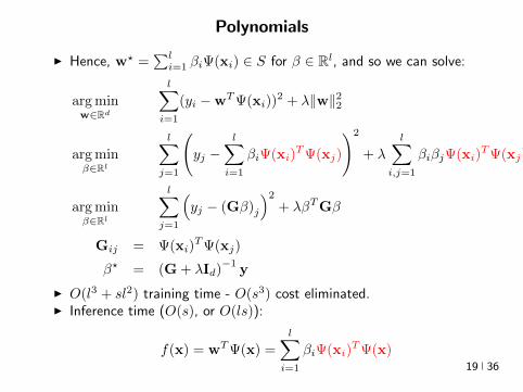
Polynomials
I Hence w =sumli=1 βiΨ(xi) isin S for β isin Rl and so we can solve
arg minwisinRd
lsumi=1
(yi minuswTΨ(xi))2 + λw22
arg minβisinRl
lsumj=1
(yj minus
lsumi=1
βiΨ(xi)TΨ(xj)
)2
+ λ
lsumij=1
βiβjΨ(xi)TΨ(xj)
arg minβisinRl
lsumj=1
(yj minus (Gβ)j
)2+ λβTGβ
Gij = Ψ(xi)TΨ(xj)
β = (G + λId)minus1
y
I O(l3 + sl2) training time - O(s3) cost eliminatedI Inference time (O(s) or O(ls))
f(x) = wTΨ(x) =
lsumi=1
βiΨ(xi)TΨ(x)
19 36
Polynomials
I Multinomial Theorem
(z1 + z2 + + zn)d =sum
α|α|=d
(d
α
)zα
I Implicit computation of inner products
Ψ(x)TΨ(xprime) =
ssumi=1
(d
α
)xαxprime
α=
ssumi=1
(d
α
)xα11 xαnn x
primeα11 x
primeαnn
=
ssumi=1
(d
α
)(x1x
prime1)α1(x2x
prime2)α2 (xnx
primen)αn
= (x1xprime1 + xnx
primen)d
= (xTxprime)d
I O(l3 + l2n) training and O(ln) predicting speedI Complexity coming from s has been completely eliminated ()
[Kernel Trick]
20 36
Polynomials Algorithm
I Algorithm
ndash Start with k X times X 7rarr R k(xxprime) = (xTxprime + 1)d
ndash Construct Gram matrix Gij = k(xixj) on the training samplesndash Solve β = (G + λId)minus1 yndash Return f(x) =
sumli=1 βik(xix)
I f is the optimal degree-d polynomial solving the learning problemin complexity independent of d
I What other forms of k correspond to linear learning inhigh-dimensional nonlinear embeddings of the data
21 36
Symmetric positive semi-definite functions
I Definition A function k X times X 7rarr R is psd if for any finitecollection of points x1 xl the l times l Gram matrix
Gij = k(xixj)
is positive semi-definite ie for any vector β isin Rl
βTGβ =sumij
βiβjk(xixj) ge 0
I Theorem[Mercer] If k is symmetric psd X is compact subset ofRn then it admits an eigenfunction decomposition
k(xxprime) =
Nsumi=1
λiφj(x)φj(xprime) = 〈Ψ(x)Ψ(xprime)〉l2
Ψ(x) = [ radicλjφ(x) ]T (3)
I Feature map associated with a kernel is not uniqueI Functional generalization of positive semi-definite matrices
22 36
Kernels
I Lineark(xxprime) = xTxprime
I Polynomialk(xxprime) = (xTxprime + 1)d
I Gaussian s =infin Universal
k(xxprime) = eminusxminusxprime2
2σ2
I Conic combinations
k(xxprime) = α1k1(xxprime) + α2k2(xxprime)
I Elementwise products
k(xxprime) = k1(xxprime)k2(xxprime)
I Kernels on discrete sets strings graphs sequences shapes
23 36
Gaussian Kernel is Positive Definite
I Exponential
eβxTxprime = 1 + βxTxprime +
β2
2(xTy)2 +
β3
3(xTy)3 +
I For any function f Rn 7rarr R psd function k the following kernelis psd
kprime(xxprime) = f(x) (k(xxprime)) f(xprime)
Proofsumij
βiβjkprime(xixj) =
sumij
βiβjf(xi)k(xixj)f(xj) =sumij
βprimeiβprimejk(xixj) ge 0
I Gaussian Kernel
k(xxprime) = eminusxminusxprime22
2σ2
= eminusx222σ2
(e
2xT xprime2σ2
)eminusxprime222σ2 (4)
24 36
The Mathematical Naturalness of Kernel Methods
I Data X isin Rd Models isin H X 7rarr R
I Geometry in H inner product 〈middot middot〉H norm middot H (Hilbert Spaces)I Theorem All nice Hilbert spaces are generated by a symmetric
positive definite function (the kernel) k(xxprime) on X times XI if f g isin H close ie f minus gH small then f(x) g(x) close forallx isin X I Reproducing Kernel Hilbert Spaces (RKHSs) Hilbert space H
that admit a reproducing kernel ie a function k(xxprime) satisfying
(i) forallx isin X k(middotx) isin H(ii) 〈f k(middotx)〉H = f(x)
I Reproducing kernels are symmetric psdsumij
βiβjk(xixj) = 〈sumi
βik(middotxi)sumi
βik(middotxi)〉H
= sumi
βik(middotxi)2H ge 0 (5)
I (Moore-Aronsjan 1950) Symmetric psd functions arereproducing kernels for some (unique) RKHS Hk
25 36
The Mathematical Naturalness of Kernel Methods
I Data X isin Rd Models isin H X 7rarr RI Geometry in H inner product 〈middot middot〉H norm middot H (Hilbert Spaces)
I Theorem All nice Hilbert spaces are generated by a symmetricpositive definite function (the kernel) k(xxprime) on X times X
I if f g isin H close ie f minus gH small then f(x) g(x) close forallx isin X I Reproducing Kernel Hilbert Spaces (RKHSs) Hilbert space H
that admit a reproducing kernel ie a function k(xxprime) satisfying
(i) forallx isin X k(middotx) isin H(ii) 〈f k(middotx)〉H = f(x)
I Reproducing kernels are symmetric psdsumij
βiβjk(xixj) = 〈sumi
βik(middotxi)sumi
βik(middotxi)〉H
= sumi
βik(middotxi)2H ge 0 (5)
I (Moore-Aronsjan 1950) Symmetric psd functions arereproducing kernels for some (unique) RKHS Hk
25 36
The Mathematical Naturalness of Kernel Methods
I Data X isin Rd Models isin H X 7rarr RI Geometry in H inner product 〈middot middot〉H norm middot H (Hilbert Spaces)I Theorem All nice Hilbert spaces are generated by a symmetric
positive definite function (the kernel) k(xxprime) on X times XI if f g isin H close ie f minus gH small then f(x) g(x) close forallx isin X
I Reproducing Kernel Hilbert Spaces (RKHSs) Hilbert space Hthat admit a reproducing kernel ie a function k(xxprime) satisfying
(i) forallx isin X k(middotx) isin H(ii) 〈f k(middotx)〉H = f(x)
I Reproducing kernels are symmetric psdsumij
βiβjk(xixj) = 〈sumi
βik(middotxi)sumi
βik(middotxi)〉H
= sumi
βik(middotxi)2H ge 0 (5)
I (Moore-Aronsjan 1950) Symmetric psd functions arereproducing kernels for some (unique) RKHS Hk
25 36
The Mathematical Naturalness of Kernel Methods
I Data X isin Rd Models isin H X 7rarr RI Geometry in H inner product 〈middot middot〉H norm middot H (Hilbert Spaces)I Theorem All nice Hilbert spaces are generated by a symmetric
positive definite function (the kernel) k(xxprime) on X times XI if f g isin H close ie f minus gH small then f(x) g(x) close forallx isin X I Reproducing Kernel Hilbert Spaces (RKHSs) Hilbert space H
that admit a reproducing kernel ie a function k(xxprime) satisfying
(i) forallx isin X k(middotx) isin H(ii) 〈f k(middotx)〉H = f(x)
I Reproducing kernels are symmetric psdsumij
βiβjk(xixj) = 〈sumi
βik(middotxi)sumi
βik(middotxi)〉H
= sumi
βik(middotxi)2H ge 0 (5)
I (Moore-Aronsjan 1950) Symmetric psd functions arereproducing kernels for some (unique) RKHS Hk
25 36
The Mathematical Naturalness of Kernel Methods
I Data X isin Rd Models isin H X 7rarr RI Geometry in H inner product 〈middot middot〉H norm middot H (Hilbert Spaces)I Theorem All nice Hilbert spaces are generated by a symmetric
positive definite function (the kernel) k(xxprime) on X times XI if f g isin H close ie f minus gH small then f(x) g(x) close forallx isin X I Reproducing Kernel Hilbert Spaces (RKHSs) Hilbert space H
that admit a reproducing kernel ie a function k(xxprime) satisfying
(i) forallx isin X k(middotx) isin H(ii) 〈f k(middotx)〉H = f(x)
I Reproducing kernels are symmetric psdsumij
βiβjk(xixj) = 〈sumi
βik(middotxi)sumi
βik(middotxi)〉H
= sumi
βik(middotxi)2H ge 0 (5)
I (Moore-Aronsjan 1950) Symmetric psd functions arereproducing kernels for some (unique) RKHS Hk 25 36
Kernel Methods Summary
I Symm pos def function k(x z) on input domain X sub Rd
I k hArr rich Reproducing Kernel Hilbert Space (RKHS) Hk ofreal-valued functions with inner product 〈middot middot〉k and norm middot k
I Regularized Risk Minimization hArr Linear models in an implicithigh-dimensional (often infinite-dimensional) feature space
f = arg minfisinHk
1
n
nsumi=1
V (yi f(xi)) + λf2Hk xi isin Rd
I Representer Theorem f(x) =sumni=1 αik(xxi)
26 36
Shallow and Deep Function Spaces
I What does it mean to understand a function space
ndash Linear f(x) = wTxw isin Rd
ndash Polynomial f(x) = wT Ψ(x)w isin Rs
ndash RKHS balls f isin Hk fk lt γ [like vM le 1]
I Shallow nets f(x) = wTσ(Wx) (w isin RdW isin Rs)ndash For srarrinfin W sim p σ(u) = eminusiu approximates Gaussian kernel
methodsndash Theorem [Bochner 1937] One-to-one correspondence between k
and a density p such that
k(x z) = ψ(xminus z) =
intRdeminusi(xminusz)Twp(w)dw asymp 1
s
ssumj=1
eminusi(xminusz)Twj
Gaussian kernel k(x z) = eminusxminusz22
2σ2 lArrrArr p = N (0 σminus2Id)ndash Similar integral approx relates ReLU to the arc-cosine kernelndash Optimization versus Randomization
27 36
Shallow and Deep Function Spaces
I What does it mean to understand a function space
ndash Linear f(x) = wTxw isin Rd
ndash Polynomial f(x) = wT Ψ(x)w isin Rs
ndash RKHS balls f isin Hk fk lt γ [like vM le 1]
I Shallow nets f(x) = wTσ(Wx) (w isin RdW isin Rs)ndash For srarrinfin W sim p σ(u) = eminusiu approximates Gaussian kernel
methodsndash Theorem [Bochner 1937] One-to-one correspondence between k
and a density p such that
k(x z) = ψ(xminus z) =
intRdeminusi(xminusz)Twp(w)dw asymp 1
s
ssumj=1
eminusi(xminusz)Twj
Gaussian kernel k(x z) = eminusxminusz22
2σ2 lArrrArr p = N (0 σminus2Id)ndash Similar integral approx relates ReLU to the arc-cosine kernelndash Optimization versus Randomization
27 36
Shallow and Deep Function Spaces
I What does it mean to understand a function space
ndash Linear f(x) = wTxw isin Rd
ndash Polynomial f(x) = wT Ψ(x)w isin Rs
ndash RKHS balls f isin Hk fk lt γ [like vM le 1]
I Shallow nets f(x) = wTσ(Wx) (w isin RdW isin Rs)ndash For srarrinfin W sim p σ(u) = eminusiu approximates Gaussian kernel
methodsndash Theorem [Bochner 1937] One-to-one correspondence between k
and a density p such that
k(x z) = ψ(xminus z) =
intRdeminusi(xminusz)Twp(w)dw asymp 1
s
ssumj=1
eminusi(xminusz)Twj
Gaussian kernel k(x z) = eminusxminusz22
2σ2 lArrrArr p = N (0 σminus2Id)ndash Similar integral approx relates ReLU to the arc-cosine kernelndash Optimization versus Randomization
27 36
Shallow and Deep Function Spaces
I What does it mean to understand a function space
ndash Linear f(x) = wTxw isin Rd
ndash Polynomial f(x) = wT Ψ(x)w isin Rs
ndash RKHS balls f isin Hk fk lt γ [like vM le 1]
I Shallow nets f(x) = wTσ(Wx) (w isin RdW isin Rs)
ndash For srarrinfin W sim p σ(u) = eminusiu approximates Gaussian kernelmethods
ndash Theorem [Bochner 1937] One-to-one correspondence between kand a density p such that
k(x z) = ψ(xminus z) =
intRdeminusi(xminusz)Twp(w)dw asymp 1
s
ssumj=1
eminusi(xminusz)Twj
Gaussian kernel k(x z) = eminusxminusz22
2σ2 lArrrArr p = N (0 σminus2Id)ndash Similar integral approx relates ReLU to the arc-cosine kernelndash Optimization versus Randomization
27 36
Shallow and Deep Function Spaces
I What does it mean to understand a function space
ndash Linear f(x) = wTxw isin Rd
ndash Polynomial f(x) = wT Ψ(x)w isin Rs
ndash RKHS balls f isin Hk fk lt γ [like vM le 1]
I Shallow nets f(x) = wTσ(Wx) (w isin RdW isin Rs)ndash For srarrinfin W sim p σ(u) = eminusiu approximates Gaussian kernel
methodsndash Theorem [Bochner 1937] One-to-one correspondence between k
and a density p such that
k(x z) = ψ(xminus z) =
intRdeminusi(xminusz)Twp(w)dw asymp 1
s
ssumj=1
eminusi(xminusz)Twj
Gaussian kernel k(x z) = eminusxminusz22
2σ2 lArrrArr p = N (0 σminus2Id)ndash Similar integral approx relates ReLU to the arc-cosine kernelndash Optimization versus Randomization
27 36
Expressivity of Deep Nets Linear Regions
I The ReLU map f(x) = max(Wx 0)W isin Rwtimesn is piecewise linear
I A piece is a connected region (a convex polytope) of Rd with sharedsparsity pattern in activations
I (Zaslavsky 1975) Number of linear regions formed by an arrangement of
s hyperplanes in d-dimensions in general position issumd
i=0
(si
)I Composition of ReLU maps is also piecewise linear
I (Raghu et al 2017 Pascano et al 2014 Montufar 2014) Number oflinear regions grows as O(wnd) for a composition of d ReLU maps(nrarr brarr brarr b rarr b) each of width w
I (Safran and Shamir 2017)
ndash 1[x le 1] x isin Rd ε-accurate 3-layer network with O(dε) neurons but cannot be approximated with
accuracy higher than O(1d4) using 2-layer networks unless width is exponential in d
28 36
Expressivity of Deep Nets Linear Regions
I The ReLU map f(x) = max(Wx 0)W isin Rwtimesn is piecewise linear
I A piece is a connected region (a convex polytope) of Rd with sharedsparsity pattern in activations
I (Zaslavsky 1975) Number of linear regions formed by an arrangement of
s hyperplanes in d-dimensions in general position issumd
i=0
(si
)I Composition of ReLU maps is also piecewise linear
I (Raghu et al 2017 Pascano et al 2014 Montufar 2014) Number oflinear regions grows as O(wnd) for a composition of d ReLU maps(nrarr brarr brarr b rarr b) each of width w
I (Safran and Shamir 2017)
ndash 1[x le 1] x isin Rd ε-accurate 3-layer network with O(dε) neurons but cannot be approximated with
accuracy higher than O(1d4) using 2-layer networks unless width is exponential in d
28 36
Expressivity of Deep Nets Linear Regions
I The ReLU map f(x) = max(Wx 0)W isin Rwtimesn is piecewise linear
I A piece is a connected region (a convex polytope) of Rd with sharedsparsity pattern in activations
I (Zaslavsky 1975) Number of linear regions formed by an arrangement of
s hyperplanes in d-dimensions in general position issumd
i=0
(si
)
I Composition of ReLU maps is also piecewise linear
I (Raghu et al 2017 Pascano et al 2014 Montufar 2014) Number oflinear regions grows as O(wnd) for a composition of d ReLU maps(nrarr brarr brarr b rarr b) each of width w
I (Safran and Shamir 2017)
ndash 1[x le 1] x isin Rd ε-accurate 3-layer network with O(dε) neurons but cannot be approximated with
accuracy higher than O(1d4) using 2-layer networks unless width is exponential in d
28 36
Expressivity of Deep Nets Linear Regions
I The ReLU map f(x) = max(Wx 0)W isin Rwtimesn is piecewise linear
I A piece is a connected region (a convex polytope) of Rd with sharedsparsity pattern in activations
I (Zaslavsky 1975) Number of linear regions formed by an arrangement of
s hyperplanes in d-dimensions in general position issumd
i=0
(si
)I Composition of ReLU maps is also piecewise linear
I (Raghu et al 2017 Pascano et al 2014 Montufar 2014) Number oflinear regions grows as O(wnd) for a composition of d ReLU maps(nrarr brarr brarr b rarr b) each of width w
I (Safran and Shamir 2017)
ndash 1[x le 1] x isin Rd ε-accurate 3-layer network with O(dε) neurons but cannot be approximated with
accuracy higher than O(1d4) using 2-layer networks unless width is exponential in d28 36
Expressivity of Deep Nets Trajectory Length
I (Raghu et al 2017) Trajectory Length (ldquogeneralized operator normrdquo)How much is a curve in the input space stretched by a layer in thenetwork
29 36
Expressivity of Deep Nets Trajectory Length
I (Raghu et al 2017) Trajectory Length (ldquogeneralized operator normrdquo)How much is a curve in the input space stretched by a layer in thenetwork
29 36
Expressivity and Generalization
I Expressiveness equiv capacity to fit random noise =rArr susceptibility tooverfitting (VC dimension Rademacher Complexity)
I Zhang et al 2017 Famous CNNs easily fit random labels
ndash Over-parameterized (n=12M psim 60M) but structuredndash Domain-knowledge baked in does not constraint expressiveness
I CNNs tend to generalize even without regularization (explicit and implicit)
I For linear regression SGD returns minimum norm solution
30 36
Expressivity and Generalization
I Expressiveness equiv capacity to fit random noise =rArr susceptibility tooverfitting (VC dimension Rademacher Complexity)
I Zhang et al 2017 Famous CNNs easily fit random labels
ndash Over-parameterized (n=12M psim 60M) but structuredndash Domain-knowledge baked in does not constraint expressiveness
I CNNs tend to generalize even without regularization (explicit and implicit)
I For linear regression SGD returns minimum norm solution
30 36
Expressivity and Generalization
I Expressiveness equiv capacity to fit random noise =rArr susceptibility tooverfitting (VC dimension Rademacher Complexity)
I Zhang et al 2017 Famous CNNs easily fit random labels
ndash Over-parameterized (n=12M psim 60M) but structuredndash Domain-knowledge baked in does not constraint expressiveness
I CNNs tend to generalize even without regularization (explicit and implicit)
I For linear regression SGD returns minimum norm solution
30 36
Optimization Landscape Symmetry and Saddle Points
I Folklore lots of equivalent good local minI Classification of critical points based on Hessian spectrumI Permutation and Scaling symmetries
I Thm [Lee et al 2016 Anadkumar Ge] For the short-step gradientmethod the basin of attraction of strict saddle points (atleast onenegative eigenvalue) has measure zero
31 36
Optimization Landscape Symmetry and Saddle Points
I Folklore lots of equivalent good local minI Classification of critical points based on Hessian spectrumI Permutation and Scaling symmetries
I Thm [Lee et al 2016 Anadkumar Ge] For the short-step gradientmethod the basin of attraction of strict saddle points (atleast onenegative eigenvalue) has measure zero
31 36
Optimization Landscape Symmetry and Saddle Points
I Folklore lots of equivalent good local minI Classification of critical points based on Hessian spectrumI Permutation and Scaling symmetries
I Thm [Lee et al 2016 Anadkumar Ge] For the short-step gradientmethod the basin of attraction of strict saddle points (atleast onenegative eigenvalue) has measure zero
31 36
Optimization Landscape Sharp Minima and Stability
Keskar et al 2017 On large-batch training for DL Generalization Gap and Sharp Minima
32 36
Deep Learning Computational Graphs TensorFlow
tensorfloworg
I Tensors-in Tensors-out
I Evergrowing list of Tensor-Ops (PythonC++)
f(xw)
[partf
partx
]T v
[partf
partw
]T v
I Automatic Differentiation Reverse mode
partxL
partxi=sumirarrj
partxL
partxj
partxj
partxi
33 36
Computational Graphs and TensorFlow
tensorfloworg
I SGD with minibatches
wk+1 = wk minus ηlsumi=1
partli
partw
∣∣∣wt
I Model Parallelism Assign independent paths tothreads GPUs
I Data Parallelism create Graph replicas on differentmachines
I Mobile TensorFlow
34 36
Computational Graphs and TensorFlow
tensorfloworg
35 36
Computational Graphs and TensorFlow
tensorfloworg
35 36
Computational Graphs and TensorFlow
tensorfloworg
35 36
Challenges and Opportunities
I Lots of fascinating unsolved problems
I Can you win Imagenet with Convex optimization
I Tools from polynomial optimization (global optimization deep-RL)
I Supervised to Semi-supervised to Unsupervised Learning
I Compact efficient real-time models (eliminateover-parametrization) for new form factors
I Exciting emerging world of Robotics Wearable ComputersIntelligent home devices Personal digital assistants
Google Internship Program
36 36
- anm0
- fdrm0
- fdrm5
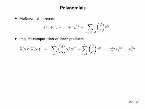
Polynomials
I Multinomial Theorem
(z1 + z2 + + zn)d =sum
α|α|=d
(d
α
)zα
I Implicit computation of inner products
Ψ(x)TΨ(xprime) =
ssumi=1
(d
α
)xαxprime
α=
ssumi=1
(d
α
)xα11 xαnn x
primeα11 x
primeαnn
=
ssumi=1
(d
α
)(x1x
prime1)α1(x2x
prime2)α2 (xnx
primen)αn
= (x1xprime1 + xnx
primen)d
= (xTxprime)d
I O(l3 + l2n) training and O(ln) predicting speedI Complexity coming from s has been completely eliminated ()
[Kernel Trick]
20 36
Polynomials Algorithm
I Algorithm
ndash Start with k X times X 7rarr R k(xxprime) = (xTxprime + 1)d
ndash Construct Gram matrix Gij = k(xixj) on the training samplesndash Solve β = (G + λId)minus1 yndash Return f(x) =
sumli=1 βik(xix)
I f is the optimal degree-d polynomial solving the learning problemin complexity independent of d
I What other forms of k correspond to linear learning inhigh-dimensional nonlinear embeddings of the data
21 36
Symmetric positive semi-definite functions
I Definition A function k X times X 7rarr R is psd if for any finitecollection of points x1 xl the l times l Gram matrix
Gij = k(xixj)
is positive semi-definite ie for any vector β isin Rl
βTGβ =sumij
βiβjk(xixj) ge 0
I Theorem[Mercer] If k is symmetric psd X is compact subset ofRn then it admits an eigenfunction decomposition
k(xxprime) =
Nsumi=1
λiφj(x)φj(xprime) = 〈Ψ(x)Ψ(xprime)〉l2
Ψ(x) = [ radicλjφ(x) ]T (3)
I Feature map associated with a kernel is not uniqueI Functional generalization of positive semi-definite matrices
22 36
Kernels
I Lineark(xxprime) = xTxprime
I Polynomialk(xxprime) = (xTxprime + 1)d
I Gaussian s =infin Universal
k(xxprime) = eminusxminusxprime2
2σ2
I Conic combinations
k(xxprime) = α1k1(xxprime) + α2k2(xxprime)
I Elementwise products
k(xxprime) = k1(xxprime)k2(xxprime)
I Kernels on discrete sets strings graphs sequences shapes
23 36
Gaussian Kernel is Positive Definite
I Exponential
eβxTxprime = 1 + βxTxprime +
β2
2(xTy)2 +
β3
3(xTy)3 +
I For any function f Rn 7rarr R psd function k the following kernelis psd
kprime(xxprime) = f(x) (k(xxprime)) f(xprime)
Proofsumij
βiβjkprime(xixj) =
sumij
βiβjf(xi)k(xixj)f(xj) =sumij
βprimeiβprimejk(xixj) ge 0
I Gaussian Kernel
k(xxprime) = eminusxminusxprime22
2σ2
= eminusx222σ2
(e
2xT xprime2σ2
)eminusxprime222σ2 (4)
24 36
The Mathematical Naturalness of Kernel Methods
I Data X isin Rd Models isin H X 7rarr R
I Geometry in H inner product 〈middot middot〉H norm middot H (Hilbert Spaces)I Theorem All nice Hilbert spaces are generated by a symmetric
positive definite function (the kernel) k(xxprime) on X times XI if f g isin H close ie f minus gH small then f(x) g(x) close forallx isin X I Reproducing Kernel Hilbert Spaces (RKHSs) Hilbert space H
that admit a reproducing kernel ie a function k(xxprime) satisfying
(i) forallx isin X k(middotx) isin H(ii) 〈f k(middotx)〉H = f(x)
I Reproducing kernels are symmetric psdsumij
βiβjk(xixj) = 〈sumi
βik(middotxi)sumi
βik(middotxi)〉H
= sumi
βik(middotxi)2H ge 0 (5)
I (Moore-Aronsjan 1950) Symmetric psd functions arereproducing kernels for some (unique) RKHS Hk
25 36
The Mathematical Naturalness of Kernel Methods
I Data X isin Rd Models isin H X 7rarr RI Geometry in H inner product 〈middot middot〉H norm middot H (Hilbert Spaces)
I Theorem All nice Hilbert spaces are generated by a symmetricpositive definite function (the kernel) k(xxprime) on X times X
I if f g isin H close ie f minus gH small then f(x) g(x) close forallx isin X I Reproducing Kernel Hilbert Spaces (RKHSs) Hilbert space H
that admit a reproducing kernel ie a function k(xxprime) satisfying
(i) forallx isin X k(middotx) isin H(ii) 〈f k(middotx)〉H = f(x)
I Reproducing kernels are symmetric psdsumij
βiβjk(xixj) = 〈sumi
βik(middotxi)sumi
βik(middotxi)〉H
= sumi
βik(middotxi)2H ge 0 (5)
I (Moore-Aronsjan 1950) Symmetric psd functions arereproducing kernels for some (unique) RKHS Hk
25 36
The Mathematical Naturalness of Kernel Methods
I Data X isin Rd Models isin H X 7rarr RI Geometry in H inner product 〈middot middot〉H norm middot H (Hilbert Spaces)I Theorem All nice Hilbert spaces are generated by a symmetric
positive definite function (the kernel) k(xxprime) on X times XI if f g isin H close ie f minus gH small then f(x) g(x) close forallx isin X
I Reproducing Kernel Hilbert Spaces (RKHSs) Hilbert space Hthat admit a reproducing kernel ie a function k(xxprime) satisfying
(i) forallx isin X k(middotx) isin H(ii) 〈f k(middotx)〉H = f(x)
I Reproducing kernels are symmetric psdsumij
βiβjk(xixj) = 〈sumi
βik(middotxi)sumi
βik(middotxi)〉H
= sumi
βik(middotxi)2H ge 0 (5)
I (Moore-Aronsjan 1950) Symmetric psd functions arereproducing kernels for some (unique) RKHS Hk
25 36
The Mathematical Naturalness of Kernel Methods
I Data X isin Rd Models isin H X 7rarr RI Geometry in H inner product 〈middot middot〉H norm middot H (Hilbert Spaces)I Theorem All nice Hilbert spaces are generated by a symmetric
positive definite function (the kernel) k(xxprime) on X times XI if f g isin H close ie f minus gH small then f(x) g(x) close forallx isin X I Reproducing Kernel Hilbert Spaces (RKHSs) Hilbert space H
that admit a reproducing kernel ie a function k(xxprime) satisfying
(i) forallx isin X k(middotx) isin H(ii) 〈f k(middotx)〉H = f(x)
I Reproducing kernels are symmetric psdsumij
βiβjk(xixj) = 〈sumi
βik(middotxi)sumi
βik(middotxi)〉H
= sumi
βik(middotxi)2H ge 0 (5)
I (Moore-Aronsjan 1950) Symmetric psd functions arereproducing kernels for some (unique) RKHS Hk
25 36
The Mathematical Naturalness of Kernel Methods
I Data X isin Rd Models isin H X 7rarr RI Geometry in H inner product 〈middot middot〉H norm middot H (Hilbert Spaces)I Theorem All nice Hilbert spaces are generated by a symmetric
positive definite function (the kernel) k(xxprime) on X times XI if f g isin H close ie f minus gH small then f(x) g(x) close forallx isin X I Reproducing Kernel Hilbert Spaces (RKHSs) Hilbert space H
that admit a reproducing kernel ie a function k(xxprime) satisfying
(i) forallx isin X k(middotx) isin H(ii) 〈f k(middotx)〉H = f(x)
I Reproducing kernels are symmetric psdsumij
βiβjk(xixj) = 〈sumi
βik(middotxi)sumi
βik(middotxi)〉H
= sumi
βik(middotxi)2H ge 0 (5)
I (Moore-Aronsjan 1950) Symmetric psd functions arereproducing kernels for some (unique) RKHS Hk 25 36
Kernel Methods Summary
I Symm pos def function k(x z) on input domain X sub Rd
I k hArr rich Reproducing Kernel Hilbert Space (RKHS) Hk ofreal-valued functions with inner product 〈middot middot〉k and norm middot k
I Regularized Risk Minimization hArr Linear models in an implicithigh-dimensional (often infinite-dimensional) feature space
f = arg minfisinHk
1
n
nsumi=1
V (yi f(xi)) + λf2Hk xi isin Rd
I Representer Theorem f(x) =sumni=1 αik(xxi)
26 36
Shallow and Deep Function Spaces
I What does it mean to understand a function space
ndash Linear f(x) = wTxw isin Rd
ndash Polynomial f(x) = wT Ψ(x)w isin Rs
ndash RKHS balls f isin Hk fk lt γ [like vM le 1]
I Shallow nets f(x) = wTσ(Wx) (w isin RdW isin Rs)ndash For srarrinfin W sim p σ(u) = eminusiu approximates Gaussian kernel
methodsndash Theorem [Bochner 1937] One-to-one correspondence between k
and a density p such that
k(x z) = ψ(xminus z) =
intRdeminusi(xminusz)Twp(w)dw asymp 1
s
ssumj=1
eminusi(xminusz)Twj
Gaussian kernel k(x z) = eminusxminusz22
2σ2 lArrrArr p = N (0 σminus2Id)ndash Similar integral approx relates ReLU to the arc-cosine kernelndash Optimization versus Randomization
27 36
Shallow and Deep Function Spaces
I What does it mean to understand a function space
ndash Linear f(x) = wTxw isin Rd
ndash Polynomial f(x) = wT Ψ(x)w isin Rs
ndash RKHS balls f isin Hk fk lt γ [like vM le 1]
I Shallow nets f(x) = wTσ(Wx) (w isin RdW isin Rs)ndash For srarrinfin W sim p σ(u) = eminusiu approximates Gaussian kernel
methodsndash Theorem [Bochner 1937] One-to-one correspondence between k
and a density p such that
k(x z) = ψ(xminus z) =
intRdeminusi(xminusz)Twp(w)dw asymp 1
s
ssumj=1
eminusi(xminusz)Twj
Gaussian kernel k(x z) = eminusxminusz22
2σ2 lArrrArr p = N (0 σminus2Id)ndash Similar integral approx relates ReLU to the arc-cosine kernelndash Optimization versus Randomization
27 36
Shallow and Deep Function Spaces
I What does it mean to understand a function space
ndash Linear f(x) = wTxw isin Rd
ndash Polynomial f(x) = wT Ψ(x)w isin Rs
ndash RKHS balls f isin Hk fk lt γ [like vM le 1]
I Shallow nets f(x) = wTσ(Wx) (w isin RdW isin Rs)ndash For srarrinfin W sim p σ(u) = eminusiu approximates Gaussian kernel
methodsndash Theorem [Bochner 1937] One-to-one correspondence between k
and a density p such that
k(x z) = ψ(xminus z) =
intRdeminusi(xminusz)Twp(w)dw asymp 1
s
ssumj=1
eminusi(xminusz)Twj
Gaussian kernel k(x z) = eminusxminusz22
2σ2 lArrrArr p = N (0 σminus2Id)ndash Similar integral approx relates ReLU to the arc-cosine kernelndash Optimization versus Randomization
27 36
Shallow and Deep Function Spaces
I What does it mean to understand a function space
ndash Linear f(x) = wTxw isin Rd
ndash Polynomial f(x) = wT Ψ(x)w isin Rs
ndash RKHS balls f isin Hk fk lt γ [like vM le 1]
I Shallow nets f(x) = wTσ(Wx) (w isin RdW isin Rs)
ndash For srarrinfin W sim p σ(u) = eminusiu approximates Gaussian kernelmethods
ndash Theorem [Bochner 1937] One-to-one correspondence between kand a density p such that
k(x z) = ψ(xminus z) =
intRdeminusi(xminusz)Twp(w)dw asymp 1
s
ssumj=1
eminusi(xminusz)Twj
Gaussian kernel k(x z) = eminusxminusz22
2σ2 lArrrArr p = N (0 σminus2Id)ndash Similar integral approx relates ReLU to the arc-cosine kernelndash Optimization versus Randomization
27 36
Shallow and Deep Function Spaces
I What does it mean to understand a function space
ndash Linear f(x) = wTxw isin Rd
ndash Polynomial f(x) = wT Ψ(x)w isin Rs
ndash RKHS balls f isin Hk fk lt γ [like vM le 1]
I Shallow nets f(x) = wTσ(Wx) (w isin RdW isin Rs)ndash For srarrinfin W sim p σ(u) = eminusiu approximates Gaussian kernel
methodsndash Theorem [Bochner 1937] One-to-one correspondence between k
and a density p such that
k(x z) = ψ(xminus z) =
intRdeminusi(xminusz)Twp(w)dw asymp 1
s
ssumj=1
eminusi(xminusz)Twj
Gaussian kernel k(x z) = eminusxminusz22
2σ2 lArrrArr p = N (0 σminus2Id)ndash Similar integral approx relates ReLU to the arc-cosine kernelndash Optimization versus Randomization
27 36
Expressivity of Deep Nets Linear Regions
I The ReLU map f(x) = max(Wx 0)W isin Rwtimesn is piecewise linear
I A piece is a connected region (a convex polytope) of Rd with sharedsparsity pattern in activations
I (Zaslavsky 1975) Number of linear regions formed by an arrangement of
s hyperplanes in d-dimensions in general position issumd
i=0
(si
)I Composition of ReLU maps is also piecewise linear
I (Raghu et al 2017 Pascano et al 2014 Montufar 2014) Number oflinear regions grows as O(wnd) for a composition of d ReLU maps(nrarr brarr brarr b rarr b) each of width w
I (Safran and Shamir 2017)
ndash 1[x le 1] x isin Rd ε-accurate 3-layer network with O(dε) neurons but cannot be approximated with
accuracy higher than O(1d4) using 2-layer networks unless width is exponential in d
28 36
Expressivity of Deep Nets Linear Regions
I The ReLU map f(x) = max(Wx 0)W isin Rwtimesn is piecewise linear
I A piece is a connected region (a convex polytope) of Rd with sharedsparsity pattern in activations
I (Zaslavsky 1975) Number of linear regions formed by an arrangement of
s hyperplanes in d-dimensions in general position issumd
i=0
(si
)I Composition of ReLU maps is also piecewise linear
I (Raghu et al 2017 Pascano et al 2014 Montufar 2014) Number oflinear regions grows as O(wnd) for a composition of d ReLU maps(nrarr brarr brarr b rarr b) each of width w
I (Safran and Shamir 2017)
ndash 1[x le 1] x isin Rd ε-accurate 3-layer network with O(dε) neurons but cannot be approximated with
accuracy higher than O(1d4) using 2-layer networks unless width is exponential in d
28 36
Expressivity of Deep Nets Linear Regions
I The ReLU map f(x) = max(Wx 0)W isin Rwtimesn is piecewise linear
I A piece is a connected region (a convex polytope) of Rd with sharedsparsity pattern in activations
I (Zaslavsky 1975) Number of linear regions formed by an arrangement of
s hyperplanes in d-dimensions in general position issumd
i=0
(si
)
I Composition of ReLU maps is also piecewise linear
I (Raghu et al 2017 Pascano et al 2014 Montufar 2014) Number oflinear regions grows as O(wnd) for a composition of d ReLU maps(nrarr brarr brarr b rarr b) each of width w
I (Safran and Shamir 2017)
ndash 1[x le 1] x isin Rd ε-accurate 3-layer network with O(dε) neurons but cannot be approximated with
accuracy higher than O(1d4) using 2-layer networks unless width is exponential in d
28 36
Expressivity of Deep Nets Linear Regions
I The ReLU map f(x) = max(Wx 0)W isin Rwtimesn is piecewise linear
I A piece is a connected region (a convex polytope) of Rd with sharedsparsity pattern in activations
I (Zaslavsky 1975) Number of linear regions formed by an arrangement of
s hyperplanes in d-dimensions in general position issumd
i=0
(si
)I Composition of ReLU maps is also piecewise linear
I (Raghu et al 2017 Pascano et al 2014 Montufar 2014) Number oflinear regions grows as O(wnd) for a composition of d ReLU maps(nrarr brarr brarr b rarr b) each of width w
I (Safran and Shamir 2017)
ndash 1[x le 1] x isin Rd ε-accurate 3-layer network with O(dε) neurons but cannot be approximated with
accuracy higher than O(1d4) using 2-layer networks unless width is exponential in d28 36
Expressivity of Deep Nets Trajectory Length
I (Raghu et al 2017) Trajectory Length (ldquogeneralized operator normrdquo)How much is a curve in the input space stretched by a layer in thenetwork
29 36
Expressivity of Deep Nets Trajectory Length
I (Raghu et al 2017) Trajectory Length (ldquogeneralized operator normrdquo)How much is a curve in the input space stretched by a layer in thenetwork
29 36
Expressivity and Generalization
I Expressiveness equiv capacity to fit random noise =rArr susceptibility tooverfitting (VC dimension Rademacher Complexity)
I Zhang et al 2017 Famous CNNs easily fit random labels
ndash Over-parameterized (n=12M psim 60M) but structuredndash Domain-knowledge baked in does not constraint expressiveness
I CNNs tend to generalize even without regularization (explicit and implicit)
I For linear regression SGD returns minimum norm solution
30 36
Expressivity and Generalization
I Expressiveness equiv capacity to fit random noise =rArr susceptibility tooverfitting (VC dimension Rademacher Complexity)
I Zhang et al 2017 Famous CNNs easily fit random labels
ndash Over-parameterized (n=12M psim 60M) but structuredndash Domain-knowledge baked in does not constraint expressiveness
I CNNs tend to generalize even without regularization (explicit and implicit)
I For linear regression SGD returns minimum norm solution
30 36
Expressivity and Generalization
I Expressiveness equiv capacity to fit random noise =rArr susceptibility tooverfitting (VC dimension Rademacher Complexity)
I Zhang et al 2017 Famous CNNs easily fit random labels
ndash Over-parameterized (n=12M psim 60M) but structuredndash Domain-knowledge baked in does not constraint expressiveness
I CNNs tend to generalize even without regularization (explicit and implicit)
I For linear regression SGD returns minimum norm solution
30 36
Optimization Landscape Symmetry and Saddle Points
I Folklore lots of equivalent good local minI Classification of critical points based on Hessian spectrumI Permutation and Scaling symmetries
I Thm [Lee et al 2016 Anadkumar Ge] For the short-step gradientmethod the basin of attraction of strict saddle points (atleast onenegative eigenvalue) has measure zero
31 36
Optimization Landscape Symmetry and Saddle Points
I Folklore lots of equivalent good local minI Classification of critical points based on Hessian spectrumI Permutation and Scaling symmetries
I Thm [Lee et al 2016 Anadkumar Ge] For the short-step gradientmethod the basin of attraction of strict saddle points (atleast onenegative eigenvalue) has measure zero
31 36
Optimization Landscape Symmetry and Saddle Points
I Folklore lots of equivalent good local minI Classification of critical points based on Hessian spectrumI Permutation and Scaling symmetries
I Thm [Lee et al 2016 Anadkumar Ge] For the short-step gradientmethod the basin of attraction of strict saddle points (atleast onenegative eigenvalue) has measure zero
31 36
Optimization Landscape Sharp Minima and Stability
Keskar et al 2017 On large-batch training for DL Generalization Gap and Sharp Minima
32 36
Deep Learning Computational Graphs TensorFlow
tensorfloworg
I Tensors-in Tensors-out
I Evergrowing list of Tensor-Ops (PythonC++)
f(xw)
[partf
partx
]T v
[partf
partw
]T v
I Automatic Differentiation Reverse mode
partxL
partxi=sumirarrj
partxL
partxj
partxj
partxi
33 36
Computational Graphs and TensorFlow
tensorfloworg
I SGD with minibatches
wk+1 = wk minus ηlsumi=1
partli
partw
∣∣∣wt
I Model Parallelism Assign independent paths tothreads GPUs
I Data Parallelism create Graph replicas on differentmachines
I Mobile TensorFlow
34 36
Computational Graphs and TensorFlow
tensorfloworg
35 36
Computational Graphs and TensorFlow
tensorfloworg
35 36
Computational Graphs and TensorFlow
tensorfloworg
35 36
Challenges and Opportunities
I Lots of fascinating unsolved problems
I Can you win Imagenet with Convex optimization
I Tools from polynomial optimization (global optimization deep-RL)
I Supervised to Semi-supervised to Unsupervised Learning
I Compact efficient real-time models (eliminateover-parametrization) for new form factors
I Exciting emerging world of Robotics Wearable ComputersIntelligent home devices Personal digital assistants
Google Internship Program
36 36
- anm0
- fdrm0
- fdrm5
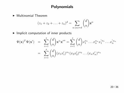
Polynomials
I Multinomial Theorem
(z1 + z2 + + zn)d =sum
α|α|=d
(d
α
)zα
I Implicit computation of inner products
Ψ(x)TΨ(xprime) =
ssumi=1
(d
α
)xαxprime
α=
ssumi=1
(d
α
)xα11 xαnn x
primeα11 x
primeαnn
=
ssumi=1
(d
α
)(x1x
prime1)α1(x2x
prime2)α2 (xnx
primen)αn
= (x1xprime1 + xnx
primen)d
= (xTxprime)d
I O(l3 + l2n) training and O(ln) predicting speedI Complexity coming from s has been completely eliminated ()
[Kernel Trick]
20 36
Polynomials
I Multinomial Theorem
(z1 + z2 + + zn)d =sum
α|α|=d
(d
α
)zα
I Implicit computation of inner products
Ψ(x)TΨ(xprime) =
ssumi=1
(d
α
)xαxprime
α=
ssumi=1
(d
α
)xα11 xαnn x
primeα11 x
primeαnn
=
ssumi=1
(d
α
)(x1x
prime1)α1(x2x
prime2)α2 (xnx
primen)αn
= (x1xprime1 + xnx
primen)d
= (xTxprime)d
I O(l3 + l2n) training and O(ln) predicting speedI Complexity coming from s has been completely eliminated ()
[Kernel Trick]
20 36
Polynomials
I Multinomial Theorem
(z1 + z2 + + zn)d =sum
α|α|=d
(d
α
)zα
I Implicit computation of inner products
Ψ(x)TΨ(xprime) =
ssumi=1
(d
α
)xαxprime
α=
ssumi=1
(d
α
)xα11 xαnn x
primeα11 x
primeαnn
=
ssumi=1
(d
α
)(x1x
prime1)α1(x2x
prime2)α2 (xnx
primen)αn
= (x1xprime1 + xnx
primen)d
= (xTxprime)d
I O(l3 + l2n) training and O(ln) predicting speedI Complexity coming from s has been completely eliminated ()
[Kernel Trick]
20 36
Polynomials
I Multinomial Theorem
(z1 + z2 + + zn)d =sum
α|α|=d
(d
α
)zα
I Implicit computation of inner products
Ψ(x)TΨ(xprime) =
ssumi=1
(d
α
)xαxprime
α=
ssumi=1
(d
α
)xα11 xαnn x
primeα11 x
primeαnn
=
ssumi=1
(d
α
)(x1x
prime1)α1(x2x
prime2)α2 (xnx
primen)αn
= (x1xprime1 + xnx
primen)d
= (xTxprime)d
I O(l3 + l2n) training and O(ln) predicting speedI Complexity coming from s has been completely eliminated ()
[Kernel Trick]
20 36
Polynomials Algorithm
I Algorithm
ndash Start with k X times X 7rarr R k(xxprime) = (xTxprime + 1)d
ndash Construct Gram matrix Gij = k(xixj) on the training samplesndash Solve β = (G + λId)minus1 yndash Return f(x) =
sumli=1 βik(xix)
I f is the optimal degree-d polynomial solving the learning problemin complexity independent of d
I What other forms of k correspond to linear learning inhigh-dimensional nonlinear embeddings of the data
21 36
Symmetric positive semi-definite functions
I Definition A function k X times X 7rarr R is psd if for any finitecollection of points x1 xl the l times l Gram matrix
Gij = k(xixj)
is positive semi-definite ie for any vector β isin Rl
βTGβ =sumij
βiβjk(xixj) ge 0
I Theorem[Mercer] If k is symmetric psd X is compact subset ofRn then it admits an eigenfunction decomposition
k(xxprime) =
Nsumi=1
λiφj(x)φj(xprime) = 〈Ψ(x)Ψ(xprime)〉l2
Ψ(x) = [ radicλjφ(x) ]T (3)
I Feature map associated with a kernel is not uniqueI Functional generalization of positive semi-definite matrices
22 36
Kernels
I Lineark(xxprime) = xTxprime
I Polynomialk(xxprime) = (xTxprime + 1)d
I Gaussian s =infin Universal
k(xxprime) = eminusxminusxprime2
2σ2
I Conic combinations
k(xxprime) = α1k1(xxprime) + α2k2(xxprime)
I Elementwise products
k(xxprime) = k1(xxprime)k2(xxprime)
I Kernels on discrete sets strings graphs sequences shapes
23 36
Gaussian Kernel is Positive Definite
I Exponential
eβxTxprime = 1 + βxTxprime +
β2
2(xTy)2 +
β3
3(xTy)3 +
I For any function f Rn 7rarr R psd function k the following kernelis psd
kprime(xxprime) = f(x) (k(xxprime)) f(xprime)
Proofsumij
βiβjkprime(xixj) =
sumij
βiβjf(xi)k(xixj)f(xj) =sumij
βprimeiβprimejk(xixj) ge 0
I Gaussian Kernel
k(xxprime) = eminusxminusxprime22
2σ2
= eminusx222σ2
(e
2xT xprime2σ2
)eminusxprime222σ2 (4)
24 36
The Mathematical Naturalness of Kernel Methods
I Data X isin Rd Models isin H X 7rarr R
I Geometry in H inner product 〈middot middot〉H norm middot H (Hilbert Spaces)I Theorem All nice Hilbert spaces are generated by a symmetric
positive definite function (the kernel) k(xxprime) on X times XI if f g isin H close ie f minus gH small then f(x) g(x) close forallx isin X I Reproducing Kernel Hilbert Spaces (RKHSs) Hilbert space H
that admit a reproducing kernel ie a function k(xxprime) satisfying
(i) forallx isin X k(middotx) isin H(ii) 〈f k(middotx)〉H = f(x)
I Reproducing kernels are symmetric psdsumij
βiβjk(xixj) = 〈sumi
βik(middotxi)sumi
βik(middotxi)〉H
= sumi
βik(middotxi)2H ge 0 (5)
I (Moore-Aronsjan 1950) Symmetric psd functions arereproducing kernels for some (unique) RKHS Hk
25 36
The Mathematical Naturalness of Kernel Methods
I Data X isin Rd Models isin H X 7rarr RI Geometry in H inner product 〈middot middot〉H norm middot H (Hilbert Spaces)
I Theorem All nice Hilbert spaces are generated by a symmetricpositive definite function (the kernel) k(xxprime) on X times X
I if f g isin H close ie f minus gH small then f(x) g(x) close forallx isin X I Reproducing Kernel Hilbert Spaces (RKHSs) Hilbert space H
that admit a reproducing kernel ie a function k(xxprime) satisfying
(i) forallx isin X k(middotx) isin H(ii) 〈f k(middotx)〉H = f(x)
I Reproducing kernels are symmetric psdsumij
βiβjk(xixj) = 〈sumi
βik(middotxi)sumi
βik(middotxi)〉H
= sumi
βik(middotxi)2H ge 0 (5)
I (Moore-Aronsjan 1950) Symmetric psd functions arereproducing kernels for some (unique) RKHS Hk
25 36
The Mathematical Naturalness of Kernel Methods
I Data X isin Rd Models isin H X 7rarr RI Geometry in H inner product 〈middot middot〉H norm middot H (Hilbert Spaces)I Theorem All nice Hilbert spaces are generated by a symmetric
positive definite function (the kernel) k(xxprime) on X times XI if f g isin H close ie f minus gH small then f(x) g(x) close forallx isin X
I Reproducing Kernel Hilbert Spaces (RKHSs) Hilbert space Hthat admit a reproducing kernel ie a function k(xxprime) satisfying
(i) forallx isin X k(middotx) isin H(ii) 〈f k(middotx)〉H = f(x)
I Reproducing kernels are symmetric psdsumij
βiβjk(xixj) = 〈sumi
βik(middotxi)sumi
βik(middotxi)〉H
= sumi
βik(middotxi)2H ge 0 (5)
I (Moore-Aronsjan 1950) Symmetric psd functions arereproducing kernels for some (unique) RKHS Hk
25 36
The Mathematical Naturalness of Kernel Methods
I Data X isin Rd Models isin H X 7rarr RI Geometry in H inner product 〈middot middot〉H norm middot H (Hilbert Spaces)I Theorem All nice Hilbert spaces are generated by a symmetric
positive definite function (the kernel) k(xxprime) on X times XI if f g isin H close ie f minus gH small then f(x) g(x) close forallx isin X I Reproducing Kernel Hilbert Spaces (RKHSs) Hilbert space H
that admit a reproducing kernel ie a function k(xxprime) satisfying
(i) forallx isin X k(middotx) isin H(ii) 〈f k(middotx)〉H = f(x)
I Reproducing kernels are symmetric psdsumij
βiβjk(xixj) = 〈sumi
βik(middotxi)sumi
βik(middotxi)〉H
= sumi
βik(middotxi)2H ge 0 (5)
I (Moore-Aronsjan 1950) Symmetric psd functions arereproducing kernels for some (unique) RKHS Hk
25 36
The Mathematical Naturalness of Kernel Methods
I Data X isin Rd Models isin H X 7rarr RI Geometry in H inner product 〈middot middot〉H norm middot H (Hilbert Spaces)I Theorem All nice Hilbert spaces are generated by a symmetric
positive definite function (the kernel) k(xxprime) on X times XI if f g isin H close ie f minus gH small then f(x) g(x) close forallx isin X I Reproducing Kernel Hilbert Spaces (RKHSs) Hilbert space H
that admit a reproducing kernel ie a function k(xxprime) satisfying
(i) forallx isin X k(middotx) isin H(ii) 〈f k(middotx)〉H = f(x)
I Reproducing kernels are symmetric psdsumij
βiβjk(xixj) = 〈sumi
βik(middotxi)sumi
βik(middotxi)〉H
= sumi
βik(middotxi)2H ge 0 (5)
I (Moore-Aronsjan 1950) Symmetric psd functions arereproducing kernels for some (unique) RKHS Hk 25 36
Kernel Methods Summary
I Symm pos def function k(x z) on input domain X sub Rd
I k hArr rich Reproducing Kernel Hilbert Space (RKHS) Hk ofreal-valued functions with inner product 〈middot middot〉k and norm middot k
I Regularized Risk Minimization hArr Linear models in an implicithigh-dimensional (often infinite-dimensional) feature space
f = arg minfisinHk
1
n
nsumi=1
V (yi f(xi)) + λf2Hk xi isin Rd
I Representer Theorem f(x) =sumni=1 αik(xxi)
26 36
Shallow and Deep Function Spaces
I What does it mean to understand a function space
ndash Linear f(x) = wTxw isin Rd
ndash Polynomial f(x) = wT Ψ(x)w isin Rs
ndash RKHS balls f isin Hk fk lt γ [like vM le 1]
I Shallow nets f(x) = wTσ(Wx) (w isin RdW isin Rs)ndash For srarrinfin W sim p σ(u) = eminusiu approximates Gaussian kernel
methodsndash Theorem [Bochner 1937] One-to-one correspondence between k
and a density p such that
k(x z) = ψ(xminus z) =
intRdeminusi(xminusz)Twp(w)dw asymp 1
s
ssumj=1
eminusi(xminusz)Twj
Gaussian kernel k(x z) = eminusxminusz22
2σ2 lArrrArr p = N (0 σminus2Id)ndash Similar integral approx relates ReLU to the arc-cosine kernelndash Optimization versus Randomization
27 36
Shallow and Deep Function Spaces
I What does it mean to understand a function space
ndash Linear f(x) = wTxw isin Rd
ndash Polynomial f(x) = wT Ψ(x)w isin Rs
ndash RKHS balls f isin Hk fk lt γ [like vM le 1]
I Shallow nets f(x) = wTσ(Wx) (w isin RdW isin Rs)ndash For srarrinfin W sim p σ(u) = eminusiu approximates Gaussian kernel
methodsndash Theorem [Bochner 1937] One-to-one correspondence between k
and a density p such that
k(x z) = ψ(xminus z) =
intRdeminusi(xminusz)Twp(w)dw asymp 1
s
ssumj=1
eminusi(xminusz)Twj
Gaussian kernel k(x z) = eminusxminusz22
2σ2 lArrrArr p = N (0 σminus2Id)ndash Similar integral approx relates ReLU to the arc-cosine kernelndash Optimization versus Randomization
27 36
Shallow and Deep Function Spaces
I What does it mean to understand a function space
ndash Linear f(x) = wTxw isin Rd
ndash Polynomial f(x) = wT Ψ(x)w isin Rs
ndash RKHS balls f isin Hk fk lt γ [like vM le 1]
I Shallow nets f(x) = wTσ(Wx) (w isin RdW isin Rs)ndash For srarrinfin W sim p σ(u) = eminusiu approximates Gaussian kernel
methodsndash Theorem [Bochner 1937] One-to-one correspondence between k
and a density p such that
k(x z) = ψ(xminus z) =
intRdeminusi(xminusz)Twp(w)dw asymp 1
s
ssumj=1
eminusi(xminusz)Twj
Gaussian kernel k(x z) = eminusxminusz22
2σ2 lArrrArr p = N (0 σminus2Id)ndash Similar integral approx relates ReLU to the arc-cosine kernelndash Optimization versus Randomization
27 36
Shallow and Deep Function Spaces
I What does it mean to understand a function space
ndash Linear f(x) = wTxw isin Rd
ndash Polynomial f(x) = wT Ψ(x)w isin Rs
ndash RKHS balls f isin Hk fk lt γ [like vM le 1]
I Shallow nets f(x) = wTσ(Wx) (w isin RdW isin Rs)
ndash For srarrinfin W sim p σ(u) = eminusiu approximates Gaussian kernelmethods
ndash Theorem [Bochner 1937] One-to-one correspondence between kand a density p such that
k(x z) = ψ(xminus z) =
intRdeminusi(xminusz)Twp(w)dw asymp 1
s
ssumj=1
eminusi(xminusz)Twj
Gaussian kernel k(x z) = eminusxminusz22
2σ2 lArrrArr p = N (0 σminus2Id)ndash Similar integral approx relates ReLU to the arc-cosine kernelndash Optimization versus Randomization
27 36
Shallow and Deep Function Spaces
I What does it mean to understand a function space
ndash Linear f(x) = wTxw isin Rd
ndash Polynomial f(x) = wT Ψ(x)w isin Rs
ndash RKHS balls f isin Hk fk lt γ [like vM le 1]
I Shallow nets f(x) = wTσ(Wx) (w isin RdW isin Rs)ndash For srarrinfin W sim p σ(u) = eminusiu approximates Gaussian kernel
methodsndash Theorem [Bochner 1937] One-to-one correspondence between k
and a density p such that
k(x z) = ψ(xminus z) =
intRdeminusi(xminusz)Twp(w)dw asymp 1
s
ssumj=1
eminusi(xminusz)Twj
Gaussian kernel k(x z) = eminusxminusz22
2σ2 lArrrArr p = N (0 σminus2Id)ndash Similar integral approx relates ReLU to the arc-cosine kernelndash Optimization versus Randomization
27 36
Expressivity of Deep Nets Linear Regions
I The ReLU map f(x) = max(Wx 0)W isin Rwtimesn is piecewise linear
I A piece is a connected region (a convex polytope) of Rd with sharedsparsity pattern in activations
I (Zaslavsky 1975) Number of linear regions formed by an arrangement of
s hyperplanes in d-dimensions in general position issumd
i=0
(si
)I Composition of ReLU maps is also piecewise linear
I (Raghu et al 2017 Pascano et al 2014 Montufar 2014) Number oflinear regions grows as O(wnd) for a composition of d ReLU maps(nrarr brarr brarr b rarr b) each of width w
I (Safran and Shamir 2017)
ndash 1[x le 1] x isin Rd ε-accurate 3-layer network with O(dε) neurons but cannot be approximated with
accuracy higher than O(1d4) using 2-layer networks unless width is exponential in d
28 36
Expressivity of Deep Nets Linear Regions
I The ReLU map f(x) = max(Wx 0)W isin Rwtimesn is piecewise linear
I A piece is a connected region (a convex polytope) of Rd with sharedsparsity pattern in activations
I (Zaslavsky 1975) Number of linear regions formed by an arrangement of
s hyperplanes in d-dimensions in general position issumd
i=0
(si
)I Composition of ReLU maps is also piecewise linear
I (Raghu et al 2017 Pascano et al 2014 Montufar 2014) Number oflinear regions grows as O(wnd) for a composition of d ReLU maps(nrarr brarr brarr b rarr b) each of width w
I (Safran and Shamir 2017)
ndash 1[x le 1] x isin Rd ε-accurate 3-layer network with O(dε) neurons but cannot be approximated with
accuracy higher than O(1d4) using 2-layer networks unless width is exponential in d
28 36
Expressivity of Deep Nets Linear Regions
I The ReLU map f(x) = max(Wx 0)W isin Rwtimesn is piecewise linear
I A piece is a connected region (a convex polytope) of Rd with sharedsparsity pattern in activations
I (Zaslavsky 1975) Number of linear regions formed by an arrangement of
s hyperplanes in d-dimensions in general position issumd
i=0
(si
)
I Composition of ReLU maps is also piecewise linear
I (Raghu et al 2017 Pascano et al 2014 Montufar 2014) Number oflinear regions grows as O(wnd) for a composition of d ReLU maps(nrarr brarr brarr b rarr b) each of width w
I (Safran and Shamir 2017)
ndash 1[x le 1] x isin Rd ε-accurate 3-layer network with O(dε) neurons but cannot be approximated with
accuracy higher than O(1d4) using 2-layer networks unless width is exponential in d
28 36
Expressivity of Deep Nets Linear Regions
I The ReLU map f(x) = max(Wx 0)W isin Rwtimesn is piecewise linear
I A piece is a connected region (a convex polytope) of Rd with sharedsparsity pattern in activations
I (Zaslavsky 1975) Number of linear regions formed by an arrangement of
s hyperplanes in d-dimensions in general position issumd
i=0
(si
)I Composition of ReLU maps is also piecewise linear
I (Raghu et al 2017 Pascano et al 2014 Montufar 2014) Number oflinear regions grows as O(wnd) for a composition of d ReLU maps(nrarr brarr brarr b rarr b) each of width w
I (Safran and Shamir 2017)
ndash 1[x le 1] x isin Rd ε-accurate 3-layer network with O(dε) neurons but cannot be approximated with
accuracy higher than O(1d4) using 2-layer networks unless width is exponential in d28 36
Expressivity of Deep Nets Trajectory Length
I (Raghu et al 2017) Trajectory Length (ldquogeneralized operator normrdquo)How much is a curve in the input space stretched by a layer in thenetwork
29 36
Expressivity of Deep Nets Trajectory Length
I (Raghu et al 2017) Trajectory Length (ldquogeneralized operator normrdquo)How much is a curve in the input space stretched by a layer in thenetwork
29 36
Expressivity and Generalization
I Expressiveness equiv capacity to fit random noise =rArr susceptibility tooverfitting (VC dimension Rademacher Complexity)
I Zhang et al 2017 Famous CNNs easily fit random labels
ndash Over-parameterized (n=12M psim 60M) but structuredndash Domain-knowledge baked in does not constraint expressiveness
I CNNs tend to generalize even without regularization (explicit and implicit)
I For linear regression SGD returns minimum norm solution
30 36
Expressivity and Generalization
I Expressiveness equiv capacity to fit random noise =rArr susceptibility tooverfitting (VC dimension Rademacher Complexity)
I Zhang et al 2017 Famous CNNs easily fit random labels
ndash Over-parameterized (n=12M psim 60M) but structuredndash Domain-knowledge baked in does not constraint expressiveness
I CNNs tend to generalize even without regularization (explicit and implicit)
I For linear regression SGD returns minimum norm solution
30 36
Expressivity and Generalization
I Expressiveness equiv capacity to fit random noise =rArr susceptibility tooverfitting (VC dimension Rademacher Complexity)
I Zhang et al 2017 Famous CNNs easily fit random labels
ndash Over-parameterized (n=12M psim 60M) but structuredndash Domain-knowledge baked in does not constraint expressiveness
I CNNs tend to generalize even without regularization (explicit and implicit)
I For linear regression SGD returns minimum norm solution
30 36
Optimization Landscape Symmetry and Saddle Points
I Folklore lots of equivalent good local minI Classification of critical points based on Hessian spectrumI Permutation and Scaling symmetries
I Thm [Lee et al 2016 Anadkumar Ge] For the short-step gradientmethod the basin of attraction of strict saddle points (atleast onenegative eigenvalue) has measure zero
31 36
Optimization Landscape Symmetry and Saddle Points
I Folklore lots of equivalent good local minI Classification of critical points based on Hessian spectrumI Permutation and Scaling symmetries
I Thm [Lee et al 2016 Anadkumar Ge] For the short-step gradientmethod the basin of attraction of strict saddle points (atleast onenegative eigenvalue) has measure zero
31 36
Optimization Landscape Symmetry and Saddle Points
I Folklore lots of equivalent good local minI Classification of critical points based on Hessian spectrumI Permutation and Scaling symmetries
I Thm [Lee et al 2016 Anadkumar Ge] For the short-step gradientmethod the basin of attraction of strict saddle points (atleast onenegative eigenvalue) has measure zero
31 36
Optimization Landscape Sharp Minima and Stability
Keskar et al 2017 On large-batch training for DL Generalization Gap and Sharp Minima
32 36
Deep Learning Computational Graphs TensorFlow
tensorfloworg
I Tensors-in Tensors-out
I Evergrowing list of Tensor-Ops (PythonC++)
f(xw)
[partf
partx
]T v
[partf
partw
]T v
I Automatic Differentiation Reverse mode
partxL
partxi=sumirarrj
partxL
partxj
partxj
partxi
33 36
Computational Graphs and TensorFlow
tensorfloworg
I SGD with minibatches
wk+1 = wk minus ηlsumi=1
partli
partw
∣∣∣wt
I Model Parallelism Assign independent paths tothreads GPUs
I Data Parallelism create Graph replicas on differentmachines
I Mobile TensorFlow
34 36
Computational Graphs and TensorFlow
tensorfloworg
35 36
Computational Graphs and TensorFlow
tensorfloworg
35 36
Computational Graphs and TensorFlow
tensorfloworg
35 36
Challenges and Opportunities
I Lots of fascinating unsolved problems
I Can you win Imagenet with Convex optimization
I Tools from polynomial optimization (global optimization deep-RL)
I Supervised to Semi-supervised to Unsupervised Learning
I Compact efficient real-time models (eliminateover-parametrization) for new form factors
I Exciting emerging world of Robotics Wearable ComputersIntelligent home devices Personal digital assistants
Google Internship Program
36 36
- anm0
- fdrm0
- fdrm5

Polynomials
I Multinomial Theorem
(z1 + z2 + + zn)d =sum
α|α|=d
(d
α
)zα
I Implicit computation of inner products
Ψ(x)TΨ(xprime) =
ssumi=1
(d
α
)xαxprime
α=
ssumi=1
(d
α
)xα11 xαnn x
primeα11 x
primeαnn
=
ssumi=1
(d
α
)(x1x
prime1)α1(x2x
prime2)α2 (xnx
primen)αn
= (x1xprime1 + xnx
primen)d
= (xTxprime)d
I O(l3 + l2n) training and O(ln) predicting speedI Complexity coming from s has been completely eliminated ()
[Kernel Trick]
20 36
Polynomials
I Multinomial Theorem
(z1 + z2 + + zn)d =sum
α|α|=d
(d
α
)zα
I Implicit computation of inner products
Ψ(x)TΨ(xprime) =
ssumi=1
(d
α
)xαxprime
α=
ssumi=1
(d
α
)xα11 xαnn x
primeα11 x
primeαnn
=
ssumi=1
(d
α
)(x1x
prime1)α1(x2x
prime2)α2 (xnx
primen)αn
= (x1xprime1 + xnx
primen)d
= (xTxprime)d
I O(l3 + l2n) training and O(ln) predicting speedI Complexity coming from s has been completely eliminated ()
[Kernel Trick]
20 36
Polynomials
I Multinomial Theorem
(z1 + z2 + + zn)d =sum
α|α|=d
(d
α
)zα
I Implicit computation of inner products
Ψ(x)TΨ(xprime) =
ssumi=1
(d
α
)xαxprime
α=
ssumi=1
(d
α
)xα11 xαnn x
primeα11 x
primeαnn
=
ssumi=1
(d
α
)(x1x
prime1)α1(x2x
prime2)α2 (xnx
primen)αn
= (x1xprime1 + xnx
primen)d
= (xTxprime)d
I O(l3 + l2n) training and O(ln) predicting speedI Complexity coming from s has been completely eliminated ()
[Kernel Trick]
20 36
Polynomials Algorithm
I Algorithm
ndash Start with k X times X 7rarr R k(xxprime) = (xTxprime + 1)d
ndash Construct Gram matrix Gij = k(xixj) on the training samplesndash Solve β = (G + λId)minus1 yndash Return f(x) =
sumli=1 βik(xix)
I f is the optimal degree-d polynomial solving the learning problemin complexity independent of d
I What other forms of k correspond to linear learning inhigh-dimensional nonlinear embeddings of the data
21 36
Symmetric positive semi-definite functions
I Definition A function k X times X 7rarr R is psd if for any finitecollection of points x1 xl the l times l Gram matrix
Gij = k(xixj)
is positive semi-definite ie for any vector β isin Rl
βTGβ =sumij
βiβjk(xixj) ge 0
I Theorem[Mercer] If k is symmetric psd X is compact subset ofRn then it admits an eigenfunction decomposition
k(xxprime) =
Nsumi=1
λiφj(x)φj(xprime) = 〈Ψ(x)Ψ(xprime)〉l2
Ψ(x) = [ radicλjφ(x) ]T (3)
I Feature map associated with a kernel is not uniqueI Functional generalization of positive semi-definite matrices
22 36
Kernels
I Lineark(xxprime) = xTxprime
I Polynomialk(xxprime) = (xTxprime + 1)d
I Gaussian s =infin Universal
k(xxprime) = eminusxminusxprime2
2σ2
I Conic combinations
k(xxprime) = α1k1(xxprime) + α2k2(xxprime)
I Elementwise products
k(xxprime) = k1(xxprime)k2(xxprime)
I Kernels on discrete sets strings graphs sequences shapes
23 36
Gaussian Kernel is Positive Definite
I Exponential
eβxTxprime = 1 + βxTxprime +
β2
2(xTy)2 +
β3
3(xTy)3 +
I For any function f Rn 7rarr R psd function k the following kernelis psd
kprime(xxprime) = f(x) (k(xxprime)) f(xprime)
Proofsumij
βiβjkprime(xixj) =
sumij
βiβjf(xi)k(xixj)f(xj) =sumij
βprimeiβprimejk(xixj) ge 0
I Gaussian Kernel
k(xxprime) = eminusxminusxprime22
2σ2
= eminusx222σ2
(e
2xT xprime2σ2
)eminusxprime222σ2 (4)
24 36
The Mathematical Naturalness of Kernel Methods
I Data X isin Rd Models isin H X 7rarr R
I Geometry in H inner product 〈middot middot〉H norm middot H (Hilbert Spaces)I Theorem All nice Hilbert spaces are generated by a symmetric
positive definite function (the kernel) k(xxprime) on X times XI if f g isin H close ie f minus gH small then f(x) g(x) close forallx isin X I Reproducing Kernel Hilbert Spaces (RKHSs) Hilbert space H
that admit a reproducing kernel ie a function k(xxprime) satisfying
(i) forallx isin X k(middotx) isin H(ii) 〈f k(middotx)〉H = f(x)
I Reproducing kernels are symmetric psdsumij
βiβjk(xixj) = 〈sumi
βik(middotxi)sumi
βik(middotxi)〉H
= sumi
βik(middotxi)2H ge 0 (5)
I (Moore-Aronsjan 1950) Symmetric psd functions arereproducing kernels for some (unique) RKHS Hk
25 36
The Mathematical Naturalness of Kernel Methods
I Data X isin Rd Models isin H X 7rarr RI Geometry in H inner product 〈middot middot〉H norm middot H (Hilbert Spaces)
I Theorem All nice Hilbert spaces are generated by a symmetricpositive definite function (the kernel) k(xxprime) on X times X
I if f g isin H close ie f minus gH small then f(x) g(x) close forallx isin X I Reproducing Kernel Hilbert Spaces (RKHSs) Hilbert space H
that admit a reproducing kernel ie a function k(xxprime) satisfying
(i) forallx isin X k(middotx) isin H(ii) 〈f k(middotx)〉H = f(x)
I Reproducing kernels are symmetric psdsumij
βiβjk(xixj) = 〈sumi
βik(middotxi)sumi
βik(middotxi)〉H
= sumi
βik(middotxi)2H ge 0 (5)
I (Moore-Aronsjan 1950) Symmetric psd functions arereproducing kernels for some (unique) RKHS Hk
25 36
The Mathematical Naturalness of Kernel Methods
I Data X isin Rd Models isin H X 7rarr RI Geometry in H inner product 〈middot middot〉H norm middot H (Hilbert Spaces)I Theorem All nice Hilbert spaces are generated by a symmetric
positive definite function (the kernel) k(xxprime) on X times XI if f g isin H close ie f minus gH small then f(x) g(x) close forallx isin X
I Reproducing Kernel Hilbert Spaces (RKHSs) Hilbert space Hthat admit a reproducing kernel ie a function k(xxprime) satisfying
(i) forallx isin X k(middotx) isin H(ii) 〈f k(middotx)〉H = f(x)
I Reproducing kernels are symmetric psdsumij
βiβjk(xixj) = 〈sumi
βik(middotxi)sumi
βik(middotxi)〉H
= sumi
βik(middotxi)2H ge 0 (5)
I (Moore-Aronsjan 1950) Symmetric psd functions arereproducing kernels for some (unique) RKHS Hk
25 36
The Mathematical Naturalness of Kernel Methods
I Data X isin Rd Models isin H X 7rarr RI Geometry in H inner product 〈middot middot〉H norm middot H (Hilbert Spaces)I Theorem All nice Hilbert spaces are generated by a symmetric
positive definite function (the kernel) k(xxprime) on X times XI if f g isin H close ie f minus gH small then f(x) g(x) close forallx isin X I Reproducing Kernel Hilbert Spaces (RKHSs) Hilbert space H
that admit a reproducing kernel ie a function k(xxprime) satisfying
(i) forallx isin X k(middotx) isin H(ii) 〈f k(middotx)〉H = f(x)
I Reproducing kernels are symmetric psdsumij
βiβjk(xixj) = 〈sumi
βik(middotxi)sumi
βik(middotxi)〉H
= sumi
βik(middotxi)2H ge 0 (5)
I (Moore-Aronsjan 1950) Symmetric psd functions arereproducing kernels for some (unique) RKHS Hk
25 36
The Mathematical Naturalness of Kernel Methods
I Data X isin Rd Models isin H X 7rarr RI Geometry in H inner product 〈middot middot〉H norm middot H (Hilbert Spaces)I Theorem All nice Hilbert spaces are generated by a symmetric
positive definite function (the kernel) k(xxprime) on X times XI if f g isin H close ie f minus gH small then f(x) g(x) close forallx isin X I Reproducing Kernel Hilbert Spaces (RKHSs) Hilbert space H
that admit a reproducing kernel ie a function k(xxprime) satisfying
(i) forallx isin X k(middotx) isin H(ii) 〈f k(middotx)〉H = f(x)
I Reproducing kernels are symmetric psdsumij
βiβjk(xixj) = 〈sumi
βik(middotxi)sumi
βik(middotxi)〉H
= sumi
βik(middotxi)2H ge 0 (5)
I (Moore-Aronsjan 1950) Symmetric psd functions arereproducing kernels for some (unique) RKHS Hk 25 36
Kernel Methods Summary
I Symm pos def function k(x z) on input domain X sub Rd
I k hArr rich Reproducing Kernel Hilbert Space (RKHS) Hk ofreal-valued functions with inner product 〈middot middot〉k and norm middot k
I Regularized Risk Minimization hArr Linear models in an implicithigh-dimensional (often infinite-dimensional) feature space
f = arg minfisinHk
1
n
nsumi=1
V (yi f(xi)) + λf2Hk xi isin Rd
I Representer Theorem f(x) =sumni=1 αik(xxi)
26 36
Shallow and Deep Function Spaces
I What does it mean to understand a function space
ndash Linear f(x) = wTxw isin Rd
ndash Polynomial f(x) = wT Ψ(x)w isin Rs
ndash RKHS balls f isin Hk fk lt γ [like vM le 1]
I Shallow nets f(x) = wTσ(Wx) (w isin RdW isin Rs)ndash For srarrinfin W sim p σ(u) = eminusiu approximates Gaussian kernel
methodsndash Theorem [Bochner 1937] One-to-one correspondence between k
and a density p such that
k(x z) = ψ(xminus z) =
intRdeminusi(xminusz)Twp(w)dw asymp 1
s
ssumj=1
eminusi(xminusz)Twj
Gaussian kernel k(x z) = eminusxminusz22
2σ2 lArrrArr p = N (0 σminus2Id)ndash Similar integral approx relates ReLU to the arc-cosine kernelndash Optimization versus Randomization
27 36
Shallow and Deep Function Spaces
I What does it mean to understand a function space
ndash Linear f(x) = wTxw isin Rd
ndash Polynomial f(x) = wT Ψ(x)w isin Rs
ndash RKHS balls f isin Hk fk lt γ [like vM le 1]
I Shallow nets f(x) = wTσ(Wx) (w isin RdW isin Rs)ndash For srarrinfin W sim p σ(u) = eminusiu approximates Gaussian kernel
methodsndash Theorem [Bochner 1937] One-to-one correspondence between k
and a density p such that
k(x z) = ψ(xminus z) =
intRdeminusi(xminusz)Twp(w)dw asymp 1
s
ssumj=1
eminusi(xminusz)Twj
Gaussian kernel k(x z) = eminusxminusz22
2σ2 lArrrArr p = N (0 σminus2Id)ndash Similar integral approx relates ReLU to the arc-cosine kernelndash Optimization versus Randomization
27 36
Shallow and Deep Function Spaces
I What does it mean to understand a function space
ndash Linear f(x) = wTxw isin Rd
ndash Polynomial f(x) = wT Ψ(x)w isin Rs
ndash RKHS balls f isin Hk fk lt γ [like vM le 1]
I Shallow nets f(x) = wTσ(Wx) (w isin RdW isin Rs)ndash For srarrinfin W sim p σ(u) = eminusiu approximates Gaussian kernel
methodsndash Theorem [Bochner 1937] One-to-one correspondence between k
and a density p such that
k(x z) = ψ(xminus z) =
intRdeminusi(xminusz)Twp(w)dw asymp 1
s
ssumj=1
eminusi(xminusz)Twj
Gaussian kernel k(x z) = eminusxminusz22
2σ2 lArrrArr p = N (0 σminus2Id)ndash Similar integral approx relates ReLU to the arc-cosine kernelndash Optimization versus Randomization
27 36
Shallow and Deep Function Spaces
I What does it mean to understand a function space
ndash Linear f(x) = wTxw isin Rd
ndash Polynomial f(x) = wT Ψ(x)w isin Rs
ndash RKHS balls f isin Hk fk lt γ [like vM le 1]
I Shallow nets f(x) = wTσ(Wx) (w isin RdW isin Rs)
ndash For srarrinfin W sim p σ(u) = eminusiu approximates Gaussian kernelmethods
ndash Theorem [Bochner 1937] One-to-one correspondence between kand a density p such that
k(x z) = ψ(xminus z) =
intRdeminusi(xminusz)Twp(w)dw asymp 1
s
ssumj=1
eminusi(xminusz)Twj
Gaussian kernel k(x z) = eminusxminusz22
2σ2 lArrrArr p = N (0 σminus2Id)ndash Similar integral approx relates ReLU to the arc-cosine kernelndash Optimization versus Randomization
27 36
Shallow and Deep Function Spaces
I What does it mean to understand a function space
ndash Linear f(x) = wTxw isin Rd
ndash Polynomial f(x) = wT Ψ(x)w isin Rs
ndash RKHS balls f isin Hk fk lt γ [like vM le 1]
I Shallow nets f(x) = wTσ(Wx) (w isin RdW isin Rs)ndash For srarrinfin W sim p σ(u) = eminusiu approximates Gaussian kernel
methodsndash Theorem [Bochner 1937] One-to-one correspondence between k
and a density p such that
k(x z) = ψ(xminus z) =
intRdeminusi(xminusz)Twp(w)dw asymp 1
s
ssumj=1
eminusi(xminusz)Twj
Gaussian kernel k(x z) = eminusxminusz22
2σ2 lArrrArr p = N (0 σminus2Id)ndash Similar integral approx relates ReLU to the arc-cosine kernelndash Optimization versus Randomization
27 36
Expressivity of Deep Nets Linear Regions
I The ReLU map f(x) = max(Wx 0)W isin Rwtimesn is piecewise linear
I A piece is a connected region (a convex polytope) of Rd with sharedsparsity pattern in activations
I (Zaslavsky 1975) Number of linear regions formed by an arrangement of
s hyperplanes in d-dimensions in general position issumd
i=0
(si
)I Composition of ReLU maps is also piecewise linear
I (Raghu et al 2017 Pascano et al 2014 Montufar 2014) Number oflinear regions grows as O(wnd) for a composition of d ReLU maps(nrarr brarr brarr b rarr b) each of width w
I (Safran and Shamir 2017)
ndash 1[x le 1] x isin Rd ε-accurate 3-layer network with O(dε) neurons but cannot be approximated with
accuracy higher than O(1d4) using 2-layer networks unless width is exponential in d
28 36
Expressivity of Deep Nets Linear Regions
I The ReLU map f(x) = max(Wx 0)W isin Rwtimesn is piecewise linear
I A piece is a connected region (a convex polytope) of Rd with sharedsparsity pattern in activations
I (Zaslavsky 1975) Number of linear regions formed by an arrangement of
s hyperplanes in d-dimensions in general position issumd
i=0
(si
)I Composition of ReLU maps is also piecewise linear
I (Raghu et al 2017 Pascano et al 2014 Montufar 2014) Number oflinear regions grows as O(wnd) for a composition of d ReLU maps(nrarr brarr brarr b rarr b) each of width w
I (Safran and Shamir 2017)
ndash 1[x le 1] x isin Rd ε-accurate 3-layer network with O(dε) neurons but cannot be approximated with
accuracy higher than O(1d4) using 2-layer networks unless width is exponential in d
28 36
Expressivity of Deep Nets Linear Regions
I The ReLU map f(x) = max(Wx 0)W isin Rwtimesn is piecewise linear
I A piece is a connected region (a convex polytope) of Rd with sharedsparsity pattern in activations
I (Zaslavsky 1975) Number of linear regions formed by an arrangement of
s hyperplanes in d-dimensions in general position issumd
i=0
(si
)
I Composition of ReLU maps is also piecewise linear
I (Raghu et al 2017 Pascano et al 2014 Montufar 2014) Number oflinear regions grows as O(wnd) for a composition of d ReLU maps(nrarr brarr brarr b rarr b) each of width w
I (Safran and Shamir 2017)
ndash 1[x le 1] x isin Rd ε-accurate 3-layer network with O(dε) neurons but cannot be approximated with
accuracy higher than O(1d4) using 2-layer networks unless width is exponential in d
28 36
Expressivity of Deep Nets Linear Regions
I The ReLU map f(x) = max(Wx 0)W isin Rwtimesn is piecewise linear
I A piece is a connected region (a convex polytope) of Rd with sharedsparsity pattern in activations
I (Zaslavsky 1975) Number of linear regions formed by an arrangement of
s hyperplanes in d-dimensions in general position issumd
i=0
(si
)I Composition of ReLU maps is also piecewise linear
I (Raghu et al 2017 Pascano et al 2014 Montufar 2014) Number oflinear regions grows as O(wnd) for a composition of d ReLU maps(nrarr brarr brarr b rarr b) each of width w
I (Safran and Shamir 2017)
ndash 1[x le 1] x isin Rd ε-accurate 3-layer network with O(dε) neurons but cannot be approximated with
accuracy higher than O(1d4) using 2-layer networks unless width is exponential in d28 36
Expressivity of Deep Nets Trajectory Length
I (Raghu et al 2017) Trajectory Length (ldquogeneralized operator normrdquo)How much is a curve in the input space stretched by a layer in thenetwork
29 36
Expressivity of Deep Nets Trajectory Length
I (Raghu et al 2017) Trajectory Length (ldquogeneralized operator normrdquo)How much is a curve in the input space stretched by a layer in thenetwork
29 36
Expressivity and Generalization
I Expressiveness equiv capacity to fit random noise =rArr susceptibility tooverfitting (VC dimension Rademacher Complexity)
I Zhang et al 2017 Famous CNNs easily fit random labels
ndash Over-parameterized (n=12M psim 60M) but structuredndash Domain-knowledge baked in does not constraint expressiveness
I CNNs tend to generalize even without regularization (explicit and implicit)
I For linear regression SGD returns minimum norm solution
30 36
Expressivity and Generalization
I Expressiveness equiv capacity to fit random noise =rArr susceptibility tooverfitting (VC dimension Rademacher Complexity)
I Zhang et al 2017 Famous CNNs easily fit random labels
ndash Over-parameterized (n=12M psim 60M) but structuredndash Domain-knowledge baked in does not constraint expressiveness
I CNNs tend to generalize even without regularization (explicit and implicit)
I For linear regression SGD returns minimum norm solution
30 36
Expressivity and Generalization
I Expressiveness equiv capacity to fit random noise =rArr susceptibility tooverfitting (VC dimension Rademacher Complexity)
I Zhang et al 2017 Famous CNNs easily fit random labels
ndash Over-parameterized (n=12M psim 60M) but structuredndash Domain-knowledge baked in does not constraint expressiveness
I CNNs tend to generalize even without regularization (explicit and implicit)
I For linear regression SGD returns minimum norm solution
30 36
Optimization Landscape Symmetry and Saddle Points
I Folklore lots of equivalent good local minI Classification of critical points based on Hessian spectrumI Permutation and Scaling symmetries
I Thm [Lee et al 2016 Anadkumar Ge] For the short-step gradientmethod the basin of attraction of strict saddle points (atleast onenegative eigenvalue) has measure zero
31 36
Optimization Landscape Symmetry and Saddle Points
I Folklore lots of equivalent good local minI Classification of critical points based on Hessian spectrumI Permutation and Scaling symmetries
I Thm [Lee et al 2016 Anadkumar Ge] For the short-step gradientmethod the basin of attraction of strict saddle points (atleast onenegative eigenvalue) has measure zero
31 36
Optimization Landscape Symmetry and Saddle Points
I Folklore lots of equivalent good local minI Classification of critical points based on Hessian spectrumI Permutation and Scaling symmetries
I Thm [Lee et al 2016 Anadkumar Ge] For the short-step gradientmethod the basin of attraction of strict saddle points (atleast onenegative eigenvalue) has measure zero
31 36
Optimization Landscape Sharp Minima and Stability
Keskar et al 2017 On large-batch training for DL Generalization Gap and Sharp Minima
32 36
Deep Learning Computational Graphs TensorFlow
tensorfloworg
I Tensors-in Tensors-out
I Evergrowing list of Tensor-Ops (PythonC++)
f(xw)
[partf
partx
]T v
[partf
partw
]T v
I Automatic Differentiation Reverse mode
partxL
partxi=sumirarrj
partxL
partxj
partxj
partxi
33 36
Computational Graphs and TensorFlow
tensorfloworg
I SGD with minibatches
wk+1 = wk minus ηlsumi=1
partli
partw
∣∣∣wt
I Model Parallelism Assign independent paths tothreads GPUs
I Data Parallelism create Graph replicas on differentmachines
I Mobile TensorFlow
34 36
Computational Graphs and TensorFlow
tensorfloworg
35 36
Computational Graphs and TensorFlow
tensorfloworg
35 36
Computational Graphs and TensorFlow
tensorfloworg
35 36
Challenges and Opportunities
I Lots of fascinating unsolved problems
I Can you win Imagenet with Convex optimization
I Tools from polynomial optimization (global optimization deep-RL)
I Supervised to Semi-supervised to Unsupervised Learning
I Compact efficient real-time models (eliminateover-parametrization) for new form factors
I Exciting emerging world of Robotics Wearable ComputersIntelligent home devices Personal digital assistants
Google Internship Program
36 36
- anm0
- fdrm0
- fdrm5

Polynomials
I Multinomial Theorem
(z1 + z2 + + zn)d =sum
α|α|=d
(d
α
)zα
I Implicit computation of inner products
Ψ(x)TΨ(xprime) =
ssumi=1
(d
α
)xαxprime
α=
ssumi=1
(d
α
)xα11 xαnn x
primeα11 x
primeαnn
=
ssumi=1
(d
α
)(x1x
prime1)α1(x2x
prime2)α2 (xnx
primen)αn
= (x1xprime1 + xnx
primen)d
= (xTxprime)d
I O(l3 + l2n) training and O(ln) predicting speedI Complexity coming from s has been completely eliminated ()
[Kernel Trick]
20 36
Polynomials
I Multinomial Theorem
(z1 + z2 + + zn)d =sum
α|α|=d
(d
α
)zα
I Implicit computation of inner products
Ψ(x)TΨ(xprime) =
ssumi=1
(d
α
)xαxprime
α=
ssumi=1
(d
α
)xα11 xαnn x
primeα11 x
primeαnn
=
ssumi=1
(d
α
)(x1x
prime1)α1(x2x
prime2)α2 (xnx
primen)αn
= (x1xprime1 + xnx
primen)d
= (xTxprime)d
I O(l3 + l2n) training and O(ln) predicting speedI Complexity coming from s has been completely eliminated ()
[Kernel Trick]
20 36
Polynomials Algorithm
I Algorithm
ndash Start with k X times X 7rarr R k(xxprime) = (xTxprime + 1)d
ndash Construct Gram matrix Gij = k(xixj) on the training samplesndash Solve β = (G + λId)minus1 yndash Return f(x) =
sumli=1 βik(xix)
I f is the optimal degree-d polynomial solving the learning problemin complexity independent of d
I What other forms of k correspond to linear learning inhigh-dimensional nonlinear embeddings of the data
21 36
Symmetric positive semi-definite functions
I Definition A function k X times X 7rarr R is psd if for any finitecollection of points x1 xl the l times l Gram matrix
Gij = k(xixj)
is positive semi-definite ie for any vector β isin Rl
βTGβ =sumij
βiβjk(xixj) ge 0
I Theorem[Mercer] If k is symmetric psd X is compact subset ofRn then it admits an eigenfunction decomposition
k(xxprime) =
Nsumi=1
λiφj(x)φj(xprime) = 〈Ψ(x)Ψ(xprime)〉l2
Ψ(x) = [ radicλjφ(x) ]T (3)
I Feature map associated with a kernel is not uniqueI Functional generalization of positive semi-definite matrices
22 36
Kernels
I Lineark(xxprime) = xTxprime
I Polynomialk(xxprime) = (xTxprime + 1)d
I Gaussian s =infin Universal
k(xxprime) = eminusxminusxprime2
2σ2
I Conic combinations
k(xxprime) = α1k1(xxprime) + α2k2(xxprime)
I Elementwise products
k(xxprime) = k1(xxprime)k2(xxprime)
I Kernels on discrete sets strings graphs sequences shapes
23 36
Gaussian Kernel is Positive Definite
I Exponential
eβxTxprime = 1 + βxTxprime +
β2
2(xTy)2 +
β3
3(xTy)3 +
I For any function f Rn 7rarr R psd function k the following kernelis psd
kprime(xxprime) = f(x) (k(xxprime)) f(xprime)
Proofsumij
βiβjkprime(xixj) =
sumij
βiβjf(xi)k(xixj)f(xj) =sumij
βprimeiβprimejk(xixj) ge 0
I Gaussian Kernel
k(xxprime) = eminusxminusxprime22
2σ2
= eminusx222σ2
(e
2xT xprime2σ2
)eminusxprime222σ2 (4)
24 36
The Mathematical Naturalness of Kernel Methods
I Data X isin Rd Models isin H X 7rarr R
I Geometry in H inner product 〈middot middot〉H norm middot H (Hilbert Spaces)I Theorem All nice Hilbert spaces are generated by a symmetric
positive definite function (the kernel) k(xxprime) on X times XI if f g isin H close ie f minus gH small then f(x) g(x) close forallx isin X I Reproducing Kernel Hilbert Spaces (RKHSs) Hilbert space H
that admit a reproducing kernel ie a function k(xxprime) satisfying
(i) forallx isin X k(middotx) isin H(ii) 〈f k(middotx)〉H = f(x)
I Reproducing kernels are symmetric psdsumij
βiβjk(xixj) = 〈sumi
βik(middotxi)sumi
βik(middotxi)〉H
= sumi
βik(middotxi)2H ge 0 (5)
I (Moore-Aronsjan 1950) Symmetric psd functions arereproducing kernels for some (unique) RKHS Hk
25 36
The Mathematical Naturalness of Kernel Methods
I Data X isin Rd Models isin H X 7rarr RI Geometry in H inner product 〈middot middot〉H norm middot H (Hilbert Spaces)
I Theorem All nice Hilbert spaces are generated by a symmetricpositive definite function (the kernel) k(xxprime) on X times X
I if f g isin H close ie f minus gH small then f(x) g(x) close forallx isin X I Reproducing Kernel Hilbert Spaces (RKHSs) Hilbert space H
that admit a reproducing kernel ie a function k(xxprime) satisfying
(i) forallx isin X k(middotx) isin H(ii) 〈f k(middotx)〉H = f(x)
I Reproducing kernels are symmetric psdsumij
βiβjk(xixj) = 〈sumi
βik(middotxi)sumi
βik(middotxi)〉H
= sumi
βik(middotxi)2H ge 0 (5)
I (Moore-Aronsjan 1950) Symmetric psd functions arereproducing kernels for some (unique) RKHS Hk
25 36
The Mathematical Naturalness of Kernel Methods
I Data X isin Rd Models isin H X 7rarr RI Geometry in H inner product 〈middot middot〉H norm middot H (Hilbert Spaces)I Theorem All nice Hilbert spaces are generated by a symmetric
positive definite function (the kernel) k(xxprime) on X times XI if f g isin H close ie f minus gH small then f(x) g(x) close forallx isin X
I Reproducing Kernel Hilbert Spaces (RKHSs) Hilbert space Hthat admit a reproducing kernel ie a function k(xxprime) satisfying
(i) forallx isin X k(middotx) isin H(ii) 〈f k(middotx)〉H = f(x)
I Reproducing kernels are symmetric psdsumij
βiβjk(xixj) = 〈sumi
βik(middotxi)sumi
βik(middotxi)〉H
= sumi
βik(middotxi)2H ge 0 (5)
I (Moore-Aronsjan 1950) Symmetric psd functions arereproducing kernels for some (unique) RKHS Hk
25 36
The Mathematical Naturalness of Kernel Methods
I Data X isin Rd Models isin H X 7rarr RI Geometry in H inner product 〈middot middot〉H norm middot H (Hilbert Spaces)I Theorem All nice Hilbert spaces are generated by a symmetric
positive definite function (the kernel) k(xxprime) on X times XI if f g isin H close ie f minus gH small then f(x) g(x) close forallx isin X I Reproducing Kernel Hilbert Spaces (RKHSs) Hilbert space H
that admit a reproducing kernel ie a function k(xxprime) satisfying
(i) forallx isin X k(middotx) isin H(ii) 〈f k(middotx)〉H = f(x)
I Reproducing kernels are symmetric psdsumij
βiβjk(xixj) = 〈sumi
βik(middotxi)sumi
βik(middotxi)〉H
= sumi
βik(middotxi)2H ge 0 (5)
I (Moore-Aronsjan 1950) Symmetric psd functions arereproducing kernels for some (unique) RKHS Hk
25 36
The Mathematical Naturalness of Kernel Methods
I Data X isin Rd Models isin H X 7rarr RI Geometry in H inner product 〈middot middot〉H norm middot H (Hilbert Spaces)I Theorem All nice Hilbert spaces are generated by a symmetric
positive definite function (the kernel) k(xxprime) on X times XI if f g isin H close ie f minus gH small then f(x) g(x) close forallx isin X I Reproducing Kernel Hilbert Spaces (RKHSs) Hilbert space H
that admit a reproducing kernel ie a function k(xxprime) satisfying
(i) forallx isin X k(middotx) isin H(ii) 〈f k(middotx)〉H = f(x)
I Reproducing kernels are symmetric psdsumij
βiβjk(xixj) = 〈sumi
βik(middotxi)sumi
βik(middotxi)〉H
= sumi
βik(middotxi)2H ge 0 (5)
I (Moore-Aronsjan 1950) Symmetric psd functions arereproducing kernels for some (unique) RKHS Hk 25 36
Kernel Methods Summary
I Symm pos def function k(x z) on input domain X sub Rd
I k hArr rich Reproducing Kernel Hilbert Space (RKHS) Hk ofreal-valued functions with inner product 〈middot middot〉k and norm middot k
I Regularized Risk Minimization hArr Linear models in an implicithigh-dimensional (often infinite-dimensional) feature space
f = arg minfisinHk
1
n
nsumi=1
V (yi f(xi)) + λf2Hk xi isin Rd
I Representer Theorem f(x) =sumni=1 αik(xxi)
26 36
Shallow and Deep Function Spaces
I What does it mean to understand a function space
ndash Linear f(x) = wTxw isin Rd
ndash Polynomial f(x) = wT Ψ(x)w isin Rs
ndash RKHS balls f isin Hk fk lt γ [like vM le 1]
I Shallow nets f(x) = wTσ(Wx) (w isin RdW isin Rs)ndash For srarrinfin W sim p σ(u) = eminusiu approximates Gaussian kernel
methodsndash Theorem [Bochner 1937] One-to-one correspondence between k
and a density p such that
k(x z) = ψ(xminus z) =
intRdeminusi(xminusz)Twp(w)dw asymp 1
s
ssumj=1
eminusi(xminusz)Twj
Gaussian kernel k(x z) = eminusxminusz22
2σ2 lArrrArr p = N (0 σminus2Id)ndash Similar integral approx relates ReLU to the arc-cosine kernelndash Optimization versus Randomization
27 36
Shallow and Deep Function Spaces
I What does it mean to understand a function space
ndash Linear f(x) = wTxw isin Rd
ndash Polynomial f(x) = wT Ψ(x)w isin Rs
ndash RKHS balls f isin Hk fk lt γ [like vM le 1]
I Shallow nets f(x) = wTσ(Wx) (w isin RdW isin Rs)ndash For srarrinfin W sim p σ(u) = eminusiu approximates Gaussian kernel
methodsndash Theorem [Bochner 1937] One-to-one correspondence between k
and a density p such that
k(x z) = ψ(xminus z) =
intRdeminusi(xminusz)Twp(w)dw asymp 1
s
ssumj=1
eminusi(xminusz)Twj
Gaussian kernel k(x z) = eminusxminusz22
2σ2 lArrrArr p = N (0 σminus2Id)ndash Similar integral approx relates ReLU to the arc-cosine kernelndash Optimization versus Randomization
27 36
Shallow and Deep Function Spaces
I What does it mean to understand a function space
ndash Linear f(x) = wTxw isin Rd
ndash Polynomial f(x) = wT Ψ(x)w isin Rs
ndash RKHS balls f isin Hk fk lt γ [like vM le 1]
I Shallow nets f(x) = wTσ(Wx) (w isin RdW isin Rs)ndash For srarrinfin W sim p σ(u) = eminusiu approximates Gaussian kernel
methodsndash Theorem [Bochner 1937] One-to-one correspondence between k
and a density p such that
k(x z) = ψ(xminus z) =
intRdeminusi(xminusz)Twp(w)dw asymp 1
s
ssumj=1
eminusi(xminusz)Twj
Gaussian kernel k(x z) = eminusxminusz22
2σ2 lArrrArr p = N (0 σminus2Id)ndash Similar integral approx relates ReLU to the arc-cosine kernelndash Optimization versus Randomization
27 36
Shallow and Deep Function Spaces
I What does it mean to understand a function space
ndash Linear f(x) = wTxw isin Rd
ndash Polynomial f(x) = wT Ψ(x)w isin Rs
ndash RKHS balls f isin Hk fk lt γ [like vM le 1]
I Shallow nets f(x) = wTσ(Wx) (w isin RdW isin Rs)
ndash For srarrinfin W sim p σ(u) = eminusiu approximates Gaussian kernelmethods
ndash Theorem [Bochner 1937] One-to-one correspondence between kand a density p such that
k(x z) = ψ(xminus z) =
intRdeminusi(xminusz)Twp(w)dw asymp 1
s
ssumj=1
eminusi(xminusz)Twj
Gaussian kernel k(x z) = eminusxminusz22
2σ2 lArrrArr p = N (0 σminus2Id)ndash Similar integral approx relates ReLU to the arc-cosine kernelndash Optimization versus Randomization
27 36
Shallow and Deep Function Spaces
I What does it mean to understand a function space
ndash Linear f(x) = wTxw isin Rd
ndash Polynomial f(x) = wT Ψ(x)w isin Rs
ndash RKHS balls f isin Hk fk lt γ [like vM le 1]
I Shallow nets f(x) = wTσ(Wx) (w isin RdW isin Rs)ndash For srarrinfin W sim p σ(u) = eminusiu approximates Gaussian kernel
methodsndash Theorem [Bochner 1937] One-to-one correspondence between k
and a density p such that
k(x z) = ψ(xminus z) =
intRdeminusi(xminusz)Twp(w)dw asymp 1
s
ssumj=1
eminusi(xminusz)Twj
Gaussian kernel k(x z) = eminusxminusz22
2σ2 lArrrArr p = N (0 σminus2Id)ndash Similar integral approx relates ReLU to the arc-cosine kernelndash Optimization versus Randomization
27 36
Expressivity of Deep Nets Linear Regions
I The ReLU map f(x) = max(Wx 0)W isin Rwtimesn is piecewise linear
I A piece is a connected region (a convex polytope) of Rd with sharedsparsity pattern in activations
I (Zaslavsky 1975) Number of linear regions formed by an arrangement of
s hyperplanes in d-dimensions in general position issumd
i=0
(si
)I Composition of ReLU maps is also piecewise linear
I (Raghu et al 2017 Pascano et al 2014 Montufar 2014) Number oflinear regions grows as O(wnd) for a composition of d ReLU maps(nrarr brarr brarr b rarr b) each of width w
I (Safran and Shamir 2017)
ndash 1[x le 1] x isin Rd ε-accurate 3-layer network with O(dε) neurons but cannot be approximated with
accuracy higher than O(1d4) using 2-layer networks unless width is exponential in d
28 36
Expressivity of Deep Nets Linear Regions
I The ReLU map f(x) = max(Wx 0)W isin Rwtimesn is piecewise linear
I A piece is a connected region (a convex polytope) of Rd with sharedsparsity pattern in activations
I (Zaslavsky 1975) Number of linear regions formed by an arrangement of
s hyperplanes in d-dimensions in general position issumd
i=0
(si
)I Composition of ReLU maps is also piecewise linear
I (Raghu et al 2017 Pascano et al 2014 Montufar 2014) Number oflinear regions grows as O(wnd) for a composition of d ReLU maps(nrarr brarr brarr b rarr b) each of width w
I (Safran and Shamir 2017)
ndash 1[x le 1] x isin Rd ε-accurate 3-layer network with O(dε) neurons but cannot be approximated with
accuracy higher than O(1d4) using 2-layer networks unless width is exponential in d
28 36
Expressivity of Deep Nets Linear Regions
I The ReLU map f(x) = max(Wx 0)W isin Rwtimesn is piecewise linear
I A piece is a connected region (a convex polytope) of Rd with sharedsparsity pattern in activations
I (Zaslavsky 1975) Number of linear regions formed by an arrangement of
s hyperplanes in d-dimensions in general position issumd
i=0
(si
)
I Composition of ReLU maps is also piecewise linear
I (Raghu et al 2017 Pascano et al 2014 Montufar 2014) Number oflinear regions grows as O(wnd) for a composition of d ReLU maps(nrarr brarr brarr b rarr b) each of width w
I (Safran and Shamir 2017)
ndash 1[x le 1] x isin Rd ε-accurate 3-layer network with O(dε) neurons but cannot be approximated with
accuracy higher than O(1d4) using 2-layer networks unless width is exponential in d
28 36
Expressivity of Deep Nets Linear Regions
I The ReLU map f(x) = max(Wx 0)W isin Rwtimesn is piecewise linear
I A piece is a connected region (a convex polytope) of Rd with sharedsparsity pattern in activations
I (Zaslavsky 1975) Number of linear regions formed by an arrangement of
s hyperplanes in d-dimensions in general position issumd
i=0
(si
)I Composition of ReLU maps is also piecewise linear
I (Raghu et al 2017 Pascano et al 2014 Montufar 2014) Number oflinear regions grows as O(wnd) for a composition of d ReLU maps(nrarr brarr brarr b rarr b) each of width w
I (Safran and Shamir 2017)
ndash 1[x le 1] x isin Rd ε-accurate 3-layer network with O(dε) neurons but cannot be approximated with
accuracy higher than O(1d4) using 2-layer networks unless width is exponential in d28 36
Expressivity of Deep Nets Trajectory Length
I (Raghu et al 2017) Trajectory Length (ldquogeneralized operator normrdquo)How much is a curve in the input space stretched by a layer in thenetwork
29 36
Expressivity of Deep Nets Trajectory Length
I (Raghu et al 2017) Trajectory Length (ldquogeneralized operator normrdquo)How much is a curve in the input space stretched by a layer in thenetwork
29 36
Expressivity and Generalization
I Expressiveness equiv capacity to fit random noise =rArr susceptibility tooverfitting (VC dimension Rademacher Complexity)
I Zhang et al 2017 Famous CNNs easily fit random labels
ndash Over-parameterized (n=12M psim 60M) but structuredndash Domain-knowledge baked in does not constraint expressiveness
I CNNs tend to generalize even without regularization (explicit and implicit)
I For linear regression SGD returns minimum norm solution
30 36
Expressivity and Generalization
I Expressiveness equiv capacity to fit random noise =rArr susceptibility tooverfitting (VC dimension Rademacher Complexity)
I Zhang et al 2017 Famous CNNs easily fit random labels
ndash Over-parameterized (n=12M psim 60M) but structuredndash Domain-knowledge baked in does not constraint expressiveness
I CNNs tend to generalize even without regularization (explicit and implicit)
I For linear regression SGD returns minimum norm solution
30 36
Expressivity and Generalization
I Expressiveness equiv capacity to fit random noise =rArr susceptibility tooverfitting (VC dimension Rademacher Complexity)
I Zhang et al 2017 Famous CNNs easily fit random labels
ndash Over-parameterized (n=12M psim 60M) but structuredndash Domain-knowledge baked in does not constraint expressiveness
I CNNs tend to generalize even without regularization (explicit and implicit)
I For linear regression SGD returns minimum norm solution
30 36
Optimization Landscape Symmetry and Saddle Points
I Folklore lots of equivalent good local minI Classification of critical points based on Hessian spectrumI Permutation and Scaling symmetries
I Thm [Lee et al 2016 Anadkumar Ge] For the short-step gradientmethod the basin of attraction of strict saddle points (atleast onenegative eigenvalue) has measure zero
31 36
Optimization Landscape Symmetry and Saddle Points
I Folklore lots of equivalent good local minI Classification of critical points based on Hessian spectrumI Permutation and Scaling symmetries
I Thm [Lee et al 2016 Anadkumar Ge] For the short-step gradientmethod the basin of attraction of strict saddle points (atleast onenegative eigenvalue) has measure zero
31 36
Optimization Landscape Symmetry and Saddle Points
I Folklore lots of equivalent good local minI Classification of critical points based on Hessian spectrumI Permutation and Scaling symmetries
I Thm [Lee et al 2016 Anadkumar Ge] For the short-step gradientmethod the basin of attraction of strict saddle points (atleast onenegative eigenvalue) has measure zero
31 36
Optimization Landscape Sharp Minima and Stability
Keskar et al 2017 On large-batch training for DL Generalization Gap and Sharp Minima
32 36
Deep Learning Computational Graphs TensorFlow
tensorfloworg
I Tensors-in Tensors-out
I Evergrowing list of Tensor-Ops (PythonC++)
f(xw)
[partf
partx
]T v
[partf
partw
]T v
I Automatic Differentiation Reverse mode
partxL
partxi=sumirarrj
partxL
partxj
partxj
partxi
33 36
Computational Graphs and TensorFlow
tensorfloworg
I SGD with minibatches
wk+1 = wk minus ηlsumi=1
partli
partw
∣∣∣wt
I Model Parallelism Assign independent paths tothreads GPUs
I Data Parallelism create Graph replicas on differentmachines
I Mobile TensorFlow
34 36
Computational Graphs and TensorFlow
tensorfloworg
35 36
Computational Graphs and TensorFlow
tensorfloworg
35 36
Computational Graphs and TensorFlow
tensorfloworg
35 36
Challenges and Opportunities
I Lots of fascinating unsolved problems
I Can you win Imagenet with Convex optimization
I Tools from polynomial optimization (global optimization deep-RL)
I Supervised to Semi-supervised to Unsupervised Learning
I Compact efficient real-time models (eliminateover-parametrization) for new form factors
I Exciting emerging world of Robotics Wearable ComputersIntelligent home devices Personal digital assistants
Google Internship Program
36 36
- anm0
- fdrm0
- fdrm5

Polynomials
I Multinomial Theorem
(z1 + z2 + + zn)d =sum
α|α|=d
(d
α
)zα
I Implicit computation of inner products
Ψ(x)TΨ(xprime) =
ssumi=1
(d
α
)xαxprime
α=
ssumi=1
(d
α
)xα11 xαnn x
primeα11 x
primeαnn
=
ssumi=1
(d
α
)(x1x
prime1)α1(x2x
prime2)α2 (xnx
primen)αn
= (x1xprime1 + xnx
primen)d
= (xTxprime)d
I O(l3 + l2n) training and O(ln) predicting speedI Complexity coming from s has been completely eliminated ()
[Kernel Trick]
20 36
Polynomials Algorithm
I Algorithm
ndash Start with k X times X 7rarr R k(xxprime) = (xTxprime + 1)d
ndash Construct Gram matrix Gij = k(xixj) on the training samplesndash Solve β = (G + λId)minus1 yndash Return f(x) =
sumli=1 βik(xix)
I f is the optimal degree-d polynomial solving the learning problemin complexity independent of d
I What other forms of k correspond to linear learning inhigh-dimensional nonlinear embeddings of the data
21 36
Symmetric positive semi-definite functions
I Definition A function k X times X 7rarr R is psd if for any finitecollection of points x1 xl the l times l Gram matrix
Gij = k(xixj)
is positive semi-definite ie for any vector β isin Rl
βTGβ =sumij
βiβjk(xixj) ge 0
I Theorem[Mercer] If k is symmetric psd X is compact subset ofRn then it admits an eigenfunction decomposition
k(xxprime) =
Nsumi=1
λiφj(x)φj(xprime) = 〈Ψ(x)Ψ(xprime)〉l2
Ψ(x) = [ radicλjφ(x) ]T (3)
I Feature map associated with a kernel is not uniqueI Functional generalization of positive semi-definite matrices
22 36
Kernels
I Lineark(xxprime) = xTxprime
I Polynomialk(xxprime) = (xTxprime + 1)d
I Gaussian s =infin Universal
k(xxprime) = eminusxminusxprime2
2σ2
I Conic combinations
k(xxprime) = α1k1(xxprime) + α2k2(xxprime)
I Elementwise products
k(xxprime) = k1(xxprime)k2(xxprime)
I Kernels on discrete sets strings graphs sequences shapes
23 36
Gaussian Kernel is Positive Definite
I Exponential
eβxTxprime = 1 + βxTxprime +
β2
2(xTy)2 +
β3
3(xTy)3 +
I For any function f Rn 7rarr R psd function k the following kernelis psd
kprime(xxprime) = f(x) (k(xxprime)) f(xprime)
Proofsumij
βiβjkprime(xixj) =
sumij
βiβjf(xi)k(xixj)f(xj) =sumij
βprimeiβprimejk(xixj) ge 0
I Gaussian Kernel
k(xxprime) = eminusxminusxprime22
2σ2
= eminusx222σ2
(e
2xT xprime2σ2
)eminusxprime222σ2 (4)
24 36
The Mathematical Naturalness of Kernel Methods
I Data X isin Rd Models isin H X 7rarr R
I Geometry in H inner product 〈middot middot〉H norm middot H (Hilbert Spaces)I Theorem All nice Hilbert spaces are generated by a symmetric
positive definite function (the kernel) k(xxprime) on X times XI if f g isin H close ie f minus gH small then f(x) g(x) close forallx isin X I Reproducing Kernel Hilbert Spaces (RKHSs) Hilbert space H
that admit a reproducing kernel ie a function k(xxprime) satisfying
(i) forallx isin X k(middotx) isin H(ii) 〈f k(middotx)〉H = f(x)
I Reproducing kernels are symmetric psdsumij
βiβjk(xixj) = 〈sumi
βik(middotxi)sumi
βik(middotxi)〉H
= sumi
βik(middotxi)2H ge 0 (5)
I (Moore-Aronsjan 1950) Symmetric psd functions arereproducing kernels for some (unique) RKHS Hk
25 36
The Mathematical Naturalness of Kernel Methods
I Data X isin Rd Models isin H X 7rarr RI Geometry in H inner product 〈middot middot〉H norm middot H (Hilbert Spaces)
I Theorem All nice Hilbert spaces are generated by a symmetricpositive definite function (the kernel) k(xxprime) on X times X
I if f g isin H close ie f minus gH small then f(x) g(x) close forallx isin X I Reproducing Kernel Hilbert Spaces (RKHSs) Hilbert space H
that admit a reproducing kernel ie a function k(xxprime) satisfying
(i) forallx isin X k(middotx) isin H(ii) 〈f k(middotx)〉H = f(x)
I Reproducing kernels are symmetric psdsumij
βiβjk(xixj) = 〈sumi
βik(middotxi)sumi
βik(middotxi)〉H
= sumi
βik(middotxi)2H ge 0 (5)
I (Moore-Aronsjan 1950) Symmetric psd functions arereproducing kernels for some (unique) RKHS Hk
25 36
The Mathematical Naturalness of Kernel Methods
I Data X isin Rd Models isin H X 7rarr RI Geometry in H inner product 〈middot middot〉H norm middot H (Hilbert Spaces)I Theorem All nice Hilbert spaces are generated by a symmetric
positive definite function (the kernel) k(xxprime) on X times XI if f g isin H close ie f minus gH small then f(x) g(x) close forallx isin X
I Reproducing Kernel Hilbert Spaces (RKHSs) Hilbert space Hthat admit a reproducing kernel ie a function k(xxprime) satisfying
(i) forallx isin X k(middotx) isin H(ii) 〈f k(middotx)〉H = f(x)
I Reproducing kernels are symmetric psdsumij
βiβjk(xixj) = 〈sumi
βik(middotxi)sumi
βik(middotxi)〉H
= sumi
βik(middotxi)2H ge 0 (5)
I (Moore-Aronsjan 1950) Symmetric psd functions arereproducing kernels for some (unique) RKHS Hk
25 36
The Mathematical Naturalness of Kernel Methods
I Data X isin Rd Models isin H X 7rarr RI Geometry in H inner product 〈middot middot〉H norm middot H (Hilbert Spaces)I Theorem All nice Hilbert spaces are generated by a symmetric
positive definite function (the kernel) k(xxprime) on X times XI if f g isin H close ie f minus gH small then f(x) g(x) close forallx isin X I Reproducing Kernel Hilbert Spaces (RKHSs) Hilbert space H
that admit a reproducing kernel ie a function k(xxprime) satisfying
(i) forallx isin X k(middotx) isin H(ii) 〈f k(middotx)〉H = f(x)
I Reproducing kernels are symmetric psdsumij
βiβjk(xixj) = 〈sumi
βik(middotxi)sumi
βik(middotxi)〉H
= sumi
βik(middotxi)2H ge 0 (5)
I (Moore-Aronsjan 1950) Symmetric psd functions arereproducing kernels for some (unique) RKHS Hk
25 36
The Mathematical Naturalness of Kernel Methods
I Data X isin Rd Models isin H X 7rarr RI Geometry in H inner product 〈middot middot〉H norm middot H (Hilbert Spaces)I Theorem All nice Hilbert spaces are generated by a symmetric
positive definite function (the kernel) k(xxprime) on X times XI if f g isin H close ie f minus gH small then f(x) g(x) close forallx isin X I Reproducing Kernel Hilbert Spaces (RKHSs) Hilbert space H
that admit a reproducing kernel ie a function k(xxprime) satisfying
(i) forallx isin X k(middotx) isin H(ii) 〈f k(middotx)〉H = f(x)
I Reproducing kernels are symmetric psdsumij
βiβjk(xixj) = 〈sumi
βik(middotxi)sumi
βik(middotxi)〉H
= sumi
βik(middotxi)2H ge 0 (5)
I (Moore-Aronsjan 1950) Symmetric psd functions arereproducing kernels for some (unique) RKHS Hk 25 36
Kernel Methods Summary
I Symm pos def function k(x z) on input domain X sub Rd
I k hArr rich Reproducing Kernel Hilbert Space (RKHS) Hk ofreal-valued functions with inner product 〈middot middot〉k and norm middot k
I Regularized Risk Minimization hArr Linear models in an implicithigh-dimensional (often infinite-dimensional) feature space
f = arg minfisinHk
1
n
nsumi=1
V (yi f(xi)) + λf2Hk xi isin Rd
I Representer Theorem f(x) =sumni=1 αik(xxi)
26 36
Shallow and Deep Function Spaces
I What does it mean to understand a function space
ndash Linear f(x) = wTxw isin Rd
ndash Polynomial f(x) = wT Ψ(x)w isin Rs
ndash RKHS balls f isin Hk fk lt γ [like vM le 1]
I Shallow nets f(x) = wTσ(Wx) (w isin RdW isin Rs)ndash For srarrinfin W sim p σ(u) = eminusiu approximates Gaussian kernel
methodsndash Theorem [Bochner 1937] One-to-one correspondence between k
and a density p such that
k(x z) = ψ(xminus z) =
intRdeminusi(xminusz)Twp(w)dw asymp 1
s
ssumj=1
eminusi(xminusz)Twj
Gaussian kernel k(x z) = eminusxminusz22
2σ2 lArrrArr p = N (0 σminus2Id)ndash Similar integral approx relates ReLU to the arc-cosine kernelndash Optimization versus Randomization
27 36
Shallow and Deep Function Spaces
I What does it mean to understand a function space
ndash Linear f(x) = wTxw isin Rd
ndash Polynomial f(x) = wT Ψ(x)w isin Rs
ndash RKHS balls f isin Hk fk lt γ [like vM le 1]
I Shallow nets f(x) = wTσ(Wx) (w isin RdW isin Rs)ndash For srarrinfin W sim p σ(u) = eminusiu approximates Gaussian kernel
methodsndash Theorem [Bochner 1937] One-to-one correspondence between k
and a density p such that
k(x z) = ψ(xminus z) =
intRdeminusi(xminusz)Twp(w)dw asymp 1
s
ssumj=1
eminusi(xminusz)Twj
Gaussian kernel k(x z) = eminusxminusz22
2σ2 lArrrArr p = N (0 σminus2Id)ndash Similar integral approx relates ReLU to the arc-cosine kernelndash Optimization versus Randomization
27 36
Shallow and Deep Function Spaces
I What does it mean to understand a function space
ndash Linear f(x) = wTxw isin Rd
ndash Polynomial f(x) = wT Ψ(x)w isin Rs
ndash RKHS balls f isin Hk fk lt γ [like vM le 1]
I Shallow nets f(x) = wTσ(Wx) (w isin RdW isin Rs)ndash For srarrinfin W sim p σ(u) = eminusiu approximates Gaussian kernel
methodsndash Theorem [Bochner 1937] One-to-one correspondence between k
and a density p such that
k(x z) = ψ(xminus z) =
intRdeminusi(xminusz)Twp(w)dw asymp 1
s
ssumj=1
eminusi(xminusz)Twj
Gaussian kernel k(x z) = eminusxminusz22
2σ2 lArrrArr p = N (0 σminus2Id)ndash Similar integral approx relates ReLU to the arc-cosine kernelndash Optimization versus Randomization
27 36
Shallow and Deep Function Spaces
I What does it mean to understand a function space
ndash Linear f(x) = wTxw isin Rd
ndash Polynomial f(x) = wT Ψ(x)w isin Rs
ndash RKHS balls f isin Hk fk lt γ [like vM le 1]
I Shallow nets f(x) = wTσ(Wx) (w isin RdW isin Rs)
ndash For srarrinfin W sim p σ(u) = eminusiu approximates Gaussian kernelmethods
ndash Theorem [Bochner 1937] One-to-one correspondence between kand a density p such that
k(x z) = ψ(xminus z) =
intRdeminusi(xminusz)Twp(w)dw asymp 1
s
ssumj=1
eminusi(xminusz)Twj
Gaussian kernel k(x z) = eminusxminusz22
2σ2 lArrrArr p = N (0 σminus2Id)ndash Similar integral approx relates ReLU to the arc-cosine kernelndash Optimization versus Randomization
27 36
Shallow and Deep Function Spaces
I What does it mean to understand a function space
ndash Linear f(x) = wTxw isin Rd
ndash Polynomial f(x) = wT Ψ(x)w isin Rs
ndash RKHS balls f isin Hk fk lt γ [like vM le 1]
I Shallow nets f(x) = wTσ(Wx) (w isin RdW isin Rs)ndash For srarrinfin W sim p σ(u) = eminusiu approximates Gaussian kernel
methodsndash Theorem [Bochner 1937] One-to-one correspondence between k
and a density p such that
k(x z) = ψ(xminus z) =
intRdeminusi(xminusz)Twp(w)dw asymp 1
s
ssumj=1
eminusi(xminusz)Twj
Gaussian kernel k(x z) = eminusxminusz22
2σ2 lArrrArr p = N (0 σminus2Id)ndash Similar integral approx relates ReLU to the arc-cosine kernelndash Optimization versus Randomization
27 36
Expressivity of Deep Nets Linear Regions
I The ReLU map f(x) = max(Wx 0)W isin Rwtimesn is piecewise linear
I A piece is a connected region (a convex polytope) of Rd with sharedsparsity pattern in activations
I (Zaslavsky 1975) Number of linear regions formed by an arrangement of
s hyperplanes in d-dimensions in general position issumd
i=0
(si
)I Composition of ReLU maps is also piecewise linear
I (Raghu et al 2017 Pascano et al 2014 Montufar 2014) Number oflinear regions grows as O(wnd) for a composition of d ReLU maps(nrarr brarr brarr b rarr b) each of width w
I (Safran and Shamir 2017)
ndash 1[x le 1] x isin Rd ε-accurate 3-layer network with O(dε) neurons but cannot be approximated with
accuracy higher than O(1d4) using 2-layer networks unless width is exponential in d
28 36
Expressivity of Deep Nets Linear Regions
I The ReLU map f(x) = max(Wx 0)W isin Rwtimesn is piecewise linear
I A piece is a connected region (a convex polytope) of Rd with sharedsparsity pattern in activations
I (Zaslavsky 1975) Number of linear regions formed by an arrangement of
s hyperplanes in d-dimensions in general position issumd
i=0
(si
)I Composition of ReLU maps is also piecewise linear
I (Raghu et al 2017 Pascano et al 2014 Montufar 2014) Number oflinear regions grows as O(wnd) for a composition of d ReLU maps(nrarr brarr brarr b rarr b) each of width w
I (Safran and Shamir 2017)
ndash 1[x le 1] x isin Rd ε-accurate 3-layer network with O(dε) neurons but cannot be approximated with
accuracy higher than O(1d4) using 2-layer networks unless width is exponential in d
28 36
Expressivity of Deep Nets Linear Regions
I The ReLU map f(x) = max(Wx 0)W isin Rwtimesn is piecewise linear
I A piece is a connected region (a convex polytope) of Rd with sharedsparsity pattern in activations
I (Zaslavsky 1975) Number of linear regions formed by an arrangement of
s hyperplanes in d-dimensions in general position issumd
i=0
(si
)
I Composition of ReLU maps is also piecewise linear
I (Raghu et al 2017 Pascano et al 2014 Montufar 2014) Number oflinear regions grows as O(wnd) for a composition of d ReLU maps(nrarr brarr brarr b rarr b) each of width w
I (Safran and Shamir 2017)
ndash 1[x le 1] x isin Rd ε-accurate 3-layer network with O(dε) neurons but cannot be approximated with
accuracy higher than O(1d4) using 2-layer networks unless width is exponential in d
28 36
Expressivity of Deep Nets Linear Regions
I The ReLU map f(x) = max(Wx 0)W isin Rwtimesn is piecewise linear
I A piece is a connected region (a convex polytope) of Rd with sharedsparsity pattern in activations
I (Zaslavsky 1975) Number of linear regions formed by an arrangement of
s hyperplanes in d-dimensions in general position issumd
i=0
(si
)I Composition of ReLU maps is also piecewise linear
I (Raghu et al 2017 Pascano et al 2014 Montufar 2014) Number oflinear regions grows as O(wnd) for a composition of d ReLU maps(nrarr brarr brarr b rarr b) each of width w
I (Safran and Shamir 2017)
ndash 1[x le 1] x isin Rd ε-accurate 3-layer network with O(dε) neurons but cannot be approximated with
accuracy higher than O(1d4) using 2-layer networks unless width is exponential in d28 36
Expressivity of Deep Nets Trajectory Length
I (Raghu et al 2017) Trajectory Length (ldquogeneralized operator normrdquo)How much is a curve in the input space stretched by a layer in thenetwork
29 36
Expressivity of Deep Nets Trajectory Length
I (Raghu et al 2017) Trajectory Length (ldquogeneralized operator normrdquo)How much is a curve in the input space stretched by a layer in thenetwork
29 36
Expressivity and Generalization
I Expressiveness equiv capacity to fit random noise =rArr susceptibility tooverfitting (VC dimension Rademacher Complexity)
I Zhang et al 2017 Famous CNNs easily fit random labels
ndash Over-parameterized (n=12M psim 60M) but structuredndash Domain-knowledge baked in does not constraint expressiveness
I CNNs tend to generalize even without regularization (explicit and implicit)
I For linear regression SGD returns minimum norm solution
30 36
Expressivity and Generalization
I Expressiveness equiv capacity to fit random noise =rArr susceptibility tooverfitting (VC dimension Rademacher Complexity)
I Zhang et al 2017 Famous CNNs easily fit random labels
ndash Over-parameterized (n=12M psim 60M) but structuredndash Domain-knowledge baked in does not constraint expressiveness
I CNNs tend to generalize even without regularization (explicit and implicit)
I For linear regression SGD returns minimum norm solution
30 36
Expressivity and Generalization
I Expressiveness equiv capacity to fit random noise =rArr susceptibility tooverfitting (VC dimension Rademacher Complexity)
I Zhang et al 2017 Famous CNNs easily fit random labels
ndash Over-parameterized (n=12M psim 60M) but structuredndash Domain-knowledge baked in does not constraint expressiveness
I CNNs tend to generalize even without regularization (explicit and implicit)
I For linear regression SGD returns minimum norm solution
30 36
Optimization Landscape Symmetry and Saddle Points
I Folklore lots of equivalent good local minI Classification of critical points based on Hessian spectrumI Permutation and Scaling symmetries
I Thm [Lee et al 2016 Anadkumar Ge] For the short-step gradientmethod the basin of attraction of strict saddle points (atleast onenegative eigenvalue) has measure zero
31 36
Optimization Landscape Symmetry and Saddle Points
I Folklore lots of equivalent good local minI Classification of critical points based on Hessian spectrumI Permutation and Scaling symmetries
I Thm [Lee et al 2016 Anadkumar Ge] For the short-step gradientmethod the basin of attraction of strict saddle points (atleast onenegative eigenvalue) has measure zero
31 36
Optimization Landscape Symmetry and Saddle Points
I Folklore lots of equivalent good local minI Classification of critical points based on Hessian spectrumI Permutation and Scaling symmetries
I Thm [Lee et al 2016 Anadkumar Ge] For the short-step gradientmethod the basin of attraction of strict saddle points (atleast onenegative eigenvalue) has measure zero
31 36
Optimization Landscape Sharp Minima and Stability
Keskar et al 2017 On large-batch training for DL Generalization Gap and Sharp Minima
32 36
Deep Learning Computational Graphs TensorFlow
tensorfloworg
I Tensors-in Tensors-out
I Evergrowing list of Tensor-Ops (PythonC++)
f(xw)
[partf
partx
]T v
[partf
partw
]T v
I Automatic Differentiation Reverse mode
partxL
partxi=sumirarrj
partxL
partxj
partxj
partxi
33 36
Computational Graphs and TensorFlow
tensorfloworg
I SGD with minibatches
wk+1 = wk minus ηlsumi=1
partli
partw
∣∣∣wt
I Model Parallelism Assign independent paths tothreads GPUs
I Data Parallelism create Graph replicas on differentmachines
I Mobile TensorFlow
34 36
Computational Graphs and TensorFlow
tensorfloworg
35 36
Computational Graphs and TensorFlow
tensorfloworg
35 36
Computational Graphs and TensorFlow
tensorfloworg
35 36
Challenges and Opportunities
I Lots of fascinating unsolved problems
I Can you win Imagenet with Convex optimization
I Tools from polynomial optimization (global optimization deep-RL)
I Supervised to Semi-supervised to Unsupervised Learning
I Compact efficient real-time models (eliminateover-parametrization) for new form factors
I Exciting emerging world of Robotics Wearable ComputersIntelligent home devices Personal digital assistants
Google Internship Program
36 36
- anm0
- fdrm0
- fdrm5
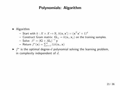
Polynomials Algorithm
I Algorithm
ndash Start with k X times X 7rarr R k(xxprime) = (xTxprime + 1)d
ndash Construct Gram matrix Gij = k(xixj) on the training samplesndash Solve β = (G + λId)minus1 yndash Return f(x) =
sumli=1 βik(xix)
I f is the optimal degree-d polynomial solving the learning problemin complexity independent of d
I What other forms of k correspond to linear learning inhigh-dimensional nonlinear embeddings of the data
21 36
Symmetric positive semi-definite functions
I Definition A function k X times X 7rarr R is psd if for any finitecollection of points x1 xl the l times l Gram matrix
Gij = k(xixj)
is positive semi-definite ie for any vector β isin Rl
βTGβ =sumij
βiβjk(xixj) ge 0
I Theorem[Mercer] If k is symmetric psd X is compact subset ofRn then it admits an eigenfunction decomposition
k(xxprime) =
Nsumi=1
λiφj(x)φj(xprime) = 〈Ψ(x)Ψ(xprime)〉l2
Ψ(x) = [ radicλjφ(x) ]T (3)
I Feature map associated with a kernel is not uniqueI Functional generalization of positive semi-definite matrices
22 36
Kernels
I Lineark(xxprime) = xTxprime
I Polynomialk(xxprime) = (xTxprime + 1)d
I Gaussian s =infin Universal
k(xxprime) = eminusxminusxprime2
2σ2
I Conic combinations
k(xxprime) = α1k1(xxprime) + α2k2(xxprime)
I Elementwise products
k(xxprime) = k1(xxprime)k2(xxprime)
I Kernels on discrete sets strings graphs sequences shapes
23 36
Gaussian Kernel is Positive Definite
I Exponential
eβxTxprime = 1 + βxTxprime +
β2
2(xTy)2 +
β3
3(xTy)3 +
I For any function f Rn 7rarr R psd function k the following kernelis psd
kprime(xxprime) = f(x) (k(xxprime)) f(xprime)
Proofsumij
βiβjkprime(xixj) =
sumij
βiβjf(xi)k(xixj)f(xj) =sumij
βprimeiβprimejk(xixj) ge 0
I Gaussian Kernel
k(xxprime) = eminusxminusxprime22
2σ2
= eminusx222σ2
(e
2xT xprime2σ2
)eminusxprime222σ2 (4)
24 36
The Mathematical Naturalness of Kernel Methods
I Data X isin Rd Models isin H X 7rarr R
I Geometry in H inner product 〈middot middot〉H norm middot H (Hilbert Spaces)I Theorem All nice Hilbert spaces are generated by a symmetric
positive definite function (the kernel) k(xxprime) on X times XI if f g isin H close ie f minus gH small then f(x) g(x) close forallx isin X I Reproducing Kernel Hilbert Spaces (RKHSs) Hilbert space H
that admit a reproducing kernel ie a function k(xxprime) satisfying
(i) forallx isin X k(middotx) isin H(ii) 〈f k(middotx)〉H = f(x)
I Reproducing kernels are symmetric psdsumij
βiβjk(xixj) = 〈sumi
βik(middotxi)sumi
βik(middotxi)〉H
= sumi
βik(middotxi)2H ge 0 (5)
I (Moore-Aronsjan 1950) Symmetric psd functions arereproducing kernels for some (unique) RKHS Hk
25 36
The Mathematical Naturalness of Kernel Methods
I Data X isin Rd Models isin H X 7rarr RI Geometry in H inner product 〈middot middot〉H norm middot H (Hilbert Spaces)
I Theorem All nice Hilbert spaces are generated by a symmetricpositive definite function (the kernel) k(xxprime) on X times X
I if f g isin H close ie f minus gH small then f(x) g(x) close forallx isin X I Reproducing Kernel Hilbert Spaces (RKHSs) Hilbert space H
that admit a reproducing kernel ie a function k(xxprime) satisfying
(i) forallx isin X k(middotx) isin H(ii) 〈f k(middotx)〉H = f(x)
I Reproducing kernels are symmetric psdsumij
βiβjk(xixj) = 〈sumi
βik(middotxi)sumi
βik(middotxi)〉H
= sumi
βik(middotxi)2H ge 0 (5)
I (Moore-Aronsjan 1950) Symmetric psd functions arereproducing kernels for some (unique) RKHS Hk
25 36
The Mathematical Naturalness of Kernel Methods
I Data X isin Rd Models isin H X 7rarr RI Geometry in H inner product 〈middot middot〉H norm middot H (Hilbert Spaces)I Theorem All nice Hilbert spaces are generated by a symmetric
positive definite function (the kernel) k(xxprime) on X times XI if f g isin H close ie f minus gH small then f(x) g(x) close forallx isin X
I Reproducing Kernel Hilbert Spaces (RKHSs) Hilbert space Hthat admit a reproducing kernel ie a function k(xxprime) satisfying
(i) forallx isin X k(middotx) isin H(ii) 〈f k(middotx)〉H = f(x)
I Reproducing kernels are symmetric psdsumij
βiβjk(xixj) = 〈sumi
βik(middotxi)sumi
βik(middotxi)〉H
= sumi
βik(middotxi)2H ge 0 (5)
I (Moore-Aronsjan 1950) Symmetric psd functions arereproducing kernels for some (unique) RKHS Hk
25 36
The Mathematical Naturalness of Kernel Methods
I Data X isin Rd Models isin H X 7rarr RI Geometry in H inner product 〈middot middot〉H norm middot H (Hilbert Spaces)I Theorem All nice Hilbert spaces are generated by a symmetric
positive definite function (the kernel) k(xxprime) on X times XI if f g isin H close ie f minus gH small then f(x) g(x) close forallx isin X I Reproducing Kernel Hilbert Spaces (RKHSs) Hilbert space H
that admit a reproducing kernel ie a function k(xxprime) satisfying
(i) forallx isin X k(middotx) isin H(ii) 〈f k(middotx)〉H = f(x)
I Reproducing kernels are symmetric psdsumij
βiβjk(xixj) = 〈sumi
βik(middotxi)sumi
βik(middotxi)〉H
= sumi
βik(middotxi)2H ge 0 (5)
I (Moore-Aronsjan 1950) Symmetric psd functions arereproducing kernels for some (unique) RKHS Hk
25 36
The Mathematical Naturalness of Kernel Methods
I Data X isin Rd Models isin H X 7rarr RI Geometry in H inner product 〈middot middot〉H norm middot H (Hilbert Spaces)I Theorem All nice Hilbert spaces are generated by a symmetric
positive definite function (the kernel) k(xxprime) on X times XI if f g isin H close ie f minus gH small then f(x) g(x) close forallx isin X I Reproducing Kernel Hilbert Spaces (RKHSs) Hilbert space H
that admit a reproducing kernel ie a function k(xxprime) satisfying
(i) forallx isin X k(middotx) isin H(ii) 〈f k(middotx)〉H = f(x)
I Reproducing kernels are symmetric psdsumij
βiβjk(xixj) = 〈sumi
βik(middotxi)sumi
βik(middotxi)〉H
= sumi
βik(middotxi)2H ge 0 (5)
I (Moore-Aronsjan 1950) Symmetric psd functions arereproducing kernels for some (unique) RKHS Hk 25 36
Kernel Methods Summary
I Symm pos def function k(x z) on input domain X sub Rd
I k hArr rich Reproducing Kernel Hilbert Space (RKHS) Hk ofreal-valued functions with inner product 〈middot middot〉k and norm middot k
I Regularized Risk Minimization hArr Linear models in an implicithigh-dimensional (often infinite-dimensional) feature space
f = arg minfisinHk
1
n
nsumi=1
V (yi f(xi)) + λf2Hk xi isin Rd
I Representer Theorem f(x) =sumni=1 αik(xxi)
26 36
Shallow and Deep Function Spaces
I What does it mean to understand a function space
ndash Linear f(x) = wTxw isin Rd
ndash Polynomial f(x) = wT Ψ(x)w isin Rs
ndash RKHS balls f isin Hk fk lt γ [like vM le 1]
I Shallow nets f(x) = wTσ(Wx) (w isin RdW isin Rs)ndash For srarrinfin W sim p σ(u) = eminusiu approximates Gaussian kernel
methodsndash Theorem [Bochner 1937] One-to-one correspondence between k
and a density p such that
k(x z) = ψ(xminus z) =
intRdeminusi(xminusz)Twp(w)dw asymp 1
s
ssumj=1
eminusi(xminusz)Twj
Gaussian kernel k(x z) = eminusxminusz22
2σ2 lArrrArr p = N (0 σminus2Id)ndash Similar integral approx relates ReLU to the arc-cosine kernelndash Optimization versus Randomization
27 36
Shallow and Deep Function Spaces
I What does it mean to understand a function space
ndash Linear f(x) = wTxw isin Rd
ndash Polynomial f(x) = wT Ψ(x)w isin Rs
ndash RKHS balls f isin Hk fk lt γ [like vM le 1]
I Shallow nets f(x) = wTσ(Wx) (w isin RdW isin Rs)ndash For srarrinfin W sim p σ(u) = eminusiu approximates Gaussian kernel
methodsndash Theorem [Bochner 1937] One-to-one correspondence between k
and a density p such that
k(x z) = ψ(xminus z) =
intRdeminusi(xminusz)Twp(w)dw asymp 1
s
ssumj=1
eminusi(xminusz)Twj
Gaussian kernel k(x z) = eminusxminusz22
2σ2 lArrrArr p = N (0 σminus2Id)ndash Similar integral approx relates ReLU to the arc-cosine kernelndash Optimization versus Randomization
27 36
Shallow and Deep Function Spaces
I What does it mean to understand a function space
ndash Linear f(x) = wTxw isin Rd
ndash Polynomial f(x) = wT Ψ(x)w isin Rs
ndash RKHS balls f isin Hk fk lt γ [like vM le 1]
I Shallow nets f(x) = wTσ(Wx) (w isin RdW isin Rs)ndash For srarrinfin W sim p σ(u) = eminusiu approximates Gaussian kernel
methodsndash Theorem [Bochner 1937] One-to-one correspondence between k
and a density p such that
k(x z) = ψ(xminus z) =
intRdeminusi(xminusz)Twp(w)dw asymp 1
s
ssumj=1
eminusi(xminusz)Twj
Gaussian kernel k(x z) = eminusxminusz22
2σ2 lArrrArr p = N (0 σminus2Id)ndash Similar integral approx relates ReLU to the arc-cosine kernelndash Optimization versus Randomization
27 36
Shallow and Deep Function Spaces
I What does it mean to understand a function space
ndash Linear f(x) = wTxw isin Rd
ndash Polynomial f(x) = wT Ψ(x)w isin Rs
ndash RKHS balls f isin Hk fk lt γ [like vM le 1]
I Shallow nets f(x) = wTσ(Wx) (w isin RdW isin Rs)
ndash For srarrinfin W sim p σ(u) = eminusiu approximates Gaussian kernelmethods
ndash Theorem [Bochner 1937] One-to-one correspondence between kand a density p such that
k(x z) = ψ(xminus z) =
intRdeminusi(xminusz)Twp(w)dw asymp 1
s
ssumj=1
eminusi(xminusz)Twj
Gaussian kernel k(x z) = eminusxminusz22
2σ2 lArrrArr p = N (0 σminus2Id)ndash Similar integral approx relates ReLU to the arc-cosine kernelndash Optimization versus Randomization
27 36
Shallow and Deep Function Spaces
I What does it mean to understand a function space
ndash Linear f(x) = wTxw isin Rd
ndash Polynomial f(x) = wT Ψ(x)w isin Rs
ndash RKHS balls f isin Hk fk lt γ [like vM le 1]
I Shallow nets f(x) = wTσ(Wx) (w isin RdW isin Rs)ndash For srarrinfin W sim p σ(u) = eminusiu approximates Gaussian kernel
methodsndash Theorem [Bochner 1937] One-to-one correspondence between k
and a density p such that
k(x z) = ψ(xminus z) =
intRdeminusi(xminusz)Twp(w)dw asymp 1
s
ssumj=1
eminusi(xminusz)Twj
Gaussian kernel k(x z) = eminusxminusz22
2σ2 lArrrArr p = N (0 σminus2Id)ndash Similar integral approx relates ReLU to the arc-cosine kernelndash Optimization versus Randomization
27 36
Expressivity of Deep Nets Linear Regions
I The ReLU map f(x) = max(Wx 0)W isin Rwtimesn is piecewise linear
I A piece is a connected region (a convex polytope) of Rd with sharedsparsity pattern in activations
I (Zaslavsky 1975) Number of linear regions formed by an arrangement of
s hyperplanes in d-dimensions in general position issumd
i=0
(si
)I Composition of ReLU maps is also piecewise linear
I (Raghu et al 2017 Pascano et al 2014 Montufar 2014) Number oflinear regions grows as O(wnd) for a composition of d ReLU maps(nrarr brarr brarr b rarr b) each of width w
I (Safran and Shamir 2017)
ndash 1[x le 1] x isin Rd ε-accurate 3-layer network with O(dε) neurons but cannot be approximated with
accuracy higher than O(1d4) using 2-layer networks unless width is exponential in d
28 36
Expressivity of Deep Nets Linear Regions
I The ReLU map f(x) = max(Wx 0)W isin Rwtimesn is piecewise linear
I A piece is a connected region (a convex polytope) of Rd with sharedsparsity pattern in activations
I (Zaslavsky 1975) Number of linear regions formed by an arrangement of
s hyperplanes in d-dimensions in general position issumd
i=0
(si
)I Composition of ReLU maps is also piecewise linear
I (Raghu et al 2017 Pascano et al 2014 Montufar 2014) Number oflinear regions grows as O(wnd) for a composition of d ReLU maps(nrarr brarr brarr b rarr b) each of width w
I (Safran and Shamir 2017)
ndash 1[x le 1] x isin Rd ε-accurate 3-layer network with O(dε) neurons but cannot be approximated with
accuracy higher than O(1d4) using 2-layer networks unless width is exponential in d
28 36
Expressivity of Deep Nets Linear Regions
I The ReLU map f(x) = max(Wx 0)W isin Rwtimesn is piecewise linear
I A piece is a connected region (a convex polytope) of Rd with sharedsparsity pattern in activations
I (Zaslavsky 1975) Number of linear regions formed by an arrangement of
s hyperplanes in d-dimensions in general position issumd
i=0
(si
)
I Composition of ReLU maps is also piecewise linear
I (Raghu et al 2017 Pascano et al 2014 Montufar 2014) Number oflinear regions grows as O(wnd) for a composition of d ReLU maps(nrarr brarr brarr b rarr b) each of width w
I (Safran and Shamir 2017)
ndash 1[x le 1] x isin Rd ε-accurate 3-layer network with O(dε) neurons but cannot be approximated with
accuracy higher than O(1d4) using 2-layer networks unless width is exponential in d
28 36
Expressivity of Deep Nets Linear Regions
I The ReLU map f(x) = max(Wx 0)W isin Rwtimesn is piecewise linear
I A piece is a connected region (a convex polytope) of Rd with sharedsparsity pattern in activations
I (Zaslavsky 1975) Number of linear regions formed by an arrangement of
s hyperplanes in d-dimensions in general position issumd
i=0
(si
)I Composition of ReLU maps is also piecewise linear
I (Raghu et al 2017 Pascano et al 2014 Montufar 2014) Number oflinear regions grows as O(wnd) for a composition of d ReLU maps(nrarr brarr brarr b rarr b) each of width w
I (Safran and Shamir 2017)
ndash 1[x le 1] x isin Rd ε-accurate 3-layer network with O(dε) neurons but cannot be approximated with
accuracy higher than O(1d4) using 2-layer networks unless width is exponential in d28 36
Expressivity of Deep Nets Trajectory Length
I (Raghu et al 2017) Trajectory Length (ldquogeneralized operator normrdquo)How much is a curve in the input space stretched by a layer in thenetwork
29 36
Expressivity of Deep Nets Trajectory Length
I (Raghu et al 2017) Trajectory Length (ldquogeneralized operator normrdquo)How much is a curve in the input space stretched by a layer in thenetwork
29 36
Expressivity and Generalization
I Expressiveness equiv capacity to fit random noise =rArr susceptibility tooverfitting (VC dimension Rademacher Complexity)
I Zhang et al 2017 Famous CNNs easily fit random labels
ndash Over-parameterized (n=12M psim 60M) but structuredndash Domain-knowledge baked in does not constraint expressiveness
I CNNs tend to generalize even without regularization (explicit and implicit)
I For linear regression SGD returns minimum norm solution
30 36
Expressivity and Generalization
I Expressiveness equiv capacity to fit random noise =rArr susceptibility tooverfitting (VC dimension Rademacher Complexity)
I Zhang et al 2017 Famous CNNs easily fit random labels
ndash Over-parameterized (n=12M psim 60M) but structuredndash Domain-knowledge baked in does not constraint expressiveness
I CNNs tend to generalize even without regularization (explicit and implicit)
I For linear regression SGD returns minimum norm solution
30 36
Expressivity and Generalization
I Expressiveness equiv capacity to fit random noise =rArr susceptibility tooverfitting (VC dimension Rademacher Complexity)
I Zhang et al 2017 Famous CNNs easily fit random labels
ndash Over-parameterized (n=12M psim 60M) but structuredndash Domain-knowledge baked in does not constraint expressiveness
I CNNs tend to generalize even without regularization (explicit and implicit)
I For linear regression SGD returns minimum norm solution
30 36
Optimization Landscape Symmetry and Saddle Points
I Folklore lots of equivalent good local minI Classification of critical points based on Hessian spectrumI Permutation and Scaling symmetries
I Thm [Lee et al 2016 Anadkumar Ge] For the short-step gradientmethod the basin of attraction of strict saddle points (atleast onenegative eigenvalue) has measure zero
31 36
Optimization Landscape Symmetry and Saddle Points
I Folklore lots of equivalent good local minI Classification of critical points based on Hessian spectrumI Permutation and Scaling symmetries
I Thm [Lee et al 2016 Anadkumar Ge] For the short-step gradientmethod the basin of attraction of strict saddle points (atleast onenegative eigenvalue) has measure zero
31 36
Optimization Landscape Symmetry and Saddle Points
I Folklore lots of equivalent good local minI Classification of critical points based on Hessian spectrumI Permutation and Scaling symmetries
I Thm [Lee et al 2016 Anadkumar Ge] For the short-step gradientmethod the basin of attraction of strict saddle points (atleast onenegative eigenvalue) has measure zero
31 36
Optimization Landscape Sharp Minima and Stability
Keskar et al 2017 On large-batch training for DL Generalization Gap and Sharp Minima
32 36
Deep Learning Computational Graphs TensorFlow
tensorfloworg
I Tensors-in Tensors-out
I Evergrowing list of Tensor-Ops (PythonC++)
f(xw)
[partf
partx
]T v
[partf
partw
]T v
I Automatic Differentiation Reverse mode
partxL
partxi=sumirarrj
partxL
partxj
partxj
partxi
33 36
Computational Graphs and TensorFlow
tensorfloworg
I SGD with minibatches
wk+1 = wk minus ηlsumi=1
partli
partw
∣∣∣wt
I Model Parallelism Assign independent paths tothreads GPUs
I Data Parallelism create Graph replicas on differentmachines
I Mobile TensorFlow
34 36
Computational Graphs and TensorFlow
tensorfloworg
35 36
Computational Graphs and TensorFlow
tensorfloworg
35 36
Computational Graphs and TensorFlow
tensorfloworg
35 36
Challenges and Opportunities
I Lots of fascinating unsolved problems
I Can you win Imagenet with Convex optimization
I Tools from polynomial optimization (global optimization deep-RL)
I Supervised to Semi-supervised to Unsupervised Learning
I Compact efficient real-time models (eliminateover-parametrization) for new form factors
I Exciting emerging world of Robotics Wearable ComputersIntelligent home devices Personal digital assistants
Google Internship Program
36 36
- anm0
- fdrm0
- fdrm5

Polynomials Algorithm
I Algorithm
ndash Start with k X times X 7rarr R k(xxprime) = (xTxprime + 1)d
ndash Construct Gram matrix Gij = k(xixj) on the training samplesndash Solve β = (G + λId)minus1 yndash Return f(x) =
sumli=1 βik(xix)
I f is the optimal degree-d polynomial solving the learning problemin complexity independent of d
I What other forms of k correspond to linear learning inhigh-dimensional nonlinear embeddings of the data
21 36
Symmetric positive semi-definite functions
I Definition A function k X times X 7rarr R is psd if for any finitecollection of points x1 xl the l times l Gram matrix
Gij = k(xixj)
is positive semi-definite ie for any vector β isin Rl
βTGβ =sumij
βiβjk(xixj) ge 0
I Theorem[Mercer] If k is symmetric psd X is compact subset ofRn then it admits an eigenfunction decomposition
k(xxprime) =
Nsumi=1
λiφj(x)φj(xprime) = 〈Ψ(x)Ψ(xprime)〉l2
Ψ(x) = [ radicλjφ(x) ]T (3)
I Feature map associated with a kernel is not uniqueI Functional generalization of positive semi-definite matrices
22 36
Kernels
I Lineark(xxprime) = xTxprime
I Polynomialk(xxprime) = (xTxprime + 1)d
I Gaussian s =infin Universal
k(xxprime) = eminusxminusxprime2
2σ2
I Conic combinations
k(xxprime) = α1k1(xxprime) + α2k2(xxprime)
I Elementwise products
k(xxprime) = k1(xxprime)k2(xxprime)
I Kernels on discrete sets strings graphs sequences shapes
23 36
Gaussian Kernel is Positive Definite
I Exponential
eβxTxprime = 1 + βxTxprime +
β2
2(xTy)2 +
β3
3(xTy)3 +
I For any function f Rn 7rarr R psd function k the following kernelis psd
kprime(xxprime) = f(x) (k(xxprime)) f(xprime)
Proofsumij
βiβjkprime(xixj) =
sumij
βiβjf(xi)k(xixj)f(xj) =sumij
βprimeiβprimejk(xixj) ge 0
I Gaussian Kernel
k(xxprime) = eminusxminusxprime22
2σ2
= eminusx222σ2
(e
2xT xprime2σ2
)eminusxprime222σ2 (4)
24 36
The Mathematical Naturalness of Kernel Methods
I Data X isin Rd Models isin H X 7rarr R
I Geometry in H inner product 〈middot middot〉H norm middot H (Hilbert Spaces)I Theorem All nice Hilbert spaces are generated by a symmetric
positive definite function (the kernel) k(xxprime) on X times XI if f g isin H close ie f minus gH small then f(x) g(x) close forallx isin X I Reproducing Kernel Hilbert Spaces (RKHSs) Hilbert space H
that admit a reproducing kernel ie a function k(xxprime) satisfying
(i) forallx isin X k(middotx) isin H(ii) 〈f k(middotx)〉H = f(x)
I Reproducing kernels are symmetric psdsumij
βiβjk(xixj) = 〈sumi
βik(middotxi)sumi
βik(middotxi)〉H
= sumi
βik(middotxi)2H ge 0 (5)
I (Moore-Aronsjan 1950) Symmetric psd functions arereproducing kernels for some (unique) RKHS Hk
25 36
The Mathematical Naturalness of Kernel Methods
I Data X isin Rd Models isin H X 7rarr RI Geometry in H inner product 〈middot middot〉H norm middot H (Hilbert Spaces)
I Theorem All nice Hilbert spaces are generated by a symmetricpositive definite function (the kernel) k(xxprime) on X times X
I if f g isin H close ie f minus gH small then f(x) g(x) close forallx isin X I Reproducing Kernel Hilbert Spaces (RKHSs) Hilbert space H
that admit a reproducing kernel ie a function k(xxprime) satisfying
(i) forallx isin X k(middotx) isin H(ii) 〈f k(middotx)〉H = f(x)
I Reproducing kernels are symmetric psdsumij
βiβjk(xixj) = 〈sumi
βik(middotxi)sumi
βik(middotxi)〉H
= sumi
βik(middotxi)2H ge 0 (5)
I (Moore-Aronsjan 1950) Symmetric psd functions arereproducing kernels for some (unique) RKHS Hk
25 36
The Mathematical Naturalness of Kernel Methods
I Data X isin Rd Models isin H X 7rarr RI Geometry in H inner product 〈middot middot〉H norm middot H (Hilbert Spaces)I Theorem All nice Hilbert spaces are generated by a symmetric
positive definite function (the kernel) k(xxprime) on X times XI if f g isin H close ie f minus gH small then f(x) g(x) close forallx isin X
I Reproducing Kernel Hilbert Spaces (RKHSs) Hilbert space Hthat admit a reproducing kernel ie a function k(xxprime) satisfying
(i) forallx isin X k(middotx) isin H(ii) 〈f k(middotx)〉H = f(x)
I Reproducing kernels are symmetric psdsumij
βiβjk(xixj) = 〈sumi
βik(middotxi)sumi
βik(middotxi)〉H
= sumi
βik(middotxi)2H ge 0 (5)
I (Moore-Aronsjan 1950) Symmetric psd functions arereproducing kernels for some (unique) RKHS Hk
25 36
The Mathematical Naturalness of Kernel Methods
I Data X isin Rd Models isin H X 7rarr RI Geometry in H inner product 〈middot middot〉H norm middot H (Hilbert Spaces)I Theorem All nice Hilbert spaces are generated by a symmetric
positive definite function (the kernel) k(xxprime) on X times XI if f g isin H close ie f minus gH small then f(x) g(x) close forallx isin X I Reproducing Kernel Hilbert Spaces (RKHSs) Hilbert space H
that admit a reproducing kernel ie a function k(xxprime) satisfying
(i) forallx isin X k(middotx) isin H(ii) 〈f k(middotx)〉H = f(x)
I Reproducing kernels are symmetric psdsumij
βiβjk(xixj) = 〈sumi
βik(middotxi)sumi
βik(middotxi)〉H
= sumi
βik(middotxi)2H ge 0 (5)
I (Moore-Aronsjan 1950) Symmetric psd functions arereproducing kernels for some (unique) RKHS Hk
25 36
The Mathematical Naturalness of Kernel Methods
I Data X isin Rd Models isin H X 7rarr RI Geometry in H inner product 〈middot middot〉H norm middot H (Hilbert Spaces)I Theorem All nice Hilbert spaces are generated by a symmetric
positive definite function (the kernel) k(xxprime) on X times XI if f g isin H close ie f minus gH small then f(x) g(x) close forallx isin X I Reproducing Kernel Hilbert Spaces (RKHSs) Hilbert space H
that admit a reproducing kernel ie a function k(xxprime) satisfying
(i) forallx isin X k(middotx) isin H(ii) 〈f k(middotx)〉H = f(x)
I Reproducing kernels are symmetric psdsumij
βiβjk(xixj) = 〈sumi
βik(middotxi)sumi
βik(middotxi)〉H
= sumi
βik(middotxi)2H ge 0 (5)
I (Moore-Aronsjan 1950) Symmetric psd functions arereproducing kernels for some (unique) RKHS Hk 25 36
Kernel Methods Summary
I Symm pos def function k(x z) on input domain X sub Rd
I k hArr rich Reproducing Kernel Hilbert Space (RKHS) Hk ofreal-valued functions with inner product 〈middot middot〉k and norm middot k
I Regularized Risk Minimization hArr Linear models in an implicithigh-dimensional (often infinite-dimensional) feature space
f = arg minfisinHk
1
n
nsumi=1
V (yi f(xi)) + λf2Hk xi isin Rd
I Representer Theorem f(x) =sumni=1 αik(xxi)
26 36
Shallow and Deep Function Spaces
I What does it mean to understand a function space
ndash Linear f(x) = wTxw isin Rd
ndash Polynomial f(x) = wT Ψ(x)w isin Rs
ndash RKHS balls f isin Hk fk lt γ [like vM le 1]
I Shallow nets f(x) = wTσ(Wx) (w isin RdW isin Rs)ndash For srarrinfin W sim p σ(u) = eminusiu approximates Gaussian kernel
methodsndash Theorem [Bochner 1937] One-to-one correspondence between k
and a density p such that
k(x z) = ψ(xminus z) =
intRdeminusi(xminusz)Twp(w)dw asymp 1
s
ssumj=1
eminusi(xminusz)Twj
Gaussian kernel k(x z) = eminusxminusz22
2σ2 lArrrArr p = N (0 σminus2Id)ndash Similar integral approx relates ReLU to the arc-cosine kernelndash Optimization versus Randomization
27 36
Shallow and Deep Function Spaces
I What does it mean to understand a function space
ndash Linear f(x) = wTxw isin Rd
ndash Polynomial f(x) = wT Ψ(x)w isin Rs
ndash RKHS balls f isin Hk fk lt γ [like vM le 1]
I Shallow nets f(x) = wTσ(Wx) (w isin RdW isin Rs)ndash For srarrinfin W sim p σ(u) = eminusiu approximates Gaussian kernel
methodsndash Theorem [Bochner 1937] One-to-one correspondence between k
and a density p such that
k(x z) = ψ(xminus z) =
intRdeminusi(xminusz)Twp(w)dw asymp 1
s
ssumj=1
eminusi(xminusz)Twj
Gaussian kernel k(x z) = eminusxminusz22
2σ2 lArrrArr p = N (0 σminus2Id)ndash Similar integral approx relates ReLU to the arc-cosine kernelndash Optimization versus Randomization
27 36
Shallow and Deep Function Spaces
I What does it mean to understand a function space
ndash Linear f(x) = wTxw isin Rd
ndash Polynomial f(x) = wT Ψ(x)w isin Rs
ndash RKHS balls f isin Hk fk lt γ [like vM le 1]
I Shallow nets f(x) = wTσ(Wx) (w isin RdW isin Rs)ndash For srarrinfin W sim p σ(u) = eminusiu approximates Gaussian kernel
methodsndash Theorem [Bochner 1937] One-to-one correspondence between k
and a density p such that
k(x z) = ψ(xminus z) =
intRdeminusi(xminusz)Twp(w)dw asymp 1
s
ssumj=1
eminusi(xminusz)Twj
Gaussian kernel k(x z) = eminusxminusz22
2σ2 lArrrArr p = N (0 σminus2Id)ndash Similar integral approx relates ReLU to the arc-cosine kernelndash Optimization versus Randomization
27 36
Shallow and Deep Function Spaces
I What does it mean to understand a function space
ndash Linear f(x) = wTxw isin Rd
ndash Polynomial f(x) = wT Ψ(x)w isin Rs
ndash RKHS balls f isin Hk fk lt γ [like vM le 1]
I Shallow nets f(x) = wTσ(Wx) (w isin RdW isin Rs)
ndash For srarrinfin W sim p σ(u) = eminusiu approximates Gaussian kernelmethods
ndash Theorem [Bochner 1937] One-to-one correspondence between kand a density p such that
k(x z) = ψ(xminus z) =
intRdeminusi(xminusz)Twp(w)dw asymp 1
s
ssumj=1
eminusi(xminusz)Twj
Gaussian kernel k(x z) = eminusxminusz22
2σ2 lArrrArr p = N (0 σminus2Id)ndash Similar integral approx relates ReLU to the arc-cosine kernelndash Optimization versus Randomization
27 36
Shallow and Deep Function Spaces
I What does it mean to understand a function space
ndash Linear f(x) = wTxw isin Rd
ndash Polynomial f(x) = wT Ψ(x)w isin Rs
ndash RKHS balls f isin Hk fk lt γ [like vM le 1]
I Shallow nets f(x) = wTσ(Wx) (w isin RdW isin Rs)ndash For srarrinfin W sim p σ(u) = eminusiu approximates Gaussian kernel
methodsndash Theorem [Bochner 1937] One-to-one correspondence between k
and a density p such that
k(x z) = ψ(xminus z) =
intRdeminusi(xminusz)Twp(w)dw asymp 1
s
ssumj=1
eminusi(xminusz)Twj
Gaussian kernel k(x z) = eminusxminusz22
2σ2 lArrrArr p = N (0 σminus2Id)ndash Similar integral approx relates ReLU to the arc-cosine kernelndash Optimization versus Randomization
27 36
Expressivity of Deep Nets Linear Regions
I The ReLU map f(x) = max(Wx 0)W isin Rwtimesn is piecewise linear
I A piece is a connected region (a convex polytope) of Rd with sharedsparsity pattern in activations
I (Zaslavsky 1975) Number of linear regions formed by an arrangement of
s hyperplanes in d-dimensions in general position issumd
i=0
(si
)I Composition of ReLU maps is also piecewise linear
I (Raghu et al 2017 Pascano et al 2014 Montufar 2014) Number oflinear regions grows as O(wnd) for a composition of d ReLU maps(nrarr brarr brarr b rarr b) each of width w
I (Safran and Shamir 2017)
ndash 1[x le 1] x isin Rd ε-accurate 3-layer network with O(dε) neurons but cannot be approximated with
accuracy higher than O(1d4) using 2-layer networks unless width is exponential in d
28 36
Expressivity of Deep Nets Linear Regions
I The ReLU map f(x) = max(Wx 0)W isin Rwtimesn is piecewise linear
I A piece is a connected region (a convex polytope) of Rd with sharedsparsity pattern in activations
I (Zaslavsky 1975) Number of linear regions formed by an arrangement of
s hyperplanes in d-dimensions in general position issumd
i=0
(si
)I Composition of ReLU maps is also piecewise linear
I (Raghu et al 2017 Pascano et al 2014 Montufar 2014) Number oflinear regions grows as O(wnd) for a composition of d ReLU maps(nrarr brarr brarr b rarr b) each of width w
I (Safran and Shamir 2017)
ndash 1[x le 1] x isin Rd ε-accurate 3-layer network with O(dε) neurons but cannot be approximated with
accuracy higher than O(1d4) using 2-layer networks unless width is exponential in d
28 36
Expressivity of Deep Nets Linear Regions
I The ReLU map f(x) = max(Wx 0)W isin Rwtimesn is piecewise linear
I A piece is a connected region (a convex polytope) of Rd with sharedsparsity pattern in activations
I (Zaslavsky 1975) Number of linear regions formed by an arrangement of
s hyperplanes in d-dimensions in general position issumd
i=0
(si
)
I Composition of ReLU maps is also piecewise linear
I (Raghu et al 2017 Pascano et al 2014 Montufar 2014) Number oflinear regions grows as O(wnd) for a composition of d ReLU maps(nrarr brarr brarr b rarr b) each of width w
I (Safran and Shamir 2017)
ndash 1[x le 1] x isin Rd ε-accurate 3-layer network with O(dε) neurons but cannot be approximated with
accuracy higher than O(1d4) using 2-layer networks unless width is exponential in d
28 36
Expressivity of Deep Nets Linear Regions
I The ReLU map f(x) = max(Wx 0)W isin Rwtimesn is piecewise linear
I A piece is a connected region (a convex polytope) of Rd with sharedsparsity pattern in activations
I (Zaslavsky 1975) Number of linear regions formed by an arrangement of
s hyperplanes in d-dimensions in general position issumd
i=0
(si
)I Composition of ReLU maps is also piecewise linear
I (Raghu et al 2017 Pascano et al 2014 Montufar 2014) Number oflinear regions grows as O(wnd) for a composition of d ReLU maps(nrarr brarr brarr b rarr b) each of width w
I (Safran and Shamir 2017)
ndash 1[x le 1] x isin Rd ε-accurate 3-layer network with O(dε) neurons but cannot be approximated with
accuracy higher than O(1d4) using 2-layer networks unless width is exponential in d28 36
Expressivity of Deep Nets Trajectory Length
I (Raghu et al 2017) Trajectory Length (ldquogeneralized operator normrdquo)How much is a curve in the input space stretched by a layer in thenetwork
29 36
Expressivity of Deep Nets Trajectory Length
I (Raghu et al 2017) Trajectory Length (ldquogeneralized operator normrdquo)How much is a curve in the input space stretched by a layer in thenetwork
29 36
Expressivity and Generalization
I Expressiveness equiv capacity to fit random noise =rArr susceptibility tooverfitting (VC dimension Rademacher Complexity)
I Zhang et al 2017 Famous CNNs easily fit random labels
ndash Over-parameterized (n=12M psim 60M) but structuredndash Domain-knowledge baked in does not constraint expressiveness
I CNNs tend to generalize even without regularization (explicit and implicit)
I For linear regression SGD returns minimum norm solution
30 36
Expressivity and Generalization
I Expressiveness equiv capacity to fit random noise =rArr susceptibility tooverfitting (VC dimension Rademacher Complexity)
I Zhang et al 2017 Famous CNNs easily fit random labels
ndash Over-parameterized (n=12M psim 60M) but structuredndash Domain-knowledge baked in does not constraint expressiveness
I CNNs tend to generalize even without regularization (explicit and implicit)
I For linear regression SGD returns minimum norm solution
30 36
Expressivity and Generalization
I Expressiveness equiv capacity to fit random noise =rArr susceptibility tooverfitting (VC dimension Rademacher Complexity)
I Zhang et al 2017 Famous CNNs easily fit random labels
ndash Over-parameterized (n=12M psim 60M) but structuredndash Domain-knowledge baked in does not constraint expressiveness
I CNNs tend to generalize even without regularization (explicit and implicit)
I For linear regression SGD returns minimum norm solution
30 36
Optimization Landscape Symmetry and Saddle Points
I Folklore lots of equivalent good local minI Classification of critical points based on Hessian spectrumI Permutation and Scaling symmetries
I Thm [Lee et al 2016 Anadkumar Ge] For the short-step gradientmethod the basin of attraction of strict saddle points (atleast onenegative eigenvalue) has measure zero
31 36
Optimization Landscape Symmetry and Saddle Points
I Folklore lots of equivalent good local minI Classification of critical points based on Hessian spectrumI Permutation and Scaling symmetries
I Thm [Lee et al 2016 Anadkumar Ge] For the short-step gradientmethod the basin of attraction of strict saddle points (atleast onenegative eigenvalue) has measure zero
31 36
Optimization Landscape Symmetry and Saddle Points
I Folklore lots of equivalent good local minI Classification of critical points based on Hessian spectrumI Permutation and Scaling symmetries
I Thm [Lee et al 2016 Anadkumar Ge] For the short-step gradientmethod the basin of attraction of strict saddle points (atleast onenegative eigenvalue) has measure zero
31 36
Optimization Landscape Sharp Minima and Stability
Keskar et al 2017 On large-batch training for DL Generalization Gap and Sharp Minima
32 36
Deep Learning Computational Graphs TensorFlow
tensorfloworg
I Tensors-in Tensors-out
I Evergrowing list of Tensor-Ops (PythonC++)
f(xw)
[partf
partx
]T v
[partf
partw
]T v
I Automatic Differentiation Reverse mode
partxL
partxi=sumirarrj
partxL
partxj
partxj
partxi
33 36
Computational Graphs and TensorFlow
tensorfloworg
I SGD with minibatches
wk+1 = wk minus ηlsumi=1
partli
partw
∣∣∣wt
I Model Parallelism Assign independent paths tothreads GPUs
I Data Parallelism create Graph replicas on differentmachines
I Mobile TensorFlow
34 36
Computational Graphs and TensorFlow
tensorfloworg
35 36
Computational Graphs and TensorFlow
tensorfloworg
35 36
Computational Graphs and TensorFlow
tensorfloworg
35 36
Challenges and Opportunities
I Lots of fascinating unsolved problems
I Can you win Imagenet with Convex optimization
I Tools from polynomial optimization (global optimization deep-RL)
I Supervised to Semi-supervised to Unsupervised Learning
I Compact efficient real-time models (eliminateover-parametrization) for new form factors
I Exciting emerging world of Robotics Wearable ComputersIntelligent home devices Personal digital assistants
Google Internship Program
36 36
- anm0
- fdrm0
- fdrm5
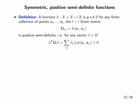
Symmetric positive semi-definite functions
I Definition A function k X times X 7rarr R is psd if for any finitecollection of points x1 xl the l times l Gram matrix
Gij = k(xixj)
is positive semi-definite ie for any vector β isin Rl
βTGβ =sumij
βiβjk(xixj) ge 0
I Theorem[Mercer] If k is symmetric psd X is compact subset ofRn then it admits an eigenfunction decomposition
k(xxprime) =
Nsumi=1
λiφj(x)φj(xprime) = 〈Ψ(x)Ψ(xprime)〉l2
Ψ(x) = [ radicλjφ(x) ]T (3)
I Feature map associated with a kernel is not uniqueI Functional generalization of positive semi-definite matrices
22 36
Kernels
I Lineark(xxprime) = xTxprime
I Polynomialk(xxprime) = (xTxprime + 1)d
I Gaussian s =infin Universal
k(xxprime) = eminusxminusxprime2
2σ2
I Conic combinations
k(xxprime) = α1k1(xxprime) + α2k2(xxprime)
I Elementwise products
k(xxprime) = k1(xxprime)k2(xxprime)
I Kernels on discrete sets strings graphs sequences shapes
23 36
Gaussian Kernel is Positive Definite
I Exponential
eβxTxprime = 1 + βxTxprime +
β2
2(xTy)2 +
β3
3(xTy)3 +
I For any function f Rn 7rarr R psd function k the following kernelis psd
kprime(xxprime) = f(x) (k(xxprime)) f(xprime)
Proofsumij
βiβjkprime(xixj) =
sumij
βiβjf(xi)k(xixj)f(xj) =sumij
βprimeiβprimejk(xixj) ge 0
I Gaussian Kernel
k(xxprime) = eminusxminusxprime22
2σ2
= eminusx222σ2
(e
2xT xprime2σ2
)eminusxprime222σ2 (4)
24 36
The Mathematical Naturalness of Kernel Methods
I Data X isin Rd Models isin H X 7rarr R
I Geometry in H inner product 〈middot middot〉H norm middot H (Hilbert Spaces)I Theorem All nice Hilbert spaces are generated by a symmetric
positive definite function (the kernel) k(xxprime) on X times XI if f g isin H close ie f minus gH small then f(x) g(x) close forallx isin X I Reproducing Kernel Hilbert Spaces (RKHSs) Hilbert space H
that admit a reproducing kernel ie a function k(xxprime) satisfying
(i) forallx isin X k(middotx) isin H(ii) 〈f k(middotx)〉H = f(x)
I Reproducing kernels are symmetric psdsumij
βiβjk(xixj) = 〈sumi
βik(middotxi)sumi
βik(middotxi)〉H
= sumi
βik(middotxi)2H ge 0 (5)
I (Moore-Aronsjan 1950) Symmetric psd functions arereproducing kernels for some (unique) RKHS Hk
25 36
The Mathematical Naturalness of Kernel Methods
I Data X isin Rd Models isin H X 7rarr RI Geometry in H inner product 〈middot middot〉H norm middot H (Hilbert Spaces)
I Theorem All nice Hilbert spaces are generated by a symmetricpositive definite function (the kernel) k(xxprime) on X times X
I if f g isin H close ie f minus gH small then f(x) g(x) close forallx isin X I Reproducing Kernel Hilbert Spaces (RKHSs) Hilbert space H
that admit a reproducing kernel ie a function k(xxprime) satisfying
(i) forallx isin X k(middotx) isin H(ii) 〈f k(middotx)〉H = f(x)
I Reproducing kernels are symmetric psdsumij
βiβjk(xixj) = 〈sumi
βik(middotxi)sumi
βik(middotxi)〉H
= sumi
βik(middotxi)2H ge 0 (5)
I (Moore-Aronsjan 1950) Symmetric psd functions arereproducing kernels for some (unique) RKHS Hk
25 36
The Mathematical Naturalness of Kernel Methods
I Data X isin Rd Models isin H X 7rarr RI Geometry in H inner product 〈middot middot〉H norm middot H (Hilbert Spaces)I Theorem All nice Hilbert spaces are generated by a symmetric
positive definite function (the kernel) k(xxprime) on X times XI if f g isin H close ie f minus gH small then f(x) g(x) close forallx isin X
I Reproducing Kernel Hilbert Spaces (RKHSs) Hilbert space Hthat admit a reproducing kernel ie a function k(xxprime) satisfying
(i) forallx isin X k(middotx) isin H(ii) 〈f k(middotx)〉H = f(x)
I Reproducing kernels are symmetric psdsumij
βiβjk(xixj) = 〈sumi
βik(middotxi)sumi
βik(middotxi)〉H
= sumi
βik(middotxi)2H ge 0 (5)
I (Moore-Aronsjan 1950) Symmetric psd functions arereproducing kernels for some (unique) RKHS Hk
25 36
The Mathematical Naturalness of Kernel Methods
I Data X isin Rd Models isin H X 7rarr RI Geometry in H inner product 〈middot middot〉H norm middot H (Hilbert Spaces)I Theorem All nice Hilbert spaces are generated by a symmetric
positive definite function (the kernel) k(xxprime) on X times XI if f g isin H close ie f minus gH small then f(x) g(x) close forallx isin X I Reproducing Kernel Hilbert Spaces (RKHSs) Hilbert space H
that admit a reproducing kernel ie a function k(xxprime) satisfying
(i) forallx isin X k(middotx) isin H(ii) 〈f k(middotx)〉H = f(x)
I Reproducing kernels are symmetric psdsumij
βiβjk(xixj) = 〈sumi
βik(middotxi)sumi
βik(middotxi)〉H
= sumi
βik(middotxi)2H ge 0 (5)
I (Moore-Aronsjan 1950) Symmetric psd functions arereproducing kernels for some (unique) RKHS Hk
25 36
The Mathematical Naturalness of Kernel Methods
I Data X isin Rd Models isin H X 7rarr RI Geometry in H inner product 〈middot middot〉H norm middot H (Hilbert Spaces)I Theorem All nice Hilbert spaces are generated by a symmetric
positive definite function (the kernel) k(xxprime) on X times XI if f g isin H close ie f minus gH small then f(x) g(x) close forallx isin X I Reproducing Kernel Hilbert Spaces (RKHSs) Hilbert space H
that admit a reproducing kernel ie a function k(xxprime) satisfying
(i) forallx isin X k(middotx) isin H(ii) 〈f k(middotx)〉H = f(x)
I Reproducing kernels are symmetric psdsumij
βiβjk(xixj) = 〈sumi
βik(middotxi)sumi
βik(middotxi)〉H
= sumi
βik(middotxi)2H ge 0 (5)
I (Moore-Aronsjan 1950) Symmetric psd functions arereproducing kernels for some (unique) RKHS Hk 25 36
Kernel Methods Summary
I Symm pos def function k(x z) on input domain X sub Rd
I k hArr rich Reproducing Kernel Hilbert Space (RKHS) Hk ofreal-valued functions with inner product 〈middot middot〉k and norm middot k
I Regularized Risk Minimization hArr Linear models in an implicithigh-dimensional (often infinite-dimensional) feature space
f = arg minfisinHk
1
n
nsumi=1
V (yi f(xi)) + λf2Hk xi isin Rd
I Representer Theorem f(x) =sumni=1 αik(xxi)
26 36
Shallow and Deep Function Spaces
I What does it mean to understand a function space
ndash Linear f(x) = wTxw isin Rd
ndash Polynomial f(x) = wT Ψ(x)w isin Rs
ndash RKHS balls f isin Hk fk lt γ [like vM le 1]
I Shallow nets f(x) = wTσ(Wx) (w isin RdW isin Rs)ndash For srarrinfin W sim p σ(u) = eminusiu approximates Gaussian kernel
methodsndash Theorem [Bochner 1937] One-to-one correspondence between k
and a density p such that
k(x z) = ψ(xminus z) =
intRdeminusi(xminusz)Twp(w)dw asymp 1
s
ssumj=1
eminusi(xminusz)Twj
Gaussian kernel k(x z) = eminusxminusz22
2σ2 lArrrArr p = N (0 σminus2Id)ndash Similar integral approx relates ReLU to the arc-cosine kernelndash Optimization versus Randomization
27 36
Shallow and Deep Function Spaces
I What does it mean to understand a function space
ndash Linear f(x) = wTxw isin Rd
ndash Polynomial f(x) = wT Ψ(x)w isin Rs
ndash RKHS balls f isin Hk fk lt γ [like vM le 1]
I Shallow nets f(x) = wTσ(Wx) (w isin RdW isin Rs)ndash For srarrinfin W sim p σ(u) = eminusiu approximates Gaussian kernel
methodsndash Theorem [Bochner 1937] One-to-one correspondence between k
and a density p such that
k(x z) = ψ(xminus z) =
intRdeminusi(xminusz)Twp(w)dw asymp 1
s
ssumj=1
eminusi(xminusz)Twj
Gaussian kernel k(x z) = eminusxminusz22
2σ2 lArrrArr p = N (0 σminus2Id)ndash Similar integral approx relates ReLU to the arc-cosine kernelndash Optimization versus Randomization
27 36
Shallow and Deep Function Spaces
I What does it mean to understand a function space
ndash Linear f(x) = wTxw isin Rd
ndash Polynomial f(x) = wT Ψ(x)w isin Rs
ndash RKHS balls f isin Hk fk lt γ [like vM le 1]
I Shallow nets f(x) = wTσ(Wx) (w isin RdW isin Rs)ndash For srarrinfin W sim p σ(u) = eminusiu approximates Gaussian kernel
methodsndash Theorem [Bochner 1937] One-to-one correspondence between k
and a density p such that
k(x z) = ψ(xminus z) =
intRdeminusi(xminusz)Twp(w)dw asymp 1
s
ssumj=1
eminusi(xminusz)Twj
Gaussian kernel k(x z) = eminusxminusz22
2σ2 lArrrArr p = N (0 σminus2Id)ndash Similar integral approx relates ReLU to the arc-cosine kernelndash Optimization versus Randomization
27 36
Shallow and Deep Function Spaces
I What does it mean to understand a function space
ndash Linear f(x) = wTxw isin Rd
ndash Polynomial f(x) = wT Ψ(x)w isin Rs
ndash RKHS balls f isin Hk fk lt γ [like vM le 1]
I Shallow nets f(x) = wTσ(Wx) (w isin RdW isin Rs)
ndash For srarrinfin W sim p σ(u) = eminusiu approximates Gaussian kernelmethods
ndash Theorem [Bochner 1937] One-to-one correspondence between kand a density p such that
k(x z) = ψ(xminus z) =
intRdeminusi(xminusz)Twp(w)dw asymp 1
s
ssumj=1
eminusi(xminusz)Twj
Gaussian kernel k(x z) = eminusxminusz22
2σ2 lArrrArr p = N (0 σminus2Id)ndash Similar integral approx relates ReLU to the arc-cosine kernelndash Optimization versus Randomization
27 36
Shallow and Deep Function Spaces
I What does it mean to understand a function space
ndash Linear f(x) = wTxw isin Rd
ndash Polynomial f(x) = wT Ψ(x)w isin Rs
ndash RKHS balls f isin Hk fk lt γ [like vM le 1]
I Shallow nets f(x) = wTσ(Wx) (w isin RdW isin Rs)ndash For srarrinfin W sim p σ(u) = eminusiu approximates Gaussian kernel
methodsndash Theorem [Bochner 1937] One-to-one correspondence between k
and a density p such that
k(x z) = ψ(xminus z) =
intRdeminusi(xminusz)Twp(w)dw asymp 1
s
ssumj=1
eminusi(xminusz)Twj
Gaussian kernel k(x z) = eminusxminusz22
2σ2 lArrrArr p = N (0 σminus2Id)ndash Similar integral approx relates ReLU to the arc-cosine kernelndash Optimization versus Randomization
27 36
Expressivity of Deep Nets Linear Regions
I The ReLU map f(x) = max(Wx 0)W isin Rwtimesn is piecewise linear
I A piece is a connected region (a convex polytope) of Rd with sharedsparsity pattern in activations
I (Zaslavsky 1975) Number of linear regions formed by an arrangement of
s hyperplanes in d-dimensions in general position issumd
i=0
(si
)I Composition of ReLU maps is also piecewise linear
I (Raghu et al 2017 Pascano et al 2014 Montufar 2014) Number oflinear regions grows as O(wnd) for a composition of d ReLU maps(nrarr brarr brarr b rarr b) each of width w
I (Safran and Shamir 2017)
ndash 1[x le 1] x isin Rd ε-accurate 3-layer network with O(dε) neurons but cannot be approximated with
accuracy higher than O(1d4) using 2-layer networks unless width is exponential in d
28 36
Expressivity of Deep Nets Linear Regions
I The ReLU map f(x) = max(Wx 0)W isin Rwtimesn is piecewise linear
I A piece is a connected region (a convex polytope) of Rd with sharedsparsity pattern in activations
I (Zaslavsky 1975) Number of linear regions formed by an arrangement of
s hyperplanes in d-dimensions in general position issumd
i=0
(si
)I Composition of ReLU maps is also piecewise linear
I (Raghu et al 2017 Pascano et al 2014 Montufar 2014) Number oflinear regions grows as O(wnd) for a composition of d ReLU maps(nrarr brarr brarr b rarr b) each of width w
I (Safran and Shamir 2017)
ndash 1[x le 1] x isin Rd ε-accurate 3-layer network with O(dε) neurons but cannot be approximated with
accuracy higher than O(1d4) using 2-layer networks unless width is exponential in d
28 36
Expressivity of Deep Nets Linear Regions
I The ReLU map f(x) = max(Wx 0)W isin Rwtimesn is piecewise linear
I A piece is a connected region (a convex polytope) of Rd with sharedsparsity pattern in activations
I (Zaslavsky 1975) Number of linear regions formed by an arrangement of
s hyperplanes in d-dimensions in general position issumd
i=0
(si
)
I Composition of ReLU maps is also piecewise linear
I (Raghu et al 2017 Pascano et al 2014 Montufar 2014) Number oflinear regions grows as O(wnd) for a composition of d ReLU maps(nrarr brarr brarr b rarr b) each of width w
I (Safran and Shamir 2017)
ndash 1[x le 1] x isin Rd ε-accurate 3-layer network with O(dε) neurons but cannot be approximated with
accuracy higher than O(1d4) using 2-layer networks unless width is exponential in d
28 36
Expressivity of Deep Nets Linear Regions
I The ReLU map f(x) = max(Wx 0)W isin Rwtimesn is piecewise linear
I A piece is a connected region (a convex polytope) of Rd with sharedsparsity pattern in activations
I (Zaslavsky 1975) Number of linear regions formed by an arrangement of
s hyperplanes in d-dimensions in general position issumd
i=0
(si
)I Composition of ReLU maps is also piecewise linear
I (Raghu et al 2017 Pascano et al 2014 Montufar 2014) Number oflinear regions grows as O(wnd) for a composition of d ReLU maps(nrarr brarr brarr b rarr b) each of width w
I (Safran and Shamir 2017)
ndash 1[x le 1] x isin Rd ε-accurate 3-layer network with O(dε) neurons but cannot be approximated with
accuracy higher than O(1d4) using 2-layer networks unless width is exponential in d28 36
Expressivity of Deep Nets Trajectory Length
I (Raghu et al 2017) Trajectory Length (ldquogeneralized operator normrdquo)How much is a curve in the input space stretched by a layer in thenetwork
29 36
Expressivity of Deep Nets Trajectory Length
I (Raghu et al 2017) Trajectory Length (ldquogeneralized operator normrdquo)How much is a curve in the input space stretched by a layer in thenetwork
29 36
Expressivity and Generalization
I Expressiveness equiv capacity to fit random noise =rArr susceptibility tooverfitting (VC dimension Rademacher Complexity)
I Zhang et al 2017 Famous CNNs easily fit random labels
ndash Over-parameterized (n=12M psim 60M) but structuredndash Domain-knowledge baked in does not constraint expressiveness
I CNNs tend to generalize even without regularization (explicit and implicit)
I For linear regression SGD returns minimum norm solution
30 36
Expressivity and Generalization
I Expressiveness equiv capacity to fit random noise =rArr susceptibility tooverfitting (VC dimension Rademacher Complexity)
I Zhang et al 2017 Famous CNNs easily fit random labels
ndash Over-parameterized (n=12M psim 60M) but structuredndash Domain-knowledge baked in does not constraint expressiveness
I CNNs tend to generalize even without regularization (explicit and implicit)
I For linear regression SGD returns minimum norm solution
30 36
Expressivity and Generalization
I Expressiveness equiv capacity to fit random noise =rArr susceptibility tooverfitting (VC dimension Rademacher Complexity)
I Zhang et al 2017 Famous CNNs easily fit random labels
ndash Over-parameterized (n=12M psim 60M) but structuredndash Domain-knowledge baked in does not constraint expressiveness
I CNNs tend to generalize even without regularization (explicit and implicit)
I For linear regression SGD returns minimum norm solution
30 36
Optimization Landscape Symmetry and Saddle Points
I Folklore lots of equivalent good local minI Classification of critical points based on Hessian spectrumI Permutation and Scaling symmetries
I Thm [Lee et al 2016 Anadkumar Ge] For the short-step gradientmethod the basin of attraction of strict saddle points (atleast onenegative eigenvalue) has measure zero
31 36
Optimization Landscape Symmetry and Saddle Points
I Folklore lots of equivalent good local minI Classification of critical points based on Hessian spectrumI Permutation and Scaling symmetries
I Thm [Lee et al 2016 Anadkumar Ge] For the short-step gradientmethod the basin of attraction of strict saddle points (atleast onenegative eigenvalue) has measure zero
31 36
Optimization Landscape Symmetry and Saddle Points
I Folklore lots of equivalent good local minI Classification of critical points based on Hessian spectrumI Permutation and Scaling symmetries
I Thm [Lee et al 2016 Anadkumar Ge] For the short-step gradientmethod the basin of attraction of strict saddle points (atleast onenegative eigenvalue) has measure zero
31 36
Optimization Landscape Sharp Minima and Stability
Keskar et al 2017 On large-batch training for DL Generalization Gap and Sharp Minima
32 36
Deep Learning Computational Graphs TensorFlow
tensorfloworg
I Tensors-in Tensors-out
I Evergrowing list of Tensor-Ops (PythonC++)
f(xw)
[partf
partx
]T v
[partf
partw
]T v
I Automatic Differentiation Reverse mode
partxL
partxi=sumirarrj
partxL
partxj
partxj
partxi
33 36
Computational Graphs and TensorFlow
tensorfloworg
I SGD with minibatches
wk+1 = wk minus ηlsumi=1
partli
partw
∣∣∣wt
I Model Parallelism Assign independent paths tothreads GPUs
I Data Parallelism create Graph replicas on differentmachines
I Mobile TensorFlow
34 36
Computational Graphs and TensorFlow
tensorfloworg
35 36
Computational Graphs and TensorFlow
tensorfloworg
35 36
Computational Graphs and TensorFlow
tensorfloworg
35 36
Challenges and Opportunities
I Lots of fascinating unsolved problems
I Can you win Imagenet with Convex optimization
I Tools from polynomial optimization (global optimization deep-RL)
I Supervised to Semi-supervised to Unsupervised Learning
I Compact efficient real-time models (eliminateover-parametrization) for new form factors
I Exciting emerging world of Robotics Wearable ComputersIntelligent home devices Personal digital assistants
Google Internship Program
36 36
- anm0
- fdrm0
- fdrm5

Symmetric positive semi-definite functions
I Definition A function k X times X 7rarr R is psd if for any finitecollection of points x1 xl the l times l Gram matrix
Gij = k(xixj)
is positive semi-definite ie for any vector β isin Rl
βTGβ =sumij
βiβjk(xixj) ge 0
I Theorem[Mercer] If k is symmetric psd X is compact subset ofRn then it admits an eigenfunction decomposition
k(xxprime) =
Nsumi=1
λiφj(x)φj(xprime) = 〈Ψ(x)Ψ(xprime)〉l2
Ψ(x) = [ radicλjφ(x) ]T (3)
I Feature map associated with a kernel is not uniqueI Functional generalization of positive semi-definite matrices
22 36
Kernels
I Lineark(xxprime) = xTxprime
I Polynomialk(xxprime) = (xTxprime + 1)d
I Gaussian s =infin Universal
k(xxprime) = eminusxminusxprime2
2σ2
I Conic combinations
k(xxprime) = α1k1(xxprime) + α2k2(xxprime)
I Elementwise products
k(xxprime) = k1(xxprime)k2(xxprime)
I Kernels on discrete sets strings graphs sequences shapes
23 36
Gaussian Kernel is Positive Definite
I Exponential
eβxTxprime = 1 + βxTxprime +
β2
2(xTy)2 +
β3
3(xTy)3 +
I For any function f Rn 7rarr R psd function k the following kernelis psd
kprime(xxprime) = f(x) (k(xxprime)) f(xprime)
Proofsumij
βiβjkprime(xixj) =
sumij
βiβjf(xi)k(xixj)f(xj) =sumij
βprimeiβprimejk(xixj) ge 0
I Gaussian Kernel
k(xxprime) = eminusxminusxprime22
2σ2
= eminusx222σ2
(e
2xT xprime2σ2
)eminusxprime222σ2 (4)
24 36
The Mathematical Naturalness of Kernel Methods
I Data X isin Rd Models isin H X 7rarr R
I Geometry in H inner product 〈middot middot〉H norm middot H (Hilbert Spaces)I Theorem All nice Hilbert spaces are generated by a symmetric
positive definite function (the kernel) k(xxprime) on X times XI if f g isin H close ie f minus gH small then f(x) g(x) close forallx isin X I Reproducing Kernel Hilbert Spaces (RKHSs) Hilbert space H
that admit a reproducing kernel ie a function k(xxprime) satisfying
(i) forallx isin X k(middotx) isin H(ii) 〈f k(middotx)〉H = f(x)
I Reproducing kernels are symmetric psdsumij
βiβjk(xixj) = 〈sumi
βik(middotxi)sumi
βik(middotxi)〉H
= sumi
βik(middotxi)2H ge 0 (5)
I (Moore-Aronsjan 1950) Symmetric psd functions arereproducing kernels for some (unique) RKHS Hk
25 36
The Mathematical Naturalness of Kernel Methods
I Data X isin Rd Models isin H X 7rarr RI Geometry in H inner product 〈middot middot〉H norm middot H (Hilbert Spaces)
I Theorem All nice Hilbert spaces are generated by a symmetricpositive definite function (the kernel) k(xxprime) on X times X
I if f g isin H close ie f minus gH small then f(x) g(x) close forallx isin X I Reproducing Kernel Hilbert Spaces (RKHSs) Hilbert space H
that admit a reproducing kernel ie a function k(xxprime) satisfying
(i) forallx isin X k(middotx) isin H(ii) 〈f k(middotx)〉H = f(x)
I Reproducing kernels are symmetric psdsumij
βiβjk(xixj) = 〈sumi
βik(middotxi)sumi
βik(middotxi)〉H
= sumi
βik(middotxi)2H ge 0 (5)
I (Moore-Aronsjan 1950) Symmetric psd functions arereproducing kernels for some (unique) RKHS Hk
25 36
The Mathematical Naturalness of Kernel Methods
I Data X isin Rd Models isin H X 7rarr RI Geometry in H inner product 〈middot middot〉H norm middot H (Hilbert Spaces)I Theorem All nice Hilbert spaces are generated by a symmetric
positive definite function (the kernel) k(xxprime) on X times XI if f g isin H close ie f minus gH small then f(x) g(x) close forallx isin X
I Reproducing Kernel Hilbert Spaces (RKHSs) Hilbert space Hthat admit a reproducing kernel ie a function k(xxprime) satisfying
(i) forallx isin X k(middotx) isin H(ii) 〈f k(middotx)〉H = f(x)
I Reproducing kernels are symmetric psdsumij
βiβjk(xixj) = 〈sumi
βik(middotxi)sumi
βik(middotxi)〉H
= sumi
βik(middotxi)2H ge 0 (5)
I (Moore-Aronsjan 1950) Symmetric psd functions arereproducing kernels for some (unique) RKHS Hk
25 36
The Mathematical Naturalness of Kernel Methods
I Data X isin Rd Models isin H X 7rarr RI Geometry in H inner product 〈middot middot〉H norm middot H (Hilbert Spaces)I Theorem All nice Hilbert spaces are generated by a symmetric
positive definite function (the kernel) k(xxprime) on X times XI if f g isin H close ie f minus gH small then f(x) g(x) close forallx isin X I Reproducing Kernel Hilbert Spaces (RKHSs) Hilbert space H
that admit a reproducing kernel ie a function k(xxprime) satisfying
(i) forallx isin X k(middotx) isin H(ii) 〈f k(middotx)〉H = f(x)
I Reproducing kernels are symmetric psdsumij
βiβjk(xixj) = 〈sumi
βik(middotxi)sumi
βik(middotxi)〉H
= sumi
βik(middotxi)2H ge 0 (5)
I (Moore-Aronsjan 1950) Symmetric psd functions arereproducing kernels for some (unique) RKHS Hk
25 36
The Mathematical Naturalness of Kernel Methods
I Data X isin Rd Models isin H X 7rarr RI Geometry in H inner product 〈middot middot〉H norm middot H (Hilbert Spaces)I Theorem All nice Hilbert spaces are generated by a symmetric
positive definite function (the kernel) k(xxprime) on X times XI if f g isin H close ie f minus gH small then f(x) g(x) close forallx isin X I Reproducing Kernel Hilbert Spaces (RKHSs) Hilbert space H
that admit a reproducing kernel ie a function k(xxprime) satisfying
(i) forallx isin X k(middotx) isin H(ii) 〈f k(middotx)〉H = f(x)
I Reproducing kernels are symmetric psdsumij
βiβjk(xixj) = 〈sumi
βik(middotxi)sumi
βik(middotxi)〉H
= sumi
βik(middotxi)2H ge 0 (5)
I (Moore-Aronsjan 1950) Symmetric psd functions arereproducing kernels for some (unique) RKHS Hk 25 36
Kernel Methods Summary
I Symm pos def function k(x z) on input domain X sub Rd
I k hArr rich Reproducing Kernel Hilbert Space (RKHS) Hk ofreal-valued functions with inner product 〈middot middot〉k and norm middot k
I Regularized Risk Minimization hArr Linear models in an implicithigh-dimensional (often infinite-dimensional) feature space
f = arg minfisinHk
1
n
nsumi=1
V (yi f(xi)) + λf2Hk xi isin Rd
I Representer Theorem f(x) =sumni=1 αik(xxi)
26 36
Shallow and Deep Function Spaces
I What does it mean to understand a function space
ndash Linear f(x) = wTxw isin Rd
ndash Polynomial f(x) = wT Ψ(x)w isin Rs
ndash RKHS balls f isin Hk fk lt γ [like vM le 1]
I Shallow nets f(x) = wTσ(Wx) (w isin RdW isin Rs)ndash For srarrinfin W sim p σ(u) = eminusiu approximates Gaussian kernel
methodsndash Theorem [Bochner 1937] One-to-one correspondence between k
and a density p such that
k(x z) = ψ(xminus z) =
intRdeminusi(xminusz)Twp(w)dw asymp 1
s
ssumj=1
eminusi(xminusz)Twj
Gaussian kernel k(x z) = eminusxminusz22
2σ2 lArrrArr p = N (0 σminus2Id)ndash Similar integral approx relates ReLU to the arc-cosine kernelndash Optimization versus Randomization
27 36
Shallow and Deep Function Spaces
I What does it mean to understand a function space
ndash Linear f(x) = wTxw isin Rd
ndash Polynomial f(x) = wT Ψ(x)w isin Rs
ndash RKHS balls f isin Hk fk lt γ [like vM le 1]
I Shallow nets f(x) = wTσ(Wx) (w isin RdW isin Rs)ndash For srarrinfin W sim p σ(u) = eminusiu approximates Gaussian kernel
methodsndash Theorem [Bochner 1937] One-to-one correspondence between k
and a density p such that
k(x z) = ψ(xminus z) =
intRdeminusi(xminusz)Twp(w)dw asymp 1
s
ssumj=1
eminusi(xminusz)Twj
Gaussian kernel k(x z) = eminusxminusz22
2σ2 lArrrArr p = N (0 σminus2Id)ndash Similar integral approx relates ReLU to the arc-cosine kernelndash Optimization versus Randomization
27 36
Shallow and Deep Function Spaces
I What does it mean to understand a function space
ndash Linear f(x) = wTxw isin Rd
ndash Polynomial f(x) = wT Ψ(x)w isin Rs
ndash RKHS balls f isin Hk fk lt γ [like vM le 1]
I Shallow nets f(x) = wTσ(Wx) (w isin RdW isin Rs)ndash For srarrinfin W sim p σ(u) = eminusiu approximates Gaussian kernel
methodsndash Theorem [Bochner 1937] One-to-one correspondence between k
and a density p such that
k(x z) = ψ(xminus z) =
intRdeminusi(xminusz)Twp(w)dw asymp 1
s
ssumj=1
eminusi(xminusz)Twj
Gaussian kernel k(x z) = eminusxminusz22
2σ2 lArrrArr p = N (0 σminus2Id)ndash Similar integral approx relates ReLU to the arc-cosine kernelndash Optimization versus Randomization
27 36
Shallow and Deep Function Spaces
I What does it mean to understand a function space
ndash Linear f(x) = wTxw isin Rd
ndash Polynomial f(x) = wT Ψ(x)w isin Rs
ndash RKHS balls f isin Hk fk lt γ [like vM le 1]
I Shallow nets f(x) = wTσ(Wx) (w isin RdW isin Rs)
ndash For srarrinfin W sim p σ(u) = eminusiu approximates Gaussian kernelmethods
ndash Theorem [Bochner 1937] One-to-one correspondence between kand a density p such that
k(x z) = ψ(xminus z) =
intRdeminusi(xminusz)Twp(w)dw asymp 1
s
ssumj=1
eminusi(xminusz)Twj
Gaussian kernel k(x z) = eminusxminusz22
2σ2 lArrrArr p = N (0 σminus2Id)ndash Similar integral approx relates ReLU to the arc-cosine kernelndash Optimization versus Randomization
27 36
Shallow and Deep Function Spaces
I What does it mean to understand a function space
ndash Linear f(x) = wTxw isin Rd
ndash Polynomial f(x) = wT Ψ(x)w isin Rs
ndash RKHS balls f isin Hk fk lt γ [like vM le 1]
I Shallow nets f(x) = wTσ(Wx) (w isin RdW isin Rs)ndash For srarrinfin W sim p σ(u) = eminusiu approximates Gaussian kernel
methodsndash Theorem [Bochner 1937] One-to-one correspondence between k
and a density p such that
k(x z) = ψ(xminus z) =
intRdeminusi(xminusz)Twp(w)dw asymp 1
s
ssumj=1
eminusi(xminusz)Twj
Gaussian kernel k(x z) = eminusxminusz22
2σ2 lArrrArr p = N (0 σminus2Id)ndash Similar integral approx relates ReLU to the arc-cosine kernelndash Optimization versus Randomization
27 36
Expressivity of Deep Nets Linear Regions
I The ReLU map f(x) = max(Wx 0)W isin Rwtimesn is piecewise linear
I A piece is a connected region (a convex polytope) of Rd with sharedsparsity pattern in activations
I (Zaslavsky 1975) Number of linear regions formed by an arrangement of
s hyperplanes in d-dimensions in general position issumd
i=0
(si
)I Composition of ReLU maps is also piecewise linear
I (Raghu et al 2017 Pascano et al 2014 Montufar 2014) Number oflinear regions grows as O(wnd) for a composition of d ReLU maps(nrarr brarr brarr b rarr b) each of width w
I (Safran and Shamir 2017)
ndash 1[x le 1] x isin Rd ε-accurate 3-layer network with O(dε) neurons but cannot be approximated with
accuracy higher than O(1d4) using 2-layer networks unless width is exponential in d
28 36
Expressivity of Deep Nets Linear Regions
I The ReLU map f(x) = max(Wx 0)W isin Rwtimesn is piecewise linear
I A piece is a connected region (a convex polytope) of Rd with sharedsparsity pattern in activations
I (Zaslavsky 1975) Number of linear regions formed by an arrangement of
s hyperplanes in d-dimensions in general position issumd
i=0
(si
)I Composition of ReLU maps is also piecewise linear
I (Raghu et al 2017 Pascano et al 2014 Montufar 2014) Number oflinear regions grows as O(wnd) for a composition of d ReLU maps(nrarr brarr brarr b rarr b) each of width w
I (Safran and Shamir 2017)
ndash 1[x le 1] x isin Rd ε-accurate 3-layer network with O(dε) neurons but cannot be approximated with
accuracy higher than O(1d4) using 2-layer networks unless width is exponential in d
28 36
Expressivity of Deep Nets Linear Regions
I The ReLU map f(x) = max(Wx 0)W isin Rwtimesn is piecewise linear
I A piece is a connected region (a convex polytope) of Rd with sharedsparsity pattern in activations
I (Zaslavsky 1975) Number of linear regions formed by an arrangement of
s hyperplanes in d-dimensions in general position issumd
i=0
(si
)
I Composition of ReLU maps is also piecewise linear
I (Raghu et al 2017 Pascano et al 2014 Montufar 2014) Number oflinear regions grows as O(wnd) for a composition of d ReLU maps(nrarr brarr brarr b rarr b) each of width w
I (Safran and Shamir 2017)
ndash 1[x le 1] x isin Rd ε-accurate 3-layer network with O(dε) neurons but cannot be approximated with
accuracy higher than O(1d4) using 2-layer networks unless width is exponential in d
28 36
Expressivity of Deep Nets Linear Regions
I The ReLU map f(x) = max(Wx 0)W isin Rwtimesn is piecewise linear
I A piece is a connected region (a convex polytope) of Rd with sharedsparsity pattern in activations
I (Zaslavsky 1975) Number of linear regions formed by an arrangement of
s hyperplanes in d-dimensions in general position issumd
i=0
(si
)I Composition of ReLU maps is also piecewise linear
I (Raghu et al 2017 Pascano et al 2014 Montufar 2014) Number oflinear regions grows as O(wnd) for a composition of d ReLU maps(nrarr brarr brarr b rarr b) each of width w
I (Safran and Shamir 2017)
ndash 1[x le 1] x isin Rd ε-accurate 3-layer network with O(dε) neurons but cannot be approximated with
accuracy higher than O(1d4) using 2-layer networks unless width is exponential in d28 36
Expressivity of Deep Nets Trajectory Length
I (Raghu et al 2017) Trajectory Length (ldquogeneralized operator normrdquo)How much is a curve in the input space stretched by a layer in thenetwork
29 36
Expressivity of Deep Nets Trajectory Length
I (Raghu et al 2017) Trajectory Length (ldquogeneralized operator normrdquo)How much is a curve in the input space stretched by a layer in thenetwork
29 36
Expressivity and Generalization
I Expressiveness equiv capacity to fit random noise =rArr susceptibility tooverfitting (VC dimension Rademacher Complexity)
I Zhang et al 2017 Famous CNNs easily fit random labels
ndash Over-parameterized (n=12M psim 60M) but structuredndash Domain-knowledge baked in does not constraint expressiveness
I CNNs tend to generalize even without regularization (explicit and implicit)
I For linear regression SGD returns minimum norm solution
30 36
Expressivity and Generalization
I Expressiveness equiv capacity to fit random noise =rArr susceptibility tooverfitting (VC dimension Rademacher Complexity)
I Zhang et al 2017 Famous CNNs easily fit random labels
ndash Over-parameterized (n=12M psim 60M) but structuredndash Domain-knowledge baked in does not constraint expressiveness
I CNNs tend to generalize even without regularization (explicit and implicit)
I For linear regression SGD returns minimum norm solution
30 36
Expressivity and Generalization
I Expressiveness equiv capacity to fit random noise =rArr susceptibility tooverfitting (VC dimension Rademacher Complexity)
I Zhang et al 2017 Famous CNNs easily fit random labels
ndash Over-parameterized (n=12M psim 60M) but structuredndash Domain-knowledge baked in does not constraint expressiveness
I CNNs tend to generalize even without regularization (explicit and implicit)
I For linear regression SGD returns minimum norm solution
30 36
Optimization Landscape Symmetry and Saddle Points
I Folklore lots of equivalent good local minI Classification of critical points based on Hessian spectrumI Permutation and Scaling symmetries
I Thm [Lee et al 2016 Anadkumar Ge] For the short-step gradientmethod the basin of attraction of strict saddle points (atleast onenegative eigenvalue) has measure zero
31 36
Optimization Landscape Symmetry and Saddle Points
I Folklore lots of equivalent good local minI Classification of critical points based on Hessian spectrumI Permutation and Scaling symmetries
I Thm [Lee et al 2016 Anadkumar Ge] For the short-step gradientmethod the basin of attraction of strict saddle points (atleast onenegative eigenvalue) has measure zero
31 36
Optimization Landscape Symmetry and Saddle Points
I Folklore lots of equivalent good local minI Classification of critical points based on Hessian spectrumI Permutation and Scaling symmetries
I Thm [Lee et al 2016 Anadkumar Ge] For the short-step gradientmethod the basin of attraction of strict saddle points (atleast onenegative eigenvalue) has measure zero
31 36
Optimization Landscape Sharp Minima and Stability
Keskar et al 2017 On large-batch training for DL Generalization Gap and Sharp Minima
32 36
Deep Learning Computational Graphs TensorFlow
tensorfloworg
I Tensors-in Tensors-out
I Evergrowing list of Tensor-Ops (PythonC++)
f(xw)
[partf
partx
]T v
[partf
partw
]T v
I Automatic Differentiation Reverse mode
partxL
partxi=sumirarrj
partxL
partxj
partxj
partxi
33 36
Computational Graphs and TensorFlow
tensorfloworg
I SGD with minibatches
wk+1 = wk minus ηlsumi=1
partli
partw
∣∣∣wt
I Model Parallelism Assign independent paths tothreads GPUs
I Data Parallelism create Graph replicas on differentmachines
I Mobile TensorFlow
34 36
Computational Graphs and TensorFlow
tensorfloworg
35 36
Computational Graphs and TensorFlow
tensorfloworg
35 36
Computational Graphs and TensorFlow
tensorfloworg
35 36
Challenges and Opportunities
I Lots of fascinating unsolved problems
I Can you win Imagenet with Convex optimization
I Tools from polynomial optimization (global optimization deep-RL)
I Supervised to Semi-supervised to Unsupervised Learning
I Compact efficient real-time models (eliminateover-parametrization) for new form factors
I Exciting emerging world of Robotics Wearable ComputersIntelligent home devices Personal digital assistants
Google Internship Program
36 36
- anm0
- fdrm0
- fdrm5
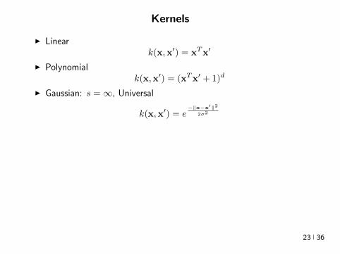
Kernels
I Lineark(xxprime) = xTxprime
I Polynomialk(xxprime) = (xTxprime + 1)d
I Gaussian s =infin Universal
k(xxprime) = eminusxminusxprime2
2σ2
I Conic combinations
k(xxprime) = α1k1(xxprime) + α2k2(xxprime)
I Elementwise products
k(xxprime) = k1(xxprime)k2(xxprime)
I Kernels on discrete sets strings graphs sequences shapes
23 36
Gaussian Kernel is Positive Definite
I Exponential
eβxTxprime = 1 + βxTxprime +
β2
2(xTy)2 +
β3
3(xTy)3 +
I For any function f Rn 7rarr R psd function k the following kernelis psd
kprime(xxprime) = f(x) (k(xxprime)) f(xprime)
Proofsumij
βiβjkprime(xixj) =
sumij
βiβjf(xi)k(xixj)f(xj) =sumij
βprimeiβprimejk(xixj) ge 0
I Gaussian Kernel
k(xxprime) = eminusxminusxprime22
2σ2
= eminusx222σ2
(e
2xT xprime2σ2
)eminusxprime222σ2 (4)
24 36
The Mathematical Naturalness of Kernel Methods
I Data X isin Rd Models isin H X 7rarr R
I Geometry in H inner product 〈middot middot〉H norm middot H (Hilbert Spaces)I Theorem All nice Hilbert spaces are generated by a symmetric
positive definite function (the kernel) k(xxprime) on X times XI if f g isin H close ie f minus gH small then f(x) g(x) close forallx isin X I Reproducing Kernel Hilbert Spaces (RKHSs) Hilbert space H
that admit a reproducing kernel ie a function k(xxprime) satisfying
(i) forallx isin X k(middotx) isin H(ii) 〈f k(middotx)〉H = f(x)
I Reproducing kernels are symmetric psdsumij
βiβjk(xixj) = 〈sumi
βik(middotxi)sumi
βik(middotxi)〉H
= sumi
βik(middotxi)2H ge 0 (5)
I (Moore-Aronsjan 1950) Symmetric psd functions arereproducing kernels for some (unique) RKHS Hk
25 36
The Mathematical Naturalness of Kernel Methods
I Data X isin Rd Models isin H X 7rarr RI Geometry in H inner product 〈middot middot〉H norm middot H (Hilbert Spaces)
I Theorem All nice Hilbert spaces are generated by a symmetricpositive definite function (the kernel) k(xxprime) on X times X
I if f g isin H close ie f minus gH small then f(x) g(x) close forallx isin X I Reproducing Kernel Hilbert Spaces (RKHSs) Hilbert space H
that admit a reproducing kernel ie a function k(xxprime) satisfying
(i) forallx isin X k(middotx) isin H(ii) 〈f k(middotx)〉H = f(x)
I Reproducing kernels are symmetric psdsumij
βiβjk(xixj) = 〈sumi
βik(middotxi)sumi
βik(middotxi)〉H
= sumi
βik(middotxi)2H ge 0 (5)
I (Moore-Aronsjan 1950) Symmetric psd functions arereproducing kernels for some (unique) RKHS Hk
25 36
The Mathematical Naturalness of Kernel Methods
I Data X isin Rd Models isin H X 7rarr RI Geometry in H inner product 〈middot middot〉H norm middot H (Hilbert Spaces)I Theorem All nice Hilbert spaces are generated by a symmetric
positive definite function (the kernel) k(xxprime) on X times XI if f g isin H close ie f minus gH small then f(x) g(x) close forallx isin X
I Reproducing Kernel Hilbert Spaces (RKHSs) Hilbert space Hthat admit a reproducing kernel ie a function k(xxprime) satisfying
(i) forallx isin X k(middotx) isin H(ii) 〈f k(middotx)〉H = f(x)
I Reproducing kernels are symmetric psdsumij
βiβjk(xixj) = 〈sumi
βik(middotxi)sumi
βik(middotxi)〉H
= sumi
βik(middotxi)2H ge 0 (5)
I (Moore-Aronsjan 1950) Symmetric psd functions arereproducing kernels for some (unique) RKHS Hk
25 36
The Mathematical Naturalness of Kernel Methods
I Data X isin Rd Models isin H X 7rarr RI Geometry in H inner product 〈middot middot〉H norm middot H (Hilbert Spaces)I Theorem All nice Hilbert spaces are generated by a symmetric
positive definite function (the kernel) k(xxprime) on X times XI if f g isin H close ie f minus gH small then f(x) g(x) close forallx isin X I Reproducing Kernel Hilbert Spaces (RKHSs) Hilbert space H
that admit a reproducing kernel ie a function k(xxprime) satisfying
(i) forallx isin X k(middotx) isin H(ii) 〈f k(middotx)〉H = f(x)
I Reproducing kernels are symmetric psdsumij
βiβjk(xixj) = 〈sumi
βik(middotxi)sumi
βik(middotxi)〉H
= sumi
βik(middotxi)2H ge 0 (5)
I (Moore-Aronsjan 1950) Symmetric psd functions arereproducing kernels for some (unique) RKHS Hk
25 36
The Mathematical Naturalness of Kernel Methods
I Data X isin Rd Models isin H X 7rarr RI Geometry in H inner product 〈middot middot〉H norm middot H (Hilbert Spaces)I Theorem All nice Hilbert spaces are generated by a symmetric
positive definite function (the kernel) k(xxprime) on X times XI if f g isin H close ie f minus gH small then f(x) g(x) close forallx isin X I Reproducing Kernel Hilbert Spaces (RKHSs) Hilbert space H
that admit a reproducing kernel ie a function k(xxprime) satisfying
(i) forallx isin X k(middotx) isin H(ii) 〈f k(middotx)〉H = f(x)
I Reproducing kernels are symmetric psdsumij
βiβjk(xixj) = 〈sumi
βik(middotxi)sumi
βik(middotxi)〉H
= sumi
βik(middotxi)2H ge 0 (5)
I (Moore-Aronsjan 1950) Symmetric psd functions arereproducing kernels for some (unique) RKHS Hk 25 36
Kernel Methods Summary
I Symm pos def function k(x z) on input domain X sub Rd
I k hArr rich Reproducing Kernel Hilbert Space (RKHS) Hk ofreal-valued functions with inner product 〈middot middot〉k and norm middot k
I Regularized Risk Minimization hArr Linear models in an implicithigh-dimensional (often infinite-dimensional) feature space
f = arg minfisinHk
1
n
nsumi=1
V (yi f(xi)) + λf2Hk xi isin Rd
I Representer Theorem f(x) =sumni=1 αik(xxi)
26 36
Shallow and Deep Function Spaces
I What does it mean to understand a function space
ndash Linear f(x) = wTxw isin Rd
ndash Polynomial f(x) = wT Ψ(x)w isin Rs
ndash RKHS balls f isin Hk fk lt γ [like vM le 1]
I Shallow nets f(x) = wTσ(Wx) (w isin RdW isin Rs)ndash For srarrinfin W sim p σ(u) = eminusiu approximates Gaussian kernel
methodsndash Theorem [Bochner 1937] One-to-one correspondence between k
and a density p such that
k(x z) = ψ(xminus z) =
intRdeminusi(xminusz)Twp(w)dw asymp 1
s
ssumj=1
eminusi(xminusz)Twj
Gaussian kernel k(x z) = eminusxminusz22
2σ2 lArrrArr p = N (0 σminus2Id)ndash Similar integral approx relates ReLU to the arc-cosine kernelndash Optimization versus Randomization
27 36
Shallow and Deep Function Spaces
I What does it mean to understand a function space
ndash Linear f(x) = wTxw isin Rd
ndash Polynomial f(x) = wT Ψ(x)w isin Rs
ndash RKHS balls f isin Hk fk lt γ [like vM le 1]
I Shallow nets f(x) = wTσ(Wx) (w isin RdW isin Rs)ndash For srarrinfin W sim p σ(u) = eminusiu approximates Gaussian kernel
methodsndash Theorem [Bochner 1937] One-to-one correspondence between k
and a density p such that
k(x z) = ψ(xminus z) =
intRdeminusi(xminusz)Twp(w)dw asymp 1
s
ssumj=1
eminusi(xminusz)Twj
Gaussian kernel k(x z) = eminusxminusz22
2σ2 lArrrArr p = N (0 σminus2Id)ndash Similar integral approx relates ReLU to the arc-cosine kernelndash Optimization versus Randomization
27 36
Shallow and Deep Function Spaces
I What does it mean to understand a function space
ndash Linear f(x) = wTxw isin Rd
ndash Polynomial f(x) = wT Ψ(x)w isin Rs
ndash RKHS balls f isin Hk fk lt γ [like vM le 1]
I Shallow nets f(x) = wTσ(Wx) (w isin RdW isin Rs)ndash For srarrinfin W sim p σ(u) = eminusiu approximates Gaussian kernel
methodsndash Theorem [Bochner 1937] One-to-one correspondence between k
and a density p such that
k(x z) = ψ(xminus z) =
intRdeminusi(xminusz)Twp(w)dw asymp 1
s
ssumj=1
eminusi(xminusz)Twj
Gaussian kernel k(x z) = eminusxminusz22
2σ2 lArrrArr p = N (0 σminus2Id)ndash Similar integral approx relates ReLU to the arc-cosine kernelndash Optimization versus Randomization
27 36
Shallow and Deep Function Spaces
I What does it mean to understand a function space
ndash Linear f(x) = wTxw isin Rd
ndash Polynomial f(x) = wT Ψ(x)w isin Rs
ndash RKHS balls f isin Hk fk lt γ [like vM le 1]
I Shallow nets f(x) = wTσ(Wx) (w isin RdW isin Rs)
ndash For srarrinfin W sim p σ(u) = eminusiu approximates Gaussian kernelmethods
ndash Theorem [Bochner 1937] One-to-one correspondence between kand a density p such that
k(x z) = ψ(xminus z) =
intRdeminusi(xminusz)Twp(w)dw asymp 1
s
ssumj=1
eminusi(xminusz)Twj
Gaussian kernel k(x z) = eminusxminusz22
2σ2 lArrrArr p = N (0 σminus2Id)ndash Similar integral approx relates ReLU to the arc-cosine kernelndash Optimization versus Randomization
27 36
Shallow and Deep Function Spaces
I What does it mean to understand a function space
ndash Linear f(x) = wTxw isin Rd
ndash Polynomial f(x) = wT Ψ(x)w isin Rs
ndash RKHS balls f isin Hk fk lt γ [like vM le 1]
I Shallow nets f(x) = wTσ(Wx) (w isin RdW isin Rs)ndash For srarrinfin W sim p σ(u) = eminusiu approximates Gaussian kernel
methodsndash Theorem [Bochner 1937] One-to-one correspondence between k
and a density p such that
k(x z) = ψ(xminus z) =
intRdeminusi(xminusz)Twp(w)dw asymp 1
s
ssumj=1
eminusi(xminusz)Twj
Gaussian kernel k(x z) = eminusxminusz22
2σ2 lArrrArr p = N (0 σminus2Id)ndash Similar integral approx relates ReLU to the arc-cosine kernelndash Optimization versus Randomization
27 36
Expressivity of Deep Nets Linear Regions
I The ReLU map f(x) = max(Wx 0)W isin Rwtimesn is piecewise linear
I A piece is a connected region (a convex polytope) of Rd with sharedsparsity pattern in activations
I (Zaslavsky 1975) Number of linear regions formed by an arrangement of
s hyperplanes in d-dimensions in general position issumd
i=0
(si
)I Composition of ReLU maps is also piecewise linear
I (Raghu et al 2017 Pascano et al 2014 Montufar 2014) Number oflinear regions grows as O(wnd) for a composition of d ReLU maps(nrarr brarr brarr b rarr b) each of width w
I (Safran and Shamir 2017)
ndash 1[x le 1] x isin Rd ε-accurate 3-layer network with O(dε) neurons but cannot be approximated with
accuracy higher than O(1d4) using 2-layer networks unless width is exponential in d
28 36
Expressivity of Deep Nets Linear Regions
I The ReLU map f(x) = max(Wx 0)W isin Rwtimesn is piecewise linear
I A piece is a connected region (a convex polytope) of Rd with sharedsparsity pattern in activations
I (Zaslavsky 1975) Number of linear regions formed by an arrangement of
s hyperplanes in d-dimensions in general position issumd
i=0
(si
)I Composition of ReLU maps is also piecewise linear
I (Raghu et al 2017 Pascano et al 2014 Montufar 2014) Number oflinear regions grows as O(wnd) for a composition of d ReLU maps(nrarr brarr brarr b rarr b) each of width w
I (Safran and Shamir 2017)
ndash 1[x le 1] x isin Rd ε-accurate 3-layer network with O(dε) neurons but cannot be approximated with
accuracy higher than O(1d4) using 2-layer networks unless width is exponential in d
28 36
Expressivity of Deep Nets Linear Regions
I The ReLU map f(x) = max(Wx 0)W isin Rwtimesn is piecewise linear
I A piece is a connected region (a convex polytope) of Rd with sharedsparsity pattern in activations
I (Zaslavsky 1975) Number of linear regions formed by an arrangement of
s hyperplanes in d-dimensions in general position issumd
i=0
(si
)
I Composition of ReLU maps is also piecewise linear
I (Raghu et al 2017 Pascano et al 2014 Montufar 2014) Number oflinear regions grows as O(wnd) for a composition of d ReLU maps(nrarr brarr brarr b rarr b) each of width w
I (Safran and Shamir 2017)
ndash 1[x le 1] x isin Rd ε-accurate 3-layer network with O(dε) neurons but cannot be approximated with
accuracy higher than O(1d4) using 2-layer networks unless width is exponential in d
28 36
Expressivity of Deep Nets Linear Regions
I The ReLU map f(x) = max(Wx 0)W isin Rwtimesn is piecewise linear
I A piece is a connected region (a convex polytope) of Rd with sharedsparsity pattern in activations
I (Zaslavsky 1975) Number of linear regions formed by an arrangement of
s hyperplanes in d-dimensions in general position issumd
i=0
(si
)I Composition of ReLU maps is also piecewise linear
I (Raghu et al 2017 Pascano et al 2014 Montufar 2014) Number oflinear regions grows as O(wnd) for a composition of d ReLU maps(nrarr brarr brarr b rarr b) each of width w
I (Safran and Shamir 2017)
ndash 1[x le 1] x isin Rd ε-accurate 3-layer network with O(dε) neurons but cannot be approximated with
accuracy higher than O(1d4) using 2-layer networks unless width is exponential in d28 36
Expressivity of Deep Nets Trajectory Length
I (Raghu et al 2017) Trajectory Length (ldquogeneralized operator normrdquo)How much is a curve in the input space stretched by a layer in thenetwork
29 36
Expressivity of Deep Nets Trajectory Length
I (Raghu et al 2017) Trajectory Length (ldquogeneralized operator normrdquo)How much is a curve in the input space stretched by a layer in thenetwork
29 36
Expressivity and Generalization
I Expressiveness equiv capacity to fit random noise =rArr susceptibility tooverfitting (VC dimension Rademacher Complexity)
I Zhang et al 2017 Famous CNNs easily fit random labels
ndash Over-parameterized (n=12M psim 60M) but structuredndash Domain-knowledge baked in does not constraint expressiveness
I CNNs tend to generalize even without regularization (explicit and implicit)
I For linear regression SGD returns minimum norm solution
30 36
Expressivity and Generalization
I Expressiveness equiv capacity to fit random noise =rArr susceptibility tooverfitting (VC dimension Rademacher Complexity)
I Zhang et al 2017 Famous CNNs easily fit random labels
ndash Over-parameterized (n=12M psim 60M) but structuredndash Domain-knowledge baked in does not constraint expressiveness
I CNNs tend to generalize even without regularization (explicit and implicit)
I For linear regression SGD returns minimum norm solution
30 36
Expressivity and Generalization
I Expressiveness equiv capacity to fit random noise =rArr susceptibility tooverfitting (VC dimension Rademacher Complexity)
I Zhang et al 2017 Famous CNNs easily fit random labels
ndash Over-parameterized (n=12M psim 60M) but structuredndash Domain-knowledge baked in does not constraint expressiveness
I CNNs tend to generalize even without regularization (explicit and implicit)
I For linear regression SGD returns minimum norm solution
30 36
Optimization Landscape Symmetry and Saddle Points
I Folklore lots of equivalent good local minI Classification of critical points based on Hessian spectrumI Permutation and Scaling symmetries
I Thm [Lee et al 2016 Anadkumar Ge] For the short-step gradientmethod the basin of attraction of strict saddle points (atleast onenegative eigenvalue) has measure zero
31 36
Optimization Landscape Symmetry and Saddle Points
I Folklore lots of equivalent good local minI Classification of critical points based on Hessian spectrumI Permutation and Scaling symmetries
I Thm [Lee et al 2016 Anadkumar Ge] For the short-step gradientmethod the basin of attraction of strict saddle points (atleast onenegative eigenvalue) has measure zero
31 36
Optimization Landscape Symmetry and Saddle Points
I Folklore lots of equivalent good local minI Classification of critical points based on Hessian spectrumI Permutation and Scaling symmetries
I Thm [Lee et al 2016 Anadkumar Ge] For the short-step gradientmethod the basin of attraction of strict saddle points (atleast onenegative eigenvalue) has measure zero
31 36
Optimization Landscape Sharp Minima and Stability
Keskar et al 2017 On large-batch training for DL Generalization Gap and Sharp Minima
32 36
Deep Learning Computational Graphs TensorFlow
tensorfloworg
I Tensors-in Tensors-out
I Evergrowing list of Tensor-Ops (PythonC++)
f(xw)
[partf
partx
]T v
[partf
partw
]T v
I Automatic Differentiation Reverse mode
partxL
partxi=sumirarrj
partxL
partxj
partxj
partxi
33 36
Computational Graphs and TensorFlow
tensorfloworg
I SGD with minibatches
wk+1 = wk minus ηlsumi=1
partli
partw
∣∣∣wt
I Model Parallelism Assign independent paths tothreads GPUs
I Data Parallelism create Graph replicas on differentmachines
I Mobile TensorFlow
34 36
Computational Graphs and TensorFlow
tensorfloworg
35 36
Computational Graphs and TensorFlow
tensorfloworg
35 36
Computational Graphs and TensorFlow
tensorfloworg
35 36
Challenges and Opportunities
I Lots of fascinating unsolved problems
I Can you win Imagenet with Convex optimization
I Tools from polynomial optimization (global optimization deep-RL)
I Supervised to Semi-supervised to Unsupervised Learning
I Compact efficient real-time models (eliminateover-parametrization) for new form factors
I Exciting emerging world of Robotics Wearable ComputersIntelligent home devices Personal digital assistants
Google Internship Program
36 36
- anm0
- fdrm0
- fdrm5

Kernels
I Lineark(xxprime) = xTxprime
I Polynomialk(xxprime) = (xTxprime + 1)d
I Gaussian s =infin Universal
k(xxprime) = eminusxminusxprime2
2σ2
I Conic combinations
k(xxprime) = α1k1(xxprime) + α2k2(xxprime)
I Elementwise products
k(xxprime) = k1(xxprime)k2(xxprime)
I Kernels on discrete sets strings graphs sequences shapes
23 36
Kernels
I Lineark(xxprime) = xTxprime
I Polynomialk(xxprime) = (xTxprime + 1)d
I Gaussian s =infin Universal
k(xxprime) = eminusxminusxprime2
2σ2
I Conic combinations
k(xxprime) = α1k1(xxprime) + α2k2(xxprime)
I Elementwise products
k(xxprime) = k1(xxprime)k2(xxprime)
I Kernels on discrete sets strings graphs sequences shapes
23 36
Gaussian Kernel is Positive Definite
I Exponential
eβxTxprime = 1 + βxTxprime +
β2
2(xTy)2 +
β3
3(xTy)3 +
I For any function f Rn 7rarr R psd function k the following kernelis psd
kprime(xxprime) = f(x) (k(xxprime)) f(xprime)
Proofsumij
βiβjkprime(xixj) =
sumij
βiβjf(xi)k(xixj)f(xj) =sumij
βprimeiβprimejk(xixj) ge 0
I Gaussian Kernel
k(xxprime) = eminusxminusxprime22
2σ2
= eminusx222σ2
(e
2xT xprime2σ2
)eminusxprime222σ2 (4)
24 36
The Mathematical Naturalness of Kernel Methods
I Data X isin Rd Models isin H X 7rarr R
I Geometry in H inner product 〈middot middot〉H norm middot H (Hilbert Spaces)I Theorem All nice Hilbert spaces are generated by a symmetric
positive definite function (the kernel) k(xxprime) on X times XI if f g isin H close ie f minus gH small then f(x) g(x) close forallx isin X I Reproducing Kernel Hilbert Spaces (RKHSs) Hilbert space H
that admit a reproducing kernel ie a function k(xxprime) satisfying
(i) forallx isin X k(middotx) isin H(ii) 〈f k(middotx)〉H = f(x)
I Reproducing kernels are symmetric psdsumij
βiβjk(xixj) = 〈sumi
βik(middotxi)sumi
βik(middotxi)〉H
= sumi
βik(middotxi)2H ge 0 (5)
I (Moore-Aronsjan 1950) Symmetric psd functions arereproducing kernels for some (unique) RKHS Hk
25 36
The Mathematical Naturalness of Kernel Methods
I Data X isin Rd Models isin H X 7rarr RI Geometry in H inner product 〈middot middot〉H norm middot H (Hilbert Spaces)
I Theorem All nice Hilbert spaces are generated by a symmetricpositive definite function (the kernel) k(xxprime) on X times X
I if f g isin H close ie f minus gH small then f(x) g(x) close forallx isin X I Reproducing Kernel Hilbert Spaces (RKHSs) Hilbert space H
that admit a reproducing kernel ie a function k(xxprime) satisfying
(i) forallx isin X k(middotx) isin H(ii) 〈f k(middotx)〉H = f(x)
I Reproducing kernels are symmetric psdsumij
βiβjk(xixj) = 〈sumi
βik(middotxi)sumi
βik(middotxi)〉H
= sumi
βik(middotxi)2H ge 0 (5)
I (Moore-Aronsjan 1950) Symmetric psd functions arereproducing kernels for some (unique) RKHS Hk
25 36
The Mathematical Naturalness of Kernel Methods
I Data X isin Rd Models isin H X 7rarr RI Geometry in H inner product 〈middot middot〉H norm middot H (Hilbert Spaces)I Theorem All nice Hilbert spaces are generated by a symmetric
positive definite function (the kernel) k(xxprime) on X times XI if f g isin H close ie f minus gH small then f(x) g(x) close forallx isin X
I Reproducing Kernel Hilbert Spaces (RKHSs) Hilbert space Hthat admit a reproducing kernel ie a function k(xxprime) satisfying
(i) forallx isin X k(middotx) isin H(ii) 〈f k(middotx)〉H = f(x)
I Reproducing kernels are symmetric psdsumij
βiβjk(xixj) = 〈sumi
βik(middotxi)sumi
βik(middotxi)〉H
= sumi
βik(middotxi)2H ge 0 (5)
I (Moore-Aronsjan 1950) Symmetric psd functions arereproducing kernels for some (unique) RKHS Hk
25 36
The Mathematical Naturalness of Kernel Methods
I Data X isin Rd Models isin H X 7rarr RI Geometry in H inner product 〈middot middot〉H norm middot H (Hilbert Spaces)I Theorem All nice Hilbert spaces are generated by a symmetric
positive definite function (the kernel) k(xxprime) on X times XI if f g isin H close ie f minus gH small then f(x) g(x) close forallx isin X I Reproducing Kernel Hilbert Spaces (RKHSs) Hilbert space H
that admit a reproducing kernel ie a function k(xxprime) satisfying
(i) forallx isin X k(middotx) isin H(ii) 〈f k(middotx)〉H = f(x)
I Reproducing kernels are symmetric psdsumij
βiβjk(xixj) = 〈sumi
βik(middotxi)sumi
βik(middotxi)〉H
= sumi
βik(middotxi)2H ge 0 (5)
I (Moore-Aronsjan 1950) Symmetric psd functions arereproducing kernels for some (unique) RKHS Hk
25 36
The Mathematical Naturalness of Kernel Methods
I Data X isin Rd Models isin H X 7rarr RI Geometry in H inner product 〈middot middot〉H norm middot H (Hilbert Spaces)I Theorem All nice Hilbert spaces are generated by a symmetric
positive definite function (the kernel) k(xxprime) on X times XI if f g isin H close ie f minus gH small then f(x) g(x) close forallx isin X I Reproducing Kernel Hilbert Spaces (RKHSs) Hilbert space H
that admit a reproducing kernel ie a function k(xxprime) satisfying
(i) forallx isin X k(middotx) isin H(ii) 〈f k(middotx)〉H = f(x)
I Reproducing kernels are symmetric psdsumij
βiβjk(xixj) = 〈sumi
βik(middotxi)sumi
βik(middotxi)〉H
= sumi
βik(middotxi)2H ge 0 (5)
I (Moore-Aronsjan 1950) Symmetric psd functions arereproducing kernels for some (unique) RKHS Hk 25 36
Kernel Methods Summary
I Symm pos def function k(x z) on input domain X sub Rd
I k hArr rich Reproducing Kernel Hilbert Space (RKHS) Hk ofreal-valued functions with inner product 〈middot middot〉k and norm middot k
I Regularized Risk Minimization hArr Linear models in an implicithigh-dimensional (often infinite-dimensional) feature space
f = arg minfisinHk
1
n
nsumi=1
V (yi f(xi)) + λf2Hk xi isin Rd
I Representer Theorem f(x) =sumni=1 αik(xxi)
26 36
Shallow and Deep Function Spaces
I What does it mean to understand a function space
ndash Linear f(x) = wTxw isin Rd
ndash Polynomial f(x) = wT Ψ(x)w isin Rs
ndash RKHS balls f isin Hk fk lt γ [like vM le 1]
I Shallow nets f(x) = wTσ(Wx) (w isin RdW isin Rs)ndash For srarrinfin W sim p σ(u) = eminusiu approximates Gaussian kernel
methodsndash Theorem [Bochner 1937] One-to-one correspondence between k
and a density p such that
k(x z) = ψ(xminus z) =
intRdeminusi(xminusz)Twp(w)dw asymp 1
s
ssumj=1
eminusi(xminusz)Twj
Gaussian kernel k(x z) = eminusxminusz22
2σ2 lArrrArr p = N (0 σminus2Id)ndash Similar integral approx relates ReLU to the arc-cosine kernelndash Optimization versus Randomization
27 36
Shallow and Deep Function Spaces
I What does it mean to understand a function space
ndash Linear f(x) = wTxw isin Rd
ndash Polynomial f(x) = wT Ψ(x)w isin Rs
ndash RKHS balls f isin Hk fk lt γ [like vM le 1]
I Shallow nets f(x) = wTσ(Wx) (w isin RdW isin Rs)ndash For srarrinfin W sim p σ(u) = eminusiu approximates Gaussian kernel
methodsndash Theorem [Bochner 1937] One-to-one correspondence between k
and a density p such that
k(x z) = ψ(xminus z) =
intRdeminusi(xminusz)Twp(w)dw asymp 1
s
ssumj=1
eminusi(xminusz)Twj
Gaussian kernel k(x z) = eminusxminusz22
2σ2 lArrrArr p = N (0 σminus2Id)ndash Similar integral approx relates ReLU to the arc-cosine kernelndash Optimization versus Randomization
27 36
Shallow and Deep Function Spaces
I What does it mean to understand a function space
ndash Linear f(x) = wTxw isin Rd
ndash Polynomial f(x) = wT Ψ(x)w isin Rs
ndash RKHS balls f isin Hk fk lt γ [like vM le 1]
I Shallow nets f(x) = wTσ(Wx) (w isin RdW isin Rs)ndash For srarrinfin W sim p σ(u) = eminusiu approximates Gaussian kernel
methodsndash Theorem [Bochner 1937] One-to-one correspondence between k
and a density p such that
k(x z) = ψ(xminus z) =
intRdeminusi(xminusz)Twp(w)dw asymp 1
s
ssumj=1
eminusi(xminusz)Twj
Gaussian kernel k(x z) = eminusxminusz22
2σ2 lArrrArr p = N (0 σminus2Id)ndash Similar integral approx relates ReLU to the arc-cosine kernelndash Optimization versus Randomization
27 36
Shallow and Deep Function Spaces
I What does it mean to understand a function space
ndash Linear f(x) = wTxw isin Rd
ndash Polynomial f(x) = wT Ψ(x)w isin Rs
ndash RKHS balls f isin Hk fk lt γ [like vM le 1]
I Shallow nets f(x) = wTσ(Wx) (w isin RdW isin Rs)
ndash For srarrinfin W sim p σ(u) = eminusiu approximates Gaussian kernelmethods
ndash Theorem [Bochner 1937] One-to-one correspondence between kand a density p such that
k(x z) = ψ(xminus z) =
intRdeminusi(xminusz)Twp(w)dw asymp 1
s
ssumj=1
eminusi(xminusz)Twj
Gaussian kernel k(x z) = eminusxminusz22
2σ2 lArrrArr p = N (0 σminus2Id)ndash Similar integral approx relates ReLU to the arc-cosine kernelndash Optimization versus Randomization
27 36
Shallow and Deep Function Spaces
I What does it mean to understand a function space
ndash Linear f(x) = wTxw isin Rd
ndash Polynomial f(x) = wT Ψ(x)w isin Rs
ndash RKHS balls f isin Hk fk lt γ [like vM le 1]
I Shallow nets f(x) = wTσ(Wx) (w isin RdW isin Rs)ndash For srarrinfin W sim p σ(u) = eminusiu approximates Gaussian kernel
methodsndash Theorem [Bochner 1937] One-to-one correspondence between k
and a density p such that
k(x z) = ψ(xminus z) =
intRdeminusi(xminusz)Twp(w)dw asymp 1
s
ssumj=1
eminusi(xminusz)Twj
Gaussian kernel k(x z) = eminusxminusz22
2σ2 lArrrArr p = N (0 σminus2Id)ndash Similar integral approx relates ReLU to the arc-cosine kernelndash Optimization versus Randomization
27 36
Expressivity of Deep Nets Linear Regions
I The ReLU map f(x) = max(Wx 0)W isin Rwtimesn is piecewise linear
I A piece is a connected region (a convex polytope) of Rd with sharedsparsity pattern in activations
I (Zaslavsky 1975) Number of linear regions formed by an arrangement of
s hyperplanes in d-dimensions in general position issumd
i=0
(si
)I Composition of ReLU maps is also piecewise linear
I (Raghu et al 2017 Pascano et al 2014 Montufar 2014) Number oflinear regions grows as O(wnd) for a composition of d ReLU maps(nrarr brarr brarr b rarr b) each of width w
I (Safran and Shamir 2017)
ndash 1[x le 1] x isin Rd ε-accurate 3-layer network with O(dε) neurons but cannot be approximated with
accuracy higher than O(1d4) using 2-layer networks unless width is exponential in d
28 36
Expressivity of Deep Nets Linear Regions
I The ReLU map f(x) = max(Wx 0)W isin Rwtimesn is piecewise linear
I A piece is a connected region (a convex polytope) of Rd with sharedsparsity pattern in activations
I (Zaslavsky 1975) Number of linear regions formed by an arrangement of
s hyperplanes in d-dimensions in general position issumd
i=0
(si
)I Composition of ReLU maps is also piecewise linear
I (Raghu et al 2017 Pascano et al 2014 Montufar 2014) Number oflinear regions grows as O(wnd) for a composition of d ReLU maps(nrarr brarr brarr b rarr b) each of width w
I (Safran and Shamir 2017)
ndash 1[x le 1] x isin Rd ε-accurate 3-layer network with O(dε) neurons but cannot be approximated with
accuracy higher than O(1d4) using 2-layer networks unless width is exponential in d
28 36
Expressivity of Deep Nets Linear Regions
I The ReLU map f(x) = max(Wx 0)W isin Rwtimesn is piecewise linear
I A piece is a connected region (a convex polytope) of Rd with sharedsparsity pattern in activations
I (Zaslavsky 1975) Number of linear regions formed by an arrangement of
s hyperplanes in d-dimensions in general position issumd
i=0
(si
)
I Composition of ReLU maps is also piecewise linear
I (Raghu et al 2017 Pascano et al 2014 Montufar 2014) Number oflinear regions grows as O(wnd) for a composition of d ReLU maps(nrarr brarr brarr b rarr b) each of width w
I (Safran and Shamir 2017)
ndash 1[x le 1] x isin Rd ε-accurate 3-layer network with O(dε) neurons but cannot be approximated with
accuracy higher than O(1d4) using 2-layer networks unless width is exponential in d
28 36
Expressivity of Deep Nets Linear Regions
I The ReLU map f(x) = max(Wx 0)W isin Rwtimesn is piecewise linear
I A piece is a connected region (a convex polytope) of Rd with sharedsparsity pattern in activations
I (Zaslavsky 1975) Number of linear regions formed by an arrangement of
s hyperplanes in d-dimensions in general position issumd
i=0
(si
)I Composition of ReLU maps is also piecewise linear
I (Raghu et al 2017 Pascano et al 2014 Montufar 2014) Number oflinear regions grows as O(wnd) for a composition of d ReLU maps(nrarr brarr brarr b rarr b) each of width w
I (Safran and Shamir 2017)
ndash 1[x le 1] x isin Rd ε-accurate 3-layer network with O(dε) neurons but cannot be approximated with
accuracy higher than O(1d4) using 2-layer networks unless width is exponential in d28 36
Expressivity of Deep Nets Trajectory Length
I (Raghu et al 2017) Trajectory Length (ldquogeneralized operator normrdquo)How much is a curve in the input space stretched by a layer in thenetwork
29 36
Expressivity of Deep Nets Trajectory Length
I (Raghu et al 2017) Trajectory Length (ldquogeneralized operator normrdquo)How much is a curve in the input space stretched by a layer in thenetwork
29 36
Expressivity and Generalization
I Expressiveness equiv capacity to fit random noise =rArr susceptibility tooverfitting (VC dimension Rademacher Complexity)
I Zhang et al 2017 Famous CNNs easily fit random labels
ndash Over-parameterized (n=12M psim 60M) but structuredndash Domain-knowledge baked in does not constraint expressiveness
I CNNs tend to generalize even without regularization (explicit and implicit)
I For linear regression SGD returns minimum norm solution
30 36
Expressivity and Generalization
I Expressiveness equiv capacity to fit random noise =rArr susceptibility tooverfitting (VC dimension Rademacher Complexity)
I Zhang et al 2017 Famous CNNs easily fit random labels
ndash Over-parameterized (n=12M psim 60M) but structuredndash Domain-knowledge baked in does not constraint expressiveness
I CNNs tend to generalize even without regularization (explicit and implicit)
I For linear regression SGD returns minimum norm solution
30 36
Expressivity and Generalization
I Expressiveness equiv capacity to fit random noise =rArr susceptibility tooverfitting (VC dimension Rademacher Complexity)
I Zhang et al 2017 Famous CNNs easily fit random labels
ndash Over-parameterized (n=12M psim 60M) but structuredndash Domain-knowledge baked in does not constraint expressiveness
I CNNs tend to generalize even without regularization (explicit and implicit)
I For linear regression SGD returns minimum norm solution
30 36
Optimization Landscape Symmetry and Saddle Points
I Folklore lots of equivalent good local minI Classification of critical points based on Hessian spectrumI Permutation and Scaling symmetries
I Thm [Lee et al 2016 Anadkumar Ge] For the short-step gradientmethod the basin of attraction of strict saddle points (atleast onenegative eigenvalue) has measure zero
31 36
Optimization Landscape Symmetry and Saddle Points
I Folklore lots of equivalent good local minI Classification of critical points based on Hessian spectrumI Permutation and Scaling symmetries
I Thm [Lee et al 2016 Anadkumar Ge] For the short-step gradientmethod the basin of attraction of strict saddle points (atleast onenegative eigenvalue) has measure zero
31 36
Optimization Landscape Symmetry and Saddle Points
I Folklore lots of equivalent good local minI Classification of critical points based on Hessian spectrumI Permutation and Scaling symmetries
I Thm [Lee et al 2016 Anadkumar Ge] For the short-step gradientmethod the basin of attraction of strict saddle points (atleast onenegative eigenvalue) has measure zero
31 36
Optimization Landscape Sharp Minima and Stability
Keskar et al 2017 On large-batch training for DL Generalization Gap and Sharp Minima
32 36
Deep Learning Computational Graphs TensorFlow
tensorfloworg
I Tensors-in Tensors-out
I Evergrowing list of Tensor-Ops (PythonC++)
f(xw)
[partf
partx
]T v
[partf
partw
]T v
I Automatic Differentiation Reverse mode
partxL
partxi=sumirarrj
partxL
partxj
partxj
partxi
33 36
Computational Graphs and TensorFlow
tensorfloworg
I SGD with minibatches
wk+1 = wk minus ηlsumi=1
partli
partw
∣∣∣wt
I Model Parallelism Assign independent paths tothreads GPUs
I Data Parallelism create Graph replicas on differentmachines
I Mobile TensorFlow
34 36
Computational Graphs and TensorFlow
tensorfloworg
35 36
Computational Graphs and TensorFlow
tensorfloworg
35 36
Computational Graphs and TensorFlow
tensorfloworg
35 36
Challenges and Opportunities
I Lots of fascinating unsolved problems
I Can you win Imagenet with Convex optimization
I Tools from polynomial optimization (global optimization deep-RL)
I Supervised to Semi-supervised to Unsupervised Learning
I Compact efficient real-time models (eliminateover-parametrization) for new form factors
I Exciting emerging world of Robotics Wearable ComputersIntelligent home devices Personal digital assistants
Google Internship Program
36 36
- anm0
- fdrm0
- fdrm5

Kernels
I Lineark(xxprime) = xTxprime
I Polynomialk(xxprime) = (xTxprime + 1)d
I Gaussian s =infin Universal
k(xxprime) = eminusxminusxprime2
2σ2
I Conic combinations
k(xxprime) = α1k1(xxprime) + α2k2(xxprime)
I Elementwise products
k(xxprime) = k1(xxprime)k2(xxprime)
I Kernels on discrete sets strings graphs sequences shapes
23 36
Gaussian Kernel is Positive Definite
I Exponential
eβxTxprime = 1 + βxTxprime +
β2
2(xTy)2 +
β3
3(xTy)3 +
I For any function f Rn 7rarr R psd function k the following kernelis psd
kprime(xxprime) = f(x) (k(xxprime)) f(xprime)
Proofsumij
βiβjkprime(xixj) =
sumij
βiβjf(xi)k(xixj)f(xj) =sumij
βprimeiβprimejk(xixj) ge 0
I Gaussian Kernel
k(xxprime) = eminusxminusxprime22
2σ2
= eminusx222σ2
(e
2xT xprime2σ2
)eminusxprime222σ2 (4)
24 36
The Mathematical Naturalness of Kernel Methods
I Data X isin Rd Models isin H X 7rarr R
I Geometry in H inner product 〈middot middot〉H norm middot H (Hilbert Spaces)I Theorem All nice Hilbert spaces are generated by a symmetric
positive definite function (the kernel) k(xxprime) on X times XI if f g isin H close ie f minus gH small then f(x) g(x) close forallx isin X I Reproducing Kernel Hilbert Spaces (RKHSs) Hilbert space H
that admit a reproducing kernel ie a function k(xxprime) satisfying
(i) forallx isin X k(middotx) isin H(ii) 〈f k(middotx)〉H = f(x)
I Reproducing kernels are symmetric psdsumij
βiβjk(xixj) = 〈sumi
βik(middotxi)sumi
βik(middotxi)〉H
= sumi
βik(middotxi)2H ge 0 (5)
I (Moore-Aronsjan 1950) Symmetric psd functions arereproducing kernels for some (unique) RKHS Hk
25 36
The Mathematical Naturalness of Kernel Methods
I Data X isin Rd Models isin H X 7rarr RI Geometry in H inner product 〈middot middot〉H norm middot H (Hilbert Spaces)
I Theorem All nice Hilbert spaces are generated by a symmetricpositive definite function (the kernel) k(xxprime) on X times X
I if f g isin H close ie f minus gH small then f(x) g(x) close forallx isin X I Reproducing Kernel Hilbert Spaces (RKHSs) Hilbert space H
that admit a reproducing kernel ie a function k(xxprime) satisfying
(i) forallx isin X k(middotx) isin H(ii) 〈f k(middotx)〉H = f(x)
I Reproducing kernels are symmetric psdsumij
βiβjk(xixj) = 〈sumi
βik(middotxi)sumi
βik(middotxi)〉H
= sumi
βik(middotxi)2H ge 0 (5)
I (Moore-Aronsjan 1950) Symmetric psd functions arereproducing kernels for some (unique) RKHS Hk
25 36
The Mathematical Naturalness of Kernel Methods
I Data X isin Rd Models isin H X 7rarr RI Geometry in H inner product 〈middot middot〉H norm middot H (Hilbert Spaces)I Theorem All nice Hilbert spaces are generated by a symmetric
positive definite function (the kernel) k(xxprime) on X times XI if f g isin H close ie f minus gH small then f(x) g(x) close forallx isin X
I Reproducing Kernel Hilbert Spaces (RKHSs) Hilbert space Hthat admit a reproducing kernel ie a function k(xxprime) satisfying
(i) forallx isin X k(middotx) isin H(ii) 〈f k(middotx)〉H = f(x)
I Reproducing kernels are symmetric psdsumij
βiβjk(xixj) = 〈sumi
βik(middotxi)sumi
βik(middotxi)〉H
= sumi
βik(middotxi)2H ge 0 (5)
I (Moore-Aronsjan 1950) Symmetric psd functions arereproducing kernels for some (unique) RKHS Hk
25 36
The Mathematical Naturalness of Kernel Methods
I Data X isin Rd Models isin H X 7rarr RI Geometry in H inner product 〈middot middot〉H norm middot H (Hilbert Spaces)I Theorem All nice Hilbert spaces are generated by a symmetric
positive definite function (the kernel) k(xxprime) on X times XI if f g isin H close ie f minus gH small then f(x) g(x) close forallx isin X I Reproducing Kernel Hilbert Spaces (RKHSs) Hilbert space H
that admit a reproducing kernel ie a function k(xxprime) satisfying
(i) forallx isin X k(middotx) isin H(ii) 〈f k(middotx)〉H = f(x)
I Reproducing kernels are symmetric psdsumij
βiβjk(xixj) = 〈sumi
βik(middotxi)sumi
βik(middotxi)〉H
= sumi
βik(middotxi)2H ge 0 (5)
I (Moore-Aronsjan 1950) Symmetric psd functions arereproducing kernels for some (unique) RKHS Hk
25 36
The Mathematical Naturalness of Kernel Methods
I Data X isin Rd Models isin H X 7rarr RI Geometry in H inner product 〈middot middot〉H norm middot H (Hilbert Spaces)I Theorem All nice Hilbert spaces are generated by a symmetric
positive definite function (the kernel) k(xxprime) on X times XI if f g isin H close ie f minus gH small then f(x) g(x) close forallx isin X I Reproducing Kernel Hilbert Spaces (RKHSs) Hilbert space H
that admit a reproducing kernel ie a function k(xxprime) satisfying
(i) forallx isin X k(middotx) isin H(ii) 〈f k(middotx)〉H = f(x)
I Reproducing kernels are symmetric psdsumij
βiβjk(xixj) = 〈sumi
βik(middotxi)sumi
βik(middotxi)〉H
= sumi
βik(middotxi)2H ge 0 (5)
I (Moore-Aronsjan 1950) Symmetric psd functions arereproducing kernels for some (unique) RKHS Hk 25 36
Kernel Methods Summary
I Symm pos def function k(x z) on input domain X sub Rd
I k hArr rich Reproducing Kernel Hilbert Space (RKHS) Hk ofreal-valued functions with inner product 〈middot middot〉k and norm middot k
I Regularized Risk Minimization hArr Linear models in an implicithigh-dimensional (often infinite-dimensional) feature space
f = arg minfisinHk
1
n
nsumi=1
V (yi f(xi)) + λf2Hk xi isin Rd
I Representer Theorem f(x) =sumni=1 αik(xxi)
26 36
Shallow and Deep Function Spaces
I What does it mean to understand a function space
ndash Linear f(x) = wTxw isin Rd
ndash Polynomial f(x) = wT Ψ(x)w isin Rs
ndash RKHS balls f isin Hk fk lt γ [like vM le 1]
I Shallow nets f(x) = wTσ(Wx) (w isin RdW isin Rs)ndash For srarrinfin W sim p σ(u) = eminusiu approximates Gaussian kernel
methodsndash Theorem [Bochner 1937] One-to-one correspondence between k
and a density p such that
k(x z) = ψ(xminus z) =
intRdeminusi(xminusz)Twp(w)dw asymp 1
s
ssumj=1
eminusi(xminusz)Twj
Gaussian kernel k(x z) = eminusxminusz22
2σ2 lArrrArr p = N (0 σminus2Id)ndash Similar integral approx relates ReLU to the arc-cosine kernelndash Optimization versus Randomization
27 36
Shallow and Deep Function Spaces
I What does it mean to understand a function space
ndash Linear f(x) = wTxw isin Rd
ndash Polynomial f(x) = wT Ψ(x)w isin Rs
ndash RKHS balls f isin Hk fk lt γ [like vM le 1]
I Shallow nets f(x) = wTσ(Wx) (w isin RdW isin Rs)ndash For srarrinfin W sim p σ(u) = eminusiu approximates Gaussian kernel
methodsndash Theorem [Bochner 1937] One-to-one correspondence between k
and a density p such that
k(x z) = ψ(xminus z) =
intRdeminusi(xminusz)Twp(w)dw asymp 1
s
ssumj=1
eminusi(xminusz)Twj
Gaussian kernel k(x z) = eminusxminusz22
2σ2 lArrrArr p = N (0 σminus2Id)ndash Similar integral approx relates ReLU to the arc-cosine kernelndash Optimization versus Randomization
27 36
Shallow and Deep Function Spaces
I What does it mean to understand a function space
ndash Linear f(x) = wTxw isin Rd
ndash Polynomial f(x) = wT Ψ(x)w isin Rs
ndash RKHS balls f isin Hk fk lt γ [like vM le 1]
I Shallow nets f(x) = wTσ(Wx) (w isin RdW isin Rs)ndash For srarrinfin W sim p σ(u) = eminusiu approximates Gaussian kernel
methodsndash Theorem [Bochner 1937] One-to-one correspondence between k
and a density p such that
k(x z) = ψ(xminus z) =
intRdeminusi(xminusz)Twp(w)dw asymp 1
s
ssumj=1
eminusi(xminusz)Twj
Gaussian kernel k(x z) = eminusxminusz22
2σ2 lArrrArr p = N (0 σminus2Id)ndash Similar integral approx relates ReLU to the arc-cosine kernelndash Optimization versus Randomization
27 36
Shallow and Deep Function Spaces
I What does it mean to understand a function space
ndash Linear f(x) = wTxw isin Rd
ndash Polynomial f(x) = wT Ψ(x)w isin Rs
ndash RKHS balls f isin Hk fk lt γ [like vM le 1]
I Shallow nets f(x) = wTσ(Wx) (w isin RdW isin Rs)
ndash For srarrinfin W sim p σ(u) = eminusiu approximates Gaussian kernelmethods
ndash Theorem [Bochner 1937] One-to-one correspondence between kand a density p such that
k(x z) = ψ(xminus z) =
intRdeminusi(xminusz)Twp(w)dw asymp 1
s
ssumj=1
eminusi(xminusz)Twj
Gaussian kernel k(x z) = eminusxminusz22
2σ2 lArrrArr p = N (0 σminus2Id)ndash Similar integral approx relates ReLU to the arc-cosine kernelndash Optimization versus Randomization
27 36
Shallow and Deep Function Spaces
I What does it mean to understand a function space
ndash Linear f(x) = wTxw isin Rd
ndash Polynomial f(x) = wT Ψ(x)w isin Rs
ndash RKHS balls f isin Hk fk lt γ [like vM le 1]
I Shallow nets f(x) = wTσ(Wx) (w isin RdW isin Rs)ndash For srarrinfin W sim p σ(u) = eminusiu approximates Gaussian kernel
methodsndash Theorem [Bochner 1937] One-to-one correspondence between k
and a density p such that
k(x z) = ψ(xminus z) =
intRdeminusi(xminusz)Twp(w)dw asymp 1
s
ssumj=1
eminusi(xminusz)Twj
Gaussian kernel k(x z) = eminusxminusz22
2σ2 lArrrArr p = N (0 σminus2Id)ndash Similar integral approx relates ReLU to the arc-cosine kernelndash Optimization versus Randomization
27 36
Expressivity of Deep Nets Linear Regions
I The ReLU map f(x) = max(Wx 0)W isin Rwtimesn is piecewise linear
I A piece is a connected region (a convex polytope) of Rd with sharedsparsity pattern in activations
I (Zaslavsky 1975) Number of linear regions formed by an arrangement of
s hyperplanes in d-dimensions in general position issumd
i=0
(si
)I Composition of ReLU maps is also piecewise linear
I (Raghu et al 2017 Pascano et al 2014 Montufar 2014) Number oflinear regions grows as O(wnd) for a composition of d ReLU maps(nrarr brarr brarr b rarr b) each of width w
I (Safran and Shamir 2017)
ndash 1[x le 1] x isin Rd ε-accurate 3-layer network with O(dε) neurons but cannot be approximated with
accuracy higher than O(1d4) using 2-layer networks unless width is exponential in d
28 36
Expressivity of Deep Nets Linear Regions
I The ReLU map f(x) = max(Wx 0)W isin Rwtimesn is piecewise linear
I A piece is a connected region (a convex polytope) of Rd with sharedsparsity pattern in activations
I (Zaslavsky 1975) Number of linear regions formed by an arrangement of
s hyperplanes in d-dimensions in general position issumd
i=0
(si
)I Composition of ReLU maps is also piecewise linear
I (Raghu et al 2017 Pascano et al 2014 Montufar 2014) Number oflinear regions grows as O(wnd) for a composition of d ReLU maps(nrarr brarr brarr b rarr b) each of width w
I (Safran and Shamir 2017)
ndash 1[x le 1] x isin Rd ε-accurate 3-layer network with O(dε) neurons but cannot be approximated with
accuracy higher than O(1d4) using 2-layer networks unless width is exponential in d
28 36
Expressivity of Deep Nets Linear Regions
I The ReLU map f(x) = max(Wx 0)W isin Rwtimesn is piecewise linear
I A piece is a connected region (a convex polytope) of Rd with sharedsparsity pattern in activations
I (Zaslavsky 1975) Number of linear regions formed by an arrangement of
s hyperplanes in d-dimensions in general position issumd
i=0
(si
)
I Composition of ReLU maps is also piecewise linear
I (Raghu et al 2017 Pascano et al 2014 Montufar 2014) Number oflinear regions grows as O(wnd) for a composition of d ReLU maps(nrarr brarr brarr b rarr b) each of width w
I (Safran and Shamir 2017)
ndash 1[x le 1] x isin Rd ε-accurate 3-layer network with O(dε) neurons but cannot be approximated with
accuracy higher than O(1d4) using 2-layer networks unless width is exponential in d
28 36
Expressivity of Deep Nets Linear Regions
I The ReLU map f(x) = max(Wx 0)W isin Rwtimesn is piecewise linear
I A piece is a connected region (a convex polytope) of Rd with sharedsparsity pattern in activations
I (Zaslavsky 1975) Number of linear regions formed by an arrangement of
s hyperplanes in d-dimensions in general position issumd
i=0
(si
)I Composition of ReLU maps is also piecewise linear
I (Raghu et al 2017 Pascano et al 2014 Montufar 2014) Number oflinear regions grows as O(wnd) for a composition of d ReLU maps(nrarr brarr brarr b rarr b) each of width w
I (Safran and Shamir 2017)
ndash 1[x le 1] x isin Rd ε-accurate 3-layer network with O(dε) neurons but cannot be approximated with
accuracy higher than O(1d4) using 2-layer networks unless width is exponential in d28 36
Expressivity of Deep Nets Trajectory Length
I (Raghu et al 2017) Trajectory Length (ldquogeneralized operator normrdquo)How much is a curve in the input space stretched by a layer in thenetwork
29 36
Expressivity of Deep Nets Trajectory Length
I (Raghu et al 2017) Trajectory Length (ldquogeneralized operator normrdquo)How much is a curve in the input space stretched by a layer in thenetwork
29 36
Expressivity and Generalization
I Expressiveness equiv capacity to fit random noise =rArr susceptibility tooverfitting (VC dimension Rademacher Complexity)
I Zhang et al 2017 Famous CNNs easily fit random labels
ndash Over-parameterized (n=12M psim 60M) but structuredndash Domain-knowledge baked in does not constraint expressiveness
I CNNs tend to generalize even without regularization (explicit and implicit)
I For linear regression SGD returns minimum norm solution
30 36
Expressivity and Generalization
I Expressiveness equiv capacity to fit random noise =rArr susceptibility tooverfitting (VC dimension Rademacher Complexity)
I Zhang et al 2017 Famous CNNs easily fit random labels
ndash Over-parameterized (n=12M psim 60M) but structuredndash Domain-knowledge baked in does not constraint expressiveness
I CNNs tend to generalize even without regularization (explicit and implicit)
I For linear regression SGD returns minimum norm solution
30 36
Expressivity and Generalization
I Expressiveness equiv capacity to fit random noise =rArr susceptibility tooverfitting (VC dimension Rademacher Complexity)
I Zhang et al 2017 Famous CNNs easily fit random labels
ndash Over-parameterized (n=12M psim 60M) but structuredndash Domain-knowledge baked in does not constraint expressiveness
I CNNs tend to generalize even without regularization (explicit and implicit)
I For linear regression SGD returns minimum norm solution
30 36
Optimization Landscape Symmetry and Saddle Points
I Folklore lots of equivalent good local minI Classification of critical points based on Hessian spectrumI Permutation and Scaling symmetries
I Thm [Lee et al 2016 Anadkumar Ge] For the short-step gradientmethod the basin of attraction of strict saddle points (atleast onenegative eigenvalue) has measure zero
31 36
Optimization Landscape Symmetry and Saddle Points
I Folklore lots of equivalent good local minI Classification of critical points based on Hessian spectrumI Permutation and Scaling symmetries
I Thm [Lee et al 2016 Anadkumar Ge] For the short-step gradientmethod the basin of attraction of strict saddle points (atleast onenegative eigenvalue) has measure zero
31 36
Optimization Landscape Symmetry and Saddle Points
I Folklore lots of equivalent good local minI Classification of critical points based on Hessian spectrumI Permutation and Scaling symmetries
I Thm [Lee et al 2016 Anadkumar Ge] For the short-step gradientmethod the basin of attraction of strict saddle points (atleast onenegative eigenvalue) has measure zero
31 36
Optimization Landscape Sharp Minima and Stability
Keskar et al 2017 On large-batch training for DL Generalization Gap and Sharp Minima
32 36
Deep Learning Computational Graphs TensorFlow
tensorfloworg
I Tensors-in Tensors-out
I Evergrowing list of Tensor-Ops (PythonC++)
f(xw)
[partf
partx
]T v
[partf
partw
]T v
I Automatic Differentiation Reverse mode
partxL
partxi=sumirarrj
partxL
partxj
partxj
partxi
33 36
Computational Graphs and TensorFlow
tensorfloworg
I SGD with minibatches
wk+1 = wk minus ηlsumi=1
partli
partw
∣∣∣wt
I Model Parallelism Assign independent paths tothreads GPUs
I Data Parallelism create Graph replicas on differentmachines
I Mobile TensorFlow
34 36
Computational Graphs and TensorFlow
tensorfloworg
35 36
Computational Graphs and TensorFlow
tensorfloworg
35 36
Computational Graphs and TensorFlow
tensorfloworg
35 36
Challenges and Opportunities
I Lots of fascinating unsolved problems
I Can you win Imagenet with Convex optimization
I Tools from polynomial optimization (global optimization deep-RL)
I Supervised to Semi-supervised to Unsupervised Learning
I Compact efficient real-time models (eliminateover-parametrization) for new form factors
I Exciting emerging world of Robotics Wearable ComputersIntelligent home devices Personal digital assistants
Google Internship Program
36 36
- anm0
- fdrm0
- fdrm5

Gaussian Kernel is Positive Definite
I Exponential
eβxTxprime = 1 + βxTxprime +
β2
2(xTy)2 +
β3
3(xTy)3 +
I For any function f Rn 7rarr R psd function k the following kernelis psd
kprime(xxprime) = f(x) (k(xxprime)) f(xprime)
Proofsumij
βiβjkprime(xixj) =
sumij
βiβjf(xi)k(xixj)f(xj) =sumij
βprimeiβprimejk(xixj) ge 0
I Gaussian Kernel
k(xxprime) = eminusxminusxprime22
2σ2
= eminusx222σ2
(e
2xT xprime2σ2
)eminusxprime222σ2 (4)
24 36
The Mathematical Naturalness of Kernel Methods
I Data X isin Rd Models isin H X 7rarr R
I Geometry in H inner product 〈middot middot〉H norm middot H (Hilbert Spaces)I Theorem All nice Hilbert spaces are generated by a symmetric
positive definite function (the kernel) k(xxprime) on X times XI if f g isin H close ie f minus gH small then f(x) g(x) close forallx isin X I Reproducing Kernel Hilbert Spaces (RKHSs) Hilbert space H
that admit a reproducing kernel ie a function k(xxprime) satisfying
(i) forallx isin X k(middotx) isin H(ii) 〈f k(middotx)〉H = f(x)
I Reproducing kernels are symmetric psdsumij
βiβjk(xixj) = 〈sumi
βik(middotxi)sumi
βik(middotxi)〉H
= sumi
βik(middotxi)2H ge 0 (5)
I (Moore-Aronsjan 1950) Symmetric psd functions arereproducing kernels for some (unique) RKHS Hk
25 36
The Mathematical Naturalness of Kernel Methods
I Data X isin Rd Models isin H X 7rarr RI Geometry in H inner product 〈middot middot〉H norm middot H (Hilbert Spaces)
I Theorem All nice Hilbert spaces are generated by a symmetricpositive definite function (the kernel) k(xxprime) on X times X
I if f g isin H close ie f minus gH small then f(x) g(x) close forallx isin X I Reproducing Kernel Hilbert Spaces (RKHSs) Hilbert space H
that admit a reproducing kernel ie a function k(xxprime) satisfying
(i) forallx isin X k(middotx) isin H(ii) 〈f k(middotx)〉H = f(x)
I Reproducing kernels are symmetric psdsumij
βiβjk(xixj) = 〈sumi
βik(middotxi)sumi
βik(middotxi)〉H
= sumi
βik(middotxi)2H ge 0 (5)
I (Moore-Aronsjan 1950) Symmetric psd functions arereproducing kernels for some (unique) RKHS Hk
25 36
The Mathematical Naturalness of Kernel Methods
I Data X isin Rd Models isin H X 7rarr RI Geometry in H inner product 〈middot middot〉H norm middot H (Hilbert Spaces)I Theorem All nice Hilbert spaces are generated by a symmetric
positive definite function (the kernel) k(xxprime) on X times XI if f g isin H close ie f minus gH small then f(x) g(x) close forallx isin X
I Reproducing Kernel Hilbert Spaces (RKHSs) Hilbert space Hthat admit a reproducing kernel ie a function k(xxprime) satisfying
(i) forallx isin X k(middotx) isin H(ii) 〈f k(middotx)〉H = f(x)
I Reproducing kernels are symmetric psdsumij
βiβjk(xixj) = 〈sumi
βik(middotxi)sumi
βik(middotxi)〉H
= sumi
βik(middotxi)2H ge 0 (5)
I (Moore-Aronsjan 1950) Symmetric psd functions arereproducing kernels for some (unique) RKHS Hk
25 36
The Mathematical Naturalness of Kernel Methods
I Data X isin Rd Models isin H X 7rarr RI Geometry in H inner product 〈middot middot〉H norm middot H (Hilbert Spaces)I Theorem All nice Hilbert spaces are generated by a symmetric
positive definite function (the kernel) k(xxprime) on X times XI if f g isin H close ie f minus gH small then f(x) g(x) close forallx isin X I Reproducing Kernel Hilbert Spaces (RKHSs) Hilbert space H
that admit a reproducing kernel ie a function k(xxprime) satisfying
(i) forallx isin X k(middotx) isin H(ii) 〈f k(middotx)〉H = f(x)
I Reproducing kernels are symmetric psdsumij
βiβjk(xixj) = 〈sumi
βik(middotxi)sumi
βik(middotxi)〉H
= sumi
βik(middotxi)2H ge 0 (5)
I (Moore-Aronsjan 1950) Symmetric psd functions arereproducing kernels for some (unique) RKHS Hk
25 36
The Mathematical Naturalness of Kernel Methods
I Data X isin Rd Models isin H X 7rarr RI Geometry in H inner product 〈middot middot〉H norm middot H (Hilbert Spaces)I Theorem All nice Hilbert spaces are generated by a symmetric
positive definite function (the kernel) k(xxprime) on X times XI if f g isin H close ie f minus gH small then f(x) g(x) close forallx isin X I Reproducing Kernel Hilbert Spaces (RKHSs) Hilbert space H
that admit a reproducing kernel ie a function k(xxprime) satisfying
(i) forallx isin X k(middotx) isin H(ii) 〈f k(middotx)〉H = f(x)
I Reproducing kernels are symmetric psdsumij
βiβjk(xixj) = 〈sumi
βik(middotxi)sumi
βik(middotxi)〉H
= sumi
βik(middotxi)2H ge 0 (5)
I (Moore-Aronsjan 1950) Symmetric psd functions arereproducing kernels for some (unique) RKHS Hk 25 36
Kernel Methods Summary
I Symm pos def function k(x z) on input domain X sub Rd
I k hArr rich Reproducing Kernel Hilbert Space (RKHS) Hk ofreal-valued functions with inner product 〈middot middot〉k and norm middot k
I Regularized Risk Minimization hArr Linear models in an implicithigh-dimensional (often infinite-dimensional) feature space
f = arg minfisinHk
1
n
nsumi=1
V (yi f(xi)) + λf2Hk xi isin Rd
I Representer Theorem f(x) =sumni=1 αik(xxi)
26 36
Shallow and Deep Function Spaces
I What does it mean to understand a function space
ndash Linear f(x) = wTxw isin Rd
ndash Polynomial f(x) = wT Ψ(x)w isin Rs
ndash RKHS balls f isin Hk fk lt γ [like vM le 1]
I Shallow nets f(x) = wTσ(Wx) (w isin RdW isin Rs)ndash For srarrinfin W sim p σ(u) = eminusiu approximates Gaussian kernel
methodsndash Theorem [Bochner 1937] One-to-one correspondence between k
and a density p such that
k(x z) = ψ(xminus z) =
intRdeminusi(xminusz)Twp(w)dw asymp 1
s
ssumj=1
eminusi(xminusz)Twj
Gaussian kernel k(x z) = eminusxminusz22
2σ2 lArrrArr p = N (0 σminus2Id)ndash Similar integral approx relates ReLU to the arc-cosine kernelndash Optimization versus Randomization
27 36
Shallow and Deep Function Spaces
I What does it mean to understand a function space
ndash Linear f(x) = wTxw isin Rd
ndash Polynomial f(x) = wT Ψ(x)w isin Rs
ndash RKHS balls f isin Hk fk lt γ [like vM le 1]
I Shallow nets f(x) = wTσ(Wx) (w isin RdW isin Rs)ndash For srarrinfin W sim p σ(u) = eminusiu approximates Gaussian kernel
methodsndash Theorem [Bochner 1937] One-to-one correspondence between k
and a density p such that
k(x z) = ψ(xminus z) =
intRdeminusi(xminusz)Twp(w)dw asymp 1
s
ssumj=1
eminusi(xminusz)Twj
Gaussian kernel k(x z) = eminusxminusz22
2σ2 lArrrArr p = N (0 σminus2Id)ndash Similar integral approx relates ReLU to the arc-cosine kernelndash Optimization versus Randomization
27 36
Shallow and Deep Function Spaces
I What does it mean to understand a function space
ndash Linear f(x) = wTxw isin Rd
ndash Polynomial f(x) = wT Ψ(x)w isin Rs
ndash RKHS balls f isin Hk fk lt γ [like vM le 1]
I Shallow nets f(x) = wTσ(Wx) (w isin RdW isin Rs)ndash For srarrinfin W sim p σ(u) = eminusiu approximates Gaussian kernel
methodsndash Theorem [Bochner 1937] One-to-one correspondence between k
and a density p such that
k(x z) = ψ(xminus z) =
intRdeminusi(xminusz)Twp(w)dw asymp 1
s
ssumj=1
eminusi(xminusz)Twj
Gaussian kernel k(x z) = eminusxminusz22
2σ2 lArrrArr p = N (0 σminus2Id)ndash Similar integral approx relates ReLU to the arc-cosine kernelndash Optimization versus Randomization
27 36
Shallow and Deep Function Spaces
I What does it mean to understand a function space
ndash Linear f(x) = wTxw isin Rd
ndash Polynomial f(x) = wT Ψ(x)w isin Rs
ndash RKHS balls f isin Hk fk lt γ [like vM le 1]
I Shallow nets f(x) = wTσ(Wx) (w isin RdW isin Rs)
ndash For srarrinfin W sim p σ(u) = eminusiu approximates Gaussian kernelmethods
ndash Theorem [Bochner 1937] One-to-one correspondence between kand a density p such that
k(x z) = ψ(xminus z) =
intRdeminusi(xminusz)Twp(w)dw asymp 1
s
ssumj=1
eminusi(xminusz)Twj
Gaussian kernel k(x z) = eminusxminusz22
2σ2 lArrrArr p = N (0 σminus2Id)ndash Similar integral approx relates ReLU to the arc-cosine kernelndash Optimization versus Randomization
27 36
Shallow and Deep Function Spaces
I What does it mean to understand a function space
ndash Linear f(x) = wTxw isin Rd
ndash Polynomial f(x) = wT Ψ(x)w isin Rs
ndash RKHS balls f isin Hk fk lt γ [like vM le 1]
I Shallow nets f(x) = wTσ(Wx) (w isin RdW isin Rs)ndash For srarrinfin W sim p σ(u) = eminusiu approximates Gaussian kernel
methodsndash Theorem [Bochner 1937] One-to-one correspondence between k
and a density p such that
k(x z) = ψ(xminus z) =
intRdeminusi(xminusz)Twp(w)dw asymp 1
s
ssumj=1
eminusi(xminusz)Twj
Gaussian kernel k(x z) = eminusxminusz22
2σ2 lArrrArr p = N (0 σminus2Id)ndash Similar integral approx relates ReLU to the arc-cosine kernelndash Optimization versus Randomization
27 36
Expressivity of Deep Nets Linear Regions
I The ReLU map f(x) = max(Wx 0)W isin Rwtimesn is piecewise linear
I A piece is a connected region (a convex polytope) of Rd with sharedsparsity pattern in activations
I (Zaslavsky 1975) Number of linear regions formed by an arrangement of
s hyperplanes in d-dimensions in general position issumd
i=0
(si
)I Composition of ReLU maps is also piecewise linear
I (Raghu et al 2017 Pascano et al 2014 Montufar 2014) Number oflinear regions grows as O(wnd) for a composition of d ReLU maps(nrarr brarr brarr b rarr b) each of width w
I (Safran and Shamir 2017)
ndash 1[x le 1] x isin Rd ε-accurate 3-layer network with O(dε) neurons but cannot be approximated with
accuracy higher than O(1d4) using 2-layer networks unless width is exponential in d
28 36
Expressivity of Deep Nets Linear Regions
I The ReLU map f(x) = max(Wx 0)W isin Rwtimesn is piecewise linear
I A piece is a connected region (a convex polytope) of Rd with sharedsparsity pattern in activations
I (Zaslavsky 1975) Number of linear regions formed by an arrangement of
s hyperplanes in d-dimensions in general position issumd
i=0
(si
)I Composition of ReLU maps is also piecewise linear
I (Raghu et al 2017 Pascano et al 2014 Montufar 2014) Number oflinear regions grows as O(wnd) for a composition of d ReLU maps(nrarr brarr brarr b rarr b) each of width w
I (Safran and Shamir 2017)
ndash 1[x le 1] x isin Rd ε-accurate 3-layer network with O(dε) neurons but cannot be approximated with
accuracy higher than O(1d4) using 2-layer networks unless width is exponential in d
28 36
Expressivity of Deep Nets Linear Regions
I The ReLU map f(x) = max(Wx 0)W isin Rwtimesn is piecewise linear
I A piece is a connected region (a convex polytope) of Rd with sharedsparsity pattern in activations
I (Zaslavsky 1975) Number of linear regions formed by an arrangement of
s hyperplanes in d-dimensions in general position issumd
i=0
(si
)
I Composition of ReLU maps is also piecewise linear
I (Raghu et al 2017 Pascano et al 2014 Montufar 2014) Number oflinear regions grows as O(wnd) for a composition of d ReLU maps(nrarr brarr brarr b rarr b) each of width w
I (Safran and Shamir 2017)
ndash 1[x le 1] x isin Rd ε-accurate 3-layer network with O(dε) neurons but cannot be approximated with
accuracy higher than O(1d4) using 2-layer networks unless width is exponential in d
28 36
Expressivity of Deep Nets Linear Regions
I The ReLU map f(x) = max(Wx 0)W isin Rwtimesn is piecewise linear
I A piece is a connected region (a convex polytope) of Rd with sharedsparsity pattern in activations
I (Zaslavsky 1975) Number of linear regions formed by an arrangement of
s hyperplanes in d-dimensions in general position issumd
i=0
(si
)I Composition of ReLU maps is also piecewise linear
I (Raghu et al 2017 Pascano et al 2014 Montufar 2014) Number oflinear regions grows as O(wnd) for a composition of d ReLU maps(nrarr brarr brarr b rarr b) each of width w
I (Safran and Shamir 2017)
ndash 1[x le 1] x isin Rd ε-accurate 3-layer network with O(dε) neurons but cannot be approximated with
accuracy higher than O(1d4) using 2-layer networks unless width is exponential in d28 36
Expressivity of Deep Nets Trajectory Length
I (Raghu et al 2017) Trajectory Length (ldquogeneralized operator normrdquo)How much is a curve in the input space stretched by a layer in thenetwork
29 36
Expressivity of Deep Nets Trajectory Length
I (Raghu et al 2017) Trajectory Length (ldquogeneralized operator normrdquo)How much is a curve in the input space stretched by a layer in thenetwork
29 36
Expressivity and Generalization
I Expressiveness equiv capacity to fit random noise =rArr susceptibility tooverfitting (VC dimension Rademacher Complexity)
I Zhang et al 2017 Famous CNNs easily fit random labels
ndash Over-parameterized (n=12M psim 60M) but structuredndash Domain-knowledge baked in does not constraint expressiveness
I CNNs tend to generalize even without regularization (explicit and implicit)
I For linear regression SGD returns minimum norm solution
30 36
Expressivity and Generalization
I Expressiveness equiv capacity to fit random noise =rArr susceptibility tooverfitting (VC dimension Rademacher Complexity)
I Zhang et al 2017 Famous CNNs easily fit random labels
ndash Over-parameterized (n=12M psim 60M) but structuredndash Domain-knowledge baked in does not constraint expressiveness
I CNNs tend to generalize even without regularization (explicit and implicit)
I For linear regression SGD returns minimum norm solution
30 36
Expressivity and Generalization
I Expressiveness equiv capacity to fit random noise =rArr susceptibility tooverfitting (VC dimension Rademacher Complexity)
I Zhang et al 2017 Famous CNNs easily fit random labels
ndash Over-parameterized (n=12M psim 60M) but structuredndash Domain-knowledge baked in does not constraint expressiveness
I CNNs tend to generalize even without regularization (explicit and implicit)
I For linear regression SGD returns minimum norm solution
30 36
Optimization Landscape Symmetry and Saddle Points
I Folklore lots of equivalent good local minI Classification of critical points based on Hessian spectrumI Permutation and Scaling symmetries
I Thm [Lee et al 2016 Anadkumar Ge] For the short-step gradientmethod the basin of attraction of strict saddle points (atleast onenegative eigenvalue) has measure zero
31 36
Optimization Landscape Symmetry and Saddle Points
I Folklore lots of equivalent good local minI Classification of critical points based on Hessian spectrumI Permutation and Scaling symmetries
I Thm [Lee et al 2016 Anadkumar Ge] For the short-step gradientmethod the basin of attraction of strict saddle points (atleast onenegative eigenvalue) has measure zero
31 36
Optimization Landscape Symmetry and Saddle Points
I Folklore lots of equivalent good local minI Classification of critical points based on Hessian spectrumI Permutation and Scaling symmetries
I Thm [Lee et al 2016 Anadkumar Ge] For the short-step gradientmethod the basin of attraction of strict saddle points (atleast onenegative eigenvalue) has measure zero
31 36
Optimization Landscape Sharp Minima and Stability
Keskar et al 2017 On large-batch training for DL Generalization Gap and Sharp Minima
32 36
Deep Learning Computational Graphs TensorFlow
tensorfloworg
I Tensors-in Tensors-out
I Evergrowing list of Tensor-Ops (PythonC++)
f(xw)
[partf
partx
]T v
[partf
partw
]T v
I Automatic Differentiation Reverse mode
partxL
partxi=sumirarrj
partxL
partxj
partxj
partxi
33 36
Computational Graphs and TensorFlow
tensorfloworg
I SGD with minibatches
wk+1 = wk minus ηlsumi=1
partli
partw
∣∣∣wt
I Model Parallelism Assign independent paths tothreads GPUs
I Data Parallelism create Graph replicas on differentmachines
I Mobile TensorFlow
34 36
Computational Graphs and TensorFlow
tensorfloworg
35 36
Computational Graphs and TensorFlow
tensorfloworg
35 36
Computational Graphs and TensorFlow
tensorfloworg
35 36
Challenges and Opportunities
I Lots of fascinating unsolved problems
I Can you win Imagenet with Convex optimization
I Tools from polynomial optimization (global optimization deep-RL)
I Supervised to Semi-supervised to Unsupervised Learning
I Compact efficient real-time models (eliminateover-parametrization) for new form factors
I Exciting emerging world of Robotics Wearable ComputersIntelligent home devices Personal digital assistants
Google Internship Program
36 36
- anm0
- fdrm0
- fdrm5

Gaussian Kernel is Positive Definite
I Exponential
eβxTxprime = 1 + βxTxprime +
β2
2(xTy)2 +
β3
3(xTy)3 +
I For any function f Rn 7rarr R psd function k the following kernelis psd
kprime(xxprime) = f(x) (k(xxprime)) f(xprime)
Proofsumij
βiβjkprime(xixj) =
sumij
βiβjf(xi)k(xixj)f(xj) =sumij
βprimeiβprimejk(xixj) ge 0
I Gaussian Kernel
k(xxprime) = eminusxminusxprime22
2σ2
= eminusx222σ2
(e
2xT xprime2σ2
)eminusxprime222σ2 (4)
24 36
Gaussian Kernel is Positive Definite
I Exponential
eβxTxprime = 1 + βxTxprime +
β2
2(xTy)2 +
β3
3(xTy)3 +
I For any function f Rn 7rarr R psd function k the following kernelis psd
kprime(xxprime) = f(x) (k(xxprime)) f(xprime)
Proofsumij
βiβjkprime(xixj) =
sumij
βiβjf(xi)k(xixj)f(xj) =sumij
βprimeiβprimejk(xixj) ge 0
I Gaussian Kernel
k(xxprime) = eminusxminusxprime22
2σ2
= eminusx222σ2
(e
2xT xprime2σ2
)eminusxprime222σ2 (4)
24 36
The Mathematical Naturalness of Kernel Methods
I Data X isin Rd Models isin H X 7rarr R
I Geometry in H inner product 〈middot middot〉H norm middot H (Hilbert Spaces)I Theorem All nice Hilbert spaces are generated by a symmetric
positive definite function (the kernel) k(xxprime) on X times XI if f g isin H close ie f minus gH small then f(x) g(x) close forallx isin X I Reproducing Kernel Hilbert Spaces (RKHSs) Hilbert space H
that admit a reproducing kernel ie a function k(xxprime) satisfying
(i) forallx isin X k(middotx) isin H(ii) 〈f k(middotx)〉H = f(x)
I Reproducing kernels are symmetric psdsumij
βiβjk(xixj) = 〈sumi
βik(middotxi)sumi
βik(middotxi)〉H
= sumi
βik(middotxi)2H ge 0 (5)
I (Moore-Aronsjan 1950) Symmetric psd functions arereproducing kernels for some (unique) RKHS Hk
25 36
The Mathematical Naturalness of Kernel Methods
I Data X isin Rd Models isin H X 7rarr RI Geometry in H inner product 〈middot middot〉H norm middot H (Hilbert Spaces)
I Theorem All nice Hilbert spaces are generated by a symmetricpositive definite function (the kernel) k(xxprime) on X times X
I if f g isin H close ie f minus gH small then f(x) g(x) close forallx isin X I Reproducing Kernel Hilbert Spaces (RKHSs) Hilbert space H
that admit a reproducing kernel ie a function k(xxprime) satisfying
(i) forallx isin X k(middotx) isin H(ii) 〈f k(middotx)〉H = f(x)
I Reproducing kernels are symmetric psdsumij
βiβjk(xixj) = 〈sumi
βik(middotxi)sumi
βik(middotxi)〉H
= sumi
βik(middotxi)2H ge 0 (5)
I (Moore-Aronsjan 1950) Symmetric psd functions arereproducing kernels for some (unique) RKHS Hk
25 36
The Mathematical Naturalness of Kernel Methods
I Data X isin Rd Models isin H X 7rarr RI Geometry in H inner product 〈middot middot〉H norm middot H (Hilbert Spaces)I Theorem All nice Hilbert spaces are generated by a symmetric
positive definite function (the kernel) k(xxprime) on X times XI if f g isin H close ie f minus gH small then f(x) g(x) close forallx isin X
I Reproducing Kernel Hilbert Spaces (RKHSs) Hilbert space Hthat admit a reproducing kernel ie a function k(xxprime) satisfying
(i) forallx isin X k(middotx) isin H(ii) 〈f k(middotx)〉H = f(x)
I Reproducing kernels are symmetric psdsumij
βiβjk(xixj) = 〈sumi
βik(middotxi)sumi
βik(middotxi)〉H
= sumi
βik(middotxi)2H ge 0 (5)
I (Moore-Aronsjan 1950) Symmetric psd functions arereproducing kernels for some (unique) RKHS Hk
25 36
The Mathematical Naturalness of Kernel Methods
I Data X isin Rd Models isin H X 7rarr RI Geometry in H inner product 〈middot middot〉H norm middot H (Hilbert Spaces)I Theorem All nice Hilbert spaces are generated by a symmetric
positive definite function (the kernel) k(xxprime) on X times XI if f g isin H close ie f minus gH small then f(x) g(x) close forallx isin X I Reproducing Kernel Hilbert Spaces (RKHSs) Hilbert space H
that admit a reproducing kernel ie a function k(xxprime) satisfying
(i) forallx isin X k(middotx) isin H(ii) 〈f k(middotx)〉H = f(x)
I Reproducing kernels are symmetric psdsumij
βiβjk(xixj) = 〈sumi
βik(middotxi)sumi
βik(middotxi)〉H
= sumi
βik(middotxi)2H ge 0 (5)
I (Moore-Aronsjan 1950) Symmetric psd functions arereproducing kernels for some (unique) RKHS Hk
25 36
The Mathematical Naturalness of Kernel Methods
I Data X isin Rd Models isin H X 7rarr RI Geometry in H inner product 〈middot middot〉H norm middot H (Hilbert Spaces)I Theorem All nice Hilbert spaces are generated by a symmetric
positive definite function (the kernel) k(xxprime) on X times XI if f g isin H close ie f minus gH small then f(x) g(x) close forallx isin X I Reproducing Kernel Hilbert Spaces (RKHSs) Hilbert space H
that admit a reproducing kernel ie a function k(xxprime) satisfying
(i) forallx isin X k(middotx) isin H(ii) 〈f k(middotx)〉H = f(x)
I Reproducing kernels are symmetric psdsumij
βiβjk(xixj) = 〈sumi
βik(middotxi)sumi
βik(middotxi)〉H
= sumi
βik(middotxi)2H ge 0 (5)
I (Moore-Aronsjan 1950) Symmetric psd functions arereproducing kernels for some (unique) RKHS Hk 25 36
Kernel Methods Summary
I Symm pos def function k(x z) on input domain X sub Rd
I k hArr rich Reproducing Kernel Hilbert Space (RKHS) Hk ofreal-valued functions with inner product 〈middot middot〉k and norm middot k
I Regularized Risk Minimization hArr Linear models in an implicithigh-dimensional (often infinite-dimensional) feature space
f = arg minfisinHk
1
n
nsumi=1
V (yi f(xi)) + λf2Hk xi isin Rd
I Representer Theorem f(x) =sumni=1 αik(xxi)
26 36
Shallow and Deep Function Spaces
I What does it mean to understand a function space
ndash Linear f(x) = wTxw isin Rd
ndash Polynomial f(x) = wT Ψ(x)w isin Rs
ndash RKHS balls f isin Hk fk lt γ [like vM le 1]
I Shallow nets f(x) = wTσ(Wx) (w isin RdW isin Rs)ndash For srarrinfin W sim p σ(u) = eminusiu approximates Gaussian kernel
methodsndash Theorem [Bochner 1937] One-to-one correspondence between k
and a density p such that
k(x z) = ψ(xminus z) =
intRdeminusi(xminusz)Twp(w)dw asymp 1
s
ssumj=1
eminusi(xminusz)Twj
Gaussian kernel k(x z) = eminusxminusz22
2σ2 lArrrArr p = N (0 σminus2Id)ndash Similar integral approx relates ReLU to the arc-cosine kernelndash Optimization versus Randomization
27 36
Shallow and Deep Function Spaces
I What does it mean to understand a function space
ndash Linear f(x) = wTxw isin Rd
ndash Polynomial f(x) = wT Ψ(x)w isin Rs
ndash RKHS balls f isin Hk fk lt γ [like vM le 1]
I Shallow nets f(x) = wTσ(Wx) (w isin RdW isin Rs)ndash For srarrinfin W sim p σ(u) = eminusiu approximates Gaussian kernel
methodsndash Theorem [Bochner 1937] One-to-one correspondence between k
and a density p such that
k(x z) = ψ(xminus z) =
intRdeminusi(xminusz)Twp(w)dw asymp 1
s
ssumj=1
eminusi(xminusz)Twj
Gaussian kernel k(x z) = eminusxminusz22
2σ2 lArrrArr p = N (0 σminus2Id)ndash Similar integral approx relates ReLU to the arc-cosine kernelndash Optimization versus Randomization
27 36
Shallow and Deep Function Spaces
I What does it mean to understand a function space
ndash Linear f(x) = wTxw isin Rd
ndash Polynomial f(x) = wT Ψ(x)w isin Rs
ndash RKHS balls f isin Hk fk lt γ [like vM le 1]
I Shallow nets f(x) = wTσ(Wx) (w isin RdW isin Rs)ndash For srarrinfin W sim p σ(u) = eminusiu approximates Gaussian kernel
methodsndash Theorem [Bochner 1937] One-to-one correspondence between k
and a density p such that
k(x z) = ψ(xminus z) =
intRdeminusi(xminusz)Twp(w)dw asymp 1
s
ssumj=1
eminusi(xminusz)Twj
Gaussian kernel k(x z) = eminusxminusz22
2σ2 lArrrArr p = N (0 σminus2Id)ndash Similar integral approx relates ReLU to the arc-cosine kernelndash Optimization versus Randomization
27 36
Shallow and Deep Function Spaces
I What does it mean to understand a function space
ndash Linear f(x) = wTxw isin Rd
ndash Polynomial f(x) = wT Ψ(x)w isin Rs
ndash RKHS balls f isin Hk fk lt γ [like vM le 1]
I Shallow nets f(x) = wTσ(Wx) (w isin RdW isin Rs)
ndash For srarrinfin W sim p σ(u) = eminusiu approximates Gaussian kernelmethods
ndash Theorem [Bochner 1937] One-to-one correspondence between kand a density p such that
k(x z) = ψ(xminus z) =
intRdeminusi(xminusz)Twp(w)dw asymp 1
s
ssumj=1
eminusi(xminusz)Twj
Gaussian kernel k(x z) = eminusxminusz22
2σ2 lArrrArr p = N (0 σminus2Id)ndash Similar integral approx relates ReLU to the arc-cosine kernelndash Optimization versus Randomization
27 36
Shallow and Deep Function Spaces
I What does it mean to understand a function space
ndash Linear f(x) = wTxw isin Rd
ndash Polynomial f(x) = wT Ψ(x)w isin Rs
ndash RKHS balls f isin Hk fk lt γ [like vM le 1]
I Shallow nets f(x) = wTσ(Wx) (w isin RdW isin Rs)ndash For srarrinfin W sim p σ(u) = eminusiu approximates Gaussian kernel
methodsndash Theorem [Bochner 1937] One-to-one correspondence between k
and a density p such that
k(x z) = ψ(xminus z) =
intRdeminusi(xminusz)Twp(w)dw asymp 1
s
ssumj=1
eminusi(xminusz)Twj
Gaussian kernel k(x z) = eminusxminusz22
2σ2 lArrrArr p = N (0 σminus2Id)ndash Similar integral approx relates ReLU to the arc-cosine kernelndash Optimization versus Randomization
27 36
Expressivity of Deep Nets Linear Regions
I The ReLU map f(x) = max(Wx 0)W isin Rwtimesn is piecewise linear
I A piece is a connected region (a convex polytope) of Rd with sharedsparsity pattern in activations
I (Zaslavsky 1975) Number of linear regions formed by an arrangement of
s hyperplanes in d-dimensions in general position issumd
i=0
(si
)I Composition of ReLU maps is also piecewise linear
I (Raghu et al 2017 Pascano et al 2014 Montufar 2014) Number oflinear regions grows as O(wnd) for a composition of d ReLU maps(nrarr brarr brarr b rarr b) each of width w
I (Safran and Shamir 2017)
ndash 1[x le 1] x isin Rd ε-accurate 3-layer network with O(dε) neurons but cannot be approximated with
accuracy higher than O(1d4) using 2-layer networks unless width is exponential in d
28 36
Expressivity of Deep Nets Linear Regions
I The ReLU map f(x) = max(Wx 0)W isin Rwtimesn is piecewise linear
I A piece is a connected region (a convex polytope) of Rd with sharedsparsity pattern in activations
I (Zaslavsky 1975) Number of linear regions formed by an arrangement of
s hyperplanes in d-dimensions in general position issumd
i=0
(si
)I Composition of ReLU maps is also piecewise linear
I (Raghu et al 2017 Pascano et al 2014 Montufar 2014) Number oflinear regions grows as O(wnd) for a composition of d ReLU maps(nrarr brarr brarr b rarr b) each of width w
I (Safran and Shamir 2017)
ndash 1[x le 1] x isin Rd ε-accurate 3-layer network with O(dε) neurons but cannot be approximated with
accuracy higher than O(1d4) using 2-layer networks unless width is exponential in d
28 36
Expressivity of Deep Nets Linear Regions
I The ReLU map f(x) = max(Wx 0)W isin Rwtimesn is piecewise linear
I A piece is a connected region (a convex polytope) of Rd with sharedsparsity pattern in activations
I (Zaslavsky 1975) Number of linear regions formed by an arrangement of
s hyperplanes in d-dimensions in general position issumd
i=0
(si
)
I Composition of ReLU maps is also piecewise linear
I (Raghu et al 2017 Pascano et al 2014 Montufar 2014) Number oflinear regions grows as O(wnd) for a composition of d ReLU maps(nrarr brarr brarr b rarr b) each of width w
I (Safran and Shamir 2017)
ndash 1[x le 1] x isin Rd ε-accurate 3-layer network with O(dε) neurons but cannot be approximated with
accuracy higher than O(1d4) using 2-layer networks unless width is exponential in d
28 36
Expressivity of Deep Nets Linear Regions
I The ReLU map f(x) = max(Wx 0)W isin Rwtimesn is piecewise linear
I A piece is a connected region (a convex polytope) of Rd with sharedsparsity pattern in activations
I (Zaslavsky 1975) Number of linear regions formed by an arrangement of
s hyperplanes in d-dimensions in general position issumd
i=0
(si
)I Composition of ReLU maps is also piecewise linear
I (Raghu et al 2017 Pascano et al 2014 Montufar 2014) Number oflinear regions grows as O(wnd) for a composition of d ReLU maps(nrarr brarr brarr b rarr b) each of width w
I (Safran and Shamir 2017)
ndash 1[x le 1] x isin Rd ε-accurate 3-layer network with O(dε) neurons but cannot be approximated with
accuracy higher than O(1d4) using 2-layer networks unless width is exponential in d28 36
Expressivity of Deep Nets Trajectory Length
I (Raghu et al 2017) Trajectory Length (ldquogeneralized operator normrdquo)How much is a curve in the input space stretched by a layer in thenetwork
29 36
Expressivity of Deep Nets Trajectory Length
I (Raghu et al 2017) Trajectory Length (ldquogeneralized operator normrdquo)How much is a curve in the input space stretched by a layer in thenetwork
29 36
Expressivity and Generalization
I Expressiveness equiv capacity to fit random noise =rArr susceptibility tooverfitting (VC dimension Rademacher Complexity)
I Zhang et al 2017 Famous CNNs easily fit random labels
ndash Over-parameterized (n=12M psim 60M) but structuredndash Domain-knowledge baked in does not constraint expressiveness
I CNNs tend to generalize even without regularization (explicit and implicit)
I For linear regression SGD returns minimum norm solution
30 36
Expressivity and Generalization
I Expressiveness equiv capacity to fit random noise =rArr susceptibility tooverfitting (VC dimension Rademacher Complexity)
I Zhang et al 2017 Famous CNNs easily fit random labels
ndash Over-parameterized (n=12M psim 60M) but structuredndash Domain-knowledge baked in does not constraint expressiveness
I CNNs tend to generalize even without regularization (explicit and implicit)
I For linear regression SGD returns minimum norm solution
30 36
Expressivity and Generalization
I Expressiveness equiv capacity to fit random noise =rArr susceptibility tooverfitting (VC dimension Rademacher Complexity)
I Zhang et al 2017 Famous CNNs easily fit random labels
ndash Over-parameterized (n=12M psim 60M) but structuredndash Domain-knowledge baked in does not constraint expressiveness
I CNNs tend to generalize even without regularization (explicit and implicit)
I For linear regression SGD returns minimum norm solution
30 36
Optimization Landscape Symmetry and Saddle Points
I Folklore lots of equivalent good local minI Classification of critical points based on Hessian spectrumI Permutation and Scaling symmetries
I Thm [Lee et al 2016 Anadkumar Ge] For the short-step gradientmethod the basin of attraction of strict saddle points (atleast onenegative eigenvalue) has measure zero
31 36
Optimization Landscape Symmetry and Saddle Points
I Folklore lots of equivalent good local minI Classification of critical points based on Hessian spectrumI Permutation and Scaling symmetries
I Thm [Lee et al 2016 Anadkumar Ge] For the short-step gradientmethod the basin of attraction of strict saddle points (atleast onenegative eigenvalue) has measure zero
31 36
Optimization Landscape Symmetry and Saddle Points
I Folklore lots of equivalent good local minI Classification of critical points based on Hessian spectrumI Permutation and Scaling symmetries
I Thm [Lee et al 2016 Anadkumar Ge] For the short-step gradientmethod the basin of attraction of strict saddle points (atleast onenegative eigenvalue) has measure zero
31 36
Optimization Landscape Sharp Minima and Stability
Keskar et al 2017 On large-batch training for DL Generalization Gap and Sharp Minima
32 36
Deep Learning Computational Graphs TensorFlow
tensorfloworg
I Tensors-in Tensors-out
I Evergrowing list of Tensor-Ops (PythonC++)
f(xw)
[partf
partx
]T v
[partf
partw
]T v
I Automatic Differentiation Reverse mode
partxL
partxi=sumirarrj
partxL
partxj
partxj
partxi
33 36
Computational Graphs and TensorFlow
tensorfloworg
I SGD with minibatches
wk+1 = wk minus ηlsumi=1
partli
partw
∣∣∣wt
I Model Parallelism Assign independent paths tothreads GPUs
I Data Parallelism create Graph replicas on differentmachines
I Mobile TensorFlow
34 36
Computational Graphs and TensorFlow
tensorfloworg
35 36
Computational Graphs and TensorFlow
tensorfloworg
35 36
Computational Graphs and TensorFlow
tensorfloworg
35 36
Challenges and Opportunities
I Lots of fascinating unsolved problems
I Can you win Imagenet with Convex optimization
I Tools from polynomial optimization (global optimization deep-RL)
I Supervised to Semi-supervised to Unsupervised Learning
I Compact efficient real-time models (eliminateover-parametrization) for new form factors
I Exciting emerging world of Robotics Wearable ComputersIntelligent home devices Personal digital assistants
Google Internship Program
36 36
- anm0
- fdrm0
- fdrm5
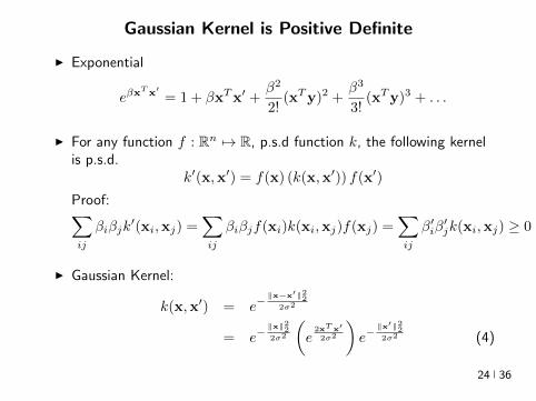
Gaussian Kernel is Positive Definite
I Exponential
eβxTxprime = 1 + βxTxprime +
β2
2(xTy)2 +
β3
3(xTy)3 +
I For any function f Rn 7rarr R psd function k the following kernelis psd
kprime(xxprime) = f(x) (k(xxprime)) f(xprime)
Proofsumij
βiβjkprime(xixj) =
sumij
βiβjf(xi)k(xixj)f(xj) =sumij
βprimeiβprimejk(xixj) ge 0
I Gaussian Kernel
k(xxprime) = eminusxminusxprime22
2σ2
= eminusx222σ2
(e
2xT xprime2σ2
)eminusxprime222σ2 (4)
24 36
The Mathematical Naturalness of Kernel Methods
I Data X isin Rd Models isin H X 7rarr R
I Geometry in H inner product 〈middot middot〉H norm middot H (Hilbert Spaces)I Theorem All nice Hilbert spaces are generated by a symmetric
positive definite function (the kernel) k(xxprime) on X times XI if f g isin H close ie f minus gH small then f(x) g(x) close forallx isin X I Reproducing Kernel Hilbert Spaces (RKHSs) Hilbert space H
that admit a reproducing kernel ie a function k(xxprime) satisfying
(i) forallx isin X k(middotx) isin H(ii) 〈f k(middotx)〉H = f(x)
I Reproducing kernels are symmetric psdsumij
βiβjk(xixj) = 〈sumi
βik(middotxi)sumi
βik(middotxi)〉H
= sumi
βik(middotxi)2H ge 0 (5)
I (Moore-Aronsjan 1950) Symmetric psd functions arereproducing kernels for some (unique) RKHS Hk
25 36
The Mathematical Naturalness of Kernel Methods
I Data X isin Rd Models isin H X 7rarr RI Geometry in H inner product 〈middot middot〉H norm middot H (Hilbert Spaces)
I Theorem All nice Hilbert spaces are generated by a symmetricpositive definite function (the kernel) k(xxprime) on X times X
I if f g isin H close ie f minus gH small then f(x) g(x) close forallx isin X I Reproducing Kernel Hilbert Spaces (RKHSs) Hilbert space H
that admit a reproducing kernel ie a function k(xxprime) satisfying
(i) forallx isin X k(middotx) isin H(ii) 〈f k(middotx)〉H = f(x)
I Reproducing kernels are symmetric psdsumij
βiβjk(xixj) = 〈sumi
βik(middotxi)sumi
βik(middotxi)〉H
= sumi
βik(middotxi)2H ge 0 (5)
I (Moore-Aronsjan 1950) Symmetric psd functions arereproducing kernels for some (unique) RKHS Hk
25 36
The Mathematical Naturalness of Kernel Methods
I Data X isin Rd Models isin H X 7rarr RI Geometry in H inner product 〈middot middot〉H norm middot H (Hilbert Spaces)I Theorem All nice Hilbert spaces are generated by a symmetric
positive definite function (the kernel) k(xxprime) on X times XI if f g isin H close ie f minus gH small then f(x) g(x) close forallx isin X
I Reproducing Kernel Hilbert Spaces (RKHSs) Hilbert space Hthat admit a reproducing kernel ie a function k(xxprime) satisfying
(i) forallx isin X k(middotx) isin H(ii) 〈f k(middotx)〉H = f(x)
I Reproducing kernels are symmetric psdsumij
βiβjk(xixj) = 〈sumi
βik(middotxi)sumi
βik(middotxi)〉H
= sumi
βik(middotxi)2H ge 0 (5)
I (Moore-Aronsjan 1950) Symmetric psd functions arereproducing kernels for some (unique) RKHS Hk
25 36
The Mathematical Naturalness of Kernel Methods
I Data X isin Rd Models isin H X 7rarr RI Geometry in H inner product 〈middot middot〉H norm middot H (Hilbert Spaces)I Theorem All nice Hilbert spaces are generated by a symmetric
positive definite function (the kernel) k(xxprime) on X times XI if f g isin H close ie f minus gH small then f(x) g(x) close forallx isin X I Reproducing Kernel Hilbert Spaces (RKHSs) Hilbert space H
that admit a reproducing kernel ie a function k(xxprime) satisfying
(i) forallx isin X k(middotx) isin H(ii) 〈f k(middotx)〉H = f(x)
I Reproducing kernels are symmetric psdsumij
βiβjk(xixj) = 〈sumi
βik(middotxi)sumi
βik(middotxi)〉H
= sumi
βik(middotxi)2H ge 0 (5)
I (Moore-Aronsjan 1950) Symmetric psd functions arereproducing kernels for some (unique) RKHS Hk
25 36
The Mathematical Naturalness of Kernel Methods
I Data X isin Rd Models isin H X 7rarr RI Geometry in H inner product 〈middot middot〉H norm middot H (Hilbert Spaces)I Theorem All nice Hilbert spaces are generated by a symmetric
positive definite function (the kernel) k(xxprime) on X times XI if f g isin H close ie f minus gH small then f(x) g(x) close forallx isin X I Reproducing Kernel Hilbert Spaces (RKHSs) Hilbert space H
that admit a reproducing kernel ie a function k(xxprime) satisfying
(i) forallx isin X k(middotx) isin H(ii) 〈f k(middotx)〉H = f(x)
I Reproducing kernels are symmetric psdsumij
βiβjk(xixj) = 〈sumi
βik(middotxi)sumi
βik(middotxi)〉H
= sumi
βik(middotxi)2H ge 0 (5)
I (Moore-Aronsjan 1950) Symmetric psd functions arereproducing kernels for some (unique) RKHS Hk 25 36
Kernel Methods Summary
I Symm pos def function k(x z) on input domain X sub Rd
I k hArr rich Reproducing Kernel Hilbert Space (RKHS) Hk ofreal-valued functions with inner product 〈middot middot〉k and norm middot k
I Regularized Risk Minimization hArr Linear models in an implicithigh-dimensional (often infinite-dimensional) feature space
f = arg minfisinHk
1
n
nsumi=1
V (yi f(xi)) + λf2Hk xi isin Rd
I Representer Theorem f(x) =sumni=1 αik(xxi)
26 36
Shallow and Deep Function Spaces
I What does it mean to understand a function space
ndash Linear f(x) = wTxw isin Rd
ndash Polynomial f(x) = wT Ψ(x)w isin Rs
ndash RKHS balls f isin Hk fk lt γ [like vM le 1]
I Shallow nets f(x) = wTσ(Wx) (w isin RdW isin Rs)ndash For srarrinfin W sim p σ(u) = eminusiu approximates Gaussian kernel
methodsndash Theorem [Bochner 1937] One-to-one correspondence between k
and a density p such that
k(x z) = ψ(xminus z) =
intRdeminusi(xminusz)Twp(w)dw asymp 1
s
ssumj=1
eminusi(xminusz)Twj
Gaussian kernel k(x z) = eminusxminusz22
2σ2 lArrrArr p = N (0 σminus2Id)ndash Similar integral approx relates ReLU to the arc-cosine kernelndash Optimization versus Randomization
27 36
Shallow and Deep Function Spaces
I What does it mean to understand a function space
ndash Linear f(x) = wTxw isin Rd
ndash Polynomial f(x) = wT Ψ(x)w isin Rs
ndash RKHS balls f isin Hk fk lt γ [like vM le 1]
I Shallow nets f(x) = wTσ(Wx) (w isin RdW isin Rs)ndash For srarrinfin W sim p σ(u) = eminusiu approximates Gaussian kernel
methodsndash Theorem [Bochner 1937] One-to-one correspondence between k
and a density p such that
k(x z) = ψ(xminus z) =
intRdeminusi(xminusz)Twp(w)dw asymp 1
s
ssumj=1
eminusi(xminusz)Twj
Gaussian kernel k(x z) = eminusxminusz22
2σ2 lArrrArr p = N (0 σminus2Id)ndash Similar integral approx relates ReLU to the arc-cosine kernelndash Optimization versus Randomization
27 36
Shallow and Deep Function Spaces
I What does it mean to understand a function space
ndash Linear f(x) = wTxw isin Rd
ndash Polynomial f(x) = wT Ψ(x)w isin Rs
ndash RKHS balls f isin Hk fk lt γ [like vM le 1]
I Shallow nets f(x) = wTσ(Wx) (w isin RdW isin Rs)ndash For srarrinfin W sim p σ(u) = eminusiu approximates Gaussian kernel
methodsndash Theorem [Bochner 1937] One-to-one correspondence between k
and a density p such that
k(x z) = ψ(xminus z) =
intRdeminusi(xminusz)Twp(w)dw asymp 1
s
ssumj=1
eminusi(xminusz)Twj
Gaussian kernel k(x z) = eminusxminusz22
2σ2 lArrrArr p = N (0 σminus2Id)ndash Similar integral approx relates ReLU to the arc-cosine kernelndash Optimization versus Randomization
27 36
Shallow and Deep Function Spaces
I What does it mean to understand a function space
ndash Linear f(x) = wTxw isin Rd
ndash Polynomial f(x) = wT Ψ(x)w isin Rs
ndash RKHS balls f isin Hk fk lt γ [like vM le 1]
I Shallow nets f(x) = wTσ(Wx) (w isin RdW isin Rs)
ndash For srarrinfin W sim p σ(u) = eminusiu approximates Gaussian kernelmethods
ndash Theorem [Bochner 1937] One-to-one correspondence between kand a density p such that
k(x z) = ψ(xminus z) =
intRdeminusi(xminusz)Twp(w)dw asymp 1
s
ssumj=1
eminusi(xminusz)Twj
Gaussian kernel k(x z) = eminusxminusz22
2σ2 lArrrArr p = N (0 σminus2Id)ndash Similar integral approx relates ReLU to the arc-cosine kernelndash Optimization versus Randomization
27 36
Shallow and Deep Function Spaces
I What does it mean to understand a function space
ndash Linear f(x) = wTxw isin Rd
ndash Polynomial f(x) = wT Ψ(x)w isin Rs
ndash RKHS balls f isin Hk fk lt γ [like vM le 1]
I Shallow nets f(x) = wTσ(Wx) (w isin RdW isin Rs)ndash For srarrinfin W sim p σ(u) = eminusiu approximates Gaussian kernel
methodsndash Theorem [Bochner 1937] One-to-one correspondence between k
and a density p such that
k(x z) = ψ(xminus z) =
intRdeminusi(xminusz)Twp(w)dw asymp 1
s
ssumj=1
eminusi(xminusz)Twj
Gaussian kernel k(x z) = eminusxminusz22
2σ2 lArrrArr p = N (0 σminus2Id)ndash Similar integral approx relates ReLU to the arc-cosine kernelndash Optimization versus Randomization
27 36
Expressivity of Deep Nets Linear Regions
I The ReLU map f(x) = max(Wx 0)W isin Rwtimesn is piecewise linear
I A piece is a connected region (a convex polytope) of Rd with sharedsparsity pattern in activations
I (Zaslavsky 1975) Number of linear regions formed by an arrangement of
s hyperplanes in d-dimensions in general position issumd
i=0
(si
)I Composition of ReLU maps is also piecewise linear
I (Raghu et al 2017 Pascano et al 2014 Montufar 2014) Number oflinear regions grows as O(wnd) for a composition of d ReLU maps(nrarr brarr brarr b rarr b) each of width w
I (Safran and Shamir 2017)
ndash 1[x le 1] x isin Rd ε-accurate 3-layer network with O(dε) neurons but cannot be approximated with
accuracy higher than O(1d4) using 2-layer networks unless width is exponential in d
28 36
Expressivity of Deep Nets Linear Regions
I The ReLU map f(x) = max(Wx 0)W isin Rwtimesn is piecewise linear
I A piece is a connected region (a convex polytope) of Rd with sharedsparsity pattern in activations
I (Zaslavsky 1975) Number of linear regions formed by an arrangement of
s hyperplanes in d-dimensions in general position issumd
i=0
(si
)I Composition of ReLU maps is also piecewise linear
I (Raghu et al 2017 Pascano et al 2014 Montufar 2014) Number oflinear regions grows as O(wnd) for a composition of d ReLU maps(nrarr brarr brarr b rarr b) each of width w
I (Safran and Shamir 2017)
ndash 1[x le 1] x isin Rd ε-accurate 3-layer network with O(dε) neurons but cannot be approximated with
accuracy higher than O(1d4) using 2-layer networks unless width is exponential in d
28 36
Expressivity of Deep Nets Linear Regions
I The ReLU map f(x) = max(Wx 0)W isin Rwtimesn is piecewise linear
I A piece is a connected region (a convex polytope) of Rd with sharedsparsity pattern in activations
I (Zaslavsky 1975) Number of linear regions formed by an arrangement of
s hyperplanes in d-dimensions in general position issumd
i=0
(si
)
I Composition of ReLU maps is also piecewise linear
I (Raghu et al 2017 Pascano et al 2014 Montufar 2014) Number oflinear regions grows as O(wnd) for a composition of d ReLU maps(nrarr brarr brarr b rarr b) each of width w
I (Safran and Shamir 2017)
ndash 1[x le 1] x isin Rd ε-accurate 3-layer network with O(dε) neurons but cannot be approximated with
accuracy higher than O(1d4) using 2-layer networks unless width is exponential in d
28 36
Expressivity of Deep Nets Linear Regions
I The ReLU map f(x) = max(Wx 0)W isin Rwtimesn is piecewise linear
I A piece is a connected region (a convex polytope) of Rd with sharedsparsity pattern in activations
I (Zaslavsky 1975) Number of linear regions formed by an arrangement of
s hyperplanes in d-dimensions in general position issumd
i=0
(si
)I Composition of ReLU maps is also piecewise linear
I (Raghu et al 2017 Pascano et al 2014 Montufar 2014) Number oflinear regions grows as O(wnd) for a composition of d ReLU maps(nrarr brarr brarr b rarr b) each of width w
I (Safran and Shamir 2017)
ndash 1[x le 1] x isin Rd ε-accurate 3-layer network with O(dε) neurons but cannot be approximated with
accuracy higher than O(1d4) using 2-layer networks unless width is exponential in d28 36
Expressivity of Deep Nets Trajectory Length
I (Raghu et al 2017) Trajectory Length (ldquogeneralized operator normrdquo)How much is a curve in the input space stretched by a layer in thenetwork
29 36
Expressivity of Deep Nets Trajectory Length
I (Raghu et al 2017) Trajectory Length (ldquogeneralized operator normrdquo)How much is a curve in the input space stretched by a layer in thenetwork
29 36
Expressivity and Generalization
I Expressiveness equiv capacity to fit random noise =rArr susceptibility tooverfitting (VC dimension Rademacher Complexity)
I Zhang et al 2017 Famous CNNs easily fit random labels
ndash Over-parameterized (n=12M psim 60M) but structuredndash Domain-knowledge baked in does not constraint expressiveness
I CNNs tend to generalize even without regularization (explicit and implicit)
I For linear regression SGD returns minimum norm solution
30 36
Expressivity and Generalization
I Expressiveness equiv capacity to fit random noise =rArr susceptibility tooverfitting (VC dimension Rademacher Complexity)
I Zhang et al 2017 Famous CNNs easily fit random labels
ndash Over-parameterized (n=12M psim 60M) but structuredndash Domain-knowledge baked in does not constraint expressiveness
I CNNs tend to generalize even without regularization (explicit and implicit)
I For linear regression SGD returns minimum norm solution
30 36
Expressivity and Generalization
I Expressiveness equiv capacity to fit random noise =rArr susceptibility tooverfitting (VC dimension Rademacher Complexity)
I Zhang et al 2017 Famous CNNs easily fit random labels
ndash Over-parameterized (n=12M psim 60M) but structuredndash Domain-knowledge baked in does not constraint expressiveness
I CNNs tend to generalize even without regularization (explicit and implicit)
I For linear regression SGD returns minimum norm solution
30 36
Optimization Landscape Symmetry and Saddle Points
I Folklore lots of equivalent good local minI Classification of critical points based on Hessian spectrumI Permutation and Scaling symmetries
I Thm [Lee et al 2016 Anadkumar Ge] For the short-step gradientmethod the basin of attraction of strict saddle points (atleast onenegative eigenvalue) has measure zero
31 36
Optimization Landscape Symmetry and Saddle Points
I Folklore lots of equivalent good local minI Classification of critical points based on Hessian spectrumI Permutation and Scaling symmetries
I Thm [Lee et al 2016 Anadkumar Ge] For the short-step gradientmethod the basin of attraction of strict saddle points (atleast onenegative eigenvalue) has measure zero
31 36
Optimization Landscape Symmetry and Saddle Points
I Folklore lots of equivalent good local minI Classification of critical points based on Hessian spectrumI Permutation and Scaling symmetries
I Thm [Lee et al 2016 Anadkumar Ge] For the short-step gradientmethod the basin of attraction of strict saddle points (atleast onenegative eigenvalue) has measure zero
31 36
Optimization Landscape Sharp Minima and Stability
Keskar et al 2017 On large-batch training for DL Generalization Gap and Sharp Minima
32 36
Deep Learning Computational Graphs TensorFlow
tensorfloworg
I Tensors-in Tensors-out
I Evergrowing list of Tensor-Ops (PythonC++)
f(xw)
[partf
partx
]T v
[partf
partw
]T v
I Automatic Differentiation Reverse mode
partxL
partxi=sumirarrj
partxL
partxj
partxj
partxi
33 36
Computational Graphs and TensorFlow
tensorfloworg
I SGD with minibatches
wk+1 = wk minus ηlsumi=1
partli
partw
∣∣∣wt
I Model Parallelism Assign independent paths tothreads GPUs
I Data Parallelism create Graph replicas on differentmachines
I Mobile TensorFlow
34 36
Computational Graphs and TensorFlow
tensorfloworg
35 36
Computational Graphs and TensorFlow
tensorfloworg
35 36
Computational Graphs and TensorFlow
tensorfloworg
35 36
Challenges and Opportunities
I Lots of fascinating unsolved problems
I Can you win Imagenet with Convex optimization
I Tools from polynomial optimization (global optimization deep-RL)
I Supervised to Semi-supervised to Unsupervised Learning
I Compact efficient real-time models (eliminateover-parametrization) for new form factors
I Exciting emerging world of Robotics Wearable ComputersIntelligent home devices Personal digital assistants
Google Internship Program
36 36
- anm0
- fdrm0
- fdrm5
The Mathematical Naturalness of Kernel Methods
I Data X isin Rd Models isin H X 7rarr RI Geometry in H inner product 〈middot middot〉H norm middot H (Hilbert Spaces)
I Theorem All nice Hilbert spaces are generated by a symmetricpositive definite function (the kernel) k(xxprime) on X times X
I if f g isin H close ie f minus gH small then f(x) g(x) close forallx isin X I Reproducing Kernel Hilbert Spaces (RKHSs) Hilbert space H
that admit a reproducing kernel ie a function k(xxprime) satisfying
(i) forallx isin X k(middotx) isin H(ii) 〈f k(middotx)〉H = f(x)
I Reproducing kernels are symmetric psdsumij
βiβjk(xixj) = 〈sumi
βik(middotxi)sumi
βik(middotxi)〉H
= sumi
βik(middotxi)2H ge 0 (5)
I (Moore-Aronsjan 1950) Symmetric psd functions arereproducing kernels for some (unique) RKHS Hk
25 36
The Mathematical Naturalness of Kernel Methods
I Data X isin Rd Models isin H X 7rarr RI Geometry in H inner product 〈middot middot〉H norm middot H (Hilbert Spaces)I Theorem All nice Hilbert spaces are generated by a symmetric
positive definite function (the kernel) k(xxprime) on X times XI if f g isin H close ie f minus gH small then f(x) g(x) close forallx isin X
I Reproducing Kernel Hilbert Spaces (RKHSs) Hilbert space Hthat admit a reproducing kernel ie a function k(xxprime) satisfying
(i) forallx isin X k(middotx) isin H(ii) 〈f k(middotx)〉H = f(x)
I Reproducing kernels are symmetric psdsumij
βiβjk(xixj) = 〈sumi
βik(middotxi)sumi
βik(middotxi)〉H
= sumi
βik(middotxi)2H ge 0 (5)
I (Moore-Aronsjan 1950) Symmetric psd functions arereproducing kernels for some (unique) RKHS Hk
25 36
The Mathematical Naturalness of Kernel Methods
I Data X isin Rd Models isin H X 7rarr RI Geometry in H inner product 〈middot middot〉H norm middot H (Hilbert Spaces)I Theorem All nice Hilbert spaces are generated by a symmetric
positive definite function (the kernel) k(xxprime) on X times XI if f g isin H close ie f minus gH small then f(x) g(x) close forallx isin X I Reproducing Kernel Hilbert Spaces (RKHSs) Hilbert space H
that admit a reproducing kernel ie a function k(xxprime) satisfying
(i) forallx isin X k(middotx) isin H(ii) 〈f k(middotx)〉H = f(x)
I Reproducing kernels are symmetric psdsumij
βiβjk(xixj) = 〈sumi
βik(middotxi)sumi
βik(middotxi)〉H
= sumi
βik(middotxi)2H ge 0 (5)
I (Moore-Aronsjan 1950) Symmetric psd functions arereproducing kernels for some (unique) RKHS Hk
25 36
The Mathematical Naturalness of Kernel Methods
I Data X isin Rd Models isin H X 7rarr RI Geometry in H inner product 〈middot middot〉H norm middot H (Hilbert Spaces)I Theorem All nice Hilbert spaces are generated by a symmetric
positive definite function (the kernel) k(xxprime) on X times XI if f g isin H close ie f minus gH small then f(x) g(x) close forallx isin X I Reproducing Kernel Hilbert Spaces (RKHSs) Hilbert space H
that admit a reproducing kernel ie a function k(xxprime) satisfying
(i) forallx isin X k(middotx) isin H(ii) 〈f k(middotx)〉H = f(x)
I Reproducing kernels are symmetric psdsumij
βiβjk(xixj) = 〈sumi
βik(middotxi)sumi
βik(middotxi)〉H
= sumi
βik(middotxi)2H ge 0 (5)
I (Moore-Aronsjan 1950) Symmetric psd functions arereproducing kernels for some (unique) RKHS Hk 25 36
Kernel Methods Summary
I Symm pos def function k(x z) on input domain X sub Rd
I k hArr rich Reproducing Kernel Hilbert Space (RKHS) Hk ofreal-valued functions with inner product 〈middot middot〉k and norm middot k
I Regularized Risk Minimization hArr Linear models in an implicithigh-dimensional (often infinite-dimensional) feature space
f = arg minfisinHk
1
n
nsumi=1
V (yi f(xi)) + λf2Hk xi isin Rd
I Representer Theorem f(x) =sumni=1 αik(xxi)
26 36
Shallow and Deep Function Spaces
I What does it mean to understand a function space
ndash Linear f(x) = wTxw isin Rd
ndash Polynomial f(x) = wT Ψ(x)w isin Rs
ndash RKHS balls f isin Hk fk lt γ [like vM le 1]
I Shallow nets f(x) = wTσ(Wx) (w isin RdW isin Rs)ndash For srarrinfin W sim p σ(u) = eminusiu approximates Gaussian kernel
methodsndash Theorem [Bochner 1937] One-to-one correspondence between k
and a density p such that
k(x z) = ψ(xminus z) =
intRdeminusi(xminusz)Twp(w)dw asymp 1
s
ssumj=1
eminusi(xminusz)Twj
Gaussian kernel k(x z) = eminusxminusz22
2σ2 lArrrArr p = N (0 σminus2Id)ndash Similar integral approx relates ReLU to the arc-cosine kernelndash Optimization versus Randomization
27 36
Shallow and Deep Function Spaces
I What does it mean to understand a function space
ndash Linear f(x) = wTxw isin Rd
ndash Polynomial f(x) = wT Ψ(x)w isin Rs
ndash RKHS balls f isin Hk fk lt γ [like vM le 1]
I Shallow nets f(x) = wTσ(Wx) (w isin RdW isin Rs)ndash For srarrinfin W sim p σ(u) = eminusiu approximates Gaussian kernel
methodsndash Theorem [Bochner 1937] One-to-one correspondence between k
and a density p such that
k(x z) = ψ(xminus z) =
intRdeminusi(xminusz)Twp(w)dw asymp 1
s
ssumj=1
eminusi(xminusz)Twj
Gaussian kernel k(x z) = eminusxminusz22
2σ2 lArrrArr p = N (0 σminus2Id)ndash Similar integral approx relates ReLU to the arc-cosine kernelndash Optimization versus Randomization
27 36
Shallow and Deep Function Spaces
I What does it mean to understand a function space
ndash Linear f(x) = wTxw isin Rd
ndash Polynomial f(x) = wT Ψ(x)w isin Rs
ndash RKHS balls f isin Hk fk lt γ [like vM le 1]
I Shallow nets f(x) = wTσ(Wx) (w isin RdW isin Rs)ndash For srarrinfin W sim p σ(u) = eminusiu approximates Gaussian kernel
methodsndash Theorem [Bochner 1937] One-to-one correspondence between k
and a density p such that
k(x z) = ψ(xminus z) =
intRdeminusi(xminusz)Twp(w)dw asymp 1
s
ssumj=1
eminusi(xminusz)Twj
Gaussian kernel k(x z) = eminusxminusz22
2σ2 lArrrArr p = N (0 σminus2Id)ndash Similar integral approx relates ReLU to the arc-cosine kernelndash Optimization versus Randomization
27 36
Shallow and Deep Function Spaces
I What does it mean to understand a function space
ndash Linear f(x) = wTxw isin Rd
ndash Polynomial f(x) = wT Ψ(x)w isin Rs
ndash RKHS balls f isin Hk fk lt γ [like vM le 1]
I Shallow nets f(x) = wTσ(Wx) (w isin RdW isin Rs)
ndash For srarrinfin W sim p σ(u) = eminusiu approximates Gaussian kernelmethods
ndash Theorem [Bochner 1937] One-to-one correspondence between kand a density p such that
k(x z) = ψ(xminus z) =
intRdeminusi(xminusz)Twp(w)dw asymp 1
s
ssumj=1
eminusi(xminusz)Twj
Gaussian kernel k(x z) = eminusxminusz22
2σ2 lArrrArr p = N (0 σminus2Id)ndash Similar integral approx relates ReLU to the arc-cosine kernelndash Optimization versus Randomization
27 36
Shallow and Deep Function Spaces
I What does it mean to understand a function space
ndash Linear f(x) = wTxw isin Rd
ndash Polynomial f(x) = wT Ψ(x)w isin Rs
ndash RKHS balls f isin Hk fk lt γ [like vM le 1]
I Shallow nets f(x) = wTσ(Wx) (w isin RdW isin Rs)ndash For srarrinfin W sim p σ(u) = eminusiu approximates Gaussian kernel
methodsndash Theorem [Bochner 1937] One-to-one correspondence between k
and a density p such that
k(x z) = ψ(xminus z) =
intRdeminusi(xminusz)Twp(w)dw asymp 1
s
ssumj=1
eminusi(xminusz)Twj
Gaussian kernel k(x z) = eminusxminusz22
2σ2 lArrrArr p = N (0 σminus2Id)ndash Similar integral approx relates ReLU to the arc-cosine kernelndash Optimization versus Randomization
27 36
Expressivity of Deep Nets Linear Regions
I The ReLU map f(x) = max(Wx 0)W isin Rwtimesn is piecewise linear
I A piece is a connected region (a convex polytope) of Rd with sharedsparsity pattern in activations
I (Zaslavsky 1975) Number of linear regions formed by an arrangement of
s hyperplanes in d-dimensions in general position issumd
i=0
(si
)I Composition of ReLU maps is also piecewise linear
I (Raghu et al 2017 Pascano et al 2014 Montufar 2014) Number oflinear regions grows as O(wnd) for a composition of d ReLU maps(nrarr brarr brarr b rarr b) each of width w
I (Safran and Shamir 2017)
ndash 1[x le 1] x isin Rd ε-accurate 3-layer network with O(dε) neurons but cannot be approximated with
accuracy higher than O(1d4) using 2-layer networks unless width is exponential in d
28 36
Expressivity of Deep Nets Linear Regions
I The ReLU map f(x) = max(Wx 0)W isin Rwtimesn is piecewise linear
I A piece is a connected region (a convex polytope) of Rd with sharedsparsity pattern in activations
I (Zaslavsky 1975) Number of linear regions formed by an arrangement of
s hyperplanes in d-dimensions in general position issumd
i=0
(si
)I Composition of ReLU maps is also piecewise linear
I (Raghu et al 2017 Pascano et al 2014 Montufar 2014) Number oflinear regions grows as O(wnd) for a composition of d ReLU maps(nrarr brarr brarr b rarr b) each of width w
I (Safran and Shamir 2017)
ndash 1[x le 1] x isin Rd ε-accurate 3-layer network with O(dε) neurons but cannot be approximated with
accuracy higher than O(1d4) using 2-layer networks unless width is exponential in d
28 36
Expressivity of Deep Nets Linear Regions
I The ReLU map f(x) = max(Wx 0)W isin Rwtimesn is piecewise linear
I A piece is a connected region (a convex polytope) of Rd with sharedsparsity pattern in activations
I (Zaslavsky 1975) Number of linear regions formed by an arrangement of
s hyperplanes in d-dimensions in general position issumd
i=0
(si
)
I Composition of ReLU maps is also piecewise linear
I (Raghu et al 2017 Pascano et al 2014 Montufar 2014) Number oflinear regions grows as O(wnd) for a composition of d ReLU maps(nrarr brarr brarr b rarr b) each of width w
I (Safran and Shamir 2017)
ndash 1[x le 1] x isin Rd ε-accurate 3-layer network with O(dε) neurons but cannot be approximated with
accuracy higher than O(1d4) using 2-layer networks unless width is exponential in d
28 36
Expressivity of Deep Nets Linear Regions
I The ReLU map f(x) = max(Wx 0)W isin Rwtimesn is piecewise linear
I A piece is a connected region (a convex polytope) of Rd with sharedsparsity pattern in activations
I (Zaslavsky 1975) Number of linear regions formed by an arrangement of
s hyperplanes in d-dimensions in general position issumd
i=0
(si
)I Composition of ReLU maps is also piecewise linear
I (Raghu et al 2017 Pascano et al 2014 Montufar 2014) Number oflinear regions grows as O(wnd) for a composition of d ReLU maps(nrarr brarr brarr b rarr b) each of width w
I (Safran and Shamir 2017)
ndash 1[x le 1] x isin Rd ε-accurate 3-layer network with O(dε) neurons but cannot be approximated with
accuracy higher than O(1d4) using 2-layer networks unless width is exponential in d28 36
Expressivity of Deep Nets Trajectory Length
I (Raghu et al 2017) Trajectory Length (ldquogeneralized operator normrdquo)How much is a curve in the input space stretched by a layer in thenetwork
29 36
Expressivity of Deep Nets Trajectory Length
I (Raghu et al 2017) Trajectory Length (ldquogeneralized operator normrdquo)How much is a curve in the input space stretched by a layer in thenetwork
29 36
Expressivity and Generalization
I Expressiveness equiv capacity to fit random noise =rArr susceptibility tooverfitting (VC dimension Rademacher Complexity)
I Zhang et al 2017 Famous CNNs easily fit random labels
ndash Over-parameterized (n=12M psim 60M) but structuredndash Domain-knowledge baked in does not constraint expressiveness
I CNNs tend to generalize even without regularization (explicit and implicit)
I For linear regression SGD returns minimum norm solution
30 36
Expressivity and Generalization
I Expressiveness equiv capacity to fit random noise =rArr susceptibility tooverfitting (VC dimension Rademacher Complexity)
I Zhang et al 2017 Famous CNNs easily fit random labels
ndash Over-parameterized (n=12M psim 60M) but structuredndash Domain-knowledge baked in does not constraint expressiveness
I CNNs tend to generalize even without regularization (explicit and implicit)
I For linear regression SGD returns minimum norm solution
30 36
Expressivity and Generalization
I Expressiveness equiv capacity to fit random noise =rArr susceptibility tooverfitting (VC dimension Rademacher Complexity)
I Zhang et al 2017 Famous CNNs easily fit random labels
ndash Over-parameterized (n=12M psim 60M) but structuredndash Domain-knowledge baked in does not constraint expressiveness
I CNNs tend to generalize even without regularization (explicit and implicit)
I For linear regression SGD returns minimum norm solution
30 36
Optimization Landscape Symmetry and Saddle Points
I Folklore lots of equivalent good local minI Classification of critical points based on Hessian spectrumI Permutation and Scaling symmetries
I Thm [Lee et al 2016 Anadkumar Ge] For the short-step gradientmethod the basin of attraction of strict saddle points (atleast onenegative eigenvalue) has measure zero
31 36
Optimization Landscape Symmetry and Saddle Points
I Folklore lots of equivalent good local minI Classification of critical points based on Hessian spectrumI Permutation and Scaling symmetries
I Thm [Lee et al 2016 Anadkumar Ge] For the short-step gradientmethod the basin of attraction of strict saddle points (atleast onenegative eigenvalue) has measure zero
31 36
Optimization Landscape Symmetry and Saddle Points
I Folklore lots of equivalent good local minI Classification of critical points based on Hessian spectrumI Permutation and Scaling symmetries
I Thm [Lee et al 2016 Anadkumar Ge] For the short-step gradientmethod the basin of attraction of strict saddle points (atleast onenegative eigenvalue) has measure zero
31 36
Optimization Landscape Sharp Minima and Stability
Keskar et al 2017 On large-batch training for DL Generalization Gap and Sharp Minima
32 36
Deep Learning Computational Graphs TensorFlow
tensorfloworg
I Tensors-in Tensors-out
I Evergrowing list of Tensor-Ops (PythonC++)
f(xw)
[partf
partx
]T v
[partf
partw
]T v
I Automatic Differentiation Reverse mode
partxL
partxi=sumirarrj
partxL
partxj
partxj
partxi
33 36
Computational Graphs and TensorFlow
tensorfloworg
I SGD with minibatches
wk+1 = wk minus ηlsumi=1
partli
partw
∣∣∣wt
I Model Parallelism Assign independent paths tothreads GPUs
I Data Parallelism create Graph replicas on differentmachines
I Mobile TensorFlow
34 36
Computational Graphs and TensorFlow
tensorfloworg
35 36
Computational Graphs and TensorFlow
tensorfloworg
35 36
Computational Graphs and TensorFlow
tensorfloworg
35 36
Challenges and Opportunities
I Lots of fascinating unsolved problems
I Can you win Imagenet with Convex optimization
I Tools from polynomial optimization (global optimization deep-RL)
I Supervised to Semi-supervised to Unsupervised Learning
I Compact efficient real-time models (eliminateover-parametrization) for new form factors
I Exciting emerging world of Robotics Wearable ComputersIntelligent home devices Personal digital assistants
Google Internship Program
36 36
- anm0
- fdrm0
- fdrm5

The Mathematical Naturalness of Kernel Methods
I Data X isin Rd Models isin H X 7rarr RI Geometry in H inner product 〈middot middot〉H norm middot H (Hilbert Spaces)I Theorem All nice Hilbert spaces are generated by a symmetric
positive definite function (the kernel) k(xxprime) on X times XI if f g isin H close ie f minus gH small then f(x) g(x) close forallx isin X I Reproducing Kernel Hilbert Spaces (RKHSs) Hilbert space H
that admit a reproducing kernel ie a function k(xxprime) satisfying
(i) forallx isin X k(middotx) isin H(ii) 〈f k(middotx)〉H = f(x)
I Reproducing kernels are symmetric psdsumij
βiβjk(xixj) = 〈sumi
βik(middotxi)sumi
βik(middotxi)〉H
= sumi
βik(middotxi)2H ge 0 (5)
I (Moore-Aronsjan 1950) Symmetric psd functions arereproducing kernels for some (unique) RKHS Hk 25 36
Kernel Methods Summary
I Symm pos def function k(x z) on input domain X sub Rd
I k hArr rich Reproducing Kernel Hilbert Space (RKHS) Hk ofreal-valued functions with inner product 〈middot middot〉k and norm middot k
I Regularized Risk Minimization hArr Linear models in an implicithigh-dimensional (often infinite-dimensional) feature space
f = arg minfisinHk
1
n
nsumi=1
V (yi f(xi)) + λf2Hk xi isin Rd
I Representer Theorem f(x) =sumni=1 αik(xxi)
26 36
Shallow and Deep Function Spaces
I What does it mean to understand a function space
ndash Linear f(x) = wTxw isin Rd
ndash Polynomial f(x) = wT Ψ(x)w isin Rs
ndash RKHS balls f isin Hk fk lt γ [like vM le 1]
I Shallow nets f(x) = wTσ(Wx) (w isin RdW isin Rs)ndash For srarrinfin W sim p σ(u) = eminusiu approximates Gaussian kernel
methodsndash Theorem [Bochner 1937] One-to-one correspondence between k
and a density p such that
k(x z) = ψ(xminus z) =
intRdeminusi(xminusz)Twp(w)dw asymp 1
s
ssumj=1
eminusi(xminusz)Twj
Gaussian kernel k(x z) = eminusxminusz22
2σ2 lArrrArr p = N (0 σminus2Id)ndash Similar integral approx relates ReLU to the arc-cosine kernelndash Optimization versus Randomization
27 36
Shallow and Deep Function Spaces
I What does it mean to understand a function space
ndash Linear f(x) = wTxw isin Rd
ndash Polynomial f(x) = wT Ψ(x)w isin Rs
ndash RKHS balls f isin Hk fk lt γ [like vM le 1]
I Shallow nets f(x) = wTσ(Wx) (w isin RdW isin Rs)ndash For srarrinfin W sim p σ(u) = eminusiu approximates Gaussian kernel
methodsndash Theorem [Bochner 1937] One-to-one correspondence between k
and a density p such that
k(x z) = ψ(xminus z) =
intRdeminusi(xminusz)Twp(w)dw asymp 1
s
ssumj=1
eminusi(xminusz)Twj
Gaussian kernel k(x z) = eminusxminusz22
2σ2 lArrrArr p = N (0 σminus2Id)ndash Similar integral approx relates ReLU to the arc-cosine kernelndash Optimization versus Randomization
27 36
Shallow and Deep Function Spaces
I What does it mean to understand a function space
ndash Linear f(x) = wTxw isin Rd
ndash Polynomial f(x) = wT Ψ(x)w isin Rs
ndash RKHS balls f isin Hk fk lt γ [like vM le 1]
I Shallow nets f(x) = wTσ(Wx) (w isin RdW isin Rs)ndash For srarrinfin W sim p σ(u) = eminusiu approximates Gaussian kernel
methodsndash Theorem [Bochner 1937] One-to-one correspondence between k
and a density p such that
k(x z) = ψ(xminus z) =
intRdeminusi(xminusz)Twp(w)dw asymp 1
s
ssumj=1
eminusi(xminusz)Twj
Gaussian kernel k(x z) = eminusxminusz22
2σ2 lArrrArr p = N (0 σminus2Id)ndash Similar integral approx relates ReLU to the arc-cosine kernelndash Optimization versus Randomization
27 36
Shallow and Deep Function Spaces
I What does it mean to understand a function space
ndash Linear f(x) = wTxw isin Rd
ndash Polynomial f(x) = wT Ψ(x)w isin Rs
ndash RKHS balls f isin Hk fk lt γ [like vM le 1]
I Shallow nets f(x) = wTσ(Wx) (w isin RdW isin Rs)
ndash For srarrinfin W sim p σ(u) = eminusiu approximates Gaussian kernelmethods
ndash Theorem [Bochner 1937] One-to-one correspondence between kand a density p such that
k(x z) = ψ(xminus z) =
intRdeminusi(xminusz)Twp(w)dw asymp 1
s
ssumj=1
eminusi(xminusz)Twj
Gaussian kernel k(x z) = eminusxminusz22
2σ2 lArrrArr p = N (0 σminus2Id)ndash Similar integral approx relates ReLU to the arc-cosine kernelndash Optimization versus Randomization
27 36
Shallow and Deep Function Spaces
I What does it mean to understand a function space
ndash Linear f(x) = wTxw isin Rd
ndash Polynomial f(x) = wT Ψ(x)w isin Rs
ndash RKHS balls f isin Hk fk lt γ [like vM le 1]
I Shallow nets f(x) = wTσ(Wx) (w isin RdW isin Rs)ndash For srarrinfin W sim p σ(u) = eminusiu approximates Gaussian kernel
methodsndash Theorem [Bochner 1937] One-to-one correspondence between k
and a density p such that
k(x z) = ψ(xminus z) =
intRdeminusi(xminusz)Twp(w)dw asymp 1
s
ssumj=1
eminusi(xminusz)Twj
Gaussian kernel k(x z) = eminusxminusz22
2σ2 lArrrArr p = N (0 σminus2Id)ndash Similar integral approx relates ReLU to the arc-cosine kernelndash Optimization versus Randomization
27 36
Expressivity of Deep Nets Linear Regions
I The ReLU map f(x) = max(Wx 0)W isin Rwtimesn is piecewise linear
I A piece is a connected region (a convex polytope) of Rd with sharedsparsity pattern in activations
I (Zaslavsky 1975) Number of linear regions formed by an arrangement of
s hyperplanes in d-dimensions in general position issumd
i=0
(si
)I Composition of ReLU maps is also piecewise linear
I (Raghu et al 2017 Pascano et al 2014 Montufar 2014) Number oflinear regions grows as O(wnd) for a composition of d ReLU maps(nrarr brarr brarr b rarr b) each of width w
I (Safran and Shamir 2017)
ndash 1[x le 1] x isin Rd ε-accurate 3-layer network with O(dε) neurons but cannot be approximated with
accuracy higher than O(1d4) using 2-layer networks unless width is exponential in d
28 36
Expressivity of Deep Nets Linear Regions
I The ReLU map f(x) = max(Wx 0)W isin Rwtimesn is piecewise linear
I A piece is a connected region (a convex polytope) of Rd with sharedsparsity pattern in activations
I (Zaslavsky 1975) Number of linear regions formed by an arrangement of
s hyperplanes in d-dimensions in general position issumd
i=0
(si
)I Composition of ReLU maps is also piecewise linear
I (Raghu et al 2017 Pascano et al 2014 Montufar 2014) Number oflinear regions grows as O(wnd) for a composition of d ReLU maps(nrarr brarr brarr b rarr b) each of width w
I (Safran and Shamir 2017)
ndash 1[x le 1] x isin Rd ε-accurate 3-layer network with O(dε) neurons but cannot be approximated with
accuracy higher than O(1d4) using 2-layer networks unless width is exponential in d
28 36
Expressivity of Deep Nets Linear Regions
I The ReLU map f(x) = max(Wx 0)W isin Rwtimesn is piecewise linear
I A piece is a connected region (a convex polytope) of Rd with sharedsparsity pattern in activations
I (Zaslavsky 1975) Number of linear regions formed by an arrangement of
s hyperplanes in d-dimensions in general position issumd
i=0
(si
)
I Composition of ReLU maps is also piecewise linear
I (Raghu et al 2017 Pascano et al 2014 Montufar 2014) Number oflinear regions grows as O(wnd) for a composition of d ReLU maps(nrarr brarr brarr b rarr b) each of width w
I (Safran and Shamir 2017)
ndash 1[x le 1] x isin Rd ε-accurate 3-layer network with O(dε) neurons but cannot be approximated with
accuracy higher than O(1d4) using 2-layer networks unless width is exponential in d
28 36
Expressivity of Deep Nets Linear Regions
I The ReLU map f(x) = max(Wx 0)W isin Rwtimesn is piecewise linear
I A piece is a connected region (a convex polytope) of Rd with sharedsparsity pattern in activations
I (Zaslavsky 1975) Number of linear regions formed by an arrangement of
s hyperplanes in d-dimensions in general position issumd
i=0
(si
)I Composition of ReLU maps is also piecewise linear
I (Raghu et al 2017 Pascano et al 2014 Montufar 2014) Number oflinear regions grows as O(wnd) for a composition of d ReLU maps(nrarr brarr brarr b rarr b) each of width w
I (Safran and Shamir 2017)
ndash 1[x le 1] x isin Rd ε-accurate 3-layer network with O(dε) neurons but cannot be approximated with
accuracy higher than O(1d4) using 2-layer networks unless width is exponential in d28 36
Expressivity of Deep Nets Trajectory Length
I (Raghu et al 2017) Trajectory Length (ldquogeneralized operator normrdquo)How much is a curve in the input space stretched by a layer in thenetwork
29 36
Expressivity of Deep Nets Trajectory Length
I (Raghu et al 2017) Trajectory Length (ldquogeneralized operator normrdquo)How much is a curve in the input space stretched by a layer in thenetwork
29 36
Expressivity and Generalization
I Expressiveness equiv capacity to fit random noise =rArr susceptibility tooverfitting (VC dimension Rademacher Complexity)
I Zhang et al 2017 Famous CNNs easily fit random labels
ndash Over-parameterized (n=12M psim 60M) but structuredndash Domain-knowledge baked in does not constraint expressiveness
I CNNs tend to generalize even without regularization (explicit and implicit)
I For linear regression SGD returns minimum norm solution
30 36
Expressivity and Generalization
I Expressiveness equiv capacity to fit random noise =rArr susceptibility tooverfitting (VC dimension Rademacher Complexity)
I Zhang et al 2017 Famous CNNs easily fit random labels
ndash Over-parameterized (n=12M psim 60M) but structuredndash Domain-knowledge baked in does not constraint expressiveness
I CNNs tend to generalize even without regularization (explicit and implicit)
I For linear regression SGD returns minimum norm solution
30 36
Expressivity and Generalization
I Expressiveness equiv capacity to fit random noise =rArr susceptibility tooverfitting (VC dimension Rademacher Complexity)
I Zhang et al 2017 Famous CNNs easily fit random labels
ndash Over-parameterized (n=12M psim 60M) but structuredndash Domain-knowledge baked in does not constraint expressiveness
I CNNs tend to generalize even without regularization (explicit and implicit)
I For linear regression SGD returns minimum norm solution
30 36
Optimization Landscape Symmetry and Saddle Points
I Folklore lots of equivalent good local minI Classification of critical points based on Hessian spectrumI Permutation and Scaling symmetries
I Thm [Lee et al 2016 Anadkumar Ge] For the short-step gradientmethod the basin of attraction of strict saddle points (atleast onenegative eigenvalue) has measure zero
31 36
Optimization Landscape Symmetry and Saddle Points
I Folklore lots of equivalent good local minI Classification of critical points based on Hessian spectrumI Permutation and Scaling symmetries
I Thm [Lee et al 2016 Anadkumar Ge] For the short-step gradientmethod the basin of attraction of strict saddle points (atleast onenegative eigenvalue) has measure zero
31 36
Optimization Landscape Symmetry and Saddle Points
I Folklore lots of equivalent good local minI Classification of critical points based on Hessian spectrumI Permutation and Scaling symmetries
I Thm [Lee et al 2016 Anadkumar Ge] For the short-step gradientmethod the basin of attraction of strict saddle points (atleast onenegative eigenvalue) has measure zero
31 36
Optimization Landscape Sharp Minima and Stability
Keskar et al 2017 On large-batch training for DL Generalization Gap and Sharp Minima
32 36
Deep Learning Computational Graphs TensorFlow
tensorfloworg
I Tensors-in Tensors-out
I Evergrowing list of Tensor-Ops (PythonC++)
f(xw)
[partf
partx
]T v
[partf
partw
]T v
I Automatic Differentiation Reverse mode
partxL
partxi=sumirarrj
partxL
partxj
partxj
partxi
33 36
Computational Graphs and TensorFlow
tensorfloworg
I SGD with minibatches
wk+1 = wk minus ηlsumi=1
partli
partw
∣∣∣wt
I Model Parallelism Assign independent paths tothreads GPUs
I Data Parallelism create Graph replicas on differentmachines
I Mobile TensorFlow
34 36
Computational Graphs and TensorFlow
tensorfloworg
35 36
Computational Graphs and TensorFlow
tensorfloworg
35 36
Computational Graphs and TensorFlow
tensorfloworg
35 36
Challenges and Opportunities
I Lots of fascinating unsolved problems
I Can you win Imagenet with Convex optimization
I Tools from polynomial optimization (global optimization deep-RL)
I Supervised to Semi-supervised to Unsupervised Learning
I Compact efficient real-time models (eliminateover-parametrization) for new form factors
I Exciting emerging world of Robotics Wearable ComputersIntelligent home devices Personal digital assistants
Google Internship Program
36 36
- anm0
- fdrm0
- fdrm5
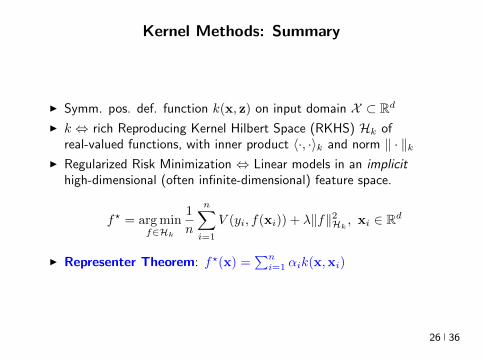

Shallow and Deep Function Spaces
I What does it mean to understand a function space
ndash Linear f(x) = wTxw isin Rd
ndash Polynomial f(x) = wT Ψ(x)w isin Rs
ndash RKHS balls f isin Hk fk lt γ [like vM le 1]
I Shallow nets f(x) = wTσ(Wx) (w isin RdW isin Rs)ndash For srarrinfin W sim p σ(u) = eminusiu approximates Gaussian kernel
methodsndash Theorem [Bochner 1937] One-to-one correspondence between k
and a density p such that
k(x z) = ψ(xminus z) =
intRdeminusi(xminusz)Twp(w)dw asymp 1
s
ssumj=1
eminusi(xminusz)Twj
Gaussian kernel k(x z) = eminusxminusz22
2σ2 lArrrArr p = N (0 σminus2Id)ndash Similar integral approx relates ReLU to the arc-cosine kernelndash Optimization versus Randomization
27 36
Shallow and Deep Function Spaces
I What does it mean to understand a function space
ndash Linear f(x) = wTxw isin Rd
ndash Polynomial f(x) = wT Ψ(x)w isin Rs
ndash RKHS balls f isin Hk fk lt γ [like vM le 1]
I Shallow nets f(x) = wTσ(Wx) (w isin RdW isin Rs)
ndash For srarrinfin W sim p σ(u) = eminusiu approximates Gaussian kernelmethods
ndash Theorem [Bochner 1937] One-to-one correspondence between kand a density p such that
k(x z) = ψ(xminus z) =
intRdeminusi(xminusz)Twp(w)dw asymp 1
s
ssumj=1
eminusi(xminusz)Twj
Gaussian kernel k(x z) = eminusxminusz22
2σ2 lArrrArr p = N (0 σminus2Id)ndash Similar integral approx relates ReLU to the arc-cosine kernelndash Optimization versus Randomization
27 36
Shallow and Deep Function Spaces
I What does it mean to understand a function space
ndash Linear f(x) = wTxw isin Rd
ndash Polynomial f(x) = wT Ψ(x)w isin Rs
ndash RKHS balls f isin Hk fk lt γ [like vM le 1]
I Shallow nets f(x) = wTσ(Wx) (w isin RdW isin Rs)ndash For srarrinfin W sim p σ(u) = eminusiu approximates Gaussian kernel
methodsndash Theorem [Bochner 1937] One-to-one correspondence between k
and a density p such that
k(x z) = ψ(xminus z) =
intRdeminusi(xminusz)Twp(w)dw asymp 1
s
ssumj=1
eminusi(xminusz)Twj
Gaussian kernel k(x z) = eminusxminusz22
2σ2 lArrrArr p = N (0 σminus2Id)ndash Similar integral approx relates ReLU to the arc-cosine kernelndash Optimization versus Randomization
27 36
Expressivity of Deep Nets Linear Regions
I The ReLU map f(x) = max(Wx 0)W isin Rwtimesn is piecewise linear
I A piece is a connected region (a convex polytope) of Rd with sharedsparsity pattern in activations
I (Zaslavsky 1975) Number of linear regions formed by an arrangement of
s hyperplanes in d-dimensions in general position issumd
i=0
(si
)I Composition of ReLU maps is also piecewise linear
I (Raghu et al 2017 Pascano et al 2014 Montufar 2014) Number oflinear regions grows as O(wnd) for a composition of d ReLU maps(nrarr brarr brarr b rarr b) each of width w
I (Safran and Shamir 2017)
ndash 1[x le 1] x isin Rd ε-accurate 3-layer network with O(dε) neurons but cannot be approximated with
accuracy higher than O(1d4) using 2-layer networks unless width is exponential in d
28 36
Expressivity of Deep Nets Linear Regions
I The ReLU map f(x) = max(Wx 0)W isin Rwtimesn is piecewise linear
I A piece is a connected region (a convex polytope) of Rd with sharedsparsity pattern in activations
I (Zaslavsky 1975) Number of linear regions formed by an arrangement of
s hyperplanes in d-dimensions in general position issumd
i=0
(si
)I Composition of ReLU maps is also piecewise linear
I (Raghu et al 2017 Pascano et al 2014 Montufar 2014) Number oflinear regions grows as O(wnd) for a composition of d ReLU maps(nrarr brarr brarr b rarr b) each of width w
I (Safran and Shamir 2017)
ndash 1[x le 1] x isin Rd ε-accurate 3-layer network with O(dε) neurons but cannot be approximated with
accuracy higher than O(1d4) using 2-layer networks unless width is exponential in d
28 36
Expressivity of Deep Nets Linear Regions
I The ReLU map f(x) = max(Wx 0)W isin Rwtimesn is piecewise linear
I A piece is a connected region (a convex polytope) of Rd with sharedsparsity pattern in activations
I (Zaslavsky 1975) Number of linear regions formed by an arrangement of
s hyperplanes in d-dimensions in general position issumd
i=0
(si
)
I Composition of ReLU maps is also piecewise linear
I (Raghu et al 2017 Pascano et al 2014 Montufar 2014) Number oflinear regions grows as O(wnd) for a composition of d ReLU maps(nrarr brarr brarr b rarr b) each of width w
I (Safran and Shamir 2017)
ndash 1[x le 1] x isin Rd ε-accurate 3-layer network with O(dε) neurons but cannot be approximated with
accuracy higher than O(1d4) using 2-layer networks unless width is exponential in d
28 36
Expressivity of Deep Nets Linear Regions
I The ReLU map f(x) = max(Wx 0)W isin Rwtimesn is piecewise linear
I A piece is a connected region (a convex polytope) of Rd with sharedsparsity pattern in activations
I (Zaslavsky 1975) Number of linear regions formed by an arrangement of
s hyperplanes in d-dimensions in general position issumd
i=0
(si
)I Composition of ReLU maps is also piecewise linear
I (Raghu et al 2017 Pascano et al 2014 Montufar 2014) Number oflinear regions grows as O(wnd) for a composition of d ReLU maps(nrarr brarr brarr b rarr b) each of width w
I (Safran and Shamir 2017)
ndash 1[x le 1] x isin Rd ε-accurate 3-layer network with O(dε) neurons but cannot be approximated with
accuracy higher than O(1d4) using 2-layer networks unless width is exponential in d28 36
Expressivity of Deep Nets Trajectory Length
I (Raghu et al 2017) Trajectory Length (ldquogeneralized operator normrdquo)How much is a curve in the input space stretched by a layer in thenetwork
29 36
Expressivity of Deep Nets Trajectory Length
I (Raghu et al 2017) Trajectory Length (ldquogeneralized operator normrdquo)How much is a curve in the input space stretched by a layer in thenetwork
29 36
Expressivity and Generalization
I Expressiveness equiv capacity to fit random noise =rArr susceptibility tooverfitting (VC dimension Rademacher Complexity)
I Zhang et al 2017 Famous CNNs easily fit random labels
ndash Over-parameterized (n=12M psim 60M) but structuredndash Domain-knowledge baked in does not constraint expressiveness
I CNNs tend to generalize even without regularization (explicit and implicit)
I For linear regression SGD returns minimum norm solution
30 36
Expressivity and Generalization
I Expressiveness equiv capacity to fit random noise =rArr susceptibility tooverfitting (VC dimension Rademacher Complexity)
I Zhang et al 2017 Famous CNNs easily fit random labels
ndash Over-parameterized (n=12M psim 60M) but structuredndash Domain-knowledge baked in does not constraint expressiveness
I CNNs tend to generalize even without regularization (explicit and implicit)
I For linear regression SGD returns minimum norm solution
30 36
Expressivity and Generalization
I Expressiveness equiv capacity to fit random noise =rArr susceptibility tooverfitting (VC dimension Rademacher Complexity)
I Zhang et al 2017 Famous CNNs easily fit random labels
ndash Over-parameterized (n=12M psim 60M) but structuredndash Domain-knowledge baked in does not constraint expressiveness
I CNNs tend to generalize even without regularization (explicit and implicit)
I For linear regression SGD returns minimum norm solution
30 36
Optimization Landscape Symmetry and Saddle Points
I Folklore lots of equivalent good local minI Classification of critical points based on Hessian spectrumI Permutation and Scaling symmetries
I Thm [Lee et al 2016 Anadkumar Ge] For the short-step gradientmethod the basin of attraction of strict saddle points (atleast onenegative eigenvalue) has measure zero
31 36
Optimization Landscape Symmetry and Saddle Points
I Folklore lots of equivalent good local minI Classification of critical points based on Hessian spectrumI Permutation and Scaling symmetries
I Thm [Lee et al 2016 Anadkumar Ge] For the short-step gradientmethod the basin of attraction of strict saddle points (atleast onenegative eigenvalue) has measure zero
31 36
Optimization Landscape Symmetry and Saddle Points
I Folklore lots of equivalent good local minI Classification of critical points based on Hessian spectrumI Permutation and Scaling symmetries
I Thm [Lee et al 2016 Anadkumar Ge] For the short-step gradientmethod the basin of attraction of strict saddle points (atleast onenegative eigenvalue) has measure zero
31 36
Optimization Landscape Sharp Minima and Stability
Keskar et al 2017 On large-batch training for DL Generalization Gap and Sharp Minima
32 36
Deep Learning Computational Graphs TensorFlow
tensorfloworg
I Tensors-in Tensors-out
I Evergrowing list of Tensor-Ops (PythonC++)
f(xw)
[partf
partx
]T v
[partf
partw
]T v
I Automatic Differentiation Reverse mode
partxL
partxi=sumirarrj
partxL
partxj
partxj
partxi
33 36
Computational Graphs and TensorFlow
tensorfloworg
I SGD with minibatches
wk+1 = wk minus ηlsumi=1
partli
partw
∣∣∣wt
I Model Parallelism Assign independent paths tothreads GPUs
I Data Parallelism create Graph replicas on differentmachines
I Mobile TensorFlow
34 36
Computational Graphs and TensorFlow
tensorfloworg
35 36
Computational Graphs and TensorFlow
tensorfloworg
35 36
Computational Graphs and TensorFlow
tensorfloworg
35 36
Challenges and Opportunities
I Lots of fascinating unsolved problems
I Can you win Imagenet with Convex optimization
I Tools from polynomial optimization (global optimization deep-RL)
I Supervised to Semi-supervised to Unsupervised Learning
I Compact efficient real-time models (eliminateover-parametrization) for new form factors
I Exciting emerging world of Robotics Wearable ComputersIntelligent home devices Personal digital assistants
Google Internship Program
36 36
- anm0
- fdrm0
- fdrm5
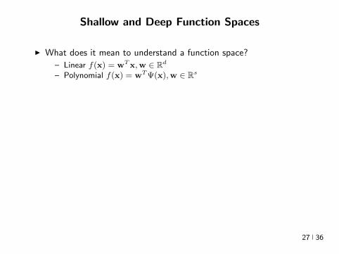
Shallow and Deep Function Spaces
I What does it mean to understand a function space
ndash Linear f(x) = wTxw isin Rd
ndash Polynomial f(x) = wT Ψ(x)w isin Rs
ndash RKHS balls f isin Hk fk lt γ [like vM le 1]
I Shallow nets f(x) = wTσ(Wx) (w isin RdW isin Rs)ndash For srarrinfin W sim p σ(u) = eminusiu approximates Gaussian kernel
methodsndash Theorem [Bochner 1937] One-to-one correspondence between k
and a density p such that
k(x z) = ψ(xminus z) =
intRdeminusi(xminusz)Twp(w)dw asymp 1
s
ssumj=1
eminusi(xminusz)Twj
Gaussian kernel k(x z) = eminusxminusz22
2σ2 lArrrArr p = N (0 σminus2Id)ndash Similar integral approx relates ReLU to the arc-cosine kernelndash Optimization versus Randomization
27 36
Shallow and Deep Function Spaces
I What does it mean to understand a function space
ndash Linear f(x) = wTxw isin Rd
ndash Polynomial f(x) = wT Ψ(x)w isin Rs
ndash RKHS balls f isin Hk fk lt γ [like vM le 1]
I Shallow nets f(x) = wTσ(Wx) (w isin RdW isin Rs)ndash For srarrinfin W sim p σ(u) = eminusiu approximates Gaussian kernel
methodsndash Theorem [Bochner 1937] One-to-one correspondence between k
and a density p such that
k(x z) = ψ(xminus z) =
intRdeminusi(xminusz)Twp(w)dw asymp 1
s
ssumj=1
eminusi(xminusz)Twj
Gaussian kernel k(x z) = eminusxminusz22
2σ2 lArrrArr p = N (0 σminus2Id)ndash Similar integral approx relates ReLU to the arc-cosine kernelndash Optimization versus Randomization
27 36
Shallow and Deep Function Spaces
I What does it mean to understand a function space
ndash Linear f(x) = wTxw isin Rd
ndash Polynomial f(x) = wT Ψ(x)w isin Rs
ndash RKHS balls f isin Hk fk lt γ [like vM le 1]
I Shallow nets f(x) = wTσ(Wx) (w isin RdW isin Rs)
ndash For srarrinfin W sim p σ(u) = eminusiu approximates Gaussian kernelmethods
ndash Theorem [Bochner 1937] One-to-one correspondence between kand a density p such that
k(x z) = ψ(xminus z) =
intRdeminusi(xminusz)Twp(w)dw asymp 1
s
ssumj=1
eminusi(xminusz)Twj
Gaussian kernel k(x z) = eminusxminusz22
2σ2 lArrrArr p = N (0 σminus2Id)ndash Similar integral approx relates ReLU to the arc-cosine kernelndash Optimization versus Randomization
27 36
Shallow and Deep Function Spaces
I What does it mean to understand a function space
ndash Linear f(x) = wTxw isin Rd
ndash Polynomial f(x) = wT Ψ(x)w isin Rs
ndash RKHS balls f isin Hk fk lt γ [like vM le 1]
I Shallow nets f(x) = wTσ(Wx) (w isin RdW isin Rs)ndash For srarrinfin W sim p σ(u) = eminusiu approximates Gaussian kernel
methodsndash Theorem [Bochner 1937] One-to-one correspondence between k
and a density p such that
k(x z) = ψ(xminus z) =
intRdeminusi(xminusz)Twp(w)dw asymp 1
s
ssumj=1
eminusi(xminusz)Twj
Gaussian kernel k(x z) = eminusxminusz22
2σ2 lArrrArr p = N (0 σminus2Id)ndash Similar integral approx relates ReLU to the arc-cosine kernelndash Optimization versus Randomization
27 36
Expressivity of Deep Nets Linear Regions
I The ReLU map f(x) = max(Wx 0)W isin Rwtimesn is piecewise linear
I A piece is a connected region (a convex polytope) of Rd with sharedsparsity pattern in activations
I (Zaslavsky 1975) Number of linear regions formed by an arrangement of
s hyperplanes in d-dimensions in general position issumd
i=0
(si
)I Composition of ReLU maps is also piecewise linear
I (Raghu et al 2017 Pascano et al 2014 Montufar 2014) Number oflinear regions grows as O(wnd) for a composition of d ReLU maps(nrarr brarr brarr b rarr b) each of width w
I (Safran and Shamir 2017)
ndash 1[x le 1] x isin Rd ε-accurate 3-layer network with O(dε) neurons but cannot be approximated with
accuracy higher than O(1d4) using 2-layer networks unless width is exponential in d
28 36
Expressivity of Deep Nets Linear Regions
I The ReLU map f(x) = max(Wx 0)W isin Rwtimesn is piecewise linear
I A piece is a connected region (a convex polytope) of Rd with sharedsparsity pattern in activations
I (Zaslavsky 1975) Number of linear regions formed by an arrangement of
s hyperplanes in d-dimensions in general position issumd
i=0
(si
)I Composition of ReLU maps is also piecewise linear
I (Raghu et al 2017 Pascano et al 2014 Montufar 2014) Number oflinear regions grows as O(wnd) for a composition of d ReLU maps(nrarr brarr brarr b rarr b) each of width w
I (Safran and Shamir 2017)
ndash 1[x le 1] x isin Rd ε-accurate 3-layer network with O(dε) neurons but cannot be approximated with
accuracy higher than O(1d4) using 2-layer networks unless width is exponential in d
28 36
Expressivity of Deep Nets Linear Regions
I The ReLU map f(x) = max(Wx 0)W isin Rwtimesn is piecewise linear
I A piece is a connected region (a convex polytope) of Rd with sharedsparsity pattern in activations
I (Zaslavsky 1975) Number of linear regions formed by an arrangement of
s hyperplanes in d-dimensions in general position issumd
i=0
(si
)
I Composition of ReLU maps is also piecewise linear
I (Raghu et al 2017 Pascano et al 2014 Montufar 2014) Number oflinear regions grows as O(wnd) for a composition of d ReLU maps(nrarr brarr brarr b rarr b) each of width w
I (Safran and Shamir 2017)
ndash 1[x le 1] x isin Rd ε-accurate 3-layer network with O(dε) neurons but cannot be approximated with
accuracy higher than O(1d4) using 2-layer networks unless width is exponential in d
28 36
Expressivity of Deep Nets Linear Regions
I The ReLU map f(x) = max(Wx 0)W isin Rwtimesn is piecewise linear
I A piece is a connected region (a convex polytope) of Rd with sharedsparsity pattern in activations
I (Zaslavsky 1975) Number of linear regions formed by an arrangement of
s hyperplanes in d-dimensions in general position issumd
i=0
(si
)I Composition of ReLU maps is also piecewise linear
I (Raghu et al 2017 Pascano et al 2014 Montufar 2014) Number oflinear regions grows as O(wnd) for a composition of d ReLU maps(nrarr brarr brarr b rarr b) each of width w
I (Safran and Shamir 2017)
ndash 1[x le 1] x isin Rd ε-accurate 3-layer network with O(dε) neurons but cannot be approximated with
accuracy higher than O(1d4) using 2-layer networks unless width is exponential in d28 36
Expressivity of Deep Nets Trajectory Length
I (Raghu et al 2017) Trajectory Length (ldquogeneralized operator normrdquo)How much is a curve in the input space stretched by a layer in thenetwork
29 36
Expressivity of Deep Nets Trajectory Length
I (Raghu et al 2017) Trajectory Length (ldquogeneralized operator normrdquo)How much is a curve in the input space stretched by a layer in thenetwork
29 36
Expressivity and Generalization
I Expressiveness equiv capacity to fit random noise =rArr susceptibility tooverfitting (VC dimension Rademacher Complexity)
I Zhang et al 2017 Famous CNNs easily fit random labels
ndash Over-parameterized (n=12M psim 60M) but structuredndash Domain-knowledge baked in does not constraint expressiveness
I CNNs tend to generalize even without regularization (explicit and implicit)
I For linear regression SGD returns minimum norm solution
30 36
Expressivity and Generalization
I Expressiveness equiv capacity to fit random noise =rArr susceptibility tooverfitting (VC dimension Rademacher Complexity)
I Zhang et al 2017 Famous CNNs easily fit random labels
ndash Over-parameterized (n=12M psim 60M) but structuredndash Domain-knowledge baked in does not constraint expressiveness
I CNNs tend to generalize even without regularization (explicit and implicit)
I For linear regression SGD returns minimum norm solution
30 36
Expressivity and Generalization
I Expressiveness equiv capacity to fit random noise =rArr susceptibility tooverfitting (VC dimension Rademacher Complexity)
I Zhang et al 2017 Famous CNNs easily fit random labels
ndash Over-parameterized (n=12M psim 60M) but structuredndash Domain-knowledge baked in does not constraint expressiveness
I CNNs tend to generalize even without regularization (explicit and implicit)
I For linear regression SGD returns minimum norm solution
30 36
Optimization Landscape Symmetry and Saddle Points
I Folklore lots of equivalent good local minI Classification of critical points based on Hessian spectrumI Permutation and Scaling symmetries
I Thm [Lee et al 2016 Anadkumar Ge] For the short-step gradientmethod the basin of attraction of strict saddle points (atleast onenegative eigenvalue) has measure zero
31 36
Optimization Landscape Symmetry and Saddle Points
I Folklore lots of equivalent good local minI Classification of critical points based on Hessian spectrumI Permutation and Scaling symmetries
I Thm [Lee et al 2016 Anadkumar Ge] For the short-step gradientmethod the basin of attraction of strict saddle points (atleast onenegative eigenvalue) has measure zero
31 36
Optimization Landscape Symmetry and Saddle Points
I Folklore lots of equivalent good local minI Classification of critical points based on Hessian spectrumI Permutation and Scaling symmetries
I Thm [Lee et al 2016 Anadkumar Ge] For the short-step gradientmethod the basin of attraction of strict saddle points (atleast onenegative eigenvalue) has measure zero
31 36
Optimization Landscape Sharp Minima and Stability
Keskar et al 2017 On large-batch training for DL Generalization Gap and Sharp Minima
32 36
Deep Learning Computational Graphs TensorFlow
tensorfloworg
I Tensors-in Tensors-out
I Evergrowing list of Tensor-Ops (PythonC++)
f(xw)
[partf
partx
]T v
[partf
partw
]T v
I Automatic Differentiation Reverse mode
partxL
partxi=sumirarrj
partxL
partxj
partxj
partxi
33 36
Computational Graphs and TensorFlow
tensorfloworg
I SGD with minibatches
wk+1 = wk minus ηlsumi=1
partli
partw
∣∣∣wt
I Model Parallelism Assign independent paths tothreads GPUs
I Data Parallelism create Graph replicas on differentmachines
I Mobile TensorFlow
34 36
Computational Graphs and TensorFlow
tensorfloworg
35 36
Computational Graphs and TensorFlow
tensorfloworg
35 36
Computational Graphs and TensorFlow
tensorfloworg
35 36
Challenges and Opportunities
I Lots of fascinating unsolved problems
I Can you win Imagenet with Convex optimization
I Tools from polynomial optimization (global optimization deep-RL)
I Supervised to Semi-supervised to Unsupervised Learning
I Compact efficient real-time models (eliminateover-parametrization) for new form factors
I Exciting emerging world of Robotics Wearable ComputersIntelligent home devices Personal digital assistants
Google Internship Program
36 36
- anm0
- fdrm0
- fdrm5

Shallow and Deep Function Spaces
I What does it mean to understand a function space
ndash Linear f(x) = wTxw isin Rd
ndash Polynomial f(x) = wT Ψ(x)w isin Rs
ndash RKHS balls f isin Hk fk lt γ [like vM le 1]
I Shallow nets f(x) = wTσ(Wx) (w isin RdW isin Rs)ndash For srarrinfin W sim p σ(u) = eminusiu approximates Gaussian kernel
methodsndash Theorem [Bochner 1937] One-to-one correspondence between k
and a density p such that
k(x z) = ψ(xminus z) =
intRdeminusi(xminusz)Twp(w)dw asymp 1
s
ssumj=1
eminusi(xminusz)Twj
Gaussian kernel k(x z) = eminusxminusz22
2σ2 lArrrArr p = N (0 σminus2Id)ndash Similar integral approx relates ReLU to the arc-cosine kernelndash Optimization versus Randomization
27 36
Shallow and Deep Function Spaces
I What does it mean to understand a function space
ndash Linear f(x) = wTxw isin Rd
ndash Polynomial f(x) = wT Ψ(x)w isin Rs
ndash RKHS balls f isin Hk fk lt γ [like vM le 1]
I Shallow nets f(x) = wTσ(Wx) (w isin RdW isin Rs)
ndash For srarrinfin W sim p σ(u) = eminusiu approximates Gaussian kernelmethods
ndash Theorem [Bochner 1937] One-to-one correspondence between kand a density p such that
k(x z) = ψ(xminus z) =
intRdeminusi(xminusz)Twp(w)dw asymp 1
s
ssumj=1
eminusi(xminusz)Twj
Gaussian kernel k(x z) = eminusxminusz22
2σ2 lArrrArr p = N (0 σminus2Id)ndash Similar integral approx relates ReLU to the arc-cosine kernelndash Optimization versus Randomization
27 36
Shallow and Deep Function Spaces
I What does it mean to understand a function space
ndash Linear f(x) = wTxw isin Rd
ndash Polynomial f(x) = wT Ψ(x)w isin Rs
ndash RKHS balls f isin Hk fk lt γ [like vM le 1]
I Shallow nets f(x) = wTσ(Wx) (w isin RdW isin Rs)ndash For srarrinfin W sim p σ(u) = eminusiu approximates Gaussian kernel
methodsndash Theorem [Bochner 1937] One-to-one correspondence between k
and a density p such that
k(x z) = ψ(xminus z) =
intRdeminusi(xminusz)Twp(w)dw asymp 1
s
ssumj=1
eminusi(xminusz)Twj
Gaussian kernel k(x z) = eminusxminusz22
2σ2 lArrrArr p = N (0 σminus2Id)ndash Similar integral approx relates ReLU to the arc-cosine kernelndash Optimization versus Randomization
27 36
Expressivity of Deep Nets Linear Regions
I The ReLU map f(x) = max(Wx 0)W isin Rwtimesn is piecewise linear
I A piece is a connected region (a convex polytope) of Rd with sharedsparsity pattern in activations
I (Zaslavsky 1975) Number of linear regions formed by an arrangement of
s hyperplanes in d-dimensions in general position issumd
i=0
(si
)I Composition of ReLU maps is also piecewise linear
I (Raghu et al 2017 Pascano et al 2014 Montufar 2014) Number oflinear regions grows as O(wnd) for a composition of d ReLU maps(nrarr brarr brarr b rarr b) each of width w
I (Safran and Shamir 2017)
ndash 1[x le 1] x isin Rd ε-accurate 3-layer network with O(dε) neurons but cannot be approximated with
accuracy higher than O(1d4) using 2-layer networks unless width is exponential in d
28 36
Expressivity of Deep Nets Linear Regions
I The ReLU map f(x) = max(Wx 0)W isin Rwtimesn is piecewise linear
I A piece is a connected region (a convex polytope) of Rd with sharedsparsity pattern in activations
I (Zaslavsky 1975) Number of linear regions formed by an arrangement of
s hyperplanes in d-dimensions in general position issumd
i=0
(si
)I Composition of ReLU maps is also piecewise linear
I (Raghu et al 2017 Pascano et al 2014 Montufar 2014) Number oflinear regions grows as O(wnd) for a composition of d ReLU maps(nrarr brarr brarr b rarr b) each of width w
I (Safran and Shamir 2017)
ndash 1[x le 1] x isin Rd ε-accurate 3-layer network with O(dε) neurons but cannot be approximated with
accuracy higher than O(1d4) using 2-layer networks unless width is exponential in d
28 36
Expressivity of Deep Nets Linear Regions
I The ReLU map f(x) = max(Wx 0)W isin Rwtimesn is piecewise linear
I A piece is a connected region (a convex polytope) of Rd with sharedsparsity pattern in activations
I (Zaslavsky 1975) Number of linear regions formed by an arrangement of
s hyperplanes in d-dimensions in general position issumd
i=0
(si
)
I Composition of ReLU maps is also piecewise linear
I (Raghu et al 2017 Pascano et al 2014 Montufar 2014) Number oflinear regions grows as O(wnd) for a composition of d ReLU maps(nrarr brarr brarr b rarr b) each of width w
I (Safran and Shamir 2017)
ndash 1[x le 1] x isin Rd ε-accurate 3-layer network with O(dε) neurons but cannot be approximated with
accuracy higher than O(1d4) using 2-layer networks unless width is exponential in d
28 36
Expressivity of Deep Nets Linear Regions
I The ReLU map f(x) = max(Wx 0)W isin Rwtimesn is piecewise linear
I A piece is a connected region (a convex polytope) of Rd with sharedsparsity pattern in activations
I (Zaslavsky 1975) Number of linear regions formed by an arrangement of
s hyperplanes in d-dimensions in general position issumd
i=0
(si
)I Composition of ReLU maps is also piecewise linear
I (Raghu et al 2017 Pascano et al 2014 Montufar 2014) Number oflinear regions grows as O(wnd) for a composition of d ReLU maps(nrarr brarr brarr b rarr b) each of width w
I (Safran and Shamir 2017)
ndash 1[x le 1] x isin Rd ε-accurate 3-layer network with O(dε) neurons but cannot be approximated with
accuracy higher than O(1d4) using 2-layer networks unless width is exponential in d28 36
Expressivity of Deep Nets Trajectory Length
I (Raghu et al 2017) Trajectory Length (ldquogeneralized operator normrdquo)How much is a curve in the input space stretched by a layer in thenetwork
29 36
Expressivity of Deep Nets Trajectory Length
I (Raghu et al 2017) Trajectory Length (ldquogeneralized operator normrdquo)How much is a curve in the input space stretched by a layer in thenetwork
29 36
Expressivity and Generalization
I Expressiveness equiv capacity to fit random noise =rArr susceptibility tooverfitting (VC dimension Rademacher Complexity)
I Zhang et al 2017 Famous CNNs easily fit random labels
ndash Over-parameterized (n=12M psim 60M) but structuredndash Domain-knowledge baked in does not constraint expressiveness
I CNNs tend to generalize even without regularization (explicit and implicit)
I For linear regression SGD returns minimum norm solution
30 36
Expressivity and Generalization
I Expressiveness equiv capacity to fit random noise =rArr susceptibility tooverfitting (VC dimension Rademacher Complexity)
I Zhang et al 2017 Famous CNNs easily fit random labels
ndash Over-parameterized (n=12M psim 60M) but structuredndash Domain-knowledge baked in does not constraint expressiveness
I CNNs tend to generalize even without regularization (explicit and implicit)
I For linear regression SGD returns minimum norm solution
30 36
Expressivity and Generalization
I Expressiveness equiv capacity to fit random noise =rArr susceptibility tooverfitting (VC dimension Rademacher Complexity)
I Zhang et al 2017 Famous CNNs easily fit random labels
ndash Over-parameterized (n=12M psim 60M) but structuredndash Domain-knowledge baked in does not constraint expressiveness
I CNNs tend to generalize even without regularization (explicit and implicit)
I For linear regression SGD returns minimum norm solution
30 36
Optimization Landscape Symmetry and Saddle Points
I Folklore lots of equivalent good local minI Classification of critical points based on Hessian spectrumI Permutation and Scaling symmetries
I Thm [Lee et al 2016 Anadkumar Ge] For the short-step gradientmethod the basin of attraction of strict saddle points (atleast onenegative eigenvalue) has measure zero
31 36
Optimization Landscape Symmetry and Saddle Points
I Folklore lots of equivalent good local minI Classification of critical points based on Hessian spectrumI Permutation and Scaling symmetries
I Thm [Lee et al 2016 Anadkumar Ge] For the short-step gradientmethod the basin of attraction of strict saddle points (atleast onenegative eigenvalue) has measure zero
31 36
Optimization Landscape Symmetry and Saddle Points
I Folklore lots of equivalent good local minI Classification of critical points based on Hessian spectrumI Permutation and Scaling symmetries
I Thm [Lee et al 2016 Anadkumar Ge] For the short-step gradientmethod the basin of attraction of strict saddle points (atleast onenegative eigenvalue) has measure zero
31 36
Optimization Landscape Sharp Minima and Stability
Keskar et al 2017 On large-batch training for DL Generalization Gap and Sharp Minima
32 36
Deep Learning Computational Graphs TensorFlow
tensorfloworg
I Tensors-in Tensors-out
I Evergrowing list of Tensor-Ops (PythonC++)
f(xw)
[partf
partx
]T v
[partf
partw
]T v
I Automatic Differentiation Reverse mode
partxL
partxi=sumirarrj
partxL
partxj
partxj
partxi
33 36
Computational Graphs and TensorFlow
tensorfloworg
I SGD with minibatches
wk+1 = wk minus ηlsumi=1
partli
partw
∣∣∣wt
I Model Parallelism Assign independent paths tothreads GPUs
I Data Parallelism create Graph replicas on differentmachines
I Mobile TensorFlow
34 36
Computational Graphs and TensorFlow
tensorfloworg
35 36
Computational Graphs and TensorFlow
tensorfloworg
35 36
Computational Graphs and TensorFlow
tensorfloworg
35 36
Challenges and Opportunities
I Lots of fascinating unsolved problems
I Can you win Imagenet with Convex optimization
I Tools from polynomial optimization (global optimization deep-RL)
I Supervised to Semi-supervised to Unsupervised Learning
I Compact efficient real-time models (eliminateover-parametrization) for new form factors
I Exciting emerging world of Robotics Wearable ComputersIntelligent home devices Personal digital assistants
Google Internship Program
36 36
- anm0
- fdrm0
- fdrm5

Shallow and Deep Function Spaces
I What does it mean to understand a function space
ndash Linear f(x) = wTxw isin Rd
ndash Polynomial f(x) = wT Ψ(x)w isin Rs
ndash RKHS balls f isin Hk fk lt γ [like vM le 1]
I Shallow nets f(x) = wTσ(Wx) (w isin RdW isin Rs)ndash For srarrinfin W sim p σ(u) = eminusiu approximates Gaussian kernel
methodsndash Theorem [Bochner 1937] One-to-one correspondence between k
and a density p such that
k(x z) = ψ(xminus z) =
intRdeminusi(xminusz)Twp(w)dw asymp 1
s
ssumj=1
eminusi(xminusz)Twj
Gaussian kernel k(x z) = eminusxminusz22
2σ2 lArrrArr p = N (0 σminus2Id)ndash Similar integral approx relates ReLU to the arc-cosine kernelndash Optimization versus Randomization
27 36
Expressivity of Deep Nets Linear Regions
I The ReLU map f(x) = max(Wx 0)W isin Rwtimesn is piecewise linear
I A piece is a connected region (a convex polytope) of Rd with sharedsparsity pattern in activations
I (Zaslavsky 1975) Number of linear regions formed by an arrangement of
s hyperplanes in d-dimensions in general position issumd
i=0
(si
)I Composition of ReLU maps is also piecewise linear
I (Raghu et al 2017 Pascano et al 2014 Montufar 2014) Number oflinear regions grows as O(wnd) for a composition of d ReLU maps(nrarr brarr brarr b rarr b) each of width w
I (Safran and Shamir 2017)
ndash 1[x le 1] x isin Rd ε-accurate 3-layer network with O(dε) neurons but cannot be approximated with
accuracy higher than O(1d4) using 2-layer networks unless width is exponential in d
28 36
Expressivity of Deep Nets Linear Regions
I The ReLU map f(x) = max(Wx 0)W isin Rwtimesn is piecewise linear
I A piece is a connected region (a convex polytope) of Rd with sharedsparsity pattern in activations
I (Zaslavsky 1975) Number of linear regions formed by an arrangement of
s hyperplanes in d-dimensions in general position issumd
i=0
(si
)I Composition of ReLU maps is also piecewise linear
I (Raghu et al 2017 Pascano et al 2014 Montufar 2014) Number oflinear regions grows as O(wnd) for a composition of d ReLU maps(nrarr brarr brarr b rarr b) each of width w
I (Safran and Shamir 2017)
ndash 1[x le 1] x isin Rd ε-accurate 3-layer network with O(dε) neurons but cannot be approximated with
accuracy higher than O(1d4) using 2-layer networks unless width is exponential in d
28 36
Expressivity of Deep Nets Linear Regions
I The ReLU map f(x) = max(Wx 0)W isin Rwtimesn is piecewise linear
I A piece is a connected region (a convex polytope) of Rd with sharedsparsity pattern in activations
I (Zaslavsky 1975) Number of linear regions formed by an arrangement of
s hyperplanes in d-dimensions in general position issumd
i=0
(si
)
I Composition of ReLU maps is also piecewise linear
I (Raghu et al 2017 Pascano et al 2014 Montufar 2014) Number oflinear regions grows as O(wnd) for a composition of d ReLU maps(nrarr brarr brarr b rarr b) each of width w
I (Safran and Shamir 2017)
ndash 1[x le 1] x isin Rd ε-accurate 3-layer network with O(dε) neurons but cannot be approximated with
accuracy higher than O(1d4) using 2-layer networks unless width is exponential in d
28 36
Expressivity of Deep Nets Linear Regions
I The ReLU map f(x) = max(Wx 0)W isin Rwtimesn is piecewise linear
I A piece is a connected region (a convex polytope) of Rd with sharedsparsity pattern in activations
I (Zaslavsky 1975) Number of linear regions formed by an arrangement of
s hyperplanes in d-dimensions in general position issumd
i=0
(si
)I Composition of ReLU maps is also piecewise linear
I (Raghu et al 2017 Pascano et al 2014 Montufar 2014) Number oflinear regions grows as O(wnd) for a composition of d ReLU maps(nrarr brarr brarr b rarr b) each of width w
I (Safran and Shamir 2017)
ndash 1[x le 1] x isin Rd ε-accurate 3-layer network with O(dε) neurons but cannot be approximated with
accuracy higher than O(1d4) using 2-layer networks unless width is exponential in d28 36
Expressivity of Deep Nets Trajectory Length
I (Raghu et al 2017) Trajectory Length (ldquogeneralized operator normrdquo)How much is a curve in the input space stretched by a layer in thenetwork
29 36
Expressivity of Deep Nets Trajectory Length
I (Raghu et al 2017) Trajectory Length (ldquogeneralized operator normrdquo)How much is a curve in the input space stretched by a layer in thenetwork
29 36
Expressivity and Generalization
I Expressiveness equiv capacity to fit random noise =rArr susceptibility tooverfitting (VC dimension Rademacher Complexity)
I Zhang et al 2017 Famous CNNs easily fit random labels
ndash Over-parameterized (n=12M psim 60M) but structuredndash Domain-knowledge baked in does not constraint expressiveness
I CNNs tend to generalize even without regularization (explicit and implicit)
I For linear regression SGD returns minimum norm solution
30 36
Expressivity and Generalization
I Expressiveness equiv capacity to fit random noise =rArr susceptibility tooverfitting (VC dimension Rademacher Complexity)
I Zhang et al 2017 Famous CNNs easily fit random labels
ndash Over-parameterized (n=12M psim 60M) but structuredndash Domain-knowledge baked in does not constraint expressiveness
I CNNs tend to generalize even without regularization (explicit and implicit)
I For linear regression SGD returns minimum norm solution
30 36
Expressivity and Generalization
I Expressiveness equiv capacity to fit random noise =rArr susceptibility tooverfitting (VC dimension Rademacher Complexity)
I Zhang et al 2017 Famous CNNs easily fit random labels
ndash Over-parameterized (n=12M psim 60M) but structuredndash Domain-knowledge baked in does not constraint expressiveness
I CNNs tend to generalize even without regularization (explicit and implicit)
I For linear regression SGD returns minimum norm solution
30 36
Optimization Landscape Symmetry and Saddle Points
I Folklore lots of equivalent good local minI Classification of critical points based on Hessian spectrumI Permutation and Scaling symmetries
I Thm [Lee et al 2016 Anadkumar Ge] For the short-step gradientmethod the basin of attraction of strict saddle points (atleast onenegative eigenvalue) has measure zero
31 36
Optimization Landscape Symmetry and Saddle Points
I Folklore lots of equivalent good local minI Classification of critical points based on Hessian spectrumI Permutation and Scaling symmetries
I Thm [Lee et al 2016 Anadkumar Ge] For the short-step gradientmethod the basin of attraction of strict saddle points (atleast onenegative eigenvalue) has measure zero
31 36
Optimization Landscape Symmetry and Saddle Points
I Folklore lots of equivalent good local minI Classification of critical points based on Hessian spectrumI Permutation and Scaling symmetries
I Thm [Lee et al 2016 Anadkumar Ge] For the short-step gradientmethod the basin of attraction of strict saddle points (atleast onenegative eigenvalue) has measure zero
31 36
Optimization Landscape Sharp Minima and Stability
Keskar et al 2017 On large-batch training for DL Generalization Gap and Sharp Minima
32 36
Deep Learning Computational Graphs TensorFlow
tensorfloworg
I Tensors-in Tensors-out
I Evergrowing list of Tensor-Ops (PythonC++)
f(xw)
[partf
partx
]T v
[partf
partw
]T v
I Automatic Differentiation Reverse mode
partxL
partxi=sumirarrj
partxL
partxj
partxj
partxi
33 36
Computational Graphs and TensorFlow
tensorfloworg
I SGD with minibatches
wk+1 = wk minus ηlsumi=1
partli
partw
∣∣∣wt
I Model Parallelism Assign independent paths tothreads GPUs
I Data Parallelism create Graph replicas on differentmachines
I Mobile TensorFlow
34 36
Computational Graphs and TensorFlow
tensorfloworg
35 36
Computational Graphs and TensorFlow
tensorfloworg
35 36
Computational Graphs and TensorFlow
tensorfloworg
35 36
Challenges and Opportunities
I Lots of fascinating unsolved problems
I Can you win Imagenet with Convex optimization
I Tools from polynomial optimization (global optimization deep-RL)
I Supervised to Semi-supervised to Unsupervised Learning
I Compact efficient real-time models (eliminateover-parametrization) for new form factors
I Exciting emerging world of Robotics Wearable ComputersIntelligent home devices Personal digital assistants
Google Internship Program
36 36
- anm0
- fdrm0
- fdrm5
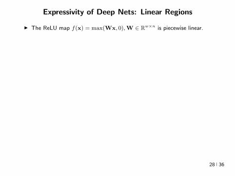
Expressivity of Deep Nets Linear Regions
I The ReLU map f(x) = max(Wx 0)W isin Rwtimesn is piecewise linear
I A piece is a connected region (a convex polytope) of Rd with sharedsparsity pattern in activations
I (Zaslavsky 1975) Number of linear regions formed by an arrangement of
s hyperplanes in d-dimensions in general position issumd
i=0
(si
)I Composition of ReLU maps is also piecewise linear
I (Raghu et al 2017 Pascano et al 2014 Montufar 2014) Number oflinear regions grows as O(wnd) for a composition of d ReLU maps(nrarr brarr brarr b rarr b) each of width w
I (Safran and Shamir 2017)
ndash 1[x le 1] x isin Rd ε-accurate 3-layer network with O(dε) neurons but cannot be approximated with
accuracy higher than O(1d4) using 2-layer networks unless width is exponential in d
28 36
Expressivity of Deep Nets Linear Regions
I The ReLU map f(x) = max(Wx 0)W isin Rwtimesn is piecewise linear
I A piece is a connected region (a convex polytope) of Rd with sharedsparsity pattern in activations
I (Zaslavsky 1975) Number of linear regions formed by an arrangement of
s hyperplanes in d-dimensions in general position issumd
i=0
(si
)I Composition of ReLU maps is also piecewise linear
I (Raghu et al 2017 Pascano et al 2014 Montufar 2014) Number oflinear regions grows as O(wnd) for a composition of d ReLU maps(nrarr brarr brarr b rarr b) each of width w
I (Safran and Shamir 2017)
ndash 1[x le 1] x isin Rd ε-accurate 3-layer network with O(dε) neurons but cannot be approximated with
accuracy higher than O(1d4) using 2-layer networks unless width is exponential in d
28 36
Expressivity of Deep Nets Linear Regions
I The ReLU map f(x) = max(Wx 0)W isin Rwtimesn is piecewise linear
I A piece is a connected region (a convex polytope) of Rd with sharedsparsity pattern in activations
I (Zaslavsky 1975) Number of linear regions formed by an arrangement of
s hyperplanes in d-dimensions in general position issumd
i=0
(si
)
I Composition of ReLU maps is also piecewise linear
I (Raghu et al 2017 Pascano et al 2014 Montufar 2014) Number oflinear regions grows as O(wnd) for a composition of d ReLU maps(nrarr brarr brarr b rarr b) each of width w
I (Safran and Shamir 2017)
ndash 1[x le 1] x isin Rd ε-accurate 3-layer network with O(dε) neurons but cannot be approximated with
accuracy higher than O(1d4) using 2-layer networks unless width is exponential in d
28 36
Expressivity of Deep Nets Linear Regions
I The ReLU map f(x) = max(Wx 0)W isin Rwtimesn is piecewise linear
I A piece is a connected region (a convex polytope) of Rd with sharedsparsity pattern in activations
I (Zaslavsky 1975) Number of linear regions formed by an arrangement of
s hyperplanes in d-dimensions in general position issumd
i=0
(si
)I Composition of ReLU maps is also piecewise linear
I (Raghu et al 2017 Pascano et al 2014 Montufar 2014) Number oflinear regions grows as O(wnd) for a composition of d ReLU maps(nrarr brarr brarr b rarr b) each of width w
I (Safran and Shamir 2017)
ndash 1[x le 1] x isin Rd ε-accurate 3-layer network with O(dε) neurons but cannot be approximated with
accuracy higher than O(1d4) using 2-layer networks unless width is exponential in d28 36
Expressivity of Deep Nets Trajectory Length
I (Raghu et al 2017) Trajectory Length (ldquogeneralized operator normrdquo)How much is a curve in the input space stretched by a layer in thenetwork
29 36
Expressivity of Deep Nets Trajectory Length
I (Raghu et al 2017) Trajectory Length (ldquogeneralized operator normrdquo)How much is a curve in the input space stretched by a layer in thenetwork
29 36
Expressivity and Generalization
I Expressiveness equiv capacity to fit random noise =rArr susceptibility tooverfitting (VC dimension Rademacher Complexity)
I Zhang et al 2017 Famous CNNs easily fit random labels
ndash Over-parameterized (n=12M psim 60M) but structuredndash Domain-knowledge baked in does not constraint expressiveness
I CNNs tend to generalize even without regularization (explicit and implicit)
I For linear regression SGD returns minimum norm solution
30 36
Expressivity and Generalization
I Expressiveness equiv capacity to fit random noise =rArr susceptibility tooverfitting (VC dimension Rademacher Complexity)
I Zhang et al 2017 Famous CNNs easily fit random labels
ndash Over-parameterized (n=12M psim 60M) but structuredndash Domain-knowledge baked in does not constraint expressiveness
I CNNs tend to generalize even without regularization (explicit and implicit)
I For linear regression SGD returns minimum norm solution
30 36
Expressivity and Generalization
I Expressiveness equiv capacity to fit random noise =rArr susceptibility tooverfitting (VC dimension Rademacher Complexity)
I Zhang et al 2017 Famous CNNs easily fit random labels
ndash Over-parameterized (n=12M psim 60M) but structuredndash Domain-knowledge baked in does not constraint expressiveness
I CNNs tend to generalize even without regularization (explicit and implicit)
I For linear regression SGD returns minimum norm solution
30 36
Optimization Landscape Symmetry and Saddle Points
I Folklore lots of equivalent good local minI Classification of critical points based on Hessian spectrumI Permutation and Scaling symmetries
I Thm [Lee et al 2016 Anadkumar Ge] For the short-step gradientmethod the basin of attraction of strict saddle points (atleast onenegative eigenvalue) has measure zero
31 36
Optimization Landscape Symmetry and Saddle Points
I Folklore lots of equivalent good local minI Classification of critical points based on Hessian spectrumI Permutation and Scaling symmetries
I Thm [Lee et al 2016 Anadkumar Ge] For the short-step gradientmethod the basin of attraction of strict saddle points (atleast onenegative eigenvalue) has measure zero
31 36
Optimization Landscape Symmetry and Saddle Points
I Folklore lots of equivalent good local minI Classification of critical points based on Hessian spectrumI Permutation and Scaling symmetries
I Thm [Lee et al 2016 Anadkumar Ge] For the short-step gradientmethod the basin of attraction of strict saddle points (atleast onenegative eigenvalue) has measure zero
31 36
Optimization Landscape Sharp Minima and Stability
Keskar et al 2017 On large-batch training for DL Generalization Gap and Sharp Minima
32 36
Deep Learning Computational Graphs TensorFlow
tensorfloworg
I Tensors-in Tensors-out
I Evergrowing list of Tensor-Ops (PythonC++)
f(xw)
[partf
partx
]T v
[partf
partw
]T v
I Automatic Differentiation Reverse mode
partxL
partxi=sumirarrj
partxL
partxj
partxj
partxi
33 36
Computational Graphs and TensorFlow
tensorfloworg
I SGD with minibatches
wk+1 = wk minus ηlsumi=1
partli
partw
∣∣∣wt
I Model Parallelism Assign independent paths tothreads GPUs
I Data Parallelism create Graph replicas on differentmachines
I Mobile TensorFlow
34 36
Computational Graphs and TensorFlow
tensorfloworg
35 36
Computational Graphs and TensorFlow
tensorfloworg
35 36
Computational Graphs and TensorFlow
tensorfloworg
35 36
Challenges and Opportunities
I Lots of fascinating unsolved problems
I Can you win Imagenet with Convex optimization
I Tools from polynomial optimization (global optimization deep-RL)
I Supervised to Semi-supervised to Unsupervised Learning
I Compact efficient real-time models (eliminateover-parametrization) for new form factors
I Exciting emerging world of Robotics Wearable ComputersIntelligent home devices Personal digital assistants
Google Internship Program
36 36
- anm0
- fdrm0
- fdrm5
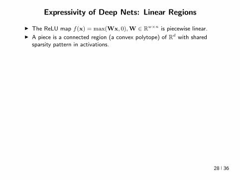
Expressivity of Deep Nets Linear Regions
I The ReLU map f(x) = max(Wx 0)W isin Rwtimesn is piecewise linear
I A piece is a connected region (a convex polytope) of Rd with sharedsparsity pattern in activations
I (Zaslavsky 1975) Number of linear regions formed by an arrangement of
s hyperplanes in d-dimensions in general position issumd
i=0
(si
)I Composition of ReLU maps is also piecewise linear
I (Raghu et al 2017 Pascano et al 2014 Montufar 2014) Number oflinear regions grows as O(wnd) for a composition of d ReLU maps(nrarr brarr brarr b rarr b) each of width w
I (Safran and Shamir 2017)
ndash 1[x le 1] x isin Rd ε-accurate 3-layer network with O(dε) neurons but cannot be approximated with
accuracy higher than O(1d4) using 2-layer networks unless width is exponential in d
28 36
Expressivity of Deep Nets Linear Regions
I The ReLU map f(x) = max(Wx 0)W isin Rwtimesn is piecewise linear
I A piece is a connected region (a convex polytope) of Rd with sharedsparsity pattern in activations
I (Zaslavsky 1975) Number of linear regions formed by an arrangement of
s hyperplanes in d-dimensions in general position issumd
i=0
(si
)
I Composition of ReLU maps is also piecewise linear
I (Raghu et al 2017 Pascano et al 2014 Montufar 2014) Number oflinear regions grows as O(wnd) for a composition of d ReLU maps(nrarr brarr brarr b rarr b) each of width w
I (Safran and Shamir 2017)
ndash 1[x le 1] x isin Rd ε-accurate 3-layer network with O(dε) neurons but cannot be approximated with
accuracy higher than O(1d4) using 2-layer networks unless width is exponential in d
28 36
Expressivity of Deep Nets Linear Regions
I The ReLU map f(x) = max(Wx 0)W isin Rwtimesn is piecewise linear
I A piece is a connected region (a convex polytope) of Rd with sharedsparsity pattern in activations
I (Zaslavsky 1975) Number of linear regions formed by an arrangement of
s hyperplanes in d-dimensions in general position issumd
i=0
(si
)I Composition of ReLU maps is also piecewise linear
I (Raghu et al 2017 Pascano et al 2014 Montufar 2014) Number oflinear regions grows as O(wnd) for a composition of d ReLU maps(nrarr brarr brarr b rarr b) each of width w
I (Safran and Shamir 2017)
ndash 1[x le 1] x isin Rd ε-accurate 3-layer network with O(dε) neurons but cannot be approximated with
accuracy higher than O(1d4) using 2-layer networks unless width is exponential in d28 36
Expressivity of Deep Nets Trajectory Length
I (Raghu et al 2017) Trajectory Length (ldquogeneralized operator normrdquo)How much is a curve in the input space stretched by a layer in thenetwork
29 36
Expressivity of Deep Nets Trajectory Length
I (Raghu et al 2017) Trajectory Length (ldquogeneralized operator normrdquo)How much is a curve in the input space stretched by a layer in thenetwork
29 36
Expressivity and Generalization
I Expressiveness equiv capacity to fit random noise =rArr susceptibility tooverfitting (VC dimension Rademacher Complexity)
I Zhang et al 2017 Famous CNNs easily fit random labels
ndash Over-parameterized (n=12M psim 60M) but structuredndash Domain-knowledge baked in does not constraint expressiveness
I CNNs tend to generalize even without regularization (explicit and implicit)
I For linear regression SGD returns minimum norm solution
30 36
Expressivity and Generalization
I Expressiveness equiv capacity to fit random noise =rArr susceptibility tooverfitting (VC dimension Rademacher Complexity)
I Zhang et al 2017 Famous CNNs easily fit random labels
ndash Over-parameterized (n=12M psim 60M) but structuredndash Domain-knowledge baked in does not constraint expressiveness
I CNNs tend to generalize even without regularization (explicit and implicit)
I For linear regression SGD returns minimum norm solution
30 36
Expressivity and Generalization
I Expressiveness equiv capacity to fit random noise =rArr susceptibility tooverfitting (VC dimension Rademacher Complexity)
I Zhang et al 2017 Famous CNNs easily fit random labels
ndash Over-parameterized (n=12M psim 60M) but structuredndash Domain-knowledge baked in does not constraint expressiveness
I CNNs tend to generalize even without regularization (explicit and implicit)
I For linear regression SGD returns minimum norm solution
30 36
Optimization Landscape Symmetry and Saddle Points
I Folklore lots of equivalent good local minI Classification of critical points based on Hessian spectrumI Permutation and Scaling symmetries
I Thm [Lee et al 2016 Anadkumar Ge] For the short-step gradientmethod the basin of attraction of strict saddle points (atleast onenegative eigenvalue) has measure zero
31 36
Optimization Landscape Symmetry and Saddle Points
I Folklore lots of equivalent good local minI Classification of critical points based on Hessian spectrumI Permutation and Scaling symmetries
I Thm [Lee et al 2016 Anadkumar Ge] For the short-step gradientmethod the basin of attraction of strict saddle points (atleast onenegative eigenvalue) has measure zero
31 36
Optimization Landscape Symmetry and Saddle Points
I Folklore lots of equivalent good local minI Classification of critical points based on Hessian spectrumI Permutation and Scaling symmetries
I Thm [Lee et al 2016 Anadkumar Ge] For the short-step gradientmethod the basin of attraction of strict saddle points (atleast onenegative eigenvalue) has measure zero
31 36
Optimization Landscape Sharp Minima and Stability
Keskar et al 2017 On large-batch training for DL Generalization Gap and Sharp Minima
32 36
Deep Learning Computational Graphs TensorFlow
tensorfloworg
I Tensors-in Tensors-out
I Evergrowing list of Tensor-Ops (PythonC++)
f(xw)
[partf
partx
]T v
[partf
partw
]T v
I Automatic Differentiation Reverse mode
partxL
partxi=sumirarrj
partxL
partxj
partxj
partxi
33 36
Computational Graphs and TensorFlow
tensorfloworg
I SGD with minibatches
wk+1 = wk minus ηlsumi=1
partli
partw
∣∣∣wt
I Model Parallelism Assign independent paths tothreads GPUs
I Data Parallelism create Graph replicas on differentmachines
I Mobile TensorFlow
34 36
Computational Graphs and TensorFlow
tensorfloworg
35 36
Computational Graphs and TensorFlow
tensorfloworg
35 36
Computational Graphs and TensorFlow
tensorfloworg
35 36
Challenges and Opportunities
I Lots of fascinating unsolved problems
I Can you win Imagenet with Convex optimization
I Tools from polynomial optimization (global optimization deep-RL)
I Supervised to Semi-supervised to Unsupervised Learning
I Compact efficient real-time models (eliminateover-parametrization) for new form factors
I Exciting emerging world of Robotics Wearable ComputersIntelligent home devices Personal digital assistants
Google Internship Program
36 36
- anm0
- fdrm0
- fdrm5
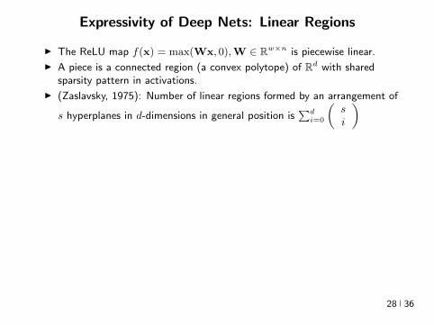
Expressivity of Deep Nets Linear Regions
I The ReLU map f(x) = max(Wx 0)W isin Rwtimesn is piecewise linear
I A piece is a connected region (a convex polytope) of Rd with sharedsparsity pattern in activations
I (Zaslavsky 1975) Number of linear regions formed by an arrangement of
s hyperplanes in d-dimensions in general position issumd
i=0
(si
)I Composition of ReLU maps is also piecewise linear
I (Raghu et al 2017 Pascano et al 2014 Montufar 2014) Number oflinear regions grows as O(wnd) for a composition of d ReLU maps(nrarr brarr brarr b rarr b) each of width w
I (Safran and Shamir 2017)
ndash 1[x le 1] x isin Rd ε-accurate 3-layer network with O(dε) neurons but cannot be approximated with
accuracy higher than O(1d4) using 2-layer networks unless width is exponential in d28 36
Expressivity of Deep Nets Trajectory Length
I (Raghu et al 2017) Trajectory Length (ldquogeneralized operator normrdquo)How much is a curve in the input space stretched by a layer in thenetwork
29 36
Expressivity of Deep Nets Trajectory Length
I (Raghu et al 2017) Trajectory Length (ldquogeneralized operator normrdquo)How much is a curve in the input space stretched by a layer in thenetwork
29 36
Expressivity and Generalization
I Expressiveness equiv capacity to fit random noise =rArr susceptibility tooverfitting (VC dimension Rademacher Complexity)
I Zhang et al 2017 Famous CNNs easily fit random labels
ndash Over-parameterized (n=12M psim 60M) but structuredndash Domain-knowledge baked in does not constraint expressiveness
I CNNs tend to generalize even without regularization (explicit and implicit)
I For linear regression SGD returns minimum norm solution
30 36
Expressivity and Generalization
I Expressiveness equiv capacity to fit random noise =rArr susceptibility tooverfitting (VC dimension Rademacher Complexity)
I Zhang et al 2017 Famous CNNs easily fit random labels
ndash Over-parameterized (n=12M psim 60M) but structuredndash Domain-knowledge baked in does not constraint expressiveness
I CNNs tend to generalize even without regularization (explicit and implicit)
I For linear regression SGD returns minimum norm solution
30 36
Expressivity and Generalization
I Expressiveness equiv capacity to fit random noise =rArr susceptibility tooverfitting (VC dimension Rademacher Complexity)
I Zhang et al 2017 Famous CNNs easily fit random labels
ndash Over-parameterized (n=12M psim 60M) but structuredndash Domain-knowledge baked in does not constraint expressiveness
I CNNs tend to generalize even without regularization (explicit and implicit)
I For linear regression SGD returns minimum norm solution
30 36
Optimization Landscape Symmetry and Saddle Points
I Folklore lots of equivalent good local minI Classification of critical points based on Hessian spectrumI Permutation and Scaling symmetries
I Thm [Lee et al 2016 Anadkumar Ge] For the short-step gradientmethod the basin of attraction of strict saddle points (atleast onenegative eigenvalue) has measure zero
31 36
Optimization Landscape Symmetry and Saddle Points
I Folklore lots of equivalent good local minI Classification of critical points based on Hessian spectrumI Permutation and Scaling symmetries
I Thm [Lee et al 2016 Anadkumar Ge] For the short-step gradientmethod the basin of attraction of strict saddle points (atleast onenegative eigenvalue) has measure zero
31 36
Optimization Landscape Symmetry and Saddle Points
I Folklore lots of equivalent good local minI Classification of critical points based on Hessian spectrumI Permutation and Scaling symmetries
I Thm [Lee et al 2016 Anadkumar Ge] For the short-step gradientmethod the basin of attraction of strict saddle points (atleast onenegative eigenvalue) has measure zero
31 36
Optimization Landscape Sharp Minima and Stability
Keskar et al 2017 On large-batch training for DL Generalization Gap and Sharp Minima
32 36
Deep Learning Computational Graphs TensorFlow
tensorfloworg
I Tensors-in Tensors-out
I Evergrowing list of Tensor-Ops (PythonC++)
f(xw)
[partf
partx
]T v
[partf
partw
]T v
I Automatic Differentiation Reverse mode
partxL
partxi=sumirarrj
partxL
partxj
partxj
partxi
33 36
Computational Graphs and TensorFlow
tensorfloworg
I SGD with minibatches
wk+1 = wk minus ηlsumi=1
partli
partw
∣∣∣wt
I Model Parallelism Assign independent paths tothreads GPUs
I Data Parallelism create Graph replicas on differentmachines
I Mobile TensorFlow
34 36
Computational Graphs and TensorFlow
tensorfloworg
35 36
Computational Graphs and TensorFlow
tensorfloworg
35 36
Computational Graphs and TensorFlow
tensorfloworg
35 36
Challenges and Opportunities
I Lots of fascinating unsolved problems
I Can you win Imagenet with Convex optimization
I Tools from polynomial optimization (global optimization deep-RL)
I Supervised to Semi-supervised to Unsupervised Learning
I Compact efficient real-time models (eliminateover-parametrization) for new form factors
I Exciting emerging world of Robotics Wearable ComputersIntelligent home devices Personal digital assistants
Google Internship Program
36 36
- anm0
- fdrm0
- fdrm5

Expressivity of Deep Nets Trajectory Length
I (Raghu et al 2017) Trajectory Length (ldquogeneralized operator normrdquo)How much is a curve in the input space stretched by a layer in thenetwork
29 36
Expressivity of Deep Nets Trajectory Length
I (Raghu et al 2017) Trajectory Length (ldquogeneralized operator normrdquo)How much is a curve in the input space stretched by a layer in thenetwork
29 36
Expressivity and Generalization
I Expressiveness equiv capacity to fit random noise =rArr susceptibility tooverfitting (VC dimension Rademacher Complexity)
I Zhang et al 2017 Famous CNNs easily fit random labels
ndash Over-parameterized (n=12M psim 60M) but structuredndash Domain-knowledge baked in does not constraint expressiveness
I CNNs tend to generalize even without regularization (explicit and implicit)
I For linear regression SGD returns minimum norm solution
30 36
Optimization Landscape Symmetry and Saddle Points
I Folklore lots of equivalent good local minI Classification of critical points based on Hessian spectrumI Permutation and Scaling symmetries
I Thm [Lee et al 2016 Anadkumar Ge] For the short-step gradientmethod the basin of attraction of strict saddle points (atleast onenegative eigenvalue) has measure zero
31 36
Optimization Landscape Sharp Minima and Stability
Keskar et al 2017 On large-batch training for DL Generalization Gap and Sharp Minima
32 36
Deep Learning Computational Graphs TensorFlow
tensorfloworg
I Tensors-in Tensors-out
I Evergrowing list of Tensor-Ops (PythonC++)
f(xw)
[partf
partx
]T v
[partf
partw
]T v
I Automatic Differentiation Reverse mode
partxL
partxi=sumirarrj
partxL
partxj
partxj
partxi
33 36
Computational Graphs and TensorFlow
tensorfloworg
I SGD with minibatches
wk+1 = wk minus ηlsumi=1
partli
partw
∣∣∣wt
I Model Parallelism Assign independent paths tothreads GPUs
I Data Parallelism create Graph replicas on differentmachines
I Mobile TensorFlow
34 36
Computational Graphs and TensorFlow
tensorfloworg
35 36
Computational Graphs and TensorFlow
tensorfloworg
35 36
Computational Graphs and TensorFlow
tensorfloworg
35 36
Challenges and Opportunities
I Lots of fascinating unsolved problems
I Can you win Imagenet with Convex optimization
I Tools from polynomial optimization (global optimization deep-RL)
I Supervised to Semi-supervised to Unsupervised Learning
I Compact efficient real-time models (eliminateover-parametrization) for new form factors
I Exciting emerging world of Robotics Wearable ComputersIntelligent home devices Personal digital assistants
Google Internship Program
36 36
- anm0
- fdrm0
- fdrm5

Expressivity of Deep Nets Trajectory Length
I (Raghu et al 2017) Trajectory Length (ldquogeneralized operator normrdquo)How much is a curve in the input space stretched by a layer in thenetwork
29 36
Expressivity and Generalization
I Expressiveness equiv capacity to fit random noise =rArr susceptibility tooverfitting (VC dimension Rademacher Complexity)
I Zhang et al 2017 Famous CNNs easily fit random labels
ndash Over-parameterized (n=12M psim 60M) but structuredndash Domain-knowledge baked in does not constraint expressiveness
I CNNs tend to generalize even without regularization (explicit and implicit)
I For linear regression SGD returns minimum norm solution
30 36
Optimization Landscape Symmetry and Saddle Points
I Folklore lots of equivalent good local minI Classification of critical points based on Hessian spectrumI Permutation and Scaling symmetries
I Thm [Lee et al 2016 Anadkumar Ge] For the short-step gradientmethod the basin of attraction of strict saddle points (atleast onenegative eigenvalue) has measure zero
31 36
Optimization Landscape Sharp Minima and Stability
Keskar et al 2017 On large-batch training for DL Generalization Gap and Sharp Minima
32 36
Deep Learning Computational Graphs TensorFlow
tensorfloworg
I Tensors-in Tensors-out
I Evergrowing list of Tensor-Ops (PythonC++)
f(xw)
[partf
partx
]T v
[partf
partw
]T v
I Automatic Differentiation Reverse mode
partxL
partxi=sumirarrj
partxL
partxj
partxj
partxi
33 36
Computational Graphs and TensorFlow
tensorfloworg
I SGD with minibatches
wk+1 = wk minus ηlsumi=1
partli
partw
∣∣∣wt
I Model Parallelism Assign independent paths tothreads GPUs
I Data Parallelism create Graph replicas on differentmachines
I Mobile TensorFlow
34 36
Computational Graphs and TensorFlow
tensorfloworg
35 36
Computational Graphs and TensorFlow
tensorfloworg
35 36
Computational Graphs and TensorFlow
tensorfloworg
35 36
Challenges and Opportunities
I Lots of fascinating unsolved problems
I Can you win Imagenet with Convex optimization
I Tools from polynomial optimization (global optimization deep-RL)
I Supervised to Semi-supervised to Unsupervised Learning
I Compact efficient real-time models (eliminateover-parametrization) for new form factors
I Exciting emerging world of Robotics Wearable ComputersIntelligent home devices Personal digital assistants
Google Internship Program
36 36
- anm0
- fdrm0
- fdrm5

Expressivity and Generalization
I Expressiveness equiv capacity to fit random noise =rArr susceptibility tooverfitting (VC dimension Rademacher Complexity)
I Zhang et al 2017 Famous CNNs easily fit random labels
ndash Over-parameterized (n=12M psim 60M) but structuredndash Domain-knowledge baked in does not constraint expressiveness
I CNNs tend to generalize even without regularization (explicit and implicit)
I For linear regression SGD returns minimum norm solution
30 36
Optimization Landscape Symmetry and Saddle Points
I Folklore lots of equivalent good local minI Classification of critical points based on Hessian spectrumI Permutation and Scaling symmetries
I Thm [Lee et al 2016 Anadkumar Ge] For the short-step gradientmethod the basin of attraction of strict saddle points (atleast onenegative eigenvalue) has measure zero
31 36
Optimization Landscape Sharp Minima and Stability
Keskar et al 2017 On large-batch training for DL Generalization Gap and Sharp Minima
32 36
Deep Learning Computational Graphs TensorFlow
tensorfloworg
I Tensors-in Tensors-out
I Evergrowing list of Tensor-Ops (PythonC++)
f(xw)
[partf
partx
]T v
[partf
partw
]T v
I Automatic Differentiation Reverse mode
partxL
partxi=sumirarrj
partxL
partxj
partxj
partxi
33 36
Computational Graphs and TensorFlow
tensorfloworg
I SGD with minibatches
wk+1 = wk minus ηlsumi=1
partli
partw
∣∣∣wt
I Model Parallelism Assign independent paths tothreads GPUs
I Data Parallelism create Graph replicas on differentmachines
I Mobile TensorFlow
34 36
Computational Graphs and TensorFlow
tensorfloworg
35 36
Computational Graphs and TensorFlow
tensorfloworg
35 36
Computational Graphs and TensorFlow
tensorfloworg
35 36
Challenges and Opportunities
I Lots of fascinating unsolved problems
I Can you win Imagenet with Convex optimization
I Tools from polynomial optimization (global optimization deep-RL)
I Supervised to Semi-supervised to Unsupervised Learning
I Compact efficient real-time models (eliminateover-parametrization) for new form factors
I Exciting emerging world of Robotics Wearable ComputersIntelligent home devices Personal digital assistants
Google Internship Program
36 36
- anm0
- fdrm0
- fdrm5

Expressivity and Generalization
I Expressiveness equiv capacity to fit random noise =rArr susceptibility tooverfitting (VC dimension Rademacher Complexity)
I Zhang et al 2017 Famous CNNs easily fit random labels
ndash Over-parameterized (n=12M psim 60M) but structuredndash Domain-knowledge baked in does not constraint expressiveness
I CNNs tend to generalize even without regularization (explicit and implicit)
I For linear regression SGD returns minimum norm solution
30 36
Expressivity and Generalization
I Expressiveness equiv capacity to fit random noise =rArr susceptibility tooverfitting (VC dimension Rademacher Complexity)
I Zhang et al 2017 Famous CNNs easily fit random labels
ndash Over-parameterized (n=12M psim 60M) but structuredndash Domain-knowledge baked in does not constraint expressiveness
I CNNs tend to generalize even without regularization (explicit and implicit)
I For linear regression SGD returns minimum norm solution
30 36
Optimization Landscape Symmetry and Saddle Points
I Folklore lots of equivalent good local minI Classification of critical points based on Hessian spectrumI Permutation and Scaling symmetries
I Thm [Lee et al 2016 Anadkumar Ge] For the short-step gradientmethod the basin of attraction of strict saddle points (atleast onenegative eigenvalue) has measure zero
31 36
Optimization Landscape Sharp Minima and Stability
Keskar et al 2017 On large-batch training for DL Generalization Gap and Sharp Minima
32 36
Deep Learning Computational Graphs TensorFlow
tensorfloworg
I Tensors-in Tensors-out
I Evergrowing list of Tensor-Ops (PythonC++)
f(xw)
[partf
partx
]T v
[partf
partw
]T v
I Automatic Differentiation Reverse mode
partxL
partxi=sumirarrj
partxL
partxj
partxj
partxi
33 36
Computational Graphs and TensorFlow
tensorfloworg
I SGD with minibatches
wk+1 = wk minus ηlsumi=1
partli
partw
∣∣∣wt
I Model Parallelism Assign independent paths tothreads GPUs
I Data Parallelism create Graph replicas on differentmachines
I Mobile TensorFlow
34 36
Computational Graphs and TensorFlow
tensorfloworg
35 36
Computational Graphs and TensorFlow
tensorfloworg
35 36
Computational Graphs and TensorFlow
tensorfloworg
35 36
Challenges and Opportunities
I Lots of fascinating unsolved problems
I Can you win Imagenet with Convex optimization
I Tools from polynomial optimization (global optimization deep-RL)
I Supervised to Semi-supervised to Unsupervised Learning
I Compact efficient real-time models (eliminateover-parametrization) for new form factors
I Exciting emerging world of Robotics Wearable ComputersIntelligent home devices Personal digital assistants
Google Internship Program
36 36
- anm0
- fdrm0
- fdrm5

Expressivity and Generalization
I Expressiveness equiv capacity to fit random noise =rArr susceptibility tooverfitting (VC dimension Rademacher Complexity)
I Zhang et al 2017 Famous CNNs easily fit random labels
ndash Over-parameterized (n=12M psim 60M) but structuredndash Domain-knowledge baked in does not constraint expressiveness
I CNNs tend to generalize even without regularization (explicit and implicit)
I For linear regression SGD returns minimum norm solution
30 36
Optimization Landscape Symmetry and Saddle Points
I Folklore lots of equivalent good local minI Classification of critical points based on Hessian spectrumI Permutation and Scaling symmetries
I Thm [Lee et al 2016 Anadkumar Ge] For the short-step gradientmethod the basin of attraction of strict saddle points (atleast onenegative eigenvalue) has measure zero
31 36
Optimization Landscape Sharp Minima and Stability
Keskar et al 2017 On large-batch training for DL Generalization Gap and Sharp Minima
32 36
Deep Learning Computational Graphs TensorFlow
tensorfloworg
I Tensors-in Tensors-out
I Evergrowing list of Tensor-Ops (PythonC++)
f(xw)
[partf
partx
]T v
[partf
partw
]T v
I Automatic Differentiation Reverse mode
partxL
partxi=sumirarrj
partxL
partxj
partxj
partxi
33 36
Computational Graphs and TensorFlow
tensorfloworg
I SGD with minibatches
wk+1 = wk minus ηlsumi=1
partli
partw
∣∣∣wt
I Model Parallelism Assign independent paths tothreads GPUs
I Data Parallelism create Graph replicas on differentmachines
I Mobile TensorFlow
34 36
Computational Graphs and TensorFlow
tensorfloworg
35 36
Computational Graphs and TensorFlow
tensorfloworg
35 36
Computational Graphs and TensorFlow
tensorfloworg
35 36
Challenges and Opportunities
I Lots of fascinating unsolved problems
I Can you win Imagenet with Convex optimization
I Tools from polynomial optimization (global optimization deep-RL)
I Supervised to Semi-supervised to Unsupervised Learning
I Compact efficient real-time models (eliminateover-parametrization) for new form factors
I Exciting emerging world of Robotics Wearable ComputersIntelligent home devices Personal digital assistants
Google Internship Program
36 36
- anm0
- fdrm0
- fdrm5

Optimization Landscape Symmetry and Saddle Points
I Folklore lots of equivalent good local minI Classification of critical points based on Hessian spectrumI Permutation and Scaling symmetries
I Thm [Lee et al 2016 Anadkumar Ge] For the short-step gradientmethod the basin of attraction of strict saddle points (atleast onenegative eigenvalue) has measure zero
31 36
Optimization Landscape Sharp Minima and Stability
Keskar et al 2017 On large-batch training for DL Generalization Gap and Sharp Minima
32 36
Deep Learning Computational Graphs TensorFlow
tensorfloworg
I Tensors-in Tensors-out
I Evergrowing list of Tensor-Ops (PythonC++)
f(xw)
[partf
partx
]T v
[partf
partw
]T v
I Automatic Differentiation Reverse mode
partxL
partxi=sumirarrj
partxL
partxj
partxj
partxi
33 36
Computational Graphs and TensorFlow
tensorfloworg
I SGD with minibatches
wk+1 = wk minus ηlsumi=1
partli
partw
∣∣∣wt
I Model Parallelism Assign independent paths tothreads GPUs
I Data Parallelism create Graph replicas on differentmachines
I Mobile TensorFlow
34 36
Computational Graphs and TensorFlow
tensorfloworg
35 36
Computational Graphs and TensorFlow
tensorfloworg
35 36
Computational Graphs and TensorFlow
tensorfloworg
35 36
Challenges and Opportunities
I Lots of fascinating unsolved problems
I Can you win Imagenet with Convex optimization
I Tools from polynomial optimization (global optimization deep-RL)
I Supervised to Semi-supervised to Unsupervised Learning
I Compact efficient real-time models (eliminateover-parametrization) for new form factors
I Exciting emerging world of Robotics Wearable ComputersIntelligent home devices Personal digital assistants
Google Internship Program
36 36
- anm0
- fdrm0
- fdrm5

Optimization Landscape Symmetry and Saddle Points
I Folklore lots of equivalent good local minI Classification of critical points based on Hessian spectrumI Permutation and Scaling symmetries
I Thm [Lee et al 2016 Anadkumar Ge] For the short-step gradientmethod the basin of attraction of strict saddle points (atleast onenegative eigenvalue) has measure zero
31 36
Optimization Landscape Symmetry and Saddle Points
I Folklore lots of equivalent good local minI Classification of critical points based on Hessian spectrumI Permutation and Scaling symmetries
I Thm [Lee et al 2016 Anadkumar Ge] For the short-step gradientmethod the basin of attraction of strict saddle points (atleast onenegative eigenvalue) has measure zero
31 36
Optimization Landscape Sharp Minima and Stability
Keskar et al 2017 On large-batch training for DL Generalization Gap and Sharp Minima
32 36
Deep Learning Computational Graphs TensorFlow
tensorfloworg
I Tensors-in Tensors-out
I Evergrowing list of Tensor-Ops (PythonC++)
f(xw)
[partf
partx
]T v
[partf
partw
]T v
I Automatic Differentiation Reverse mode
partxL
partxi=sumirarrj
partxL
partxj
partxj
partxi
33 36
Computational Graphs and TensorFlow
tensorfloworg
I SGD with minibatches
wk+1 = wk minus ηlsumi=1
partli
partw
∣∣∣wt
I Model Parallelism Assign independent paths tothreads GPUs
I Data Parallelism create Graph replicas on differentmachines
I Mobile TensorFlow
34 36
Computational Graphs and TensorFlow
tensorfloworg
35 36
Computational Graphs and TensorFlow
tensorfloworg
35 36
Computational Graphs and TensorFlow
tensorfloworg
35 36
Challenges and Opportunities
I Lots of fascinating unsolved problems
I Can you win Imagenet with Convex optimization
I Tools from polynomial optimization (global optimization deep-RL)
I Supervised to Semi-supervised to Unsupervised Learning
I Compact efficient real-time models (eliminateover-parametrization) for new form factors
I Exciting emerging world of Robotics Wearable ComputersIntelligent home devices Personal digital assistants
Google Internship Program
36 36
- anm0
- fdrm0
- fdrm5

Optimization Landscape Symmetry and Saddle Points
I Folklore lots of equivalent good local minI Classification of critical points based on Hessian spectrumI Permutation and Scaling symmetries
I Thm [Lee et al 2016 Anadkumar Ge] For the short-step gradientmethod the basin of attraction of strict saddle points (atleast onenegative eigenvalue) has measure zero
31 36
Optimization Landscape Sharp Minima and Stability
Keskar et al 2017 On large-batch training for DL Generalization Gap and Sharp Minima
32 36
Deep Learning Computational Graphs TensorFlow
tensorfloworg
I Tensors-in Tensors-out
I Evergrowing list of Tensor-Ops (PythonC++)
f(xw)
[partf
partx
]T v
[partf
partw
]T v
I Automatic Differentiation Reverse mode
partxL
partxi=sumirarrj
partxL
partxj
partxj
partxi
33 36
Computational Graphs and TensorFlow
tensorfloworg
I SGD with minibatches
wk+1 = wk minus ηlsumi=1
partli
partw
∣∣∣wt
I Model Parallelism Assign independent paths tothreads GPUs
I Data Parallelism create Graph replicas on differentmachines
I Mobile TensorFlow
34 36
Computational Graphs and TensorFlow
tensorfloworg
35 36
Computational Graphs and TensorFlow
tensorfloworg
35 36
Computational Graphs and TensorFlow
tensorfloworg
35 36
Challenges and Opportunities
I Lots of fascinating unsolved problems
I Can you win Imagenet with Convex optimization
I Tools from polynomial optimization (global optimization deep-RL)
I Supervised to Semi-supervised to Unsupervised Learning
I Compact efficient real-time models (eliminateover-parametrization) for new form factors
I Exciting emerging world of Robotics Wearable ComputersIntelligent home devices Personal digital assistants
Google Internship Program
36 36
- anm0
- fdrm0
- fdrm5
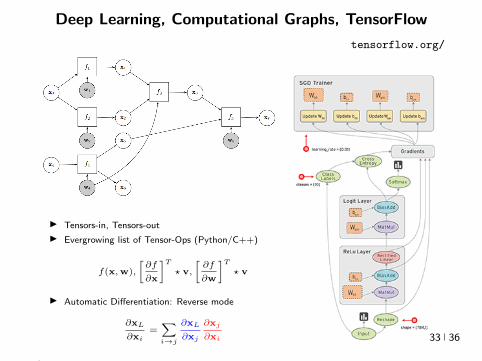
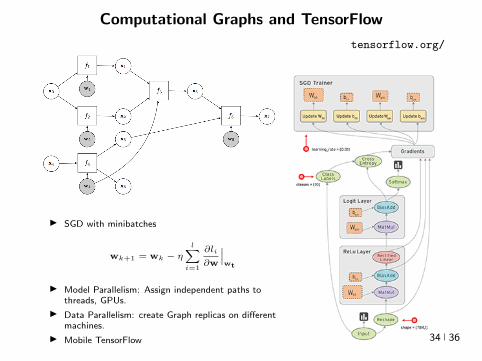
Computational Graphs and TensorFlow
tensorfloworg
I SGD with minibatches
wk+1 = wk minus ηlsumi=1
partli
partw
∣∣∣wt
I Model Parallelism Assign independent paths tothreads GPUs
I Data Parallelism create Graph replicas on differentmachines
I Mobile TensorFlow
34 36
Computational Graphs and TensorFlow
tensorfloworg
35 36
Computational Graphs and TensorFlow
tensorfloworg
35 36
Computational Graphs and TensorFlow
tensorfloworg
35 36
Challenges and Opportunities
I Lots of fascinating unsolved problems
I Can you win Imagenet with Convex optimization
I Tools from polynomial optimization (global optimization deep-RL)
I Supervised to Semi-supervised to Unsupervised Learning
I Compact efficient real-time models (eliminateover-parametrization) for new form factors
I Exciting emerging world of Robotics Wearable ComputersIntelligent home devices Personal digital assistants
Google Internship Program
36 36
- anm0
- fdrm0
- fdrm5
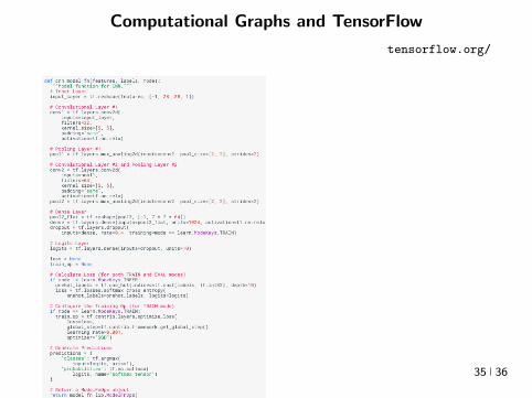
Computational Graphs and TensorFlow
tensorfloworg
35 36
Computational Graphs and TensorFlow
tensorfloworg
35 36
Computational Graphs and TensorFlow
tensorfloworg
35 36
Challenges and Opportunities
I Lots of fascinating unsolved problems
I Can you win Imagenet with Convex optimization
I Tools from polynomial optimization (global optimization deep-RL)
I Supervised to Semi-supervised to Unsupervised Learning
I Compact efficient real-time models (eliminateover-parametrization) for new form factors
I Exciting emerging world of Robotics Wearable ComputersIntelligent home devices Personal digital assistants
Google Internship Program
36 36
- anm0
- fdrm0
- fdrm5

Computational Graphs and TensorFlow
tensorfloworg
35 36
Computational Graphs and TensorFlow
tensorfloworg
35 36
Challenges and Opportunities
I Lots of fascinating unsolved problems
I Can you win Imagenet with Convex optimization
I Tools from polynomial optimization (global optimization deep-RL)
I Supervised to Semi-supervised to Unsupervised Learning
I Compact efficient real-time models (eliminateover-parametrization) for new form factors
I Exciting emerging world of Robotics Wearable ComputersIntelligent home devices Personal digital assistants
Google Internship Program
36 36
- anm0
- fdrm0
- fdrm5
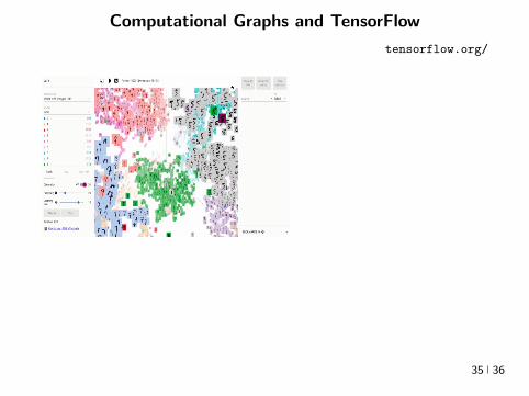
Computational Graphs and TensorFlow
tensorfloworg
35 36
Challenges and Opportunities
I Lots of fascinating unsolved problems
I Can you win Imagenet with Convex optimization
I Tools from polynomial optimization (global optimization deep-RL)
I Supervised to Semi-supervised to Unsupervised Learning
I Compact efficient real-time models (eliminateover-parametrization) for new form factors
I Exciting emerging world of Robotics Wearable ComputersIntelligent home devices Personal digital assistants
Google Internship Program
36 36
- anm0
- fdrm0
- fdrm5