SHEAVES, STACKS, AND SHTUKAS

KIRAN S. KEDLAYA

These are extended notes from a four-lecture series at the 2017 Arizona Winter Schoolon the topic of perfectoid spaces. The appendix describes the proposed student projects(including contributions from David Hansen and Sean Howe). See the table of contentsbelow for a list of topics covered.

These notes have been deliberately written to include much more material than couldpossibly be presented in four one-hour lectures. Certain material (including the definition ofan analytic Huber ring and the extension of various basic results from Tate rings to analyticrings) is original to these notes.

These notes have benefited tremendously from detailed feedback from a number of people,including Bastian Haase, David Hansen, Sean Howe, Shizhang Li, Peter Scholze, and AlexYoucis. In addition, special thanks are due to the participants of the UCSD winter 2017reading seminar on perfectoid spaces: Annie Carter, Zonglin Jiang, Jake Postema, DanielSmith, Claus Sorensen, Xin Tong, and Peter Wear.

Convention 0.0.1. Throughout these lecture notes, the following conventions are in forceunless specifically overridden.

• All rings are commutative and unital.• A complete topological space is required to be Hausdorff (as usual).• All Huber rings and pairs we consider are complete. (This is not the convention usedin [163, Lecture 1].)

Contents

1. Sheaves on analytic adic spaces 31.1. Analytic rings and the open mapping theorem 31.2. The structure sheaf 81.3. Cohomology of sheaves 131.4. Vector bundles and pseudocoherent sheaves 131.5. Huber versus Banach rings 171.6. A strategy of proof: variations on Tate’s reduction 231.7. Proofs: sheafiness 291.8. Proofs: acyclicity 301.9. Proofs: vector bundles and pseudocoherent sheaves 311.10. Remarks on the etale topology 391.11. Preadic spaces 402. Perfectoid rings and spaces 422.1. Perfectoid rings and pairs 422.2. Witt vectors 44

Date: 10 Mar 2017—official AWS version.1

2.3. Tilting and untilting 462.4. Algebraic aspects of tilting 502.5. Geometric aspects of tilting 522.6. Euclidean division for primitive ideals 552.7. Primitive ideals and tilting 582.8. More proofs 602.9. Additional results about perfectoid rings 643. Sheaves on Fargues–Fontaine curves 663.1. Absolute and relative Fargues–Fontaine curves 663.2. An analogy: vector bundles on Riemann surfaces 703.3. The formalism of slopes 723.4. Harder–Narasimhan filtrations 733.5. Additional examples of the slope formalism 783.6. Slopes over a point 823.7. Slopes in families 863.8. More on exotic topologies 884. Shtukas 914.1. Fundamental groups 914.2. Drinfeld’s lemma 994.3. Drinfeld’s lemma for diamonds 1034.4. Shtukas in positive characteristic 1104.5. Shtukas in mixed characteristic 1114.6. Affine Grassmannians 115Appendix A. Project descriptions 118A.1. Extensions of vector bundles and slopes (proposed by David Hansen) 118A.2. G-bundles 118A.3. The open mapping theorem for analytic rings 119A.4. The archimedean Fargues–Fontaine curve (proposed by Sean Howe) 120A.5. Finitely presented morphisms 121A.6. Additional suggestions 121References 122

2

1. Sheaves on analytic adic spaces

We begin by picking up where the first lecture of Weinstein [163, Lecture 1], on theadic spectrum associated to a Huber pair, leaves off. We collect the basic facts we needabout the structure sheaf, vector bundles, and coherent sheaves on the adic spectrum. Theapproach is in some sense motivated by the analogy between the theories of “varieties”(here meaning schemes locally of finite type over a field) and of general schemes. In ourversion of this analogy, the building blocks of the finite-type case are affinoid algebras overa nonarchimedean field (with which we assume some familiarity, e.g., at the level of [21] or[64]), and we are trying to extend to more general Huber rings in order to capture examplesthat are very much not of finite type (notably perfectoid rings). However, this passage doesnot go quite as smoothly as in the theory of schemes, so some care is required to assemble atheory that is both expansive enough to include perfectoid rings, but robust enough to allowus to assert the general theorems we will need.

In order to streamline the exposition, we have opted to state most of the key theorems firstwithout proof (see §1.2–1.4). We then follow with discussion of the overall strategy of proof ofthese theorems (see §1.6), and finally treat the technical details of the proofs (see §1.7–1.9).Along the way, we include some technical subsections that can be skimmed or skipped onfirst reading: one on the open mapping theorem (§1.1), one on Banach rings (§1.5), one onthe etale topology (§1.10), and one on preadic spaces (§1.11).

Hypothesis 1.0.1. Throughout §1, let (A,A+) be a fixed Huber pair (with A complete,as per our conventions) and put X := Spa(A,A+). Unless otherwise specified, we assumealso that A is analytic (see Definition 1.1.2); however, there is little harm done if the readerprefers to assume in addition that A is Tate (see Definition 1.1.2 and Remark 1.1.5).

1.1. Analytic rings and the open mapping theorem. We begin with a brief technicaldiscussion, which can mostly be skipped on first reading. This has to do with the fact thatHuber’s theory of adic spaces includes the theory of formal schemes as a subcase, but we areprimarily interested in the complementary subcase.

Remark 1.1.1. In any Huber ring, the set of units is open: if x is a unit and y is sufficientlyclose to x, then x−1(x− y) is topologically nilpotent and its powers sum to an inverse of y.This implies that any maximal ideal is closed.

This observation is often used in conjunction with [85, Proposition 3.6(i)]: if A 6= 0, thenX 6= ∅. For a derivation of this result, see Corollary 1.5.18.

Definition 1.1.2. Recall that the Huber ring A is said to be Tate (or sometimes microbial)if it contains a topologically nilpotent unit (occasionally called a microbe by analogy withterminology used in real algebraic geometry [47]; more commonly a pseudouniformizer).

More generally, we say that A is analytic if its topologically nilpotent elements generatethe trivial ideal in A; Example 1.5.7 separates these two conditions. The term analytic isnot standard (yet), but is motivated by Lemma 1.1.3 below. By convention, the zero ring isboth Tate and analytic.

We say that a Huber pair (A,A+) is Tate (resp. analytic) if A is Tate (resp. analytic).

Lemma 1.1.3. The following conditions on a general Huber pair (A,A+) are equivalent.(a) The ring A is analytic.(b) Any ideal of definition in any ring of definition generates the unit ideal in A.

3

(c) Every open ideal of A is trivial.(d) For every nontrivial ideal I of A, the quotient topology on A/I is not discrete.(e) The only discrete topological A-module is the zero module.(f) The set X contains no point on whose residue field the induced valuation is trivial.

Proof. We start with some easy implications:• (b) implies (a) (any ideal of definition consists of topologically nilpotent elements);• (b) and (c) are equivalent (any ideal of definition is open, and any open ideal containsan ideal of definition);• (c) and (d) are equivalent (trivially);• (e) implies (d) (trivially).

We next check that (a) implies (b). Suppose that A is analytic, A0 is a ring of definition,and I is an ideal of definition. For any topologically nilpotent elements x1, . . . , xn ∈ A whichgenerate the unit ideal, for any sufficiently large m the elements xm1 , . . . , xmn belong to I andstill generate the unit ideal in A.

At this point, we have the equivalence among (a)–(d). To add (e), we need only checkthat (c) implies (e), which we achieve by checking the contrapositive. Let M be a nonzerodiscrete topological A-module, and choose any nonzero m ∈M . The map A→M , a 7→ amis continuous; its kernel is a nontrivial open ideal of A.

We next check that (a) implies (f). If A is analytic, then for each v ∈ X, we can find atopologically nilpotent element x ∈ A with v(x) 6= 0. We must then have 0 < v(x) < 1, sothe induced valuation on the residue field is nontrivial.

We finally check that (f) implies (d), by establishing the contrapositive. Let I be a nontriv-ial ideal of A such that A/I is discrete for the quotient topology. Then the trivial valuationon the residue field of any maximal ideal of A/I gives rise to a point of X on whose residuefield the induced valuation is trivial.

Corollary 1.1.4. If (A,A+) is an analytic Huber pair, then Spa(A,A+)→ Spa(A+, A+) isinjective. (We will show later that it is also a homeomorphism onto its image; see Lemma 1.6.5.)

Proof. For v ∈ Spa(A,A+), by Lemma 1.1.3 there exists a topologically nilpotent element xof A such that 0 < v(x) < 1. For w ∈ Spa(A,A+) agreeing with v on A+, for any y, z ∈ A,any sufficiently large positive integer n has the property that xny, xnz ∈ A+; it follows thatthe order relations in the pairs

(v(y), v(z)), (v(xny), v(xnz)), (w(xny), w(xnz)), (w(y), w(z))

all coincide, yielding v = w.

Remark 1.1.5. Lemma 1.1.3 shows that a Huber pair (A,A+) is analytic if and only ifSpa(A,A+) is analytic in the sense of Huber. It also shows that if (A,A+) is analytic, thenSpa(A,A+) is covered by rational subspaces (see Definition 1.2.1) which are the adic spectraof Tate rings. Consequently, from the point of view of adic spaces, escalating the level ofgenerality of Huber pairs from Tate to analytic does not create any new geometric objects.However, it does improve various statements about acyclicity of sheaves, as in the rest ofthis lecture.

Exercise 1.1.6. Let A be a Huber ring. If there exists a finite, faithfully flat morphismA→ B such that B is Tate (resp. analytic) under its natural topology as an A-module (seeDefinition 1.1.11), then A is Tate (resp. analytic).

4

Exercise 1.1.7. A (continuous) morphism f : A → B of general Huber rings is adic ifone can choose rings of definition A0, B0 of A,B and an ideal of definition A such thatf(A0) ⊆ B0 and f(I)B0 is an ideal of definition of B0. Prove that this condition is alwayssatisfied when A is analytic.

From now on, assume (unless otherwise indicated) that A is analytic. In the classicaltheory of Banach spaces, the open mapping theorem of Banach plays a fundamental role inshowing that topological properties are often controlled by algebraic properties. The sametheorem is available in the nonarchimedean setting for analytic rings.

Definition 1.1.8. A morphism of topological abelian groups is strict if the subspace andquotient topologies on its image coincide. For a surjective morphism, this is equivalent tothe map being open.

Theorem 1.1.9 (Open mapping theorem). Let f : M → N be a continuous morphism oftopological A-modules which are Hausdorff, first-countable (i.e., 0 admits a countable neigh-borhood basis), and complete (which implies Hausdorff). If f is surjective, then f is open.(Note that A itself is first-countable.)

Proof. As in the archimedean case, this comes down to an application of Baire’s theoremthat every complete metric space is a Baire space (i.e., the union of countably many nowheredense subsets is never open). The case where A is a nonarchimedean field can be treatedin parallel with the archimedean case, as in Bourbaki [23, I.3.3, Theoreme 1]; see also [141,Proposition 8.6]. It was observed by Huber [86, Lemma 2.4(i)] that the argument carriesover to the case where A is Tate; this was made explicit by Henkel [83]. The analytic case issimilar; see Problem A.3.1.

Remark 1.1.10. Theorem 1.1.9 is in fact a characterization of analytic Huber rings: if Ais not analytic, there exists a morphism f : M → N of complete first-countable topologicalA-modules which is continuous but not open. For example, let I be a nontrivial open idealand take M,N to be two copies of

∏n∈Z(A/I) equipped with the discrete topology and the

product topology, respectively. (Thanks to Zonglin Jiang for this example.)

Before stating an immediate corollary of Theorem 1.1.9, we need a definition.

Definition 1.1.11. Let M be a finitely generated A-module. For any A-linear surjectivemorphism F → M , we may form the quotient topology of M ; the resulting topology doesnot depend on the choice. (It suffices to compare with a second surjection F ⊕ F ′ → M byfactoring the map F ′ →M through F ⊕F ′.) This topology is called the natural topology onA.

If A is noetherian, thenM is always complete for its natural topology (see Corollary 1.1.15below). In general, M need not be complete for the natural topology, but the only wayfor completeness to fail is for M to fail to be Hausdorff. Namely, if M is Hausdorff, thenker(F →M) is closed, so quotienting by it gives a complete A-module.

Even ifM is complete for its topology, that does not mean that its image under a morphismof finitely generated A-modules must be complete (unless A is noetherian). For example,for f ∈ A, it can happen that ×f : A → A is injective but its image is not closed; seeRemark 1.8.4.

5

Corollary 1.1.12. Suppose that A is analytic. Let M be a finitely generated A-module. IfM admits the structure of a complete first-countable topological A-module for some topology,then that topology must be the natural topology.

Proof. Apply Theorem 1.1.9 to an A-linear surjection F →M with F finite free.

Let us now see some examples of this theorem in action. The following argument is essen-tially [22, Proposition 3.7.2/1] or [64, Lemma 1.2.3].

Lemma 1.1.13. Let M be a finitely generated A-module which is complete for the naturaltopology. Then any dense A-submodule ofM equalsM itself. (This argument does not requireA to be analytic, but the following corollary does.)

Proof. We may lift the problem to the case whereM is free on the basis e1, . . . , en. Let N bea dense submodule of M ; we may then choose e′1, . . . , e

′n ∈ N such that e′j =

∑iBijei with

Bij being topologically nilpotent if i 6= j and Bii − 1 being topologically nilpotent if i = j.Then the matrix B is invertible (its determinant equals 1 plus a topological nilpotent), soN = M .

Corollary 1.1.14. Let M be a finitely generated A-module which is complete for the naturaltopology. Then any A-submodule of M whose closure is finitely generated is itself closed.

Proof. Let N be an A-submodule whose closure N is finitely generated. By Corollary 1.1.12,the subspace topology on N coincides with the natural topology, so Lemma 1.1.13 may beapplied to see that N = N .

Corollary 1.1.15. The following statements hold.(a) If A is noetherian, then every finitely generated A-module is complete for the natural

topology, and every submodule of such a module is closed.(b) Conversely, if every ideal of A is closed, then A is noetherian.

Proof. Suppose first that A is noetherian. For M a finitely generated A-module and F →Man A-linear surjection with F finite free, Corollary 1.1.14 implies that ker(F →M) is closed,so M is complete. Applying Corollary 1.1.14 again shows that every submodule of M isclosed, yielding (a).

Conversely, suppose that every ideal of A is closed. To prove (b), we will obtain a con-tradiction under the hypothesis that there exists an ascending chain of ideals I1 ⊆ I2 ⊆ · · ·which does not stabilize, by showing that the union I of the chain is not closed. In fact thisalready follows from Baire’s theorem, but we give a more elementary argument below.

Since A is analytic, we can find some finite set x1, . . . , xn of topologically nilpotent unitswhich generate the unit ideal in A. For each m, choose an element ym ∈ Im − Im−1. We canthen choose an index im ∈ 1, . . . , n such that xjimym /∈ Im−1 for all positive integers j.

Let V1, V2, . . . be a cofinal sequence of neighborhoods of 0 in A. We now choose positiveintegers j1, j2, . . . subject to the following conditions (by choosing jm sufficiently large giventhe choice of j1, . . . , jm−1).

(a) For each positive integer m, xjmimym ∈ Vm.(b) For each positive integerm, there exists an open subgroup Um of A such that (xjmimym+

Um) ∩ Im−1 = 0 and xjm′im′ym′ ∈ Um for all m′ > m.

6

Then∑∞

m=1 xjmimym converges to a limit y which is in the closure of I by (a), but not in I by

(b) (for each m we have y ∈ Im−1 + xjmim + Um and hence y /∈ Im−1), a contradiction.

As a concrete example of what happens when A is not noetherian, we offer the followingexercise.

Definition 1.1.16. For A a Huber ring, let A〈T 〉 be the completion of A[T ] for the topologywith a neighborhood basis given by U [T ] =

∑∞n=0 anT

n : an ∈ U for all n as U runsover neighborhoods of 0 in A. We may similarly define A〈T1, . . . , Tm〉, or even the analoguewith infinitely many variables. When the topology on A is induced by a norm, this can beinterpreted in terms of a Gauss1 norm; see Definition 1.5.3.

Exercise 1.1.17. Let p be a prime. Let A be the quotient of the infinite Tate algebraQp〈T, U1, V1, U2, V2, . . . 〉 by the closure of the ideal (TU1 − pV1, TU2 − p2V2, . . . ).

(a) Show that A is uniform (see Definition 1.2.12).(b) Show that T is not a zero-divisor in A.(c) Show that the ideal TA is not closed in A.

The following argument can be found in [86, II.1], [87, Lemma 1.7.6].

Lemma 1.1.18. Let M be an A-module which is the cokernel of a strict morphism betweenfinite projective A-modules. Equivalently by Theorem 1.1.9, M is finitely presented and com-plete for the natural topology.

(a) LetM〈T 〉 be the set of formal sums∑∞

n=0 xnTn with xn ∈M forming a null sequence.

Then the natural map M ⊗A A〈T 〉 →M〈T 〉 is an isomorphism.(b) LetM〈T±〉 be the set of formal sums

∑n∈Z xnT

n with xn ∈M forming a null sequencein each direction. Then the natural map M ⊗AA〈T±〉 →M〈T±〉 is an isomorphism.

Proof. We treat only (a), since (b) is similar. If M is finitely generated and complete for thenatural topology, then it is apparent that M ⊗A A〈T 〉 → M〈T 〉 is surjective. Suppose nowthat as in the statement of the lemma, M is the cokernel of a strict morphism F1 → F0

between finite projective A-modules. Put N := ker(F0 → M); then N is finitely generatedand complete for the natural topology. We thus have a commutative diagram

N ⊗A A〈T 〉 //

F0 ⊗A A〈T 〉 //

M ⊗A A〈T 〉 //

0

0 // N〈T 〉 // F 〈T 〉 // M〈T 〉 // 0

with exact rows in which the middle vertical arrow is an isomorphism and both vertical arrowsare surjective. By the five lemma, it follows that the right vertical arrow is injective.

Lemma 1.1.19. Suppose that A is noetherian.(a) The homomorphism A→ A〈T 〉 is flat.(b) If A〈T 〉 is also noetherian, then A[T ]→ A〈T 〉 is also flat.

1Correctly spelled “Gauß”, but I’ll stick to the customary English transliteration.7

Proof. Let 0 → M → N → P → 0 be an exact sequence of finite A-modules; by Corol-lary 1.1.15, it is also a strict exact sequence for the natural topologies. Consequently, theexact sequence

0→M〈T 〉 → N〈T 〉 → P 〈T 〉 → 0

is the base extension of the previous sequence from A to A〈T 〉. This proves (a).Suppose now that A〈T 〉 is noetherian. To prove (b), by [152, Tag 00MP] it suffices to

check that for every prime ideal p of A, the map A[T ] ⊗A κ(p) → A〈T 〉 ⊗A κ(p) is flat.Since A〈T 〉 is noetherian (and analytic because A is), Corollary 1.1.15 implies that pA〈T 〉is a closed ideal; we may thus identify pA〈T 〉 with the subset p〈T 〉 of A〈T 〉 (again as inLemma 1.1.18. In particular, as a module over the principal ideal domain A[T ] ⊗A κ(p) =κ(p)[T ], A〈T 〉 ⊗A κ(p) = A〈T 〉/p〈T 〉 is torsion-free and hence flat.

1.2. The structure sheaf. We continue with the definition and analysis of the structurepresheaf. As in the theory of affine schemes, we have in mind a formula for certain distin-guished open subsets, in this case the rational subspaces; the shape of the general definitionis meant to enforce this formula. However, we will almost immediately hit a serious difficultywhich echoes throughout the entire theory.

We recall some facts about rational subsets of X from the previous lecture [163, Lecture 1].

Definition 1.2.1. A rational subspace of X is one of the form

X

(f1, . . . , fn

g

):= v ∈ X : v(fi) ≤ v(g) 6= 0 (i = 1, . . . , n)

where f1, . . . , fn, g ∈ A are some elements which generate an open ideal in A; such subspacesform a neighborhood basis in X. Since we are assuming that A is analytic, by Lemma 1.1.3any open ideal is in fact the trivial ideal; in particular, we may rewrite the previous formulaas

X

(f1, . . . , fn

g

):= v ∈ X : v(fi) ≤ v(g) (i = 1, . . . , n).

There is a morphism (A,A+) → (B,B+) of (complete) Huber pairs which is initial amongmorphisms for which Spa(B,B+) maps into X

(f1,...,fn

g

); this morphism induces a map

Spa(B,B+) ∼= X(f1,...,fn

g

)which not only is a homeomorphism, but matches up rational

subspace of Spa(B,B+) with rational subspaces of X contained in X(f1,...,fn

g

). We call any

such morphism “the” rational localization corresponding to X(f1,...,fn

g

), using the definite

article since the morphism is unique up to unique isomorphism.Since f1, . . . , fn, g generate the unit ideal, the ring B in the pair (B,B+) may be identified

explicitly as the quotient of A〈T1, . . . , Tn〉 by the closure of the ideal (gT1−f1, . . . , gTn−fn);we denote this ring by A

⟨f1,...,fn

g

⟩. (We will see later that when the structure presheaf on X

is a presheaf, it is not necessarily to take the closure; see Theorem 1.2.7.) The ring B+ maybe identified as the integral closure of the image of A+〈T1, . . . , Tn〉 in B; we denote this ringby A+

⟨f1,...,fn

g

⟩.

Exercise 1.2.2. Given f1, . . . , fn, g ∈ A which generate the unit ideal, there exists a neigh-borhoodW of 0 in A such that any f ′1, . . . , f ′n, g′ ∈ A satisfying f ′1−f1, . . . , f

′n−fn, g′−g ∈ W

8

generate the unit ideal and define the same rational subspace as do f1, . . . , fn, g. (See [142,Remark 2.8], [107, Remark 2.4.7].)

Definition 1.2.3. Define the structure presheaf O on X as follows: for U ⊆ X open,let O(U) be the inverse limit of B over all rational localizations (A,A+) → (B,B+) withSpa(B,B+) ⊆ U . In particular, if U = Spa(B,B+) then O(U) = B.

Let O+ be the subsheaf of O defined as follows: for U ⊆ X open, let O(U) be theinverse limit of B+ over all rational localizations (A,A+)→ (B,B+) with Spa(B,B+) ⊆ U .Equivalently,

O+(U) = f ∈ O(U) : v(f) ≤ 1 for all v ∈ U.In particular, if U = Spa(B,B+) then O(U) = B+.

Remark 1.2.4. For any open subset U of X, the ring O(U) is complete for the inverse limittopology, but in general it is not a Huber ring. A typical example is the open unit disc insidethe closed unit disc, which is Frechet complete with respect to the supremum norms over allof the closed discs around the origin of radii less than 1. (This ring cannot be Huber becausethe topologically nilpotent elements do not form an open set.)

Remark 1.2.5. For each x ∈ X, the stalk OX,x is a direct limit of complete rings, and henceis a henselian local ring; in particular, the categories of finite etale algebras over OX,x andover its residue field are equivalent. Compare [107, Lemma 2.4.17].

Remark 1.2.6. In order to follow the theory of affine schemes, one would next expect toprove that the presheaf O is a sheaf. This is indeed true when A is an affinoid algebra overa nonarchimedean field, as this follows (after a small formal argument; see Lemma 1.6.3)from Tate’s acyclicity theorem in rigid analytic geometry [155, Theorem 8.2], [22, Theo-rem 8.2.1/1].

Unfortunately, there exist examples where O is not a sheaf. This remains true if we assumethat A is Tate, as shown by an example of Huber [86, §1]; or even if we assume that A isTate and uniform, as shown by examples of Buzzard–Verberkmoes [25, Proposition 18] andMihara [126, Theorem 3.15].

A conceptual explanation for the previous examples is given by the following result.

Theorem 1.2.7 (original). Suppose that O is a sheaf. Then for any f1, . . . , fn, g ∈ A whichgenerate the unit ideal, the ideal (gT1 − f1, . . . , gTn − fn) in A〈T1, . . . , Tn〉 is closed.

Proof. Let (A,A+)→ (B,B+) be the rational localization defined by the parameters f1, . . . , fn;then the kernel of the map A〈T1, . . . , Tn〉 → B taking Ti to fi/g is the closure of the ideal inquestion. By Corollary 1.1.14, it thus suffices to check that this kernel is finitely generated;this will follow from Theorem 1.4.19.

In light of the previous remarks, we are forced to introduced and study the followingdefinition.

Definition 1.2.8. We say that (A,A+) is sheafy if O is a sheaf. Although it is not immedi-ately obvious from the definition, we will see shortly that this property depends only on A,not on A+ (Remark 1.6.9).

Definition 1.2.9. When (A,A+) is sheafy, we may equip X in a natural way with thestructure of a locally v-ringed space, i.e., a locally ringed space in which the stalk of the

9

structure sheaf at each point is equipped with a distinguished valuation (with morphismsrequired to correctly pull back these valuations). By considering locally v-ringed spaces whichare locally of this form, we obtain Huber’s notion of an analytic adic space.

As explained in [163, Lecture 1], Huber’s theory also allows the use of rings A which arenot analytic; this for example allows ordinary schemes and formal schemes to be treated asadic spaces. In addition, Huber shows that a Huber ring A which need not be analytic, butwhich admits a noetherian ring of definition, is sheafy [86, Theorem 2.5]. However, allowingnonanalytic Huber rings creates some extra complications which are not pertinent to theexamples we have in mind (with a small number of exceptions), e.g., the distinction betweencontinuous and adic morphisms (see Exercise 1.1.7). For expository treatments of adic spaceswithout the analytic restriction, see [28] or [161].

We will establish sheafiness for two primary classes of Huber rings. The first includes theclass of affinoid algebras.

Definition 1.2.10. The ring A is strongly noetherian if for every nonnegative integer n,the ring A〈T1, . . . , Tn〉 is noetherian. For example, if A is an affinoid algebra over a nonar-chimedean field K, then A is strongly noetherian: this reduces to the fact that K〈T1, . . . , Tn〉is noetherian, for which see [155, Theorem 4.5] or [22, Theorem 5.2.6/1].

When A is Tate, the following result is due to Huber [86, Theorem 2.5]. The general caseincorporates an observation of Gabber to treat the case where A is analytic but not Tate;see §1.7 for the proof.

Theorem 1.2.11 (Huber plus Gabber’s method). If A is strongly noetherian, then A issheafy.

The second class of sheafy rings we consider includes the class of perfectoid rings.

Definition 1.2.12. Recall that A is said to be uniform if the ring of power-bounded elementsof A is a bounded subset. (A subset S of A is bounded if for every neighborhood U of 0 in A,there exists a neighborhood V of 0 in A such that S ·V ⊆ U . If A is topologized using a norm,this corresponds to boundedness in the usual sense.) For example, if K is a nonarchimedeanfield, then K〈T 〉/(T 2) is not uniform because the K-line spanned by T is unbounded, butconsists of nilpotent and hence power-bounded elements; by the same token, any uniform(analytic) Huber ring is reduced, and conversely for affinoid algebras (see Remark 1.2.16).

The pair (A,A+) is stably uniform if for every rational localization (A,A+) → (B,B+),the ring B is uniform. Again, this depends only on A, not on A+: one may quantify overall rational localizations by running over finite sequences f1, . . . , fn, g of parameters whichgenerate the unit ideal, rather than over rational subspaces; and in this formulation A+ doesnot appear. (What is affected by the choice of A+ is whether or not two different sets ofparameters define the same rational subspace.)

The case of the following result where A is Tate is due to Buzzard–Verberkmoes [25,Theorem 7] (see also [107, Theorem 2.8.10]). The general case is again obtained by modifyingthe argument slightly using Gabber’s method; see again §1.7 for the proof.

Theorem 1.2.13 (Buzzard–Verberkmoes plus Gabber’s method). If A is stably uniform,then (A,A+) is sheafy.

10

Remark 1.2.14. If A is uniform, then the natural map from A to the ring H0(X,O) ofglobal sections of O is automatically injective (Remark 1.5.25); if A is stably uniform, thenthe analogous map for any rational subspace is also injective. The content of Theorem 1.2.13is to show that these maps are all surjective.

Let us now discuss the previous two definitions in more detail.Remark 1.2.15. Unfortunately, it is rather difficult to exhibit examples of strongly noether-ian Banach rings, in part because there is no general analogue of the Hilbert basis theorem:it is unknown is general whether or not A being noetherian and Tate implies that A〈T 〉 isnoetherian. See Remark 1.2.17 for further discussion.

For K a discretely valued field, one can build another class of strongly noetherian ringsby considering semiaffinoid algebras, i.e., the quotients of rings of the form

oKJT1, . . . , TmK〈U1, . . . , Un〉 ⊗oK K;

these rings, and the uniformly rigid spaces associated to them, have been studied by Kappen[91]. Beware that the identification of rigid spaces with certain adic spaces does not extend touniformly rigid spaces, and as a result certain phenomena do not exhibit the same behavior.

A third class of strongly noetherian rings will arise from studying Fargues–Fontaine curvesin a subsequent lecture. See Remark 3.1.10.Remark 1.2.16. Every reduced affinoid algebra over a nonarchimedean field is stably uni-form; this follows from the facts that any reduced affinoid algebra is uniform [22, Theo-rem 6.2.4/1], [64, Theorem 3.4.9] and any rational localization of a reduced affinoid algebrais again reduced [22, Corollary 7.3.2/10], [107, Lemma 2.5.9]. However, this argument doesnot apply to reduced strongly noetherian rings; see Remark 1.2.17 for further discussion.

Additionally, every perfectoid ring is stably uniform; this is because any rational localiza-tion is again perfectoid. These examples are genuinely separate from the strongly noetheriancase, because a perfectoid ring is noetherian if and only if it is a finite direct product ofperfectoid fields (Corollary 2.9.3).Remark 1.2.17. One can construct examples where (the underlying ring of) A is a field butis not uniform (see [104]). In particular, any such A is neither discrete nor a nonarchimedeanfield; in particular, A is Tate. The underlying ring of A is obviously noetherian and reduced.

In no such example do we know whether or not A is strongly noetherian. If so, this wouldprovide an example of a reduced, strongly noetherian, Tate ring which is not even uniform,let alone stably uniform (Remark 1.2.16). If not, this would provide an example of the failureof the Hilbert basis theorem for Huber rings (Remark 1.2.15).

It is not straightforward to check that a given uniform Huber ring A is stably uniform.Most known examples which are not strongly noetherian are derived from perfectoid algebras(to be introduced in the next lecture) using the following observation. (See Exercise 2.5.8 foran exception.)Lemma 1.2.18. Suppose that there exist a stably uniform Huber ring B and a continuousA-linear morphism A→ B which splits in the category of topological A-modules. Then A isstably uniform.Proof. The existence of the splitting implies that A→ B is strict, so A is uniform. Moreover,the existence of the splitting is preserved by taking the completed tensor product over Awith a rational localization. It follows that A is stably uniform.

11

Remark 1.2.19. Rings satisfying the hypothesis of Lemma 1.2.18 with B being a perfec-toid ring (as in Corollary 2.5.5 below) are called sousperfectoid rings in [76], where theirbasic properties are studied in some detail. This refines the concept of a preperfectoid ringconsidered in [148].

The following question is taken from [107, Remark 2.8.11].

Problem 1.2.20. Is it possible for A to be uniform and sheafy without being stably uniform?

Remark 1.2.21. At this point, it is natural to ask whether the inclusion functor from sheafyHuber rings to arbitrary Huber rings admits a spectrum-preserving left adjoint. This wouldbe clear if H0(X,O) were guaranteed to be a sheafy Huber ring; however, it is not even clearthat it is complete, due to the implicit direct limit in the definition of H0(X,O). By contrast,if X admits a single covering by the spectra of sheafy rings, then the subspace topology givesH0(X,O) the structure of a Huber ring, and it turns out (but not trivially) that this ring issheafy; see Theorem 1.2.22.

Another approach to working around the failure of sheafiness for general Huber rings isto use techniques from the theory of algebraic stacks. For this approach, see §1.11.

For the proof of the following result, see §1.9.

Theorem 1.2.22 (original). Suppose that there exists a finite covering V of X by rationalsubspaces such that O|V is a sheaf for each V ∈ V. Put

A := H0(X,O), A+ := H0(X,O+);

note that these rings constitute a Huber pair for the subspace topology on A.(a) The map A→ A induces a homeomorphism Spa(A, A+) ∼= Spa(A,A+) of topological

spaces such that rational subspaces pull back to rational subspaces (but possibly notconversely) and on each V ∈ V, the structure presheaf pulls back to the structurepresheaf.

(b) The ring A is sheafy.In particular, by Theorem 1.3.4, O is acyclic.

Remark 1.2.23. In Theorem 1.2.22, it is obvious that if O(V ) is stably uniform for eachV ∈ V, then so is A. The analogous statement for the strongly noetherian property is truebut much less obvious; see Corollary 1.4.18.

Remark 1.2.24. One of the examples of Buzzard–Verberkmoes [25, Proposition 13] is aconstruction in which there exists a finite covering V of X by rational subspaces such thatO(V ) is a perfectoid (and hence stably uniform and sheafy) Huber ring for each V ∈ V, soTheorem 1.2.22 applies, but the map A → H0(X,O) is not injective. (In this example, onehas A+ = A.) See Remark 2.5.11 for further discussion.

Another example of Buzzard–Verberkmoes [25, Proposition 16] is a construction in whichA → H0(X,O) is injective but not surjective. However, in this example, we do not knowwhether A is uniform (injectivity is instead established using Corollary 1.5.24), or whetherH0(X,O) is a Huber ring (because the construction does not immediately yield local sheafi-ness).

12

1.3. Cohomology of sheaves. Recall that Tate’s acyclicity theorem asserts more than thefact that O is a sheaf: it also asserts the vanishing of higher cohomology of O on rationalsubspaces, and makes similar assertions for the presheaves associated to finitely generatedA-modules. We turn next to generalizing these statements to more general Huber rings.

Definition 1.3.1. We say that a sheaf F on X is acyclic if H i(U,F) = 0 for every rationalsubspace U of F and every positive integer i.

Definition 1.3.2. For any A-module M , let M be the presheaf on X such that for U ⊆ Xopen, M(U) is the inverse limit of M ⊗AB over all rational localizations (A,A+)→ (B,B+)with Spa(B,B+) ⊆ U . In particular, if U = Spa(B,B+) then M(U) = M ⊗A B.

Remark 1.3.3. Beware that the definition of M uses the ordinary tensor product, andmakes no reference to any topology on M . However, if M is finitely generated and bothM and its base extension are complete for the natural topology (Definition 1.1.11), thenthe ordinary tensor product coincides with the completed tensor product. Note that thecondition on completeness of the base extension cannot be omitted; see Exercise 1.4.9.

In the Tate case, the following result is due to Kedlaya–Liu [107, Theorem 2.4.23]; thisagain generalizes results of Tate and Huber for affinoid algebras and strongly noetherianrings, respectively. For the proof, see §1.8.

Theorem 1.3.4 (Kedlaya–Liu plus Gabber’s method). If A is sheafy, then for any finiteprojective A-module M , the presheaf M is an acyclic sheaf.

Remark 1.3.5. One serious impediment to extending Theorem 1.3.4 to more general mod-ules is that it is not known that rational localization maps are flat. This is true in rigidanalytic geometry [155, Lemma 8.6], [22, Corollary 7.3.2/6]; the same result extends tostrongly noetherian Tate rings, as shown by Huber [86, II.1], [87, Lemma 1.7.6]. It is notat all clear whether flatness should hold in general; however, one can prove a weaker re-sult which nonetheless implies all of the previously asserted flatness results, and is useful inapplications. See Theorem 1.4.13.

Remark 1.3.6. Even in rigid analytic geometry, there is no cohomological criterion fordetecting affinoid spaces among quasicompact rigid spaces: it is possible to exhibit a two-dimensional rigid analytic space X over a field such that X is not affinoid, but H i(X,F) = 0for every coherent sheaf F on X and every i > 0. This was originally established by Q. Liu[123].

1.4. Vector bundles and pseudocoherent sheaves. To further continue the analogywith affine schemes, one would now like to define coherent sheaves (or pseudocoherentsheaves, in the absence of noetherian hypotheses) and verify that they are precisely thesheaves arising from pseudocoherent modules. In rigid analytic geometry, this is a theoremof Kiehl [111, Theorem 1.2]; however, here we are hampered by a lack of flatness (Re-mark 1.3.5). Before remedying this in a way that leads to a full generalization of Kiehl’sresult, let us consider separately the case of vector bundles.

Definition 1.4.1. Let FPModA denote the category of finite projective A-modules. Avector bundle on X is a sheaf F of O-modules on X which is locally of the form M forM finite projective. In other words, there exists a finite covering Uini=1 of X by rational

13

subspaces such that for each i, Mi := F(Ui) ∈ FPModO(Ui) and the canonical morphismMi → F|Ui

of sheaves of O|Ui-modules is an isomorphism. Let VecX denote the category

of vector bundles on X; the functor FPModA → VecX taking M to M is exact. (Notethat this exactness comes from the flatness of finite projective modules, not the flatness ofrational localizations, which is not known; see Remark 1.3.5.)

When A is Tate, the following result is due to Kedlaya–Liu [107, Theorem 2.7.7]; again,the Tate hypothesis can be removed using Gabber’s method. See §1.9 for the proof.

Theorem 1.4.2 (Kedlaya–Liu plus Gabber’s method). If A is sheafy, then the functorFPModA → VecX taking M to M is an equivalence of categories, with quasi-inverse takingF to F(X). In particular, by Theorem 1.3.4, every sheaf in VecX is acyclic.

Remark 1.4.3. If one restricts attention to finite etale A-algebras and finite etale OX-modules, then the functor M 7→ M is an equivalence of categories even if A is not sheafy.See for example [107, Theorem 2.6.9] in the case where A is Tate.

Remark 1.4.4. Theorem 1.4.2 may be reformulated as the statement that the functorVecSpec(A) → VecX given by pullback along the canonical morphism X → Spec(A) of locallyringed spaces (coming from the adjunction property of affine schemes) is an equivalence ofcategories. It also implies that VecX depends only on A, not on A+. (The same will be truefor PCohX by Theorem 1.4.17.)

We now turn to more general (but still finitely generated) modules; here we give a stream-lined presentation of material from [107].

Definition 1.4.5. An A-module M is pseudocoherent if it admits a projective resolution(possibly of infinite length) by finite projective A-modules (which may even be taken tobe free modules); when A is noetherian, this is equivalent to A being finitely generated.(The term pseudocoherent appears to have originated in SGA 6 [90, Expose I], and usedsystematically in the paper of Thomason–Trobaugh [157].)

Write PCohA for the category of pseudocoherent A-modules which are complete for thenatural topology. If A is noetherian, by Corollary 1.1.15 this is exactly the category of finitelygenerated A-modules.

Here are some typical examples.

Remark 1.4.6. Let R be a noetherian ring, let R→ A be a flat ring homomorphism with Aanalytic, and let M be a finitely generated R-module. If M ⊗RA is complete for the naturaltopology, then it belongs to PCohA.

Remark 1.4.7. For any f ∈ A which is not a zero-divisor, if the ideal fA is closed in A,then A/fA ∈ PCohA. For some explicit examples, take A = A0〈T 〉 with A0 uniform andchoose f =

∑∞n=0 fnT

n ∈ A such that the fn generate the unit ideal in A0; then f is not azero-divisor and fA is closed (see Lemma 1.5.26).

Remark 1.4.8. By contrast, if f ∈ A is not a zero-divisor and fA is not closed in A(which can occur; see Exercise 1.1.17 or Remark 1.8.4), then A/fA is pseudocoherent butnot complete for the natural topology, and hence not an object of PCohA.

Going further, we have the following example.14

Exercise 1.4.9. Set notation as in Exercise 1.1.17.(a) Show that A is uniform. I do not know whether A is stably uniform.(b) Show that the natural map Qp〈T 〉 → A is flat. Recall that Qp〈T 〉 is a principal

ideal domain (see [64, Theorem 2.2.9] or [99, Proposition 8.3.2]), so this amounts tochecking that no nonzero element of Qp〈T 〉 maps to a zero-divisor in A (the case ofT itself having been checked in Exercise 1.1.17.

(c) Deduce that in Remark 1.4.6, the condition thatM⊗RA be complete for the naturaltopology cannot be omitted. (Take R := Qp〈T 〉, M := R/TR.)

Remark 1.4.10. An easy fact about pseudocoherent A-modules is the “two out of three”property: in a short exact sequence

0→M1 →M →M2 → 0

of A-modules, if any two of M,M1,M2 are pseudocoherent, then so is the third.The “two out of three” property is not true as stated for PCohA: ifM1,M ∈ PCohA, then

M2 need not be complete for its natural topology (as in Definition 1.1.11, this can occur forM1 = M = A). However, if M1,M2 ∈ PCohA, then this easily implies that M ∈ PCohA(see Exercise 1.4.11); while if M,M2 ∈ PCohA, then M1 ∈ PCohA because M1 is Hausdorfffor the subspace topology and hence also for its natural topology.

Exercise 1.4.11. Let0→M1 →M →M2 → 0

be an exact sequence of topological A-modules in whichM1,M2 are complete andM is finitelygenerated over some Huber ring B over A. Then M is complete for its natural topology as aB-module. (Hint: Choose a B-linear surjection F →M and apply the open mapping theoremto the composition F → M → M2 as a morphism of topological A-modules. This impliesthat the surjectionM →M2 has a bounded set-theoretic section; using this section, separatethe problem of summing a null sequence in M to analogous problems in M1 and M2.)

Remark 1.4.12. Note that a pseudocoherent module is not guaranteed to have a finiteprojective resolution by finite projective modules, even over a noetherian ring; this is thestronger property of being of finite projective dimension. For example, for any field k, overthe local ring k[T ]/(T 2), the residue field is a module which is pseudocoherent but not offinite projective dimension. More generally, every pseudocoherent module over a noetherianlocal ring is of finite projective dimension if and only if the ring is regular [152, Tag 0AFS].(Modules of finite projective dimension are sometimes called perfect modules, as in [152,Tag 0656], since they are the ones whose associated singleton complexes are perfect.)

When A is Tate, the following result is due to Kedlaya–Liu [108, Theorem 2.4.7]. See again§1.9 for the proof.

Theorem 1.4.13 (Kedlaya–Liu plus Gabber’s method). If A is sheafy, then for any ratio-nal localization (A,A+) → (B,B+), base extension from A to B defines an exact functorPCohA → PCohB. In particular, if A is noetherian, then A → B is flat (because everyfinitely generated module belongs to PCohA by Corollary 1.1.15).

A sample corollary is the following.15

Corollary 1.4.14. Suppose that A is sheafy. Let f ∈ A be a non-zero-divisor such that fAis closed in A. Then for any rational localization (A,A+)→ (B,B+), f is not a zero-divisorin B either (with the proviso that 0 is not a zero-divisor in the zero ring) and fB is closedin B.

Theorem 1.4.13 makes it possible to consider sheaves constructed from pseudocoherentmodules, starting with the following statement which in the Tate case is [108, Theorem 2.5.1].See again §1.9 for the proof.

Theorem 1.4.15 (Kedlaya–Liu plus Gabber’s method). If A is sheafy, then for any M ∈PCohA, the presheaf M is an acyclic sheaf.

Definition 1.4.16. A pseudocoherent sheaf on X is a sheaf F of O-modules on X whichis locally of the form M for M pseudocoherent and complete for the natural topology. Inother words, there exists a finite covering Uini=1 of X by rational subspaces such that foreach i, Mi := F(Ui) ∈ PCohO(Ui) and the canonical morphism Mi → F|Ui

of sheaves ofO|Ui

-modules is an isomorphism. Let PCohX denote the category of pseudocoherent sheaveson X; by Theorem 1.4.13, the functor PCohA → PCohX taking M to M is exact.

In case A is strongly noetherian, we refer to pseudocoherent sheaves also as coherentsheaves, and denote the category of them also by CohX .

When A is Tate, the following result is due to Kedlaya–Liu [108, Theorem 2.5.6]. Somewhatsurprisingly, the strongly noetherian case cannot be found in Huber’s work. See again §1.9for the proof.

Theorem 1.4.17 (Kedlaya–Liu plus Gabber’s method). If A is sheafy, then the functorPCohA → PCohX taking M to M is an exact (by Theorem 1.4.13) equivalence of cate-gories, with quasi-inverse taking F to F(X). In particular, by Theorem 1.4.15, every sheafin PCohX is acyclic.

Corollary 1.4.18. In Theorem 1.2.22, if O(V ) is strongly noetherian for each V ∈ V, thenso is A.

Proof. It suffices to check that if A is noetherian, as we may then apply the same logic tothe pullback coverings of the spectra of A〈T1, . . . , Tn〉 for all n. We may further assume thatA = A.

Let I be any ideal of A and putM := A/IA. For V ∈ V, O(V ) is noetherian and soM⊗AO(V ) ∈ PCohO(V ); this means that M ∈ PCohX . By Theorem 1.4.15 and Theorem 1.4.17,we have M = H0(X, M) ∈ PCohA. Hence I is finitely generated; since I was arbitrary, itfollows that A is noetherian.

Another corollary of Theorem 1.4.17 is the following result which is used to prove Theo-rem 1.2.7. See again §1.9 for the proof.

Theorem 1.4.19 (original). Suppose that A is sheafy. Then for any rational localization(A,A+) → (B,B+) and any factorization of A → B through a surjective homomorphismA〈T1, . . . , Tn〉 → B, we have B ∈ PCohA〈T1,...,Tn〉.

We also mention the following result. See again §1.9 for the proof.16

Theorem 1.4.20 (original). Suppose that A is sheafy. Then for any closed ideal I of A whichis an object of PCohA, the ring A/I is sheafy. In other words, if A→ B is a surjective ringhomomorphism and B ∈ PCohA, then B is sheafy.

Remark 1.4.21. In algebraic geometry, one knows that the theory of quasicoherent sheaveson affine schemes is “the same” whether one uses the Zariski topology or the etale topology,in that both the category of sheaves and their cohomology groups are the same. Roughlyspeaking, the same is true for adic spaces, but one needs to be careful about technicalhypotheses. See §1.10 for a detailed discussion.

At this point, we have completed the statements of the main results of this lecture. Thenotes continue with some technical tools needed for the proofs; the reader impatient to getto the main ideas of the proofs is advised to skip ahead to §1.6 at this point, coming backas needed later.

1.5. Huber versus Banach rings. Although most of our discussion will be in terms ofHuber rings, which play the starring role in the study of rigid analytic spaces and adicspaces, it is sometimes useful to translate certain statements into the parallel language ofBanach rings, which underlie the theory of Berkovich spaces. We explain briefly how thesetwo points of view interact, as in [107, 108] where most of the local theory is described interms of Banach rings. A key application will be to show that certain multiplication mapson Tate algebras are strict; see Lemma 1.5.26.

Definition 1.5.1. By a Banach ring (more precisely, a nonarchimedean commutative Banachring), we will mean a ring B equipped with a function |•| : B → R≥0 satisfying the followingconditions.

(a) On the additive group of B, |•| is a norm (i.e., a nonarchimedean absolute value, sothat |x− y| ≤ max|x| , |y| for all x, y ∈ B) with respect to which B is complete.

(b) The norm on B is submultiplicative: for all x, y ∈ B, we have |xy| ≤ |x| |y|.A ring homomorphism f : B → B′ of Banach rings is bounded if there exists c ≥ 0 such that|f(x)|′ ≤ c |x| for all x ∈ B; the minimum such c is called the operator norm of f .

We view Banach rings as a category with the morphisms being the bounded ring homo-morphisms. In particular, if two norms on the same ring differ by a bounded multiplicativefactor on either side, then they define isomorphic Banach rings.

As for Huber rings, we say that a Banach ring B is analytic if its topologically nilpotentelements of B generate the unit ideal. (In [107], the corresponding condition is for B to befree of trivial spectrum.)

Remark 1.5.2. In condition (b) of Definition 1.5.1, one could instead insist that there existsome constant c > 0 such that for all x, y ∈ B, we have |xy| ≤ c |x| |y|. However, this adds noessential generality, as replacing |x| with the operator norm of y 7→ xy gives an isomorphicBanach ring which does satisfy (b).

In the category of Banach rings, we have the following analogue of Tate algebras.

Definition 1.5.3. For B a Banach ring and ρ > 0, let B〈Tρ〉 be the completion of B[T ] for

the weighted Gauss norm ∣∣∣∣∣∞∑n=0

xnTn

∣∣∣∣∣ρ

= max|xn| ρn.

17

For ρ = 1, this coincides with the usual Tate algebra B〈T 〉.If we define the associated graded ring

GrB :=⊕r>0

x ∈ B : |x| ≤ rx ∈ B : |x| < r

,

then GrB〈Tρ〉 is the graded ring (GrB)[T ] with T placed in degree ρ. One consequence of

this (which generalizes the usual Gauss’s lemma) is that if the norm on B is multiplicative,then GrB is an integral domain, as then is (GrB)[T ], so the weighted Gauss norm on B〈T

ρ〉

is multiplicative. (See Lemma 1.8.1 for another use of the graded ring construction.)

Remark 1.5.4. As usual, let A be an analytic Huber ring. Choose a ring of definition A0 ofA (which must be open in A) and an ideal of definition I (which must be finitely generated).Using these choices, we can promote A to a Banach ring as follows: for x ∈ A, let |x| be theinfimum of e−n over all nonnegative integers n for which xIm ⊆ Im+n for all nonnegativeintegers m.

Note that this works even if A is not analytic; in particular, any Huber ring is metrizableand in particular first-countable. However, even analytic Huber rings need not be second-countable; consider for example Qp〈T1, T2, . . . 〉.

Remark 1.5.5. In the other direction, starting with a Banach ring B, it is not immediatelyobvious that its underlying topological ring is a Huber ring; the difficulty is to find a finitelygenerated ideal of definition. However, this is always possible if B is analytic: if x1, . . . , xn aretopologically nilpotent elements of B generating the unit ideal, then for any ring of definitionA0, for any sufficiently large m the elements xm1 , . . . , xmn of A belong to A0 and generate anideal of definition.

Example 1.5.6. The infinite polynomial ring Q[T1, T2, . . . ] admits a submultiplicative normwhere for x 6= 0, |x| = e−n where n is the largest integer such that x ∈ (T1, T2, . . . )

n. Let Bbe the Banach ring obtained by taking the completion with respect to this norm. Then theunderlying ring of B is not a Huber ring.

As an example of viewing a Banach ring as a Huber ring, we give an example of a Huberring which is analytic but not Tate. Of course this example can be described perfectly wellwithout Banach rings, but we find the presentation using norms a bit more succinct.

Example 1.5.7. Choose any ρ > 1 and equip

A := Z⟨a

ρ,b

ρ,x

ρ−1,y

ρ−1

⟩/(ax+ by − 1)

with the quotient norm; this is an analytic Banach ring (because x and y are topologicallynilpotent), so it may be viewed as a Huber ring. If we view A as a filtered ring, the associatedgraded ring is Z[a, b, x, y]/(ax+by−1) with a, b placed in degree −1 and x, y placed in degree+1. Since the graded ring is an integral domain and its only units are ±1, it follows that thenorm on A is multiplicative and every unit in A has norm 1. In particular, A is not Tate.

In order to explain the extent to which passage between Huber and Banach rings can bemade functorial, we need to introduce the notion of a Banach module.

18

Remark 1.5.8. Let B be an analytic Banach ring and let M be a complete metrizabletopological B-module. Then M may be equipped with the structure of a Banach moduleover B, i.e., a module complete with respect to a norm |•|M satisfying(1.5.8.1) |bm| ≤ |b| |m| (b ∈ B,m ∈M).

Namely, if one chooses an open neighborhood M0 of 0 in M , one can define a surjectivemorphism N →M of topological B-modules by taking N to be the completed direct sum ofBM0 for the supremum norm, then mapping the generator of N corresponding to m ∈M0 tom ∈ M . By Theorem 1.1.9, this morphism is a strict surjection, so the quotient norm fromN defines the desired topology on M .

In case B is a nonarchimedean field equipped with a multiplicative norm, one can saymore: for b ∈ B nonzero, we also have

|m| ≤ |bm|∣∣b−1

∣∣ = |bm| |b|−1 ,

which upgrades (1.5.8.1) to an equality(1.5.8.2) |bm| = |b| |m| (b ∈ B,m ∈M).

Remark 1.5.9. Let B be an analytic Banach ring, and let M1,M2 be Banach modules overB. Then a morphism f : M1 → M2 of B-modules is continuous if and only if it is boundedif there exists c > 0 such that |f(m)| ≤ c |m| for all m ∈ M . Namely, it is obvious thatbounded implies continuous, while the reverse implication follows from Theorem 1.1.9.

Remark 1.5.10. Let B be an analytic Banach ring, and let B → A be a (continuous)morphism of Huber rings. We may then take M = A in Remark 1.5.8; this amounts topromoting A to a Banach ring using an ideal of definition extended from B. By Remark 1.5.9,the map B → A is bounded; this remains true if we replace the norm on A with its associatedoperator norm as per Remark 1.5.2, since the norm topology does not change. To summarize,the category of Banach rings over B is equivalent to the category of Huber rings over A.

We now continue to introduce basic structures associated to Banach rings, keeping an eyeon the relationship with Huber rings.

Definition 1.5.11. For B a Banach ring, the spectral seminorm on B is the function |•|sp :B → R≥0 given by

|x|sp = limn→∞

|xn|1/n (x ∈ B).

(Using submultiplicativity, it is an elementary exercise in real analysis to show that thelimit exists.) In general, the spectral seminorm is not a norm; for example, it maps allnilpotent elements to 0. The spectral seminorm need not be multiplicative, but it is power-multiplicative: for any x ∈ B and any positive integer n, |xn|sp = |x|nsp.

Even if the spectral seminorm is a norm, it need not define the same topology as the originalnorm. This does however hold if B satisfies the equivalent conditions of Exercise 1.5.13 below;in this case, we say that B is uniform. If B is uniform, then it is reduced. See Remark 1.5.4for the relationship with uniformity of Huber rings.

Exercise 1.5.12. Let B be a Banach ring. Then x ∈ B is topologically nilpotent if and onlyif |x|sp < 1.

Exercise 1.5.13. For any integer m > 1, the following conditions on a Banach ring B areequivalent.

19

(a) There exists c > 0 such that |x|sp ≥ c |x| for all x ∈ B.(b) There exists c > 0 such that |xm| ≥ c |x|m for all x ∈ B.

These conditions also imply the following equivalent conditions, and conversely if B is ana-lytic.

(c) The spectral seminorm defines the same topology as the original norm (and in par-ticular is a norm).

(d) The underlying Huber ring of B is uniform (in the sense of Definition 1.5.11).

Definition 1.5.14. For B a Banach ring, let M(B) denote the Gelfand spectrum of B,which as a set consists of the multiplicative seminorms on B which are bounded by the givennorm. Under the evaluation topology (i.e., the subspace topology from the product topologyon RB),M(B) is compact.

Remark 1.5.15. For (A,A+) a Huber ring with A promoted to a Banach ring B as perRemark 1.5.4, there is a natural map M(B) → Spa(A,A+) obtained by viewing a multi-plicative seminorm as a valuation; however, this map is not continuous. If A is analytic, thismap is a section of a continuous morphism Spa(A,A+) → M(B) which takes a valuationv to the bounded multiplicative seminorm defining the topology on the residue field (whoseunderlying valuation is the maximal generization of v). This map identifiesM(B) with themaximal Hausdorff quotient of Spa(A,A+).

The following is [13, Theorem 1.2.1], with essentially the same proof.

Lemma 1.5.16. For B a Banach ring, B = 0 if and only ifM(B) = ∅.

Proof. The content is that if B 6= 0, thenM(B) 6= ∅. Note that for any maximal ideal m ofB, m is closed (see Remark 1.1.1) andM(B/m) may be identified with a subset ofM(B);we may thus assume that B is a field. (This does not by itself imply that B is complete fora multiplicative norm; see Remark 1.2.17.)

By Zorn’s lemma, we may construct a minimal bounded seminorm β on B; it will sufficeto check that β is multiplicative. Note that β must already be power-multiplicative, or elsewe could replace it with its spectral seminorm and violate minimality.

We can now finish in (at least) two different ways.• Here is the approach taken in [13, Theorem 1.2.2]. Suppose x ∈ B is nonzero. Forany ρ < β(x), the map B → B〈T

ρ〉/(T −x) must be zero: otherwise, we could restrict

the quotient norm on the target to get a seminorm on B bounded by β and strictlysmaller at x, contradicting minimality. Since B is nonzero, the map can only be zeroif the target is the zero ring, or equivalently if T − x = −x(1− x−1T ) has an inversein B〈T

ρ〉, or equivalently if the unique inverse

∑∞n=0−x−n−1T n in BJT K converges in

B〈Tρ〉. That is, we must have

limn→∞

β(x−n)ρn = 0 for all ρ ∈ (0, β(x)),

and in particular β(x−n) < ρ−n for n sufficiently large. By power-multiplicativity,this implies that β(x−1) ≤ β(x)−1. For all y ∈ B, we now have

β(xy) ≤ β(x)β(y) ≤ β(x−1)−1β(y) ≤ β(xy);

hence β is multiplicative, as needed.20

• Another approach (suggested by Zonglin Jiang) is to use Exercise 1.5.17 below toshow that for any nonzero x ∈ B, the formula

β′(y) = limn→∞

β(xny)

β(xn)

defines a power-multiplicative seminorm β′ on B. For all y ∈ B, we have β′(y) ≤ β(y)and β(xy) = β(x)β(y); by minimality, we must have β = β′, proving multiplicativity.

Using either approach, the proof is complete.

Exercise 1.5.17. Prove [22, Proposition 1.3.2/2]: for any uniform Banach ring B equippedwith its spectral norm and any nonzero x ∈ B, the limit

|y|x := limn→∞

|yxn||xn|

exists and defines a power-multiplicative seminorm |•|x on B.

We now recover [85, Proposition 3.6(i)].

Corollary 1.5.18. For (A,A+) a (not necessarily analytic) Huber pair with A 6= 0, we haveSpa(A,A+) 6= ∅.

Proof. Promote A to a Banach ring as per Remark 1.5.4, then apply Lemma 1.5.16.

Corollary 1.5.19. Let B be a Banach ring. If the uniform completion of B (i.e., the sepa-rated completion of B with respect to the spectral seminorm) is zero, then so is B itself.

Proof. The given condition implies that M(B) = ∅, at which point Lemma 1.5.16 impliesthat B = 0.

Corollary 1.5.20. For B a nonzero Banach ring, an ideal I of B is trivial if and only iffor each β ∈ M(B), there exists x ∈ I with β(x) > 0. In particular, an element x of B isinvertible if and only if β(x) 6= 0 for all β ∈M(B).

Proof. By Remark 1.1.1, we may assume that I is closed. If I is trivial, then obviously x = 1satisfies β(x) > 0 for all β ∈ M(B). Otherwise, B/I is a nonzero Banach ring (since I isnow closed),M(B/I) is nonempty by Lemma 1.5.16, and any element ofM(B/I) restrictsto an element β ∈M(B) with β(x) = 0 for all x ∈ I.

Corollary 1.5.21. For (A,A+) a (not necessarily analytic) Huber pair, an ideal I of A istrivial if and only if for each v ∈ Spa(A,A+), there exists x ∈ I with v(x) > 0. In particular,x ∈ A is invertible if and only if v(x) > 0 for all v ∈ Spa(A,A+).

Proof. Promote A to a Banach ring as per Remark 1.5.4, then apply Corollary 1.5.20.

The following is an analogue of the maximum modulus principle in rigid analytic geometry[22, Proposition 6.2.1/4]. The proof is taken from [13, Theorem 1.3.1].

Lemma 1.5.22. For B a Banach ring, the spectral seminorm of B equals the supremumoverM(B).

Proof. In one direction, it is obvious that any multiplicative seminorm bounded by theoriginal norm is also bounded by the spectral seminorm. In the other direction, we mustcheck that if x ∈ B, ρ > 0 satisfy β(x) < ρ for all β ∈ M(B), then |x|sp < ρ. The input

21

condition implies that 1−xT vanishes nowhere on the spectrum of B〈 Tρ−1 〉, hence is invertible

by Corollary 1.5.20. In the larger ring BJT K, the inverse of 1−xT equals 1+xT +x2T 2 + · · · ;the fact that this belongs to B〈 T

ρ−1 〉 implies that |x|sp < ρ as in the proof of Lemma 1.5.16.

Corollary 1.5.23. For B a Banach ring, an element x ∈ B is topologically nilpotent if andonly if β(x) < 1 for all β ∈M(B).

Proof. This is immediate from Exercise 1.5.12 and Lemma 1.5.22.

This immediately yields the following corollary of Lemma 1.5.22; see also [25, Lemma 5]for a purely topological proof.

Corollary 1.5.24. Let (A,A+) be a (not necessarily analytic) Huber pair. Then the kernelof A→ H0(X,O) contains only topologically nilpotent elements.

Proof. Promote A to a Banach ring as per Remark 1.5.4. Then any x ∈ A mapping to zeroin H0(X,O) satisfies α(x) = 0 for all α ∈ M(A); by Corollary 1.5.23, x is topologicallynilpotent.

Remark 1.5.25. In light of Remark 1.5.4, Lemma 1.5.22 implies that for any covering Vof X, the map A→

⊕V ∈VO(V ) is an isometry for the spectral seminorms on all terms. In

particular, if A is uniform, then A→ O(X) is injective; by Remark 1.5.4, the same statementholds for Huber rings.

This can be used to prove the following key lemma (compare [25, Lemma 3]).

Lemma 1.5.26. Suppose that A is uniform. Choose x =∑∞

n=0 xnTn ∈ A〈T 〉 such that the

xn generate the unit ideal. Then multiplication by x defines a strict inclusion A〈T 〉 → A〈T 〉.(The analogous statement for A〈T±〉 also holds, with an analogous proof.)

Proof. Using Remark 1.5.4, we may reduce to considering the analogous problem where A is auniform Banach ring. For α ∈M(A), write α ∈M(A〈T 〉) for the Gauss extension; note thatthe latter is the maximal seminorm on A〈T 〉 restricting to β onM(A). By Lemma 1.5.22,we may then compute the spectral seminorm on A〈T 〉 as the supremum of α as α runs overM(A).

Choose n ≥ 0 such that x0, . . . , xn generate the unit ideal in A; then the quantityc := inf

α∈M(B)α(x0), . . . , α(xn)

is positive. For all y ∈ A〈T 〉, we havesup

α∈M(A)

α(xy) = supα∈M(A)

α(x)α(y) ≥ c supα∈M(A)

α(y);

this proves the claim.

Exercise 1.5.27. Let Aii∈I be a filtered direct system of uniform Banach rings, equippedwith their spectral norms, and let A be the completed direct limit of the Ai. Prove thatevery finite projective module on A is the base extension of some finite projective moduleover some Ai. (See [108, Lemma 5.6.8].)

Remark 1.5.28. It is possible to construct a version of the theory of adic spaces in whichBanach rings, rather than Huber rings, form the building blocks; this is the theory of reifiedadic spaces described in [103]. The main structural distinction is that valuations do not map

22

into totally arbitrary value groups; rather, each value group must be normalized using afixed inclusion of the positive real numbers. In the reified theory, many occurrences of Tateor analytic hypotheses can be relaxed, because the normalization of the value group can beused in the place of topologically nilpotent elements. However, the open mapping theorem,being a purely topological statement, provides a stumbling block.

1.6. A strategy of proof: variations on Tate’s reduction. We next collect some generalobservations that will be used to complete the omitted proofs from earlier in the lecture.The reader is again reminded to keep in mind the analogy with affine schemes, as many ofthe ideas are similar.

To begin, we reduce the sheafy property, and the acyclicity of sheaves, to a statementabout sufficiently fine coverings of and by basic open subsets.

Definition 1.6.1. By a cofinal family of rational coverings, we will mean a function Cassigning to each rational subspace U of X a set of finite coverings of U by rational subspaceswhich is cofinal : every covering of U by open subspaces is refined by some covering in C(U).For example, since U is quasicompact, one obtains a cofinal family of rational coverings bytaking C(U) to be all finite coverings by rational subspaces.

Definition 1.6.2. We use the following notation for Cech cohomology groups. For F apresheaf on X, U ⊆ X open, V = Vii∈I a covering of U by open subspaces, and j anonnegative integer, let Cj(U,F ;V) be the product of F(Vi0 ∩ · · · ∩ Vij) over all distincti0, . . . , ij ∈ I. Let dj : Cj(U,F ;V)→ Cj+1(U,F ;V) be the map given by the formula

(si0,...,ij)i0,...,ij∈I 7→

(j+1∑k=0

(−1)ksi0,...,ik,...,ij+1

)i0,...,ij+1∈I

;

with these differentials, C•(U,F ;V) form a complex whose cohomology groups we denoteby H•(U,F ;V).

The following is the same standard argument used to establish the basic properties of thestructure sheaf on affine schemes; compare [152, Tag 01EW].

Lemma 1.6.3. Let C be a cofinal family of rational coverings. Let F be a presheaf on Xwith the property that for any open subset U , F(U) is the inverse limit of F(V ) over allrational subspaces V ⊆ U .

(a) Suppose that for every rational subspace U of X and every covering V ∈ C(U), thenatural map

F(U)→ H0(U,F ;V)

is an isomorphism. Then F is a sheaf.(b) Suppose that F is a sheaf, and that for every rational subspace U of X and every

covering V ∈ C(U), we have H i(U,F ;V) = 0 for all i > 0. Then F is acyclic.

Proof. We start with (a). To show that F is a sheaf, we must check that F(U)→ H0(U,F ;V)is an isomorphism for every open subspace U of X and every open covering V of U . We willcheck injectivity, then surjectivity; note that each of these assertions follows formally fromthe case where U is rational.

Suppose that U is rational and that V is a covering of U . Let V′ ∈ C(U) be a refinementof V. The map F(U)→ H0(U,F ;V′) then factors as the map F(U)→ H0(U,F ;V) followed

23

by the restriction map H0(U,F ;V)→ H0(U,F ;V′). Since F(U)→ H0(U,F ;V′) is injective,the map F(U)→ H0(U,F ;V) is injective for U rational, and hence for arbitrary U .

By the previous paragraph, the map H0(U,F ;V)→ H0(U,F ;V′) is also injective. Conse-quently, the surjectivity of H0(U,F ;V)→ H0(U,F ;V′) implies the surjectivity of F(U)→H0(U,F ;V) for U rational, and hence for arbitrary U . This completes the proof of (a).

To establish (b), we will show that H i(U,F) = 0 for all rational subspaces U and all i > 0;we do this by induction on i. Given that F is a sheaf and that Hj(U,F) = 0 for all rationalsubspaces U and all j < i, a standard spectral sequence argument [22, Corollary 8.1.4/3] pro-duces a canonical morphism H i(U,F)→ H i(U,F ;V) for any open covering V of U , with theproperty that if V′ is a refinement of V then the morphism H i(U,F)→ H i(U,F ;V′) factorsas H i(U,F)→ H i(U,F ;V) followed by the natural morphism H i(U,F ;V)→ H i(U,F ;V′).With this in mind, we may imitate the proof of (a) to conclude.

In order to maximally exploit this argument, we construct some special finite coverings ofrational subspaces, so as to cut down the required number of explicit calculations of Cechcohomology.

Definition 1.6.4. For f1, . . . , fn ∈ A which generate the unit ideal, the sets

X

(f1, . . . , fn

fi

)(i = 1, . . . , n)

form a covering of X by rational subspaces; this covering is called the standard rationalcovering defined by the parameters f1, . . . , fn. A standard rational covering with n = 2 willbe called a standard binary rational covering.

Although we have generically been assuming that A is analytic, the previous definitionmakes sense without this hypothesis. However, in order for the sets X

(f1,...,fnfi

)to form a

covering, the elements f1, . . . , fn must still generate the unit ideal in A, not an arbitrary openideal (because the condition that v ∈ X belongs to X

(f1,...,fnfi

)includes the requirement that

v(fi) 6= 0).

We record the following statement for use in a subsequent lecture.

Lemma 1.6.5. The map X = Spa(A,A+) → Spa(A+, A+) (which by Corollary 1.1.4 isinjective) is an open immersion (i.e., a homeomorphism onto an open subset of the target).

Proof. Let x1, . . . , xn ∈ A+ be topologically nilpotent elements which generate the unit idealin A. The image of X in Spa(A+, A+) can then be written as the union of the open subsetsSpa(A+, A+)(x1,...,xn

xi) for i = 1, . . . , n; it is thus open. To complete the argument, we need

only check that each of these open subsets is itself homeomorphic to the rational subspaceX(x1,...,xn

xi) of X; that is, we may reduce to the case where A is Tate.

Now suppose that x ∈ A+ is a topologically nilpotent unit in A. In this case, we mustcheck that for any f1, . . . , fn, g ∈ A which generate the unit ideal, the rational subspaceX(f1,...,fn

g

)of X is the pullback of a rational subspace of Spa(A+, A+). To see this, let m

be an integer which is large enough that xmf1, . . . , xmfn, x

mg ∈ A+; these parameters thengenerate an open ideal in A+, and so define a rational subspace of Spa(A+, A+) of the desiredform.

24

Definition 1.6.6. It will be useful to single out some special types of standard binaryrational coverings. The covering with parameters f1 = f , f2 = 1 will be called the simpleLaurent covering defined by f . The covering with parameters f1 = f , f2 = 1 − f will becalled the simple balanced covering defined by f ; note that the terms in this covering can berewritten as X( 1

f), X( 1

1−f ).

Remark 1.6.7. The concept of a standard rational covering of X is the closest analogue inthis context to a covering of an affine scheme by distinguished open affine subschemes. Thatis because for R a ring and f1, . . . , fn, g ∈ R generating the unit ideal, the ring obtained fromR by adjoining f1/g, . . . , fn/g is precisely R[1/g]; consequently, for f1, . . . , fn ∈ R generatingthe unit ideal, the “rational covering” defined by f1, . . . , fn is nothing but the covering ofSpecR by SpecR[1/f1], . . . , SpecR[1/fn].

The previous remark suggests the following lemma, due in this form to Huber [86, Lemma 2.6];see also [22, Lemma 8.2.2/2] for the case where A is an affinoid algebra over a nonarchimedeanfield, or [107, Lemma 2.4.19(a)] for the case where A is Tate.

Lemma 1.6.8 (Huber). Every open covering of a rational subspace of X can be refined bysome standard rational covering.

Proof. Since every rational subspace of X is itself the spectrum of a Huber pair, it suffices toconsider coverings of X itself. Since X is quasicompact, we may start with a finite coveringV = Vii∈I of X by rational subspaces. For i ∈ I, write

Vi = X

(fi1, . . . , fini

gi

)(i ∈ I)

for some fi1, . . . , fini, gi which generate the unit ideal in A. Let S0 be the set of products∏

i∈I si with si ∈ fi1, . . . , fini, gi; then S0 generates the unit ideal.

Let S be the subset of S0 consisting of those products∏

i∈I si where si = gi for at leastone i ∈ I. These also generate the unit ideal: to see this, by Corollary 1.5.21 it suffices tocheck that for each v ∈ X there exists some s ∈ S for which v(s) 6= 0. To see this, choose anindex i ∈ I for which v ∈ Vi, put si = gi, and for each j 6= i choose sj ∈ fj1, . . . , fjnj

, gjto maximize v(sj). Since fj1, . . . , fjnj

, gj generate the unit ideal, we must have v(sj) 6= 0; itfollows that v(s) 6= 0.

We may thus form the standard covering by S. This refines the original covering: if s ∈ Swith si = gi, then X(S

s) ⊆ Vi.

Remark 1.6.9. Using Lemma 1.6.8, we may see that the property of (A,A+) being sheafydepends only on A, not on A+: both the collection of standard rational coverings, and theassertions of the sheaf axiom for these coverings, depend only on A.

Remark 1.6.10. For A not necessarily analytic, a rational subspace of X is defined byparameters which generate an open ideal of A, rather than the trivial ideal. Recall thatthese two conditions coincide if and only if A is analytic (Lemma 1.1.3). For this reason, theproof of Lemma 1.6.8 does not extend to the case where A is not analytic.

To see just how different the nonanalytic case is, we consider the following example. Thering Ainf to be introduced later exhibits similar behavior; see Remark 3.1.10.

25

Example 1.6.11. Let k be a field, equip A := kJx, yK with the (x, y)-adic topology, andput A+ := A. The space X then contains a unique valuation v with v(x) = v(y) = 0. Theonly rational subspace of X containing v is X itself: for f1, . . . , fn, g ∈ A generating an openideal, we have v ∈ X

(f1,...,fn

g

)if and only if v(g) 6= 0, which forces g to be a unit. Thus in

this case the conclusion of Lemma 1.6.8 does turn out to be correct: any covering of X isrefined by the trivial covering of X by itself, whereas any proper rational subspace of X isthe spectrum of an analytic ring and so is subject to Lemma 1.6.8.

Continuing the analogy with affine schemes, we may further reduce the cofinal familyconsisting of the standard rational coverings by considering compositions of special coverings.The following argument is due to Gabber–Ramero (taken from [65]).Lemma 1.6.12 (Gabber–Ramero). Every open covering of a rational subspace of X can berefined by some composition of standard binary rational coverings.Proof. Again, we need only consider coverings of X itself. By Lemma 1.6.8, there is no harmin starting with the standard rational covering defined by some f1, . . . , fn ∈ A generatingthe unit ideal. We induct on the smallest value of m for which some m-element subset off1, . . . , fn generates the unit ideal; there is nothing to check unless m ≥ 3. Without loss ofgenerality, we may assume that f1, . . . , fm generate the unit ideal, and choose g1, . . . , gm ∈ Afor which f1g1 + · · ·+ fmgm = 1. Now define

h =

bm/2c∑i=1

figi, h′ =m∑

i=bm/2c+1

figi

and form the standard binary rational covering generated by h, h′. On each of X〈 hh′〉 and

X〈h′h〉, the unit ideal is generated by a subset of f1, . . . , fm of size at most dm/2e ≤ m− 1;

we may thus apply the induction hypothesis to conclude.

The following refinement of Lemma 1.6.12 will be useful for checking flatness.Lemma 1.6.13. Every open covering of a rational subspace of X can be refined by somecomposition of coverings, each of which is either a simple Laurent covering or a simplebalanced covering.Proof. By Lemma 1.6.12, it suffices to prove the claim for the standard binary rationalcovering of X defined by some f, g ∈ A which generate the unit ideal. Choose a, b ∈ Awith af + bg = 1. We then may refine the original covering by taking the simple balancedcovering defined by af , and forming the simple Laurent coverings of X( 1

af), X( 1

bg) defined

by the respective parameters g/f, f/g.

Remark 1.6.14. Although we will not need this refinement, we note that in the Tatecase, one can do even better than Lemma 1.6.13: it is only necessary to use simple Laurentcoverings. This was shown for affinoid algebras in [22, Lemma 8.2.2/3, Lemma 8.2.2/4] andin general in [86, Theorem 2.5, (II.1)(iv)], [107, Lemma 2.4.19]. In light of Lemma 1.6.12, onemay see this simply by checking that for any f, g ∈ A generating the unit ideal, the simplebalanced covering defined by f is refined by a composition of simple Laurent coverings. Tothis end, choose a topologically nilpotent unit x ∈ X; then for any sufficiently large integern, we have

maxv(f/xn), v(g/xn) ≥ 1 (v ∈ X).26

From the ensuing equality (and its symmetric counterpart)

X

(f

g

)= X

(f/xn

1

)(1

g/xn

)∪X

(1

f/xn

)(g/f

1

),

we see that the original covering is refined by a suitable composition of simple Laurentcoverings.

Let us now sketch how we will use the preceding lemmas to carry out the various proofsthat we are still due to provide.

Remark 1.6.15. To show that some particular A is sheafy (as in Theorem 1.2.11 or The-orem 1.2.13), by Lemma 1.6.3 it suffices to check the isomorphism O(U) ∼= H0(U,O;V) forevery rational subspace U and every finite covering V by rational subspaces in some cofinalfamily. By Lemma 1.6.12, we may take this collection to be the compositions of standardbinary rational coverings. Checking the isomorphism for such coverings immediately reducesto checking for a single standard binary rational covering; by Lemma 1.6.13 it is even suf-ficient to check for a simple Laurent covering and a simple balanced covering. That is, wemust show that for every rational localization (A,A+) → (B,B+) and every pair f, g ∈ Bwith g ∈ 1, 1− f, the sequence

(1.6.15.1) 0→ B → B

⟨f

g

⟩⊕B

⟨g

f

⟩→ B

⟨f

g,g

f

⟩→ 0

is exact at the left and middle.In the same vein, if O is a sheaf, then the above sequence is known to be exact at the left

and middle; to show that O is acyclic, it suffices to check exactness at the right. Similarly,to prove that M is an acyclic sheaf for some given A-module M (as in Theorem 1.3.4 andTheorem 1.4.15), it suffices to check that tensoring (1.6.15.1) over B with M ⊗A B givesanother exact sequence.

Remark 1.6.16. Given that A is sheafy and M is acyclic for every finite projective A-moduleM , to show that every vector bundle on X arises from some finite projective A-module (asin Theorem 1.4.2), by Lemma 1.6.13 it suffices to consider a bundle which is specified bymodules on each term of a composition of simple Laurent coverings and simple balancedcoverings. It then suffices to check that for every rational localization (A,A+) → (B,B+)and every pair f, g ∈ B with g ∈ 1, 1− f, the functor

FPModB → FPModB〈 fg〉×FPMod

B〈 fg ,gf〉FPModB〈 g

f〉

is an equivalence of categories. (Note that since we are only considering a covering by twoopen sets, there is no need to impose a cocycle condition on the objects on the right-handside.) Similarly, given that M is acyclic for every pseudocoherent A-module M , to show thatevery pseudocoherent sheaf on X arises from some complete pseudocoherent A-module (asin Theorem 1.4.17), we must check that for B, f, g as above, the functor

PCohB → PCohB〈 fg〉×PCoh

B〈 fg ,gf〉PCohB〈 g

f〉

is an equivalence of categories. However, in order to even have such a functor, we must firstestablish the preservation of complete pseudocoherent modules under base extension alongrational localizations; see Remark 1.6.17.

27

Remark 1.6.17. Given that A is sheafy and acyclic, to show that base extension alonga rational localization preserves the category of complete pseudocoherent modules (as inTheorem 1.4.13), we will check this for each term in a simple Laurent covering or a simplebalanced covering; note that the Laurent case implies the balanced case because

X

(f

1− f

)= X

(1

1− f

), X

(1− ff

)= X

(1

f

).

Using Lemma 1.6.13, we then deduce that for any rational subspace U = Spa(B,B+) of X,any pair of finite coverings V,V′ of U by rational subspaces, with V′ refining V, and anyM ∈ PCohB, the map

M ⊗B⊕V ∈V

O(V )→M ⊗B⊕V ∈V′O(V )

is a strict inclusion. (Namely, we may replace V′ by an even finer covering, and so byLemma 1.6.13 we may get to one which consists of one covering of each V ∈ V by acomposition of simple Laurent and balanced coverings.)

Now let U = Spa(B,B+) be a rational subspace of X, let V be any finite covering byrational subspaces, and apply Lemma 1.6.13 to refine V to a finite covering V′ by rationalsubspaces in which for each V ∈ V′, base extension along B → O(V ) is known to preservecomplete pseudocoherent modules. If we now start with M ∈ PCohB, choose a B-linearsurjection F → M with F finite free, and let N be the kernel, we obtain a commutativediagram

N ⊗B⊕

V ∈VO(V ) //

F ⊗B⊕

V ∈VO(V )

N ⊗B

⊕V ∈V′ O(V ) // F ⊗B

⊕V ∈V′ O(V )

in which both vertical arrows are strict injective (by the previous paragraph) and the bottomhorizontal arrow is strict injective (by the previous sentence). It follows that the top horizon-tal arrow is strict injective, proving that base extension along B →

⊕V ∈VO(V ) preserves

complete pseudocoherent modules, as then does each individual map B → O(V ).

These arguments are summarized in [107, Proposition 2.4.20] as follows.

Lemma 1.6.18. Let Pan be the set of pairs (U,V) where U is a rational subspace and Vis a finite covering of U by rational subspaces. Suppose that P ⊆ Pan satisfies the followingconditions.

(i) Locality: if (U,V) admits a refinement in P, then (U,V) ∈ P.(ii) Transitivity: Any composition of coverings in P is in P.(iii) Every standard binary rational covering is in P.

Then P = Pan.

Remark 1.6.19. While glueing theorems fit neatly into the framework of Lemma 1.6.18,writing the proofs of sheafiness and acyclicity theorems in this language still requires anargument in the style of Lemma 1.6.3. See [107, Proposition 2.4.21] for a presentation of thisform.

28

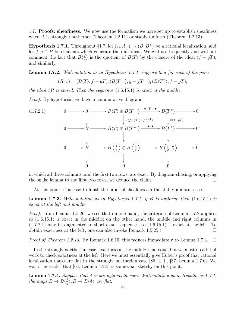
1.7. Proofs: sheafiness. We now use the formalism we have set up to establish sheafinesswhen A is strongly noetherian (Theorem 1.2.11) or stably uniform (Theorem 1.2.13).

Hypothesis 1.7.1. Throughout §1.7, let (A,A+)→ (B,B+) be a rational localization, andlet f, g ∈ B be elements which generate the unit ideal. We will use frequently and withoutcomment the fact that B〈f

g〉 is the quotient of B〈T 〉 by the closure of the ideal (f − gT ),

and similarly.

Lemma 1.7.2. With notation as in Hypothesis 1.7.1, suppose that for each of the pairs

(R, x) = (B〈T 〉, f − gT ), (B〈T−1〉, g − fT−1), (B〈T±〉, f − gT ),

the ideal xR is closed. Then the sequence (1.6.15.1) is exact at the middle.

Proof. By hypothesis, we have a commutative diagram

(1.7.2.1) 0 // 0 //

B〈T 〉 ⊕B〈T−1〉 •+T−1• //

×(f−gT,g−fT−1)

B〈T±〉 //

×(f−gT )

0

0 // B //

B〈T 〉 ⊕B〈T−1〉 •−• //

B〈T±〉 //

0

0 // B //

B⟨fg

⟩⊕B

⟨gf

⟩//

B⟨fg, gf

⟩//

0

0 0 0

in which all three columns, and the first two rows, are exact. By diagram-chasing, or applyingthe snake lemma to the first two rows, we deduce the claim.

At this point, it is easy to finish the proof of sheafiness in the stably uniform case.

Lemma 1.7.3. With notation as in Hypothesis 1.7.1, if B is uniform, then (1.6.15.1) isexact at the left and middle.

Proof. From Lemma 1.5.26, we see that on one hand, the criterion of Lemma 1.7.2 applies,so (1.6.15.1) is exact in the middle; on the other hand, the middle and right columns in(1.7.2.1) may be augmented to short exact sequences, so (1.6.15.1) is exact at the left. (Toobtain exactness at the left, one can also invoke Remark 1.5.25.)

Proof of Theorem 1.2.13. By Remark 1.6.15, this reduces immediately to Lemma 1.7.3.

In the strongly noetherian case, exactness at the middle is no issue, but we must do a bit ofwork to check exactness at the left. Here we must essentially give Huber’s proof that rationallocalization maps are flat in the strongly noetherian case [86, II.1], [87, Lemma 1.7.6]. Wewarn the reader that [64, Lemma 4.2.5] is somewhat sketchy on this point.

Lemma 1.7.4. Suppose that A is strongly noetherian. With notation as in Hypothesis 1.7.1,the maps B → B〈f

g〉, B → B〈 g

f〉 are flat.

29

Proof. By symmetry, we need only check the first claim. By Lemma 1.1.19, the map B[T ]→B〈T 〉 is flat; we thus obtain a flat map

B =B[T ]

(f − gT )→ B〈T 〉

(f − gT )= B

⟨f

g

⟩,

using Corollary 1.1.15 to make the last identification.

Lemma 1.7.5. With notation as in Hypothesis 1.7.1, if the map B → B〈fg〉 ⊕B〈 g

f〉 is flat,

then it is faithfully flat.

Proof. By [152, Tag 00HQ], it suffices to show that the image of the map

Spec

(B

⟨f

g

⟩⊕B

⟨g

f

⟩)→ Spec(B)

includes every maximal ideal m of B. To see this, note that since m is necessarily closed(see Remark 1.1.1), B/m is again a nonzero Huber ring and so has nonzero spectrum (byLemma 1.5.16); we can thus choose v ∈ Spa(B,B+) containing m in its kernel. The pointv must appear in the spectra of one of B〈f

g〉 or B〈 g

f〉; taking the kernel of the resulting

valuation gives a prime ideal of the corresponding ring which contracts to m.

Lemma 1.7.6. Suppose that A is strongly noetherian. With notation as in Hypothesis 1.7.1,(1.6.15.1) is exact at the left and middle.

Proof. By Corollary 1.1.15, every ideal of B〈T 〉 is closed; by Lemma 1.7.2, this means that(1.6.15.1) is exact at the middle. To show exactness at the left, note that the map in questionis flat by Lemma 1.7.4, and hence faithfully flat by Lemma 1.7.5.

Proof of Theorem 1.2.11. By Remark 1.6.15, this reduces immediately to Lemma 1.7.6.

1.8. Proofs: acyclicity. We next turn to acyclicity of sheaves associated to finite projectiveA-modules (Theorem 1.3.4). Throughout §1.8, continue to set notation as in Hypothesis 1.7.1.

Lemma 1.8.1. With notation as in Hypothesis 1.7.1, the map B〈fg〉 ⊕ B〈 g

f〉 → B〈f

g, gf〉 is

strict surjective, i.e., the sequence (1.6.15.1) is always strict exact at the right.

Proof. In the commutative diagram

B〈T 〉 ⊕B〈T−1〉 //

B〈T±〉

B⟨fg

⟩⊕B

⟨gf

⟩// B⟨fg, gf

⟩both vertical arrows and the top horizontal arrow are strict surjections; this yields the claim.

Proof of Theorem 1.3.4. Since M is a direct summand of a finite free A-module, we mayassume without loss of generality that M = A. By Remark 1.6.15, this reduces immediatelyto Lemma 1.8.1.

To obtain acyclicity for M for more general M , we must study the sequence (1.6.15.1) abit more closely. A key step is the following converse of sorts to Lemma 1.7.2.

30

Lemma 1.8.2. With notation as in Hypothesis 1.7.1, suppose that (1.6.15.1) is exact at theleft and middle (e.g., because A is sheafy). Then multiplication by f − gT defines injectivemaps B〈T 〉 → B〈T 〉, B〈T±〉 → B〈T±〉 with closed image.Proof. We treat the case of B〈T 〉, the case of B〈T±〉 being similar. We first argue that wemay check the claim after replacing B with each of B〈f

g〉, B〈 g

f〉, B〈f

g, gf〉. Given these cases,

for x ∈ B〈T 〉, we may recover x from x(f − gT ) by doing so in each of B〈fg, T 〉 and B〈 g

f, T 〉

and noting that the answers must agree in B〈fg, gf, T 〉. Since (1.6.15.1) is strict exact (by our

hypothesis plus Lemma 1.8.1 and Theorem 1.1.9), it follows that the map x(f − gT ) 7→ x iscontinuous, as desired.

Now promote B to a Banach ring as per Remark 1.5.4, and let GrB denote the associatedgraded ring (Definition 1.5.3), so that GrB〈T 〉 = (GrB)[T ] with T placed in degree 1.By our initial reduction, we may assume that either g = 1 and |f | ≤ 1, or f = 1 and|g| ≤ 1. (Namely, when passing from B to B〈f

g〉 or B〈 g

f〉, we replace f, g with f

g, 1 or with

1, gf.) Consequently, we may assume that the image of g − fT in GrB〈T 〉 has the form

x = x0 + x1T with 1 ∈ x0, x1. It follows easily from this (by examining the effect ofmultiplication by x on constant and leading coefficients; see also Exercise 1.8.3) that x isnot a zero-divisor in GrB〈T 〉. This in turn implies that multiplication by g− fT defines anisometric (hence strict) inclusion of B〈T 〉 into itself, thus proving the claim.

We mention a purely algebraic fact related to the proof of Lemma 1.8.2.Exercise 1.8.3. Let R be a ring. Let f ∈ R[T1, . . . , Tn] be a polynomial whose coefficientsgenerate the unit ideal in R. Prove that f is not a zero-divisor in R[T1, . . . , Tn].Remark 1.8.4. Lemma 1.8.2 provides a key special case of Theorem 1.2.7: if either of theideals (T − f) or (1− fT ) in A〈T 〉 is not closed for some f ∈ A, then A is not sheafy. Thisis precisely the mechanism of Mihara’s example [126, Proposition 3.14]; we have not checkedwhether the same criterion applies directly to the example of Buzzard–Verberkmoes.Remark 1.8.5. At this point, it is tempting to try to emulate the proof of [64, Lemma 4.2.5]to show that the sequence (1.6.15.1), if it is exact, also splits in the category of topologicalB-modules. However, this is not true in general; the proof of [64, Lemma 4.2.5] is corre-spondingly incorrect, although the result stated there does turn out to be correct for otherreasons. A related phenomenon is that for R a ring and f ∈ R, in general the exact sequence

0→ R→ R

[1

f

]⊕R

[1

1− f

]→ R

[1

f,

1

1− f

]→ 0

does not necessarily split in the category of A-modules.1.9. Proofs: vector bundles and pseudocoherent sheaves. We finally establish thelocal nature of sheafiness (Theorem 1.2.22), the base change property for pseudocoherentmodules (Theorem 1.4.13), the acyclicity of sheaves associated to pseudocoherent modules(Theorem 1.4.15), the glueing theorems for vector bundles (Theorem 1.4.2) and pseudo-coherent sheaves (Theorem 1.4.17), and corollaries (Theorem 1.4.19 and Theorem 1.4.20).Throughout §1.9, continue to set notation as in Hypothesis 1.7.1; in order to address Theo-rem 1.2.22, we refrain from globally assuming that A is sheafy.

In order to treat the two glueing theorems in parallel, we start with the base change andacyclicity arguments.

31

Remark 1.9.1. We will use in a couple of places the fact that the analogue of the sequence(1.6.15.1) with B, f, g replaced by B〈f

g〉, f

g, 1 is the sequence

0→ B

⟨f

g

⟩→ B

⟨f

g

⟩⊕B

⟨f

g,g

f

⟩→ B

⟨f

g,g

f

⟩→ 0,

which is trivially exact.

Lemma 1.9.2. With notation as in Hypothesis 1.7.1, suppose that g ∈ 1, 1− f. Then forany M ∈ PCohB, we have TorB1 (M,B〈 g

f〉) = 0.

Proof. As in Remark 1.6.17, we may use the equality B⟨

1−ff

⟩= B

⟨1f

⟩to reduce to the

case g = 1. By Lemma 1.1.18, for M ∈ PCohB, we may identify M ⊗B B〈T 〉 with M〈T 〉; inparticular, we have an exact base extension functor PCohB → PCohB〈T 〉. Now let MJT Kbe the set of formal sums

∑∞n=0 xnT

n with xn ∈ M with no convergence condition on thesequence xn; on MJT K, multiplication by 1 − fT has an inverse given by multiplicationby 1 + fT + f 2T 2 + · · · . It follows that multiplication by 1 − fT on M〈T 〉 is injective, soTorB1 (M,B〈 1

f〉) = 0 as desired.

Lemma 1.9.3. With notation as in Hypothesis 1.7.1, suppose that g ∈ 1, 1 − f and(1.6.15.1) is exact (e.g., because A is sheafy). Then we have exact base extension functors

PCohB → PCohB〈 fg〉, PCohB → PCohB〈 g

f〉, PCohB → PCohB〈 f

g, gf〉 .

Proof. Given M ∈ PCohB, choose a short exact sequence 0 → N → F → M → 0 ofB-modules with F finite free; we then have N ∈ PCohB by Remark 1.4.10. In the diagram

N〈T 〉 //

×g−fT

F 〈T 〉

×g−fT

N〈T 〉 // F 〈T 〉

we may see that the left vertical arrow is a strict inclusion by tracing around the diagram:both horizontal arrows are strict inclusions by Lemma 1.1.18, while the right vertical arrow isa strict inclusion by Theorem 1.1.9 plus Lemma 1.8.2. It follows thatM〈T 〉/(g−fT )M〈T 〉 ∼=M⊗BB〈 gf 〉 is complete for the natural topology; combining this with Lemma 1.9.2, we obtainthe exact base extension functor PCohB → PCohB〈 g

f〉.

Using Remark 1.9.1, we may repeat the argument to obtain the exact base extensionfunctor PCohB〈 g

f〉 → PCohB〈 f

g, gf〉 and the equality TorB1 (M,B〈f

g, gf〉) = 0. Using the latter,

we may tensor (1.6.15.1) with M to obtain an exact sequence

0→M →M ⊗B(B

⟨f

g

⟩⊕B

⟨g

f

⟩)→M ⊗B

⟨f

g,g

f

⟩→ 0

from which we see (using Exercise 1.4.11) that M ⊗B B〈fg〉 is complete for the natural

topology. We thus obtain the exact base extension functor PCohB → PCohB〈 fg〉.

Proof of Theorem 1.4.13. By Remark 1.6.17, this reduces immediately to Lemma 1.9.3. 32

Lemma 1.9.4. With notation as in Hypothesis 1.7.1, suppose that g ∈ 1, 1 − f and(1.6.15.1) is exact (e.g., because A is sheafy). Then for anyM ∈ PCohB, tensoring (1.6.15.1)over B with M yields another exact sequence.

Proof. Let 0 → N → F → M → 0 be an exact sequence of B-modules with F finite free;we then have N ∈ PCohA by Remark 1.4.10. By Lemma 1.9.3, tensoring this sequence overB with B〈f

g, gf〉 yields another exact sequence; it follows that TorB1 (M,B〈f

g, gf〉) = 0. This

proves the claim.

Proof of Theorem 1.4.15. By Remark 1.6.15, this reduces immediately to Lemma 1.9.4.

With Theorems 1.4.13 and 1.4.15 in hand, we now begin to work on glueing. The followinglemma is essentially [107, Lemma 2.7.2]; compare [64, Lemma 4.5.3].

Lemma 1.9.5. With notation as in Hypothesis 1.7.1, there exists a neighborhood U of 0 inB〈f

g, gf〉 such that for every positive integer n, every matrix V ∈ GLn(B〈f

g, gf〉) for which

V − 1 has entries in U can be factored as V1 · V2 with V1 ∈ GLn(B〈fg〉), V2 ∈ GLn(B〈 g

f〉).

Proof. This is a direct consequence of Lemma 1.8.1 via a contraction mapping argument.

The following lemma combines [107, Lemma 1.3.8, Lemma 2.7.4], together with some minormodifications to work around the fact that we are not limiting ourselves to simple Laurentcoverings. (The relevant special feature of a Laurent covering is that the map B〈 1

f〉 → B〈f, 1

f〉

has dense image.)

Lemma 1.9.6. With notation as in Hypothesis 1.7.1, let M1,M2,M12 be finitely generatedmodules over B〈f

g〉, B〈 g

f〉, B〈f

g, gf〉, respectively, and let ψ1 : M1 ⊗B〈 f

g〉 B〈

fg, gf〉 → M12,

ψ2 : M2 ⊗B〈 gf〉 B〈fg ,

gf〉 →M12 be isomorphisms.

(a) The map ψ : M1 ⊕M2 →M12 taking (v,w) to ψ1(v)− ψ2(w) is strict surjective.(b) For M = ker(ψ), the induced maps

M ⊗B B⟨f

g

⟩→M1, M ⊗B B

⟨g

f

⟩→M2

are strict surjective.

Proof. Let v1, . . . ,vn and w1, . . . ,wn be generating sets of M1 and M2, respectively, of thesame cardinality. We may then choose n × n matrices V and W over B〈f

g, gf〉 such that

ψ2(wj) =∑

i Vijψ1(vi) and ψ1(vj) =∑

iWijψ2(wi).Choose U as in Lemma 1.9.5. Since B〈f

g〉[f−1] is dense in B〈f

g, gf〉, we can choose a nonneg-

ative integer m and an n×n matrix W ′ over B〈 gf〉 so that V (f−mW ′−W ) has entries in U .

We may thus write 1 + V (f−mW ′ −W ) = X1X−12 with X1 ∈ GLn(B〈f

g〉), X2 ∈ GLn(B〈 g

f〉).

We now define elements xj ∈M1 ⊕M2 by the formula

xj = (xj,1,xj,2) =

(∑i

fm(X1)ijvi,∑i

(W ′X2)ijwi

)(j = 1, . . . , n).

Then

ψ1(xj,1)− ψ2(xj,2) =∑i

(fmX1 − VW ′X2)ijψ1(vi) =∑i

fm((1− VW )C2)ijψ1(vi) = 0,

33

so xj ∈M . Since C1 ∈ GLn(B〈fg, gf〉), we deduce that the map M ⊗B B〈fg 〉 →M1 induces a

strict surjection onto fmM1.The induced map M ⊗B B〈fg ,

gf〉 → M12 is strict surjective (because f is invertible in

B〈fg, gf〉), so using Lemma 1.8.1 we obtain a strict surjection M ⊗B (B〈f

g〉 ⊕ B〈 g

f〉) → M12.

Since this map factors through ψ, we obtain (a).For each v ∈M2, ψ2(v) lifts toM⊗B(B〈f

g〉⊕B〈 g

f〉) as above, so we can findw1 ∈M1,w2 ∈

M2 in the images of the base extension maps from M with ψ1(w1)− ψ2(w2) = ψ2(v). Then(w1,v + w2) ∈ M , so both w2 and v + w2 are elements of M2 in the image of the baseextension map. This proves that M ⊗B B〈 gf 〉 → M2 is strict surjective; we may reverse theroles of f and g to deduce (b).

Lemma 1.9.7. With notation as in Hypothesis 1.7.1, the image of the map Spec(B〈fg〉 ⊕

B〈 gf〉)→ Spec(B) includes all maximal ideals.

Proof. By Remark 1.1.1 and Corollary 1.5.18, every maximal ideal m of B occurs as thekernel of some valuation v. That valuation extends to one of B〈f

g〉 or B〈 g

f〉, and the kernel

of that extension is a prime ideal contracting to m.

Lemma 1.9.8. With notation as in Hypothesis 1.7.1, suppose that (1.6.15.1) is exact (e.g.,because A is sheafy).

(a) There is an exact functor

FPModB〈 fg〉×FPMod

B〈 fg ,gf〉FPModB〈 g

f〉 → FPModB

given by taking equalizers. Moreover, the composition of this functor with the baseextension functor in the opposite direction is naturally isomorphic to the identity.

(b) There is an exact, fully faithful functor

PCohB〈 fg〉×PCoh

B〈 fg ,gf〉PCohB〈 g

f〉 → PCohB

given by taking equalizers. Moreover, the composition of this functor with the baseextension functor in the opposite direction is well-defined (that is, for M ∈ PCohBin the essential image, we have M ⊗B B〈∗〉 ∈ PCohB〈∗〉) and naturally isomorphicto the identity.

Proof. Set notation as in Lemma 1.9.6. To prove (a), we must check that if M1,M2,M12 arefinite projective over their respective base rings, then M is finite projective over B and themaps

(1.9.8.1) M ⊗B B⟨f

g

⟩→M1, M ⊗B B

⟨g

f

⟩→M2

are isomorphisms. Similarly to prove (b), we must check that if M1,M2,M12 are pseudoco-herent over their respective base rings, then M is pseudocoherent over B and the maps in(1.9.8.1) are again isomorphisms.

Let us treat both cases in parallel for the moment. By Lemma 1.9.6, we can choose afinite free B-module F and a (not necessarily surjective) B-linear map F → M such thatfor F1, F2, F12 the respective base extensions of F , the induced maps

F1 →M1, F2 →M2, F12 →M12

34

are surjective. Let N1, N2, N12 be the kernels of these maps and put N = ker(N1⊕N2 → N12);by applying the snake lemma to the second and third columns in the diagram

0

0

0

0 // N //

N1 ⊕N2//

N12//

0

0 // F //

F1 ⊕ F2//

F12//

0

0 // M //

M1 ⊕M2//

M12//

0

0 0 0

we obtain the first column and its exactness (minus the dashed arrows). In particular, N =ker(F →M).

It is obvious in case (a), and a consequence of Remark 1.9.1 and Lemma 1.9.4 in case (b),that

N1 ⊗B〈 fg〉 B

⟨f

g,g

f

⟩∼= N12, N2 ⊗B〈 g

f〉 B

⟨f

g,g

f

⟩∼= N12.

Consequently, in both cases the modulesN1, N2, N12 again form an object of the fiber productcategory (using in case (b) the “two out of three” property of pseudocoherent modules, as inRemark 1.4.10); hence any general statement we can make aboutM,M1,M2,M12 also appliesto N,N1, N2, N12. This means that we may apply Lemma 1.9.6 to see that the dashed arrowsin the previous diagram are surjective. Also, in the diagram

N ⊗B B⟨fg

⟩//

F ⊗B B⟨fg

⟩//

M ⊗B B⟨fg

⟩//

0

0 // N1// F1

// M1// 0

with exact rows, we know from Lemma 1.9.6 that both outside vertical arrows are surjective.Since the middle arrow is an isomorphism, we may apply the five lemma to obtain injectivityof the right vertical arrow; this (and a similar argument with M1 replaced with M2) yieldsthe fact that the maps in (1.9.8.1) are isomorphisms.

In case (b), it remains to check that M ∈ PCohB. Since M is the kernel of a strictsurjective morphism, it is complete for the subspace topology and hence for the naturaltopology. To prove that M is pseudocoherent, it will suffice to prove that for every positiveinteger m, M admits a projective resolution in which the last m terms are finite projectivemodules. This holds for m = 1 by Lemma 1.9.6 as above; however, given the claim for anygiven m, it applies not only to M but also to N , which formally implies the claim about Mfor m+ 1. We may thus conclude by induction on m.

In case (a), it remains to check that M ∈ FPModB. To establish this, note that M isfinitely presented (by the previous paragraph) and Mm is a finite free Bm-module for every

35

maximal ideal m of B (by Lemma 1.9.7). By [152, Tag 00NX], M is a finite projectiveB-module.

Proof of Theorem 1.4.2. By Remark 1.6.16, this reduces immediately to the statement thatwith notation as in Hypothesis 1.7.1,

FPModB → FPModB〈 fg〉×FPMod

B〈 fg ,gf〉FPModB〈 g

f〉

is an exact equivalence of categories. This functor is fully faithful by Theorem 1.3.4, exacttrivially, and essentially surjective by Lemma 1.9.8(a).

Proof of Theorem 1.4.17. By Remark 1.6.16, this reduces immediately to the statement thatwith notation as in Hypothesis 1.7.1 with g ∈ 1, 1 − f, there is an exact equivalence ofcategories

(1.9.8.2) PCohB → PCohB〈 fg〉×PCoh

B〈 fg ,gf〉PCohB〈 g

f〉

To begin with, by Lemma 1.9.3 we obtain exact base extension functors from PCohB toeach of PCohB〈 f

g〉, PCohB〈 g

f〉, PCohB〈 f

g, gf〉. This yields an exact functor as in (1.9.8.2); this

functor is fully faithful by Lemma 1.9.4 and essentially surjective by Lemma 1.9.8(b).

Remark 1.9.9. One source of inspiration for the preceding arguments is the Beauville–Laszlo theorem [11], [152, Tag 0BNI], [14], which asserts (among other things) that if R is aring, f ∈ R is not a zero-divisor, and R is the f -adic completion of R, then the functor

FPModR → FPModRf×FPMod

RfFPModR

is an equivalence of categories. See [107, Remark 2.7.9] for further explanation of how thisresult can be derived in the style of the arguments given above.

Another similarity that should be noted is that the Beauville–Laszlo theorem was origi-nally introduced in order to construct and study affine Grassmannians associated to algebraicgroups in the context of geometric Langlands. The glueing results discussed here are them-selves relevant for the construction and study of certain mixed-characteristic analogues ofaffine Grassmannians, to be introduced in a later lecture (§4.6).

Proof of Theorem 1.4.19. Choose parameters f1, . . . , fm, g defining the rational localization(A,A+) → (B,B+). By Theorem 1.4.17, we may prove the claim locally on X; using thestandard rational covering defined by f1, . . . , fm, g, we reduce to the situation where oneof f1, . . . , fm, g is itself a unit. In this case (A,A+) → (B,B+) factors as a composition ofrational localizations, each of which occurs in a simple Laurent covering:

• if g is a unit, then the rational subspace is defined by the conditions v(f1/g) ≤1, . . . , v(fn/g) ≤ 1;• if f1 is a unit, then after imposing the condition v(g/f1) ≥ 1, g becomes a unit andwe may continue as in the previous case.

We are thus reduced to checking the claim in case B is the quotient of A〈U〉 by the closureof the ideal generated by either f −U or 1−fU for some f ∈ A. In these cases, we have B ∈PCohA〈U〉 by Lemma 1.8.2: in fact, B is not only pseudocoherent but of projective dimension≤ 1 as an A〈U〉-module. For any surjective homomorphism g : A〈T1, . . . , Tn〉 → B, chooselifts y1, . . . , yn of g(T1), . . . , g(Tn) to A〈U〉. Via the morphism A〈T1, . . . , Tn, U〉 → A〈U〉taking Ti to yi, we have A〈U〉 ∈ PCohA〈T1,...,Tn,U〉 and hence B ∈ PCohA〈T1,...,Tn,U〉. Now

36

choose a lift z to A〈T1, . . . , Tn〉 of the image of U in B; we may then view A〈T1, . . . , Tn〉 as aquotient of A〈T1, . . . , Tn, U〉 via the map U 7→ z, and then conclude that B ∈ PCohA〈T1,...,Tn〉.

Proof of Theorem 1.2.22. There is no harm in refining the covering V; by Lemma 1.6.12, wemay reduce to the case where V is the simple binary rational covering generated by somef, g ∈ A. By hypothesis, the sequence

0→ A→ A

⟨f

g

⟩⊕ A

⟨g

f

⟩→ A

⟨f

g,g

f

⟩→ 0

is strict exact, as then is

0→ A〈T 〉 → A

⟨f

g, T

⟩⊕ A

⟨g

f, T

⟩→ A

⟨f

g,g

f, T

⟩→ 0.

Using Lemma 1.8.2, we obtain a commutative diagram

0

0

0

0 // A〈T 〉 //

A⟨fg, T⟩⊕ A

⟨gf, T⟩

//

×g−fT

A⟨fg, gf, T⟩

//

×g−fT

0

0 // A〈T 〉 //

A⟨fg, T⟩⊕ A

⟨gf, T⟩

//

A⟨fg, gf, T⟩

//

0

0 // A⟨fg

⟩//

A⟨fg

⟩⊕ A

⟨fg, gf

⟩//

A⟨fg, gf

⟩//

0

0 0 0

in which the first and second rows are exact, the second and third columns are exact, and theleft column is exact at the top and bottom (but not a priori in the middle). By diagram chas-ing, the third row is exact. From this (and the analogous argument with f, g interchanged),we obtain natural isomorphisms

A

⟨f

g

⟩∼= A

⟨f

g

⟩, A

⟨g

f

⟩∼= A

⟨g

f

⟩, A

⟨f

g,g

f

⟩∼= A

⟨f

g,g

f

⟩;

from this we deduce (a). Note that we cannot say that any rational subspace of Spa(A, A+)arises by pullback from Spa(A,A+), since such a subspace is defined by parameters in Awhich we cannot immediately replace with parameters in A.

In light of the previous arguments, to finish the proof of both (a) and (b), it now sufficesto check (b) in the case where A = A. To this end, let (A,A+) → (B,B+) be the rationallocalization defined by the parameters h1, . . . , hn, k ∈ A, and identify B with the quotientof A〈T1, . . . , Tn〉 by the closure of the ideal generated by kT1 − h1, . . . , kTn − hn. Since wehave now established Theorem 1.4.19, it is legitimate to apply Theorem 1.2.7; hence for each

37

nonempty subset ∗ of fg, gf, we obtain an exact sequence of pseudocoherent A〈∗, T1, . . . , Tn〉-

modules of the form

(1.9.9.1) A〈∗, T1, . . . , Tn〉n → A〈∗, T1, . . . , Tn〉 → B〈∗〉 → 0

in which the first map takes the generators to kT1 − h1, . . . , kTn − hn.Although we do not know2 that A〈T1, . . . , Tn〉 is sheafy, we do have the exact sequence

0→ A〈T1, . . . , Tn〉 → A

⟨f

g, T1, . . . , Tn

⟩⊕A

⟨g

f, T1, . . . , Tn

⟩→ A

⟨f

g,g

f, T1, . . . , Tn

⟩→ 0,

using which we may apply Lemma 1.9.8 to the various objects in (1.9.9.1). This yields anotherexact sequence

0→ (kT1 − h1, . . . , kTn − hn)→ A〈T1, . . . , Tn〉 → H0(Spa(B,B+),O)→ 0

of pseudocoherent A〈T1, . . . , Tn〉-modules. In particular, the ideal (kT1 − h1, . . . , kTn − hn)is closed; it follows that B = H0(Spa(B,B+),O), as desired.

Lemma 1.9.10. Let I be a (not necessarily closed) ideal of A. For any f1, . . . , fn ∈ A whichgenerate the unit ideal in A/I, there exists a rational localization (A,A+) → (B,B+) suchthat Spa(B,B+) contains the zero locus of I on Spa(A,A+) and f1, . . . , fn generate the unitideal in B.

Proof. By hypothesis, there exist b1, . . . , bn ∈ A such that a1b1 + · · ·+anbn ≡ 1 (mod I). Therational localization corresponding to the subspace v ∈ Spa(A,A+) : v(a1b1 + · · ·+ anbn) ≥1 has the desired property.

Lemma 1.9.11. Let I be a closed ideal of A which is an object of PCohA. Let (A,A+) →(B,B+) be a rational localization.

(a) Put A := A/I and let A+ be the integral closure of the image of A+ in A. Let(A,A

+) → (B,B

+) be the base extension of the given rational localization. Then

B ∼= B/IB.(b) Suppose that Spa(B,B+) contains the zero locus of I on Spa(A,A+). Then A/IA ∼=

B/IB.

Proof. By Theorem 1.4.13, the sequence

0→ I → A→ A/I → 0

remains exact upon tensoring over A with B. In particular, IB ∼= I⊗B ∈ PCohB is a closedideal, so B/IB coincides with the completed tensor product B⊗AA/I; this proves (a). From(a), (b) is obvious.

Proof of Theorem 1.4.20. Put A := A/I and let A+ be the integral closure of the image ofA+ in A. By Remark 1.6.15, it suffices to check that for any rational localization (A,A

+)→

(B,B+

) and any f, g ∈ B with g ∈ 1, 1− f, the sequence

0→ B → B

⟨f

g

⟩⊕B

⟨g

f

⟩→ B

⟨f

g,g

f

⟩→ 0

2In fact, even knowing that A is sheafy would not imply that A〈T1, . . . , Tn〉 is sheafy!38

is exact. By Lemma 1.9.11, there is no harm in replacing (A,A+) with the rational localizationcorresponding to a subspace containing the zero locus of I on Spa(A,A+). By Lemma 1.9.10,we may thus ensure that some set of parameters in A defining the rational localization(A,A

+) → (B,B

+) lift to elements of A which generate the unit ideal. By Lemma 1.9.11

again, there is no harm in replacing (A,A+) by the corresponding rational localization; thatis, we may assume that (A,A

+) = (B,B

+).

Lift f, g to f, g ∈ A with g ∈ 1, 1− f. In the diagram

0

0

0

0 // IA //

IA⟨fg

⟩⊕ IA

⟨gf

⟩//

IA⟨fg, gf

⟩//

0

0 // A //

A⟨fg

⟩⊕ A

⟨gf

⟩//

A⟨fg, gf

⟩//

0

0 // A //

A⟨fg

⟩⊕ A

⟨g

f

⟩//

A⟨fg, gf

⟩//

0

0 0 0

the second row is exact by the sheafiness of A, the first row is exact by Theorem 1.4.13,the first column is exact by definition, and the second and third columns are exact byLemma 1.9.11. This implies exactness of the third row, as needed.

1.10. Remarks on the etale topology. As promised at the end of §1.4, we include someremarks about the etale topology on X.

Lemma 1.10.1. Suppose that A is uniform. Then every finite etale A-algebra is uniformfor its natural topology as an A-module.

Proof. In the case where A is Tate, this is [107, Proposition 2.8.16]. The analytic case canbe treated similarly, but can also be handled as follows. Extend A to a Huber pair (A,A+),let B be a finite etale A-algebra of constant rank (it suffices to treat this case), and let B+

be the integral closure of A+ in B. Since B is finitely generated as an A-module and theunit ideal of A is generated by topologically nilpotent elements, we can find b1, . . . , bn ∈ B+

which generate B as an A-module. We now see B+ is contained in the set

b ∈ B : TraceB/A(bb1), . . . ,TraceB/A(bbn) ∈ A+,which is bounded (because the trace pairing is nondegenerate); hence B is uniform.

Remark 1.10.2. Let B be a finite etale A-algebra and let B+ be the integral closure of A+ inB. If A is strongly noetherian, then so is B, so there are no technical issues with consideringthe etale site of X. On the other hand, if A is only sheafy, or even stably uniform, thenwe cannot immediately infer the same about B: we have the sheaf axiom for coverings ofSpa(B,B+) arising by pullback from X, but any covering that separates points within some

39

fiber of the projection Spa(B,B+)→ X will fail to be refined by such a covering. (That said,we do not have a counterexample in mind.)

In light of the previous remark, we make the following hypothesis.

Hypothesis 1.10.3. For the remainder of §1.10, let Xet be the site whose morphisms arecompositions of rational localizations and finite etale morphisms. (Note that this gives the“right” definition of the etale site for analytic adic spaces, but not for schemes.) Assume thatXet admits a basis B closed under formation of rational localizations and finite etale covers,and consisting of subspaces of the form Spa(B,B+) where B is sheafy. For example, thishypothesis is satisfied if A is perfectoid, or even sousperfectoid (see Remark 1.2.19).

For the etale topology, one has the following analogue of Lemma 1.6.18; however, the proofis somewhat less straightforward, and uses a method introduced by de Jong–van der Put [34,Proposition 3.2.2].

Lemma 1.10.4. Let Pet be the collection3 of pairs (U,V) where U ∈ B and V is a finitecovering of U in Xet by elements of B. Suppose that P ⊆ Pet satisfies the following conditions.

(i) Locality: if (U,V) admits a refinement in P, then (U,V) ∈ P.(ii) Transitivity: Any composition of coverings in P is in P.(iii) Every standard binary rational covering is in P.(iv) Every finite etale surjective morphism, viewed as a covering, is in P.

Then P = Pet.

Proof. See [107, Proposition 8.2.20].

Remark 1.10.5. Using Lemma 1.10.4, it is straightforward to extend Theorems 1.3.4, 1.4.2,1.4.13, 1.4.15, and 1.4.17 to Xet; we leave the details to the reader.

1.11. Preadic spaces. We end with a remark about how to formally build “spaces” out ofHuber pairs even when they are not sheafy. This discussion is taken from [148, §2], althoughour terminology4 instead follows [107, §8.2]. (To keep within our global context, we buildonly analytic preadic spaces here.)

Definition 1.11.1. For C a category equipped with a Grothendieck topology (so in particularadmitting fiber products), a sheaf on C is by definition a contravariant functor F from C tosome target category satisfying the sheaf axiom: for Ui → Xi a covering in C, the sequence

F (X)→∏i

F (Ui)⇒∏i,j

F (Ui ×X Uj)

is an equalizer.We say that C is subcanonical if for each X ∈ C, the representable functor hX : Y 7→

HomC(Y,X) is a sheaf. For example, the Zariski topology on schemes is subcanonical: thisreduces immediately to the corresponding statement for affine schemes, which asserts thatif R and S are rings and f1, . . . , fn ∈ R generate the unit ideal in R, then the diagram

Hom(S,R)→∏i

Hom(S,Rfi)⇒∏i,j

Hom(S,Rfifj)

3This is not a set in general, but a proper class.4In [148], what we call preadic spaces and adic spaces are called adic spaces and honest adic spaces,

respectively. We prefer to leave the term adic spaces with the original meaning specified by Huber.40

is an equalizer; this follows from the sheaf axiom for the structure sheaf. By the samereasoning, the etale, fppf, and fpqc topologies on the category of schemes are subcanonical.

Similarly, if C is a subcategory of the category of adic spaces admitting fiber products(e.g., locally noetherian spaces, or perfectoid spaces), the analytic topology on C (i.e., thesite coming from the underlying topology on underlying spaces) is subcanonical. By contrast,the analytic topology on the full category of Huber pairs is not subcanonical.

Definition 1.11.2. Let C be the opposite category of (analytic but not necessarily sheafy)Huber pairs, equipped with the analytic topology. Let C∼ be the associated topos. For(A,A+) ∈ C, let Spa(A,A+) ∈ C∼ be the sheafification of the representable functor on Cdefined by (A,A+).

By an open immersion in C∼, we will mean a morphism f : F → G such that for every(A,A+) ∈ C and every morphism Spa(A,A+) → G in C∼, there is an open subset U ofSpa(A,A+) such that

F ×G Spa(A,A+) = lim−→V⊆U,V rational

Spa(OSpa(A,A+)(V ),O+Spa(A,A+)(V )).

A preadic5 space, or more precisely an analytic preadic space, is an object F ∈ C∼ such that

F = lim−→Spa(A,A+)→F open

Spa(A,A+).

The obvious functor from analytic adic spaces to analytic preadic spaces is a full embedding.A morphism f : F → G is finite etale if for every (A,A+) ∈ C and every morphism

Spa(A,A+) → G in C∼, we have F ×G Spa(A,A+) ∼= Spa(B,B+) for some finite etalemorphism (A,A+) → (B,B+). Using finite etale morphisms and open immersions, we maydefine the etale topology on analytic preadic spaces.

Remark 1.11.3. Similar sheaf-theoretic considerations give rise to other types of objectsthat one might think of as analytic analogues of algebraic spaces (or more generally algebraicstacks). Notably, they underlie the construction of diamonds, which will be introduced in[163, Lecture 3] and used in our subsequent lectures (see Definition 4.3.1 and beyond).

5Or pre-adic space if you prefer to hyphenate prefixes.41

2. Perfectoid rings and spaces

In this lecture, we define perfectoid rings and spaces, picking up from the discussionof perfectoid fields in [163, Lecture 2]. As for fields, there is a “tilting” construction thatconverts these spaces into related objects in characteristic p; however, this time the “Galois”component of the tilting correspondence is augmented by a “spatial” component.

As in the first lecture, we state all of the main results first, then return to the proofs.Along the way, we attempt to lay flat some of the tangled history6 surrounding these results.

Hereafter, we fix a prime number p and consider only Huber rings in which p is topologicallynilpotent.

2.1. Perfectoid rings and pairs. We now define perfectoid rings and pairs, postponingsome proofs for the time being.

Definition 2.1.1. Let (A,A+) be a uniform analytic Huber pair; by uniformity, A+ is a ringof definition of A. We say (A,A+) is perfectoid if there exists an ideal of definition I ⊆ A+

such that p ∈ Ip and ϕ : A+/I → A+/Ip is surjective (but not necessarily injective; seeRemark 2.3.16). This turns out to depend only on A (Corollary 2.3.10); we may thus sayalso that A is a perfectoid ring.

Example 2.1.2. If (A,A+) is a uniform analytic Huber pair of characteristic p, then (A,A+)is perfectoid if and only if A is perfect: if A is perfect, then A+ must also be perfect becauseit is integrally closed in A.

Example 2.1.3. Any algebraically closed nonarchimedean field is a perfectoid ring. Moregenerally, recall that a perfectoid field is defined as a nonarchimedean field F which is notdiscretely valued for which ϕ : oF/(p) → oF/(p) is surjective. If F is a perfectoid field,then (F, oF ) is a perfectoid Huber pair; this is obvious in characteristic p (because F is thenperfect), and otherwise we may take I = (µ) for any topologically nilpotent element µ suchthat µp divides p in oF (which exists because F is not discretely valued). Conversely, if Ais a perfectoid ring which is a field, then A is a perfectoid field; see Corollary 2.3.11 andTheorem 2.9.1.

Example 2.1.4. Let (A,A+) be any perfectoid Huber pair (e.g., (F, oF ) for F a perfectoidfield as in Example 2.1.3). Then for every nonnegative integer n,

(A〈T p−∞

1 , . . . , T p−∞

n 〉, A+〈T p−∞

1 , . . . , T p−∞

n 〉)and

(A〈T±p−∞

1 , . . . , T±p−∞

n 〉, A+〈T±p−∞

1 , . . . , T±p−∞

n 〉)are also perfectoid Huber pairs.

Remark 2.1.5. If (A,A+) is perfectoid, then ϕ : A+/((p) + I)→ A+/((p) + Ip) is surjectivefor any ideal of definition I as in Definition 2.1.1. By Lemma 2.7.4, the same is true for anyideal of definition I whatsoever. In particular, the criterion of Definition 2.1.1 is satisfiedfor every ideal of definition I for which p ∈ Ip. However, the existence of such an ideal

6I am reminded here of a famous quote of David Mumford [128, Preface]: “When I first started doingresearch in algebraic geometry, I thought the subject attractive... because it was a small, quiet field where adozen people did not leap on each new idea the minute it became current.”

42

of definition is a genuine condition; for instance, it precludes the case (Qp,Zp), for whichϕ : A+/((p) + I)→ A+/((p) + Ip) is surjective for any ideal of definition I.

Note that the previous paragraph does not immediately imply that ϕ : A+/(p)→ A+/(p)is surjective. However, this will follow from the tilting correspondence (Theorem 2.3.9); seeRemark 2.3.12.

Remark 2.1.6. Note that for A a perfectoid ring, the ring A〈T p−∞

1 , . . . , T p−∞

n 〉 of Exam-ple 2.1.4 is evidently not noetherian: the ideal (T p

−n

1 : n = 0, 1, . . . ) is not finitely generated.In fact, perfectoid rings can never be noetherian except in the trivial case where they arefinite direct sums of perfectoid fields; see Corollary 2.9.3.

This means that we cannot hope to use noetherian properties to show that perfectoidrings are sheafy. Instead, we will have to show that they are stably uniform, by establishingthe preservation of the perfectoid property under rational localizations using the tiltingconstruction (Corollary 2.5.4).

Remark 2.1.7. For (A,A+) a perfectoid ring, I an ideal of definition as in Definition 2.1.1,and (A,A+) → (B,B+) a morphism of uniform Huber pairs, the pair (B,B+) is perfectoidif and only if ϕ : B+/IB+ → B+/IpB+ is surjective. This is a consequence of Remark 2.1.5,which allows us to use IB+ as an ideal of definition to check the perfectoid condition.

We record some historical aspects of the definition of perfectoid fields and rings.

Remark 2.1.8. The term perfectoid was introduced by Scholze [142], but various aspectsof the general concept had appeared several times before then. Here we report on theseappearances.

The term perfectoid field was introduced by Scholze in [142]. A similar definition wasgiven independently7 by Kedlaya in [101] and incorporated into the work of Kedlaya–Liu[107]; while much of the work on [107] predates the appearance of [142], some terminologyfrom the latter was adapted in the published version of the former. See Remark 2.5.12 formore details. It was subsequently discovered that Matignon–Reversat [125] had introducedthe same concept in 1984 as a hyperperfect field (corps hyperparfait), but the importance ofthis development seems to have gone unnoticed at the time.

Some examples of perfectoid rings which are not fields appear in the hypothesis of thealmost purity theorem of Faltings [51, Theorem 3.1], [53, Theorem 4]. These examples servedas a key motivation for the general construction.

In [27], Colmez introduces the concept of a sympathetic algebra (algebre sympathique),which is equivalent to a perfectoid ring over an algebraically closed perfectoid field. He thenuses these rings to define what are commonly known as Banach-Colmez spaces, which willbe discussed in [163, Lecture 4] and used in our student project.

The term perfectoid ring was introduced in [142] to refer to a perfectoid ring in thepresent sense over an arbitrary perfectoid field. The concept of a perfectoid ring over Qp

was introduced independently by Kedlaya–Liu [107], with terminology adapted from [142];this excludes perfectoid rings of characteristic p, which appear separately in [107] as perfectuniform Banach Fp-algebras. Some alternate characterizations of perfectoid rings over Qp,phrased in terms of Witt vectors, can be found in [30].

7The paper [101] was originally written as a supplement to the lecture notes from the 2009 Clay Mathe-matics Institute summer school on p-adic Hodge theory. As of this writing, those notes remain unpublished.

43

In his Bourbaki seminar on the work of Scholze, Fontaine [61] introduced the concept ofa Tate perfectoid ring, phrasing the definition in terms of condition (a) of Corollary 2.6.16.As [61] is primarily a survey of [142], the theory of Tate perfectoid rings is not developed inany detail there; this development was subsequently carried out by Kedlaya–Liu [108]. Notethat in characteristic p, a perfectoid ring is Tate precisely when it admits the structure ofan algebra over some perfectoid field.

The definition of perfectoid rings used here, which allows for arbitrary analytic rings, isoriginal to these notes. For examples that separate the various definitions, see the followingreferences herein:

• for a perfectoid ring over Qp which is not an algebra over a perfectoid field, seeExercise 2.4.10;• for a perfectoid ring which is Tate but not a Qp-algebra, see the proof of Lemma 3.1.3;• for a perfectoid ring which is analytic but not Tate, see Exercise 2.4.11.

The massive work-in-progress [65] should ultimately be even more inclusive, in ways we donot attempt to treat here (for instance, it includes some rings which are not analytic).

2.2. Witt vectors. In order to say more about perfectoid rings, we need to recall somebasic facts about Witt vectors (compare [101, §1.1]).

Definition 2.2.1. A ring of characteristic p is perfect if the absolute Frobenius map is abijection. A strict p-ring is a p-adically complete (so in particular p-adically separated) ringS which is flat over Zp (that is, p is not a zero-divisor) with the property that S/pS is perfect.

Example 2.2.2. The ring S := Zp is a strict p-ring with S/pS ∼= Fp. Similarly, for any finiteunramified extension F of Qp with residue field Fq, the integral closure S of Zp in F is astrict p-ring with S/pS ∼= Fq. Similarly, for F the maximal unramified extension of Qp, thecompleted integral closure S of Zp in F is a strict p-ring with S/pS ∼= Fp.

Example 2.2.3. For n a nonnegative integer, the p-adic completion S of Z[T p−∞

1 , . . . , T p−∞

n ]

is a strict p-ring with S/pS ∼= Fp[Tp−∞

1 , . . . , Tp−∞

n ].

Lemma 2.2.4. For any ring R, any ideal I of R, and any nonnegative integer n, the mapx 7→ xp

n induces a morphism of multiplicative monoids

R/((p) + I)→ R/((p)n+1 + (p)nI + · · ·+ (p)Ipn−1

+ Ipn

).

Proof. This is an immediate consequence of the p-divisibility of binomial coefficients.

Corollary 2.2.5. For S a strict p-ring, the map S → S/pS admits a unique multiplicativesection x 7→ [x], called the Teichmuller map. In particular, the element [x] ∈ S (called theTeichmuller lift of x) is the unique lift of x which admits pn-th roots for all positive integersn.

Corollary 2.2.6. For S a strict p-ring, every element x of S has a unique representation asa p-adically convergent series

∑∞n=0 p

n[xn] with xn ∈ S/pS. The xn are called the Teichmullercoordinates of x.

Lemma 2.2.7. Let S be a strict p-ring. Let S ′ be any p-adically complete ring. Then everyring homomorphism π : S/pS → S ′/pS ′ lifts uniquely to a homomorphism S → S ′.

44

Proof. By Lemma 2.2.4, π lifts uniquely to a multiplicative map π : S/pS → S ′. One thenshows that the formula

∞∑n=0

pn[xn] 7→∞∑n=0

pnπ(xn)

defines the desired ring homomorphism, by checking additivity modulo pm by induction onm. For details, see [101, Lemma 1.1.6].

Remark 2.2.8. By applying Lemma 2.2.7 in the case where S is as in Example 2.2.3, wemay see that arithmetic in a strict p-ring can be expressed in terms of certain universal“polynomials” in the Teichmuller coordinates. For example, if one writes

[x] + [y] =∞∑n=0

pn[zn],

then zn is given by a certain homogeneous polynomial over Fp in xp−n, yp

−n of degree 1 (forthe convention that deg(x) = deg(y) = 1) divisible by xp−n

yp−n .

Remark 2.2.9. A corollary of the previous remark is that if S is a strict p-ring and I is aperfect ideal of S/pS, then the set of x ∈ S whose Teichmuller coordinates all belong to I isan ideal of S. Note that the quotient by this ideal is again a strict p-ring.

Theorem 2.2.10 (Witt). The functor S 7→ S/pS defines an equivalence of categories be-tween strict p-rings and perfect Fp-algebras.

Proof. Full faithfulness follows from Lemma 2.2.7. To check essential surjectivity, we firstlift perfect polynomial rings over Fp in any (possibly infinite) number of variables as inExample 2.2.3, then use Remark 2.2.9 to lift quotients of such rings. That covers all perfectFp-algebras.

Remark 2.2.11. There is no analogue of Theorem 2.2.10 for general R. For example, if R isa field which is not perfect, then the Cohen structure theorem implies that R can be realizedas S/pS for some flat p-adically complete Zp-algebra S (any such S is called a Cohen ring forR), but not functorially in R. For example, if R = Fp((T )), then the p-adic completion S ofZp((T )) admits an isomorphism S/pS ∼= R taking the class of T to T , but there are numerousautomorphisms of S lifting the identity map on R; in fact, the group of such automorphismsacts simply transitively on the inverse image of T .

One way to lift imperfect rings is to consider pairs (R,B) in which R is a reduced ringof characteristic p and B is a finite subset of R such that

∏b∈B b

eb : eb ∈ 0, . . . , p − 1is a basis for Rp as an R-module. (Such a set B is called a p-basis of R; the existence ofsuch a set implies that Rp is a finite projective R-module, which is to say that R is F-split.)Then one can functorially lift (R,B) to a pair (S, B) in which S is a p-adically complete flatZp-algebra and B is a finite subset of S lifting B.

Definition 2.2.12. For R a perfect ring of characteristic p, let W (R) denote the strict p-ring with residue ring R; concretely, W (R) consists of sequences (x0, x1, . . . ) in R which areidentified with the convergent sums

∑∞n=0 p

n[xn]. By functoriality (i.e., by Lemma 2.2.7), theabsolute Frobenius ϕ on R lifts to a unique automorphism of R. For I ⊆ R a perfect ideal,let W (I) denote the ideal of W (R) described in Remark 2.2.9.

45

Remark 2.2.13. For conceptual purposes, it is sometimes useful to imagine the ring W (R)as “the ring of power series in the variable p with coefficients in R.” This point of view mustof course be abandoned when one attempts to make any arguments involving calculationsin W (R); however, Remark 2.2.8 gives some control over the “carries” that occur in thesecalculations.

2.3. Tilting and untilting. In order to say more about perfectoid rings, we describe afundamental construction that relates perfectoid rings to rings in characteristic p. This con-struction has its roots in the foundations of p-adic Hodge theory (see Remark 2.3.18), andthe definition of perfectoid rings is in turn motivated by the construction.

Definition 2.3.1. For (A,A+) a perfectoid pair, define the tilt of A, denoted A[, as the setlim←−x 7→xp A; it carries the structure of a monoid under multiplication. We equip A[ with theinverse limit topology (i.e., the coarsest topology with respect to which the map ] : A[ → Awhich projects onto the final component is continuous); this gives A[ the structure of atopological monoid. (We sometimes write x] instead of ](x).) Let A[+ be the submonoidlim←−x 7→xp A

+ of A[.We will see later (Theorem 2.3.9) that the formula

(2.3.1.1) (xn)n + (yn)n = (zn)n, zn := limm→∞

(xm+n + ym+n)pm

defines a ring structure on A[ with respect to which it is a perfectoid ring of characteristicp, in such a way that A[+ is a ring of integral elements. Another interpretation of the ringstructure on A[+ will come from the bijection

(2.3.1.2) A[+ ∼= lim←−x 7→xp

(A+/I)

for any ideal of definition I as in Definition 2.1.1; note that the right-hand side of (2.3.1.2)is obviously a perfect ring of characteristic p.

In order to fill in the details of the previous construction, we describe an inverse construc-tion using Witt vectors.

Definition 2.3.2. Let (R,R+) be a perfectoid pair in characteristic p. We will make frequentuse of the ring W (R+), which is commonly denoted Ainf(R,R

+) (although we will not usethis notation until the next lecture).

Let W b(R) denote the subset of W (R) consisting of series∑∞

n=0 pn[xn] for which the set

xn : n = 0, 1, . . . is bounded in R. By Remark 2.2.8, this forms a subring ofW (R) contain-ing W (R+). We equip W b(R) with the topology of uniform convergence in the coordinates(see Remark 2.6.3); any continuous map R→ S of perfectoid rings in characteristic p inducesa homomorphism W b(R)→ W b(S).

Remark 2.3.3. If R is Tate, then so is W b(R): for any pseudouniformizer $ in R, [$] is apseudouniformizer inW b(R). However, if R is analytic, it is not clear thatW b(R) is analytic;compare Lemma 2.6.13.

The following construction provides something analogous to a Weierstrass-prepared powerseries over a nonarchimedean field.

46

Definition 2.3.4. An element z =∑∞

n=0 pn[zn] ∈ W (R+) is primitive of degree 1 (or prim-

itive for short) if z0 is topologically nilpotent and z1 is a unit in R+; in other words,z = [z0] + pz1 where z1 is a unit in W (R+). Note that multiplying a primitive elementby a unit gives another such element (e.g., using Remark 2.2.8); we say that an ideal ofW (R+) is primitive (of degree 1) if it is principal with some (hence any) generator being aprimitive element.

The primitive elements will play a role analogous to that played by the ideal (T − p) inthe isomorphism ZJT K/(T − p) ∼= Zp. In particular, they admit a form of Euclidean divisionwhich is quite useful for getting control of elements of perfectoid rings; this will be studiedextensively in §2.6.

Remark 2.3.5. If z1, z2 ∈ W (R+) are primitive elements such that z1 = yz2 for somey ∈ W (R+), then by Remark 2.2.8, z1,1 − y0z2,1 is topologically nilpotent. It follows that yis a unit in W (R+).

Exercise 2.3.6. If R is Tate, then in some sources a primitive element ofW (R+) is assumedto have the form p+ [$]α where $ ∈ R is a topologically nilpotent unit and α ∈ W (R+) isarbitrary. Show that if z is a primitive element in the sense of Definition 2.3.4, then it hassome associate of the form p+ [$]α but need not have this form itself.

Before stating a general theorem, let us discuss a couple of key examples.

Example 2.3.7. Put R := Fp((Tp−∞

)) (i.e., the ring obtained by taking the T -adic comple-tion of Fp[T

p−∞

] and then inverting T ) and R+ := R. The element z := p− [T ] is primitive,and W b(R)/(z) is the completion of Qp(p

p−∞), which is a perfectoid field.

Example 2.3.8. Put R := Fp((Tp−∞

)), R+ := R. The element z :=∑p−1

i=0 [1 + T ]i isprimitive (because it maps to p under W (R+)→ W (Fp)), and W b(R)/(z) is the completionof Qp(µp∞), which is a perfectoid field.

Theorem 2.3.9. The formula

(2.3.9.1) (R,R+, I) 7→ (A := W b(R)/IW b(R), A+ := W (R+)/I)

defines a equivalence of categories from triples (R,R+, I), in which (R,R+) is a perfectoidpair of characteristic p and I is a primitive ideal of W (R+), to perfectoid pairs (A,A+).(A morphism (R,R+, I) → (S, S+, J) in this category is a morphism (R,R+) → (S, S+)of Huber pairs carrying I into J ; in fact, by Remark 2.3.5 the image always equals J .)Furthermore, there is a quasi-inverse functor which takes (A,A+) to (A[, A[+, I) with thering structure on A[ given by (2.3.1.1).

Proof. By Lemma 2.6.14, it will follow that the equation (2.3.9.1) gives a well-defined functor.By Lemma 2.7.9, we will obtain the quasi-inverse functor.

Corollary 2.3.10. Let A be a perfectoid ring, that is, A is a Huber ring such that (A,A+)is a perfectoid pair for some ring of integral elements A+. Then (A,A+) is a perfectoid pairfor every ring of integral elements A+.

Proof. By Theorem 2.3.9, we can write A = W b(R)/I for some perfectoid ring R of char-acteristic p and some ideal I; more precisely, the ideal I admits a primitive generator inW (R+) for some ring of integral elements R+ of R, and hence in W (R). By Example 2.1.2,

47

every ring of integral elements R+ of R untilts to a ring of integral elements A+ of A suchthat (A,A+) is perfectoid. It thus suffices to check that every A+ arises in this fashion.

Since A is uniform, every ring of integral elements is contained in the ring A of power-bounded elements and contains the set A of topologically nilpotent elements, which is anideal of A. In fact, the rings of integral elements are in bijection with integrally closed sub-rings of A/A. Similarly, the rings of integral elements of R are in bijection with integrallyclosed subrings of A/A. By Lemma 2.7.10, the rings A/A and R/R are isomorphic;this completes the proof. (See Remark 2.3.16 for a more refined version of the isomorphismA/A ∼= R/R).

Corollary 2.3.11. A nonarchimedean field F is a perfectoid ring if and only if it is aperfectoid field.

Proof. One direction is Example 2.1.3. In the other direction, if F is a perfectoid ring, thenby Corollary 2.3.10, (F, oF ) is a perfectoid pair. If F is of characteristic p, then F is perfect(Example 2.1.2) and the valuation on F is nontrivial (hence not discrete by perfectness), soF is a perfectoid field. If F is of characteristic 0, then (p) is an ideal of definition of oF , soRemark 2.3.12 applies to show that ϕ : oF/(p) → oF/(p) is surjective. Since the valuationon F [ is not discrete, neither is the valuation on F , so F is a perfectoid field.

Remark 2.3.12. If (A,A+) is a perfectoid pair, then the existence of a surjective morphismW (R+) → A+ as in Theorem 2.3.9 implies that ϕ : A+/(p) → A+/(p) is surjective: everyx ∈ A+/(p) lifts to some element y =

∑∞n=0 p

n[yn] ∈ W (R+), and the image of [y1/p0 ] in

A+/(p) maps to x via ϕ.

Definition 2.3.13. With notation as in Theorem 2.3.9, the perfectoid pair (A,A+) corre-sponding to the triple (R,R+, I) is called the untilt of (R,R+) corresponding to the primitiveideal I.

Definition 2.3.14. Theorem 2.3.9 implies that for any perfectoid pair (A,A+), there is asurjective map W (A[+)→ A+ whose kernel is primitive (and in particular principal), whichextends to a map W b(A[)→ A. These maps are traditionally denoted by θ.

Note that for any x ∈ R, the sequence (θ([xp−n

])n forms an element of lim←−x 7→xp A = A[. Inthe course of proving Theorem 2.3.9, we will see that the identification of A[ with R identifiesthis sequence with x. In other words,

] = θ [•].Example 2.3.15. With notation as in Theorem 2.3.9, the pair

(A〈T p−∞

1 , . . . , T p−∞

n 〉, A+〈T p−∞

1 , . . . , T p−∞

n 〉)is the untilt of

(R〈T p−∞

1 , . . . , Tp−∞

n 〉, R+〈T p−∞

1 , . . . , Tp−∞

n 〉)corresponding to the primitive ideal generated by I, with ](T i) = Ti. Similarly, the pair

(A〈T±p−∞

1 , . . . , T±p−∞

n 〉, A+〈T±p−∞

1 , . . . , T±p−∞

n 〉)is the untilt of

(R〈T±p−∞

1 , . . . , T±p−∞n 〉, R+〈T±p

−∞

1 , . . . , T±p−∞n 〉)

corresponding to the primitive ideal generated by I, again with ](T i) = Ti.48

Remark 2.3.16. With notation as in Theorem 2.3.9, let z be a generator of I. For J anideal (resp. ideal of definition) of A+ containing p, the inverse image of J in W (R+) is anideal containing p and z, and so is also the inverse image of an ideal (resp. ideal of definition)J [ of A[+ containing z. Conversely, every ideal (resp. ideal of definition) of A[+ containing zarises in this fashion. From the construction, we have a canonical isomorphism

A+/J ∼= R+/J [.

We mention some related facts here.• A perfectoid ring A is Tate if and only if A[ is Tate (Corollary 2.6.16). This impliesthat if A is Tate, then A+ admits a principal ideal of definition J satisfying p ∈ Jp.• For J an ideal of definition of A+ with p ∈ Jp, let J (p) be the ideal of A+ generatedby p together with xp for each x ∈ J ; this ideal is contained in Jp, but may be strictlysmaller unless J is principal. Then the surjective map ϕ : A+/J → A+/Jp induces abijective map A+/J → A+/J (p).

Remark 2.3.17. For A,B two perfectoid rings, it is not true in general that any homo-morphism f [ : A[ → B[ lifts to a homomorphism f : A → B, because the image ofker(θ : W b(A[) → A) need not be contained in ker(θ : W b(B[) → B). However, this im-age is always a primitive ideal, so given A,B[, f [ there is a unique choice of an untilt B ofB[ for which f [ does lift to a homomorphism f : A → B. In other words, the categories ofperfectoid A-algebras and perfectoid A[-algebras are equivalent. For example, this commentapplies to the setting of [142], in which the only perfectoid rings are considered are algebrasover some fixed perfectoid field.

Again, we collect some historical notes.

Remark 2.3.18. The operationA 7→ A[ was originally introduced by Fontaine–Wintenberger[62, 63, 164, 165] in the case where A is the completion of an algebraic extension of Qp havinga certain property (of being strictly arithmetically profinite) which implies that A is perfec-toid; by a theorem of Sen [149], this includes the completion of any infinitely ramified Galoisextension of Qp whose Galois group is a p-adic Lie group. (See [110] for further discussionof this implication.) This construction is a key step in the Fontaine’s construction of the deRham and crystalline period rings [59, §2], [60].

The same construction for somewhat more general rings appeared in the work on Faltingson the crystalline comparison isomorphism [52, §2], [53, §2b], as a key step in constructiverelative analogues of Fontaine’s rings; this direction was further pursued by Andreatta [7].The terminology of tilting and untilting, and the notations [ and ], were introduced byScholze in [142]; previously these constructions did not have commonly used names (theterm inverse perfection for the construction A+ 7→ lim←−A

+/I is used in [107]).Like other concepts in the theory of perfectoid spaces, the notion of a primitive element

can be found implicitly throughout the literature of p-adic Hodge theory, and somewhatmore explicitly in [57] and [100]. However, it does not appear at all in [142] because noreference is made therein to Witt vectors: since only perfectoid algebras over a perfectoidfield are considered, one implicitly untilts using the primitive ideal coming from the basefield. In [107], the primitive elements considered (as per [107, Definition 3.3.4]) are those forwhich z0 is a unit in R; this level of generality corresponds to the restriction that perfectoid

49

rings be Qp-algebras. The definition of primitive elements used here is the one introducedby Fontaine in [61], and adopted by Kedlaya–Liu in [108, Definition 3.2.3].

The theta map (Definition 2.3.14) first appeared in the case where A is a completedalgebraic closure of Qp, in Fontaine’s construction of the ring BdR of de Rham periods [59,§2] (see also Definition 4.6.5); it appears again in the work of Andreatta (see above).

Theorem 2.3.9 was established by Scholze [142, Theorem 5.2] for perfectoid rings over aperfectoid field, (but without reference to Witt vectors; see above) and independently byKedlaya–Liu [107, Theorem 3.6.5] for perfectoid rings over Qp. It was extended to Tate ringsby Kedlaya–Liu [108, Theorem 3.3.8]. The extension to analytic rings is original to thesenotes.

2.4. Algebraic aspects of tilting. We next describe the extent to which tilting is com-patible with certain algebraic properties of morphisms of perfectoid rings.

Remark 2.4.1. Let f : A → B be a morphism of perfectoid rings. If f is injective, thenf [ : A[ → B[ is obviously injective. However, if f [ is injective, it does not follow that f isinjective; see Example 2.4.2. (The ideal I := ker(A) is closed, but A/I is not necessarilyuniform because it need not be closed in B.)

Example 2.4.2. Let Cp be the completion of an algebraic closure of Qp. Take A :=

Cp〈T±p−∞〉 and let I be the ideal (1 + T 1/p + · · · + T (p−1)/p) of A. The quotient A/I is

not uniform; let B denote the uniform completion (i.e., the completion with respect to thespectral seminorm). Explicitly, B is isomorphic to the ring of continuous functions fromZ×p to Cp, whereas A/I corresponds to a certain subring of locally analytic functions. Letf : A→ B be the natural map, which by construction is not injective. Then B[ is isomorphicto the ring of continuous functions from Z×p to C[

p; more precisely, this isomorphism dependson the choice of an element ε = (. . . , ζp, 1) ∈ A[ in which ζpn is a primitive pn-th root ofunity. In terms of this choice, f [ can be described as the map from A[ ∼= C[

p〈T±p−∞〉 to B[

taking T to the function γ 7→ εγT . From this description, it can be shown (with some effort)that f [ is injective.

Theorem 2.4.3. Let f : A → B be a morphism of perfectoid rings. Then f is a strictinclusion if and only if f [ is a strict inclusion.

Proof. From the definition of A[ as a topological space, it is obvious that if f is a strictinclusion, then so is f [. The reverse implication will follow from Lemma 2.8.1.

Theorem 2.4.4. Let f : A→ B be a morphism of Huber rings in which A is perfectoid.(a) If B is uniform and f has dense image, then B is perfectoid.(b) If B is perfectoid, then f has dense image if and only if f [ has dense image.

Proof. Part (a) will follow from Lemma 2.8.4. To check (b) in one direction, note that if f [has dense image, then the composition W b(A[) → W b(B[) → B has dense image, so f hasdense image. The other direction will again follow from Lemma 2.8.4.

Theorem 2.4.5. Let f : A→ B be a morphism of Huber rings in which A is perfectoid.(a) If B is uniform and f is surjective, then B is perfectoid.(b) If B is perfectoid, then f is surjective if and only if f [ is surjective.

50

Proof. Part (a) is a consequence of Theorem 2.4.4(a). To check (b) in one direction, notethat if f [ is surjective, then the composition W b(A[) → W b(B[) → B is surjective, so fis surjective. In the other direction, if f is surjective, then Lemma 2.8.6 implies that f [ issurjective.

Corollary 2.4.6. For A a perfectoid ring, the map I 7→ I[ defines a bijection between closedideals of A with A/I uniform and closed perfect ideals of A[.

Proof. In light of Theorem 2.4.5, it suffices to check that if R is a perfectoid ring of char-acteristic p and I is a perfect ideal of R, then R/I is uniform (this being the case of thedesired statement where A = A[ = R). To this end, promote R to a uniform Banach ringas per Remark 1.5.4. Then note that if x ∈ R lifts x ∈ R/I, then x1/p lifts x1/p ∈ R/I, so∣∣x1/p

∣∣ ≤ |x|1/p. From Definition 1.5.11, it follows that R/I is uniform.

Corollary 2.4.7. For A a perfectoid ring and I a closed ideal of A, A/I is uniform (andhence perfectoid) if and only if there exists some subset S of A[ such that I is the closure ofthe ideal generated by θ(xp−n

) for all x ∈ S and all nonnegative integers n.

Proof. Immediate from Corollary 2.4.6.

Example 2.4.8. Let K be a perfectoid field. The quotient of K〈T p−∞〉 by the closed ideal(T ) is not uniform (or even reduced), and hence not perfectoid. By contrast, the quotient bythe closure of the ideal (T p

−n: n = 0, 1, . . . ) is the field K again.

Remark 2.4.9. If A is a perfectoid ring and I is a maximal ideal of A, then I is automaticallyclosed (see Remark 1.1.1) but we do not know in general whether A/I is uniform. In allcases where this holds, it will follow from Theorem 2.4.5(a) and Theorem 2.9.1 that A/I isa perfectoid field. For example, by Corollary 2.4.6, this holds if A is of characteristic p, asthen I is necessarily perfect.

Exercise 2.4.10. In this exercise, we exhibit a perfectoid ring over Qp which is not analgebra over a perfectoid field.

(a) Prove that the completions of Qp(pp−∞) and Qp(µp∞) have no common subfield larger

than Qp. One way to do this is to use the Ax–Sen–Tate theorem [10] to show that anycomplete subfield of either of these two fields is itself the completion of an algebraicextension of Qp.

(b) Let F be the completed perfect closure of Fp((T 1)). Put R := F 〈T p−∞

2 〉, R+ := R.Let R1 be the quotient of R by the closure of the ideal (T

p−n

2 : n = 0, 1, . . . ) and putR+

1 = R1. Let R2 be the quotient of R by the closure of the ideal (Tp−n

2 − 1 : n =0, 1, . . . ) and put R+

2 = R2. Prove that there exists a primitive element z ∈ W (R+)which maps to p− [T 1] in W (R+

1 ) and to∑p−1

i=0 [1 + T 1]i in W (R+2 ).

(c) Combine (a), (b), Example 2.3.7, and Example 2.3.8 to obtain the desired example.

Exercise 2.4.11. Using Corollary 2.4.7, adapt Example 1.5.7 to give an example of a per-fectoid ring in characteristic p which is analytic but not Tate. Note that no such examplecan exist over Qp, but one can construct mixed-characteristic examples by untilting.

Remark 2.4.12. A morphism f : (A,A+)→ (B,B+) of uniform Huber pairs with dense im-age behaves in many ways like a closed immersion: in particular, the induced map Spa(B,B+)→

51

Spa(A,A+) is a homeomorphism of the source onto a closed subspace of the target, and more-over identifies rational subspaces on both sides (because rational subspaces in Spa(B,B+)can always be defined using parameters in the dense subset f(A) of B). In [146], geometricmaps arising in this way are called closed immersions and closed immersions in the usualsense are called strongly closed immersions. For further discussion, see the project of Wein-stein [163].

The following argument shows that the category of perfectoid spaces admits fiber products,which is not known for the full category of adic spaces (because a completed tensor productof sheafy Huber rings is not known to again be sheafy).

Theorem 2.4.13. Let A → B,A → C be two morphisms of perfectoid rings. Then B⊗ACis again a perfectoid ring, and its formation commutes with tilting.

Proof. See Lemma 2.8.7.

Remark 2.4.14. Theorem 2.4.4 and Theorem 2.4.5 were proved for perfectoid rings overQp in [107, Theorem 3.6.17], and for Tate rings in [108, Theorem 3.3.18]. The extensions toanalytic rings are original to these notes.

Theorem 2.4.13 was proved by Scholze [142, Proposition 6.18] for perfectoid rings over aperfectoid field, and independently by Kedlaya–Liu [107, Theorem 3.6.11] for perfectoid ringsover Qp. This was extended to Tate perfectoid rings by Kedlaya–Liu [108, Theorem 3.3.13].The extension to analytic rings is original to these notes.

2.5. Geometric aspects of tilting. We now describe the interaction of the perfectoidcondition with rational and etale localization. This will allow us to define perfectoid spacesand the etale topology on them.

Theorem 2.5.1. For (A,A+) a perfectoid pair, the formula v 7→ v ] defines a bijectionSpa(A,A+) ∼= Spa(A[, A[+) which identifies rational subspaces on both sides; in particular,this map is a homeomorphism.

Proof. By Theorem 2.3.9, (A,A+) is the untilt of (A[, A[+) corresponding to some prim-itive ideal. We may thus apply Lemma 2.6.12 to show that the map is well-defined, andCorollary 2.6.15 to show that it is bijective. It is easy to see that the rational subspace ofSpa(A[, A[+) defined by the parameters f 1, . . . , fn, g corresponds to the rational subspace ofSpa(A,A+) defined by the parameters ](f 1), . . . , ](fn), ](g); the converse implication followsfrom Lemma 2.6.17.

Remark 2.5.2. One of the remarkable features of Theorem 2.5.1 is the fact that ] : A[ → Ais not a ring homomorphism (it is multiplicative but not additive), and yet pullback by ]defines a morphism of spectra. We like to think of ] as defining a “homotopy equivalence”between A[ and A instead of a true morphism.

Theorem 2.5.3. Let (A,A+) be a perfectoid pair.(a) For (A,A+)→ (B,B+) a rational localization, (B,B+) is again a perfectoid pair.(b) The functor (B,B+)→ (B[, B[+) defines an equivalence of categories between ratio-

nal localizations of (A,A+) and of (A[, A[+).

Proof. In light of Theorem 2.5.1, it suffices to check that the untilt of any rational localizationis again a rational localization; this requires some argument because the universal property

52

of a rational localization is quantified over arbitrary Huber pairs, not just perfectoid pairsor uniform pairs. See Lemma 2.8.8.

Corollary 2.5.4. Any perfectoid ring is stably uniform, and hence sheafy by Theorem 1.2.13.

Corollary 2.5.5. Let A be a Huber ring admitting a continuous homomorphism A→ B to aperfectoid ring which splits in the category of topological A-modules (a/k/a a sousperfectoidring; see Remark 1.2.19). Then A is stably uniform.

Proof. Combine Corollary 2.5.4 with Lemma 1.2.18.

Definition 2.5.6. In light of Corollary 2.5.4, for any perfectoid pair (A,A+) the spaceSpa(A,A+) admits the structure of an adic space. An adic space locally of this form is calleda perfectoid space.

Corollary 2.5.7. For (A,A+) a perfectoid pair, the residue field of every point of Spa(A,A+)is a perfectoid field.

Proof. By Theorem 2.5.3, any such residue field is a completed direct limit of perfectoidrings, hence itself a perfectoid ring, and hence (by Corollary 2.3.11) a perfectoid field.

Exercise 2.5.8. Here is a rare example of a ring which can be shown to be stably uniformdespite not being (directly) susceptible to Corollary 2.5.5. Let K be an algebraically closedperfectoid field of characteristic p > 2. Put

A0 := K〈T p−∞〉, A := A0[T 1/2], A′ := K〈(T 1/2)p−∞〉.

Equip these rings with the Gauss norm.(a) Show that for i ∈ 1

2Z[p−1], if i ≥ 1

2then T i ∈ A. Deduce that the natural map A→ A′

does not split in the category of A-modules.(b) Show that the map Spa(A′, A′) → Spa(A,A) is a homeomorphism and identifies

rational subspaces on both sides.(c) Show that Spa(A,A) contains a unique point v0 with v0(T ) = 0, whose complement

is a perfectoid space. Note that the residue field of v0 isK, so A satisfies the conclusionof Corollary 2.5.7 but not the hypothesis.

(d) Using (b), show that a general rational subspace of Spa(A,A) containing v0 has theform

v ∈ Spa(A,A) : v(λ0T1/2) ≤ 1, v(λ1T

1/2 − µ1) ≥ 1, . . . , v(λnT1/2 − µn) ≥ 1

for some nonnegative integer n and some λ0, . . . , λn, µ1, . . . , µn ∈ K with λi ≥ 1 fori ≥ 0 and λi ≥ µi ≥ 1 for i > 0.

(e) Let (A,A) → (B,B+) be the rational localization corresponding to a rational sub-space as in (d) with λ0 = 1. (It turns out that B+ = B, but this isn’t crucial forwhat follows.) A general element of B can be written in the form

a0 +n∑i=1

∞∑j=1

ai,j(λiT1/2 − µi)−j

for some a0, ai,j ∈ A0. Prove that each ai,j can be replaced by an element with allexponents in [0, 1] without increasing the quotient norm (i.e., the maximum of thenorms of a0 and all of the ai,j).

53

(f) Put B′ = B⊗AA′. Show that for

x = a0 +n∑i=1

∑j∈Z[p−1],j>0

ai,j(λiT1/2 − µi)−j ∈ B′

with a0 ∈ A0, ai,j ∈ K, the spectral norm of x is equal to the maximum of the normsof a0 and the ai,j.

(g) Show that B → B⊗AA′ is a strict inclusion. Deduce that A is stably uniform.

Theorem 2.5.9. Let A be a perfectoid ring.(a) For A → B a finite etale morphism, B is again a perfectoid ring for its natural

topology as an A-module. (Note that Lemma 1.10.1 implies that B is uniform.)(b) The functor B 7→ B[ defines an equivalence of categories between finite etale algebras

over A and over A[.

Proof. See Lemma 2.8.11.

Corollary 2.5.10. For (A,A+) a perfectoid pair, there is a functorial homeomorphismSpa(A,A+)et

∼= Spa(A[, A[+)et.

Remark 2.5.11. It was conjectured in [144, Conjecture 2.16] that if (A,A+) is a Huber pairover a perfectoid field and Spa(A,A+) is a perfectoid space, then A is a perfectoid ring. Thisis refuted by the first example of Buzzard–Verberkmoes cited in Remark 1.2.24.

However, it is possible that a similar question with slightly different hypotheses does admitan affirmative answer. For an example of a partial result in this direction, Theorem 1.2.22implies that if (A,A+) is a Huber pair such that Spa(A,+ ) is a perfectoid space and A =H0(Spa(A,A+),O), then A is sheafy.

Remark 2.5.12. For A a perfectoid ring promoted to a Banach ring, the homeomorphismM(A) ∼= M(A[) induced by Theorem 2.5.1 (by restricting to valuations of height 1) wasfirst described in [100, Corollary 7.2] (and alluded to in [98]).

Theorem 2.5.3 was proved for perfectoid rings over a perfectoid field by Scholze [142,Theorem 6.3], and independently for perfectoid rings over Qp by Kedlaya–Liu [107, The-orem 3.6.14]. It was generalized to Tate rings by Kedlaya–Liu [108, Theorem 3.3.18]. Theextension to analytic rings is original to these notes, but uses similar methods.

For perfectoid fields, Theorem 2.5.9 generalizes the field of norms correspondence ofFontaine–Wintenberger [62, 63]. The result in this case originated from a private commu-nication between this author and Brian Conrad after the 2009 Clay Mathematics Institutesummer school on p-adic Hodge theory; this argument was subsequently reproduced in [101,Theorem 1.5.6] and [107, Theorem 3.5.6]. (The key special case of algebraically closed perfec-toid fields amounts to an argument we learned from Robert Coleman in 1998, as documentedin [92, §4].) The result was obtained independently by Scholze using a different approachbased on almost ring theory; see [142, Theorem 3.7] for a side-by-side treatment of bothapproaches.

Theorem 2.5.3 is a generalization of (part of) the almost purity theorem of Faltings, whichappears implicitly in [51] and somewhat more explicitly in [53]. It was proved for perfectoidrings over a perfectoid field by Scholze [142, Theorem 7.9], and independently for perfectoidrings over Qp by Kedlaya–Liu [107, Theorem 3.6.21]. It was generalized to Tate rings by

54

Kedlaya–Liu [108, Theorem 3.3.18]. The extension to analytic rings is original to these notes,but uses similar methods. (See [107, Remark 5.5.10] for some additional discussion.)

2.6. Euclidean division for primitive ideals. In order to prove most of our main results,we need to establish a version of Euclidean divisor for primitive elements. Our presentationof this construction follows [100].

Hypothesis 2.6.1. Throughout §2.6, let (R,R+) be a perfectoid pair of characteristic p,and let z ∈ W (R+) be a primitive element. Promote R to a uniform Banach ring as perRemark 1.5.4.

Note that by definition, these hypotheses imply that R is analytic. However, we will onlyneed that hypothesis starting with Lemma 2.6.13; the results before that require only that Rbe perfect and uniform. This will be important in §2.7, where we must make some calculationswith a putative perfectoid ring of characteristic p before establish its analyticity.

Definition 2.6.2. Define the Gauss norm on W b(R) by the formula∣∣∣∣∣∞∑n=0

pn[xn]

∣∣∣∣∣ = sup|xn| : n = 0, 1, . . . , ;

note that the supremum is in general not achieved. Using Remark 2.2.8, it can be shownthat the Gauss norm is a power-multiplicative norm, or even a multiplicative norm in casethe norm on R is multiplicative [100, Lemma 4.2]; moreover, W (R+) and W b(R) are bothcomplete with respect to this norm.

For z a primitive element, for the Gauss norm we have |pz1| = 1 > |z − pz1|, so for allx ∈ W b(R), we have |zx| = |x|. Consequently, the ideals zW (R+) and zW b(R) are closed intheir respective rings, and using the quotient norms we may equipW (R+)/(z) andW b(R)/(z)with the structure of Banach (and Huber) rings. Note also that zW b(R)∩W (R+) = zW (R+),so the map W (R+)/(z)→ W b(R)/(z) is injective.

Remark 2.6.3. The topology induced by the Gauss norm on W b(R) can be interpreted asthe topology of uniform convergence in the Teichmuller coordinates. On W (R+), this canalso be interpreted as the I-adic topology for I = ([x1], . . . , [xn]) where x1, . . . , xn ∈ R+

generate the unit ideal in R, although it requires some care to show this when n > 1.As in [100, 107, 108], one can also consider weighted Gauss norms on W b(R) given by

formulas of the form ∣∣∣∣∣∞∑n=0

pn[xn]

∣∣∣∣∣ρ

= maxρ−n |xn| : n = 0, 1, . . . ,

for some ρ ∈ (0, 1). (Note that the supremum becomes a maximum as soon as ρ < 1.) OnW (R+), the topology induced by a weighted Gauss norm can be interpreted as the (p, I)-adictopology for I as above.

For z a primitive element, the quotient norms on W b(R)/(z) induced by the Gauss normand any weighted Gauss norm coincide. This will follow from the fact that every nonzeroelement of the quotient admits a prepared representative (Lemma 2.6.9).

For primitive elements, we have a useful analogue of Euclidean division. The followingdiscussion is taken from [100, §5].

55

Definition 2.6.4. Let z = [z0] + pz1 ∈ W (R+) be primitive. For x =∑∞

n=0 pn[xn] ∈ W b(R),

define the Euclidean quotient and remainder of x modulo z as the pair (q, r) where

x1 := p−1(x− [x0]), q := z−11 x1, r := x− qz = [x0]− [z0]

∞∑n=0

z−11 pn[xn+1].

Definition 2.6.5. An element x =∑∞

n=0 pn[xn] ∈ W b(R) is prepared if |x0| ≥ |xn| for all

n > 0. (This corresponds to the definition of stable in [100, §5], but we need to save that termfor another meaning later; this terminology is meant to suggest the Weierstrass preparationtheorem.)

Lemma 2.6.6. For z ∈ W (R+) primitive, no nonzero multiple of z in W b(R) is prepared.

Proof. Suppose x =∑∞

n=0 pn[xn] ∈ W b(R) is such that zx is prepared. Then on one hand

|x| = |zx|, so the reduction of zx has norm |x0|; on the other hand, this reduction is z0x0

and we know that |z0| < 1. These two statements can only be consistent when x0 = 0; sincezx is prepared, this forces zx = 0 and hence x = 0.

Lemma 2.6.7. Let z ∈ W (R+) be primitive. If x ∈ W b(R) is prepared, then the quotientnorm of the class of x in W b(R)/(z) is equal to |x|.Proof. Suppose to the contrary that there exists y ∈ x+ zW b(R) with |y| < |x|. Then x− yis a nonzero prepared multiple of z, so Lemma 2.6.6 yields a contradiction.

Corollary 2.6.8. Let z ∈ W (R+) be primitive. For x ∈ R, the quotient norm of the classof [x] in W b(R)/(z) equals |x|.Lemma 2.6.9. For z primitive and x ∈ W b(R) not divisible by z, form the sequencex0, x1, . . . in which x0 = x and xm+1 is the Euclidean remainder of xm modulo z. Thenfor every sufficiently large m, xm is prepared.

Proof. If |xm+1| > |z0| |xm| for some m, then xm+1 is prepared; in addition, |xm+2| = |xm+1|,so xm+2, xm+3, . . . are also prepared. Otherwise, for qm the Euclidean quotient of xm moduloz, the sum

∑∞m=0 qm converges to a limit q satisfying x = qz, so x represents the zero class

in the quotient ring, contradiction.

Corollary 2.6.10. For z primitive, the quotient norm onW b(R)/(z) is power-multiplicative.If in addition the norm on R is multiplicative, then the quotient norm on W b(R)/(z) ismultiplicative.

Proof. Combine Lemma 2.6.7 with Lemma 2.6.9.

Remark 2.6.11. In the proof of Corollary 2.6.10, we are implicitly using the fact that undercertain circumstances, a finite product of prepared elements is prepared, namely if

• all of the terms in the product are the same, or• the norm on R is multiplicative.

However, in general a product of prepared elements need not be prepared.

Lemma 2.6.12. For z primitive, A := W b(R)/(z), A+ = W (R+)/(z), and v ∈ Spa(A,A+)arbitrary, we have v π [•] ∈ Spa(R,R+).

Proof. Let π : W b(R)→ A denote the quotient map. The nontrivial point is that v π [•]satisfies the strong triangle inequality; this follows from Remark 2.2.8.

56

Up to now, none of the arguments have required the hypothesis that R be analytic. Weadd that hypothesis now.Lemma 2.6.13. For R analytic and z primitive, W b(R)/(z) is analytic.Proof. Put A = W b(R)/(z), A+ = W (R+)/(z). Let π : W b(R) → A denote the quotientmap. For v ∈ Spa(A,A+), by Lemma 2.6.12 the formula x 7→ v(π([x])) defines a valuationw ∈ Spa(R,R+). By Lemma 1.1.3, there exists x ∈ R such that w(x) 6= 0; hence v(π([x])) 6=0. By Lemma 1.1.3 again, A is analytic.

Lemma 2.6.14. The formula (2.3.9.1) defines a functor from triples (R,R+, I), in which(R,R+) is a perfectoid pair of characteristic p and I is a primitive ideal of W (R+), toperfectoid pairs (A,A+).Proof. By Corollary 2.6.10 and Lemma 2.6.13, A is uniforrm and analytic. Let z be a gen-erator of I. Let J be an ideal of definition of R+ such that z0 ∈ Jp (this exists because Ris perfect). Then the set of x =

∑∞n=0 p

n[xn] ∈ W (R+) with x0 ∈ J maps to an ideal ofdefinition J of A+ with p ∈ Jp such that ϕ : A+/J → A+/Jp is surjective. Hence (A,A+) isa perfectoid pair.

Corollary 2.6.15. For (R,R+, I) corresponding to (A,A+) as in Lemma 2.6.14, the con-struction of Lemma 2.6.12 defines a bijective map Spa(A,A+)→ Spa(R,R+).Proof. For v ∈ Spa(R,R+) corresponding to the pair (K,K+), the triple (K,K+, IW (K+))corresponds via Lemma 2.6.14 to a pair (L,L+). By Corollary 2.6.8, L is an analytic field;this pair then corresponds to the unique valuation in Spa(A,A+) mapping to v.

Corollary 2.6.16. For (A,A+) a uniform analytic Huber pair, the following conditions areequivalent.

(a) There exists a pseudouniformizer $ ∈ A such that $p divides p in A+ and ϕ :A+/($)→ A+/($p) is surjective.

(b) The ring A is Tate and perfectoid.(c) The ring A is perfectoid and the ring A[ is Tate.(d) The ring A is perfectoid and there exists a uniformizer $ ∈ A[ such that ]($)p divides

p in A+ and ϕ : A+/(]($))→ A+/(]($p)) is surjective.Proof. Since all four conditions imply that (A,A+) is perfectoid (using Corollary 2.3.10), wemay assume this from the outset. It is clear that (a) implies (b), (c) implies (a), and (d)implies (c); it thus remains to check that (b) implies (d).

Let $ ∈ A be any pseudouniformizer. Lift $ to some x0 ∈ W (A[+), then form thesequence x0, x1, . . . as in Lemma 2.6.9. Write xm =

∑∞n=0 p

n[xm,n] with xm,n ∈ A[+. Foreach v ∈ Spa(A,A+), corresponding to w ∈ Spa(A[, A[+) via Corollary 2.6.15, we may applyLemma 2.6.7 and Lemma 2.6.9 to see that for m sufficiently large, w(xm,0) = v($) 6= 0;in particular, there exists a neighborhood U of w in Spa(A[, A[+) on which xm,0 does notvanish. Since Spa(A[, A[+) is quasicompact, we may make a uniform choice of m for whichxm,0 vanishes nowhere on Spa(A[, A[+). By Corollary 1.5.21, xm,0 is a pseudouniformizer inA[, and we may take $ = xp

−k

m,0 for k sufficiently large to achieve the desired result.

Lemma 2.6.17. For (R,R+, I) corresponding to (A,A+) as in Lemma 2.6.14, under the bi-jection Spa(A,A+)→ Spa(R,R+) of Corollary 2.6.15, every rational subspace of Spa(A,A+)arises from some rational subspace of Spa(R,R+).

57

Proof. Choose f1, . . . , fn, g ∈ A generating the unit ideal. By Exercise 1.2.2, for ε > 0sufficiently small, perturbing f1, . . . , fn, g by elements of norm at most ε does not change theresulting rational subspace. For y = f1, . . . , fn, g in turn, choose x0 ∈ W b(R) lifting y anddefine the sequence x0, x1, . . . as in Lemma 2.6.9; then for sufficiently large m we have

max(α ])(y), ε = maxα(xm), ε (α ∈M(R)).

By replacing y with ](xm) in the list of parameters for our rational subspace, we achieve thedesired result.

2.7. Primitive ideals and tilting. We now show that the construction of Lemma 2.6.14accounts for all perfectoid pairs, completing the proof of Theorem 2.3.9.

Lemma 2.7.1. For (A,A+) a uniform Huber pair in which p is topologically nilpotent,topologize the set A[ := lim←−x 7→xp A as in Definition 2.3.1.

(a) Let (xn)n, (yn)n ∈ A[ be elements. The limit in the formula

(2.7.1.1) (xn)n + (yn)n =(

limm→∞

(xm+n + ym+n)pm)n

exists and defines an element of A[.(b) Using (2.7.1.1) to define addition, A[ is a perfect uniform Huber ring of characteristic

p.(c) The subset A[+ := lim←−x 7→xp A

+ is a subring of A[. Moreover, for any ideal of definitionI of A+ for which p ∈ Ip, the map

A[+ = lim←−x 7→xp

A+ → lim←−x 7→xp

(A+/I)

of topological rings, for the inverse limit of discrete topologies on the target, is anisomorphism.

Proof. In the ring W (Fp[xp−∞, yp

−∞]), we have

(2.7.1.2) [x+ y] = limm→∞

([xp−m

] + [yp−m

])pm

;

from this equality, we easily deduce (a).In A[, it is obvious that addition is commutative, multiplication distributes over addition,

the p-power map is a bijection, and adding something to itself p times gives zero; using(2.7.1.2), we also see that addition is associative and continuous. It follows that A[ is aperfect topological ring of characteristic p and that x 7→ |x]| is a norm defining the topologyof A[; in particular, A[ is a uniform Huber ring. This proves (b), from which (c) follows easilyusing Lemma 2.2.4.

Hypothesis 2.7.2. For the remainder of §2.7, let (A,A+) be a perfectoid pair. Keep inmind that we do not yet know that A[ is analytic; this will be established in Lemma 2.7.8.Consequently, we need to be a bit wary about applying results from §2.6 to avoid creating avicious circle (see Hypothesis 2.6.1).

Definition 2.7.3. By Lemma 2.2.7, there exists a unique homomorphism θ : W (A[+)→ A+

satisfying θ([x]) = ](x) for all x ∈ A[+. Since A+/((p) + I)→ A+/((p) + Ip) is surjective foran ideal of definition I as in Definition 2.1.1 (see Remark 2.1.5), θ is surjective.

58

Lemma 2.7.4. For any ideal of definition I of A+ with p ∈ Ip, there exist topologicallynilpotent elements x1, . . . , xn of A[+ such that ](x1), . . . , ](xn) generate I.

Proof. Choose generators x1, . . . , xn of I. The surjectivity of θ implies that x1, . . . , xn can bechosen so that xi − ](xi) ∈ Ip for i = 1, . . . , n; this yields the claim.

Lemma 2.7.5. The ideal ker(θ) ⊆ W (A[+) is primitive.

Proof. It suffices to exhibit a single primitive generator. Choose x1, . . . , xn as in Lemma 2.7.4.Since p ∈ Ip, we can write p in the form

∑ni=1 yi](xi) for some yi ∈ A+. Lift each yi to

yi ∈ W (A[+) and put

z := p−n∑i=1

yi[xi] ∈ W (A[+);

then z is evidently primitive.It remains to show that z generates ker(θ). If on the contrary y ∈ ker(θ) is not divisible by

z, then we may apply Lemma 2.6.9 (which does not require A[ to be analytic) to produce aprepared element y′ ∈ W (A[+) congruent to y modulo z. But now the same argument as inLemma 2.6.6 yields a contradiction: for y′ ∈ A[+ the reduction of y′, the image of y′ − θ(y′)in A+ has norm strictly smaller than that of θ(y′), so we cannot have θ(y′) = 0.

Lemma 2.7.6. The map v 7→ v ] defines an injective map Spa(A,A+)→ Spa(A[, A[+).

Proof. The map is well-defined by Lemma 2.7.5 and Lemma 2.6.12 (or simply imitating theproof of the latter). Since the image of ] : A[+ → A+ generates a dense Z-subalgebra ofA+, the map Spa(A+, A+) → Spa(A[+, A[+) is injective. Combining this observation withCorollary 1.1.4 yields the injectivity of Spa(A,A+)→ Spa(A[, A[+).

Lemma 2.7.7. Suppose that A is Tate and admits a pseudouniformizer $ such that $p

divides p in A+ and ϕ : A+/($)→ A+/($p) is surjective. Then A[ is Tate (hence perfectoid)and the map of Lemma 2.7.6 is bijective.

Proof. By the proof of Lemma 2.7.4 in the case n = 1, we can find $ ∈ A[+ such that$ − ]($) ∈ $pA+ and hence $A+ = ]($)A+. It follows that $ is a pseudouniformizerof A[, so A[ is Tate. By Lemma 2.7.1, (A[, A[+) is a perfectoid pair; in fact, the triple(A[, A[+, ker(θ)) corresponds to (A,A+) as in Lemma 2.6.14. By Corollary 2.6.15, the mapof Lemma 2.7.6 is bijective.

Lemma 2.7.8. With notation as in Lemma 2.7.4, the elements x1, . . . , xn generate the unitideal in A[. In particular, A[ is analytic.

Proof. Apply Lemma 2.7.5 to construct a primitive generator z of ker(θ). Promote A to auniform Banach ring as per Remark 1.5.4; pulling back along ] then provides a norm pro-moting A[. Since ](x1), . . . , ](xn) generate the unit ideal in A, we may form the associatedstandard rational covering of Spa(A,A+); namely, for i = 1, . . . , n, let (A,A+)→ (Bi, B

+i ) be

the rational localization defined by the parameters ](x1), . . . , ](xn), ](xi). By Lemma 2.7.1,B[i is a uniform Huber ring containing xi as a pseudouniformizer (because ](xi) is invert-

ible in Bi), and hence a Tate perfectoid ring of characteristic p. (This did not yet re-quire Lemma 2.7.7 because we already had a choice of $ in mind.) The surjective mapW b(A[)〈T1, . . . , Tn〉 → A〈T1, . . . , Tn〉 → B factors through W b(B[

i )→ Bi via the map taking59

Ti to [f i/g], so W b(B[i ) → Bi is surjective. Let (B′i, B

′+i ) be the untilt of (B[

i , B[+i ) corre-

sponding to the ideal (z), which is perfectoid by Lemma 2.6.14; we now have a surjectivemap B′i → Bi. The map Spa(Bi, B

+i )→ Spa(B′i, B

′+i ) is thus a closed immersion, and hence

a homeomorphism of Spa(Bi, B+i ) onto a closed subset of Spa(B′i, B

′+i ). On the other hand,

by Corollary 2.6.15, the image of Spa(B′i, B′+i )→ Spa(A,A+) consists entirely of points v for

which v(](xj)) ≤ v(](xi)) for j = 1, . . . , n, and hence is contained in Spa(Bi, B+i ). It follows

that B′i → Bi must in fact be an isomorphism, and so (Bi, B+i ) is perfectoid.

For some suitably large m, $ := ](gp−m

) is a pseudouniformizer of Bi such that $p dividesp in B+

i and ϕ : B+i /($)→ B+

i /($p) is bijective. We may thus apply Lemma 2.7.7 to deduce

that Spa(Bi, B+i )→ Spa(B[

i , B[+i ) is bijective, and hence thatM(Bi)→M(B[

i ) is bijective.For α ∈M(A[) with α(x1), . . . , α(xn) not all zero, we can find an index i ∈ 1, . . . , n for

which maxα(x1), . . . , α(xn) = α(xi) 6= 0, and then α belongs to the image of M(B[i ). In

particular, the joint zero locus Z of x1, . . . , xn inM(A[), which is closed, has as complementthe image of M(B[

1 ⊕ · · · ⊕ B[n) in M(A[), which is also closed (because the image of a

continuous map from a quasicompact space to a Hausdorff space is closed). Consequently,Z is a closed-open subset of M(A[); since A[ is a Banach algebra over the trivially valuedfield Fp, we may apply [13, Theorem 7.4.1] to realize Z as the zero locus of some idempotentelement e ∈ A[. Put e = ](e); then e is an idempotent of A which vanishes nowhere, and soe = 1. It follows that e = 1, Z = ∅, and A[ is analytic.

Lemma 2.7.9. The formula

(A,A+) 7→ (R := A[, R+ := A[+, I := ker(θ : W (R+)→ A+))

defines a functor from perfectoid pairs (A,A+) to triples (R,R+, I), in which (R,R+) is aperfectoid pair of characteristic p and I is a primitive ideal of W (R+). This functor and thefunctor from Lemma 2.6.14 are quasi-inverses of each other, so they are both equivalences ofcategories.

Proof. By Lemma 2.7.1 and Lemma 2.7.8, (R,R+) is a perfectoid pair of characteristic p.By Lemma 2.7.5, I is a primitive ideal. It is evident that this functor and the functor fromLemma 2.6.14 are quasi-inverses of each other.

We have now established Theorem 2.3.9, and thus are free to invoke it in subsequentproofs.

Lemma 2.7.10. The map θ : W b(R) → A induces a surjection W (R) → A and anisomorphism R/R → A/A. (Recall that A denotes the set of topologically nilpotentelements of A.)

Proof. It is clear that θ(W (R)) ⊆ A; conversely, by Lemma 2.6.9 every element of A liftsto an element of W (R). This produces the surjection W (R)→ A; since p is topologicallynilpotent in A, the map W (R) → A → A/A factors through a surjection R/R →A/A. Using Lemma 2.6.9 again, we see that this map is injective.

2.8. More proofs. We continue to establish the basic properties of perfectoid rings.

Lemma 2.8.1. Let f : (A,A+) → (B,B+) be a strict inclusion of perfectoid Huber pairs.Let z ∈ W (A[+) be a generator of ker(θ). Then within W b(B[) we have the equalities

zW (B[+) ∩W (A[+) = zW (A[+), zW b(B[) ∩W b(A[) = zW (B[)60

Proof. We check the first assertion, the second being similar. If x ∈ W (A[+) can be writtenin W (B[+) as yz for some y, then from the shape of z we see that y is congruent modulo[z] to an element of W (A[+). Writing y = w0 + zy1 with w0 ∈ W (A[+), we may repeat theargument to see that y1 is congruent modulo [z] to an element of W (A[+), and so on. SinceW (A[+) is complete for the [z]-adic topology, we deduce the claim.

We have now established Theorem 2.4.3, and thus are free to use it in subsequent proofs.

Lemma 2.8.2. Let (A,A+) be a perfectoid Huber pair. Then for any positive integer m,there exists an ideal of definition Im of A+ such that p ∈ Ipmm .

Proof. The case m = 1 is included in Definition 2.1.1. Given an ideal of definition Im suchthat p ∈ Ip

m , choose generators x1, . . . , xn of Im. By Remark 2.1.5, there exist elementsy1, . . . , yn of A+ such that ypi ≡ xi (mod Ipm); it follows easily that yp1, . . . , ypm are topologicallynilpotent and generate Im. Hence the ideal Im+1 of A+ generated by y1, . . . , ym is also anideal of definition and satisfies Ipm+1 = Im; hence p ∈ Ip

m+1 as desired.

The following metric criterion for the perfectoid property is adapted from [107, Proposi-tion 3.6.2].

Lemma 2.8.3. Let (A,A+) be a uniform Huber pair and let I be an ideal of definition of A+

such that p ∈ Ip. Using the ideal I, promote A to a uniform Banach ring as per Remark 1.5.4.Then A is perfectoid if and only if there exists some c ∈ (0, 1) such that for every x ∈ A,there exists y ∈ A with |x− yp| ≤ c |x|.

Proof. If there exists some c as described, then for m sufficiently large, the ideal of definitionIm given by Lemma 2.8.2 has the property that ϕ : A/Im → A/Ipm is surjective, so Ais perfectoid. Conversely, suppose that A is perfectoid. By Theorem 2.3.9, the map θ :W b(A[)→ A is surjective with kernel generated by some primitive element z ∈ W (A[+). Putc := |z0|. By Lemma 2.6.9, for each x ∈ A there exists y ∈ A[ such that |x− ](y)| ≤ c |x|;we may then take y = ](y1/p).

Lemma 2.8.4. Let f : A → B be a morphism of uniform Banach rings with dense image.If A is perfectoid, then B is perfectoid and f [ has dense image.

Proof. By arguing as in Lemma 2.7.1, we see that B[ is a uniform Huber ring which is perfectof characteristic p; it is also analytic because it receives the continuous map f [ from A[. ByTheorem 2.3.9, we have A ∼= W b(A[)/(z) for some primitive element z ∈ W (A[+). Let B[

0

be the closure of the image of A[ in B[, which is a perfectoid ring of characteristic p, andset B0 := W b(B[

0)/(z). Since the composition W b(A[) → A → B has dense image, so doesthe induced map B0 → B. We may thus use B0 to verify that B satisfies the condition ofLemma 2.8.3, so B is perfectoid. The map B[

0 → B[ is a strict inclusion, as then is B0 → Bby Theorem 2.4.3; since the latter map also has dense image, it is an isomorphism. Hence f [has dense image.

Lemma 2.8.5. Let f : A → B be a surjective morphism of perfectoid Banach rings. Thenthe quotient norm induced by the spectral norm on A coincides with the spectral norm on B.(In other words, B+/f(A+) is an almost zero B+-module.)

Proof. We adapt the argument from [107, Proposition 3.6.9(c)]. Since f is surjective, theinduced mapM(B) →M(A) is injective; by Lemma 1.5.22, it follows that f has operator

61

norm at most 1 (i.e., it is submetric). By Theorem 1.1.9, the quotient norm on B is boundedby some constant c > 1 times the given norm. It will suffice to check that c can be replacedby c1/p; in fact, it further suffices to check that for every b ∈ B, there exists a ∈ A such that|a| ≤ c |b| and |b− f(a)| ≤ p−1/p |b| (as we may then iterate the construction).

To begin, lift bp to a′ ∈ A with |a′| ≤ c |bp|. Choose some lift x of a′ to W b(A[), thenconstruct the sequence xm as in Lemma 2.6.9 with respect to a primitive generator of ker(θ :W b(A[)→ A) provided by Lemma 2.7.5. For m sufficiently large,

(2.8.5.1) α(a′ − ](xm,0)) ≤ p−1 maxα(a′), |bp| (α ∈M(A)).

We claim that a := ](x1/pm,0) has the desired property. To see this, we may use Lemma 1.5.22

to reformulate the desired inequality as

(2.8.5.2) β(b− f(a)) ≤ p−1/pβ(b) (β ∈M(B)).

To check this, we first deduce from (2.8.5.1) that β(bp−f(a)p) ≤ p−1 |bp|. If β(p) > 0, we maydeduce (2.8.5.2) from a simple analysis of the p-th power map in a mixed-characteristic nonar-chimedean field [99, Lemma 10.2.2]. If instead β(p) = 0, we may instead deduce (2.8.5.2)more trivially.

Lemma 2.8.6. Let f : A→ B be a surjective morphism of perfectoid rings. Then f [ is alsosurjective.

Proof. We adapt the argument from [107, Proposition 3.6.9(d)]. Promote A and B to uniformBanach rings (equipped with their spectral norms) as per Remark 1.5.4. It will suffice to checkthat each b ∈ B[ can be lifted to some a ∈ A[ with |a| ≤ p1/2

∣∣b∣∣; in fact, it further sufficesto check that there exists a with |a| ≤ p1/2

∣∣b∣∣ and ∣∣b− f [(a)∣∣ ≤ p−1/2

∣∣b∣∣ (as we may theniterate the construction).

Apply Lemma 2.8.5, we may lift ](b) ∈ B to a′ ∈ A with |a′| ≤ p1/2∣∣b∣∣. Using Lemma 2.6.9

as in the proof of Lemma 2.8.5, we can lift a′ to x ∈ W b(A[) so that

|a′ − ](x0)| ≤ p−1 max|a′| ,∣∣b∣∣.

We claim that a := x0 has the desired property. To see this, apply Remark 2.2.8 to deducethat ∣∣](b)− ](f [(a))− ](b− f [(a))

∣∣ ≤ p−1/2∣∣b∣∣ .

From this, it follows that ∣∣b− f [(a)∣∣ =

∣∣](b− f [(a))∣∣ ≤ p−1/2

∣∣b∣∣as desired.

Lemma 2.8.7. Let (A,A+) be a perfectoid pair. Let z be a generator of ker(θ : W (A[+) →A+). Let (A,A+)→ (B,B+), (A,A+)→ (C,C+) be two morphisms of perfectoid pairs. Then(B⊗AC,B+⊗A+C+) is the untilt of (B[⊗A[C[, B[+⊗A[+C[+) corresponding to the ideal (z).

Proof. This is clear in the case where C is equal to the perfectoid Tate algebra A〈T p−∞s :s ∈ S〉 for some possibly infinite index set S (i.e., the completion of the perfect polynomialring A[T p

−∞s : s ∈ S] for the Gauss norm) and C+ = A+〈T p−∞s : s ∈ S〉, as then the

completed tensor product is obtained by substituting B for A, and likewise on the tilt side.The general case follows from the right exactness of the tensor product (compare [108,Theorem 3.3.13]).

62

Lemma 2.8.8. Suppose that f 1, . . . , fn, g ∈ A[ are elements such that ](f 1), . . . , ](fn), ](g)generate the unit ideal in A. Let (A,A+) → (B,B+) be the rational localization defined bythese parameters. Then

B ∼= A〈T p−∞

1 , . . . , T p−∞

n 〉/(](gp−j

)T p−j

i − ](fp−j

) : i = 1, . . . , n; j = 0, 1, . . . )∧.

In particular, (B,B+) is an untilt of the localization of (A[, A[+) defined by f 1, . . . , fn, g.

Proof. We emulate [107, Remark 3.6.16]. Denote the quotient being compared to B as B′.Choose h1, . . . , hn, k ∈ A such that h1](f 1) + · · · + hn](fn) + k](g) = 1. For i1, . . . , in ∈Z[p−1]≥0, T i11 · · ·T inn represents the same class in B′ as

(k + h1T1 + · · ·+ hnTn)n](fi1−bi1c1 ) · · · ](f in−bincn )](gn−(i1−bi1c+···+in−binc))T

bi1c1 · · ·T bincn .

We thus construct an inverse of the map B → B′.

Lemma 2.8.9. Theorem 2.5.9 holds in the case where A is a perfectoid field. Moreover, thetilting operation preserves the degrees of field extensions.

Proof. See [163, Lecture 2] or the references in Remark 2.5.12.

Lemma 2.8.10. Let R → S be a finite (resp. finite etale) morphism of perfectoid rings ofcharacteristic p. Then any untilt of this morphism is finite (resp. finite etale).

Proof. Let A → B be an untilt of R → S. Choose x1, . . . , xn which generate S as an R-module. By the open mapping theorem, the resulting map Rn → S is strict; it follows easilyfrom this that [x1], . . . , [xn] generate W b(S) over W b(R), and hence that ](x1), . . . , ](xn)generate B over A.

Suppose now that R→ S is finite etale. Since A is uniform, as in [107, Proposition 2.8.4]we may check that A → B is finite flat by checking that its rank is locally constant, whichfollows from Lemma 2.8.9. (Note that this argument uses essentially the fact that A isreduced; compare [48, Exercise 20.13].)

Now recall that R→ S is finite etale if and only if both R→ S and S⊗R S → S are finiteflat. (The “only if” direction is obvious. The “if” direction holds because S ⊗R S → S beingflat implies that R → S is formally unramified [152, Tag 092M]. See also the discussion ofweakly etale morphisms in [152, Tag 092A].) By the compatibility of untilting with tensorproducts (Lemma 2.8.7), we may repeat the previous argument to see that B ⊗A B → B isfinite flat, and then deduce that A→ B is finite etale.

Lemma 2.8.11. Let (A,A+) be a perfectoid pair. Let z be a generator of ker(θ : W (A[+)→A+). Then the functor B[ 7→ W b(B[)/(z) defines an equivalence of categories between finiteetale B[-algebras and finite etale B-algebras.

Proof. The functor is well-defined by Lemma 2.8.10, and fully faithful by Theorem 2.3.9;it thus suffices to check essential surjectivity. In the case where A is a perfectoid field,essential surjectivity follows from Lemma 2.8.9. In the general case, given a finite etalemorphism A→ B, we may combine the field case with the henselian property of local rings(Remark 1.2.5) to produce a rational covering (A,A+) → (Ai, A

+i ) such that for each i,

B ⊗A Ai is the untilt of some finite etale Ai-algebra. By full faithfulness, these modulescollate to give a finite etale O-module on Spa(A[, A[+). Since Spa(A[, A[+) is sheafy byCorollary 2.5.4, we may apply Theorem 1.4.2 (or Remark 1.4.3) to obtain a finite etaleA[-module B[ which untilts to B. In particular, B is perfectoid.

63

Exercise 2.8.12. Let A be a perfectoid ring. Note that in general, not every finite A-algebrais perfectoid, even if we restrict to characteristic p (trivially by adjoining nilpotents to destroyuniformity, or less trivially as in Exercise 2.5.8 where the result is still uniform). Nonetheless,show that B → B[ defines an equivalence of categories between perfectoid finite A-algebrasand perfectoid finite A[-algebras.

2.9. Additional results about perfectoid rings. We mention some additional resultswhich we will not prove here.

Theorem 2.9.1 (Kedlaya). Any perfectoid ring whose underlying ring is a field is a perfec-toid field. (That is, it is not necessary to assume in advance that the topology is given by amultiplicative norm.)

Proof. Any such ring is Tate (not just analytic), so [104, Theorem 4.2] applies.

Corollary 2.9.2. Let A be a perfectoid ring. Let I be a maximal ideal of A (which is auto-matically closed; see Remark 1.1.1). If A/I is uniform, then it is a perfectoid field.

Proof. If A/I is uniform, it is again a perfectoid ring, and so Theorem 2.9.1 applies.

The following corollary is analogous to a standard fact about perfect rings.

Corollary 2.9.3. Any noetherian perfectoid ring is a finite direct sum of perfectoid fields.

Proof. Let A be a noetherian perfectoid ring. For x ∈ A[, the sequence of ideals (](xp−n

))n ofA forms an ascending chain, and hence must stabilize. That is, there exists a positive integern such that for y = ](xp

−n), we have y = wyp for some w ∈ A. For such w, yp−1w is an

idempotent in A, which defines a splitting A ∼= A1⊕A2 of perfectoid rings by projecting ontoA1. Since y(yp−1w) = y, y must project to a unit in A1 and to zero in A2; consequently, xmust project to a unit in A[1 and to zero in A[2. In other words, every element of A[ equals aunit times an idempotent. Since idempotent ideals in A[ satisfy the ascending chain condition(as seen by applying ]), we deduce that A[ is a finite direct sum of fields, each of which mustbe a perfectoid field by Theorem 2.9.1.

Definition 2.9.4. For A a perfectoid ring, an A+-moduleM is almost zero if it is annihilatedby every topologically nilpotent element of A+. Such modules form a thick Serre subcategoryof the category of A+-modules, so one may form the quotient category.

Theorem 2.9.5. Let (A,A+) be a perfectoid pair. Then for each i > 0, the A+-modulesH i(Spa(A,A+),O+) and H i(Spa(A,A+)et,O+) are almost zero.

Proof. See [142, Lemma 6.3(iv)] in the case where A is an algebra over a perfectoid field,[107, Lemma 9.2.8] in the case where A is an algebra over Qp, or [108, Theorem 3.3.20] inthe case where A is Tate. The analytic case is similar.

In the Tate case, the following statement is [108, Theorem 3.7.4].

Exercise 2.9.6. A seminormal ring is a ring R in which the mapR→ (y, z) ∈ R×R : y3 = z2, x 7→ (x2, x3)

is an isomorphism. This definition is due to Swan [154]. Using Theorem 2.9.5, show thatany perfectoid ring is seminormal. (Hint: work locally around a point v ∈ Spa(A,A+),distinguishing between the cases where v(y), v(z) are both zero or both nonzero.)

64

Theorem 2.9.7. Let A be a uniform analytic Huber ring such that some faithfully finiteetale (i.e., faithfully flat and finite etale) A-algebra is perfectoid. Then A is perfectoid.

Proof. In the case where A is Tate, this is [108, Theorem 3.3.24]; the analytic case is similar.

Problem 2.9.8. Does Theorem 2.9.7 remain true if “etale” is weakened to “flat”?

Theorem 2.9.9. Let (A,A+) be a (not necessarily sheafy) Huber pair in which A is Tate andp is topologically nilpotent, and put X := Spa(A,A+). Then there exists a directed system(A,A+) → (Ai, A

+i ) of faithfully finite etale morphisms such that the completion of lim−→i

Aifor the seminorm induced by the spectral seminorm on each Ai is a perfectoid ring. (Notethat the transition morphisms are isometric for the spectral seminorms.)

Proof. For A a Huber ring over Qp, this follows from an argument of Colmez: for X affinoid,it suffices to repeatedly adjoin p-power roots of units. See [143, Proposition 4.8] (nominally inthe locally noetherian case, but the argument does not depend on this) or [107, Lemma 3.6.26,Lemma 9.2.5]. In the Tate case, a modification of Colmez’s argument by Scholze applies; see[108, Lemma 3.3.27]. (We have not checked whether this argument extends to the analyticcase.)

Remark 2.9.10. It is far from clear whether Theorem 2.9.9 remains true if we assume onlythat A is analytic, rather than Tate; there is no obvious mechanism to ensure in this casethat A has “enough” finite etale extensions. Nonetheless, Theorem 2.9.9 implies that in anyanalytic adic space (or preadic space; see Definition 1.11.2) on which p is topologicallynilpotent, in the pro-etale topology (to be introduced in Weinstein’s third lecture [163,Lecture 3], but see also Definition 3.8.1) there exists a neighborhood basis consisting ofperfectoid spaces. This fact underpins the use of perfectoid spaces in p-adic Hodge theory, asin the lectures of Bhatt [16] and Caraiani [26]; it also gives rise to the functor from analyticadic spaces in which p is topologically nilpotent to diamonds (Definition 4.3.1).

Remark 2.9.11. We postpone one more result until we have discussed fundamental groups:an amazing recent theorem of Achinger that asserts that adic affinoid spaces on which pis topologically nilpotent have no higher etale homotopy groups. See Theorem 4.1.26 andCorollary 4.1.27.

Remark 2.9.12. For discussion of various foundational problems concerning perfectoid ringsand spaces in the spirit of the “Scottish Book” on functional analysis, see [106]. Another aptanalogue in point-set topology is the book [153].

65

3. Sheaves on Fargues–Fontaine curves

We next pick up on a topic introduced in Weinstein’s lectures [163]: the constructionof Fargues–Fontaine which gives rise to a “moduli space of untilts” of a given perfectoidspace. In this lecture, we study vector bundles and coherent sheaves on Fargues–Fontainecurves (associated to a perfectoid field) and relative Fargues–Fontaine curves (associated toa perfectoid ring or space), and a profound relationship between these sheaves and etalelocal systems. We will see in the final lecture how these results can be formally recast ina more suggestive manner that suggests how to put the analogy between mixed and equalcharacteristic on a firm footing.

Whereas in the first two lectures the notes constitute a fairly self-contained treatment ofthe material, some of the material in the last two lectures is far beyond the scope of whatcan be treated here. We thus revert to a more conventional order of presentation, in whichwe either prove statements on the spot or defer to external references.

3.1. Absolute and relative Fargues–Fontaine curves. We begin by recalling the con-struction of Fargues–Fontaine [55, 56, 57] associated to a perfectoid field, and its generaliza-tion to perfectoid rings and spaces by Kedlaya–Liu [107, §8.7–8.8].

Hypothesis 3.1.1. Throughout §3.1, let (R,R+) be a perfectoid pair of characteristic p andput S = Spa(R,R+). Note that only the case where R is Tate is treated in [107].

Definition 3.1.2. Define the ring Ainf := W (R+). It is complete for the adic topologydefined by the inverse image of some ideal of definition of R+.

Lemma 3.1.3. Choose topologically nilpotent elements x1, . . . , xn ∈ R+ which generate theunit ideal in R.

(a) For the p-adic topology on Ainf , the ring Ainf [p−1]〈 [x1]

p, . . . , [xn]

p〉 is stably uniform.

(b) For i = 1, . . . , n, for the [xi]-adic topology onAinf , the ringAinf [[xi]−1]〈 p

[xi], [x1]

[xi], . . . , [xn]

[xi]〉

is stably uniform.

Proof. We may check both claims using Corollary 2.5.5: in each case, taking the completedtensor product over Zp with the p-adic completion of Zp[pp

−∞] yields a perfectoid ring. Note

that in case (b), we get an example of a perfectoid ring which is Tate but not aQp-algebra.

Remark 3.1.4. The ring appearing in Lemma 3.1.3(b) can be viewed as a subring ofW (Ri)where (R,R+) → (Ri, R

+i ) is the rational localization with parameters x1, . . . , xn, xi. In

particular, every element has a unique expansion∑∞

n=0 pn[yn] with yn ∈ Ri. By contrast,

elements of the ring appearing in Lemma 3.1.3(a) do not necessarily admit expansions of theform

∑n∈Z p

n[yn].

Definition 3.1.5. For the topology described in Definition 3.1.2, Spa(Ainf ,Ainf) is not an-alytic; the analytic locus Spa(Ainf ,Ainf)

an consists of those v for which either v(p) 6= 0 orthere exists a topologically nilpotent element x of R+ for which v([x]) 6= 0. For x1, . . . , xntopologically nilpotent elements of R+ which generate the unit ideal in R, Spa(Ainf ,Ainf)

an

can also be described as the set of v for which v(p), v([x1]), . . . , v([xn]) are not all zero. ByLemma 3.1.3, Spa(Ainf ,Ainf)

an is a stably uniform adic space.Let YS be the subspace of Spa(Ainf ,Ainf)

an consisting of those v for which v(p) 6= 0 andthere exists a topologically nilpotent element x of R+ for which v([x]) 6= 0. Again, the latter

66

condition need only be tested for x running over a finite set of elements which generate theunit ideal in R.

The action of ϕ on YS is properly discontinuous. The quotient space XS := YS/ϕZ in

the category of locally v-ringed spaces is the adic (relative) Fargues–Fontaine curve over S,which we also denote by FFS (especially in cases where we want to use X to mean anotherspace).

Exercise 3.1.6. Prove that for any perfectoid space X over Qp, X ×Qp FFS is a perfectoidspace.

Remark 3.1.7. With some effort, it can be shown thatAinf is sheafy and hence Spa(Ainf ,Ainf)is itself a (nonanalytic) adic space (see Problem A.6.2). For the case where R is a nonar-chimedean field, see Remark 3.1.10.

Remark 3.1.8. When developing the theory of relative Fargues–Fontaine curves, it is gen-erally necessary to also consider the quotient of YS by ϕnZ for n a positive integer; this givesa finite etale covering of XS with Galois group Z/nZ. To simplify the exposition, we (mostly)omit further mention of this construction.

Remark 3.1.9. Suppose that R is Tate, and let $ ∈ R be a pseudouniformizer. We canthen make the description of XS somewhat more explicit. To begin with, YS is the subspaceof v ∈ Spa(Ainf ,Ainf) for which v(p[$]) 6= 0. This space can be covered by the subspaces

Un := v ∈ YS : v(p)cpn ≤ v($) ≤ v(p)p

n,

Vn := v ∈ YS : v(p)pn+1 ≤ v($) ≤ v(p)cp

n (n ∈ Z),

where c ∈ (1, p) ∩Q is arbitrary. The action of ϕ permutes the Un (among themselves) andthe Vn (among themselves), and hence is properly discontinuous. The spaces U0 and V0 mapisomorphically to their images in XS and cover the latter. In particular, XS can be covered bytwo affinoid subspaces, so for every pseudocoherent sheaf F on XS we have H i(XS,F) = 0for all i > 1.

Remark 3.1.10. Suppose that R = F is a nonarchimedean field and R+ = oF . Then for anypseudouniformizer $ of F , the ring Ainf [[$]−1]〈 p

[$]〉 admits euclidean division, and hence is

a principal ideal domain; see [102, Corollary 2.10]. (This result appeared previously in [96,Lemma 2.6.3], but the proof contains several errors; see the online errata.) In addition, thering Ainf [[$]−1]〈 p

[$]〉 is strongly noetherian [102, Theorem 3.2]; consequently, in this case XS

is a noetherian adic space.There is a useful illustration of the space Spa(Ainf ,Ainf) in the notes of Bhatt [16]. To

summarize, as in Example 1.6.11 there is a unique point v ∈ Spa(Ainf ,Ainf) which is notanalytic, namely the one with v(p) = v([$]) = 0, and the only rational subspace containingv is the whole of Spa(Ainf ,Ainf). We may thus deduce that Spa(Ainf ,Ainf) is an adic space.

By contrast, if R is not a finite direct sum of perfectoid fields, then R itself cannot benoetherian (Corollary 2.9.3), and it is easily shown that XS is not noetherian either. Also,one should not expect a particularly explicit description of XS in this case, by analogy withthe structure of Berkovich analytic spaces: these are reasonable to describe combinatoriallyin dimension 1 (or dimension 2 over a trivially valued base field) and unreasonable in higherdimensions.

67

Remark 3.1.11. The space YS is not affinoid, because it is not quasicompact. However, itis a quasi-Stein space in the category of adic spaces: it is a direct limit of affinoid subspaceswhere the transition maps induce dense inclusions of coordinate rings. For example, if Rcontains a pseudouniformizer $, then the subspaces v ∈ YS : v(p) ≤ v($)n, v($) ≤ v(p)nfor n = 0, 1, . . . form an ascending sequence of the desired form. Quasi-Stein spaces behavesomewhat like affinoid spaces in that certain sheaves on them can be interpreted in terms ofmodules over coordinate rings. See [108, §2.6] for a detailed discussion.

The category of vector bundles on XS can be interpreted as the category of ϕ-equivariantvector bundles on YS. In light of the previous paragraph, the latter can be interpreted asfinite projective O(YS)-modules equipped with ϕ-action.

Remark 3.1.12. Each point of XS corresponds to a Huber pair (K,K+) in which K isa perfectoid field; the tilting operation thus defines a map XS → S which turns out tobe a projection of topological spaces. This construction commutes with base change; inparticular, for F a nonarchimedean field and Spa(F, oF ) → S a morphism, the fiber of XS

over Spa(F, oF ) coincides with the adic Fargues–Fontaine curve over F . In this sense, XS isa “family of curves” over S. However, this projection map is not a morphism of adic spaces.(It will acquire an interpretation in the language of diamonds; see Definition 4.3.7.)

Given an untilt (A,A+) of (R,R+), Theorem 2.3.9 produces a primitive element z ofW (R+) such thatW (R+)/(z) ∼= A+ via the theta map. If A is a Qp-algebra, then the elementz gives rise to a closed immersion of Spa(A+, A+) into Spa(Ainf ,Ainf), which restricts (usingLemma 1.6.5) to a closed immersion of Spa(A,A+) into XS. If we identify Spa(A,A+) withSpa(R,R+) via Theorem 2.5.1, then this closed immersion becomes a section of the projection|XS| → |S| in the category of topological spaces.

Remark 3.1.13. Promote R to a uniform Banach ring with norm |•| as per Remark 1.5.4.The coordinate ring O(YS) can then be interpreted as the Frechet completion of Ainf [p

−1]for the family of Gauss norms (as in Definition 2.6.2) corresponding to the norms |•|r for allr > 0. In [107], this ring appears under the notation R∞R and is an example of an extendedRobba ring, named by analogy with Remark 3.5.4.

Using the norm on R, one can construct a deformation retract of the maximal Hausdorffquotient of the space XS (see Remark 1.5.15) onto a suitable section of |XS| → |S|; thisimplies that |XS| → |S| has contractible fibers. See [100, Theorem 7.8].

Definition 3.1.14. Let O(1) be the line bundle on XS corresponding to the trivial linebundle on YS on a generator v, with the isomorphism ϕ∗O(1) ∼= O(1) given by 1⊗v 7→ p−1v.

Via the following theorem, the sheaf O(1) may be viewed as an ample line bundle on XS.This makes it possible to compare XS to a schematic construction.

Theorem 3.1.15. Suppose either that R is Tate and F is a vector bundle on XS, or that(R,R+) = (F, oF ) for some nonarchimedean field F and F is a coherent sheaf on XS. Forn ∈ Z, define the twisted sheaf F(n) := F ⊗ O(1)⊗n. Then for all sufficiently large n, thefollowing statements hold.

(a) We have H1(XS,F(n)) = 0.(b) The sheaf F(n) is generated by finitely many global sections.

Proof. See [107, Lemma 8.8.4, Proposition 8.8.6]. 68

Definition 3.1.16. Define the graded ring

PS :=∞⊕n=0

PS,n, PS,n := H0(XS,O(n)).

The scheme Proj(PS) is called the schematic Fargues–Fontaine curve over S. By construction,there is a morphism XS → Proj(PS) of locally ringed spaces.

By analogy with Serre’s GAGA theorem for complex algebraic varieties [150], we have thefollowing result.

Theorem 3.1.17. The morphism XS → Proj(PS) has the following properties.(a) Suppose that R is Tate. Then pullback of vector bundles from Proj(PS) to XS defines

an equivalence of categories.(b) Suppose that (R,R+) = (F, oF ) for some nonarchimedean field F . Then pullback of

coherent sheaves from Proj(PS) to XS is an equivalence of categories.(c) In both (a) and (b), the pullback functor preserves sheaf cohomology.

Proof. As in the usual GAGA theorem, the strategy is to first prove preservation of H1, thenpreservation of H0, then full faithfulness of the pullback functor, then essential surjectivityof the pullback functor. At each stage, one uses Theorem 3.1.15 to reduce to considering thesheaves O(n) for n ∈ Z, which one studies by comparing O(n) with O(n + 1). For moredetails, see [107, Theorem 6.3.12] for (a) and [108, Theorem 4.7.4] for (b).

Lemma 3.1.18. Let s ∈ H0(XS,O(1)) be a section which does not vanish on any fiber ofXS (that is, its pullback to XSpa(F,oF ) does not vanish for any nonarchimedean field F ). LetI ⊂ O be the image of s ⊗ O(−1) in O. Then the zero locus Z of I is an untilt of S, andthe projection |XS| → |S| restricts to a homeomorphism |Z(I)| ∼= |S|.

Proof. We may work locally on S. For starters, we may assume S admits a pseudouniformizer$; as per Remark 3.1.9, we may further assume that Z is contained in the affinoid subspaceU = v ∈ YS : v(p)c ≤ v($) ≤ v(p) for some c ∈ (1, p) ∩Q. We may also assume that Z iscut out by a single element f ∈ H0(U,O).

In the case where S is a point, we can perform a Weierstrass factorization as in [96,Lemma 2.6.7] to write f as a multiple of a primitive element. In the general case, we maymake the same argument in a suitably small neighborhood of any particular x ∈ S, and thusdeduce the claim. (More details may be added here later.)

Remark 3.1.19. It is unclear whether Theorem 3.1.15 and Theorem 3.1.17 extend tothe case where R is analytic, not just Tate. One serious difficulty in that case is that byCorollary 2.6.16, if R is not Tate then it admits no untilts over Qp, so by Lemma 3.1.18,H0(XS,O(1)) cannot contain an element which does not vanish identically on any fiber. Asa result, even the nonvanishing of H0(XS,O(n)) for n large is unclear.

Remark 3.1.20. Suppose that R = F is a nonarchimedean field and R+ = oF . Let K bean untilt of F . As in Remark 3.1.12, the map θ : W (oF ) → oK is surjective with kernelgenerated by some primitive element z. If K is of characteristic p, then K = F and we maytake z = p.

Suppose hereafter that K is of characteristic 0. The zero locus of z in YS is a single point;projecting this point from YS to XS amounts to forgetting the difference between F and its

69

images under powers of Frobenius. From an algebraic point of view, this makes sense to dobecause Frobenius commutes with all automorphisms, and so this forgetting does not messup any functoriality.

However, not all points ofXS arise in this fashion, even if F is algebraically closed. Considerby way of analogy the points on the adic projective line over F . There, the points of height1 are conventionally divided into four types (following [13, Example 1.4.3]):

1. rigid-analytic points over a completed algebraic closure of F ;2. generic points of (virtual) closed discs of rational radius;3. generic points of (virtual) closed discs of irrational radius;4. points which witness the failure of F to be spherically complete (i.e., equivalence

classes of descending chains of closed discs with empty rigid-analytic intersection).The points of higher height are considered to be a fifth type; the type 5 points are special-izations of type 2 points (see [142, Example 2.20] for an illustration).

The structure of XS is quite analogous to this. For example, see [100, Theorem 8.17]for a classification of the height 1 points which reproduces many features of the Berkovichclassification.

Remark 3.1.21. The previous construction globalizes to give an adic (relative) Fargues–Fontaine curve over any perfectoid space of characteristic p. Better yet, one may take thebase space to be a suitably nice stack on the category of perfectoid spaces, such as a diamond;see Definition 4.3.7.

Remark 3.1.22. The original construction of Fargues–Fontaine dates back to 2006, al-though the manuscript [57] is still unfinished as of this writing. As this origin precedes thegeneral promulgation of the theory of perfectoid fields, the original construction involvedonly algebraically closed nonarchimedean fields, and yielded only the schematic curves (Def-inition 3.1.16).

The relative Fargues–Fontaine curves, in both the schematic and adic versions over a Tatebase ring, were introduced by Kedlaya–Liu in [107].

3.2. An analogy: vector bundles on Riemann surfaces. We continue with an analogyfrom classical algebraic geometry that will inform our work.

Definition 3.2.1. Let X be a smooth proper curve over a field k. Recall that the degree ofa line bundle on X is defined as the degree of the divisor associated to any nonzero rationalsection (noting that any two such divisors differ by a principal divisor, whose degree is 0).Define the degree of a vector bundle V of rank n as the degree of ∧nV , denoted deg(V ).Define the slope of a nonzero vector bundle V as the ratio

µ(V ) :=deg(V )

rank(V );

we say V is semistable (resp. stable) if V contains no proper nonzero subbundle V ′ withµ(V ′) > µ(V ) (resp. µ(V ′) ≥ µ(V )). Every semistable bundle is a successive extension ofstable bundles of the same slope.

One can think of stable vector bundles as the building blocks out of which arbitrary vectorbundles are built. One result in this direction is a theorem of Harder–Narasimhan [78], tothe effect that every bundle admits a certain canonical filtration with semistable quotients.We will see a more general version of this result later (Theorem 3.4.11).

70

Remark 3.2.2. When X ∼= P1k, then Pic(X) ∼= Z with the inverse map being n 7→ O(n),

and a theorem of Grothendieck [71, 82] states that every vector bundle splits (nonuniquely)as a direct sum of line bundles. A nonzero vector bundle V is semistable if and only if itsplits (noncanonically) as a direct sum O(n)⊕m for some m,n; in particular, every semistablebundle has integral slope. (These statements were extended by Harder [77] to G-bundles onP1k, for G a split reductive algebraic group.)This example is somewhat misleading in its simplicity. In general, not every semistable

bundle has integral slope; in particular, not every bundle splits as a direct sum of line bundles.For example, if X is a curve of genus 1 and k is algebraically closed of characteristic 0, atheorem of Atiyah [9] implies that for any line bundle L on X of odd degree, there is a uniquestable vector bundle V of rank 2 such that ∧2V ∼= L.

Remark 3.2.3. Because the definitions of stable and semistable vector bundles are nonex-istence criteria, rather than existence criteria, they can be problematic to work with. Forexample, it is not apparent from the definition that the pullback of a (semi)stable bundlealong a morphism of curves is again (semi)stable: the pullback bundle may have a subbundlethat witnesses the failure of (semi)stability but is not itself the pullback of a subbundle onthe original curve. For another example, for any two nonzero bundles V, V ′ on X we have

µ(V ⊗ V ′) = µ(V ) + µ(V ′),

but it is not apparent that the tensor product of two semistable bundles is again semistable.The subtlety of this point is illustrated by the fact that the situation depends crucially

on the characteristic of k. In characteristic 0, both pullback and tensor product preservesemistability; this can be proved either algebraically (see [89, Chapter 3]) or by using theLefschetz principle to reduce to the case k = C, then appealing to a “positive” but transcen-dental characterization of semistability (see Theorem 3.2.4). By contrast, in characteristic p,semistability is preserved by pullback along separable morphisms [89, Lemma 3.2.2] but notalong Frobenius (see [136] for further discussion of this phenomenon); semistability is alsonot preserved by tensor products, as first shown by Gieseker [67].

In characteristic 0, the issues in the previous remark are resolved by the following theoremof Narasimhan–Seshadri [131], later reproved by Donaldson [42].

Theorem 3.2.4. Assume that k = C, and choose a closed point x0 ∈ X. Then a vectorbundle V of rank n on X is stable of slope 0 if and only if it admits a connection ∇ : V →V ⊗OX

ΩX/k whose holonomy representation ρ : π1(Xan, x0)→ GLn(C) (i.e., the one from theRiemann–Hilbert correspondence, obtained by analytic continuation of local sections in thekernel of ∇) is irreducible and unitary. In the latter case, ∇ and ρ are uniquely determinedby V .

Remark 3.2.5. The use of the terms stable and semistable in this manner stems from theoriginal context in which these notions were studied, via geometric invariant theory. Assume(for simplicity) that k is of characteristic 0. For G ⊆ GL(n)k a reductive k-algebraic group,a point x ∈ An

k is stable for the action of G if its stabilizer in G is finite and its G-orbit isclosed in An

k (the finite-stabilizer condition is comparable to the definition of a stable curveas one with a finite automorphism group) Given a vector bundle V of rank n of a particularrank and degree on X, one can tensor with a suitable ample line bundle to obtain a bundlegenerated by global sections; this gives a point x in a certain affine space carrying a linear

71

action of G = GL(n)k, which is stable for the action if and only if V is stable as a bundle.This makes it possible to construct and study moduli spaces of stable bundles by quotientinga certain orbit space for the action of G.

3.3. The formalism of slopes. We next describe a more general framework in which slopesand (semi)stability can be considered. The presentation is based on [137]; see Andre [4] foran alternate point of view based on tannakian categories.

Definition 3.3.1. A slope category consists of the following data.• An exact faithful functor F : C → D for some exact category C and some abeliancategory D such that for every V ∈ C, the category of admissible monomorphismsinto V (i.e., monomorphisms which occur as kernels of epimorphisms) is equivalentvia F to the category of monomorphisms into F (V ).• An assignment rank : D → Z≥0 which is constant on isomorphism classes, additiveon short exact sequences, and takes only the zero object to 0.• An assignment deg : C → Γ (to some totally ordered abelian group Γ) which isconstant on isomorphism classes, additive on short exact sequences, and with theproperty that for every morphism f : V1 → V2 in C for which F (f) is an isomorphism,we have deg(V1) ≤ deg(V2) with equality if and only if f is an isomorphism.

In order to parse this definition, we first translate the motivating example of vector bundleson curves into this framework.

Example 3.3.2. Let X be a smooth proper algebraic curve over a field k with generic pointη. Let C be the exact category of vector bundles onX; a monomorphism V ′ → V is admissibleif and only if V ′ is isomorphic to a saturated subbundle of V , i.e., one for which the quotientV/V ′ is torsion-free. Let D be the category of finite-dimensional κ(η)-vector spaces; there isan obvious exact faithful functor F : C → D taking a bundle V to its stalk Vη. For V ∈ Cand K → F (V ) a monomorphism, the subsheaf of V given by U 7→ ker(V (U) → F (V )/K)is an admissible subobject of V because O(U) is a Dedekind domain. Let rank : D → Z≥0

be the dimension function.Take Γ = Z and let deg : C → Γ be the usual degree function: for F ∈ C of rank n > 0,

deg(F) is the degree of the divisor defined by any nonzero rational section of the line bundle∧nF . (The unambiguity of this definition relies on the fact that any principal divisor on Xhas degree 0.) The fact that this is additive in short exact sequences comes down to the factthat if 0→ V ′ → V → V ′′ → 0 is exact, then there is a natural isomorphism

(3.3.2.1) ∧rank(V ) V ∼= ∧rank(V ′)V ′ ⊗ ∧rank(V ′′)V ′′.

If f : V → V ′ is a morphism in C for which F (f) is an isomorphism, then rank(V ) andrank(V ′) are equal to a common value n, ∧nf : ∧nV → ∧nV ′ is injective with cokernelsupported on some finite set S of closed points, and deg(V )−deg(V ′) is a nonnegative linearcombination of the degrees of the points in S. (The difference deg(V )− deg(V ′) can also beinterpreted as dimkH

0(X, coker(∧nf)), but this interpretation will not persist for abstractcurves as in Definition 3.3.4.)

Definition 3.3.3. For k = C, let Xan denote the analytification of X, which is a compactRiemann surface. There is a canonical morphism Xan → X in the category of locally ringedspaces; by (a very special case of) Serre’s GAGA theorem [150], pullback along this morphism

72

equates the categories of vector bundles (and coherent sheaves) on X and Xan and preservessheaf cohomology. We can thus formally restate Example 3.3.2 in terms of vector bundleson Xan, or even in terms of Γ-equivariant vector bundles on Y where Y → Xan is a Galoiscovering space map with deck transformation group Γ. For example, if X is of genus at least2, then the universal covering space is an open unit disc with deck transformations by thefundamental group of Xan.

Our subsequent discussion will involve a generalization of Example 3.3.2.

Definition 3.3.4. An abstract curve is a connected, separated, noetherian scheme X whichis regular of dimension 1; any such scheme has a unique generic point η which is also theunique nonclosed point. An abstract complete curve is an abstract curve X equipped witha nonzero map deg : Div(X) → Z which is nonnegative on effective divisors and zero onprincipal divisors. For X an abstract complete curve, we may emulate Example 3.3.2 toobtain a slope category with C being the category of vector bundles on X.

This generalization is sufficient to discuss Fargues–Fontaine curves. However, we will alsointroduce some additional examples of the slope formalism in §3.5.

3.4. Harder–Narasimhan filtrations. Fix now a formalism of slopes. We now define andconstruct the Harder–Narasimhan filtrations associated to objects of C.Definition 3.4.1. For f : V → V ′ a monomorphism in C, F (f) lifts to an admissiblemonomorphism f : V → V ′ in C through which f factors. We call f the saturation of f ,and call V the saturation of V in V ′; we have deg(V ) ≤ deg(V ) with equality if and only ifV = V .

Remark 3.4.2. For f : V → V ′ an arbitrary morphism in C, the kernel of F (f) correspondsto an admissible subobject of V which is a kernel of f . By the same token, the cokernel ofthis admissible monomorphism is an image of f .

The poset of subobjects of a given object in C is a lattice. For V1 → V ′, V2 → V ′ twomonomorphisms in C, we write V1 ∩ V2 and V1 + V2 for the meet and join, respectively(mimicking the notation for vector bundles); these fit into an exact sequence

0→ V1 ∩ V2 → V1 ⊕ V2 → V1 + V2 → 0.

Beware that the join of two admissible subobjects need not be admissible.

Remark 3.4.3. A consequence of the previous discussion is that for any admissible subobjectV ′ of V , if we form the associated exact sequence

0→ V ′ → V → V ′′ → 0

and takeW to be another (not necessarily admissible) subobject of V , we have another shortexact sequence

0→ W ′ → W → W ′′ → 0

where W ′ = V ′ ∩W is a subobject of V ′ (and an admissible subobject of W ) and W ′′ is asubobject of V ′′.

Definition 3.4.4. Given a slope category, define the slope of a nonzero object V ∈ C as theratio

µ(V ) :=deg(V )

rank(F (V ))∈ Γ⊗Z Q.

73

If 0→ V ′ → V → V ′′ → 0 is an exact sequence in C with V ′, V ′′ 6= 0, then

minµ(V ′), µ(V ′′) ≤ µ(V ) ≤ maxµ(V ′), µ(V ′′)with equality if and only if µ(V ′) = µ(V ′′).

A nonzero object V ∈ C is semistable (resp. stable) if V contains no proper nonzerosubobject V ′ with µ(V ′) > µ(V ) (resp. µ(V ′) ≥ µ(V )); this implies that V admits no properquotient V ′′ with µ(V ′′) < µ(V ) (resp. µ(V ′′) ≤ µ(V )). Note that our hypotheses ensure thatany rank 1 object is semistable. (It would be reasonable to treat the zero object as beingsemistable of every slope, but we won’t do this.)

Lemma 3.4.5. For V, V ′ ∈ C which are semistable with µ(V ) > µ(V ′), we have HomC(V, V′) =

0.

Proof. Suppose by way of contradiction that f : V → V ′ is a nonzero morphism. Let W bethe image of V in V ′; then µ(V ) ≤ µ(W ) ≤ µ(V ′), a contradiction.

Lemma 3.4.6. Let0→ V ′ → V → V ′′ → 0

be a short exact sequence of nonzero objects in C. If V ′, V ′′ are semistable of the same slopeµ, then so is V .

Proof. For any nonzero subobject W of V , with notation as in Remark 3.4.3 we have

deg(W ) = deg(W ′) + deg(W ′′) ≤ µ rank(W ′) + µ rank(W ′′) ≤ µ rank(W ),

so µ(W ) ≤ µ (even in the corner cases where W ′ = 0 or W ′′ = 0).

Corollary 3.4.7. For any µ ∈ Γ⊗ZQ, the objects of C which are semistable of slope µ (plusthe zero object) form an exact abelian subcategory of C which is closed under extensions.

Proof. Augment the previous lemma with the observation that if V ∈ C is semistable ofslope µ, any subobject W of V which is semistable of slope µ is admissible: otherwise, thesaturation of W would witness the failure of semistability of V .

Definition 3.4.8. For V ∈ C, a Harder–Narasimhan filtration (or HN filtration) of V is afiltration

(3.4.8.1) 0 = V0 ⊂ · · · ⊂ Vl = V

such that each inclusion Vi−1 → Vi is admissible with cokernel being semistable of someslope µi, and µ1 > · · · > µl. By convention, the trivial filtration of the zero object is an HNfiltration. If V 6= 0, then the sequence

0 = V1/V1 ⊂ · · · ⊂ Vl/V1 = V/V1

constitutes an HN filtration of V/V1; this provides the basis for various inductive arguments.

In order to better digest this definition, we give an alternate characterization of the firststep of the HN filtration.

Lemma 3.4.9. Suppose that V ∈ C is nonzero and admits an HN filtration labeled as in(3.4.8.1). Then µ1 is the maximum slope of any nonzero subobject of V , and V1 is the maximalsubobject of V of slope µ1.

74

Proof. We proceed by induction on rank(V ). There is nothing to check if V is semistable.Otherwise, for any nonzero subobject W of V , set notation as in Remark 3.4.3 with V ′ = V1.Using the semistability of V1 and applying the induction hypothesis to V/V1, we see that

deg(W ) ≤ deg(W ′) + deg(W ′′) ≤ µ1 rank(W ′) + µ(V2/V1) rank(W ′′) ≤ µ1 rank(W ),

with strict inequality whenever W ′′ 6= 0. This proves the claim.

We now turn around and construct the object with the properties of V1 identified inLemma 3.4.9. It is relatively easy to see that the possible slopes of subobjects of V arebounded above, but this would only imply that the maximum is achieved if Γ is discrete(because the slopes of subobjects of an object of rank n belong to 1

1Γ∪· · ·∪ 1

nΓ, which would

then itself be a discrete set). However, it is easy to give an alternate argument that workseven when Γ is not discrete, and which even in the discrete case gives additional crucialinformation.

Lemma 3.4.10. Suppose that V ∈ C is nonzero. Then V admits a nonzero subobject V1 ofsome slope µ1 ≥ µ(V ) such that µ1 is the maximum slope of any nonzero subobject of V , andV1 is the maximal subobject of V of slope µ1.

Proof. We proceed by induction on rank(V ), with the case of V semistable serving as atrivial base case. If V is not semistable, then the set of nonzero proper subobjects W withµ(W ) > µ(V ) is nonempty; by saturating, we may find an admissible subobject W of thisform of maximal rank. (Note that we do not attempt to maximize the slope of W , just itsrank; hence this is a priori a maximization over a finite set.) By the induction hypothesis,W admits a subobject V1 of the claimed form; we will show that this subobject also hasthe desired effect for V . This amounts to showing that any subobject X of V satisfyingµ(X) ≥ µ1 must be contained in W ; to see this, write the exact sequence

0→ W ∩X → W ⊕X → W +X → 0,

note that µ(W ∩X) ≤ µ1 if W ∩X 6= 0, and then compute thatdeg(W +X) = deg(W ) + deg(X)− deg(W ∩X)

= rank(W )µ(W ) + rank(X)µ(X)− rank(W ∩X)µ(W ∩X)

≥ rank(W )µ(W ) + (rank(X)− rank(W ∩X))µ1

= rank(W +X)µ1.

Since µ1 ≥ µ(W ) > µ(V ), W +X is a subobject of V of slope strictly greater than µ(V ); itssaturation is an admissible subobject with the same property. By the maximality of rank(W ),this is only possible if rank(W + X) = rank(W ), and hence if W + X = W because W isadmissible.

Putting the two preceding lemmas together gives us HN filtrations in general.

Theorem 3.4.11 (after Harder–Narasimhan). Every object V ∈ C admits a unique HNfiltration.

Proof. We check both existence and uniqueness by induction on rank(V ), the case V = 0serving as a trivial base case. To establish uniqueness, note that Lemma 3.4.9 implies thatthe choice of V1 is uniquely determined, and then applying the induction hypothesis to V/V1

forces the rest of the filtration. To establish existence, take V1 as in Lemma 3.4.10; the75

maximal slope condition ensures that V1 is semistable. For any subobject W ′′ of V/V1, theinverse image W of W ′′ in V is strictly larger than V1, so µ(W ) < µ(V1) and so µ(W ′′) <µ(V1). Consequently, we obtain an HN filtration of V by starting with V1, then lifting theterms of an HN filtration of V/V1 produced by the induction hypothesis.

Definition 3.4.12. Suppose now that Γ ⊆ R. For V ∈ C, with notation as in (3.4.8.1), theslope multiset of V is the multisubset of Γ⊗ZQ of cardinality rank(V ) consisting of µ(Vi/Vi−1)with multiplicity rank(Vi/Vi−1) for i = 1, . . . , l. As is typical when studying nonarchimedeanfields, it is convenient and customary to repackage these values as the slopes of a piecewiseaffine function. We define the HN polygon of V , denoted HN(V ) to be the graph of thecontinuous, concave-down function from [0, rank(V )] to R given by the formula

x 7→ deg(Vi−1) + (x− rank(Vi−1))µ(Vi) (i = 1, . . . , l; rank(Vi−1) ≤ x ≤ rank(Vi)).

That is, start at (0, 0) and draw n segments of width 1 whose slopes are the elements of theHN multiset in decreasing order, counting multiplicities. See Figure 1 for an illustration.

Figure 1. The HN polygon associated to an object V admitting a filtration0 = V0 ⊂ V1 ⊂ V2 = V with rank(V1) = 3, deg(V1) = 3, rank(V2/V1) = 2,deg(V2/V1) = 1.

Lemma 3.4.13. For V, V ′ ∈ C, the slope multiset of V ⊕V ′ is the multiset union of the slopemultisets of V and V ′. We may characterize this by writing HN(V ⊕V ′) = HN(V )⊕HN(V ′).

Proof. We proceed by induction on rank(V )+rank(V ′), with all cases where either summandis zero serving as base cases. If V, V ′ 6= 0, let V1, V

′1 be the first step in the respective HN

filtrations, and let µ1, µ′1 be the respective slopes. Without loss of generality suppose that

µ1 ≥ µ′1. By Lemma 3.4.9, the largest element of the slope multiset of V1⊕V2 is µ1, with thecorresponding subobject being V1 if µ1 > µ′1 or V1 ⊕ V ′1 if µ1 = µ′1. In either case, we maythen conclude using the induction hypothesis.

Remark 3.4.14. At this point, it is necessary to comment on two different sign conventionsthat we have implicitly adopted at this point. The first is the direction of the inequality in thedefinition of semistability (or equivalently, the choice of sign in the definition of the degreefunction): we are using the sign convention compatible with the literature on geometricinvariant theory (Remark 3.2.5), which is incompatible with the literature on Dieudonnemodules. The second is the choice of concavity (up or down) in the definition of the HNpolygon (which can be interpreted as the choice to label filtrations in ascending order); weare using the sign convention compatible with the literature on algebraic groups, which is

76

incompatible with the usual definition of Newton polygons. When comparing results betweensources, it is important to keep track of both possible sign discrepancies.

We may characterize the HN polygon directly (without overt reference to the HN filtration)as follows.

Lemma 3.4.15. For V ∈ C, the HN polygon is the boundary of the upper convex hull of theset of points (rank(W ), deg(W )) ∈ R2 as W runs over all subobjects of V .

Proof. On one hand, the steps of the HN filtration show that the boundary of the upperconvex hull lies on or above the HN. We establish the reverse inequality by induction onrank(V ). Given a subobject W of V , set notation as in Remark 3.4.3 with V ′ = V1. By thedefinition of semistability, the point (rank(W ′), deg(W ′′)) lies under the line y = µ(V1)x; bythe induction hypothesis, the point (rank(W ′), deg(W ′′)) lies on or below the HN polygon ofV/V1. This yields the claim.

In terms of slope multisets, we may formally promote Lemma 3.4.5 as follows.

Corollary 3.4.16. For V, V ′ ∈ C, if the least element of the slope multiset of V is greaterthan the greatest element of the slope multiset of V ′, then HomC(V, V

′) = 0.

Proof. If V, V ′ are both semistable, then this is exactly the assertion of Lemma 3.4.5. If Vis general and V ′ is semistable, then the first step of the slope filtration of V cannot mapnontrivially to V ′; we may thus deduce this case by induction on rank(V ). If V, V ′ are bothgeneral, then V maps trivially to the final quotient of the slope filtration of V ′; we may thusdeduce this case by induction on rank(V ′).

Corollary 3.4.16 has various consequences about the possibilities for the set of slope mul-tisets for the three terms in a short exact sequence. A full analysis of this in the case of theFargues–Fontaine curves is part of the student project; we limit ourselves here to one simpleobservation.

Lemma 3.4.17. If 0 → V ′ → V → V ′′ → 0 is a short exact sequence, then HN(V ) ≤HN(V ′ ⊕ V ′′) with the same endpoint.

Proof. For every subobject W of V , Remark 3.4.3 gives rise to a subobject W ′ ⊕ W ′′ ofV ′ ⊕ V ′′ of the same degree and rank; moreover, this correspondence is compatible withinclusion of subobjects. Using the criterion from Lemma 3.4.15, we deduce the claim.

Corollary 3.4.18. Suppose that 0 = V0 ⊂ · · · ⊂ Vm = V is a filtration of V by admissiblesubobjects such that each quotient Vi/Vi−1 is semistable of some slope µi. Then HN(V ) ≤HN(V1/V0 ⊕ · · · ⊕ Vm/Vm−1) with the same endpoint.

Remark 3.4.19. So far, we have said nothing about tensor products; in fact, we did noteven include a symmetric monoidal structure on the category C in the definition of a slopeformalism. In practice, all of the examples we will consider in this lecture admit such astructure which satisfies the property(3.4.19.1)

rank(V ⊗ V ′) = rank(V ) rank(V ′), deg(V ⊗ V ′) = deg(V ) rank(V ′) + deg(V ′) rank(V ).

For V, V ′ nonzero, we again haveµ(V ⊗ V ′) = µ(V ) + µ(V ′),

77

but it is again not apparent that the tensor product of two semistable bundles is againsemistable. When this occurs, the HN filtrations are determinantal in the sense that slopesof objects behave like the determinants of linear transformations (or more precisely, theirimages under some valuation). This is the same arrangement that one encounters initially inthe study of the Weil conjectures, as in [35]: before one can define the weights of a coefficientobject, one must work with the ultimately equivalent concept of determinantal weights, whosedefinition is based on the fact that there is no ambiguity about weights for objects of rank1.

Remark 3.4.20. A thoroughly modern twist on slope formalisms comes from the work ofBridgeland [24], which gives rise to slope formalisms for triangulated categories; the motivat-ing example is the bounded derived category of coherent sheaves on an algebraic variety. Inthis setting, one assigns to each object a complex number in the upper half-plane (called acentral charge for presently irrelevant physical reasons), with the argument of this value play-ing the role of the slope; under fairly mild hypothesis, every object has a Harder–Narasimhanfiltration.

3.5. Additional examples of the slope formalism. To provide some indication of thepower of this formalism, we describe some other classes of examples. In each case, the keyquestion is whether or not the tensor product of semistable objects is semistable; the exampleof vector bundles on an algebraic curve in positive characteristic shows that this is notguaranteed by the slope formalism (see Remark 3.2.3).

Example 3.5.1. Let R be an integral domain in which every finitely generated ideal isprojective (a Bezout domain); note that every finitely presented torsion-free R-module isprincipal. Let Φ be a monoid acting on R via ring homomorphisms. Let C be the category offinite projective R-modules with Φ-actions: that is, one must specify an underlying moduleM together with isomorphisms ϕ∗M ∼= M for each ϕ ∈ Φ compatible with composition(with the identity element of Φ acting via the identity map). Let D be the category of finite-dimensional Frac(R)-vector spaces with Φ-actions. Let rank : D → Z≥0 be the dimensionfunction.

Let v : H1(Φ, R×) → Γ be a homomorphism with the following property: if x ∈ R isnonzero and satisfies ϕ(x)/x ∈ R× for all ϕ ∈ Φ, then the cocycle c taking ϕ to ϕ(x)/xsatisfies v(c) ≥ 0 with equality if and only if x ∈ R×. Define deg : C → Γ as follows: forV ∈ C of rank n, choose a generator v of ∧nV ; let c : Φ → R× be the cocycle taking ϕ tothe element r for which the specified isomorphism ϕ∗ ∧n V = (∧nV ) ⊗R,ϕ R → ∧nV takesv ⊗ 1 to rv; and put deg(V ) = v(c).

It is obvious that deg is constant on isomorphism classes and (from (3.3.2.1)) additive inshort exact sequences. If f : V1 → V2 is a morphism in C for which F (f) is an isomorphism,then rank(V1) and rank(V2) are equal to a common value n, ∧nf : ∧nV1 → ∧nV2 is injectivewith cokernel isomorphic to R/xR for some x ∈ R with ϕ(x)/x ∈ R×, and deg(V2) −deg(V1) = v(x) ≥ 0 with equality only if V1 = V2.

Remark 3.5.2. Example 3.5.1 is formulated so as to bring to mind the following case. TakeR to be the holomorphic functions on the open unit disc in C; this is a Bezout ring which isnot noetherian (consider an infinite sequence accumulating at the boundary, and form theideal of functions which vanish at all but finitely many of these points). Take Φ to be the decktransformation group for a Teichmuller uniformization of a Riemann surface X of genus at

78

least 2; then the objects of C are precisely the vector bundles on X, and it is straightforwardto reverse-engineer the map v so as to recover the usual degree function.

Remark 3.5.3. Another possibly familiar context for Example 3.5.1 is where R is thefraction field of the ring of Witt vectors over a perfect field k of characteristic p, and Φ isthe monoid generated by the Witt vector Frobenius map; in this case, C is the category ofisocrystals over k. While this example is important in the theory of Dieudonne modules,from the point of view of the slope formalism it is misleadingly simple: if f : V1 → V2 is amorphism in C for which F (f) is an isomorphism, then f is itself an isomorphism. In anycase, one can use the standard Dieudonne–Manin classification theorem in the case where kis algebraically closed (see Theorem 3.6.19) to show that for arbitrary k, the tensor productof semistable objects is semistable.

Somewhere between the two previous examples, we find the following example of greatinterest in p-adic Hodge theory.

Remark 3.5.4. Let F be a complete discretely valued field with valuation v0 : F× → Z.Let R be the ring consisting of all formal Laurent series

∑n∈Z cnt

n over F which convergein some region of the form ∗ < |t| < 1 (where ∗ depends on the series). By analogy with thecomplex-analytic case, results of [122] (on the theory of divisors in rigid-analytic discs) showthat R is a Bezout domain; note that the units in R consist precisely of the nonzero serieswith bounded coefficients, so v0 induces a valuation map v : R× → Z. This constructionoccurs commonly in the theory of p-adic differential equations, where it is commonly knownas the Robba ring over F (in the variable t).

Let Φ be the monoid generated by a single endomorphism ϕ : R→ R given as a substitu-tion

∑n∈Z cnt

n 7→∑

n∈Z cnϕ(t)n, where ϕ(t) = tmu for some integer m > 1 and some u ∈ R×with v(u) = 0. Let v : H1(Φ, R×)→ Z be the homomorphism taking the cocycle c to v(c(ϕ));again using the results of [122], one sees that this satisfies the condition of Example 3.5.1.

When F is of residue characteristic p and m = p, it is known that the tensor product ofsemistable objects is semistable, by a classification theorem similar to the one we will givefor vector bundles on the Fargues–Fontaine curve. See [97].

A closely related example from p-adic Hodge theory is the following.

Example 3.5.5. Let k be a perfect field of characteristic p. Let K be the fraction field ofthe ring of Witt vectors over k. Let L be a finite totally ramified extension of K. Let C bethe category of filtered ϕ-modules over L; such an object is a finite-dimensional K-vectorspace V equipped with a ϕ-action, for ϕ the Witt vector Frobenius, plus an exhaustiveseparated Z-indexed filtration on V ⊗K L by L-subspaces. Morphisms in C are maps whichare ϕ-equivariant and respect the filtration. Note that there are monomorphisms which arenot admissible, because the inverse image of the target filtration is the “wrong” filtration onthe source.

We define deg by using exterior powers to reduce to the case of one-dimensional spaces.For V of dimension 1, the filtration jumps at a unique integer i, the action of Frobeniuson a generator is multplication by some r ∈ K×, and we set deg(V ) = i − vp(r). Thisyields a slope formalism in which preservation of semistability by tensor product was shownby Faltings [50] using the relationship to Galois representations which are crystalline inFontaine’s sense, and more directly by Totaro [158]; another approach can be obtained by

79

going through Remark 3.5.4 using a construction of Berger [12]. (Here the semistable objectsare commonly called weakly admissible objects.)

A related construction is that of filtered (ϕ,N)-modules, in which one adds to the dataa (necessarily nilpotent) K-linear endomorphism N of V satisfying Nϕ = pϕN . Again,Berger’s method can be used to show that the tensor product of semistable objects issemistable, ultimately using the relationship to Galois representations which are log-crystalline8

in Fontaine’s sense.

Remark 3.5.6. Another closely related example is that of Banach-Colmez spaces. Roughlyspeaking, for F a complete algebraically closed nonarchimedean field of mixed characteris-tics, a Banach-Colmez space is a Banach space over Qp which is obtained by forming anextension of a finite-dimensional F -vector space by a finite-dimensional Qp-vector space,then quotienting by another finite-dimensional Qp-vector spaces. In this setup, the rank isgiven by the dimension of the F -vector space and the degree by the difference between thedimensions of the two Qp-vector spaces.

In order to make this definition precise, we need to formulate the construction in sucha way that fixes the F -dimension without fixing the F -linear structure (which we do notwant morphisms to respect). This is most naturally done using the pro-etale topology on thecategory of perfectoid spaces of characteristic p; see [163, Lecture 4].

In all of the preceding examples, the group Γ is discrete. Let us end with a few exampleswhere Γ is not discrete.

Example 3.5.7. Let k be a perfect field of characteristic p. Let X be the scheme obtainedby glueing together the rings Spec k[T 1/p∞ ] and Spec k[T−1/p∞ ] together along their commonopen subscheme Spec k[T±1/p∞ ]. By emulating the argument for the usual projective line,one can exhibit a homomorphism Z[p−1]→ Pic(X) taking n ∈ Z[p−1] to a line bundle O(n)whose global sections are homogeneous polynomials of degree n (when n ≥ 0), and showthat this is an isomorphism (see for example [29]). We may emulate Example 3.3.2 to obtaina slope formalism on vector bundles whose degree function takes values in Z[p−1].

If we view X as the inverse limit of P1k along Frobenius, then every vector bundle on X is

the pullback of a vector bundle on some copy of P1k, and so by Grothendieck’s theorem splits

as a direct sum of line bundles. Beware however that one cannot derive this splitting bydirectly imitating the proof for P1

k: in that argument, it is crucial that every exact sequenceof the form

0→ O → V → O(1)→ 0

splits, but that fails here. The corresponding Ext group is spanned by homogeneous mono-mials in x, y of total degree −1 in which each variable occurs with degree strictly less than0, and hence is nonzero.

In any case, we see that the tensor product of semistable bundles is semistable.

Example 3.5.8. Let K be a nonarchimedean field of residue characteristic p. Let X be theadic space obtained by glueing Spa(K〈T p−∞〉, K〈T p−∞〉) and Spa(K〈T−p−∞〉, K〈T−p−∞〉)together along Spa(K〈T±p−∞〉, K〈T±p−∞〉). Using Exercise 1.5.27, we see that every line

8The term semistable is more common here, and its etymology in this usage is entirely defensible, but theensuing terminological conflict renders the term log-crystalline a preferred alternative.

80

bundle on either Spa(K〈T p−∞〉, K〈T p−∞〉) or Spa(K〈T−p−∞〉, K〈T−p−∞〉) is trivial; usingthis, one can imitate the argument in [29] to see that Pic(X) ∼= Z[p−1].

By contrast with the previous example, it is not the case that every vector bundle is adirect sum of line bundles! We illustrate this by showing that for p > 2, there is a vectorbundle V of rank 2 with ∧2V ∼= O(1) which cannot be written as the direct sum of two linebundles. (To cover p = 2, one should be able to construct a vector bundle V of rank 3 with∧3V ∼= O(1) which does not split as a direct sum of a line bundle and another bundle.)

To construct V , identify Ext1C(O(1),O) with the completion for the supremum norm of

the K-vector space on the monomials x−iy−1+i for i ∈ Z[p−1] ∩ (0, 1), and take V to bean extension corresponding to an element of this space of the form s =

∑∞n=0 cnx

−iny−1+in

where cn is a null sequence in K and in is an increasing sequence in Z[p−1]∩ (0, 12) with limit

12. If we had an isomorphism V ∼= O(j)⊕O(1−j) for some j ∈ Z[p−1], we would have to havej ∈ (0, 1) (otherwise s would be forced to split), and without loss of generality j ∈ (0, 1

2)

(since p > 2 we have 12/∈ Z[p−1]). Moreover, we would have HomC(O, V (j − 1)) = K.

However, from the exact sequence

0→ O(j − 1)→ V (j − 1)→ O(j)→ 0

we obtain an exact sequence

0→ HomC(O, V (j − 1))→ HomC(O,O(j))→ ExtC(O,O(j − 1))

where the last arrow is a connecting homomorphism. If we represent the source and targetof this map as homogeneous sums of degree j and j−1, then the map between them is givenby multiplication by s. More precisely, the source is (topologically) spanned by monomialsxiyj−i for i ∈ Z[p−1]∩ [0, j], while the target is obtained by quotienting out by monomials inwhich either x or y occurs with nonnegative degree. For t =

∑0<i<j dix

iyj−i in the source,the corresponding element of the target is

∑i,n:i<in

cndixi−inyj−1−i+in (the exponent of y is

always negative because in < 1/2 < 1 − j); if t represents an element of the kernel of theconnecting homomorphism, in K〈T p−∞〉 we must have(∑

0<i<j

diTi

)(∞∑n=0

cnT1−in

)≡ 0 (mod T ).

However, by considering Newton polygons, we see that this congruence cannot even holdmodulo T 1/2+j+ε for any ε > 0 unless t = 0. This yields the desired contradiction.

Unfortunately, this example does not give rise to a slope formalism for general K, becausethe underlying rings are not Bezout domains unless K is discretely valued. In that case, wemay emulate Example 3.3.2 to obtain a slope category whose degree function takes valuesin Z[p−1]. For p > 2, the above example is a semistable object of rank 2 and degree 1

2.

We expect that if V is semistable of rank r and degree d, then V (−n) is spanned byhorizontal sections whenever d > rn. If so, this would imply (using the fact that Z[p−1] isnot discrete in R) that the tensor product of semistable objects is semistable.

Remark 3.5.9. When K is perfectoid of characteristic p, the two preceding examples arerelated via an analytification morphism from the adic space to the scheme. However, thediscrepancies between the two cases make it clear that there is no version of the GAGAtheorem applicable to this morphism.

81

In connection with the analogy between archimedean and p-adic Hodge theory (see §A.4),Sean Howe has suggested the following example.

Exercise 3.5.10. Consider the category C ofGm-equivariant vector bundles on P1, equippedwith the fiber functor

V 7→ Gm-invariant sections of V over P1 \ 0,∞.

Equip Z2 with the lexicographic ordering. Consider the degree function C → Z2 induced bythe function L 7→ (n, p) on Gm-equivariant line bundles, in which n is the usual degree of Land p is the order of vanishing at 0 of an invariant section over P1 \ 0,∞.

(a) Show that this gives a slope formalism.(b) What are the stable and semistable bundles?(c) Classify the Gm-equivariant vector bundles on P1.(d) Give an equivalence between Gm-vector bundles on P1 and a linear-algebraic cate-

gory, and describe the slope formalism in these terms. Then give a linear-algebraicdescription of the subcategory of objects of slope (n, ∗) for a fixed n.

We conclude with an exotic example coming from Arakelov theory (compare [4, §3.2.1]).

Example 3.5.11. Let C be the category of Euclidean lattices, i.e., finite free Z-modulesequipped with positive-definite inner products, in which morphisms are homomorphisms oflattices which have operator norm at most 1 with respect to the inner products. Let deg bethe function assigning to a lattice L the quantity − log detL. This gives an example of theslope formalism; the Harder–Narasimhan filtrations in this context were previously known asGrayson–Stuhler filtrations before the analogy between them was observed. The preservationof semistability by tensor products has been conjectured by Bost and known in some cases.

One may similarly replace Z with oK forK a number field, considering finite projective oK-modules equipped with Hermitian norms with respect to all real and complex embeddings.This again gives a slope filtration in which the preservation of semistability by tensor productsis conjectured by Bost and known in some cases; see [4, §3.2.1] for further discussion.

3.6. Slopes over a point. We now consider the slope formalism associated to vector bun-dles on Fargues–Fontaine curves, as treated in [57]. This provides an improved perspectiveon some of my previous work on ϕ-modules over the Robba ring [94, 96].

Hypothesis 3.6.1. Throughout §3.6, let F be a perfectoid field of characteristic p and takeS = Spa(F, oF ).

Theorem 3.6.2 (Fargues–Fontaine). The scheme Proj(PS) is an abstract curve. Everyclosed point x has residue field which is an untilt of a finite extension of F ; setting deg(x)to be the degree of that finite extension gives Proj(PS) the structure of an abstract completecurve.

Proof. See [57, §10]. More details may be added here later.

Remark 3.6.3. For any pseudouniformizer $ ∈ F , the series∑n∈Z

p−n[$pn ]

82

converges to an element v of H0(YS,O) satisfying ϕ(v) = pv, and hence to an element ofH0(XS,O(1)). This section vanishes at a single closed point whose residue field is an untiltof F itself. It follows that deg(O(1)) = 1.

In light of Theorem 3.6.2, we may apply Definition 3.3.4 to obtain a slope formalism onthe vector bundles on Proj(PS), or equivalently (by Theorem 3.1.17) on the vector bundleson FFS. These obey an analogue of Grothendieck’s theorem, although with slightly morebasic objects than just the powers of O(1).

Definition 3.6.4. For d = rsa rational number in lowest terms (which is to say r, s ∈ Z,

s > 0, and gcd(r, s) = 1), let O(d) be the vector bundle on XS corresponding to the trivialvector bundle on YS of rank s on the basis v1, . . . ,vs with the isomorphism ϕ∗O(d)→ O(d)sending 1 ⊗ v1, . . . , 1 ⊗ vs to v2, . . . ,vs, p

−rv1. This bundle is the pushforward of the linebundle O(r) on the s-fold cover of FFS described in Remark 3.1.8.

The following is an easy variant of Remark 3.6.3.

Exercise 3.6.5. For d > 0, we have H0(FFS,O(d)) 6= 0 whenever d > 0.

Exercise 3.6.6. Suppose that F is algebraically closed. For d, d′ ∈ Q, O(d) ⊗ O(d′) isisomorphic to a direct sum of copies of O(d + d′). If you don’t see how to check this “byhand”, use the Dieudonne–Manin classification theorem (see Theorem 3.6.19).

Corollary 3.6.7. For d = rsin lowest terms, O(d) is stable of slope d and degree r.

Proof. All of the claims reduce to the case where F is algebraically closed. We start withthe degree statement. For d ∈ Z, the claim follows from Remark 3.6.3. For d /∈ Z, using(3.4.19.1) we reduce to checking that deg(O(d)⊗s) = dss+1; this follows from the previouscase using Exercise 3.6.6.

We next check semistability. Suppose that F is a nonzero subobject of O(d) of slopegreater than d. Then F⊗s is a subobject of O(d)⊗s of slope greater than ds = r; the firststep G in the HN filtration of F⊗s is a semistable subobject of slope greater than r. ByExercise 3.6.6, O(d)⊗s ∼= O(r)⊕s

s , so the existence of a nonzero map G → O(d)⊗s impliesthe existence of a nonzero map G(−r)→ O. Transposing yields a nonzero map O → G∨(r)whose target is semistable of negative degree, a contradiction.

We finally note that since gcd(r, s) = 1, O(d) cannot admit any nonzero proper submoduleof slope exactly d. It follows that O(d) is stable.

Remark 3.6.8. The stability of O(d) is not preserved by base extension from Qp to a largerfield. See Remark 4.3.11.

Corollary 3.6.9. Suppose that F is algebraically closed. For d, d′ ∈ Q, the following state-ments hold.

(a) If d ≤ d′, then Hom(O(d),O(d′)) 6= 0.(b) If d > d′, then Hom(O(d),O(d′)) = 0.

Proof. Using Exercise 3.6.6 and the identificationHom(F ,F ′) ∼= H0(FFS,F∨ ⊗F ′),

this reduces to checking that H0(FFS,O(d)) 6= 0 whenever d ≥ 0, which is Exercise 3.6.5;and that H0(FFS,O(d)) = 0 whenever d < 0, which follows from Corollary 3.6.7 (again,there are no nonzero maps from O to a semistable bundle of negative degree).

83

Exercise 3.6.10. For F ,F ′ vector bundles on FFS, produce a canonical isomorphismExt1(F ,F ′) ∼= H1(FFS,F∨ ⊗F ′).

Deduce that if F is algebraically closed, then for d, d′ ∈ Q with d ≥ d′, we have Ext1(O(d),O(d′)) =0. (For general F , this remains true when d > d′.)

Exercise 3.6.11. For d ∈ Q, show that as a (noncommutative) Q-algebra, End(O(d)) isisomorphic to the division algebra over Qp of invariant d. Remember (from local class fieldtheory) that this algebra is split by every degree-d extension of Qp.

Exercise 3.6.12. Suppose that F is algebraically closed. Prove that Pic(FFS) ∼= Z, i.e.,every line bundle on FFS is isomorphic to O(d) for some d ∈ Z (namely its degree). This isnot true for general F ; see Corollary 3.6.17 for the reason why.

Theorem 3.6.13 (Kedlaya, Fargues–Fontaine). Suppose that F is algebraically closed. Thenevery vector bundle on FFS splits as a direct sum of vector bundles of the form O(di) forsome di ∈ Q.

Proof. Using the alternate formulation in terms of finite projective modules over an extendedRobba ring equipped with a semilinear ϕ-action (as in Remark 3.1.13), this result firstappears in [96, Theorem 4.5.7]; the case where F is the completed algebraic closure of apower series field was previously treated in [94, Theorem 4.16] using similar methods. Usingthe formulation in terms of vector bundles on Proj(PS), a different proof of this result wasobtained by Fargues–Fontaine [57, Theoreme 13.7].

The general strategy of both arguments can be characterized as follows. (This is furtheraxiomatized in [57] into a theory of generalized Riemann spheres, but we give only a summaryhere.) We may proceed by induction on rank(F), the rank 1 case being Exercise 3.6.12.Given a bundle F , one knows from Theorem 3.1.15 that it admits a filtration in whicheach successive quotient splits as a direct sum of copies of O(d) for a single value of d.By Corollary 3.4.18, the HN polygon of the associated graded module is an upper boundon HN(F). Since the degree function is discretely valued in this setting, we may choose afiltration whose associated graded module has minimal HN polygon (the minimal polygonneed not a priori be unique but this doesn’t matter); the crux of the argument is to showthat any such filtration must split. By the induction hypothesis, this reduces to the case ofa two-step filtration

0→ O(d)→ F → O(d′)→ 0.

By Exercise 3.6.10, there is nothing to check unless d < d′; in this case, one must show thateither the sequence splits or the filtration is not minimal. The former condition is equivalentto the HN polygon of F having slopes d and d′; see Remark 3.6.14.

Before discussing the proof of this further, we make a motivating observation. Write d =rs, d′ = r′

s′in lowest terms, so that µ(F) = r+r′

s+s′. Now consider the subset of Z2 obtained by

taking all of the points under HN(O(d) ⊕ O(d′)) except for the interior vertex (s′, r′); theupper convex envelope is an upper bound for HN(F) as long as the latter is not equal toHN(O(d)⊕O(d′)). Let d′′ be the least slope of this envelope. (See Figure 2 for two illustratedexamples of this definition.)

In particular, if the filtration is not minimal, then Hom(O(d′′),F) 6= 0; in fact, this alsoholds if the filtration splits because Hom(O(d′′),O(d′)) 6= 0 by Corollary 3.6.9. This suggeststhat our next step should be to prove that Hom(O(d′′),F) 6= 0 in all cases; using the

84

Figure 2. The effect of removing the interior vertex of the HN polygons ofO(d)⊕O(d′) with (d, d′) =

(13, 3

2

), in which case d′′ = 1

2; and (d, d′) =

(−2

3, 3

2

),

in which case d′′ = −12.

induction hypothesis, it is not hard to show that this is in fact sufficient to complete theproof (by showing that either F splits or the original filtration was not minimal).

Note that d, d′′ are the slopes of two sides of a triangle with vertices at lattice points andcontaining no lattice points in its interior; if we write d′′ = r′′

s′′in lowest terms, this implies

that rs′′ − r′′s = 1. By considering F ⊗ O(−d′′) and invoking Exercise 3.6.6, we reduce tochecking the following special case: for any short exact sequence

(3.6.13.1) 0→ O(− 1

n

)→ F → O(1)→ 0

one has H0(FFS,F) 6= 0, or equivalently the connecting homomorphism H0(FFS,O(1)) →H1(FFS,O

(− 1n

)) is not injective. This can be done in several ways.

• One option is to check this directly using an ad hoc calculation, as in [94, Proposi-tion 4.15].• A cleaner option is to use the dimension theory for Banach–Colmez spaces as in[57, Theoreme 12.9]. This ultimately depends on some calculations of Colmez [27,§7]. (Conversely, Theorem 3.6.13 can be used to establish the dimension theory forBanach–Colmez spaces; we will not work this out here.)• It may also be possible to check this by identifying the moduli space of nonsplitextension as in (3.6.13.1) with a certain moduli space of p-divisible groups consideredin [148]. However, to avoid a vicious circle, the relevant arguments from [148] wouldneed to be reworked to avoid dependence on either [94] or [57]; for instance, this canbe done using results of Hartl [80] and Faltings [54].

Using any of these approaches, the proof is completed.

Remark 3.6.14. In Theorem 3.6.13, the multiset consisting of each di with multiplicityrank(O(di)) equals the slope multiset of the bundle, and hence is independent of the choiceof the decomposition. Moreover, for each µ, the sum of all summands O(di) with di ≥ µis a step of the HN filtration, and hence independent of all choices. We will exploit theseobservations in the following corollaries.

Corollary 3.6.15. For any inclusion F → F ′ of perfectoid fields, base extension fromXSpa(F,oF ) to XSpa(F ′,oF ′ )

preserves semistability of vector bundles.85

Corollary 3.6.16. For F arbitrary, the tensor product of semistable vector bundles issemistable.

Proof. Immediate from Exercise 3.6.6 and Theorem 3.6.13.

By Theorem 3.6.13, if F is algebraically closed, then a vector bundle is semistable of degree0 if and only if it is trivial. This formally promotes to a statement directly analogous to theNarasimhan–Seshadri theorem.

Corollary 3.6.17. For F arbitrary, the category of vector bundles on FFS which are semistableof degree 0 is equivalent to the category of continuous representations of GF on finite-dimensional Qp-vector spaces via the functor F 7→ H0(XSpa(CF ,oCF ),F) for CF a completedalgebraic closure of F .

Remark 3.6.18. Corollary 3.6.17 is closely related to the theory of (ϕ,Γ)-modules, an im-portant tool in p-adic Hodge theory which gives a useful description of the category of con-tinuous representations of GF , for F a finite extension of Qp, on finite-dimensional Qp-vectorspaces. See [110] for a detailed discussion of how this older theory fits into the framework ofperfectoid fields and spaces.

It is worth comparing Theorem 3.6.13 with the Dieudonne–Manin classification theorem.

Theorem 3.6.19. In the notation of Remark 3.5.3, suppose that k is algebraically closed.Then every object of C splits as a direct sum of objects of the form O(di) for various di ∈ Q,where for di = r

sthe object O(di) is a vector space on the generators v1, . . . ,vs equipped with

the ϕ-action sending v1, . . . ,vs to v2, . . . ,vs, p−rv1.

Proof. The original references are [41, 124]. Alternatively, see [37, §4.4] or [99, Theorem 14.6.3].

Remark 3.6.20. The main distinction between Theorem 3.6.13 and Theorem 3.6.19 is thatwhen d > d′, the group Hom(O(d),O(d′)) vanishes in the category of isocrystals but notin the category of vector bundles on FFS. This implies that in the category of isocrystalsover some perfect field k, the HN filtration splits uniquely; whereas in the category of vectorbundles over FFS, the HN filtration splits (by Exercise 3.6.10) but not uniquely.

Remark 3.6.21. In [57], the construction of FFS is generalized from what we consider hereby allowing the role of the field Qp to be played by an arbitrary local field E of residuecharacteristic p. When E is of mixed characteristic, this does not give any essentially newresults compared to the case we have considered. When E is of positive characteristic, onegets a distinct but closely analogous situation originally considered by Hartl–Pink [81], whoproved the analogue of Theorem 3.6.13. See Remark 3.7.7 for more discussion.

3.7. Slopes in families. We next indicate how the slope formalism behaves in families, i.e.,for vector bundles on relative Fargues–Fontaine curves.

Definition 3.7.1. Let Pfd be the category of perfectoid spaces of characteristic p. For S ∈Pfd and F a vector bundle on FFS, for any morphism Spa(F, oF )→ S with F a perfectoidfield, we may pull back F to XSpa(F,oF ) and compute its HN polygon. By Corollary 3.6.15,this depends only on the underlying point in S. We thus get a well-defined function HN(F , •)on S which is constant under specialization (i.e., it factors through the maximal Hausdorffquotient of S).

86

Theorem 3.7.2 (Kedlaya–Liu). For S ∈ Pfd, let F be a vector bundle on FFS.(a) The function HN(F , •) is upper semicontinuous. That is, for any given polygon P ,

the set of x ∈ S for which HN(F , x) ≤ P is open; moreover, this set is partiallyproper (i.e., stable under generization).

(b) If HN(F , •) is constant on S, then F admits a filtration which pulls back to the HNfiltration at any point.

Proof. For (a), see [107, Theorem 7.4.5]; note that what is asserted in [107] is lower semicon-tinuity because of the sign convention therein that HN polygons are concave up, not concavedown (Remark 3.4.14). For (b), see [107, Corollary 7.4.10].

Corollary 3.7.3. For S ∈ Pfd and F ∈ VecFFS, the set of points in S at which HN(F , •)

has all slopes equal to zero is an open (and partially proper) subset of S, called the etalelocus of F .

Definition 3.7.4. For S ∈ Pfd, let Sproet denote the pro-etale site as defined in [163,Lecture 3]. To do later: add a quick summary of the definition.

For S] an untilt of S, Corollary 2.5.10 induces a functorial homeomorphism ]∗ : S]proet∼=

Sproet; if S] is a space overQp, this map factors through a functorial map ]∗ : XS,proet → Sproet.We emphasize that this is not the pullback along a genuine map of spaces XS → S, althoughthere is such a map in the category of diamonds (see Definition 4.3.7).

For S ∈ Pfd, by an etale Qp-local system on S, we will mean a sheaf of Qp-moduleson Sproet which is locally finite free. For S = Spa(F, oF ), this is equivalent to a continuousrepresentation of GF on a finite-dimensional Qp-vector space; for S connected, there is asimilar interpretation in terms of continuous representations of the etale fundamental groupof S (see Remark 4.1.6).

Theorem 3.7.5 (Kedlaya–Liu). For S ∈ Pfd, the functor V 7→ ]−1(V ) ⊗Qp OFFSdefines

an equivalence of categories between etale Qp-local systems on S and vector bundles on FFSwhich at every point of S are semistable of degree 0; more precisely, there is a quasi-inversefunctor taking F to the sheaf ]∗F given by U 7→ H0(FFU ,F). Moreover, this equivalence ofcategories equates sheaf cohomology groups on both sides.

Proof. In light of Definition 3.8.1, this follows from [107, Theorem 9.3.13] (for the equivalenceof categories) and [107, Theorem 8.7.13, Theorem 9.4.5] (for the comparison of cohomology).

Remark 3.7.6. For S a point, every etale Qp-local system can be realized as the baseextension of an etale Zp-local system, by using the compactness of GF to obtain a stablelattice in the associated Galois representation. By contrast, for general (or even affinoid)S, an etale Qp-local systems only locally admits a stable lattice; this is unsurprising if onethinks of examples of etale coverings of rigid analytic spaces with noncompact groups ofdeck transformations, such as the Tate uniformization of an elliptic curve or the Lubin-Tateperiod mapping.

Remark 3.7.7. Suppose one were to construct a “moduli space” of vector bundles onFargues–Fontaine curves with a certain property (which really just means a particular vectorbundle on the curve over a particular base space). Then Theorem 3.7.2 would give rise to alocally closed stratification of the moduli space by HN polygons, and Theorem 3.7.5 would

87

give rise to an etale Qp-local system over the (possibly empty) open stratum correspondingto the zero polygon.

In the next lecture, we will be interested precisely in moduli spaces of this type, parametriz-ing vector bundles with certain additional structures (reductions of the structure group,modifications along certain sections of the structure morphism). The category of diamondsprovides a substantive (i.e., not meaninglessly formal) context in which such moduli spacescan be constructed, providing an approach to emulating certain constructions in positivecharacteristic which provide a geometric approach to the Langlands correspondence.

These developments are largely motivated by developments in the analogous setting inequal positive characteristic (see Remark 3.6.21), particularly the work of Hartl [79, 80] andGenestier–Lafforgue [66].

Theorem 3.7.5 has various applications beyond the scope of these notes. For example, it isan ingredient (together with the methods of [143], the properties of pseudocoherent sheavessuch as Theorem 1.4.17, and a number of additional ideas) into the following theorem.

Theorem 3.7.8 (Kedlaya–Liu). Let f : X → S be a smooth proper morphism of relativedimension n of rigid analytic spaces over a nonarchimedean field of mixed characteristics(0, p). Let V be an etale Qp-local system on X.

(a) Let fproet : Xproet → Sproet be the morphism induced by f . Then for i ≥ 0, Rifproet ∗Vis an etale Qp-local system on S, which vanishes for i > 2n.

(b) The construction in (a) is compatible with the correspondence between etale Qp-localsystems and vector bundles on Fargues–Fontaine curves described in Theorem 3.7.5.Formally, put F := ]−1(V ) ⊗Qp OFFX

, and let g : FFX → FFS be the projectioninduced by f : X → S; then for i ≥ 0, the natural morphism

]−1(Rifproet ∗V )⊗Qp OFFS→ Rigproet ∗F

is an isomorphism. (Note that X and S are not perfectoid here, so FFX and FFSmust be interpreted in the context of diamonds, as in §4.3.)

(c) Suppose that S = Spa(F, oF ) for F algebraically closed. Then for i ≥ 0, H i(Xproet, V )is a finite-dimensional Qp-vector space, which vanishes for i > 2n.

(d) Suppose that S = Spa(F, oF ) for F a finite extension of Qp. Then for i ≥ 0,H i(Xproet, V ) is a finite-dimensional Qp-vector space, which vanishes for i > 2n+ 2.

Proof. See [109], but also Definition 3.8.1 below.

3.8. More on exotic topologies. We have just seen and used one example of a topology onadic spaces finer than the etale topology, the pro-etale topology on the category of perfectoidspaces of characteristic p. In fact, there are quite a few exotic topologies at work in thetheory of perfectoid spaces; we focus on a couple that will occur in the last lecture.

Definition 3.8.1. Recall the definition of the pro-etale topology from Definition 3.7.4. Thisdefinition was formulated for perfectoid spaces of characteristic p, but may also be used forany adic space (or even any preadic space; see §1.11).

This construction is the natural “pro” analogue9 of the etale topology according to thegeneral discussion of pro-categories in SGA 4 [8, Expose I]. However, this is not the pro-etale

9This is an argument for spelling pro-etale with a hyphen: even if you share my preference for suppressinghyphens on prefixes, the pro-etale topology is really the pro-(etale topology).

88

topology as originally introduced in [143, §3] for locally noetherian spaces, then generalizedto arbitrary adic spaces in [107, §9.1]. In that definition, one only considers inverse systemsin which eventually all of the morphisms are finite and surjective.10 This definition has theadvantage of retaining certain features of the etale topology, such as the fact that a pro-etale morphism in this sense induces an open map of underlying topological spaces [143,Lemma 3.10(iv)], [107, Lemma 9.1.6(b)]. More seriously, under some conditions, the ringmorphism associated to a pro-etale morphism of adic affinoid spaces is either flat, or atleast preserves the category of complete pseudocoherent modules; for example, this holdswhen the base ring is perfectoid [108, Theorem 3.4.6], or when the morphism of spacesis a perfectoid subdomain of a seminormal (Exercise 2.9.6) affinoid space over a mixed-characteristic nonarchimedean field (see [143, Lemma 8.7(ii)] for the case where the baseaffinoid is smooth, and [108, Lemma 8.3.3] in the general case).

For this last reason, we propose to retronymically refer to the older version of the pro-etaletopology as the flattening pro-etale topology.

Theorem 3.8.2. For (A,A+) a perfectoid pair, the structure presheaf on Spa(A,A+)proet isan acyclic sheaf. The same is also true if we replace the pro-etale topology with the v-topology(Definition 3.8.5).

Proof. For A Tate, this (in both cases) is a consequence of [108, Theorem 3.5.5]. The generalcase follows from this statement plus Theorem 1.3.4.

Remark 3.8.3. By Theorem 3.8.2, the pro-etale topology on the category of perfectoidspaces is subcanonical (i.e., representable functors are sheaves; see Definition 1.11.1). Bycontrast, the pro-etale topology on other types of adic spaces is often not subcanonical. Forinstance, for K a nonarchimedean field of mixed characteristics, the largest subcategory ofthe category of rigid analytic spaces over K on which the pro-etale topology is subcanonicalis the category of seminormal spaces (Exercise 2.9.6); see [108, Theorem 8.2.3].

Remark 3.8.4. In the category of schemes, it is useful to refine the etale topology to thefpqc11 topology, in which any faithfully flat quasicompact morphism is treated as a covering.It would be useful to do something similar for affine spaces, but flatness is a tricky conceptto deal with in the presence of topological completions (compare Remark 1.3.5).

However, there is an even finer topology for schemes which does admit a suitable adicanalogue: the h-topology introduced by Voevodsky for use in A1-homotopy theory [160], inwhich the coverings are the universal topological epimorphisms (e.g., blowups). This topologyis so fine that it is not even subcanonical on the full category of schemes; analogouslyto Remark 3.8.3, for excellent schemes over Q, the maximal subcategory on which the h-topology is subcanonical is the category of seminormal schemes [160, Proposition 3.2.10],[88, Proposition 4.5], [108, Proposition 1.4.21]. For nonnoetherian schemes, a more usefulvariant of this topology has been introduced by Rydh [140].

Definition 3.8.5. By analogy with the h-topology, in [145] one finds consideration of thefaithful topology on Pfd, in which a morphism f : Y → X is considered as a covering iff is surjective and every quasicompact open subset of X is contained in the image of a

10It should be possible to replace this condition with a Mittag-Leffler condition without changing theresulting topos.

11Acronym for fidelement plat quasi-compact.89

quasicompact open subset of Y . Based on the usage in [19] and the advance knowledge thatthe terminology would be changed in [147], this was renamed the v-topology in [108, §3.5], andwe retain that terminology here. The v-topology on Pfd is subcanonical by Theorem 3.8.2.

Definition 3.8.6. By a vector bundle on an adic space with respect to the pro-etale topol-ogy or the v-topology, we mean a sheaf of O-modules which is locally finite free. It is notreasonable to try to work with pseudocoherent sheaves at this level of generality, due to theuse of blatantly nonflat covers; however, in [108] one does find such a notion for the flatteningpro-etale topology.

Theorem 3.8.7. For (A,A+) a perfectoid pair, the pullback functor FPModA → VecSpa(A,A+)proet

is an equivalence of categories. The same is also true if we replace the pro-etale topology withthe v-topology (Definition 3.8.5).

Proof. For A Tate, this (in both cases) is a consequence of [108, Theorem 3.5.8]. The generalcase follows from this statement plus Theorem 1.4.2.

Remark 3.8.8. Theorem 3.8.2 and Theorem 3.8.7, in the case of the v-topology, are analo-gous to certain results of Gabber about the h-topology on perfect schemes. See [20, §3], [19,Theorem 1.2].

90

4. Shtukas

The Langlands correspondence describes a relationship between Galois representationsand automorphic forms extending class field theory, appropriately formulated as a statementabout the algebraic group Gm, to more general algebraic groups. In the setting where theGalois group in question is that of a function field over a finite field, there is a geometricapproach pioneered by Drinfeld [43] (for the group GL2) and subsequently extended by L.Lafforgue [118] (for the group GLn) and V. Lafforgue [120] (for more general groups).

In this final lecture, we give some hints as to how the preceding discussion can be refor-mulated, using the language of diamonds introduced in [163, Lecture 3], in a manner that isconsistent with geometric Langlands. This amounts to a segue into Scholze’s Berkeley lecturenotes [145].

4.1. Fundamental groups. We first review basic facts about the profinite fundamentalgroups of schemes. A standard introduction to this topic is the book of Murre [130]; ourpresentation draws heavily on a course of de Jong [33].

Definition 4.1.1. For X a scheme, let FEt(X) denote the category of finite etale coveringsof X; for A a ring, we write FEt(A) as shorthand for FEt(Spec(A)) and confuse an object ofthis category with its coordinate ring. The following observations about FEt will be useful.

(a) If A = lim−→iAi in the category of rings, then the base extension functor from the 2-

direct limit lim−→iFEt(Ai) to the category FEt(A) is an equivalence of categories. (By

[152, Tag 01ZC], the functor is fully faithful. By [152, Tag 00U2], any B ∈ FEt(A)is the base extension of some etale Ai-algebra Bi for some i. By [152, Tags 01ZO,07RR], we may increase i to ensure that Bi is also finite and faithfully flat over Ai;hence the functor is essentially surjective.)

(b) If f : Y → X is a proper surjective morphism of schemes, then the functor fromFEt(X) to descent data with respect to f (i.e., objects of FEt(Y ) equipped withisomorphisms of their two pullbacks to Y ×X Y satisfying the cocycle condition onY ×X Y ×X Y ) is an equivalence of categories. For a similar statement with a muchweaker hypothesis on f , see [140, Theorem 5.17].

The concept of a Galois category was originally introduced in SGA1 [73, Expose V].We instead take the approach of [152, Tag 0BMQ], starting with the definition from [152,Tag 0BMY].

Definition 4.1.2. Let C be a category and let F : C → Set be a covariant functor. We saythat (C, F ) is a Galois category if the following conditions hold.

(a) The category C admits finite limits and finite colimits.(b) Every object of C is a (possibly empty) finite coproduct of connected objects. (Here

X ∈ C is connected if it is not initial and every monomorphism Y → X is either amonomorphism or a morphism out of an initial object.)

(c) For every X ∈ C, F (X) is finite.(d) The functor F is exact and reflects isomorphisms.

91

We often refer to F in this context as a fiber12 functor by analogy with the primary example(Definition 4.1.3).

A key property of this definition is its relationship with profinite groups. Let G be theautomorphism group of the functor F ; then G is a finite group and the action of G onF induces an equivalence of categories between C and the category of finite G-sets [152,Tag 0BN4]. This abstracts the usual construction of the absolute Galois group of a field; seeRemark 4.1.4.

Definition 4.1.3. ForX a connected scheme, the category FEt(X) is a Galois category [152,Tag 0BNB]. For x a geometric point ofX (i.e., a scheme overX of the form Spec(k) for k somealgebraically closed field), the profinite fundamental group πprof

1 (X, x) is the automorphismgroup of the functor FEt(X)→ Set taking Y to |Y ×X x| (noting that Y ×X x is a disjointunion of copies of x); the point x is called the basepoint in this definition.

From the construction, we obtain a natural functor from FEt(X) to the category of finitesets equipped with πprof

1 (X, x)-actions. Using properties of Galois categories, we see thatπprof

1 (X, x) is profinite with a neighborhood basis of open subgroups given by the pointstabilizers in |Y ×X x| for each Y ∈ FEt(X). Moreover, the previous functor defines anequivalence between FEt(X) and the category of finite πprof

1 (X, x)-sets for the profinitetopology on πprof

1 (X, x) (i.e., finite sets with the discrete topology carrying continuous groupactions).

Remark 4.1.4. ForX = Spec(K) withK a field, a geometric point x ofX amounts to a fieldembedding K → L with L algebraically closed, and πprof

1 (X, x) is the absolute Galois groupof K acting on the separable closure of K in L. Similarly, for general X, if x = Spec(L)

is a geometric point lying over x = Spec(K) ∈ X, then πprof1 (X, x) remains (naturally)

unchanged if we replace x by the spectrum of the separable or algebraic closure of K in L.

Remark 4.1.5. In Definition 4.1.3, the definition of πprof1 (X, x) is independent of the choice

of x, but only in a weak sense: any two choices of basepoints gives a pair of groups andan isomorphism between them, but the latter is only specified up to composition with aninner automorphism. This includes the familiar fact that “the” absolute Galois group of afield F is only functorial up to inner automorphism, as its definition depends on the choiceof an algebraic closure of F . It also corresponds to an analogous ambiguity for topologicalfundamental groups, arising from the fact that changing the basepoint of a loop requireschoosing a particular isotopy class of paths from one point to the other. For this reason, thechoice of an isomorphism πprof

1 (X, x1) ∼= πprof1 (X, x2) is sometimes referred to as a path (in

French, chemin) between the two basepoints x1 and x2.

Remark 4.1.6. The profinite fundamental group of a scheme is often called the etale fun-damental group and denoted πet

1 (X, x). We avoid this terminology here for the followingreasons.

For an ordinary topological space X (which is connected, locally path-connected, and lo-cally simply connected) and a point x ∈ X, the fundamental group π1(X, x) (or retronymi-cally, the topological fundamental group) can be interpreted in terms of deck transformationsof covering space maps which need not be finite. If one uses only the finite covering space

12Also frequently spelled fibre, but this is due more to the influence of Francophones on the early devel-opment of this topic than to the standard discrepancies between US-style and UK-style spelling.

92

maps as in Definition 4.1.3, one instead obtains the profinite completion of π1(X, x), whichwe call the profinite fundamental group of X (with basepoint x) and denote by πprof

1 (X, x).For a rigid analytic space X (or Berkovich space or adic space) and a geometric point x of

X, one can again define a profinite fundamental group πprof1 (X, x) using finite etale coverings

as in Definition 4.1.3. However, there are interesting etale coverings which are not finite, suchas the Tate uniformizations of elliptic curves of bad reduction. To account for this, de Jong[31] defines the etale fundamental group πet

1 (X, x) in terms of coverings which locally-on-the-target13 split as disjoint unions of finite etale coverings. Again, the profinite completionof this group yields the profinite fundamental group. Despite this, though, the profinitefundamental group fails to detect many interesting examples; for instance, the Hodge–Tateperiod map discussed in [26] (which reinterprets the Gross-Hopkins period map [70], asdiscussed in [148]) gives rise to a connected etale covering of P1,an

Cpwith deck transformations

by PSL2(Qp), a group with no nontrivial finite quotients (consistent with the triviality ofthe profinite fundamental group of P1,an

Cp).

Let us now return to the case of schemes. Motivated by the previous examples, let us definethe etale fundamental group in terms of deck transformations of coverings which are locally-on-the-target the disjoint unions of finite etale coverings. For X a normal connected scheme,X is irreducible and we may thus choose the base point x to lie over the generic point η ofX; to compute fundamental groups, there is no harm in replacing X with its reduced closedsubscheme, which has the same finite etale covers. We may then argue (see [152, Tag 0BQM])that πet

1 (X, x) is a quotient of the absolute Galois group of η (i.e., the automorphism groupof the integral closure of κ(η) in κ(x)), hence is profinite, hence coincides with πprof

1 (X, x).By contrast, if X is a scheme which is not normal, then its etale fundamental group need

not be profinite. For example, let X be a nodal cubic curve in P2C. Let Y be the normalization

of X, and let y1, y2 be the two distinct points in Y mapping to the node in X. Then for anybasepoint x, πet

1 (X, x) is isomorphic to Z, with the corresponding cover being the “helical”covering of X obtained from the disjoint union

⊔n∈Z Yn of Z-many copies of Y by identifying

y2 ∈ Yn with y1 ∈ Yn+1 for each n ∈ Z. (Similar considerations apply when X is the schemeobtained by glueing two copies of P1

C along two distinct closed points.)Remark 4.1.7. In order to construct the non-profinite fundamental groups described inRemark 4.1.6 using the formalism of Galois categories, one must modify the definition of aGalois category by relaxing some of the finiteness hypotheses. One candidate for a replace-ment definition is the concept of an infinite Galois theory given in [18, Definition 7.2.1]; thisgeneralizes a construction of Noohi [132].Remark 4.1.8. Another possible name for the profinite algebraic group is the algebraicfundamental group, but this terminology has at least two defects of its own. One is that inthe context of complex manifolds, it may be interpreted as referring to the pro-algebraiccompletion with respect to the images of finite-dimensional linear representations; see forexample [49]. The other is that it may be confused with Nori’s fundamental group schemeof a variety over a field [133, 134].Remark 4.1.9. Remark 4.1.6 is consistent with the behavior of etaleQp-local systems, whichfor analytic spaces correspond to representations of the etale fundamental group rather than

13This is not the same as defining this condition locally on the source. However, in the context of topologicalcovering spaces the two would be equivalent.

93

the profinite fundamental group. This is also true for schemes for any natural definition ofetale Qp-local systems, e.g., as locally finite free modules over the locally constant sheaf Qp

on the pro-etale topology of X in the sense of Bhatt–Scholze [18].

Remark 4.1.10. Let Y → X be a morphism of connected schemes. Suppose that for everyconnected Z ∈ FEt(X), the scheme Y ×X Z is connected. Then for any geometric point yof Y , the map πprof

1 (Y, y)→ πprof1 (X, y) is surjective.

Lemma 4.1.11. Let k → k′ be an extension of algebraically closed fields. Let X be a con-nected scheme over k. Then Xk′ is also connected.

Proof. See [72, EGA IV.2, Theoreme 4.4.4].

Definition 4.1.12. We would like to think of the profinite fundamental group of a scheme asa “topological invariant”, but this goal is hampered by a fundamental defect: it is not stableunder base change. More precisely, if k → k′ is an extension of algebraically closed fieldsand X is a connected scheme over k, then Xk′ is again connected by Lemma 4.1.11; for anygeometric point x of Xk′ , the morphism πprof

1 (Xk′ , x) → πprof1 (X, x) is surjective. However,

it is easy to exhibit examples where this map fails to be injective; see Example 4.1.13.If πprof

1 (Xk′ , x) → πprof1 (X, x) is an isomorphism for any k′, x, we say that the morphism

X → k is π1-proper ; this (highly nonstandard!) terminology is motivated by the fact thatproper morphisms with connected total space have this property (Corollary 4.1.19).

Example 4.1.13. Let k → k′ be an extension of algebraically closed fields of character-istic p > 0 and put X := Spec(k[T ]). For any geometric point x of X, the Artin–Schreierconstruction provides an identification

HomTopGp(πprof1 (X, x),Z/pZ) ∼=

⊕n>0,n 6=0 (mod p)

kT i

(for TopGp the category of topological groups). This group is not invariant under enlargingk.

Example 4.1.14. Let k → k′ be an extension of algebraically closed fields of characteristicp > 0. Let X be a smooth, projective, connected curve of genus g over k. Then for anygeometric point x of Xk′ , Hom(πprof

1 (X, x),Z/pZ) is a finite free Z/pZ-module of rank equalto the p-rank of X. This rank can be computed in terms of the geometric points of thep-torsion subscheme of the Jacobian, and thus is invariant under base change from k to k′.Thus the argument of Example 4.1.13 does not apply in this case, and indeed Corollary 4.1.19below will imply that πprof

1 (Xk′ , x)→ πprof1 (X, x) is an isomorphism.

It turns out that the essential feature of Example 4.1.14 which separates it from Exam-ple 4.1.13 is properness. We show this through a series of arguments

Lemma 4.1.15. Let f : Y → X be a morphism of schemes which are qcqs (quasicompact andquasiseparated). Suppose that the base change functor FEt(X)→ FEt(Y ) is an equivalenceof categories.

(a) The map π0(X)→ π0(Y ) is a homeomorphism.(b) Suppose that one of X or Y is connected. Then so is the other, and for any geometric

point y of Y the map πprof1 (Y, y)→ πprof

1 (X, y) is a homeomorphism.94

Proof. See [152, Tag 0BQA].

Lemma 4.1.16. Let k → k′ be an extension of algebraically closed fields of characteristic 0.Let X be a k-scheme.

(a) The base change functor FEt(X)→ FEt(Xk′) is an equivalence of categories.(b) If X is connected (as then is Xk′ by Lemma 4.1.11), then for any geometric point x of

Xk′, the map πprof1 (Xk′ , x)→ πprof

1 (X, x) is a homeomorphism. That is, the morphismX → k is π1-proper.

Proof. We start with some initial reductions. We need only prove (a), as then (b) followsfrom Lemma 4.1.15. We may assume that X is affine. By writing the coordinate ring A ofX as a direct limit of finitely generated k-subalgebras Ai and applying Definition 4.1.1(a)to both A and to A⊗k k′ = lim−→i

(Ai ⊗k k′), we may further reduce to the case where X is offinite type over k. By forming a hypercovering of X by smooth varieties using resolution ofsingularities and applying Definition 4.1.1(b), we may also assume that X is smooth. Usingthe Lefschetz principle, we may also assume that k and k′ are contained in C; we may thenassume without loss of generality that k′ = C.

If X is connected, then so is XC by Lemma 4.1.11, as then is XanC by [73, SGA1, Expose X,

Proposition 2.4]; from this, it follows that FEt(X) → FEt(XC) is fully faithful. To proveessential surjectivity, apply resolution of singularities to construct a compactification X ofX whose boundary is a divisor Z of simple normal crossings. Given a finite etale cover ofXC, we obtain a corresponding Z-local system on Xan

C with finite global monodromy; bythe Riemann–Hilbert correspondence plus GAGA, this gives rise to a vector bundle on XCequipped with an integrable connection having regular logarithmic singularities along ZC.The moduli stack of such objects is the base extension from k to C of a corresponding stackof finite type over k; since the base extension must consist of discrete points, these pointscoincide with the connected components of the stack, which remain invariant under base ex-tension (Lemma 4.1.11 again). We thus obtain a vector bundle with integrable meromorphicconnection on X itself; the sheaf of sections of this bundle is the underlying OX-module ofa finite etale OX-algebra descending the original cover of XC.

Remark 4.1.17. From the proof of Lemma 4.1.16, we see that if X is a smooth schemeover an algebraically closed field k of characteristic 0, πprof

1 (X, x) can be computed as theprofinite completion of π1(Xan

C , x) for any embedding k → C (and any closed point x of XC).However, even if X is projective, the group π1(Xan

C , x) is not in general independent of thechoice of the embedding k → C, as first observed by Serre [151].

Lemma 4.1.18. Let A be a henselian local ring with residue field κ. Let f : X → S :=Spec(A) be a proper morphism of schemes. Then the base change functor FEt(X)→ FEt(X×SSpec(κ)) is an equivalence of categories.

Proof. This is a relatively easy argument in terms of relatively difficult theorems (on alge-braization and approximation). See [152, Tag 0A48].

Corollary 4.1.19. Let k → k′ be an extension of algebraically closed fields (of any charac-teristic). Let X be a proper k-scheme.

(a) The base change functor FEt(X)→ FEt(Xk′) is an equivalence of categories.95

(b) If X is connected (as then is Xk′ by Lemma 4.1.11), then for any geometric point x ofXk′, the map πprof

1 (Xk′ , x)→ πprof1 (X, x) is a homeomorphism. That is, the morphism

X → k is π1-proper.

Proof. Part (a) is obtained from Lemma 4.1.18 by writing k′ as a direct limit of finitelygenerated k-algebras; see [152, Tag 0A49]. Given (a), (b) follows from Lemma 4.1.15.

Remark 4.1.20. If k = C and X is proper over k, then the GAGA theorem, as extendedto the proper case in SGA1 [73, Expose XII], implies that any finite covering space map ofthe analytification Xan of X is in fact the analytification of a finite etale cover of X. Henceif x is a geometric point lying over a closed point x of X, then πprof

1 (X, x) can be interpretedas the profinite completion of π1(Xan, x).

We now turn to analogues of the homotopy exact sequence of a fiber bundle of topo-logical spaces. The following result, similar in spirit to Stein factorization, is a refinementof [73, SGA1, Expose X, Corollaire 1.3] adapted from a similar result for diamonds [145,Proposition 17.3.10].

Lemma 4.1.21. Let X → S be a qcqs morphism of schemes with connected, π1-propergeometric fibers. Assume in addition that for every geometric point s of S, every connectedfinite etale covering of X ×S s extends to a finite etale covering of X ×S U with connectedgeometric fibers over some etale neighborhood U of s in S. Then for any finite etale morphismX ′ → X, there exists a commutative diagram

X ′ //

X

S ′ // S

such that S ′ → S is finite etale and X ′ → S ′ has geometrically connected fibers. Additionally,this diagram is initial among diagrams

X ′ //

X

T // S

where T → S is finite etale; in particular, it is unique up to unique isomorphism.

Proof. In light of the uniqueness statement, the claim is fpqc-local on S; by Lemma 4.1.11,the hypothesis is also fpqc-local on S. We may thus assume first that S is affine and reduced(since replacing S by its reduced closed subscheme does not change its etale site), and secondthat S is strictly w-local in the sense of [18]; in particular, every finite etale covering of aclosed-open subspace of S splits. In this case, the uniqueness property is vacuously true,and we need only check existence; this amounts to showing that X ′ splits as a finite disjointunion of closed-open subspaces, each of which maps to some closed-open subspace of S withgeometrically connected fibers.

It suffices to work etale-locally around some geometric point s ∈ S. By the qcqs hypothesis,the functor(4.1.21.1) 2- lim−→

U3yFEt(X ×S U)→ FEt(X ×S s),

96

where U runs over etale neighborhoods of s in S, is an equivalence of categories. We maythus reduce to the case where X×S s is connected, in which case we must produce U so thatX ′ ×S U has connected geometric fibers over U . By shrinking U , we may first ensure thatX ′×S s lifts to some finite etale cover of X×S U with connected geometric fibers over U (byhypothesis), and second that this cover is isomorphic to X ′ (again because (4.1.21.1) is anequivalence).

This then yields a variant of [73, SGA1, Expose X, Corollaire 1.4] adapted from [145,Proposition 17.3.13].

Corollary 4.1.22. With notation and hypotheses as in Lemma 4.1.21, suppose in additionthat S is connected. Then X is connected, and for any geometric point x of X mapping tothe geometric point s of S, the sequence

πprof1 (X ×S s, x)→ πprof

1 (X, x)→ πprof1 (S, s)→ 1

is exact.

Proof. We first check that X is connected. It is apparent that X 6= ∅. Suppose by way ofcontradiction that X disconnects as X1 t X2. For any geometric point s ∈ S, X ×S s isconnected by hypothesis, so one of X1 ×S s,X2 ×S s must be empty. Suppose that X1 ×S sis empty; this space can be rewritten as the inverse limit lim←−U X1 ×S U for U running overetale neighborhoods of s in S. At the level of topological spaces, we have an inverse limitof spectral spaces and spectral morphisms, which can only be empty if it is empty at someterm. (For the constructible topologies, this is an inverse limit of compact Hausdorff spaces,which by Tikhonov’s theorem cannot be empty if none of the terms is empty.) It follows thats ∈ S : X1,s = ∅ is open, as then is s ∈ S : X2,s = ∅. Since these sets cannot overlap,they form a disconnect of S, a contradiction.

By the previous paragraph, if S ′ → S is finite etale and S ′ is connected, then so is X×SS ′.By Remark 4.1.10, πprof

1 (X, x)→ πprof1 (S, s) is surjective.

Let G be a finite quotient of πprof1 (X, x) corresponding to X ′ ∈ FEt(X). Let G → H

be the quotient corresponding to a Galois cover S ′ → S as produced by Lemma 4.1.21(the uniqueness property of that result implies the Galois property of the cover). SinceX ′ → S ′ has geometrically connected fibers, the map πprof

1 (X ×S s, x)→ ker(G→ H) mustbe surjective. This completes the proof of exactness.

This in turn yields a variant of [73, Expose X, Corollaire 1.7], giving a Kunneth formulafor fundamental groups of products.

Corollary 4.1.23. Let k be an algebraically closed field and put S := Spec(k). Let X →S, Y → S be morphisms such that Y is connected and X → S is qcqs and π1-proper. (Theπ1-proper condition holds if k is of characteristic 0, by Lemma 4.1.16, or if X → S is proper,by Corollary 4.1.19.) Then Z := X ×S Y is connected, and for any geometric point z of Zthe map

πprof1 (Z, z)→ πprof

1 (X, z)× πprof1 (Y, z)

is an isomorphism of topological groups.97

Proof. Apply Corollary 4.1.22 to the morphism Z → Y ; both hypotheses of Lemma 4.1.21are satisfied because X → S is π1-proper. We then have a commutative diagram of groups

πprof1 (Zs, z) // πprof

1 (Z, z)

// πprof1 (Y, z) // 1

πprof1 (X, z)

in which the top row is exact. This proves the claim.

Although we do not use it here, we wish to point out the following recent result of Achinger[3, Theorem 1.1.1].

Definition 4.1.24. For X a connected scheme, we say that X is a K(π, 1) scheme if forsome (hence any) geometric point x of X, for every locally constant sheaf of finite abeliangroups F on Xet, the natural maps

(4.1.24.1) H∗(πprof1 (X, x),Fx)→ H∗(Xet,F)

are isomorphisms. This is analogous to the corresponding definition in topology, which canbe formulated as the assertion that the higher homotopy groups of X all vanish. We maysimilarly define the concept of a K(π, 1) adic space.

Remark 4.1.25. The usual definition of aK(π, 1) scheme imposes the condition on (4.1.24.1)only for torsion sheaves whose order is invertible on X (see for example [135, Definition 5.3],[1, Definition 9.20]). We need the stronger restriction here in order to pass the conditionthrough the tilting equivalence.

Theorem 4.1.26 (Achinger). Let X be a connected affine scheme over Fp. Then X is aK(π, 1) scheme.

As in [3, Theorem 6.4.2], this yields the following corollary.

Corollary 4.1.27. Let X := Spa(A,A+) be a connected Tate adic affinoid space on whichp is topologically nilpotent. Then X is a K(π, 1) adic space.

Proof. In case X is affinoid perfectoid, the statements follow by applying Corollary 2.5.10to reduce to the case of an affinoid perfectoid space in characteristic p, then reducing toTheorem 4.1.26 via an algebraization argument (see [3, Proposition 6.4.1]). This implies thegeneral case using Theorem 2.9.9.

Remark 4.1.28. In Theorem 4.1.26, the isomorphism in (4.1.24.1) is easy to verify for p-torsion coefficients using the Artin–Schreier construction. The subtle part is to extend thisargument to all coefficients; this makes use of certain very strong results on the presentationof schemes of finite type over a positive-characteristic field as finite etale covers of affinespaces, in the spirit of [93, 95]. (The one-dimensional cases of such results may be viewedas positive-characteristic analogues of Belyi’s theorem on covers of P1 ramified over threepoints, as in [68, §4].)

Remark 4.1.29. In Corollary 4.1.27, the condition that p be topologically nilpotent isessential: there exist affinoid spaces over C((t)) which are not K(π, 1) spaces. An explicitexample is the closed subspace of the unit 3-ball in x, y, z cut out by the equation xy = z2−t;see [2, §7] for a closely related example.

98

4.2. Drinfeld’s lemma. We next introduce a fundamental result of Drinfeld14 which gives areplacement for the Kunneth formula for fundamental groups (Corollary 4.1.23) for productsof schemes in characteristic p. More precisely, the original result of Drinfeld [45, Theorem 2.1],[46, Proposition 6.1] gives a key special case (see Remark 4.2.13); the general case is due toE. Lau [121, Theorem 8.1.4], except for a superfluous restriction to schemes of finite type.See also [145, Theorem 17.2.4].

Definition 4.2.1. For any scheme X over Fp, let ϕX : X → X be the absolute Frobeniusmorphism, induced by the p-th power map on rings. For f : Y → X a morphism of schemes,define the relative Frobenius ϕY/X : Y → ϕ∗XY to be the unique morphism making thediagram

Y ϕY

ϕY/X

""f

##

ϕ∗XYf∗ϕX //

ϕ∗Xf

Y

f

XϕX // X

commute.

The following argument is similar in style to the proof of Serre’s GAGA theorem [150].

Lemma 4.2.2. Let X be a projective scheme over Fp. Let k be a separably closed field ofcharacteristic p. Then pullback along Xk → X defines an equivalence of categories betweencoherent sheaves on X and coherent sheaves on Xk equipped with isomorphisms with theirϕk-pullbacks. Moreover, for F a coherent sheaf on X, the induced maps

H i(X,F)⊗Fp k → H i(Xk,F)

are ϕ-equivariant isomorphisms.

Proof. The assertion about comparison of cohomology is a consequence of flat base change(this step is trivial compared to the analogous step in GAGA), and immediately implies thatthe pullback functor is fully faithful (by forming internal Homs and comparing H0 groups).

It thus remains to prove essential surjectivity. In the case R = Fp, this is a result ofLang, as reported by Katz in SGA 7 [36, Expose XXII, Proposition 1.1]. We summarize theargument in the style of [107, Lemma 3.2.6]: if V is a vector space with basis e1, . . . , en overk equipped with the action of ϕk taking ej to

∑iAijei, then the closed subscheme X of

Spec k[Uij : i, j = 1, . . . , n] cut out by the matrix equation ϕ(U) = A−1U is finite (evidently)and etale (by the Jacobian criterion) over Spec(k), and so splits as a disjoint union of k-rational points (because k is separably closed). Projecting to a component of this disjointunion, we obtain elements v1, . . . ,vn of V defined by vj =

∑i Uijei which are fixed by ϕ;

for a suitable choice of component, these elements form a basis of V .To treat the general case, fix an ample line bundle O(1) on X; we can then identify

X with the Proj of the graded ring⊕∞

n=0 Γ(X,O(n)), Xk with the Proj of the graded ring⊕∞n=0 Γ(Xk,O(n)), and F with the sheaf associated to the graded module

⊕∞n=0 Γ(Xk,F(n)).

Each graded piece of this module is a finite-dimensional k-vector space, so we may apply the14A more accurate transliteration of Дринфельд would be Drinfel’d, but this would lead to the typo-

graphical monstrosity of Drinfel’d’s lemma.99

previous paragraph to write it as Sn ⊗Fp k for Sn = Γ(Xk,F(n))ϕk . The sheaf F then arisesas the pullback of the sheaf on X associated to the graded module

⊕∞n=0 Sn. (Compare [46,

Proposition 1.1], [117, I.3, Lemme 3], [121, Lemma 8.1.1], [145, Lemma 17.2.6].)

Remark 4.2.3. As with the GAGA theorem (see SGA 1 [73, Expose XII]), using Chow’slemma one can immediately promote Lemma 4.2.2 to the case where X is proper over Fp.However, it does not hold if we only require X to be of finite type over Fp. For example, takeX = Spec(k[T±]) and F = M for M the free module on the single generator v equippedwith the ϕk-action taking v to Tv; then M cannot have a ϕk-invariant element.

Using the previous argument, we may show that “quotienting by relative Frobenius” canbe used to mitigate failures of π1-properness.

Definition 4.2.4. For X a scheme and Γ a group of automorphisms of X, let FEt(X/Γ)denote the category of finite etale coverings Y equipped with an action of Γ. That is, we mustspecify isomorphisms Y → γ∗Y for each γ ∈ Γ, subject to the condition that for γ1, γ2 ∈ Y ,composing the γ1-pullback of Y → γ∗2Y with Y → γ∗1Y yields the chosen map Y → (γ1γ2)∗Y .

We say that X is Γ-connected if X is nonempty and its only Γ-stable closed-open subsetare itself and the empty set. If X is Γ-connected, then for any geometric point x of X, thecategory FEt(X/Γ) equipped with the fiber functor Y 7→ |Y ×X x| is a Galois category inthe sense of Definition 4.1.2; the argument is the same as in [152, Tag 0BNB] except forcondition (b), in which the Γ-connected hypothesis is used. We then write πprof

1 (X/Γ, x) forthe automorphism group of this fiber functor.

In these notations, when Γ is generated a single element γ, we will typically write X/γ inplace of X/Γ.

We need the following variant of Definition 4.1.1(a).

Lemma 4.2.5. Let X = Spec(A) be an affine scheme over Fp. Let k be a field of charac-teristic p. Write A as a filtered direct limit of finitely generated Fp-subalgebras Ai. Then thebase extension functor

2- lim←−FEt((Ai ⊗Fp k)/ϕk)→ FEt((A⊗Fp k)/ϕk)

is an equivalence of categories.

Proof. By the same argument as in Definition 4.1.1(a) , the functor

2- lim←−FEt(Ai ⊗Fp k)→ FEt(A⊗Fp k)

is an equivalence of categories. This implies immediately that the given functor is fullyfaithful. To establish essential surjectivity, note that for B ∈ FEt((A ⊗Fp k)/ϕk), we knowthat for some index i, B descends to Bi ∈ FEt(Ai ⊗Fp k) while ϕ∗kB descends to ϕ∗kB′i forsome B′i ∈ FEt(Ai ⊗Fp k). In addition, the isomorphisms

Bi ⊗AiA ∼= B′i ⊗Ai

A, ϕ∗k(B′i ⊗Ai

A) ∼= Bi ⊗AiA

both descend to FEt(Aj ⊗Fp k) for some j. This proves the claim.

Lemma 4.2.6. Let X be a scheme over Fp. Let k be an algebraically closed field of charac-teristic p. Then the base extension functor

FEt(X)→ FEt(Xk/ϕk)100

is an equivalence of categories, with the quasi-inverse functor being given by taking ϕk-invariants.

Proof. We first reduce to the case where X is affine. Using Lemma 4.2.5, we further reduceto the case where X is of finite type over Fp. Applying Definition 4.1.1(b) to a suitablecovering, we further reduce15 to the case where X is normal and connected. Choose an openimmersion X → X ′ with X ′ normal and projective over Fp. Now note that the followingcategories are equivalent (using Lemma 4.2.2 between (b) and (c)):

(a) finite etale morphisms Y → Xk with isomorphisms ϕ∗kY ∼= Y ;(b) finite morphisms Y → X ′k with Y normal and etale over Xk with isomorphisms

ϕ∗kY∼= Y ;

(c) finite morphisms Y → X ′ with Y normal and etale over X;(d) finite etale morphisms Y → X.

This proves the claim. (Compare [117, IV.2, Theoreme 4], [121, Lemma 8.1.2], [145, Lemma 17.2.6].)

Example 4.2.7. Let k be an algebraic closure of Fp and put X = Spec(k). Then Xk ishighly disconnected: there is a natural homeomorphism π0(Xk) ∼= Gal(k/Fp) ∼= Z. However,the action of ϕk on π0(X) is via translations by the dense subgroup Z of Z; consequently,there is no ϕk-stable disconnection of X, as predicted by Lemma 4.2.6.

Corollary 4.2.8. Let X be a connected scheme over Fp. Let k be an algebraically closed fieldof characteristic p.

(a) The scheme Xk is ϕk-connected.(b) For any geometric point x of X, the map

πprof1 (X, x)→ πprof

1 (Xk/ϕk, x)

is a homeomorphism of profinite groups.

Proof. Let k0 be the integral closure of Fp in k; by Lemma 4.1.11, we have π0(Xk0) = π0(Xk).We may thus argue as in Example 4.2.7, i.e., by identifying π0(Xk0) with a quotient of Zon which ϕk acts via translation by the dense subgroup Z. This proves (a). Given (a), (b)follows immediately from Lemma 4.2.6.

This then leads to a corresponding mitigation for products of varieties.

Remark 4.2.9. For X a connected scheme over Fp, if we view FEt(X/ϕ) as the categoryof pairs (Y, σ) where Y ∈ FEt(X) and σ : X → ϕ∗XY is a single isomorphism, then theforgetful functor FEt(X/ϕ)→ FEt(X) admits a distinguished section taking Y to (Y, ϕY/X).However, this section is not an isomorphism: whereas every connected finite etale cover Y ofX admits only the action by ϕY/X (which commutes with all automorphisms of Y over X),for a disconnected cover this action may be twisted by an automorphism of Y over X thatpermutes connected components. From this, one deduces that for x a geometric point of X,there is a canonical isomorphism

πprof1 (X/ϕ, x) ∼= πprof

1 (X, x)× Z ∼= πprof1 (X, x)×GFp .

15Had it been helpful to do so, we could have added de Jong’s alterations theorem [32] into this argumentto further reduce to the case where X is smooth and admits a compactification with good boundary.

101

Definition 4.2.10. Let X1, . . . , Xn be schemes over Fp and put X := X1 ×Fp · · · ×Fp Xn.Write ϕi as shorthand for ϕXi

. Define the category

FEt(X/Φ) := FEt(X/〈ϕ1, . . . , ϕn〉)×FEt(X/ϕX) FEt(X)

via the functor FEt(X)→ FEt(X/ϕX) described in Remark 4.2.9. In other words, an objectof FEt(X/ϕ) is a finite etale covering Y → X equipped with commuting isomorphismsβi : Y ∼= ϕ∗iY whose composition is ϕY/X . (Here “composition” and “commuting” must beinterpreted suitably: by the “composition” βi βj, we really mean (β∗jβi) βj.) Note that forany i ∈ 1, . . . , n, there is a canonical equivalence of categories

FEt(X/Φ) ∼= FEt(X/〈ϕ1, . . . , ϕi, . . . , ϕn〉).In case X1, . . . , Xn are connected, by Lemma 4.2.11 we may obtain a Galois category inthe sense of Definition 4.1.2 by considering the usual fiber functor defined by any geometricpoint x of X; we denote the corresponding group by πprof

1 (X/Φ, x).

Lemma 4.2.11. With notation as in Definition 4.2.10, if X1, . . . , Xn are connected, thenX is 〈ϕ1, . . . , ϕi, . . . , ϕn〉-connected for any i ∈ 1, . . . , n. We say for short that X is Φ-connected.

Proof. Using Corollary 4.2.8, this follows as in the proof of Corollary 4.1.22.

Theorem 4.2.12 (“Drinfeld’s lemma”). Let X1, . . . , Xn be connected qcqs schemes over Fpand put X := X1 ×Fp · · · ×Fp Xn. Then for any geometric point x of X, the map

πprof1 (X/Φ, x)→

n∏i=1

πprof1 (Xi, x)

is an isomorphism of topological groups.

Proof. In light of Definition 4.2.10, we may rewrite the group on the left as

πprof1 (X1 ×Fp (X2/ϕ)×Fp · · · ×Fp (Xn/ϕ), x).

We may then proceed by induction on n, with the base case n = 1 being trivial. The inductionstep follows from Lemma 4.2.6 as in the proof of Corollary 4.1.23; more details may be addedlater.

Remark 4.2.13. The original result of Drinfeld [46, Proposition 6.1] is somewhat morerestrictive than Theorem 4.2.12; it treats the case where n = 2 and X1 = X2 = Spec(F )where F is the function field of a curve over a finite field. See [120, Lemme 8.2] for furtherdiscussion of this case, including additional references.

In the spirit of the theory of diamonds, one may reinterpret Drinfeld’s lemma as follows.

Remark 4.2.14. Let Perf denote the category of perfect schemes over Fp. Identify eachX ∈ Perf with the representable functor hX : Perf → Set taking Y to HomPerf (Y,X),which is a sheaf for the Zariski, etale, and fpqc topologies. Let X/ϕ : Pfd → Set bethe functor taking Y ∈ Perf to the set of pairs (f, g) where f : Y → X is a morphismand g : Y → ϕ∗XY is an isomorphism (using f to define ϕ∗XY ). That is, Y (X) consistsof the torsors over X with respect to the group ϕZ (by analogy with the formation ofgroup quotients in algebraic topology). Beware that X/ϕ is no longer a sheaf for any of the

102

topologies in question; it is only a stack over Perf in the sense of [152, Tag 026F]. (SeeProblem A.6.3.)

For a suitable definition of the etale topology on stacks (as in Definition 1.11.2), Lemma 4.2.6asserts an equivalence

FEt(X)→ FEt(X ×Spec(Fp) (Spec(k)/ϕ)) (X ∈ Perf),

which we may think of as formally defining an isomorphism

πprof1 (X, x)→ πprof

1 (X ×Spec(Fp) (Spec(k)/ϕ), x).

Similarly, let X1, . . . , Xn be connected schemes over Fp and put X := X1×Fp · · ·×Fp Xn. LetX/Φ : Perf → Set be the functor taking Y ∈ Perf to the set of tuples (f, β1, . . . , βn) wheref : Y → X is a morphism and βi : Y → ϕ∗Xi

Y are commuting isomorphisms which composeto ϕY/X . We may then think of Theorem 4.2.12 as formally defining an isomorphism

πprof1

((n∏i=1

Xi

)/Φ, x

)→

n∏i=1

πprof1 (Xi, x).

Remark 4.2.15. Following up on Remark 4.2.14, using Remark 4.2.9 we obtain an isomor-phism of

πprof1 ((X1/ϕ)×Spec(Fp)/ϕ · · · ×Spec(Fp)/ϕ (Xn/ϕ), x)

with the limit (i.e., fiber product) of the diagram

πprof1 (X1/ϕ, x)

))

· · ·

πprof1 (Xn/ϕ, x)

uu

πprof1 (Spec(Fp)/ϕ, x).

This statement admits a highly suggestive topological analogue. Namely, letX1 → S, . . . , Xn →S be Serre fibrations of topological spaces, and let x be a basepoint of X := X1×S · · ·×SXn

mapping to x1, . . . , xn, s in X1, . . . , Xn, S. Suppose further that S is a K(π, 1) (this be-ing analogous to the algebro-geometric situation, e.g., in light of Theorem 4.1.26). Sinceπ2(S) = 0, we may combine the long exact sequence of homotopy groups associated to afibration with the formula for the fundamental group of an ordinary product to deduce thatπ1(X, x) is the limit of the diagram

π1(X1, x1)

&&

· · ·

π1(Xn, xn)

xxπ1(S, s).

4.3. Drinfeld’s lemma for diamonds. We now establish an analogue of Drinfeld’s lemmafor diamonds (and somewhat more general sheaves). This involves a reinterpretation of rel-ative Fargues–Fontaine curves in the language of diamonds (already discussed in [163, Lec-ture 4]), which can be taken as a retroactive justification for their construction.

Beware that [145] represents only a first attempt to lay down foundations for the theory ofdiamonds, and that this process is still ongoing; a more definitive treatment will eventuallyappear in [147]. While we have attempted to align our definitions with the expected finalforms, due caution is nonetheless advised.

103

Definition 4.3.1. Let Pfd again denote the category of perfectoid spaces of characteristicp. Identify each S ∈ Pfd with the representable functor hX : Pfd → Set; the latter is apro-etale sheaf (see Remark 3.8.3). A diamond is a pro-etale sheaf of sets on Pfd which is aquotient of an object of Pfd by a pro-etale equivalence relation. These form a category vianatural transformations of functors. (The definition of a diamond in [145] is slightly different;this is the definition that should appear in [147].)

For X a perfectoid space (not necessarily of characteristic p), let X be the representablefunctor hX[ . Using Remark 2.9.10, we may extend this construction to a functor X 7→ X

from analytic adic spaces on which p is topologically nilpotent to diamonds: explicitly, forY ∈ Pfd, X(Y ) consists of isomorphism classes of pairs (Y ], f) in which Y ] is an untilt ofY (i.e., a perfectoid space equipped with an isomorphism (Y ])[ ∼= Y ) and f : Y ] → X is amorphism of adic spaces. Beware that this functor is not fully faithful (see Remark 3.8.3).

For (A,A+) a Huber pair in which p is topologically nilpotent (with A analytic as usual),we write Spd(A,A+) (the “diamond spectrum”) as shorthand for Spa(A,A+). Furthermore,if A = F is a nonarchimedean field and A+ = oF , we usually just write Spd(F ).

We will also need a more permissive construction.

Definition 4.3.2. Recall that the pro-etale topology is refined by the v-topology (see Def-inition 3.8.5), which is still subcanonical on Pfd. A small v-sheaf is a sheaf on Pfd whichadmits a surjective morphism from some perfectoid space; any diamond is a small v-sheaf.

Using small v-sheaves, we may extend the functor (A,A+) → Spd(A,A+) to some non-analytic Huber pairs. For example, Spd(Fp) is a terminal object in the category of small v-sheaves. For another example, by analogy with the interpretation of Spd(Qp) as the functortaking S ∈ Pfd to the set of isomorphism classes of untilts of S over Qp (see [163, Lecture 3]),one can interpret Spd(Zp) as the functor taking S ∈ Pfd to the set of isomorphism classesof untilts of S, or more precisely of pairs (S], ι) in which S] is a perfectoid space andι : (S])[ ∼= S is an isomorphism. (For example, Spa(Zp((T )),ZpJT K) → Spa(Zp,Zp) is anadmissible covering for the v-topology.)

Remark 4.3.3. Note that the definition of a small v-sheaf does not include any properties onan equivalence relation (or any relative representability condition). Somewhat surprisingly,such conditions are superfluous! Namely, if Y → X is a surjective morphism from a diamond(e.g., a perfectoid space) to a small v-sheaf, then Y ×X Y is also a diamond. See [147] forfurther discussion.

Remark 4.3.4. For X a perfectoid space not necessarily of characteristic p, the functorX 7→ X depends only on X[, and thus loses information. However, X also determines amorphism X → Spd(Zp) of small v-sheaves, and the resulting functor from X to smallv-sheaves over Spd(Zp) is fully faithful.

As in Remark 4.2.14, we consider quotients by Frobenius.

Definition 4.3.5. For X a small v-sheaf, let X/ϕ : Pfd → Set denote the functor takingY ∈ Pfd to the set of pairs (f, g) where f : Y → X is a morphism of diamonds andg : Y → ϕ∗XY is an isomorphism (using f to define ϕ∗XY ). In general this is not a sheaf foreither the pro-etale or v-topologies, but it is a stack over Pfd for these topologies. However,if X is “sufficiently nontrivial” then X/ϕ is a sheaf for the v-topology (and hence a small

104

v-sheaf, since X → X/ϕ is surjective); for instance, this happens if X arises from an analyticadic space (see [147] for a more general statement about locally spatial diamonds).

We now reinterpret the construction of Fargues–Fontaine curves in the language of dia-monds and small v-sheaves, starting with a calculation adapted from [145, Proposition 11.2.2].

Lemma 4.3.6. For S = Spa(R,R+) ∈ Pfd, put Ainf := Ainf(R,R+), let x1, . . . , xn ∈ R+ be

topologically nilpotent elements which generate the unit ideal in R, and put

US := v ∈ Spa(Ainf ,Ainf) : v([xi]) 6= 0 for some i ∈ 1, . . . , n.Then there is a natural (in S) isomorphism of small v-sheaves

S × Spd(Zp) ∼= US.

Proof. For Y ∈ Pfd, (S × Spd(Zp))(Y ) consists of pairs (f, Y ]) in which f : Y → S is amorphism in Pfd and Y ] is an isomorphism class of untilts of Y . For Y = Spa(R′, R′+), suchdata correspond to a primitive ideal I of W (R′+) for which Y ] = Spa(W b(R′)/I,W (R′+)/I)and a morphism (R,R+) → (R′, R′+) of Huber rings. The latter induces a map W (R+) →W (R′+)) and hence a map W (R+) → W b(R′)/I under which the images of [x1], . . . , [xn]generate the unit ideal. We thus obtain a map Y ] → US and hence a morphism Y → US.

In the other direction, (US)(Y ) consists of pairs (Y ], f) in which Y ] is an isomorphismclass of untilts of Y and f : Y ] → US is a morphism of adic spaces. The latter gives rise toa map W (R+)→ W b(R′)/I under which the images of [x1], . . . , [xn] generate the unit ideal;we may thus tilt to obtain a map R+ → R′ which extends to R. We thus obtain a morphismY → S × Spd(Zp).

Definition 4.3.7. Recall that for S ∈ Pfd, the relative Fargues–Fontaine curve over S isdefined as the quotient

(4.3.7.1) FFS := YS/ϕS

where ϕS is the map induced by the Witt vector Frobenius. Using Lemma 4.3.6, we havenatural isomorphisms of diamonds

YS ∼= S × Spd(Qp), FFS∼= Y S

∼= (S/ϕ)× Spd(Qp).

In particular, there is now a natural projection map FFS → S/ϕ. Since ϕ acts trivially onthe underlying topological space |S| and on the etale site Set, this projection induces themap |FFS| → |S| seen in Remark 3.1.12 and the map FFS,et → Set of etale sites seen inDefinition 3.7.4.

In light of the previous constructions, it is natural to define the relative Fargues–Fontainecurve over any small v-sheaf X as the stack

FFX := (X/ϕ)× Spd(Qp);

in light of (4.3.7.1), FFX is a small v-sheaf, and even a diamond if X is a diamond. TakingX = Spd(Fp) yields an object which one might call the absolute Fargues–Fontaine curve.

Recalling the setup of Drinfeld’s lemma, we make the following observation and definition.

Definition 4.3.8. Let X1, . . . , Xn be small v-sheaves and put X := X1 × · · · × Xn. Writeϕi as shorthand for ϕXi

. Define the category

FEt(X/Φ) := FEt(X/〈ϕ1, . . . , ϕn〉)×FEt(X/ϕ) FEt(X)105

where FEt(X)→ FEt(X/ϕ) is the canonical section of the forgetful functor FEt(X/ϕ)→FEt(X) (see Remark 4.2.9). For any i ∈ 1, . . . , n, there is a canonical equivalence ofcategories

FEt(X/Φ) ∼= FEt(X/〈ϕ1, . . . , ϕi, . . . , ϕn〉).

Definition 4.3.9. For X a small v-sheaf, from Definition 4.3.8 we have

FEt((X × Spd(Qp))/Φ) ∼= FEt(FFX) ∼= FEt(X × (Spd(Qp)/ϕ)).

The small v-sheaf X × (Spd(Qp)/ϕ) (which is a diamond if X is, because Spd(Qp)/ϕ is adiamond; see Definition 4.3.5) is an object we have not previously seen; following Fargues[58, Formulation of Fargues’ conjecture], we call it the mirror curve16 over X. Note that thisobject does not project naturally to Spd(Qp) unless X is equipped with such a projection.

We have the following analogue of Lemma 4.2.6.

Lemma 4.3.10. Let X be a small v-sheaf. Let F be an algebraically closed nonarchimedeanfield of characteristic p. Then the base extension functor

FEt(X)→ FEt(X × (Spd(F )/ϕ)) ∼= FEt((X/ϕ)× Spd(F ))

is an equivalence of categories. (The final equivalence comes from Definition 4.3.8.)

Proof. We reduce immediately to the case where X = Spd(A,A+) for some perfectoid pair(A,A+) of characteristic p. Choose an untilt K of F of characteristic 0 (which is itselfalgebraically closed by Lemma 2.8.9); using the isomorphism

FEt((X/ϕ)× Spd(F )) = FEt(FFX ×Spd(Qp) Spd(F ))

from Definition 4.3.7, we reduce to showing that the functor

(4.3.10.1) FEt(X)→ FEt(K ×Qp FFX), X ′ 7→ K ×Qp FFX′

is an equivalence of categories. (Recall that Spd(K) is just Spd(F ) equipped with a particularmorphism to Spd(Qp) that identifies the choice of the untilt.) This claim reduces to the casewhere A is an algebraically closed field: one first applies this reduction to full faithfulness,then using full faithfulness one applies the reduction again to essential surjectivity.

In this case, the argument is ultimately due to Fargues–Fontaine [57]; we follow thetreatment in [162, Theorem 3.4.3]. We must show that any connected finite etale coveringf : Y → K ×Qp FFX is an isomorphism. Using the fact that the category FEt(K ×Qp FFX)has an interpretation which depends only on F , not on K (which ultimately comes downto Theorem 2.5.9), we may descend f canonically to a finite etale covering f0 : Y0 → FFX ;the vector bundle f0∗OY0 carries an OFFX

-algebra structure. Apply Theorem 3.6.13 to thevector bundle f0∗OY0 , and let µ be the largest slope that occurs in the decomposition. Ifµ > 0, then any element of a copy of O(µ) occurring in the decomposition corresponds to asquare-zero element of H0(Y,OY ), which does not exist because Y is connected. It followsthat µ = 0; similarly, the smallest slope that occurs in the decomposition cannot be neg-ative. Hence f0∗OY0 is a trivial bundle of rank equal to the degree of f , as then is f∗OY .Now H0(Y,OY ) = H0(K ×Qp FFX , f∗OY ) is a connected finite etale K-algebra, and henceisomorphic to K itself because K is algebraically closed; this proves the claim.

16As far as I know, this terminology is not meant to refer specifically to mirror symmetry in mathematicalphysics.

106

Remark 4.3.11. For S ∈ Pfd, the space FFS has a family of cyclic finite etale covers corre-sponding to replacing the quotient by ϕ with the quotient by a power of ϕ (Remark 3.1.8).If S = Spa(F, oF ) for F a perfectoid field, these covers are all connected.

However, suppose that K is an algebraically closed perfectoid field over Qp. Then oneconsequence of Lemma 4.3.10 is that the corresponding covers of K ×Qp FFS are all split!This can be seen more explicitly using the fact that for d ∈ Q, the bundle O(d) on FFS isindecomposable (Corollary 3.6.7) but its pullback to K×Qp FFS splits as a direct sum of linebundles.

Remark 4.3.12. Lemma 4.3.10 asserts that for any diamond X, the geometric profinitefundamental group of FFX coincides with the profinite fundamental group of X. For X =Spd(Qp), this recovers the interpretation of GQp as the profinite fundamental group of adiamond, as originally described in [162]. A variation on this theme is the interpretation of theabsolute Galois groups of certain fields as topological fundamental groups by Kucharczyk–Scholze [116].

Problem 4.3.13. Can Lemma 4.3.10 be used to give an independent proof of Lemma 4.2.6,and hence of Drinfeld’s lemma?

Theorem 4.3.14. Let X1, . . . , Xn be connected qcqs diamonds. Then for any geometric pointx of X := X1 × · · · ×Xn, the map

πprof1 (X/Φ, x)→

n∏i=1

πprof1 (Xi, x)

is an isomorphism of profinite groups.

Proof. As in Theorem 4.2.12, we rewrite the group on the left as

πprof1 (X1 × (X2/ϕ)× · · · × (Xn/ϕ), x)

and then induct on n, the base case n = 1 being trivial. Again, to prove the induction step,we use Lemma 4.3.10 to imitate the proof of Corollary 4.1.23; more details (taken from [145,§17]) may be added later.

Remark 4.3.15. As in Remark 4.2.15, we may reformulate Theorem 4.3.14 to say that

πprof1 ((X1/ϕ)×Spd(Fp)/ϕ · · · ×Spd(Fp)/ϕ (Xn/ϕ), x)

may be naturally identified with the limit of the diagram

πprof1 (X1/ϕ, x)

))

· · ·

πprof1 (Xn/ϕ, x)

uu

πprof1 (Spd(Fp)/ϕ, x) ∼= Z.

As a concrete illustration of Drinfeld’s lemma, we highlight a corollary relevant to thestudy of multidimensional (ϕ,Γ)-modules, as in work of Zabradi [166, 167].

Corollary 4.3.16. Let F1, . . . , Fn be perfectoid fields of characteristic p, each equipped with amultiplicative norm. Let R+ be the completion of oF1⊗Fp · · ·⊗Fp oFn for the ($1, . . . , $n)-adictopology, where $i ∈ oFi

is a pseudouniformizer, and put

R := R+[$−11 , . . . , $−1

n ].107

(Note that the ultimate definitions of R+ and R do not depend on the choices of the $i.)Then the category of continuous representations of GF1 × · · · × GFn on finite-dimensionalFp-vector spaces is equivalent to the category of finite projective R-modules equipped withcommuting semilinear actions of ϕF1 , . . . , ϕFn.

Proof. Fix algebraic closures F i of Fi, identify GFiwith Gal(F i/Fi), let R

+ be the completionof oF 1

⊗Fp · · · ⊗Fp oFnfor the ($1, . . . , $n)-adic topology, and put

R := R+

[$−11 , . . . , $−1

n ].

Equip R with the obvious action of GF1 × · · · × GFn . The functor in question then takes arepresentation V to

D(V ) := (V ⊗Fp R)GF1×···×GFn

for the diagonal action on the tensor product, with D(V ) inheriting an action of ϕFifrom

the canonical action on R and the trivial action on V . For any given V , we can also writethis as

D(V ) := (V ⊗Fp S)Gal(E1/F1)×···×Gal(En/Fn)

for some finite Galois extensions Ei of Fi within F i and S := E1⊗Fp · · · ⊗FpEn. Note thatSpec(S ⊗R S) splits into the graphs of the various maps Spec(S) → Spec(S) induced byGal(E1/F1)×· · ·×Gal(En/Fn); consequently, the action of this product on V ⊗FpS gives riseto a descent datum with respect to the faithfully flat homomorphism R → S. By faithfullyflat descent for modules [152, Tag 023N], we deduce thatD(V ) is a finite projective R-moduleand the natural map

(4.3.16.1) D(V )⊗R S → V ⊗Fp S

is an isomorphism.To check that this functor is fully faithful, using internal Homs we reduce to checking that

V GF1×···×GFn = D(V )ϕF1

,...,ϕFn ;

this follows by taking simultaneous Galois and Frobenius invariants on both sides of (4.3.16.1)and using the equality

RϕF1

,...,ϕFn = Fp.To check essential surjectivity, set

Xi := Spd(Fi), xi := Spd(F i)

and let x be a geometric point of X := X1×· · ·×Xn lying over each xi. By Theorem 4.3.14,the map

(4.3.16.2) πprof1 (X/Φ, x)→

n∏i=1

πprof1 (Xi, x) = GF1 × · · · ×GFn .

is an isomorphism of profinite groups. Now let D be a finite projective R-module equippedwith commuting semilinear actions of ϕF1 , . . . , ϕFn . By composing these actions, we get anaction of the absolute Frobenius map ϕR; as in the proof of Lemma 4.2.2, we may invoke [107,Lemma 3.2.6] to see that the sheaf of ϕR-invariants of D on the finite etale site of Spec(R) isrepresented by Spec(S) for some faithfully finite etale R-algebra S. Since D carries actionsof ϕF1 , . . . , ϕFn composing to absolute Frobenius, S does likewise.

108

Now note that there is a natural morphism

Spd(F1)× · · · × Spd(Fn)→ Spd(R,R+)

which identifies the source with the diamond associated to the adic space

Y := v ∈ Spa(R,R+) : v($1), . . . , v($n) < 1;this identification yields additional identifications

(4.3.16.3) R+ = H0(Y,O+), R =∞⋃

m1,...,mn=0

$−m11 · · ·$−mn

n R+

(see Remark 4.3.18 for an explicit example). Let S+ be the integral closure of R+ in S.By pulling back Spa(S, S+) from Spa(R,R+) to Y and invoking (4.3.16.2), we obtain arepresentation of GF1 ×· · ·×GFn which we claim gives rises to D. By replacing each Fi witha suitable finite extension, we reduce to checking this in the case where this representationis trivial. That is, we may assume that Spa(S, S+) → Spa(R,R+) splits completely afterpullback to Y and we must check that R→ S itself splits completely.

Let F be the pullback to Y of the sheaf S associated to S as an R-algebra. Choose aconnected affinoid subspace U of Y containing a fundamental domain for the action of Φ; aconcrete example would be

U = v ∈ Y : v($1)p ≤ v($i) ≤ v($1) (i = 2, . . . , n).We then have a family of idempotents that split H0(U, S) over H0(U,O), and moreover mustbe stable under the action of any γ ∈ Φ (that is, there is agreement among the restrictionsto U ∩ γ(U)). By glueing these together, we see that each idempotent in the original familybelongs to

∞⋃m1,...,mn=0

$−m11 · · ·$−mn

n H0(Y, S+) = S,

as needed.

Remark 4.3.17. With notation as in Corollary 4.3.16, one may similarly show that thecategory of continuous representations of GF1×· · ·×GFn on finite free Zp-modules is equiva-lent to the category of finite projective W (R)-modules equipped with commuting semilinearactions of ϕF1 , . . . , ϕFn .

Remark 4.3.18. Let us describe the morphism Spd(F1)×Spd(F2)→ Spd(R,R+) in Corol-lary 4.3.16 more explicitly in the case where F1, F2 are the completed perfected closures ofFp((T1)),Fp((T2)), respectively. In this case, Spd(F1)×Spd(F2) is the diamond associated tothe adic space

Y = v ∈ Spa(F1〈T p−∞

2 〉, oF1〈Tp−∞

2 〉) : 0 < v(T2) < 1;the ring

R+ = H0(Y,O+) = FpJT p−∞

1 , T p−∞

2 K

is the (T1, T2)-adic completion of FpJT1, T2K[T p−∞

1 , T p−∞

2 ]; and H0(Y,O) is the ring of formalsums

∑m1,m2∈Z[p−1] cm1m2T

m11 Tm2

2 with cm1m2 ∈ Fp whose support

S = (m1,m2) ∈ R2 : m1,m2 ∈ Z[p−1], cm1m2 6= 0satisfies the following conditions.

109

• For any x0, y0 ∈ R, the intersection

S ∩ (x, y) ∈ R2 : x ≤ x0, y ≤ y0

is finite.• The lower convex hull of S, i.e., the convex hull of the set⋃

(m1,m2)∈S

(x, y) ∈ R2 : x ≥ m1, y ≥ m2,

admits a supporting line of slope −s for each s > 0.

Remark 4.3.19. In Remark 4.3.18, the ring R can be interpreted as the subring of H0(Y,O)consisting of functions which are bounded for v(T2) close to 1 and of polynomial growth forv(T2) close to 0. This suggests a close relationship between the identification (4.3.16.3) andthe perfectoid analogue of the Riemann extension theorem (Hebbarkeitsatz) introduced byScholze [146, §2.3] to study the boundaries of perfectoid Shimura varieties. This result hasbeen (refined and) used by Andre [5, 6] and Bhatt [15] to resolve a long-standing openproblem in commutative algebra, the direct summand conjecture of Hochster: if R→ S is afinite morphism of noetherian rings and R is regular, then R → S splits in the category ofR-modules. (See [84] for several equivalent formulations and consequences.)

Remark 4.3.20. One probably cannot hope to have an analogue of Theorem 4.3.14 foretale fundamental groups in the sense of de Jong (Remark 4.1.6). In particular, if F isan algebraically closed perfectoid field of characteristic p and K is an algebraically closedperfectoid field of characteristic 0, then Spd(K) × (Spd(F )/ϕ) ∼= K ×Qp FFSpd(F ) admitsno finite etale coverings, but it does admit some nonfinite etale coverings. For example, onecan choose two sections of O(1) on FFSpa(F,oF ) with distinct zeroes, use these to define amorphism FFSpa(F,oF ) → P1

Qp, and pull back the Hodge-Tate period mapping; provided that

the resulting covering does not split completely (which we have not checked), it gives anexample of the desired form.

4.4. Shtukas in positive characteristic. We now arrive at the fundamental concept in-troduced by Drinfeld as a replacement for elliptic curves in positive characteristic; that isto say, the moduli spaces of such objects constitute a replacement for modular curves andShimura varieties as a tool for studying Galois representations of a global function fieldin positive characteristic (which we are now prepared to think about as representations ofprofinite fundamental groups).

Hypothesis 4.4.1. Throughout §4.4, let C be a smooth, projective, geometrically irre-ducible curve over a finite field Fq of characteristic p.

Definition 4.4.2. Let S be a scheme over Fq. A shtuka over S consists of the following data.• A finite index set I and a morphism (xi)i∈I : S → CI .• A vector bundle F over C × S.• An isomorphism of bundles

Φ : (ϕ∗SF)|(C×S)\⋃

i∈I Γxi

∼= F|(C×S)\⋃

i∈I Γxi,

where Γxi ⊂ C × S denotes the graph of xi.110

The morphisms xi : S → C are called the legs (in French, pattes17) of the shtuka.

Remark 4.4.3. For Z a finite set of closed points of C, one may also consider shtukas withlevel structure at C; this amounts to insisting that the legs map S into C \Z and specifyinga trivialization of (F ,Φ) over Z × S.

Remark 4.4.4. For K the function field of C and G a connected reductive algebraic groupover K, Varshavsky [159] has introduced the notion of a G-shtuka, the previous definitionbeing the case G = GLn for n = rank(F). In the case where G is split (i.e., G contains a splitmaximal torus), then the results of SGA 3 [38, 39, 40] imply that G extends canonically to agroup scheme GC over C, and we then insist that F be a GC-torsor and Φ be an isomorphismof GC-torsors.

Remark 4.4.5. The word shtuka (in French, chtouca) is a transliteration of the Russianword штука, meaning a generic thing whose exact identity is unknown or irrelevant; it isprobably derived from the German word Stuck (meaning piece), although the Russian usagemay18 be influenced by the word что (meaning what). Some analogous terms in Englishare widget, gadget, gizmo, doodad, whatchamacallit ; see Wikipedia on placeholder names formore examples.

Remark 4.4.6. As pointed out in [69], one source of inspiration for the definition of shtukasis some work of Krichever on integrable systems arising from the Korteweg–de Vries (KdV)equation. The relationship between these apparently disparate topics has been exposed byMumford [129].

4.5. Shtukas in mixed characteristic. It would be far outside the scope of these lec-tures to explain in any meaningful detail why shtukas are so important in the study ofthe Langlands correspondence over global function fields. Instead, we jump straight to themixed-characteristic analogue, to illustrate a startling19 convergence between shtukas andFargues–Fontaine curves.

We take the approach to sheaves on stacks used in [152, Tag 06TF].

Definition 4.5.1. LetO : Pfd→ Ring be the functor takingX toO(X). By Theorem 3.8.2this functor is a sheaf of rings for the v-topology. For any small v-sheaf X, we may restrictO to the arrow category PfdX (i.e., the category of morphisms S → X with S ∈ Pfd) toobtain the structure sheaf on X.

A vector bundle on X is a locally finite free OX-module; let VecX denote the categoryof such objects. We avoid trying to define a pseudocoherent sheaf on a diamond or smallv-sheaf due to the issues raised in §3.8.

This category of vector bundles lives entirely in characteristic p; we actually need some-thing slightly different.

17This word translates into English variously as legs or paws, the latter translation being used in [145].However, the term paw is typically used only for mammalian feet, whereas the intended animal metaphorseems to be a caterpillar or millipede. We thus prefer the translation legs, following V. Lafforgue in [119].

18Beware that I have no evidence to support this speculative claim!19To be fair, this convergence was anticipated well before the technology became available to make it

overt. For example, the analogy between Breuil–Kisin modules and shtukas was suggested by Kisin in [112].111

Definition 4.5.2. Let O] : PfdSpd(Zp) → Ring be the functor taking X to O(X]), where X]

is the untilt of X corresponding to the structure morphism X → Spd(Zp). By Theorem 3.8.2again, this functor is a sheaf of rings for the v-topology. For any small v-sheafX over Spd(Zp),we may restrict O] to PfdX to obtain the untilted structure sheaf on X. An untilted vectorbundle on X is a locally finite free O]X-module; let Vec]X denote the category of such objects.

As an immediate consequence of Theorem 3.8.7, we have the following.

Theorem 4.5.3. Let (A,A+) be a perfectoid pair of characteristic p.(a) The pullback functor FPModA → VecSpd(A,A+) is an equivalence of categories.(b) Fix a morphism Spd(A,A+) → Spd(Zp) corresponding to an untilt (A], A]+) of

(A,A+). Then the pullback functor FPModA] → Vec]Spd(A,A+) is an equivalence ofcategories.

Remark 4.5.4. Let X be an analytic adic space on which p is topologically nilpotent. Inmany cases of interest, the pushforward of OXproet to X coincides with OX ; in such cases,the base extension functor VecX → Vec]X is fully faithful. However, even in such cases,this functor is generally not essentially surjective (unless X is perfectoid, in which caseTheorem 3.8.7 applies). For example, if X = Spd(Qp), then the source category consists offinite-dimensional Qp-vector spaces while the target consists of finite-dimensional Cp-vectorspaces equipped with continuous GQp-actions.

A related point is that if X = Spa(A,A+) is not perfectoid, then objects of Vec]X neednot be acyclic on X.

Remark 4.5.5. The definition of a shtuka over a diamond (Definition 4.5.6) will refer toSpd(Zp)×S, but in order to formulate the definition correctly we must unpack this concepta bit in the case where S ∈ Pfd. In this case, Spd(Zp) × S descends to an adic space in acanonical way: for S = Spd(R,R+), writing Ainf for Ainf(R,R

+) we have

Spd(Zp)× S ∼= W S , WS := Spa(Ainf ,Ainf) \ V ([x1], . . . , [xn]),

where x1, . . . , xn ∈ R are topologically nilpotent elements which generate the unit ideal. Thespace WS has the property that the pushforward of OWS ,proet to WS coincides with OWS

(this can be seen from the explicit description given in the proof of Lemma 3.1.3), so wemay view the vector bundles on WS as a full subcategory of the untilted vector bundles onSpd(Zp)× S (with respect to the first projection).

Definition 4.5.6. Let S be a diamond. A shtuka over S consists of the following data.• A finite index set I and a morphism (xi)i∈I : S → Spd(Zp)I .• An untilted vector bundle F over Spd(Zp) × S with respect to the first projectionwhich locally-on-S arises from a vector bundle on the underlying adic space WS

(Remark 4.5.5).• An isomorphism of bundles

Φ : (ϕ∗SF)|(Spd(Zp)×S)\⋃

i∈I Γxi

∼= F|(Spd(Zp)×S)\⋃

i∈I Γxi,

where Γxi ⊂ Spd(Zp)×S denotes the graph of xi. We also insist that Φ be meromor-phic along

⋃i∈I Γxi , this having been implicit in the schematic case.

Again, the morphisms xi : S → Spd(Zp) are called the legs of the shtuka.112

Remark 4.5.7. For S ∈ Pfd, we could have defined a shtuka over S directly in terms ofa vector bundle over WS, without reference to untilted vector bundles. The point of theformulation used here is to encode the fact that shtukas satisfy descent for the v-topology,which does not immediately follow from Theorem 3.8.7 becauseWS is not a perfectoid space.

To unpack this definition further, let us first consider the case of a shtuka with no legs.

Remark 4.5.8. Suppose that I = ∅. A shtuka over S with no legs is simply an untiltedvector bundle F over Spd(Zp)×S (which locally-on-S descends to the underlying adic spaceWS) equipped with an isomorphism with its ϕ-pullback.

In the case where S = Spd(R,R+) ∈ Pfd, by restricting from WS to YS and then quoti-enting by the action of ϕ, we obtain a vector bundle on the relative Fargues–Fontaine curveFFS. However, not all vector bundles can arise in this fashion, for the following reasons.

• The resulting bundle is fiberwise semistable of slope 0.• The associated etale Qp-local system (see Theorem 3.7.5) descends to an etale Zp-local system determined by the shtuka. (For a general etale Qp-local system, such adescent only exists locally on S; see [107, Corollary 8.4.7].)

In fact, the functor from shtukas over S with no legs to etale Zp-local systems on S is anequivalence of categories; this follows from a certain analogue of Theorem 3.7.5 (see [107,Theorem 8.5.3]).

Remark 4.5.9. In the case where S is a geometric point, Remark 4.5.8 asserts that shtukasover S with no legs correspond simply to finite free Zp-modules. In particular, they extendcanonically from WS over all of Spa(Ainf ,Ainf).

A partial extension of this result is the following.

Theorem 4.5.10 (Kedlaya). Let (R,R+) be a perfectoid Huber pair of characteristic p andwrite Ainf for Ainf(R,R

+).(a) Choose topologically nilpotent elements x1, . . . , xn ∈ R+ generating the unit ideal in

R. Then the pullback functor from vector bundles on the scheme

Spec(Ainf) \ V (p, [x1], . . . , [xn])

to vector bundles on the analytic locus of Spa(Ainf ,Ainf) is an equivalence of cate-gories.

(b) Suppose that R = F is a perfectoid field. Then both categories in (a) are equivalentto the category of finite free Ainf-modules and to the category of vector bundles onSpec(Ainf).

Proof. See [105].

Remark 4.5.11. Theorem 4.5.10(b) is analogous to the assertion that if R is a two-dimensional local ring, then the pullback functor from vector bundles on Spec(R) to vectorbundles on the complement of the closed point is an equivalence of categories (because reflex-ive and projective R-modules coincide). By contrast, one does not have a similar assertioncomparing, say, vector bundles on Spec(kJx, y, zK) (for k a field) with vector bundles on thecomplement of the locus where x and y both vanish; similarly, Theorem 4.5.10(b) cannot beextended beyond the case where R is a perfectoid field.

113

Even if R is a perfectoid field, if R is not algebraically closed, then shtukas over S withno legs need not extend as bundles from WS to the whole analytic locus of Spa(Ainf ,Ainf).Namely, the only ones that do so are the ones coming from etale local systems on S thatextend to Spa(R+, R+), i.e., the ones corresponding to unramified Galois representations.Remark 4.5.12. As per Remark 4.5.11, for S ∈ Pfd, the restriction functor on ϕ-equivariantvector bundles from the analytic locus of Spa(Ainf ,Ainf) to WS is not essentially surjective.However, one does expect it to be fully faithful; see Lemma 4.5.16 for a special case of arelated statement.

We now increase complexity slightly by considering shtukas with one leg.Lemma 4.5.13. Suppose that I = 1 is a singleton set and that the morphism x1 factorsthrough Spd(Qp). Then the following categories are canonically equivalent:

(a) shtukas over S with leg x1;(b) data F1 99K F2, where F1 is a ϕ-equivariant bundle over Spd(Zp)×S (which locally-

on-S descend to WS), F2 is a ϕ-equivariant bundle over Spd(Qp)×S (which locally-on-S descend to YS), and the arrow denotes a meromorphic ϕ-equivariant map overYS which is an isomorphism away from

⋃n∈Z ϕ

n(Γx1).Proof. We start with the general idea: if one thinks of Φ as defining an isomorphism fromϕ∗SF to F “up to a discrepancy,” then F1,F2 are obtained by resolving the discrepancyrespectively in favor of ϕ∗SF ,F .

We now make this explicit. Since we are constructing a canonical equivalence, we mayassume that S = Spd(R,R+) where (R,R+) is a Tate perfectoid pair of characteristic p.Choose a pseudouniformizer $ ∈ R. Given a shtuka oven S with leg x1, we obtain the bundleF1 by restricting ϕ∗SF to v ∈ WS : v(p) ≤ v([$]p

−n) for sufficiently small n (ensuring that

Γxi does not meet this set; here we use the fact that x1 factors through Spd(Qp)), thenusing the isomorphism ϕ∗SF ∼= F to enlarge n. Similarly, we obtain F2 by restricting F tov ∈ WS : v(p) ≥ v([$]p

n) for sufficiently small n, then using the isomorphism ϕ∗SF ∼= F

to enlarge n. (Note that in this second case, the union of these spaces is only YS, not WS.)The meromorphic map ϕ∗SF 99K F gives rise to the meromorphic map F1 99K F2. One maycheck that this construction is reversible and does not depend on $.

Remark 4.5.14. Suppose that S = Spd(R,R+) ∈ Pfd, I = 1 is a singleton set, and thatthe morphism x1 factors through Spd(Qp). From Lemma 4.5.13, we obtain a pair of vectorbundles F1,F2 on FFS and a meromorphic map F1 99K F2 which is an isomorphism awayfrom the untilt corresponding to x1. Of these, F1 arises from a shtuka with no legs, so it isfiberwise semistable of slope 0 and its associated etale Qp-local system descends to an etaleZp-local system determined by the shtuka.

Over a point, we may relate this discussion back to previously studied concepts in p-adicHodge theory.Definition 4.5.15. Let F be a perfectoid field of characteristic p and writeAinf forAinf(F, oF ).Also fix a primitive element z of Ainf corresponding to an untilt F ] of F of characteristic0 (that is, z is not divisible by p). A Breuil–Kisin module20 over Ainf (with respect to z)

20The term Breuil–Kisin module originally referred to similar objects defined not over Ainf , but overa certain power series ring; see [112]. The relationship between this construction and the one we are nowdiscussing is analogous to the relationship between imperfect and perfect (ϕ,Γ)-modules described in [110].

114

is a finite free Ainf-module D equipped with an isomorphism Φ : (ϕ∗D)[z−1] ∼= D[z−1]. Letx1 : Spd(F, oF )→ Spd(Zp) be the morphism corresponding to the untilt F ] of F .

The following result is due to Fargues [55], though the proof we obtain here is slightlydifferent; it first appears in [145].

Lemma 4.5.16. With notation as in Definition 4.5.15, suppose that F is algebraically closed.Then restriction of ϕ-equivariant vector bundles along the inclusion

YS ⊂ v ∈ Spa(Ainf ,Ainf) : v(p) 6= 0

is an equivalence of categories.

Proof. Full faithfulness follows from a calculation using Newton polygons, which does notdepend on F being algebraically closed or even a field (compare [145, Proposition 13.3.2]).Essential surjectivity is a consequence of Theorem 3.6.13.

Theorem 4.5.17 (Fargues). With notation as in Definition 4.5.15, suppose that F is al-gebraically closed. Then the category of Breuil–Kisin modules over Ainf is equivalent to thecategory of shtukas over Spd(F, oF ) with the single leg x1.

Proof. By Lemma 4.5.13, a shtuka with one leg corresponds to a datum F1 99K F2. ByLemma 4.5.16, F2 extends uniquely over the point v([$]) = 0 (for $ ∈ F a pseudouni-formizer). By glueing with F1, we obtain a vector bundle over the analytic locus of Spa(Ainf ,Ainf),which by Theorem 4.5.10 arises from a finite free Ainf-module. This proves the claim.

Remark 4.5.18. With notation as in Definition 4.5.15, Breuil–Kisin modules appear natu-rally in the study of crystalline representations. In fact, the crystalline comparison isomor-phism in p-adic Hodge theory can be exhibited by giving a direct cohomological constructionof suitable Breuil–Kisin modules from which the etale, de Rham, and crystalline cohomolo-gies can be functorially recovered (the etale cohomology arising as in Remark 4.5.14). Thisis the approach taken in the work of Bhatt–Morrow–Scholze [17] (see also [127] and [16,Lecture 4]).

As noted above, the idea to formulate Definition 4.5.15 and relate it to shtukas with oneleg as in Theorem 4.5.17 is due to Fargues [55]. This development was one of the primarytriggers for both the line of inquiry discussed in this lecture and for [17].

Remark 4.5.19. In light of the second part of Remark 4.5.11, Theorem 4.5.17 does notextend to the case where F is a general perfectoid field; the extra structure imposed by theexistence of the Breuil–Kisin module restricts the etale Zp-local system arising from F1 byforcing the associated Galois representation to be crystalline in the sense of Fontaine. Onecan also try to consider relative Breuil–Kisin modules over more general base spaces, butthen the first part of Remark 4.5.11 also comes into play.

4.6. Affine Grassmannians. The concept of an affine Grassmannian plays a central rolein geometric Langlands, in enabling the construction of moduli spaces of shtukas. We describethree different flavors of the construction here; while these constructions operate with respectto more general algebraic groups, we restrict to the case of GLn for the sake of exposition.

We start with the original affine Grassmannian of Beauville–Laszlo [11]. See [168, Lec-ture 1] for a detailed treatment.

115

Definition 4.6.1. Fix a field k and a positive integer n. For R a k-algebra, a lattice inR((t))n is a finite projective RJtK-submodule Λ such that the induced map

Λ⊗RJtK R((t))→ R((t))n

is an isomorphism. The functor21 Gr taking R to the set of lattices in R((t))n is a sheaf forthe Zariski topology, so it extends to a sheaf on the category of k-schemes.

Theorem 4.6.2 (Beauville–Laszlo). The functor Gr is represented by an ind-projective k-scheme. More precisely, for each N , the subfunctor of lattices lying between t−NRJtKn andtNRJtKn is represented by a projective k-scheme Gr(N), and the transition maps Gr(N) →Gr(N+1) are closed immersions.

Proof. See [168, Theorem 1.1.3].

The following analogue of the previous construction was originally considered at the point-wise level by Haboush [74], and in the following form by Kreidl [113].

Definition 4.6.3. Let k be a perfect field of characteristic p. For R a perfect k-algebra, alattice in W (R)[p−1]n is a finite projective W (R)-submodule Λ such that the induced map

Λ⊗W (R) W (R)[p−1]→ W (R)[p−1]n

is an isomorphism. Again, the functor GrW taking R to the set of lattices in W (R)[p−1]n is asheaf for the Zariski topology, so it extends to a sheaf on the category of perfect k-schemes.

The following statement is due to Bhatt–Scholze [19, Theorem 1.1], improving an earlierresult of Zhu [169] which asserts GrW,(N) is represented by a proper algebraic space over k.

Theorem 4.6.4 (Zhu, Bhatt–Scholze). For each N , the functor GrW,(N) of lattices inW (R)[p−1]n

lying between p−NW (R)[p−1]n and pNW (R)[p−1]n is represented by the perfection of a pro-jective k-scheme. The transition maps GrW,(N) → GrW,(N+1) are closed immersions.

In the context of perfectoid spaces, it is natural to introduce the following variant of theprevious construction.

Definition 4.6.5. Define the presheaves B+dR,BdR on the category of perfectoid Huber

pairs whose values on (A,A+) equal, respectively, the completion of W b(A[) with respectto the principal ideal ker(θ : W b(A[) → A), and the localization of this ring with respectto a generator z of ker(θ). These extend to sheaves on the category of perfectoid spaceswith respect to the analytic topology, the etale topology, the pro-etale topology, and thev-topology.

For A a completed algebraic closure of Qp and A+ = A, BdR(A,A+) is Fontaine’s ring ofde Rham periods [59, §2].

Definition 4.6.6. For (A,A+) a perfectoid pair, a lattice inBdR(A,A+)n is a finite projectiveB+

dR(A,A+)-submodule Λ such that the induced map

Λ⊗B+dR(A,A+) BdR(A,A+)→ B+

dR(A,A+)n

21This use of the notation Gr conflicts with the notation for graded rings used in Definition 1.5.3, but wewill not be using the latter in this lecture.

116

is an isomorphism. The functor GrdR taking (A,A+) to the set of lattices in BdR(A,A+)n

is a sheaf for the analytic topology, so it extends to a sheaf on the category of perfectoidspaces. It is also a sheaf for the pro-etale topology (and even the v-topology), so it furtherextends to a sheaf on the category of small v-sheaves over Spd(Zp).

Theorem 4.6.7 (Scholze). For each N , the functor GrdR,(N) of lattices in BdR(A,A+)n

lying between z−NB+dR(A,A+)n and zNB+

dR(A,A+) is represented by a small v-sheaf whosebase extension from Spd(Zp) to any diamond is a diamond. The transition maps GrdR,(N) →GrdR,(N+1) are closed immersions.

Proof. See [145, §21].

We conclude by giving a very brief indication of how such results can be used to constructsome moduli spaces of shtukas, and what additional results along the same lines are needed.

Remark 4.6.8. Using the Beauville–Laszlo glueing theorem (Remark 1.9.9) for its originalpurpose, one obtains an alternate moduli interpretation of the classical affine Grassmannians.To wit, let C be a curve over k, let V be a vector bundle of rank n on C, let z ∈ C be a k-rational point, fix an identification of OC,z with kJtK, and fix a basis of V over kJtK. Then thefunctor Gr may be identified with the functor taking a k-algebra R to the set of meromorphicmorphisms V 99K V ′ from V to another vector bundle on C which are isomorphisms awayfrom z. This interpretation leads to moduli spaces of shtukas with one leg, or with multipledisjoint legs; however, for crossing legs a more sophisticated construction is needed, theBeilinson–Drinfeld affine Grassmannian [168, Lecture III].

By the same token, via Remark 4.5.14 one may interpret GrdR as the moduli space ofmixed-characteristic shtukas with one leg; this gives rise to local Shimura varieties in the senseof [139]. Again, for multiple crossing legs one needs an analogue instead of the Beilinson–Drinfeld affine Grassmannian; such an object can also be constructed in the category ofdiamonds, as described in [145, §21].

This construction can be thought of as vaguely analogous to the construction of classicalmoduli spaces in algebraic geometry using geometric invariant theory. As our earlier invo-cations of this analogy may suggest, the general strategy is to consider a suitable modulispace of vector bundles on relative Fargues–Fontaine curves, apply Theorem 3.7.2 to identifyan open subspace of semistable bundles, apply Theorem 3.7.5 to upgrade these bundles toshtukas, then take a suitable quotient to remove unwanted rigidity. This quotient operationbehaves poorly on the full moduli space of vector bundles, but somewhat better on thesemistable locus.

For more discussion along these lines, see [163, Lecture 4] and [58].

117

Appendix A. Project descriptions

A.1. Extensions of vector bundles and slopes (proposed by David Hansen). Theprimary project revolves around the following problem.

Problem A.1.1. Let F be a perfectoid field. (Optionally, assume also that F is algebraicallyclosed.) Determine the set of values taken by the triple (HN(V ),HN(V ′),HN(V ′′)) as 0 →V ′ → V → V ′′ → 0 varies over all short exact sequences of vector bundles on the FF-curveXF over F .

One part of this problem is of a combinatorial nature.

Problem A.1.2. Determine the combinatorial constraints on (HN(V ),HN(V ′),HN(V ′′))imposed by the slope formalism (e.g., the statement of Lemma 3.4.17).

In the other direction, we will consider some intermediate steps, such as the following.

Problem A.1.3. Let V ′, V ′′ be two semistable vector bundles on XF with µ(V ′) < µ(V ′′).Show that a bundle V occurs in a short exact sequence 0→ V ′ → V → V ′′ → 0 if and onlyif HN(V ) lies between HN(V ′ ⊕ V ′′) and the straight line segment with the same endpointsas HN(V ′ ⊕ V ′′).

Addressing the problems discussed above requires some basic familiarity with Banach–Colmez spaces, which are described in [163, Lecture 4]. David Hansen has prepared somesupplementary material on this topic, which may be incorporated into these notes later; forthe moment, see [75].

A.2. G-bundles. We next formulate a more general form of Problem A.1.1 (Problem A.2.5)in terms of algebraic groups. This requires giving a general description of G-objects in anexact tensor category.

Definition A.2.1. For G an algebraic group over Qp, let RepQp(G) denote the category of

(algebraic) representations of G on finite-dimensional F -vector spaces.Let C be an Qp-linear tensor category. (That is, C is an exact category where the morphism

spaces are not just abelian groups but Qp-vector spaces, composition is not just additive butQp-linear, C carries a symmetric monoidal structure which is yet againQp-linear, and C carriesa rank function which adds in short exact sequences and multiplies in tensor products.)By a G-object in C, we will mean a covariant, Qp-linear, rank-preserving tensor functorRepQp

(G)→ C.

Example A.2.2. Let C be the category of finite-dimensional Qp-vector spaces.• For G = GLn, a G-object in C is the same as a vector space of dimension n. (Thisincludes the case G = Gm by taking n = 1.)• For G = SLn, a G-object in C is the same as a vector space V of dimension n plus achoice of generator of the one-dimensional space ∧nV .• For G = On (resp. G = Spn), a G-object in C is the same as a vector space V ofdimension n plus the choice of a nondegenerate orthogonal (resp. symplectic) formon n.

Example A.2.3. Let C be the category of vector bundles on an abstract curve C over Qp.• For G = GLn, a G-object in C is the same as a vector bundle of rank n.

118

• For G = SLn, a G-object in C is the same as a vector bundle V of rank n plus atrivialization of ∧nV .• For G = On (resp. G = Spn), a G-object in C is the same as a vector bundle V ofrank n plus a nondegenerate orthogonal (resp. symplectic) pairing V × V → OC .

Remark A.2.4. The idea behind the definition of a G-object is that vector bundles ona scheme X (or for that matter, on a manifold X) correspond to elements of the pointedset H1(X,GLn). By contrast, if one replaces GLn with a smaller group, the resulting vectorbundle is not entirely generic: its construction respects certain extra structure, and the exactnature of that extra structure is encoded in the structure of the category RepQp

(G). Thisis closely related to the Tannaka–Krein duality theorem, which asserts that the group Gcan be reconstructed from the data of the category RepQp

(G) plus the fiber functor takingrepresentations to their underlying Qp-vector spaces, by taking the automorphism group ofthe functor (just as in the definition of profinite fundamental groups).

We can now formulate a group-theoretic variant of Problem A.1.1; the statement of Prob-lem A.1.1 constitutes the case of the following problem in which G = GLn and H is acertain parabolic subgroup. For this problem, some relevant background is the classificationof G-isocrystals by Kottwitz [114] (see also [115, 138]).

Problem A.2.5. Suppose that F is algebraically closed. Let H → G be an inclusion ofconnected reductive algebraic groups over Qp. For a given H-bundle V on XF , determinewhich (isomorphism classes of) G-bundles admit a reduction of structure to H.

Remark A.2.6. There is a (perhaps fanciful) resemblance between Problem A.2.5 and someclassic questions about numerical invariants (e.g., eigenvalues, singular values) of triplesA,B,C of square matrices satisfying A+B = C. See [99, Chapter 4] as a starting point.

A.3. The open mapping theorem for analytic rings.

Problem A.3.1. Write out a detailed proof of Theorem 1.1.9 for analytic rings, by modifyingthe argument in [83] for Tate rings.

The key substep is the following extension of [83, Proposition 1.9].

Definition A.3.2. Let X be a topological space. A subset Z of X is nowhere dense if forevery nonempty open subset U of X, there is a nonempty open subset V of U which isdisjoint from Z. A subset Z of X is meager if it can be written as a countable union ofnowhere dense subsets.

Problem A.3.3. Let A be an analytic Huber ring. Let M,N be topological R-modules.Let u : M → N be an R-linear morphism whose image is not meager. Then for everyneighborhood V of 0 in M , the closure of u(V ) is a neighborhood of 0 in N .

Remark A.3.4. The key steps of [83, Proposition 1.9] are that if x ∈ A is a topologicallynilpotent unit, then for every neighborhood W of 0 in M

∞⋃n=1

x−nW = M,

119

and each set x−nu(W ) is closed in N . For topologically nilpotent elements x1, . . . , xk ∈ Awhich generate the unit ideal, the correct analogue of the first statement is that

∞⋃n=1

Wn = M, Wn = m ∈M : xn1m, . . . , xnkm ∈ W.

The correct analogue of the second statement is that for each n,

m ∈ N : xn1m, . . . , xnkm ∈ u(W )

is closed in N . (If mi is a sequence in this set with limit m, then xnjmi ∈ u(W ) convergesto xnjm and so the latter is in u(W ).)

Problem A.3.5. Adapt the previous arguments to show that all of the results of [83], whichare proved for topological rings containing a null sequence consisting of units, remain truefor first-countable topological rings (not necessarily Huber rings) in which every open idealis trivial. (Note that Remark 1.1.1 no longer applies, but this turns out not to be relevantto this argument.) What happens if one drops the first-countable hypothesis?

A.4. The archimedean Fargues–Fontaine curve (proposed by Sean Howe).

Definition A.4.1. Let P be the projective curve in P2R defined by the equation x2 +y2 +z2.

This is the unique nontrivial Brauer–Severi curve over R. This object plays a fundamentalrole in archimedean Hodge theory (e.g., in the study of mixed twistor D-modules).

We explore the analogy between P and the Fargues–Fontaine curve over an algebraicallyclosed perfectoid field.

Problem A.4.2. For an algebraic variety X over R, write FFX ×C for the topological space(X(C) × P1(C))/c, where c acts on X(C) by the usual conjugation (fixing X(R)) and onP1(C) by the antipode map z 7→ −z−1. Can you formulate a precise archimedean analogueof Lemma 4.3.10? (Note that P is an algebraic analogue of P1(C)/c.)

Definition A.4.3. Let W be the Weil group of R modulo its center R×: concretely, thisgroup is a semidirect product S1 oZ/2Z where Z/2Z acts by inversion on S1. We view P asthe projectized cone over the (scheme of) trace-zero, norm-zero elements in the quaternionsH, and identify W with C× t jC× ⊂ H, so that P has a natural action of W with a uniquefixed point p with residue field C on which W acts through conjugation by Z/2Z.

For X an algebraic variety over R, let H i(X(C),R) denote the real singular cohomologyof the topological space X(C), equipped with its Hodge decomposition as

⊕p+q=i h

p,q. Weequip this R-vector space with a representation of W where S1 acts as z−p+q on hp,q and cacts by the automorphism induced by conjugation on X(C); using this action, we equip thetrivial vector bundle O⊗H i(X(C),R) on P1 with a W -equivariant structure. We equip thealgebraic de Rham cohomology H i

dR(X) with the trivial W -action.

Problem A.4.4. Retain notation as in Definition A.4.3.(a) Prove the following de Rham comparison theorem: there is a natural identification

(O ⊗H i(X(C),R))Spec(Frac(Op))∼= H i

dR(X)⊗ Frac(Op),120

as W -equivariant bundles over Spec(Frac(Op)), and in particular

(H i(X(C),R)⊗ Frac(Op))W = H idR(X)

with the Hodge filtration corresponding to the filtration by order of poles (up to achange in the numbering). Compare with the p-adic de Rham comparison theorem.

(b) What are the corresponding modifications?(c) Comparing with [156], you will find that we are not using the standard representation

of the Weil group attached to a Hodge structure. For even weight, we’ve simply takena Tate twist to land in weight 0, but for odd weight we’ve taken something genuinelydifferent: our construction factors through the split version of the Weil group, whilethe the original representation does not. Can we fix this and/or should we want to? Ona related note, is there a way to modify this construction so that we obtain the correctnumbering on the Hodge filtration and the “natural” slopes for the modifications? Ingeneral, what can we do to make a stronger analogy with the p-adic case, and if wecan’t, how should we understand the difference?

A.5. Finitely presented morphisms.Definition A.5.1. Define a Huber ring A to be strongly sheafy if A〈T1, . . . , Tn〉 is sheafyfor every nonnegative integer n. For example, if A is strongly noetherian, then A is stronglysheafy by Theorem 1.2.11. For another example, if A is perfectoid, then we may see that A isstrongly sheafy by applying Corollary 2.5.5 to the map A〈T1, . . . , Tn〉 → A〈T p

−∞

1 , . . . , T p−∞

n 〉.Definition A.5.2. Suppose A is strongly sheafy. A homomorphism A→ B is affinoid if:

• it factors through a surjection A〈T1, . . . , Tn〉 → B; and• for some such factorization, B ∈ PCohA〈T1,...,Tn〉. The same is then true for any suchfactorization (as in the proof of Theorem 1.4.19).

By Theorem 1.4.20, B is again strongly sheafy. For example, by Theorem 1.4.19, any rationallocalization is an affinoid morphism. Also, any finite flat morphism, and in particular anyfinite etale morphism, is affinoid.Problem A.5.3. We previously gave an ad hoc definition of an etale morphism of adicspaces (Hypothesis 1.10.3). Use the concept of an affinoid morphism to give a definition inthe strongly sheafy case closer to the one given by Huber in the strongly noetherian case[87, Definition 1.6.5].Problem A.5.4. Similarly, use the concept of an affinoid morphism to define unramifiedand smooth morphisms in the strongly sheafy case.A.6. Additional suggestions.Problem A.6.1. Prove that for any (analytic) Huber pair (A,A+), Spa(A〈T 〉, A+〈T 〉) →Spa(A,A+) is an open map.Problem A.6.2. Verify that for any perfectoid Huber pair (R,R+) of characteristic p, thering Ainf := Ainf(R,R

+) is sheafy. See Remark 3.1.10 for the case where R is a nonar-chimedean field. One possible approach is to show that Ainf admits a split (in the categoryof topological Ainf-modules) embedding into a perfectoid (and hence sheafy) ring.Problem A.6.3. Find a “reasonable” (i.e., as small as possible) category of algebraic stacksin which Remark 4.2.14 can be interpreted.

121

References

[1] A. Abbes and M. Gros, Covanishing topos and generalizations, in The p-adic Simpson Correspondence,Annals of Math. Studies 193, Princeton Univ. Press, Princeton, 2016, 485–576.

[2] P. Achinger, K(π, 1)-neighborhoods and comparison theorems, Compos. Math. 151 (2015), 1945–1964.[3] P. Achinger, Wild ramification and K(π, 1) spaces, arXiv:1701.03197v1 (2017).[4] Y. Andre, Slope filtrations, Confluentes Math. 1 (2009), 1–85.[5] Y. Andre, Le lemme d’Abhyankar perfectoide, arXiv:1609.00320v1 (2016).[6] Y. Andre, La conjecture du facteur direct, arXiv:1609.00345v1 (2016).[7] F. Andreatta, Generalized ring of norms and generalized (ϕ,Γ)-modules, Ann. Scient. Ec. Norm. Sup.

39 (2006), 599-647.[8] M. Artin, A. Grothendieck, and J.-L. Verdier, Theorie des topos et cohomologie etale des schemas

(SGA 4) I. Theorie des topos, Lecture Notes in Math. 269, Springer–Verlag, 1972.[9] M.F. Atiyah, Vector bundles on an elliptic curve, Proc. London Math. Soc. 7 (1952), 414–452.[10] J. Ax, Zeros of polynomials over local fields — the Galois action, J. Algebra 15 (1970), 417–428.[11] A. Beauville and Y. Laszlo, Un lemme de descente, C.R. Acad. Sci. Paris 320 (1995), 335–340.[12] L. Berger, Equations differentielles p-adiques et (φ,N)-modules filtres, Asterisque 319 (2008), 13–38.[13] V. Berkovich, Spectral Theory and Analytic Geometry over Non-Archimedean Fields, Surveys and

Monographs 33, Amer. Math. Soc., Providence, 1990.[14] B. Bhatt, Algebraization and Tannaka duality, arXiv:1404.7483v1 (2014).[15] B. Bhatt, On the direct summand conjecture and its derived variant, arXiv:1608.08882v1 (2016).[16] B. Bhatt, p-adic Hodge theory, Arizona Winter School 2017 lecture notes available at http://swc.

math.arizona.edu/aws/2017/2017BhattNotes.pdf.[17] B. Bhatt, M. Morrow, and P. Scholze, Integral p-adic Hodge theory, arXiv:1602.03148v1 (2016).[18] B. Bhatt and P. Scholze, The pro-etale topology for schemes, Asterisque 369 (2015), 99–201.[19] B. Bhatt and P. Scholze, Projectivity of the Witt vector affine Grassmannian, arXiv:1507.06490v2

(2015).[20] B. Bhatt, K. Schwede, and S. Takagi, The weak ordinarity conjecture and F -singularities,

arXiv:1307.3763v3 (2016).[21] S. Bosch, Lectures on Formal and Rigid Geometry, Lecture Notes in Math. 2105. Springer, Cham, 2014.[22] S. Bosch, U. Guntzer, and R. Remmert, Non-Archimedean Analysis, Grundlehren der Math. Wiss. 261,

Springer-Verlag, Berlin, 1984.[23] N. Bourbaki, Espaces Vectoriels Topologiques, Chapitres 1 a 5, Masson, Paris, 1981.[24] T. Bridgeland, Stability conditions on triangulated categories, Annals of Math. 166 (2007), 317–345.[25] K. Buzzard and A. Verberkmoes, Stably uniform affinoids are sheafy, arXiv:1404.7020v1 (2014).[26] A. Caraiani, Shimura varieties, Arizona Winter School 2017 lecture notes available at http://swc.

math.arizona.edu/aws/2017/2017CaraianiNotes.pdf.[27] P. Colmez, Espaces de Banach de dimension finie, J. Inst. Math. Jussieu 1 (2002), 331–439.[28] B. Conrad, Lecture notes on adic spaces available at http://math.stanford.edu/~conrad/

Perfseminar/ (retrieved February 2017).[29] S. Das, Vector bundles on perfectoid spaces, PhD thesis, UC San Diego, 2016.[30] C. Davis and K.S. Kedlaya, On the Witt vector Frobenius, Proc. Amer. Math. Soc. 142 (2014), 2211–

2226.[31] A.J. de Jong, Etale fundamental groups of non-archimedean analytic spaces, Compos. Math. 97 (1995),

89–118.[32] A.J. de Jong, Smoothness, semi-stability and alterations, Publ. Math. IHES 83 (1996), 51–93.[33] A.J. de Jong, Etale fundamental groups, Columbia lecture notes, fall 2015; notes by Pak-Hin Lee avail-

able at http://math.columbia.edu/~phlee/CourseNotes/EtaleFundamental.pdf (retrieved Janu-ary 2017).

[34] A.J. de Jong and M. van der Put, Etale cohomology of rigid analytic spaces, Doc. Math. 1 (1996),1–56.

[35] P. Deligne, La conjecture de Weil, II, Publ. Math. IHES 52 (1980), 137–252.

122

[36] P. Deligne and N. Katz, Groupes de Monodromie en Geometrie Algebrique (SGA 7), second part,Lecture Notes in Math. 340, Springer-Verlag, Berlin, 1973.

[37] M. Demazure, Lectures on p-divisible Groups, Lecture Notes in Math. 302, Springer-Verlag, New York,1972.

[38] M. Demazure and A. Grothendieck, Schemas en Groupes (SGA 3), I: Proprietes Generales des Schemasen Groupes, Lecture Notes in Math. 151, Springer, Berlin, 1970.

[39] M. Demazure and A. Grothendieck, Schemas en Groupes (SGA 3), II: Groupes de Type Multiplicatif,et Structure des Schemas en Groups Generaux, Lecture Notes in Math. 152, Springer, Berlin, 1970.

[40] M. Demazure and A. Grothendieck, Schemas en Groupes (SGA 3), III: Structure des Schemas enGroupes Reductifs, Lecture Notes in Math. 153, Springer, Berlin, 1970.

[41] J. Dieudonne, Groupes de Lie et hyperalgebres de Lie sur un corps de caracteristique p > 0, VII, Math.Ann. 134 (1957), 114–133.

[42] S.K. Donaldson, A new proof of a theorem of Narasimhan and Seshadri, J. Diff. Geom. 18 (1983),269–277.

[43] V.G. Drinfeld, Elliptic modules (in Russian), Mat. Sb. 94(136) (1974), 594–627, 656.[44] V.G. Drinfeld, Elliptic modules, II (in Russian), Mat. Sb. 102(144) (1977), 182–194, 325.[45] V.G. Drinfeld, Langlands’ conjecture for GL(2) over functional fields, Proceedings of the International

Congress of Mathematicians (Helsinki, 1978), Acad. Sci. Fennica, Helsinki, 1980, 565–574.[46] V.G. Drinfeld, Cohomology of compactified manifolds of modules of F-sheaves of rank 2, J. Soviet

Math. 46 (1989), 1789–1821.[47] D.W. Dubois and A. Bukowski, Real commutative algebra, II. Plane curves, Rev. Math. Hisp.-Amer.

39 (1979), 149–161.[48] D. Eisenbud, Commutative Algebra, Graduate Texts in Math. 150, Springer-Verlag, New York, 1995.[49] H. Esnault and A. Hogadi, On the algebraic fundamental group of smooth varieties in characteristic

p > 0, Trans. Amer. Math. Soc. 364 (2012), 2429–2442.[50] G. Faltings, Mumford-Stabilitat in der algebraischen Geometrie, Proceedings of the International Con-

gress of Mathematicians, Vol. 1, 2 (Zurich, 1994), Birkhauser, Basel, 1995, 648–655.[51] G. Faltings, p-adic Hodge theory, J. Amer. Math. Soc. 1 (1988), 255–299.[52] G. Faltings, Crystalline cohomology and p-adic Galois-representations, in Algebraic Analysis, Geome-

try, and Number theory (Baltimore, MD, 1988), Johns Hopkins Univ. Press, Baltimore, 1989, 25–80.[53] G. Faltings, Almost etale extensions, Astrerisque 279 (2002), 185–270.[54] G. Faltings, Coverings of p-adic period domains, J. reine angew. Math. 643 (2010), 111–139.[55] L. Fargues, Quelques resultats et conjectures concernant la courbe, Asterisque 369 (2015), 325–374.[56] L. Fargues and J.-M. Fontaine, Vector bundles on curves and p-adic Hodge theory, in Automorphic

Forms and Galois Representations, Volume 1, London Math. Soc. Lect. Note Ser. 414, CambridgeUniv. Press, 2014.

[57] L. Fargues and J.-M. Fontaine, Courbes et fibres vectoriels en theorie de Hodge p-adique, in preparation;draft (September 2015) available at http://webusers.imj-prg.fr/~laurent.fargues/.

[58] T. Feng, Notes from the Arbeitsgemeinschaft 2016: Geometric Langlands, http://web.stanford.edu/~tonyfeng/Arbeitsgemeinschaft2016.html.

[59] J.-M. Fontaine, Sur certains types de representations p-adiques du groupe de Galois d’un corps local:construction d’un anneau de Barsotti-Tate, Annals of Math. 115 (1982), 529–577.

[60] J.-M. Fontaine, Cohomologie de de Rham, cohomologie crystalline et representations p-adiques, in M.Raynaud and T. Shioda (eds.), Algebraic Geometry, Lecture Notes in Math. 1016, Springer-Verlag,Heidelberg, 1983, 86–108.

[61] J.-M. Fontaine, Perfectoıdes, presque purete et monodromie-poids (d’apres Peter Scholze), SeminaireBourbaki, volume 2011/2012, Asterisque 352 (2013).

[62] J.-M. Fontaine and J.-P. Wintenberger, Le “corps de normes” de certaines extensions algebriques decorps locaux, Comptes Rendus Acad. Sci. Paris 288 (1979), 367–370.

[63] J.-M. Fontaine and J.-P. Wintenberger, Extensions algebriques et corps de normes des extensions APFdes corps locaux, Comptes Rendus Acad. Sci. Paris 288 (1979), 441–444.

[64] J. Fresnel and M. van der Put, Rigid Analytic Geometry and Its Applications, Progress in Math. 218,Springer, New York, 2004.

123

[65] O. Gabber and L. Ramero, Foundations for almost ring theory – Release 6.95, arXiv:math/0409584v11(2016).

[66] A. Genestier and V. Lafforgue, Theorie de Fontaine en egales caracteristiques, Ann. Sci. Ec. Norm.Sup. 44 (2011), 263–360.

[67] D. Gieseker, Stable vector bundles and the Frobenius morphism, Ann. Scient. Ec. Norm. Sup. 6 (1973),95–101.

[68] W. Goldring, Unifying themes suggested by Belyi’s theorem., Number theory, analysis and geometry,Springer, New York, 2012, 181–214.

[69] D. Goss, What is... a shtuka? Notices Amer. Math. Soc. 50 (2003), 36–37.[70] B.H. Gross and M.J. Hopkins, Equivariant vector bundles on the Lubin-Tate moduli space, Topology

and Representation Theory (Evanston, IL, 1992), Contemp. Math. 158, Amer. Math. Soc., Providence,1994, 23–88.

[71] A. Grothendieck, Sur la classification des fibres holomorphes sur la sphere de Riemann, Amer. J. Math.79 (1957), 121–138.

[72] A. Grothendieck, Elements de geometrie algebrique, IV: Etude locale des schemas et des morphismesde schemas, seconde partie, Publ. Math. IHES 24 (1965), 5–231.

[73] A. Grothendieck, Revetements Etales et Groupe Fondamental (SGA 1), Lecture Notes in Math. 224,Springer-Verlag, Berlin, 1971.

[74] W. Haboush, Infinite dimensional algebraic geometry: algebraic structures on p-adic groups and theirhomogeneous spaces, Tohoku Math. J. 57 (2005), 65–117.

[75] D. Hansen, Some remarks on Banach-Colmez spaces and related topics, https://www.dropbox.com/s/b33onotvppkkh6r/bcexamples.pdf?dl=0.

[76] D. Hansen and K.S. Kedlaya, Sousperfectoid spaces, in preparation.[77] G. Harder, Halbeinfache Gruppenschemata uber vollstandingen Kurven, Invent. Math. 6 (1968), 107–

149.[78] G. Harder and M.S. Narasimhan, On the cohomology groups of moduli spaces of vector bundles on

curves, Math. Ann. 212 (1974/75), 215–248.[79] U. Hartl, Period spaces for Hodge structures in equal characteristic, Annals of Math. 173 (2011),

1241–1358.[80] On a conjecture of Rapoport and Zink, Invent. Math. 193 (2013), 627–696.[81] U. Hartl and R. Pink, Vector bundles with a Frobenius structure on the punctured unit disc, Compos.

Math. 140 (2004), 689–716.[82] M. Hazewinkel and C.F. Martin, A short elementary proof of Grothendieck’s theorem on algebraic

vector bundles over the projective line, J. Pure Applied Alg. 25 (1982), 207–211.[83] T. Henkel, An Open Mapping Theorem for rings with a zero sequence of units, arXiv:1407.5647v2

(2014).[84] M. Hochster, Homological conjectures, old and new, Illinois J. Math. 51 (2007) 151–169.[85] R. Huber, Continuous valuations, Math. Z. 212 (1993), 455–477.[86] R. Huber, A generalization of formal schemes and rigid analytic varieties,Math. Z. 217 (1994), 513–551.[87] R. Huber, Etale Cohomology of Rigid Analytic Varieties and Adic Spaces, Aspects of Mathematics,

E30, Friedr. Vieweg & Sohn, Braunschweig, 1996.[88] A. Huber and C. Jorder, Differential forms in the h-topology, Algebr. Geom. 1 (2014), 449–478.[89] D. Huybrechts and M. Lehn, The Geometry of Moduli Spaces of Sheaves, second edition, Cambridge

Univ. Press, 2010.[90] L. Illusie, Generalites sur les conditions de finitude dans les categories derivees, Expose I in Theorie des

Intersections et Theoreme de Riemann-Roch (SGA 6), Lecture Notes in Math. 225, Springer-Verlag,Berlin, 1971.

[91] C. Kappen, Uniformly rigid spaces, Algebra and Number Therory 6 (2012), 341–388.[92] K.S. Kedlaya, Power series and p-adic algebraic closures, J. Number Theory 89 (2001), 324–339.[93] K.S. Kedlaya, Etale covers of affine spaces in positive characteristic, C.R. Acad. Sci. Paris 335 (2002),

921–926.[94] K.S. Kedlaya, A p-adic local monodromy theorem, Annals of Math. 160 (2004), 93–184.

124

[95] K.S. Kedlaya, More etale covers of affine spaces in positive characteristic, J. Alg. Geom. 14 (2005),187–192.

[96] K.S. Kedlaya, Slope filtrations revisited, Doc. Math. 10 (2005), 447–525; errata, ibid. 12 (2007), 361–362; additional errata at http://kskedlaya.org/papers/.

[97] K.S. Kedlaya, Slope filtrations for relative Frobenius, Asterisque 319 (2008), 259–301.[98] K.S. Kedlaya, Relative p-adic Hodge theory and Rapoport–Zink period domains, in Proceedings

of the International Congress of Mathematicians (Hyderabad, 2010), Volume II, Hindustan BookAgency/World Scientific, 2010, 258–279.

[99] K.S. Kedlaya, p-adic Differential Equations, Cambridge Univ. Press, Cambridge, 2010.[100] K.S. Kedlaya, Nonarchimedean properties of Witt vectors, Nagoya Math. J. 209 (2013), 111–165.[101] K.S. Kedlaya, New methods for (ϕ,Γ)-modules, Res. Math. Sci. 2:20 (2015).[102] K.S. Kedlaya, Noetherian properties of Fargues-Fontaine curves, Int. Math. Res. Notices (2015), article

ID rnv227.[103] K.S. Kedlaya, Reified valuations and adic spaces, Res. Num. Theory 1 (2015), 1–42.[104] K.S. Kedlaya, On commutative nonarchimedean Banach fields, arXiv:1602.09004v3 (2016).[105] K.S. Kedlaya, Some ring-theoretic properties of Ainf , arXiv:1602.09016v1 (2016).[106] K.S. Kedlaya, The Nonarchimedean Scottish Book, http://scripts.mit.edu/~kedlaya/wiki/

index.php?title=The_Nonarchimedean_Scottish_Book (retrieved February 2017).[107] K.S. Kedlaya and R. Liu, Relative p-adic Hodge theory: Foundations, Asterisque 371 (2015), 239

pages; errata, [108, Appendix A].[108] K.S. Kedlaya and R. Liu, Relative p-adic Hodge theory, II: Imperfect period rings, arXiv:1602.06899v3

(2017).[109] K.S. Kedlaya and R. Liu, Finiteness of cohomology of local systems on rigid analytic spaces,

arXiv:1611.06930v1 (2016).[110] K.S. Kedlaya and J. Pottharst, On categories of (phi, Gamma)-modules, arXiv:1608.03692v2 (2017).[111] R. Kiehl, Theorem A und Theorem B in der nichtarchimedischen Funktionentheorie, Invent. Math. 2

(1967), 256–273.[112] M. Kisin, Crystalline representations and F -crystals, Algebraic geometry and number theory, Progr.

Math. 253, Birkhauser, Boston, 2006, 459–496.[113] M. Kreidl, On p-adic lattices and Grassmannians, Math. Z. 276 (2014), 859–888.[114] R.E. Kottwitz, Isocrystals with additional structure, Compos. Math. 56 (1985), 201–220.[115] R.E. Kottwitz, Isocrystals with additional structure, II, Compos. Math. 109 (1997), 255–339.[116] R.A. Kucharczyk and P.Scholze, Topological realisations of absolute Galois groups, arXiv:1609.04717v2

(2016).[117] L. Lafforgue, Chtoucas de Drinfeld et conjecture de Ramanujan-Petersson, Asterisque 243 (1997).[118] L. Lafforgue, Chtoucas de Drinfeld et correspondance de Langlands, Invent. Math. 147 (2002), 1–241.[119] V. Lafforgue, Introduction to chtoucas for reductive groups and to the global Langlands parameteri-

zation, arXiv:1404.6416v2 (2015).[120] V. Lafforgue, Chtoucas pour les groupes reductifs et parametrisation de Langlands globale,

arXiv:1209.5352v6 (2016).[121] E. Lau, On generalized D-shtukas, PhD thesis, Universitat Bonn, 2004; available at https://www.

math.uni-bielefeld.de/~lau/ (retrieved February 2017).[122] M. Lazard, Les zeros d’une fonction analytic d’une variable sur un corps value complet, Publ. Math.

IHES 14 (1962), 47–75.[123] Q. Liu, Sur les espaces de Stein quasi-compacts en geometrie rigide, J. Theor. Nombres Bordeaux 1

(1989), 51–58.[124] Yu.I. Manin, Theory of commutative formal groups over fields of finite characteristic (Russian), Uspekhi

Mat. Nauk 18 (1963), 3–90.[125] M. Matignon and M. Reversat, Sous-corps fermes d’un corps value, J. Algebra 90 (1984), 491–515.[126] T. Mihara, On Tate acyclicity and uniformity of Berkovich spectra and adic spectra, arXiv:1403.7856v1

(2014).[127] M. Morrow, Notes on the Ainf -cohomology of Integral p-adic Hodge theory, arXiv:1608.00922v1 (2016).[128] D. Mumford, Curves and Their Jacobians, Univ. of Michigan Press, Ann Arbor, 1975.

125

[129] D, Mumford, An algebro-geometric construction of commuting operators and of solutions to the Todalattice equation, Korteweg deVries equation and related nonlinear equation, Proceedings of the Inter-national Symposium on Algebraic Geometry (Kyoto Univ., Kyoto, 1977), Kinokuniya, Tokyo, 1978,115–153.

[130] J.P. Murre, Lectures on an Introduction to Grothendieck’s Theory of the Fundamental Group, TataInstitute of Fundamental Research, Bombay, 1967.

[131] M.S. Narasimhan and C.S. Seshadri, Stable and unitary vector bundles on a compact Riemann surface,Ann. of Math. 82 (1965), 540–567.

[132] B. Noohi, Fundamental groups of topological stacks with the slice property, Algebr. Geom. Topol. 8(2008), 1333–1370.

[133] M. Nori, The representations of the fundamental group, Compos. Math. 33 (1976), 29–42.[134] M. Nori, The fundamental group-scheme, Proc. Ind. Acad. Sc. Math. Sci. 91 (1982), 73–122.[135] M. Olsson, On Faltings’ method of almost etale extensions, Algebraic geometry–Seattle 2005, Part 2,

Proc. Sympos. Pure Math. 80, Part 2, Amer. Math. Soc., Providence, 2009, 811–936.[136] B. Osserman, Frobenius-unstable bundles and p-curvature, Trans. Amer. Math. Soc. 360 (2008), 273–

305.[137] J. Pottharst, Harder–Narasimhan theory, available at https://vbrt.org/writings/HN.pdf (retrieved

February 2017).[138] M. Rapoport and T. Richartz, On the classification and specialization of F -isocrystals with additional

structure, Compos. Math. 103 (1996), 153–181.[139] M. Rapoport and E. Viehmann, Towards a theory of local Shimura varieties, arXiv:1401.2849v2 (2014).[140] D. Rydh, Submersions and effective descent of etale morphisms, Bull. Soc. Math. France 138 (2010),

181–230.[141] P. Schneider, Nonarchimedean Functional Analysis, Springer-Verlag, Berlin, 2002.[142] P. Scholze, Perfectoid spaces, Publ. Math. IHES 116 (2012), 245–313.[143] P. Scholze, p-adic Hodge theory for rigid analytic varieties, Forum of Math. Pi 1 (2013),

doi:10.1017/fmp.2013.1; errata available at http://www.math.uni-bonn.de/people/scholze/pAdicHodgeErratum.pdf.

[144] P. Scholze, Perfectoid spaces: a survey, in Current Developments in Mathematics, 2012, Intl. Press,Boston, 2013.

[145] P. Scholze, p-adic geometry, UC Berkeley course notes, 2014; notes by Jared Weinstein available athttp://math.bu.edu/people/jsweinst/Math274/ScholzeLectures.pdf (retrieved January 2017).

[146] P. Scholze, On torsion in the cohomology of locally symmetric varieties, Annals of Math. 182 (2015),945–1066.

[147] P. Scholze, Etale cohomology of diamonds, in preparation.[148] P. Scholze and J. Weinstein, Moduli of p-divisible groups, Cambridge J. Math. 1 (2013), 145–237.[149] S. Sen, Ramification in p-adic Lie extensions, Invent. Math. 17 (1972), 44–50.[150] J.-P. Serre, Geometrie algebrique et geometrie analytique, Ann. Inst. Fourier 6 (1956), 1–42.[151] J.-P. Serre, Exemples des varietes projectives conjuguees non homeomorphes, C.R. Acad. Sci. Paris

258 (1964), 4194–4196.[152] The Stacks Project Authors, Stacks Project, http://stacks.math.columbia.edu, retrieved January

2017.[153] L.A. Steen and J.A. Seebach, Jr., Counterexamples in Topology, Reprint of the second (1978) edition,

Dover Publications, Mineola, NY, 1995.[154] R.G. Swan, On seminormality, J. Alg. 67 (1980), 210–229.[155] J. Tate, Rigid analytic spaces, Invent. Math. 12 (1971), 257–289.[156] J. Tate, Number theoretic background, Automorphic Forms, Representations and L-Functions (Cor-

vallis, Ore., 1977), Part 2, Proc. Sympos. Pure Math. 33, Part 2, Amer. Math. Soc., Providence, 1979,3–26.

[157] R.W. Thomason and T. Trobaugh, Higher algebraic K-theory of schemes and of derived categories, inThe Grothendieck Festschrift, Volume III, Progr. Math. 88, Birkhauser, Boston, 247–435.

[158] B. Totaro, Tensor products in p-adic Hodge theory, Duke Math. J. 83 (1996), 79–104.[159] Y. Varshavsky, Moduli spaces of principal F-bundles, Selecta Math. 10 (2004), 131–166.

126

[160] V. Voevodsky, Homology of schemes, Selecta Math. 2 (1996), 111–153.[161] T. Wedhorn, Lecture notes on adic spaces available at http://math.stanford.edu/~conrad/

Perfseminar/refs/wedhornadic.pdf (retrieved February 2017).[162] J. Weinstein, Gal(Qp/Qp) as a geometric fundamental group, arXiv:1404.7192v1 (2014).[163] J. Weinstein, Adic spaces, Arizona Winter School 2017 lecture notes available at http://swc.math.

arizona.edu/aws/2017/2017WeinsteinNotes.pdf.[164] J.-P. Wintenberger, Extensions de Lie et groupes d’automorphismes de corps locaux de caracteristique

p, Comptes Rendus Acad. Sci. Paris 288 (1979), 477–479.[165] J.-P. Wintenberger, Le corps de normes de certaines extensions infinies de corps locaux; applications,

Ann. Sci. Ec. Norm. Sup. 16 (1983), 59–89.[166] G. Zabradi, Multivariable (ϕ,Γ)-modules and smooth o-torsion representations, arXiv:1511.01037v4

(2016); to appear in Selecta Math.[167] G. Zabradi, Multivariable (ϕ,Γ)-modules and products of Galois groups, arXiv:1603.04231v3 (2016);

to appear in Math. Res. Letters.[168] X. Zhu, An introduction to affine Grassmannians and the geometric Satake equivalence,

arXiv:1603.05593v2 (2016).[169] X. Zhu, Affine Grassmannians and the geometric Satake in mixed characteristic, arXiv:1407.8519v3

(2016).E-mail address: kedlaya@ucsd.edu

127