sheep kpi validation project

Annual Project Report 2014

Sheep KPI Validation Project Summary sheet (up to two pages)

Project number 73210

Start date 1/1/2013 End date 31/12/1013

Project aim and objectives

To develop KPIs and monitoring protocols for sheep production systems.

To determine appropriate sample numbers for diagnostic tests.

Key messages emerging from the project

Following the pilot year the overarching message must be that BCS is a valuable tool in terms of sheep

management and relevant KPIs.

o It is easy to learn and highly repeatable and can be used to drive decisions regarding ewe

management and has direct effects on productivity.

Also, BCS at key stages of the annual production cycle appears to be an appropriate KPI predicting

weight of weaned lamb.

KPIs emerging from the study which determine weight of weaned lamb are:

o BCS (also weight) at mating, and weight gain from weaning to mating

Independently associated with litter size and lamb weight

o BCS at scanning

Associated with litter size at lambing and weaning

o BCS at lambing

Associated with 8 week and lamb weaning weights (both individual weights and

combined)

o Loss of BCS from lambing to 8 weeks and/or weaning

Associated with individual and combined weaning weights

However, from 8 weeks, sire genotype and availability of quality grass appear play a more prominent role

in determining weaning weights

The robustness of these KPIs and the relative contribution of other factors such as sire genotype require

further study and validation across successive seasons

Such cross-season analyses will also help to establish KPIs associated long-term management

strategies. For example:

o At weaning – to what extent should ewe nutrition take priority over that of lambs?

More work is required to establish relationships between ewe weight and BCS that:

o Recognises the effect of ewe age and differences between genotypes

Relates to breed specific differences in fat distribution within the body

Changes in body composition with maturity

o Provides BCS and weight targets for different breeds at different stages

The major message to industry in terms of nutritional monitoring is the recommendation of sample

numbers for diagnostic purposes

o 4 per management group/animal type are needed, i.e. ewes and lambs on the same pasture

would count as two groups.

o Can’t limit analysis to a single management group


o This does mean that to get a good ‘picture’ of the farm a relatively large number of samples

will be required but these should be used along with other indicators (forage/grass mineral

analysis) to manage mineral imbalance risks.

Summary of results from the reporting year

The Pilot Study highlighted important differences in the nature and extent of data capture from the three

participating farms. The data from Didling was more extensive, complete and better presented, and this

facilitated a greater depth of analysis. From this analysis, where emphasis was placed on BCS, we were

able to begin to identify key stages of the annual production cycle that determined lamb weaning weight.

Whilst BCS at lambing and loss of BCS between lambing and 8 weeks were key maternal factors

determining lamb weaning weight, BCS at mating and scanning influenced litter size which in turn influenced

total weight of weaned lambs. Inevitably, ewes in better BCS at mating carried this through to lambing and

beyond. Furthermore, it was evident that weight (and BCS) gain from weaning to mating in the previous

production cycle had a carryover effect on weaning weights during the following year. From 8 weeks, the

effect of lamb-specific factors (such as sire genotype) became more prominent. Importantly, we could begin

to quantify and to put a value to the contribution of each of these factors. Completing this process will require

further time and analysis, which is beyond the scope of the current study. It will also need to be extended to

the other participating farms to a greater extent than was possible in the pilot study. Furthermore, it will

require data pooled from successive seasons in order to establish robust and industry-wide messages. The

available data and analysis from the other two participating farms, however, broadly support these initial

findings. Here also the importance of pooling data over successive seasons is emphasised.

Another feature to emerge from the Pilot Study is the need to develop and refine systems of data capture

and processing from the EID system prior to analysis. At present this is laborious and time consuming. This

is important so that producers are not dissuaded in future from using EID, the vast quantity of data that it can

generate, and the many benefits that the resulting analyses can bring.

Finally, this project identified the number of blood samples required from ewes and lambs in order to monitor

their trace element status and to identify supplementary requirements. The concepts of targeted monitoring

(rather than random sampling) and ‘risk management’ were developed in this context, but these too will

require further work to fully quantify and validate.

Lead partner University of Nottingham

Scientific partners

Industry partners L.S.S.C Ltd

Government sponsor

Has your project featured in any of the following in the last year?

Events Press articles

Conference presentations, papers or posters Scientific papers

Other

Project outline presented as part of EBLEX consultants day in 2013.


Full Report

Q1: Financial reporting –

Yes No N/a

Was the project expenditure in line with the agreed budget? x

Was the agreed split of the project budget between activities

appropriate?

x

If you answered no to any of the questions above please provide further details:

The time demands of this project were in excess of the budgeted expectations and all of the staff

spent more time on this project than was actually budgeted for.

Due to the variability found between management groups on the initial sampling occasions and

the number of management groups run on farms, more analysis was undertaken than was

originally budgeted for. This cost has been absorbed by the investigators.

Q2: Milestones – were the agreed milestones completed on time?

Project milestones Proposed

completion date

Actual completion

date

notification of recruited farms and any pre-trial farm

recorded data relevant to the trial period

January 2013

lambing report May 2013 24th July 2013

weaning report September 2013 25th October 2013

final report December 2013 Expected June

2014

If any of the milestones above are incomplete/delayed, please provide further details:

The milestones were delayed as the interim reports required more detailed data analysis than was

expected initially. This put a significant strain on the labour resource allocated for this project in

terms of data cleaning and analysis for each report. The tight budgetary pressure put onto this

pilot had resulted in the loss of the originally budgeted researcher with the emphasis for analysis

falling onto the PI and Co-I often working outside of contracted hours to complete these tasks.


Q3: Results – what did the work find?

Background to farms, summary of physical and financial performance

Farm 1 – Lancashire

Farm 2 - Leicestershire

Farm 3 – W. Sussex

Location Halton, Lancaster

Launde, Leicestershire.

Midhurst. W. Sussex (South Downs)

Farmer Malcolm and Judith Sanderson

Gareth Owen Matt Blyth (manager)

Ewe numbers 500 1400 1200

Lambing date(s)

Late January and March

Third week March Third week March

Housing Ewes housed pre-lambing for 6-8 weeks. Lambed

indoors

Ewes housed early January to lambing –

lambed indoors

Ewes housed early January to lambing –

lambed indoors

Conserved forage / diets

Silage and concentrate nuts

TMR based on big bales and soya bean

meal

TMR based on big bales and soyabean

meal,

Grazing

Permanent pasture with overseeding to

improve quality

Permanent pasture (parkland) + leys based on HSG3

ryegrass and white clover + Lucerene and red clover for

silage making.

Permanent pasture (parkland) + leys based on HSG3

ryegrass and white clover and red clover

for silage making.

Health Issues Lameness (footrot) Abortion

Liver Fluke Trace element issues (cobalt in particular)

Abortion Worm control

Trace elements Lamb losses

Worm control (AR and Heamonchus both a problem). Trace elements

Lamb losses

Replacement Policy

Purchased Mules with some Texel cross ewe lambs

retained

Purchased ewe lambs, Mules initially

changing to Aberfield x Beulah

Lleyn nucleus (250) non nucleus Lleyn

crossed to Aberfield as F1 and then to

terminal sire

Main Improvement Objectives

Maintain lambing performance (rearing

% already high) while controlling

costs through better use of grass/forage.

Improved lamb growth rates and

finishing off grass

Rearing % Lamb performance up to weaning and

post-weaning – numbers sold by

September.

Rearing % Lamb performance up to weaning and

post-weaning – numbers sold by

September. Rearing of ewe

lambs – attaining targets and stock

selection Cost control – optimize use of

forage.


Flock at Didling Farms, Sussex

Seasonal variation in live weight and BCS from weaning 2012 to weaning 2013 are

summarised in Figures 3.1 and 3.2 respectively.

Ewes gained weight and BCS from weaning to mating before losing BCS between mating

and scanning. Mean BCS throughout the production year averaged 2.5 units.

Figure 3.1. Seasonal pattern of live weight for 3 breeds of sheep (i.e. Lleyn, LleynX and Mule) at

Didling Farms. Data are presented as boxplots depicting median, 25 th and 75th percentiles, with

whiskers representing 1st and 99th percentiles.

Figure 3.2. Seasonal pattern of body condition scores (BCS) for 3 breeds of sheep (i.e. Lleyn,

LleynX and Mule) at Didling Farms. Data are presented as boxplots depicting median, 25 th and 75th

percentiles, with whiskers representing 1st and 99th percentiles.


A b e rX L le y n L le y n X M u le

1 .0 0

1 .2 5

1 .5 0

1 .7 5

2 .0 0

2 .2 5

Lit

ter

siz

e

2 .0 2 .5 3 .0 3 .5 4 .0

Impact on scanning percentage of BCS at weaning 2012 (if available) and tupping 2012,

and BC change between weaning and tupping 2012 (if available)

o “what is the impact of body condition on ewe fertility?”

o We need the absolute numbers looked to check whether the targets we talk about

are appropriate (same for below)


Mean litter size at scanning for all ewe genotypes was 1.82.This was broken down to 1.72,

1.81, 1.83, 1.82, 1.85 for AberX, DorsetX, Lleyn, LleynX and Mules respectively. The low

number of DorsetX ewes meant that these were eliminated from subsequent analyses.

Too many missing values at weaning in 2012 to provide enough data to evaluate effects of

BCS at weaning or changes in BCS between weaning and mating in 2012 on any

subsequent production parameter.

There was no effect of BCS at mating on litter size at scanning (Figure 3.3).

Figure 3.3. Effect of body condition score (units) within genotype at mating on litter size at

scanning.

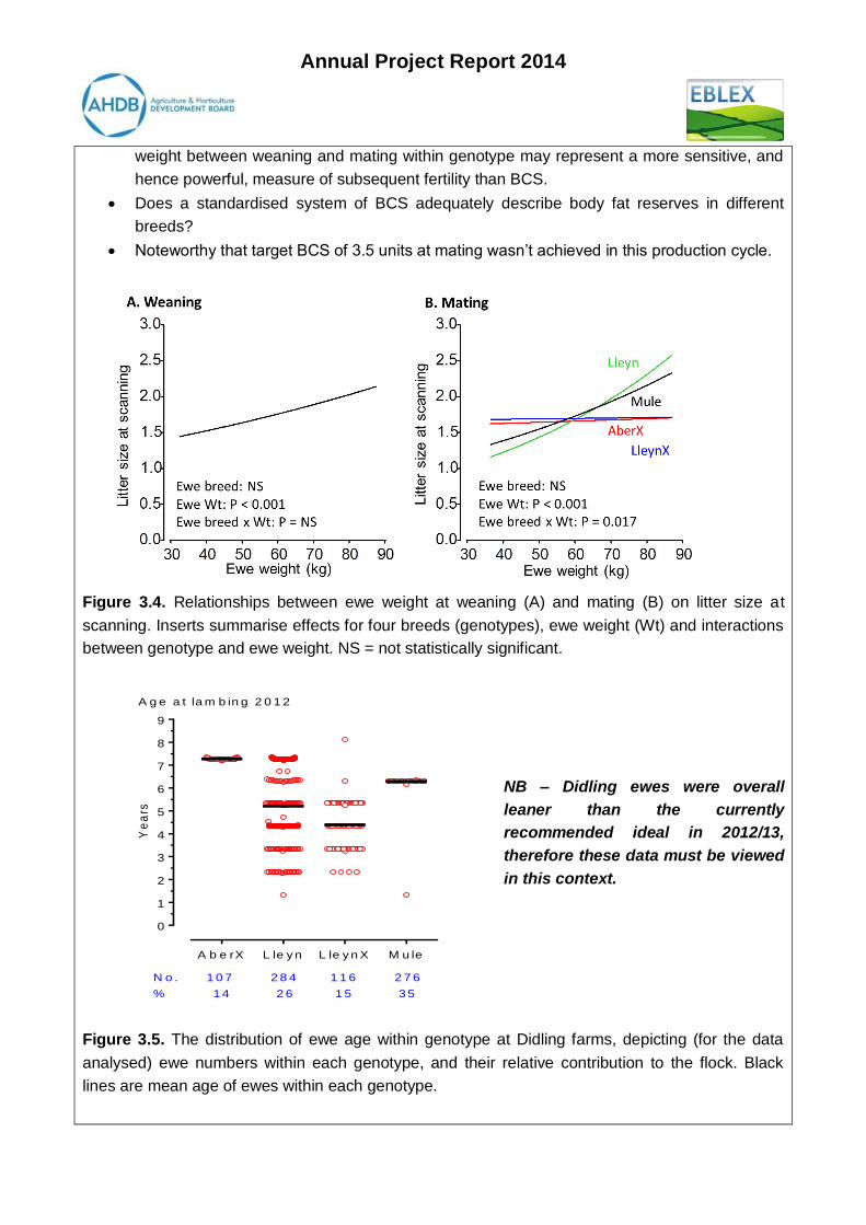
There were, however, significant positive relationships between ewe weight at both

weaning and mating in 2012 on litter size at scanning in January 2013 (Figure 3.4).

Heavier ewes (within breed) at weaning produce larger litters at scanning in the next

production cycle.

Heavier ewes at mating generally produced larger litters at scanning in the next production

cycle. Genotype by ewe weight interactions indicate that effects are not consistent across

breeds, but are evident only in Lleyns and Mules. A degree of caution is required when

interpreting these differences between genotypes as ewe age wasn’t equally represented

across breeds (Figure 3.5), and older ewes were heavier (data not shown).

Recommendation: separate analyses of effect of ewe weight and BCS for each breed

taking into consideration ewe age (where appropriate) and also mating group.

However, from the available analyses ewe weight (adjusted for age) and changes in ewe


weight between weaning and mating within genotype may represent a more sensitive, and

hence powerful, measure of subsequent fertility than BCS.

Does a standardised system of BCS adequately describe body fat reserves in different

breeds?

Noteworthy that target BCS of 3.5 units at mating wasn’t achieved in this production cycle.

Figure 3.4. Relationships between ewe weight at weaning (A) and mating (B) on litter size at

scanning. Inserts summarise effects for four breeds (genotypes), ewe weight (Wt) and interactions

between genotype and ewe weight. NS = not statistically significant.

NB – Didling ewes were overall

leaner than the currently

recommended ideal in 2012/13,

therefore these data must be viewed

in this context.

Figure 3.5. The distribution of ewe age within genotype at Didling farms, depicting (for the data

analysed) ewe numbers within each genotype, and their relative contribution to the flock. Black

lines are mean age of ewes within each genotype.

A b e rX L le y n L le y n X M u le

0

1

2

3

4

5

6

7

8

9

Ye

ars

A g e a t la m b in g 2 0 1 2

N o . 1 0 7 2 8 4 1 1 6 2 7 6

% 1 4 2 6 1 5 3 5


Impact on eight week weight and live weight gain (for lambs reared as twins) of BCS at scanning,

lambing and eight week weight (8WW) 2013, and BC change between lambing and 8WW

o “what is the impact of body condition mobilisation on lamb performance at 8WW?”


Body condition score (BCS) at scanning was positively associated with litter size at 8 weeks

following lambing (Figure 3.6). The lack of an interaction between genotype and BCS at

scanning indicates that the effect was similar for all breeds, although it appears greater for

the Lleyn and LleynX genotypes than AberX and Mules.

Figure 3.6. The relationship between ewe BCS at scanning and litter size at 8 weeks following

lambing for each of the 4 breeds (genotypes) of ewe assessed.

For ewes turned out with twin lambs, ewe BCS at scanning was not associated with lamb

weight at 8 weeks (Mean ± SEM = 39.9 ± 3.39, 39.8 ± 1.14, 40.4 ± 0.91, 40.9 ± 0.86 and

43.4 ± 1.55 kg for BCS of 1.5, 2.0, 2.5, 3.0, 3.5 units respectively). Lamb weight at 8 weeks,

however, was affected (P<0.001) by genotype (Mean ± SEM = 35.5 ± 1.47, 37.8 ± 0.92,

41.7 ± 1.22 and 44.2 ± 0.81 kg for AberX, Lleyn, LleynX and Mule ewes respectively).

For ewes turned out with twin lambs, BCS at lambing was positively associated with

combined lamb weights at 8 weeks (Figure 3.7). There were no interactions between ewe

genotype and BCS, indicating that the effect was consistent across breeds.

Similarly for ewe BCS at 8 weeks, there was a positive effect (P = 0.034) on lamb weight

(Mean ± SEM = 27.3 ± 10.9, 42.8 ± 1.19, 41.6 ± 0.67and 39.7 ± 1.05 kg for BCS of 1.0, 2.0,

2.5 and 3.0 units respectively). Clearly, however, the effect was less significant than for

ewe BCS at lambing.

Twin rearing ewes that lost most BCS between lambing and 8 weeks produced heavier

lambs at 8 weeks (Figure 3.8). This effect was consistent across breeds and indicates that

those ewes that produced the most milk (and consequently lost most condition), made the

best job or rearing their lambs.


Figure 3.7. The relationship between ewe BCS at lambing and combined lamb weight at 8 weeks

following lambing for twin suckling ewes from each of the 4 breeds (genotypes) assessed.

Figure 3.8. The relationship between ewe BCS loss from lambing to 8 weeks and combined lamb

weight at 8 weeks for twin suckling ewes from each of the 4 breeds (genotypes) assessed.

Impact on weaning weight and live weight gain (for lambs reared as twins) of BCS at lambing, eight

week weight (8WW) 2013 and weaning weight, and BC change between 8WW and weaning

o “what is the impact of body condition mobilisation on lamb performance at

weaning?”


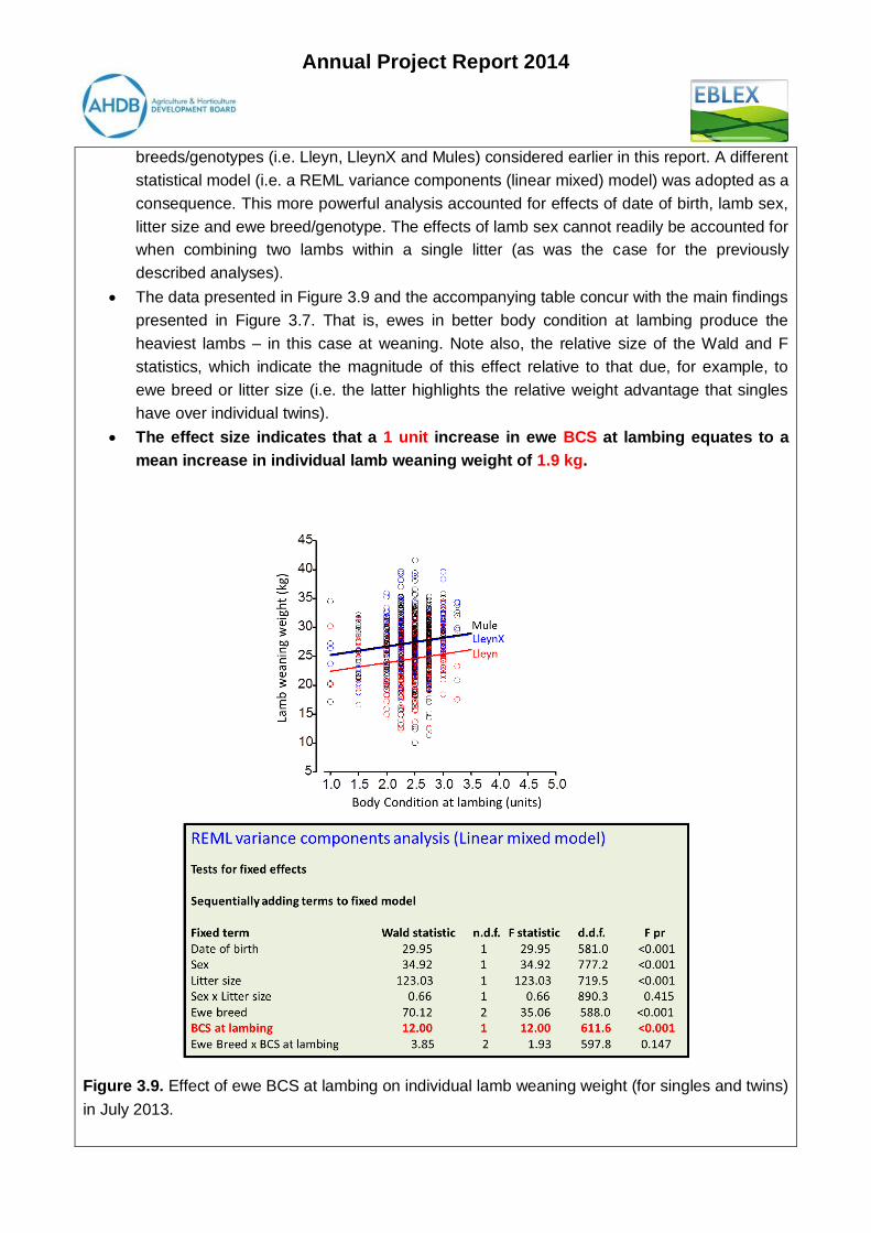
Initial analyses considered both singles and twins and focussed on just 3 of the 4


breeds/genotypes (i.e. Lleyn, LleynX and Mules) considered earlier in this report. A different

statistical model (i.e. a REML variance components (linear mixed) model) was adopted as a

consequence. This more powerful analysis accounted for effects of date of birth, lamb sex,

litter size and ewe breed/genotype. The effects of lamb sex cannot readily be accounted for

when combining two lambs within a single litter (as was the case for the previously

described analyses).

The data presented in Figure 3.9 and the accompanying table concur with the main findings

presented in Figure 3.7. That is, ewes in better body condition at lambing produce the

heaviest lambs – in this case at weaning. Note also, the relative size of the Wald and F

statistics, which indicate the magnitude of this effect relative to that due, for example, to

ewe breed or litter size (i.e. the latter highlights the relative weight advantage that singles

have over individual twins).

The effect size indicates that a 1 unit increase in ewe BCS at lambing equates to a

mean increase in individual lamb weaning weight of 1.9 kg.

Figure 3.9. Effect of ewe BCS at lambing on individual lamb weaning weight (for singles and twins)

in July 2013.


The data presented in Figure 3.10 and the accompanying table concur with the main

findings presented in Figure 3.8. That is, ewes that lose the most BCS between lambing

and 8 weeks produce the heaviest lambs – in this case at weaning. Again, note the relative

size of the Wald and F statistics, which indicate the magnitude of this effect relative to that

due, for example, to ewe breed or litter size.

Figure 3.10. Effect of change in ewe BCS between lambing and 8 weeks on individual lamb

weaning weight (for singles and twins) in July 2013.

A similar picture emerges when the data are restricted to only those ewes that were turned

out with twin lambs. Here also there was a significant (P < 0.001) effect of date-of-birth

(range spanned approximately one month).

Each day that birth was delayed during the lambing period was associated with a 0.4

kg reduction in total weaning weight per pair of lambs.

Note that the effect of date-of-birth was not statistically significant, nor nearly so profound,

at 8 weeks.

As for combined lamb weight at 8 weeks (Figure 3.7), there was a significant (P = 0.006)

effect of ewe BCS at lambing on combined lamb weaning weight (Figure 3.11), where the

effect of breed was also evident (P < 0.001).


On average, across the 4 genotypes, a 1 unit increase in ewe BCS at lambing was

associated with a 5.4 kg increase in weight of weaned lamb for twin sucking ewes.

Note – the benefit of a 1 unit increase in BCS at lambing appears to be greater for twin

suckling ewes (i.e. 5.4 kg combined lamb weight) than for the mixture of single and twin

suckling ewes (i.e. 2 x 1.9 kg combined lamb weight) depicted in Figure 3.9.

Figure 3.11. The relationship between ewe BCS at lambing and combined lamb weight at weaning

for twin suckling ewes from each of the 4 breeds (genotypes) assessed.

As for 8-week weight, twin rearing ewes that lost most BCS between lambing and 8 weeks

produced heavier lamb at weaning (Figure 3.12). Again this effect was consistent across

breeds and indicates that those ewes that produced the most milk (and consequently lost

most condition), made the best job or rearing their lambs to weaning.

Averaged across breeds the loss of 1 unit ewe BCS between lambing and 8 weeks

equated to an increase in combined weight of weaned lambs of 6.2 kg.


weight at weaning for twin suckling ewes from each of the 4 breeds (genotypes) assessed.


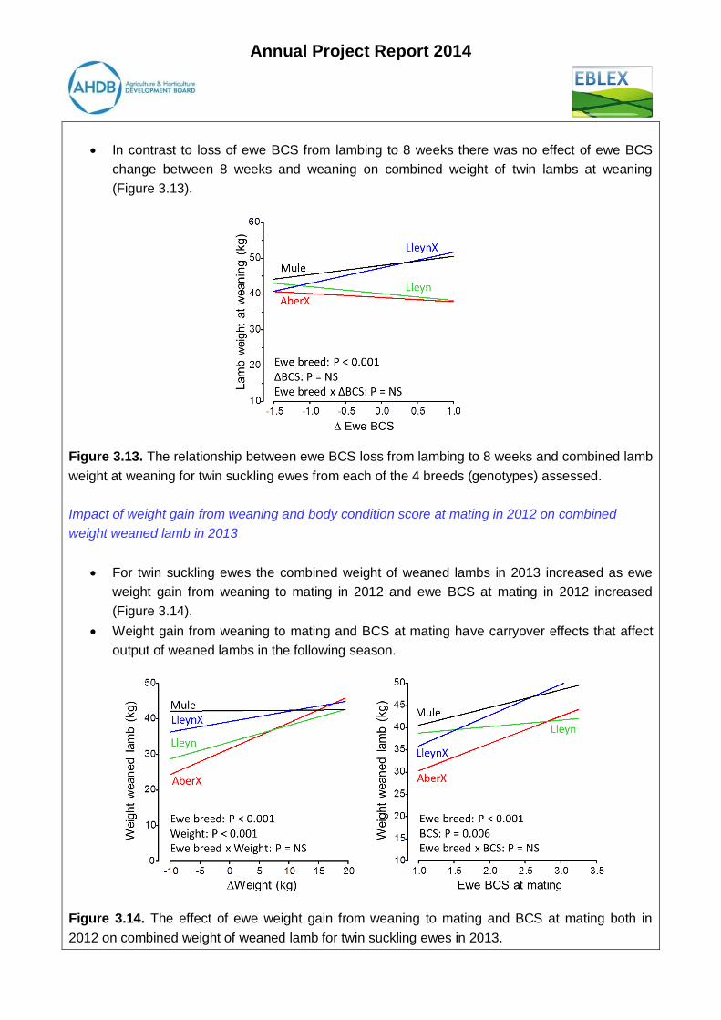
In contrast to loss of ewe BCS from lambing to 8 weeks there was no effect of ewe BCS

change between 8 weeks and weaning on combined weight of twin lambs at weaning

(Figure 3.13).


weight at weaning for twin suckling ewes from each of the 4 breeds (genotypes) assessed.

Impact of weight gain from weaning and body condition score at mating in 2012 on combined

weight weaned lamb in 2013

For twin suckling ewes the combined weight of weaned lambs in 2013 increased as ewe

weight gain from weaning to mating in 2012 and ewe BCS at mating in 2012 increased

(Figure 3.14).

Weight gain from weaning to mating and BCS at mating have carryover effects that affect

output of weaned lambs in the following season.

Figure 3.14. The effect of ewe weight gain from weaning to mating and BCS at mating both in

2012 on combined weight of weaned lamb for twin suckling ewes in 2013.


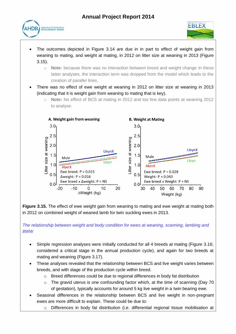
The outcomes depicted in Figure 3.14 are due in in part to effect of weight gain from

weaning to mating, and weight at mating, in 2012 on litter size at weaning in 2013 (Figure

3.15).

o Note: because there was no interaction between breed and weight change in these

latter analyses, the interaction term was dropped from the model which leads to the

creation of parallel lines.

There was no effect of ewe weight at weaning in 2012 on litter size at weaning in 2013

(indicating that it is weight gain from weaning to mating that is key).

o Note: No effect of BCS at mating in 2012 and too few data points at weaning 2012

to analyse.

Figure 3.15. The effect of ewe weight gain from weaning to mating and ewe weight at mating both

in 2012 on combined weight of weaned lamb for twin suckling ewes in 2013.

The relationship between weight and body condition for ewes at weaning, scanning, lambing and

8WW

Simple regression analyses were initially conducted for all 4 breeds at mating (Figure 3.16;

considered a critical stage in the annual production cycle), and again for two breeds at

mating and weaning (Figure 3.17).

These analyses revealed that the relationship between BCS and live weight varies between

breeds, and with stage of the production cycle within breed.

o Breed differences could be due to regional differences in body fat distribution

o The gravid uterus is one confounding factor which, at the time of scanning (Day 70

of gestation), typically accounts for around 5 kg live weight in a twin bearing ewe.

Seasonal differences in the relationship between BCS and live weight in non-pregnant

ewes are more difficult to explain. These could be due to:

o Differences in body fat distribution (i.e. differential regional tissue mobilisation at


various stages of the production cycle)

o A non-linear relationship between these parameters across a wider range of BCS

Other confounding factors include ewe age (parity).

Ewe age and litter size were considered further in more comprehensive multiple-regression

analyses summarised in Table 3.1.

Figure 3.16. Relationship between ewe BCS and live weight (kg) at mating for each of 4 breeds


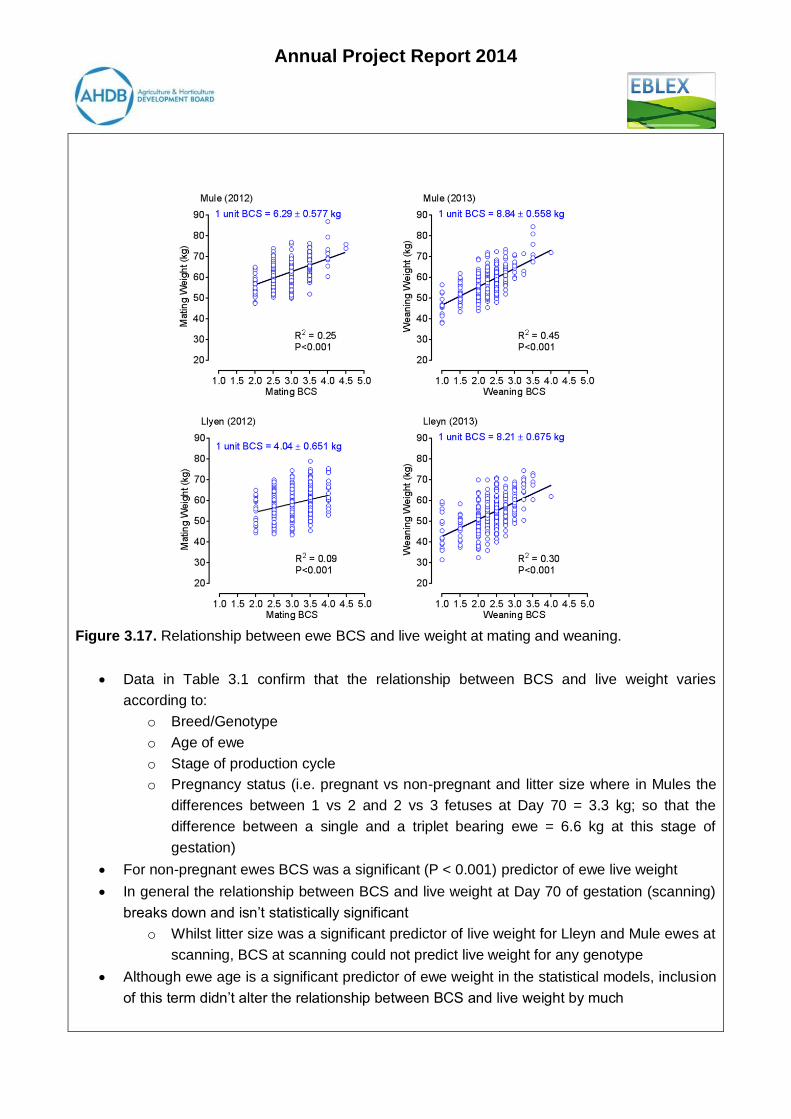
Figure 3.17. Relationship between ewe BCS and live weight at mating and weaning.

Data in Table 3.1 confirm that the relationship between BCS and live weight varies

according to:

o Breed/Genotype

o Age of ewe

o Stage of production cycle

o Pregnancy status (i.e. pregnant vs non-pregnant and litter size where in Mules the

differences between 1 vs 2 and 2 vs 3 fetuses at Day 70 = 3.3 kg; so that the

difference between a single and a triplet bearing ewe = 6.6 kg at this stage of

gestation)

For non-pregnant ewes BCS was a significant (P < 0.001) predictor of ewe live weight

In general the relationship between BCS and live weight at Day 70 of gestation (scanning)

breaks down and isn’t statistically significant

o Whilst litter size was a significant predictor of live weight for Lleyn and Mule ewes at

scanning, BCS at scanning could not predict live weight for any genotype

Although ewe age is a significant predictor of ewe weight in the statistical models, inclusion

of this term didn’t alter the relationship between BCS and live weight by much


Table 3.1. Relationship between ewe BCS and ewe live weight (kg) for different genotypes and at

different stages of the annual production cycle. Data are kg ewe live weight (± SE) per unit change

in BCS.

Genotype AberX Lleyn1 LleynX1 Mule

Stage of Cycle

Mating 4.63 ± 1.14 4.42 ± 0.69 4.39 ± 1.02

5.67 ± 0.70 4.00 ± 0.79 4.15 ± 1.04

Scanning 2.68 ± 1.34 2.92 ± 0.83 -1.31 ± 1.35 -1.76 ± 0.93

2.69 ± 1.34 3.20 ± 0.87 -1.12 ± 1.34 -1.59 ± 0.96

8 weeks 9.01 ± 2.27 8.50 ± 1.09 12.29 ± 1.90

7.76 ± 1.23 8.77 ± 1.13 12.12 ± 1.92

Weaning 9.37 ± 1.28 8.52 ± 0.74 10.75 ± 1.32

9.16 ± 0.61 7.94 ± 0.79 10.43 ± 1.35

Ewe date of birth - P < 0.001 P = 0.02 -

Litter size (scan) NS P < 0.001 NS P < 0.001

Pink rows, top line = model predictions with litter size in model, bottom row with litter size removed. Blue

columns, top line = model predictions with ewe age in model, bottom line with ewe age removed. 1 Age distribution for Lleyn and LleynX ewes only (see Figure 3.5)

Before weaning, for twin lambs growing in the top and bottom quartile of the group what are the

common factors, e.g. mobilisation of body condition, age of ewes, birth date of lamb?

A summary of the key features of 4th and 1st quartiles based on lamb growth rate from 8

weeks to weaning is provided in Figure 3.18. This period was selected because we had

weights and dates at both 8 weeks and weaning (thus able to calculate growth rates).


Figure 3.18. Features of 1st and 4th quartiles for twin lambs based on combined growth rates from

8 weeks to weaning. A, Combined growth rates during this period depicting mean date of birth

(DOB); B, Ewe breed and age distribution (numbers at base of figure refer to percentage of each

breed found in each quartile); C, Change in BCS from lambing to 8 weeks.

Note: there was a large number of missing values in these analyses because of

inconsistencies in recording between 8 weeks and weaning (e.g. lambs missed at 8 weeks

but recorded at weaning and vice versa). Data are based on records of 332 twin suckled

ewes.

Lamb date of birth was without effect on growth rate during this period.

There was no difference in the distribution of ewe genotypes between the 1st or 4th

quartiles, nor was there any difference in ewe age distribution.

1 s t Q u a r t ile 4 th Q u a r t ile

-1 0 0

0

1 0 0

2 0 0

3 0 0

4 0 0

5 0 0

B o tto m a n d to p q u a rt ile s

g/d

ay

A . T w in la m b s - c o m b in e d w e ig h t g a in

D O B 2 5 /0 3 /1 3 2 7 /0 3 /1 3

0

1

2

3

4

5

6

7

8

Ye

ars

A b e rX L le y n L le y n X M u le A b e rX L le y n L le y n X M u le

B . T w in la m b s - e w e a g e d is tr ib u tio n

1s t

Q u a rtile 4t h

Q u a rtile

1 1 .2 1 3 .4 8 .6 8 .3 5 .6 8 .5 1 4 .7 1 3 .0


-2 .5

-2 .0

-1 .5

-1 .0

-0 .5

0 .0

0 .5

1 .0

1 .5

Ch

an

ge

BC

S

P = 0 .0 3 7

C . C h a n g e B C S - la m b in g to 8 w e e k s



-1 0 0

0

1 0 0

2 0 0

3 0 0

4 0 0

5 0 0


g/d

ay

A . T w in la m b s - c o m b in e d w e ig h t g a in

D O B 2 5 /0 3 /1 3 2 7 /0 3 /1 3

0

1

2

3

4

5

6

7

8

Ye

ars

A b e rX L le y n L le y n X M u le A b e rX L le y n L le y n X M u le

B . T w in la m b s - e w e a g e d is tr ib u tio n

1s t

Q u a rtile 4t h

Q u a rtile

1 1 .2 1 3 .4 8 .6 8 .3 5 .6 8 .5 1 4 .7 1 3 .0


-2 .5

-2 .0

-1 .5

-1 .0

-0 .5

0 .0

0 .5

1 .0

1 .5

Ch

an

ge

BC

S

P = 0 .0 3 7

C . C h a n g e B C S - la m b in g to 8 w e e k s



There was a modest but statistically significant effect of body condition score change during

this period. On average, ewes in the 4th Quartile lost more (P = 0.037) BCS.

Figure 3.19. Distribution of sire breeds (genotypes) between quartiles (A) and combined growth

rate of twin lambs between sire breeds and quartiles (B). Note: 2 based on counts and not

percentages.

The main factor explaining differences in growth rate between the 1st and 4th Quartiles was

sire breed (Figure 3.19).

Lleyn lambs were the poorest growing and so didn’t feature in Q4. In contrast AberX lambs

grew well and didn’t feature prominently in Q1.

Q 1 Q 4 Q 1 Q 4 Q 1 Q 4 Q 1 Q 4 Q 1 Q 4

0

1 0

2 0

3 0

4 0

5 0

Pe

rce

nta

ge

A b e rM a x A b e rX L le yn S D X S u fte x

2 = 5 0 .2

D F = 4

P < 0 .0 0 1

A . S ire b re e d d is tr ib u tio n b e tw e e n q u a rt ile s

Q 1 Q 4 Q 1 Q 4 Q 1 Q 4 Q 1 Q 4 Q 1 Q 4

-2 5

0

2 5

5 0

7 5

1 0 0

1 2 5

1 5 0

1 7 5

2 0 0

2 2 5

2 5 0

2 7 5

3 0 0

g/d

ay

A b e rM a x A b e rX L le yn S D X S u fte x

B . S ire b re e d d is tr ib u tio n b e tw e e n q u a rt ile s

Q 1 G e n o ty p e : P < 0 .0 0 1

Q 4 G e n o ty p e : P < 0 .0 0 1

B. Combined growth rate of twin lambs between sire

breeds and quartiles


One can surmise from these analyses that neither ewe breed nor ewe age had any

significant effect of lamb growth rate from 8 weeks to weaning. Similarly, changes in body

condition score are minimal, and there was no effect of lamb age. The strong sire effect

indicates that during this period lamb growth rates were largely independent of the ewe. In

addition to the effect of sire, lamb performance probably reflects differences in herbage

availability and quality for which, at the time of analyses, we had no information.

For twin lambs in the top and bottom quartile for growth rate prior to weaning, what is the impact in

terms of slaughter age and weight?

Gareth Owen

Background to farms, summary of physical and financial performance

Seasonal variation in BCS from scanning 2013 to weaning 2013 are summarised in Figure

3.20.

o CharollaisX ewes maintained BCS throughout this period whereas Mule ewes lost a

significant (P < 0.001) amount of BCS (> 0.75 units) between lambing and weaning.

These ewes had median BCS of 1.75 units by weaning.

Ewes that were analysed fell into each of the following age categories at of lambing 2013

(Charollais: 140 x 3 years, 27 x 4 years; Mules, 556 x 3 years, 240 x 4 years, 162 x 5 years

and 120 x 6 years).

Figure 3.20. Seasonal pattern of body condition scores (BCS) for CharollaisX and Mule ewes at

Launde Abbey. Data are presented as boxplots depicting median, 25 th and 75th percentiles, with

whiskers representing 1st and 99th percentiles.

For Mule ewes BCS at lambing in 2013 decreased (P < 0.001) with age, albeit only slightly.

Among Mules, ewe age had no effect on litter size at either scanning or lambing.

Litter size was greater (P < 0.001) for Mule than for CharollaisX ewes (Figure 3.21), and

S c a n n in g L a m b in g W e a n in g

1 .0

1 .5

2 .0

2 .5

3 .0

3 .5

4 .0

Bo

dy

Co

nd

itio

n S

co

re (

un

its

)

A . C h a ro lla is X

S c a n n in g L a m b in g W e a n in g

1 .0

1 .5

2 .0

2 .5

3 .0

3 .5

4 .0

Bo

dy

Co

nd

itio

n S

co

re (

un

its

)

B . M u le s


increased (P < 0.001) with BCS at both scanning and lambing.

Mule ewes lost slightly more (P = 0.003) fetuses from scanning to lambing than CharollaisX

ewes (lambs born as a proportion of those predicted at scanning = 97.6 ± 0.63 vs 95.07 ±

0.32 % for Charollais vs Mule ewes).

On average weaning weights (across singles and twins combined) were greater (P < 0.001)

for Mule lambs than CharollaisX (40.8 ± 0.38 vs 32.8 ± 1.09 kg).

For Mule ewes output of weaned lamb = 32.3 ± 0.79, 44.0 ± 0.46 and 44.4 ± 2.47 kg for

singles, twins and triplets respectively.

Figure 3.21. Effect of genotype on litter size at scanning and lambing.

Figure 3.22. Relationship between litter size and change in ewe BCS from lambing to weaning on

weight of weaned lamb for Mule ewes.

0 .0

0 .5

1 .0

1 .5

2 .0

Lit

ter

siz

e

S ca n L a m b S ca n L a m b

C h a ro lla isX M u le

P < 0 .0 0 1


For Mules ewes there was a positive relationship between change in BCS and weight of

weaned lamb (Figure 3.22).

o Unsurprisingly the combined weight of twin lambs was greater than that for singles

o The interaction indicates that the benefits of BCS gain were greater for twin suckling

than single suckling ewes

In contrast there was no effect of ewe BCS change from lambing to weaning on weight of

weaned lamb for CharollaisX ewes (Figure 3.23).

o Again, however, as expected weight of weaned lamb was greater for twins than for

singles

o There was a suggestion that change in BCS was negatively associated with weight

of weaned lambs among twins. This would be consistent with the data from Didling

that considered BCS change from lambing to 8 weeks.

Figure 3.23. Relationship between litter size and change in BCS from lambing to weaning on

weight of weaned lamb for CharollaisX ewes.

Further analyses of data from Mule ewes revealed a positive relationship between ewe age

and weight of weaned lamb (Figure 3.24).

o That is, older ewes produced heavier lambs

o The interaction indicates that the effect of ewe age is greater for those rearing twins

than singles

These observations are significant because, as can be seen in Figure 3.25, older ewes lost

less condition, and in fact the oldest ewes gained condition, from lambing to weaning in the

Spring of 2013.

o Ewes rearing singles gained more condition (or lost less) than those rearing twins

o The interaction indicates that this effect was greater for older ewes

Collectively, these results indicate that, for Mule ewes, older dams lost less condition and

produced heavier lambs at weaning.


o This was the case for ewes rearing both singles and twins

However, older Mule ewes at Launde Abbey lambed earlier in the season (data not shown)

o Hence their lambs were older and heavier at weaning

o Ewes that lambed earlier in the season also lost less BCS from lambing to weaning

(indeed the earliest lambing ewes gained condition) (data not shown)

Figure 3.24. The relationship between ewe age and weight of weaned lamb for Mule ewes rearing

singletons and twins.

Figure 3.25. The relationship between ewe age and change in BCS for Mule ewes rearing single

and twin lambs up to weaning in 2013.


Hence older Mule ewes produced heavier lambs largely because they lambed earlier in the

season.

Why did they lose less (or gain more) BCS?

o It was noted earlier that they tended to be leaner at lambing

o Leaner Mule ewes at lambing lost less BCS after lambing (Figure 3.26)

o Consequently they could have gained BCS latterly in the period leading up to

weaning by virtue of the fact that they lambed earlier and were leaner – but there

could be other farm (i.e. grazing-field) related factors involved and which were not

considered here

o Therefore, the apparent positive relationship between BCS change and weight of

weaned lamb depicted in Figure 3.22 is not likely to be causal, but confounded by

ewe age, date of lambing and BCS at lambing

o Indeed, a multiple-regression model that sequentially included the terms ‘ewe age’,

‘lambing date’, ‘litter size’ and ‘change in ewe BCS from lambing to weaning’

indicated that BCS change was not significant in predicting weaning weight in itself,

but that there was a three-way interaction (P = 0.002) between ‘ewe age’, ‘lambing

date’, and ‘change in ewe BCS from lambing to weaning’

This is important because the older Mule ewes at Launde Abbey are comparable in age to

Mule ewes at Didling where BCS loss was associated with increased weight of twin lambs

at weaning.

o In addition the comments above the intervals (i.e. lambing to 8 weeks (Didling

analysis) vs lambing to weaning (Launde Abbey analysis)) in these separate

analyses are not comparable

Figure 3.26. The relationship between ewe BCS at lambing and change in BCS after lambing for

Mule ewes.


Malcom Sanderson, Lower Highfield Farm

Seasonal variation in BCS from mating 2012 to weaning 2013 for Mule and Texel ewes are

summarised in Figure 3.27.

o Analysis comes with a health warning in that there were numerous missing values

and some animals appeared late in the season with no previous record

o Overlap with the finishing period and ‘new’ ewes introduced to the breeding flock for

2013 mating meant that data later in the season were not included until IDs could be

confirmed.

Weight data was not included as often ewes weren’t weighed and a default value of 70 kg

was used.

Ewes were in good (close to target) BCS at mating in 2012 and generally lost a modest

amount of condition through the remainder of the production season.


M a tin g S c a n n in g 8 w e e k s W e a n in g

1

2

3

4

5B

od

y C

on

dit

ion

Sc

ore

(u

nit

s)

2 0 1 2 2 0 1 3

A . M u le e w e s

3 1 82 1 31 1 5 2 9 3

M a tin g S c a n n in g 8 w e e k s W e a n in g

1

2

3

4

5

Bo

dy

Co

nd

itio

n S

co

re (

un

its

)

2 0 1 2 2 0 1 3

B . T e x e l e w e s

1 2 69 91 3 9 1

Figure 3.27. Seasonal pattern of body condition scores (BCS) for (A) Mule and (B) Texel ewes.

Data are presented as boxplots depicting median, 25 th and 75th percentiles, with whiskers

representing 1st and 99th percentiles.

An even age distribution exists for both breeds, but Mule ewes were older (P < 0.001)

overall (Figure 3.28).


M u le s T e x e ls

0

2

4

6

8

1 0

Ag

e (

ye

ars

)

M u le T e x e l

0 .0

0 .5

1 .0

1 .5

2 .0

L itte r s iz e

P < 0 .0 0 1

Nu

mb

er

Figure 3.28. Ewe age distribution for Mule and Texel ewes at Lower Highfield. Black lines are

mean age of ewes within each genotype.

Predicted litter size at scanning was also greater for Mule than for Texel ewes (Figure 3.29)

Figure 3.29. Predicted litter size at scanning 2013 for Mule and Texel ewes at Lower Highfield.

However, there was a significant breed by ewe age interaction which indicated that litter

size increased with ewe age in Texel ewes to a greater extent than Mule ewes (Figure

3.30).

Neonatal mortality was greater (P < 0.001) for Texel ewes than for Mules and for wether

lambs than for with ewe or intact ram lambs (Figure 3.31).

The effect of castration at the time was noted to have contributed to this.

More ram lambs from young Texel ewes were castrated at birth, and this factor alone

accounts for the interaction observed between ewe breed and age on the proportion of

lambs that survived during the neonatal period (Figure 3.32).


M u le T e x e l

0 .0 0

0 .0 3

0 .0 6

0 .0 9

0 .1 2

A . N e o n a ta l m o rta lity

P < 0 .0 0 1

Pro

po

rtio

n

E w e R a m W e th e r

0

4

8

1 2

1 6

2 0

B . N e o n a ta l m o rta lity

P < 0 .0 0 1

Pro

po

rtio

n

Figure 3.30. Predicted litter size at scanning 2013 for Mule and Texel ewes at Lower Highfield,

indicting an interaction between breed and ewe age.

Figure 3.31. Neonatal mortality for (A) Mule and Texel ewes and by (B) lamb gender at lambing

2013.


Figure 3.32. Interaction between ewe breed and age on neonatal mortality (actually the proportion

of lambs that survived) at lambing 2013.

The data on lamb performance as presented will require considerable effort to align with

ewe performance data, and so these analyses remain to be conducted.

o Litter size and lamb gender also couldn’t be accounted for with the available data

This is one unit where guidance is certainly required with respect to data capture and

presentation.

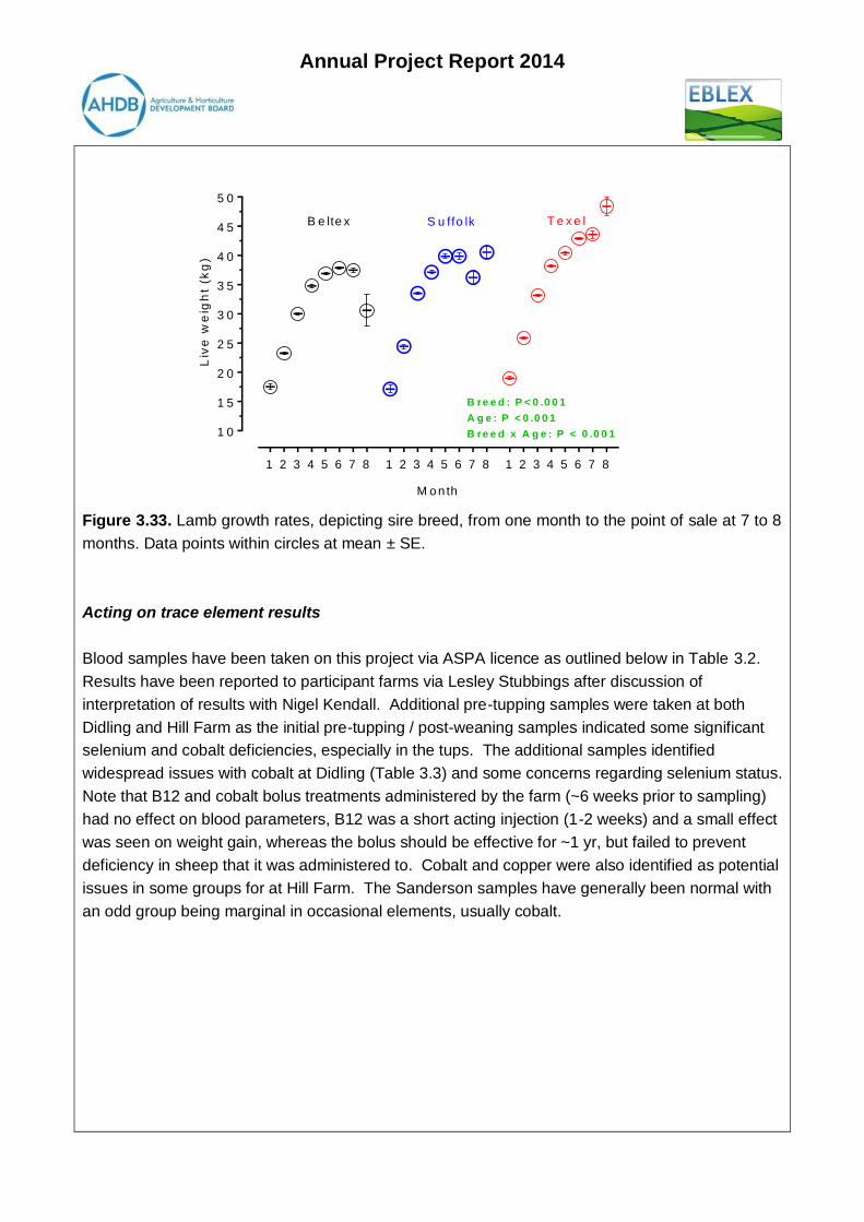
Data in Figure 3.33 illustrate lamb growth rates from one month after lambing until the point

of sale.

o Error bars increase towards the end, and live weights deviate, reflecting the

diminished group size of remaining lambs as the fittest are drafted for sale

o With respect to growth rates and weight at sale, Texel > Suffolk > Beltex


1 2 3 4 5 6 7 8 1 2 3 4 5 6 7 8 1 2 3 4 5 6 7 8

1 0

1 5

2 0

2 5

3 0

3 5

4 0

4 5

5 0

M o n th

Liv

e w

eig

ht

(kg

)

B e lte x S u ffo lk T e x e l

B re e d : P < 0 .0 0 1

A g e : P < 0 .0 0 1

B re e d x A g e : P < 0 .0 0 1

Figure 3.33. Lamb growth rates, depicting sire breed, from one month to the point of sale at 7 to 8

months. Data points within circles at mean ± SE.

Acting on trace element results

Blood samples have been taken on this project via ASPA licence as outlined below in Table 3.2.

Results have been reported to participant farms via Lesley Stubbings after discussion of

interpretation of results with Nigel Kendall. Additional pre-tupping samples were taken at both

Didling and Hill Farm as the initial pre-tupping / post-weaning samples indicated some significant

selenium and cobalt deficiencies, especially in the tups. The additional samples identified

widespread issues with cobalt at Didling (Table 3.3) and some concerns regarding selenium status.

Note that B12 and cobalt bolus treatments administered by the farm (~6 weeks prior to sampling)

had no effect on blood parameters, B12 was a short acting injection (1-2 weeks) and a small effect

was seen on weight gain, whereas the bolus should be effective for ~1 yr, but failed to prevent

deficiency in sheep that it was administered to. Cobalt and copper were also identified as potential

issues in some groups for at Hill Farm. The Sanderson samples have generally been normal with

an odd group being marginal in occasional elements, usually cobalt.


Table 3.2. Dates of blood samples. *Additional samples taken on 18 th January 2013 to address

an energy query in the housing diet. Didling has also had submitted samples taken for veterinary

purposes which were analysed under trial budget to investigate poor condition in a ram and in

some housed ewes.

Sanderson,

Lower Highfield Didling Farms, Didling Owen, Hill Farm

Post scan/pre lamb 8th January 2013 28

th February 2013 *28

th February 2013

Post lamb 11th April 2013 17

th May 2013 22

nd May 2013

Peri wean/ pre tup 3rd

July 2013 17th July 2013 15

th July 2013

Additional pre tup - 20th September 2013 11

th September 2013

Scan 3rd

January 2014 13th January 2014 14

th January 2014

Table 3.3. Cobalt status at Didling 20th September split into groups and treatments within groups,

showing numbers of samples found to be low (<188 pmol/l = AHVLA deficiency reference),

marginal 189-400 pmol/l and above marginal (>400 pmol/l).

Group Deficient

(<188)

Marginal

(189-400) >400

Tup - suftex 1 2 0

Tup - aberfield 0 3 0

Small lamb 1 3 0

Mid lamb (no treat) 1 2 0

Mid lamb (B12 inject) 2 1 0

Mid lamb (Co bolus) 2 1 0

Finishing lamb 0 0 4

Shearling aberx (B12 inject) 2 1 0

Shearling aberx (Co bolus) 1 1 1

Shearling Lleyn (B12 inject) 0 3 0

Shearling Lleyn (Co bolus) 0 3 0

Thin ewes 0 1 3

Fit ewes (off down) 1 2 1

Fit ewes (not off down) 0 2 2

Grass samples have now been taken from all three farms and show considerable variation

between fields. In general, permanent pastures are lower in selenium and cobalt than the shorter

term leys, especially at Didling and Hill Farm (Table 3.4). This is not as pronounced at

Sanderson’s. Given that selenium levels of grass at Sanderson are as low as those at Hill Farm, it

is surprising that more selenium issues have not been observed at Sanderson’s. Sanderson’s have

much higher cobalt status in the grass. Curiously, occasional issues concerning cobalt/B12 status


are seen at Sanderson’s.

Table 3.4. Selenium and cobalt status of grass samples collected from each of the three farms.

mg/kg DM Selenium Cobalt

Owen, Hill Farm 0.036-0.126 0.158-0.482

Sanderson 0.061-0.080 0.215-0.329

Didling 0.047-0.225 0.026-0.095

‘Normal’ 0.2-0.3 0.2-0.5

Summary of actions that have been taken on the farms as a results of the samples taken

Sanderson’s have continued with their routine and continue to supplement cobalt, including the

use of Smartshot injections (long acting B12) on lambs at 6-8 weeks of age.

At Didling, in light of the low cobalt status in the autumn, all ewes were put onto a cobalt

supplementations trial (Cara Campbell, MRes)

o Although this is still being analysed and written up the indications are that through the

autumn, either due to field moves or a season effect, the cobalt status increased from the

initial marginal concentrations to a sufficient status during the trial.

o However, Didling have altered the grazing/conservation strategy to manage the low cobalt

status identified. The lowest cobalt fields are being conserved to be fed out as a complete

diet TMR (with mineralisation), with other low cobalt fields having creep feeding of lambs.

Only the highest cobalt status fields are being grazed unsupplemented, the weights are

being monitored and compared to the creep fed lambs and supplements will be used if

weight gains decrease using the creep fed lambs as a guide.

At Hill Farm, ewes were initially targeted to prevent the fall off in status as seen in the lambs

with selenium and cobalt being supplemented at lambing, in the main via zinc, cobalt and

selenium soluble glass boluses with a few ewes (~6) per group being left untreated to act as

sentinels to reflect the status of the field and confirm if the additional mineral treatment had an

effect.

In addition 400 ewes have been put onto a 2x2 factoral Se-I bolus and Smartshot injection trial

(Liza Sixsmith, PhD).

In addition on both Hill farm and at Didling the poor mineral status of the tups was corrected.

It is too early to have cost benefits from this supplementation work, however the autumn

supplementation at Didling does not appear on first analysis to give any additional benefit,

probably due to the increasing status across the autumn as seen in the control group.

The ‘rescuing’ of status in the rams at both Didling and Hill farm will have given economic

benefit but it is impossible to quantify this as no group of rams was left untreated to show the

true loss of leaving these rams untreated.

Sample numbers for diagnostic tests


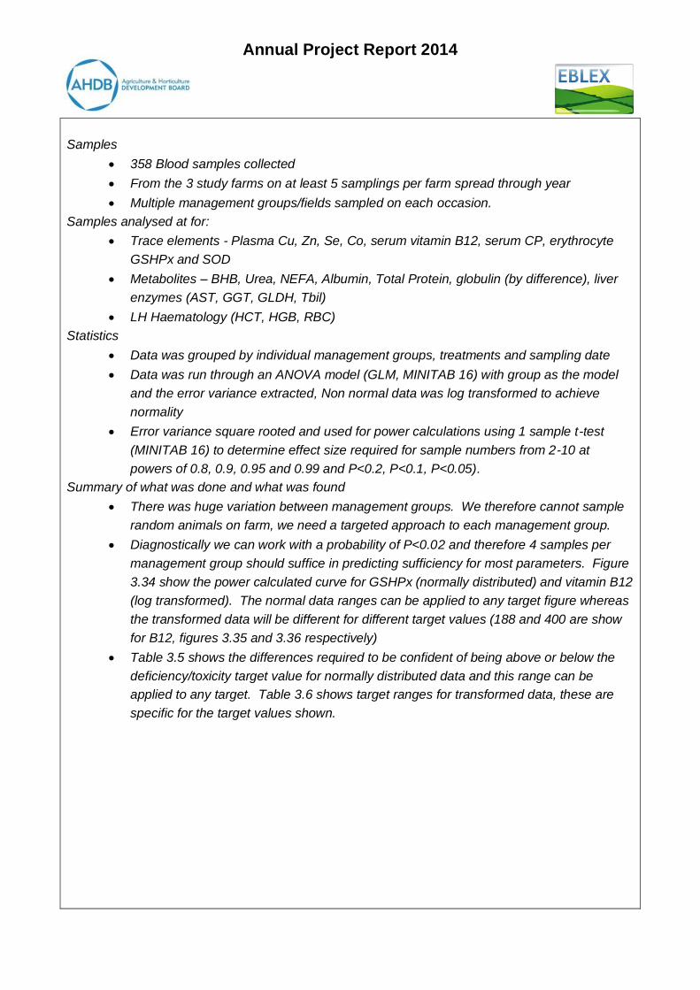
Samples

358 Blood samples collected

From the 3 study farms on at least 5 samplings per farm spread through year

Multiple management groups/fields sampled on each occasion.

Samples analysed at for:

Trace elements - Plasma Cu, Zn, Se, Co, serum vitamin B12, serum CP, erythrocyte

GSHPx and SOD

Metabolites – BHB, Urea, NEFA, Albumin, Total Protein, globulin (by difference), liver

enzymes (AST, GGT, GLDH, Tbil)

LH Haematology (HCT, HGB, RBC)

Statistics

Data was grouped by individual management groups, treatments and sampling date

Data was run through an ANOVA model (GLM, MINITAB 16) with group as the model

and the error variance extracted, Non normal data was log transformed to achieve

normality

Error variance square rooted and used for power calculations using 1 sample t-test

(MINITAB 16) to determine effect size required for sample numbers from 2-10 at

powers of 0.8, 0.9, 0.95 and 0.99 and P<0.2, P<0.1, P<0.05).

Summary of what was done and what was found

There was huge variation between management groups. We therefore cannot sample

random animals on farm, we need a targeted approach to each management group.

Diagnostically we can work with a probability of P<0.02 and therefore 4 samples per

management group should suffice in predicting sufficiency for most parameters. Figure

3.34 show the power calculated curve for GSHPx (normally distributed) and vitamin B12

(log transformed). The normal data ranges can be applied to any target figure whereas

the transformed data will be different for different target values (188 and 400 are show

for B12, figures 3.35 and 3.36 respectively)

Table 3.5 shows the differences required to be confident of being above or below the

deficiency/toxicity target value for normally distributed data and this range can be

applied to any target. Table 3.6 shows target ranges for transformed data, these are

specific for the target values shown.


Figure 3.34 The difference from target value at a power of 80%, for P<0.05,0.1,0.2 against sample

numbers for the normally distributed eGSHPx. This can be applied to any target value.

Figure 3.35 The difference from target value of 188 at a power of 80%, for P<0.05,0.1,0.2 against

sample numbers for the non-normally distributed vitamin B12.


Figure 3.36 The difference from target value of 400 at a power of 80%, for P<0.05,0.1,0.2 against

sample numbers for the non-normally distributed vitamin B12.

Although 4 is a suitable number for diagnostic purposes, for trial work where the desired

probability will be P<0.05 then a larger sample size (8-10) would be better.


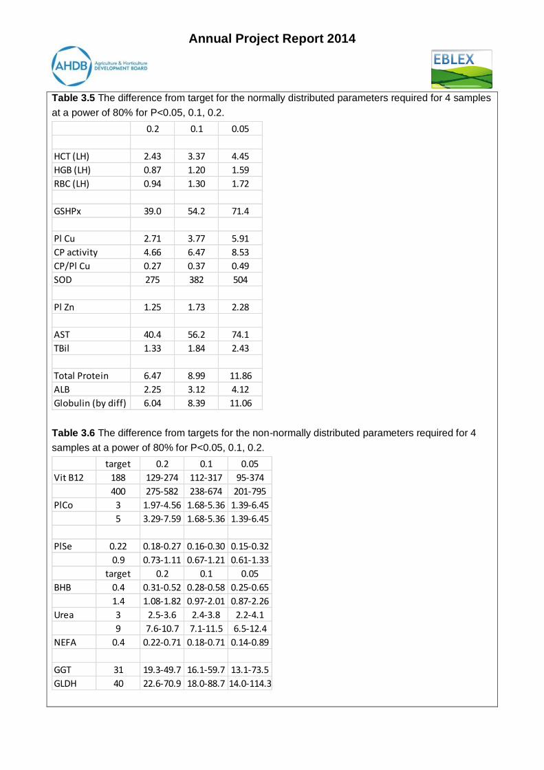
Table 3.5 The difference from target for the normally distributed parameters required for 4 samples

at a power of 80% for P<0.05, 0.1, 0.2.

Table 3.6 The difference from targets for the non-normally distributed parameters required for 4

samples at a power of 80% for P<0.05, 0.1, 0.2.

0.2 0.1 0.05

HCT (LH) 2.43 3.37 4.45

HGB (LH) 0.87 1.20 1.59

RBC (LH) 0.94 1.30 1.72

GSHPx 39.0 54.2 71.4

Pl Cu 2.71 3.77 5.91

CP activity 4.66 6.47 8.53

CP/Pl Cu 0.27 0.37 0.49

SOD 275 382 504

Pl Zn 1.25 1.73 2.28

AST 40.4 56.2 74.1

TBil 1.33 1.84 2.43

Total Protein 6.47 8.99 11.86

ALB 2.25 3.12 4.12

Globulin (by diff) 6.04 8.39 11.06

target 0.2 0.1 0.05

Vit B12 188 129-274 112-317 95-374

400 275-582 238-674 201-795

PlCo 3 1.97-4.56 1.68-5.36 1.39-6.45

5 3.29-7.59 1.68-5.36 1.39-6.45

PlSe 0.22 0.18-0.27 0.16-0.30 0.15-0.32

0.9 0.73-1.11 0.67-1.21 0.61-1.33

target 0.2 0.1 0.05

BHB 0.4 0.31-0.52 0.28-0.58 0.25-0.65

1.4 1.08-1.82 0.97-2.01 0.87-2.26

Urea 3 2.5-3.6 2.4-3.8 2.2-4.1

9 7.6-10.7 7.1-11.5 6.5-12.4

NEFA 0.4 0.22-0.71 0.18-0.71 0.14-0.89

GGT 31 19.3-49.7 16.1-59.7 13.1-73.5

GLDH 40 22.6-70.9 18.0-88.7 14.0-114.3


Q4: Discussion – what do the results mean for levy payers?

Key messages

For producers

BCS is highly repeatable and can be carried out with relative ease on commercial

premises.

Body weight is not a good proxy for BCS within a group (flock) situation and you cannot

judge BCS by eye.

Lamb growth rates are critical, in particular during the first 8 weeks - if lambs get off to a

poor start they do not compensate and remain the poorest lambs throughout the

season.

o The growth rates on all 3 farms were lower than expected and the project has

set out to improve this in 2014.

Ewe BCS is costly in terms of dry matter requirements once they become lean and if a

ewe falls below BCS 2 at weaning it can be hard to get her back to target by mating.

o Producers need to ensure that BCS gain in ewes is given adequate priority

o To establish the relative benefits of this will require monitoring ewe and lamb

performance each season over 3 or more seasons to assess long-term

cumulative effects on lamb output

High quality grazing and conserved forage can form the vast majority of the ewe (and

lambs) diet with appropriate, small levels of supplementation.

EID has huge potential for the management of commercial flocks in terms of decision

making driven by KPIs at various stages in the year.

o Our preliminary analyses of data from the pilot study would certainly support this

When assessing nutritional status, you cannot assume the samples from one group

represent the whole farm, you need to sample each management group, or at least a

large proportion of them.

Mineral supplementation is not a precise science it is an exercise in risk management.

If a supplement is required then it is better provided before a deficiency is obvious and

performance has been lost.

Decisions to supplement should be based on inputs such as forage mineral profile,

grass mineral profiles, animal performance and direct assessment of animal status. As

we have mentioned that it is better to supplement before a clinical effect on

performance and risk management on a farm can include previous years data

particularly performance and animal status measurement.

Farmers need to make sure that rams have their mineral status monitored at least 8

weeks prior to the start of tupping as this proved to be a large issue on 2 of the 3 farms.

They also need to be aware of breed differences in mineral status which were carried

forward in terms of performance.


For the research team, e.g. regarding the process

Many of the above also apply to the researchers. In addition:

EID offers the potential to collect large volumes of highly valuable data which can be of

immediate benefit to the producer and long-term benefit to the extension officer.

o Systems of data capture and processing need to be developed and refined so that

data can be quickly and easily analysed

o Failure to achieve this will dissuade producers from taking full advantage of what

EID and precision farming technologies have to offer.

BCS is relatively easy for farmers to learn and apply accurately and it is highly repeatable

o However, for the research team we need to establish optimal BCS for different

breeds – reflecting probable differences in fat distribution between breeds.

o Where EID and automated systems are in place it may be worth re-evaluating live

weight measurements (at least in non-pregnant ewes), and revisit relationships

between live weight and BCS for different breeds.

o This can & should be done on an individual ewe basis looking at changes over time.

Live weight changes associated with one unit of BCS change are not constant between breeds,

and differ with ewe age and pregnancy status

o The relationship between BCS and level of body fatness has never fully been

quantified in sheep and differences between breeds remain to be determined

We show that eight-week weight and weaning weights are correlated to ewe BCS and BCS

changes at mating, scanning and lambing.

Data analyses in this report are from a single season. Final conclusions can only be reached

when data from 2 or more seasons are pooled. Responses between years may vary

according to levels of BCS attained at key stages of the annual production cycle (e.g. mating,

lambing), and with growing conditions during each grazing period.

o To illustrate this point – at Didling in 2013 – it was evident that the main drivers for

lamb growth from 8 weeks to weaning was sire breed and probably the amount of

accessible quality grass.

o However, in 2014 this may be more or less evident. Dangerous to make universal

conclusions from a single season.

The major message in terms of assessing nutritional status is the variability between different

management groups on the same farm and the importance of assessing multiple groups.

The results have further confirmed our opinion that mineral supplementation needs to be an

exercise in risk management, i.e. is the likelihood of losses from a deficiency (e.g. in

performance), greater than the cost of treatment (remembering to include the length of efficacy


of each treatment considered into this calculation), if so then it is a good option to

treat/supplement.

The use of grass samples as indicators looked interesting but requires further validation work to

determine how many samples are required during the season, whether time of the year affects

grass mineral status and how these relate to sheep grazing these pastures.

Breed differences were found to exist, especially for selenium and cobalt of groups of tups

managed as one mob.

Key messages for industry

Following the pilot year the overarching message must be that BCS is a valuable tool in terms

of sheep management.

o It is easy to learn and highly repeatable and can be used to drive decisions

regarding ewe management and has direct effects on productivity.

The major message to industry in terms of nutritional monitoring is the recommendation of

sample numbers for diagnostic purposes

o 4 per management group/animal type are needed, ie ewes and lambs on the same

pasture would count as two groups.

o This does mean that to get a good ‘picture’ of the farm a relatively large number of

samples will be required but these should be used along with other indicators

(forage/grass mineral analysis) to manage mineral imbalance risks.

There is a hint that permanent pastures are poorer in cobalt and selenium status and short term

leys poorer in terms of copper status, but this needs more work.

There were also breed effects on selenium and cobalt status, breed effects on copper status

have long been known, but this may mean different breeds are more suited to the farms natural

mineral profile.

Q5: New knowledge – what key bit of new knowledge that has come out of this project?

The pilot study demonstrates that changes in BCS have longer-term effects on ewe and lamb

performance than previously appreciated.

o These effects present as a complex interaction of a number of factors many with

longitudinal implications.

Initial analyses would support the concept that BCS at specific stages of the annual production

cycle can serve as a KPI.

Variation between management groups in terms of mineral status on a single farm was most

evident in the Pilot study.

o This has implications for monitoring and risk management

Differences between breeds in selenium and cobalt status when managed together.

The recommended number of samples per ‘group’ for nutritional diagnosis is 4.


Q6: Gaps in knowledge – what gaps in knowledge did this project identify?

In no particular order:

Ewe dry matter intakes on high quality TMRs – the project suggests they are much higher than

the ‘book’ values published.

The ‘phenotypic’ mature body weight of ewes is influenced by the rearing phase to a greater

extent than previously realised and this may be at least as important as genotype.

Only after the project has run for another two seasons will we be able to pull these data out

from replacements joining the flock, where we have their joining body weights and BCS.

EID has huge potential, but there is a gap in terms of handling the data as a decision support

tool on farm on a day-to-day basis. Going forward, the project will seek to address this,

working with software providers (Border Software and Shearwell Data).

Although BCS is easily measurable, it is still subjective and with automated weighing systems

the potential of using live weight change in addition to BCS as a tool for monitoring

performance and ewe status should be evaluated.

A further gap, is the interaction between forage type and sheep mineral status, and the

seasonality of this effect.

o i.e. can we use grass mineral profiling to determine supplement requirements and

the optimal timing of supplementation?

There is a still a need to define ‘diagnostic’ ranges for productivity rather than deficiency.

There is still a need to determine the relative efficacy of different mineral supplementation

products and protocols.

Breed effects, particularly with respect of selenium and cobalt, require further investigation.


Q7: Cost: benefit – what is value of this project?

It is too early to be specific in terms of cost benefits because this report only covers the baseline

pilot year. However, we do have enough information on which to make a couple of general

calculations to illustrate the potential:

A 1% increase in the number of lambs reared on these farms will add 80p/ewe to the output

(£80/lamb). For example two of the farms are on course to increase the % lambs reared in

2014 by >25% which will add £20/ewe to the output with very little in terms of extra costs.

The analysis of the Didling data suggest that an increase in 1 unit of BCS at lambing resulted

in 5.4kgs more weight (twins combined) at weaning, equivalent to just over 30g DLWG. Faster

lamb growth rate reduces the dry matter requirement for lambs to reach the same weight. For

example at 100g/day a lamb will eat twice as much dry matter to get to the same weight as a

lamb growing at 300g/day. The net benefit to the farmer is firstly lambs finishing quickly, at

better prices, but also the scope to keep more ewes on the same area or where ewe BCS has

been a challenge, to make sure the ewes and lambs are not competing.

Q8: Additional deliverables – what activity is planned with the results from this project?

Activity What is planned? When likely to happen?

Events English Progressive Sheep

Group

10th July 2014 @ Didling

Press articles

Conference presentations,

papers or posters

BSAS April 2014 Some data used to support

LAS paper

Scientific papers Paper on sample numbers

2014/15

Other Sample numbers to be

presented at EBLEX

consultants day

8th July 2014

Other

sheep kpi validation project

Documents