short recap - dbs.ifi.lmu.de · • we had several appearances ofthe curse ofdimensionality: –...

DATABASESYSTEMSGROUP

Short Recap

• We had several appearances of the curse of dimensionality:– Concentration of distances

=> meaningless similarity/distance/neighborhood concept=> instability of neighborhoods

– Growing hypothesis space=> interpretation of models=> efficiency

– Empty Space Phenomenon=> impact on volume queries (rang queries, hypercube queries, …)=> importance of tails of distributions=> impact on sample sizes

• Some are due to irrelevant attributes=> get rid of irrelevant attributes, keep the redundant one

• Some are instead of relevant attributes=> among the relevant attributes, get rid of redundant attributes

Knowledge Discovery in Databases II: High‐Dimensional Data 40


Outline

1. Introduction to Feature Spaces

2. Challenges of high dimensionality

3. Feature Selection

4. Feature Reduction and Metric Learning

5. Clustering in High‐Dimensional Data



Feature selection

• A task to remove irrelevant and/or redundant features– Irrelevant features:

• Not useful for a given task• Probably decrease accuracy

– Redundant features: • Redundant feature in the presence of another relevant feature with which it is strongly

correlated• It does not drop the accuracy but may drop efficiency, explainability, …

• Deleting irrelevant and redundant features can improve the quality as well as the efficiency of the methods and the found patterns.

• New feature space: Delete all useless features from the original feature space.

• Feature selection ≠ Dimensionality reduction • Feature selection ≠ Feature extraction



Irrelevant and redundant features (unsupervised learning case)

• Irrelevance • Redundancy


Feature y is irrelevant, because if we omit x, we have only one cluster, which is uninteresting.

Features x and y are redundant, because x provides (appr.) the same information as feature y with regard to discriminating the two clusters

Source: Feature Selection for Unsupervised Learning, Dy and Brodley, Journal of Machine Learning Research 5 (2004)


Irrelevant and redundant features (supervised learning case)

• Irrelevance

• Redundancy


Feature y separates well the two classes.Feature x is irrelevant.Its addition “destroys” the class separation.

Features x and y are redundant.

Source: http://www.kdnuggets.com/2014/03/machine‐learning‐7‐pictures.html

• Individually irrelevant, together relevant


Problem definition

• Input: Vector space F =d1×..× dn with dimensions D ={d1,,..,dn}.• Output: a minimal subspace M over dimensions D` D which is optimal for a

giving data mining task.– Minimality increases the efficiency, reduces the effects of the curse of

dimensionality and increases interpretability.

Challenges:• Optimality depends on the given task• There are 2d possible solution spaces (exponential search space)• This search space is similar to the frequent item set mining problem, but:

– There is often no monotonicity in the quality of subspace (which could be used for efficient searching)

– Features might only be useful in combination with certain other features

For many popular criteria, feature selection is an exponential problem Most algorithms employ search heuristics



2 main components

1. Feature subset generation– Single dimensions– Combinations of dimensions (subpaces)

2. Feature subset evaluation– Importance scores like information gain, χ2

– Performance of a learning algorithm



Feature selection methods 1/4

• Filter methods Explores the general characteristics of the data, independent of the learning

algorithm.

• Wrapper methods– The learning algorithm is used for the evaluation of the subspace

• Embedded methods– The feature selection is part of the learning algorithm




• Filter methods– Basic idea: assign an ``importance” score to each feature to filter out the

useless ones– Examples: information gain, χ2‐statistic, TF‐IDF for text– Disconnected from the learning algorithm. – Pros:

o Fast and generic (or better say: “generalizing”)o Simple to apply

– Cons: o Doesn’t take into account interactions between featureso Individually irrelevant features, might be relevant togethero Too generic?




• Wrapper methods– A learning algorithm is employed and its performance is used to determine

the quality of selected features.– Pros:

o the ability to take into account feature dependencieso interaction between feature subset search and model selection

– Cons: o higher risk of overfitting than filter techniqueso very computationally intensive, especially if building the classifier has a high computational cost.




• Embedded methods– Such methods integrate the feature selection in model building– Example: decision tree induction algorithm: at each decision node, a

feature has to be selected.

– Pros:

o less computationally intensive than wrapper methods.

– Cons: o specific to a learning method



Search strategies in the feature space

• Forward selection– Start with an empty feature space and add relevant features

• Backward selection– Start with all features and remove irrelevant features

• Branch‐and‐bound– Find the optimal subspace under the monotonicity assumption

• Randomized– Randomized search for a k dimensional subspace

• …



Selected methods in this course

1. Forward Selection and Feature Ranking– Information Gain , 2‐Statistik, Mutual Information

2. Backward Elimination and Random Subspace Selection– Nearest‐Neighbor criterion, Model‐based search

– Branch and Bound Search

3. k‐dimensional subspace projections– Genetic Algorithms for Subspace Search– Feature Clustering for Unsupervized Problems



1. Forward Selection and Feature Ranking

Input: A supervised learning task– Target variable C– Training set of labeled feature vectors <d1, d2, …, dn>

Approach• Compute the quality q(di ,C) for each dimension di {d1,,..,dn} to predict the

correlation to C• Sort the dimensions d1,,..,dn w.r.t. q(di ,C)• Select the k‐best dimensions

Assumption: Features are only correlated via their connection to C

=> it is sufficient to evaluate the connection between each single feature d and the target variable C



Statistical quality measures for features

How suitable is feature d for predicting the value of class attribute C?

Statistical measures :• Rely on distributions over feature values and target values.

– For discrete values: determine probabilities for all value pairs.– For real valued features:

• Discretize the value space (reduction to the case above)• Use probability density functions (e.g. uniform, Gaussian,..)

• How strong is the correlation between both value distributions?• How good does splitting the values in the feature space separate values in the

target dimension?• Example quality measures:

– Information Gain– Chi‐square χ2‐statistics– Mutual Information



Information Gain 1/2

• Idea: Evaluate class discrimination in each dimension (Used in ID3 algorithm)• It uses entropy, a measure of pureness of the data

• The information gain Gain(S,A) of an attribute A relative to a training set S measures the gain reduction in S due to splitting on A:

• For nominal attributes: use attribute values

• For real valued attributes: Determine a splitting position in the value set.


)(

)(||||)(),(

AValuesvv

v SEntropySSSEntropyASGain

Before splitting After splitting on A

(pi : relative frequency of class ci in S)

k

iii ppSEntropy

12 )(log)(


Entropy (reminder)

• Let S be a collection of positive and negative examples for a binary classification problem, C={+, ‐}.

• p+: the percentage of positive examples in S• p‐: the percentage of negative examples in S• Entropy measures the impurity of S:

• Examples :– Let S: [9+,5‐]

– Let S: [7+,7‐]

– Let S: [14+,0‐]

• Entropy = 0, when all members belong to the same class• Entropy = 1, when there is an equal number of positive and negative examples

Knowledge Discovery in Databases I: Classification 56

)(log)(log)( 22 ppppSEntropy

940.0)145(log

145)

149(log

149)( 22 SEntropy

1)147(log

147)

147(log

147)( 22 SEntropy

0)140(log

140)

1414(log

1414)( 22 SEntropy

in the general case (k‐classification problem)

k

iii ppSEntropy

12 )(log)(


Information Gain 2/2

• Which attribute, “Humidity” or “Wind” is better?

• Larger values better!



Chi‐square χ2 statistics 1/2

• Idea: Measures the independency of a variable from the class variable.• Contingency table

– Divide data based on a split value s or based on discrete values

• Example: Liking science fiction movies implies playing chess?

• Chi‐square χ2 test


c

i

r

j ij

ijij

eeo

1 1

22 )(

oij:observed frequency eij: expected frequency n

hhe ji

ij

Play chess Not play chess Sum (row)Like science fiction 250 200 450

Not like science fiction 50 1000 1050

Sum(col.) 300 1200 1500

Class attribute

Pred

ictor a

ttrib

ute


Chi‐square χ2 statistics 2/2

• Example

• χ2 (chi‐square) calculation (numbers in parenthesis are expected counts calculated based on the data distribution in the two categories)

• Larger values better!


Play chess Not play chess Sum (row)Like science fiction 250 (90) 200 (360) 450

Not like science fiction 50 (210) 1000 (840) 1050

Sum(col.) 300 1200 1500

Class attributePred

ictor a

ttrib

ute

93.507840

)8401000(360

)360200(210

)21050(90

)90250( 22222


Mutual Information (MI)

Yy Xx ypxp

yxpyxpYXI)()(),(log),(),(

Y X

dxdyypxp

yxpyxpYXI)()(

),(log),(),(


• In general, MI between two variables x, y measures how much knowing one of these variables reduces uncertainty about the other

• In our case, it measures how much information a feature contributes to making the correct classification decision.

• Discrete case:

• Continuous case:

• In case of statistical independence: – p(x,y)= p(x)p(y) log(1)=0– knowing x does not reveal anything about y

p(x,y): the joint probability distribution functionp(x), p(y): the marginal probability distributions

Relation to entropy


Forward Selection and Feature Ranking ‐overview

Advantages:• Efficiency: it compares {d1, d2, …, dn} features to the class attribute C instead of

subspaces

• Training suffices with rather small sample sets

Disadvantages: • Independency assumption: Classes and features must display a direct

correlation. • In case of correlated features: Always selects the features having the strongest

direct correlation to the class variable, even if the features are strongly correlated with each other.(features might even have an identical meaning)

Knowledge Discovery in Databases II: High‐Dimensional Data

kn

61




2. Backward Elimination and Random Subspace Selection– Nearest‐Neighbor criterion, Model‐based search– Branch and Bound Search

3. k‐dimensional projections– Genetic Algorithms for Subspace Search– Feature Clustering for Unsupervized Problems



2. Backward Elimination

Idea: Start with the complete feature space and delete redundant features

Approach: Greedy Backward Elimination1. Generate the subspaces R of the feature space F2. Evaluate subspaces R with the quality measure q(R)3. Select the best subspace R* w.r.t. q(R)4. If R* has the wanted dimensionality, terminate

else start backward elimination on R*.

Applications: • Useful in supervised and unsupervised setting

– in unsupervised cases, q(R) measures structural characteristics

• Greedy search if there is no monotonicity on q(R)=> for monotonous q(R) employ branch and bound search



Distance‐based subspace quality

• Idea: Subspace quality can be evaluated by the distance between the within‐class nearest neighbor and the between‐classes nearest neighbor

• Quality criterion:For each o D, compute the closest object having the same class NNC(o) (within‐class nearest neighbor) and the closest object belonging to another class NNKC(o) (between‐classes nearest neighbor) where C = class(o).

Quality of subspace U:

• Remark: q(U) is not monotonous.By deleting a dimension, the quality can increase or decrease.

Do

U

UCK

oNNoNN

DUq

C)()(

||1)(



Model‐based approach

• Idea: Directly employ the data mining algorithm to evaluate the subspace.• Example: Evaluate each subspace by training a Naive Bayes classifier

Practical aspects:• Success of the data mining algorithm must be measurable

(e.g. class accuracy)• Runtime for training and applying the classifier should be low• The classifier parameterization should not be of great importance• Test set should have a moderate number of instances



Backward Elimination ‐ overview

Advantages:• Considers complete subspaces (multiple dependencies are used)• Can recognize and eliminate redundant features

Disadvantages:• Tests w.r.t. subspace quality usually requires much more effort• All solutions employ heuristic greedy search which do not necessarily find the

optimal feature space.



Backward elimination: Branch and Bound Search


• Given: A classification task over the feature space F.• Aim: Select the k best dimensions to learn the classifier.• Backward elimination approach “Branch and Bound”, by Narendra and

Fukunaga, 1977 is guaranteed to find the optimal feature subset under the monotonicity assumption

• The monotonicity assumption states that for two subsets X, Y and a feature selection criterion function J, if:

• E.g. X={d1,d2}, Y={d1,d2,d3} • Branch and Bound starts from the full set and removes features using a depth‐

first strategy– Nodes whose objective function are lower than the current best are not explored

since the monotonicity assumption ensures that their children will not contain a better solution.

Slide adapted from: http://courses.cs.tamu.edu/rgutier/cs790_w02/l17.pdf

⊂ ⇒ J X J Y


Example: Branch and Bound Search 1/8

Example: Original dimensionality 4, <A,B,C,D>. Target dimensionality d = 1. selected feature removed feature

(All)=0.0


A B C D//Start from the full set




(All)=0.0


A B C D

//Generate subspaces

IC (BCD)=0.0 IC(ACD)=0.015 IC(ABD)=0.021 IC(ABC)=0.03




(All)=0.0


A B C D//Choose the best one and generate its subspaces


IC(CD)=0.015 IC (BC)=0.1IC (BD)=0.1




(All)=0.0


A B C D

//Choose the best one and generate its subspaces


IC(CD)=0.015 IC (BC)=0.1IC (BD)=0.1

IC(D)=0.02 IC(C)=0.03

aktBound = 0.02

//Desired dimensionality reached, what is the bound?




(All)=0.0


A B C D


IC(CD)=0.015 IC (BC)=0.1IC (BD)=0.1

IC(D)=0.02 IC(C)=0.03

aktBound = 0.02

//Backward elimination using the bound

IC(BD) >aktBound stop branchingIC(BC) >aktBound stop branching




(All)=0.0


A B C D


IC(CD)=0.015 IC (BC)=0.1IC (BD)=0.1

IC(D)=0.02 IC(C)=0.03

aktBound = 0.02


IC(ACD) <aktBound do branchingIC(AD)>aktBound stop branchingIC(AC)>aktBound stop branching

IC(AC)=0.03IC (AD)=0.1




(All)=0.0


A B C D


IC(CD)=0.015 IC (BC)=0.1IC (BD)=0.1

IC(D)=0.02 IC(C)=0.03

aktBound = 0.02


IC(ABD)>aktBound stop branchingIC(ABC)>aktBound stop branching

IC(AC)=0.03IC (AD)=0.1


Backward elimination: Branch and Bound Search

Given: A classification task over the feature space F.Aim: Select the k best dimensions to learn the classifier.

Backward‐Elimination based in Branch and Bound:FUNCTION BranchAndBound(Featurespace F, int k)

queue.init(ASCENDING);queue.add(F, quality(F))curBound:= INFINITY;WHILE queue.NotEmpty() and aktBound > queue.top() DO

curSubSpace:= queue.top();FOR ALL Subspaces U of curSubSpace DO

IF U.dimensionality() = k THENIF quality(U)< curBound THEN

curBound := quality(U);BestSubSpace := U;

ELSEqueue.add(U, quality(U));

RETURN BestSubSpace



Subspace Inconsistency (IC)

• Idea: Having identical vectors u ,v ( vi = ui 1 i d) in subspace U but the class labels are different (C(u) C(v) ) the subspace displays an inconsistent labeling

• Measuring the inconsistency of a subspace U– XU(A): Amount of all identical vectors A in U– XcU(A): Amount of all identical vectors in U having class label C

• ICU(A): inconsistency w.r.t. A in U

Inconsistency of U:

Monotonicity:

)(max)()( AXAXAIC cUCcUU

||

)()(

DB

AICUIC DBA

U

)()( 2121 UICUICUU



Branch and Bound search ‐ overview

Advantage:• Monotonicity allows efficient search for optimal solutions• Well‐suited for binary or discrete data

(identical vectors are very likely with decreasing dimensionality)

Disadvantages:• Useless without groups of identical features (real‐valued vectors)• Worse‐case runtime complexity remains exponential in d





2. Backward Elimination and Random Subspace Selection– Nearest‐Neighbor criterion, Model‐based search

– Branch and Bound Search

3. k‐dimensional projections– Genetic Algorithms for Subspace Search– Feature Clustering for Unsupervised Problems



k‐dimensional projections

• Idea: Select n random subspaces having the target dimensionality k out of thepossible subspaces and evaluate each of them.

• Application:– Needs quality measures for complete subspaces – Trade‐off between quality and effort depends on k.

• Disadvantages: – No directed search for combining well‐suited and non‐redundant features.– Computational effort and result strongly depend on the used quality measure and

the sample size.

• Randomization approaches– Genetic algorithms– k‐medoids feature clustering

Knowledge Discovery in Databases II: High‐Dimensional Data

kd

79


Genetic Algorithms

• Idea: Randomized search through genetic algorithmsGenetic Algorithms: • Encoding of the individual states in the search space: bit‐strings • Population of solutions := set of k‐dimensional subspaces• Fitness function: quality measure for a subspace• Operators on the population:

– Mutation: dimension di in subspace U is replaced by dimension dj with a likelihood of x%

– Crossover: combine two subspaces U1, U2

o Unite the features sets of U1 and U2. o Delete random dimensions until dimensionality is k

• Selection for next population: All subspaces having at least a quality of y% of the best fitness in the current generation are copied to the next generation.

• Free tickets: Additionally each subspace is copied into the next generation with a probability of u%.



Genetic Algorithm: Schema

Generate initial populationWHILE Max_Fitness > Old_Fitness DO

Mutate current populationWHILE nextGeneration < PopulationSize DO

Generate new candidate from pairs of old subspacesIF K has a free ticket or K is fit enough THEN

copy K to the next generationRETURN fittest subspace



Genetic Algorithms

Remarks: • Here: only basic algorithmic scheme (multiple variants)• Efficient convergence by “Simulated Annealing”

(Likelihood of free tickets decreases with the iterations)Advantages:• Can escape from local extreme values during the search• Often good approximations for optimal solutionsDisadvantages:• Runtime is not bounded can become rather inefficient• Configuration depends on many parameters which have to be tuned to achieve

good quality results in efficient time



Feature‐clustering

Given: A feature space F and an unsupervised data mining task.Target: Reduce F to a subspace of k (original) dimensions while reducing

redundancy.

Idea: Cluster the features in the space of objects and select one representative feature for each of the clusters.(This is equivalent to clustering in a transposed data matrix)

Typical example: item‐based collaborative filtering


Susan 5 2 5 5 4 1

Bill 3 3 2 1 1 1

Jenny 5 4 1 1 1 4

Tim 2 2 4 5 3 3

Thomas 2 1 3 4 1 4

1 (Titanic) 2 (Braveheart) 3 (Matrix) 4 (Inception) 5 (Hobbit) 6 (300)


Feature‐clustering

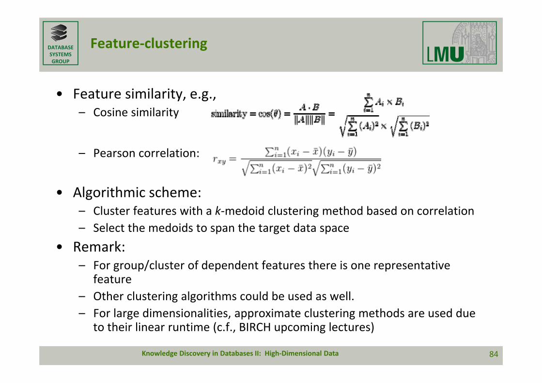
• Feature similarity, e.g.,– Cosine similarity

– Pearson correlation:

• Algorithmic scheme: – Cluster features with a k‐medoid clustering method based on correlation– Select the medoids to span the target data space

• Remark: – For group/cluster of dependent features there is one representative

feature– Other clustering algorithms could be used as well.– For large dimensionalities, approximate clustering methods are used due

to their linear runtime (c.f., BIRCH upcoming lectures)



Feature‐Clustering based on correlation

Advantages:• Depending on the clustering algorithm quite efficient• Unsupervised method

Disadvantages:• Results are usually not deterministic (partitioning clustering)• Representatives are usually unstable for different clustering methods and

parameters.• Based on pairwise correlation and dependencies

=> multiple dependencies are not considered



Feature selection: overview

• Forward‐Selection: Examines each dimension D‘ {D1,,..,Dd}. and selects the k‐best to span the target space.– Greedy Selection based on Information Gain, 2 Statistics or Mutual Information

• Backward‐Elimination: Start with the complete feature space and successively remove the worst dimensions.– Greedy Elimination with model‐based and nearest‐neighbor based approaches– Branch and Bound Search based on inconsistency

• k‐dimensional Projections: Directly search in the set of k‐dimensional subspaces for the best suited– Genetic algorithms (quality measures as with backward elimination)– Feature clustering based on correlation



Feature selection: discussion

• Many algorithms based on different heuristics• There are two reason to delete features:

– Redundancy: Features can be expressed by other features.– Missing correlation to the target variable

• Often even approximate results are capable of increasing efficiency and quality in a data mining tasks

• Caution: Selected features need not have a causal connection to the target variable, but both observation might depend on the same mechanisms in the data space (hidden variables).

• Different indicators to consider in the comparison of before and after selection performance– Model performance, time, dimensionality, …



Further literature on feature selection

• I. Guyon, A. Elisseeff: An Introduction to Variable and Feature Selection, Journal of Machine Learning Research 3, 2003.

• H. Liu and H. Motoda, Computations methods of feature selection, Chapman & Hall/ CRC, 2008.

• A.Blum and P. Langley: Selection of Relevant Features and Examples in Machine Learning, Artificial Intelligence (97),1997.

• H. Liu and L. Yu: Feature Selection for Data Mining (WWW), 2002. • L.C. Molina, L. Belanche, Â. Nebot: Feature Selection Algorithms: A Survey and

Experimental Evaluations, ICDM 2002, Maebashi City, Japan.• P. Mitra, C.A. Murthy and S.K. Pal: Unsupervised Feature Selection using Feature

Similarity, IEEE Transacitons on pattern analysis and Machicne intelligence, Vol. 24. No. 3, 2004.

• J. Dy, C. Brodley: Feature Selection for Unsupervised Learning, Journal of Machine Learning Research 5, 2004.

• M. Dash, H. Liu, H. Motoda: Consistency Based Feature Selection, 4th Pacific‐Asia Conference, PADKK 2000, Kyoto, Japan, 2000.


short recap - dbs.ifi.lmu.de · • we had several appearances ofthe curse ofdimensionality: –...

Documents