Short-time transport properties in dense suspensions:

from neutral to charge-stabilized colloidal spheres

Adolfo J. Banchio

CONICET and FaMAF,

Universidad Nacional de Cordoba, Ciudad Universitaria, X5000HUA Cordoba, Argentina

and

Gerhard Nagele

Institut fur Festkorperforschung, Forschungszentrum Julich, D-52425 Julich, Germany

(accepted for publication in The Journal of Chemical Physics, February 2008)

∗Corresponding author: Adolfo J. Banchio, electronic mail: banchio@famaf.unc.edu.ar

1

Abstract

We present a detailed study of short-time dynamic properties in concentrated suspensions of

charge-stabilized and of neutral colloidal spheres. The particles in many of these systems are

subject to significant many-body hydrodynamic interactions. A recently developed accelerated

Stokesian Dynamics (ASD) simulation method is used to calculate hydrodynamic functions, wave-

number-dependent collective diffusion coefficients, self-diffusion and sedimentation coefficients,

and high-frequency limiting viscosities. The dynamic properties are discussed in dependence on

the particle concentration and salt content. Our ASD simulation results are compared with existing

theoretical predictions, notably those of the renormalized density fluctuations expansion method

of Beenakker and Mazur, and earlier simulation data on hard spheres. The range of applicability,

and the accuracy of various theoretical expressions for short-time properties, are explored through

comparison with the simulation data. We analyze in particular the validity of generalized Stokes-

Einstein relations relating short-time diffusion properties to the high-frequency limiting viscosity,

and we point to the distinctly different behavior of de-ionized charge-stabilized systems in com-

parison to hard spheres.

PACS: 87.15.Vv - Diffusion

83.20.Jp - Computer simulation

82.70.Dd - Colloids

2

1 INTRODUCTION

This paper is concerned with the calculation of transport properties characterizing the short-time dy-

namics of suspensions of charge-stabilized and electrically neutral colloidal spheres.

The dynamics of model dispersions of spherical particles has been the subject of continuing re-

search both in experiment and theory (see [1–4]), motivated by the aim to understand it on a mi-

croscopic basis. Experimentally well-studied examples comprise PMMA (i.e., plexiglass) spheres

immersed in an apolar organic solvent [5], aqueous suspensions of highly charged polystyrene latex

spheres [2], and less strongly charged, nano-sized particle systems such as globular apoferritin pro-

teins [6] and spherical microemulsion micelles in water [7]. Charge-stabilized colloidal dispersions,

in particular, occur ubiquitously in chemical, environmental and food industry, and in many biological

systems. The investigation of the dynamics in model systems of colloidal spheres is not only inter-

esting in its own right, but might help additionally to improve our insights into transport properties of

more complex colloidal or macromolecular particles relevant to industry and biology.

Due to the large size and mass disparity between colloidal particles and solvent molecules, there

is a separation of time scales between the slow positional changes of the colloidal particles, and the

fast relaxation of their momenta into the Maxwellian equilibrium. The momentum relaxation of the

particles is characterized by the time τB = m/(6πη0a), where m and a are, respectively, the mass and

radius of a suspended colloidal sphere, and η0 is the solvent shear viscosity. The momentum relaxation

time is of the same order of magnitude as the viscous relaxation time, τη = a2ρs/η0, where ρs is the

solvent mass density. The time τη characterizes the time scale up to which solvent inertia matters. For

times t À τB ∼ τη, the particles and solvent move quasi-inertia-free. This characterizes the so-called

Brownian dynamics time regime, wherein the stochastic time evolution of the colloidal spheres obeys a

pure configuration space description as quantified by the many-particle Smoluchowski equation or the

positional many-particle Langevin equation, in conjunction with the creeping flow equation describing

the stationary solvent flow [3, 4].

In the Brownian dynamics regime, one distinguishes the short-time regime, with τB ¿ t ¿ τI ,

from the long-time regime where t À τI . The interaction time τI can be usually estimated by a2/D0,

where D0 = kBT/(6πη0a) is the translational diffusion coefficient at infinite dilution. It provides a

rough estimate of the time span when direct particle interactions become important. For long times

t À τI , the motion of particles is diffusive due to the incessant bombardment by the solvent molecules,

3

and the interactions with other surrounding particles originating from configurational changes. Within

the colloidal short-time regime explored in this paper, the particle configuration has changed so little

that the slowing influence of the direct electro-steric interactions is not yet operative. However, the

short-time dynamics is influenced by the solvent mediated hydrodynamic interactions (HI) which, as

a salient remnant of the solvent degrees of freedom, acts quasi-instantaneously in the Brownian time

regime. In unconfined suspensions of mobile particles, the HI are very long-range and decay with the

interparticle separation r as 1/r. The inherent many-body character of the HI causes challenging prob-

lems in the theory and computer simulation studies of short-time and, to an even larger extent, of long-

time dynamic properties. The HI strongly influence the diffusion and rheology in dense suspensions,

and they can give rise to unexpected dynamic effects such as the enhancement of self-diffusion [8–10],

and the non-monotonic density dependence [11] of long-time self-diffusion in low-salinity charge-

stabilized suspensions. Long-time diffusion transport quantities are in general smaller than the corre-

sponding short-time quantities, since the dynamic caging of particles by neighboring ones, operative

at longer times (t ≥ τI ), has a slowing influence on the dynamics. Short-time properties, on the other

hand, are not subject to the dynamic caging effect since the cage has hardly changed for t ¿ τI .

Therefore, short-time properties are more simply expressed in terms of equilibrium averages, and the

direct interactions enter only indirectly through their influence on the equilibrium microstructure.

In this work, we study the short-time dynamics of dense, in the sense of strongly correlated, suspen-

sions of charge-stabilized and neutral colloidal particles with strong (and many-body) hydrodynamic

interactions. Charged colloidal particles are described on the basis of the one-component macroion

fluid (OMF) model of dressed spherical macroions that interact, for non-overlap distances, by an

effective screened Coulomb potential of DLVO-type. We are not concerned here with the ongoing

discussion on how this state-dependent pair potential can be justified on the basis of more fundamental

models of charged colloids, where the microions causing electrostatic screening are treated on equal

footing with the colloids, and how the effective macroion charge, Ze, and the effective electrostic

screening parameter, κ, are related to the microion parameters and the colloid density (see subsec-

tion 2.1 for a short discussion). For the purpose of this paper, the OMF suffices as a convenient and

well-established model that captures the main features of charge-stabilized suspensions, and allows

for a general discussion of their short-time dynamic properties. The OMF model spans the range from

systems with long-range repulsive interactions when small values of κ are used (i.e., low-salinity sus-

4

pensions), to suspensions of neutral hard spheres in the limit of zero screening length or zero colloid

charge. The freedom in selecting the screening parameter will allow us to explore the interplay of the

long-distance and the short-distance parts of the HI in their influence on the colloid dynamics. The

OMF model disregards electro-hydrodynamic effects caused by the dynamic response of the microion

atmosphere. However, this is a fair approximation for colloidal particles much larger than the elec-

trolyte ions [6,11,12]. Furthermore, attractive dispersion forces and possibly existing hydration forces

are not considered in this model.

For the calculations of short-time properties of dense charge-stabilized suspensions, methods are

required which account for many-body HI and proceed well beyond the pairwise-additive level that is

valid at high dilution only. At larger densities, however, one needs to account for lubrication effects.

For these reasons, we use here a novel accelerated Stokesian dynamics (ASD) simulation code for

Brownian spheres, developed by Banchio and Brady [13], which accounts both for many-body HI

and lubrication effects. Quite recently, this method has been extended in its applicability to charge-

stabilized systems modelled on the OMF level [6,14,15]. The ASD simulation method has been shown

to describe short-time diffusion data for charged latex spheres, and nano-sized globular proteins, on a

quantitative level of accuracy. The simulation data in [6, 14, 15] are the only ones available so far for

charge-stabilized suspensions with a full account of many-body HI.

Earlier applications of the non-accelerated (see, e.g., [16–19]) and accelerated Stokesian dynamics

method [13,20] pioneered by Brady and coworkers, have dealt with systems of neutral hard spheres. In

addition, short-time properties of colloidal hard spheres have been computed in earlier simulation work

based on the hydrodynamic force multipoles method [21], and on the fluctuating Lattice-Boltzmann

(LB) method [5,22–26]. These two alternative simulation methods, both pioneered by Ladd in their ap-

plication to colloids [27], have not been applied so far to charge-stabilized suspensions. In some earlier

attempts [28–30] to include many-body HI into the standard Brownian dynamics simulation method

of Ermak and McCammon, and into analytic calculations of short-time diffusion properties [31],

pairwise-additive screened mobility tensors have been used which contain one or two concentration-

dependent screening parameters that are adjusted empirically. However, whereas the hydrodynamic

screening concept is well-founded in porous media with positionally fixed obstacles, no justification

of its presence exists in fluid suspensions where all particles are mobile. Many-body HI in mobile-

sphere suspensions merely enlarge the effective suspension viscosity without reducing the range of

5

the HI [32, 33]. In fact, one of the first applications of the ASD simulation tool has been, in combi-

nation with experiment and theory, to show that the collective diffusion in low-salt charge-stabilized

suspensions can be understood without the assumption of hydrodynamic screening [14, 15, 34].

On the theoretical side, the explicit inclusion of HI into short-time dynamic properties has been

achieved so far only up to hydrodynamic three-body terms, for hard spheres in the form of truncated

virial expansions, and for charged spheres using truncated rooted cluster expansions. Numerically

exact results for the translational and rotational short-time self-diffusion coefficients [35], for the short-

time collective diffusion coefficient [36], and for the high-frequency limiting shear viscosity of hard

spheres [37], valid up to second and third order in the particle volume fraction, respectively, have

been derived recently by Cichocki and collaborators. With regard to the rooted cluster expansion

method for charge-stabilized particles truncated at the three-body level, approximate expressions for

the equilibrium triplet distribution functions are required, since these are not known analytically [38–

40]. The most comprehensive theoretical scheme available so far to calculate short-time properties

is the renormalized density fluctuations (named δγ) expansion approach of Beenakker and Mazur

[32, 41–44], commonly referred to as the δγ scheme. This method includes many-body HI in an

approximate way through the consideration of so-called ring diagrams. Originally, it had been applied

to hard spheres only, but in later work it’s zeroth-order version was used also to predict short-time

diffusion properties of charge-stabilized systems [3, 34, 45–50].

We will provide a comprehensive discussion of the range of applicability and the accuracy of the

δγ scheme, and of other theoretical and semi-empirical expressions describing short-time properties

that are handy to use in the experimental data analysis. This is achieved through comparison with our

ASD simulations over an extended concentration range. For hard spheres, we also compare with earlier

simulation data obtained using the LB and force multipoles simulation methods, and SD simulations.

While the present study is restricted in its scope to short-time properties, we note that these constitute

an essential input in theories dealing with long-time dynamics [51–54].

The paper is organized as follows: Section 2 describes the one-component model of dressed spher-

ical macroions, and the essentials of the ASD simulation scheme for neutral and charged colloidal

spheres are explained. Furthermore, we give a summary of approximate theoretical expressions for

various transport properties, whose range of validity will be explored in this work. The results of

our ASD simulations of short-time properties are presented in section 3, and discussed in comparison

6

with theory, experiment and already existing simulation data. In subsections 3.1 -3.7, we successively

discuss results for the static structure factor, translational and rotational short-time self-diffusion co-

efficients, high-frequency limiting shear viscosity, short-time sedimentation coefficient, wave-number

dependent collective diffusion functions, and generalized Stokes-Einstein (GSE) relations. Our con-

clusions are presented in section 4.

2 THEORETICAL BACKGROUND

2.1 One-component model

In calculating static and dynamic properties of charge-stabilized colloidal spheres from computer sim-

ulations and analytic theories, we need to model the direct interaction potential, and to specify the

properties of the embedding solvent. All our computer simulation and analytical calculations are

based on the one-component macroion fluid (OMF) model. In this continuum model, the many-sphere

potential of mean force obtained from averaging over the microionic and solvent degrees of freedom

is supposed to be pairwise additive. The colloidal particles are described as uniformly charged hard

spheres interacting by the effective pair potential of Derjaguin-Landau-Verwey-Overbeek (DLVO) type

u(r)kBT

= LBZ2

(eκa

1 + κa

)2 e−κr

r, r > 2a . (1)

On assuming a closed system not in contact with an electrolyte reservoir, the electrostatic screening

parameter, κ, appearing in this potential is given by

κ2 =4πLB [n|Z|+ 2ns]

1− φ= κ2

ci + κ2s , (2)

where n is the colloid number density, ns is the number density of added 1-1 electrolyte, and φ =

(4π/3)na3 is the colloid volume fraction of spheres with radius a. Furthermore, Z is the charge on

a colloid sphere in units of the elementary charge e, and LB = e2/(εkBT ) is the Bjerrum length

for a suspending fluid of dielectric constant ε at temperature T . The solvent is thus described as a

structureless continuum characterized solely by ε and the shear viscosity η0. We note that κ2 comprises

a contribution, κ2ci, due to surface-released counter-ions, which are assumed here to be monovalent,

and a contribution, κ2s, arising from the added electrolyte (e.g. NaCl). The factor 1/(1 − φ) has been

introduced to correct for the free volume accessible to the microions, owing to the presence of colloidal

spheres [55]. It is of relevance for dense suspensions only. Eq. (1) can be derived from the linearized

7

Poisson-Boltzmann theory [56] or the linear mean spherical approximation [3, 57] on assuming point-

like microions and a weak colloid charge. Eq. (2) follows from a Poisson-Boltzmann spherical cell

model calculation when the electrostatic potential is linearized around its volume average [58, 59].

For strongly charged spheres where LB|Z|/a > 1, Z in Eq. (1) needs to be interpreted as an

effective or renormalized charge number smaller than the bare one, that accounts to some extent for

the non-linear counterion screening close to the colloid surface. Likewise, a renormalized value for

κ must be used. Several schemes have been developed to relate the effective Z and κ to the bare

ones [59–63]. The outcome of these schemes depends to some extent on the approximation made for

the (grand)-free energy functional, and on additional simplifying model assumptions (e.g., spherical

cell or macroion jellium models).

We are not concerned here with the ongoing discussion on how the effective charge and screening

parameters are related to their bare counterparts, and under what conditions three-body and higher-

order corrections to the OMF pair potential come into play [64,65]. We merely use the OMF model as

a well-defined and well-established model that captures essential features of charge-stabilized suspen-

sions, allowing thus for a general study of their short-time dynamic properties.

In analytic calculations of short-time properties, the key input required is the colloidal static struc-

ture factor, S(q), in dependence on the scattering wavenumber q. It is related to the radial distribution

function by [66]

g(r) = 1 +1

2π2nr

∫ ∞

0dq q sin(qr) [S(q)− 1] , (3)

where g(r) quantifies the conditional probability of finding the center of a colloid sphere at separation

r from another one. To calculate S(q) and g(r) based on the OMF pair potential with κ determined

by Eq. (2), we have solved the Ornstein-Zernike integral equation using the well-established Rogers-

Young (RY) and rescaled mean spherical approximation (RMSA) schemes [3,67–69]. The RY scheme

is known for its excellent structure factor predictions within the OMF model (see subsection 3.1). The

RMSA results for S(q) are in most cases nearly identical to the RY predictions, provided a somewhat

different value of Z is used. For neutral hard spheres, the RMSA becomes identical to the Percus-

Yevick (PY) approximation. RMSA calculations, in particular, are very fast and can be efficiently

used when extensive structure factor scans are needed over a wide parameter range.

8

2.2 Short-time dynamic quantities

In the following, we summarize salient colloidal short-time expressions. Numerical results for these

expressions will be discussed in section 3.

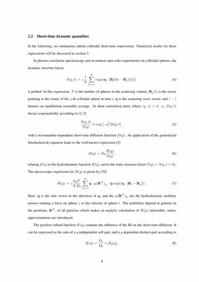
In photon correlation spectroscopy and in neutron spin echo experiments on colloidal spheres, the

dynamic structure factor,

S(q, t) = 〈 1N

N∑

l,j=1

exp{iq · [Rl(0)−Rj(t)]}〉 . (4)

is probed. In this expression, N is the number of spheres in the scattering volume, Rj(t) is the vector

pointing to the center of the j-th colloidal sphere at time t, q is the scattering wave vector, and 〈· · · 〉denotes an equilibrium ensemble average. At short correlation times where τB ¿ t ¿ τI , S(q, t)

decays exponentially according to [2, 3]

S(q, t)S(q)

≈ exp[−q2D(q) t

], (5)

with a wavenumber-dependent short-time diffusion function D(q). An application of the generalized

Smoluchowski equation leads to the well-known expression [3]

D(q) = D0H(q)S(q)

, (6)

relating D(q) to the hydrodynamic function H(q), and to the static structure factor S(q) = S(q, t = 0).

The microscopic expression for H(q) is given by [70]

H(q) = 〈 kBT

N D0

N∑

l,j=1

q · µ(RN )l j · q exp{iq · [Rl −Rj ]}〉 . (7)

Here, q is the unit vector in the direction of q, and the µ(RN )lj are the hydrodynamic mobility

tensors relating a force on sphere j to the velocity of sphere l. The mobilities depend in general on

the positions, RN , of all particles which makes an analytic calculation of H(q) intractable, unless

approximations are introduced.

The positive-valued function H(q) contains the influence of the HI on the short-time diffusion. It

can be expressed as the sum of a q-independent self-part, and a q-dependent distinct-part according to

H(q) =Ds

D0+ Hd(q) , (8)

9

where Ds is the short-time translational self-diffusion coefficient. The coefficient Ds gives the initial

slope of the particle mean squared displacement W (t), defined in three dimensions by

W (t) =16〈[R(t)−R(0)]2〉 . (9)

In the large-q limit, the distinct part vanishes and H(q) becomes equal to Ds/D0. Without HI, H(q)

is equal to one for all values of q. Any variation in its dependence on the scattering wave number is

thus a hallmark of the influence of HI. In the experiment, H(q) is determined by short-time dynamic

measurement of D(q) in combination with a static measurement of S(q) [15, 71]. In physical terms,

H(q) can be interpreted as the (reduced) short-time generalized mean sedimentation velocity in a

homogeneous suspension subject to weak force field collinear with q and oscillating spatially as cos(q·r). As a consequence,

limq→0

H(q) =Us

U0, (10)

is equal to the concentration-dependent short-time sedimentation velocity, Us(φ), of a slowly settling

suspension of spheres measured relative to the sedimentation velocity, U0, at infinite dilution. Thus

the long wavelength limit of H(q) can be determined in an alternative way by means of macroscopic

sedimentation experiments [72].

Furthermore, for qa ¿ 1, D(q) reduces to the short-time collective or gradient diffusion coeffi-

cient, Dc, given by

Dc =D0

S(0)Us

U0. (11)

The collective diffusion inherits its concentration dependence from Us(φ) and the thermodynamic

factor S(0) := limq→0 S(q). At non-zero concentration, Us(φ) < U0, and Dc(φ) is different from

D0. Likewise, Ds(φ > 0) is smaller than D0 in the presence of HI. Because of configurational changes

taking place for times t > τI , long-time transport properties are smaller than the short-time ones. A

case in point is self-diffusion, where the long-time coefficient Dl can be substantially smaller than Ds.

By contrast, sedimentation is hardly affected by dynamic caging so that the long-time sedimentation

velocity Ul in a fluid-like suspension is only slightly smaller than Us. The difference is less than 6%

even when a concentrated hard-sphere suspension is considered [73]. This is explained by the fact

that the equilibrium microstructure of identical spheres settling under a constant force is only slightly

perturbed by many-body HI, and not affected at all by the pairwise additive two-body part of the HI.

10

Up to this point only translational diffusion has been discussed. For optically anisotropic spheres,

characterized in their orientation by a unit vector u(t), rotational dynamics can be probed by exper-

imental techniques sensitive to their orientation [40, 74]. In a depolarized dynamic light scattering

measurement, e.g., the rotational self-dynamic correlation function [39],

Sr(t) = 〈P2 (u(t) · u(0))〉 , (12)

is probed, with P2 denoting the Legendre polynomial of second order. At short times, Sr(t) decays

exponentially according to

Sr(t) ≈ exp{−6Dr t} , (13)

where the short-time rotational self-diffusion coefficient Dr is the rotational analogue of Ds. At finite

colloid concentration, rotational diffusion is slowed by the HI so that Dr(φ) < Dr0. Here, Dr

0 =

kBT/(8πη0a3) is the rotational diffusion coefficient at infinite dilution.

Many attempts have been made in the past to identify generalized Stokes-Einstein (GSE) relations

between diffusional and viscoelastic suspension properties. These relations are of interest also from

an experimental point of view since, provided they are valid, rheological properties are probed more

easily and for smaller probe volumes using scattering techniques. Out of several GSE proposals, we

will explore the following three short-time relations, namely [52, 76]

Ds(φ) =kBT

6πη∞(φ)a, (14)

and [40, 77]

Dr(φ) =kBT

8πη∞(φ)a3, (15)

and [52, 77]

D(qm; φ) =kBT

6πη∞(φ)a, (16)

which relate the high-frequency limiting viscosity η∞ to Ds, Dr, and to the short-time diffusion func-

tion D(q), respectively, the latter evaluated at the wave number qm where S(q) and H(q) attain their

maximum. In what follows, we will refer to D(qm) as the (short-time) cage diffusion coefficient, since

2π/qm characterizes the radius of the next-neighbor shell of particles. The short-time viscosity η∞

reflects the bulk dissipation in a suspension subject to a high-frequency, low amplitude shear oscilla-

tion of circular frequency ω with (τI)−1 ¿ ω ¿ (τη)−1. We will expose these relations to a stringent

test using our ASD simulation data for η∞(φ), in combination with simulation results for Ds, Dr, and

H(qm).

11

2.3 Computational methods

The main tool for calculating the short-time quantities discussed previously will be accelerated Stoke-

sian dynamics simulations, using a code for Brownian particles developed by Banchio and Brady [13],

and extended by us to charged spheres interacting via the OMF pair potential of Eqs. (1) and (2). This

code enables us to simulate the short-time properties of a larger number of spheres, typically up to

1000 placed in a periodically replicated simulation box, which leads to an improved statistics. The

details of this simulation method have been explained in Ref. [13] and will not be repeated here. To

speed up the computation of short-time quantities such as H(q), which require for their computation

a single-time equilibrium averaging only, we have generated a set of equilibrium configurations using

a Monte-Carlo (MC) simulation code in the case of charge-stabilized spheres, and a Molecular Dy-

namics (MD) simulation code for neutral hard spheres. The many-body HI have been computed using

the ASD scheme. To correct for finite-size effects arising from the periodic boundary conditions, the

ASD simulations have been extrapolated to the thermodynamic limiting form of H(q) by using the

finite-size scaling correction

H(q) = HN (q) + 1.76S(q)η0

η∞(φ)(φ/N)1/3 , (17)

which, for q →∞, includes the finite-size correction for Ds as a special case. This correction formula

was initially proposed by Ladd in the framework of LB simulations of colloidal hard spheres [5,21,22].

The finite-size scaling form used to extrapolate to the H(q) of an infinite system requires thus to

compute the high-frequency limiting viscosity η∞(φ). Whereas empirical expressions for η∞(φ) are

available in the case of hard spheres (see the following subsection), simulations of η∞ are required in

general for charge-stabilized spheres. In section 3, we will show that the simulation data obtained for

various N collapse neatly on a single master curve once Eq. (17) has been used. The resulting master

curve is identified with the finite-size corrected form of H(q).

The only analytic method available to date allowing to predict the H(q) of dense suspensions of

neutral or charge-stabilized spheres, is the (zeroth order) renormalized density fluctuation expansion

method of Beenakker and Mazur [32]. This so-called δγ method is based on a partial resummation of

the many-body HI contributions. According to this scheme, H(q) is obtained to leading order in the

renormalized density fluctuations from [32, 45]

Hd(q) =32π

∫ ∞

0d(ak)

(sin(ak)

ak

)2

[1 + φSγ0(ak)]−1×∫ 1

−1dx

(1− x2

)[S(|q− k|)− 1] , (18)

12

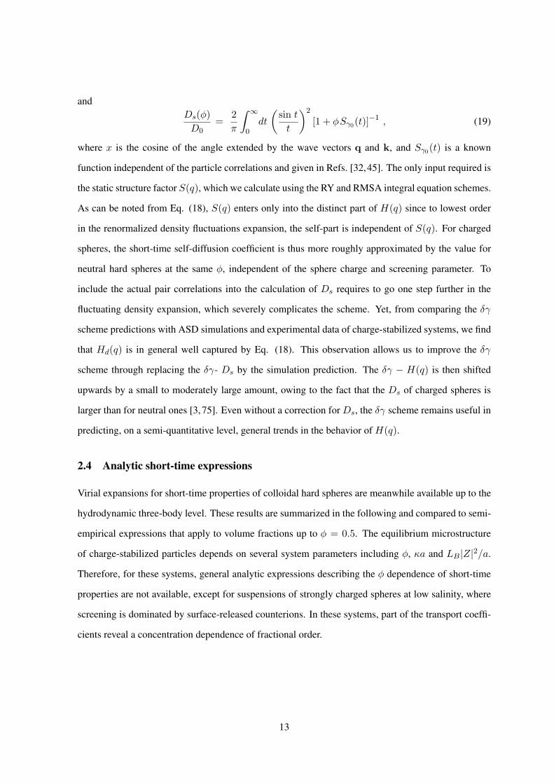
andDs(φ)

D0=

2π

∫ ∞

0dt

(sin t

t

)2

[1 + φSγ0(t)]−1 , (19)

where x is the cosine of the angle extended by the wave vectors q and k, and Sγ0(t) is a known

function independent of the particle correlations and given in Refs. [32,45]. The only input required is

the static structure factor S(q), which we calculate using the RY and RMSA integral equation schemes.

As can be noted from Eq. (18), S(q) enters only into the distinct part of H(q) since to lowest order

in the renormalized density fluctuations expansion, the self-part is independent of S(q). For charged

spheres, the short-time self-diffusion coefficient is thus more roughly approximated by the value for

neutral hard spheres at the same φ, independent of the sphere charge and screening parameter. To

include the actual pair correlations into the calculation of Ds requires to go one step further in the

fluctuating density expansion, which severely complicates the scheme. Yet, from comparing the δγ

scheme predictions with ASD simulations and experimental data of charge-stabilized systems, we find

that Hd(q) is in general well captured by Eq. (18). This observation allows us to improve the δγ

scheme through replacing the δγ- Ds by the simulation prediction. The δγ − H(q) is then shifted

upwards by a small to moderately large amount, owing to the fact that the Ds of charged spheres is

larger than for neutral ones [3,75]. Even without a correction for Ds, the δγ scheme remains useful in

predicting, on a semi-quantitative level, general trends in the behavior of H(q).

2.4 Analytic short-time expressions

Virial expansions for short-time properties of colloidal hard spheres are meanwhile available up to the

hydrodynamic three-body level. These results are summarized in the following and compared to semi-

empirical expressions that apply to volume fractions up to φ = 0.5. The equilibrium microstructure

of charge-stabilized particles depends on several system parameters including φ, κa and LB|Z|2/a.

Therefore, for these systems, general analytic expressions describing the φ dependence of short-time

properties are not available, except for suspensions of strongly charged spheres at low salinity, where

screening is dominated by surface-released counterions. In these systems, part of the transport coeffi-

cients reveal a concentration dependence of fractional order.

13

2.4.1 Hard spheres

The following truncated virial expansion results for hard spheres have been derived by Cichocki and

collaborators [35–37]

Ds/D0 = 1− 1.832φ− 0.219φ2 +O(φ3) (20)

Dr/Dr0 = 1− 0.631φ− 0.726φ2 +O(φ3) (21)

Us/U0 = 1− 6.546φ + 21.918φ2 +O(φ3) (22)

η∞/η0 = 1 + 2.5φ + 5.0023φ2 + 9.09φ3 +O(φ4) . (23)

These results fully account for HI up to the three-body level, and they include lubrication corrections.

The virial expression for η∞ contains a term proportional to φ3, since the viscosity is influenced by

particle correlations only when at least terms of quadratic order in φ are considered. From the virial

expressions for Ds and η∞, we note that the GSE expressions in Eqs. (14) and (15) are violated to a

certain extent to quadratic order in φ.

Eq. (22) for the sedimentation coefficient divided by the expansion, S(0) = 1 − 8φ + 34φ2 +

O(φ3), for the reduced osmotic compressibility of hard spheres, gives the 2nd-order virial result

Dc

D0= 1 + 1.454φ− 0.45 φ2 +O(φ3) (24)

for the collective diffusion coefficient valid up to quadratic order in φ. This expression describes a

weak initial increase in Dc when φ is increased. From the simulation results discussed in section 3) we

will see that this slow increase of Dc extends up to the concentration φ ≈ 0.5 where the system starts

to freeze. For charged spheres, the initial of Dc(φ) at small φ is typically far steeper. Moreover, on

further increasing φ, Dc passes through a maximum. This maximum is due to the competing influences

of Us and S(0). At small φ, S(0), decreases faster in φ than the sedimentation coefficient, whereas

this trend is reversed at larger φ [6, 45, 69] where the slowing influence of the HI becomes strong.

Although the OMF potential used in this simulation study is purely repulsive, a few comments on the

influence of attractive interactions are in order here. For particles subject to a significant short-range

attractive interaction part such as lysozyme globules [78], Dc(φ) can decrease with increasing φ and

attain values well below D0 [79]. Attractive forces tend to enlarge both the sedimentation velocity

and the compressibility, but the raise in the compressibility is larger and causes Dc to decrease with

increasing φ [79]. Attractive forces tend to increase the probability of neighboring particles to be

14

found at close proximity, causing thus a decrease in the short-time self-diffusion coefficient through

the stronger passive hindrance of the self-motion by neighboring particles [80]. This corresponds to

an attraction-induced increase in the high-frequency limiting viscosity [81].

A few semi-empirical expressions for short-time properties of hard spheres are frequently used in

the literature. Here we quote a formula for the self-diffusion coefficient proposed by Lionberger and

Russel [82]Ds

D0= (1− 1.56φ) (1− 0.27φ) . (25)

This expression conforms overall well, up to φ = 0.3, with the truncated virial expansion result for Ds

in Eq. (20), it reduces to the correct low-density limit 1− 1.83φ +O(φ2), and it diverges at the value

φrcp ≈ 0.64 where random close packing occurs. For volume fractions exceeding 0.3, the second order

virial expression for Ds ceases to be applicable [69].

The bulk of experimental data on η∞ conforms overall well with another empirical expression of

Lionberger and Russel [82],

η∞η0

=1 + 1.5φ

(1 + φ− 0.189φ2

)

1− φ (1 + φ− 0.189φ2). (26)

This formula has built in the exact Einstein limiting law at very small concentrations, and it diverges

for random close packing. The force multipole simulation data of η∞ obtained by Ladd are well fitted

by the formula [21]η∞η0

=1 + 1.5φ (1 + S(φ))1− φ (1 + S(φ))

, (27)

with S(φ) = φ + φ2 − 2.3φ3. In section 3 we will show that our ASD simulation data for the short-

time viscosity conform to the simulation results of Ladd, and that the third-order virial expression for

η∞ in Eq. (23) is applicable up to φ ≈ 0.25. Instead of showing a comparison with experimental data

for η∞, we will merely compare the simulation data to the outcome of Eq. (26), used as a representative

of the experimental data. For a Saito-like expression for η∞ based on two-body HI see [83].

The principal peak value, H(qm), of H(q) occurs practically at the same wave number, qm, where

S(q) attains its largest value. The peak height is well represented by the linear form [52],

H(qm) = 1− 1.35φ , (28)

which is valid for all concentrations up to the freezing concentration of hard spheres. This remarkable

expression should be compared to the prediction of the δγ scheme, with PY input for S(q), which is

15

well represented, for densities φ < 0.45, by the quadratic form [48]

H(qm) = 1− 2.03φ + 1.94φ2 . (29)

As we will show, the δγ scheme underestimates the correct peak height described by Eq. (28). For

φ < 0.35, H(qm) is moderately underestimated, but it is strongly overestimated for φ > 0.4.

On dividing Eq. (28) for H(qm) by an empirical expression for the peak height of the Verlet-Weiss

corrected PY-S(q), that is of good accuracy up to φ ≤ 0.5, namely by [84]

S(qm) = 1 + 0.644φ gCS(2a+) , (30)

where

gCS(2a+) =(1− 0.5φ)(1− φ)3

, (31)

we obtain an analytic expression for D(qm) which is in perfect agreement with experimental data

on hard spheres [85], LB simulations of Behrend [5], and with our ASD simulation results. This

expression for D(qm), can be used to scrutinize for hard spheres the validity of the GSE relation

(16) relating η∞ to D(qm). In Eq. (31), gCS(2a+) is the Carnahan-Starling contact value for the

radial distribution function of hard spheres which is found to be in good agreement with computer

simulations [66, 86]. According to Eq. (30), S(qm;φ = 0.494) = 2.85, in agreement with the

empirical Hansen-Verlet rule for the onset of freezing [66].

Simulation data for the collective diffusion coefficient, Dc(φ), are readily obtained from the force

multipole [21] and the LB simulation [5] data for Us/U0, on dividing these data through S(0) as

described by the rather accurate Carnahan-Starling expression,

SCS(0) =(1− φ)4

(1 + 2φ)2 + φ3(φ− 4). (32)

The so-obtained simulation data can be compared to the second order virial expression for Dc. This

comparison shows that the latter is applicable up to surprisingly large concentrations φ ≤ 0.4. At

larger values φ > 0.4, Dc is underestimated. Note here that S(0) calculated both in the CS and PY

approximations remains exact up to quadratic order in φ. For φ = 0.5, the Carnahan-Starling predicted

value for S(0) exceeds the PY value by only 12%.

2.4.2 Charge-stabilized spheres

In contrast to hard spheres, a regular virial expansion is not applicable to determine the diffusion

transport coefficient of strongly charged spheres in low salinity suspensions [3].

16

Instead, for de-ionized systems, the following non-linear concentration dependencies have been

predicted by theory [3, 46, 47, 87]

Ds/D0 = 1− at φ4/3 (33)

Dr/Dr0 = 1− ar φ2 (34)

Us/U0 = 1− as φ1/3 , (35)

with parameters at ≈ 2.5 and ar ≈ 1.3 which depend only weakly on the particle charge and size. The

coefficient as ≈ 1.8 in the expression for the sedimentation coefficient is nearly constant. The present

expressions for Dr and Ds have been confirmed experimentally [69, 75], and we will show that they

conform with existing LB and our ASD simulation data up to φ ≈ 0.35 and φ ≈ 0.1, respectively.

The peak height of H(q) in these systems is well approximated, for densities φ ≤ 10−2, by the

non-linear form [52]

H(qm) ≈ 1 + pm φ0.4 . (36)

The coefficient pm > 0 in this expression is moderately depending on Z and κa. It is larger for more

strongly structured suspensions characterized by a higher peak in S(q). The exponent 0.4, however, is

independent of the system parameters, as long as the particle charge is large enough that the physical

hard core of the spheres remains totally masked by a sufficiently strong and long-range electrostatic

repulsion. The values of the exponents in the short-time expressions of Eqs. (33-36) can be attributed

essentially to the fact that, in de-ionized suspensions of strongly charge spheres, the location, rm =

2π/qm, characterizing the location of the principal peak in g(r) that characterizes the location of the

next-neighbor shell coincides, within 5% of accuracy (see [87] and Fig. 5), with the geometric mean

distance r = n−1/3 = a(4π/3φ)1/3 of two spheres.

To calculate H(q) for very dilute de-ionized suspensions, it suffices to account for the leading-

order far-field form of the hydrodynamic mobilities only, which amounts to the neglect of hydrody-

namic reflections with constant force densities on the sphere surfaces (so-called Rotne-Prager approx-

imation of the HI). Then a simple analytic expression is obtained [3, 88],

HRP(y) = 1− 15φj1(y)

y+ 18φ

∫ ∞

1dxx [g(x)− 1]

(j0(xy)− j1(xy)

xy+

j2(xy)6x2

), (37)

where y = 2qa, x = r/(2a), and jn is the spherical Bessel function of order n. Experimental results

for the hydrodynamic functions of highly dilute dispersions of strongly charged particles are well de-

scribed by this expression [90]. However, Eq. (37) necessarily fails for larger particle densities, when

17

near-field HI contributions come into play [3]. It is then necessary to resort to δγ scheme calcula-

tions or to simulations of H(q). In Rotne-Prager (RP) approximation, the short-time sedimentation

coefficient is given by,

Us/U0 = 1 + φ + 12φ

∫ ∞

0dxxh(x) = 1 + φ + 12φH(z → 0) , (38)

where H(z) is the Laplace transform of x h(x) and h(x) = g(x) − 1. Using the analytic Percus-

Yevick expression for the function H(z) of hard spheres given by Wertheim [91], the RP sedimentation

coefficient is

Us/U0 =(1− φ)3

1 + 2φ+

15

φ2 ≈ 1− 5φ +665

φ2 +O(φ3) , (39)

where we have accounted for the extra term φ2/5 omitted by Brady and Durlofsky [33] in their orig-

inal derivation of Us in RP approximation. At large values of φ, this correction term spoils to some

extent the reasonably good agreement with the simulation data of hard spheres, that would be observed

otherwise (see subsection 3.4). On first sight one might expect the RP approximation to be very poor

for hard spheres. With regard to sedimentation, however, it actually captures the main effect since,

as discussed thoroughly by Brady and co-workers [16, 17, 33], the contribution of near-field HI to the

sedimentation velocity, in the form of induced stresslets which are of O(r−4) and lubrication is quite

small, unless φ is so large that near-contact configurations become non-negligible.

The short-time viscosity in dilute suspensions of strongly repelling spheres with prevailing two-

body HI can be computed from [1, 89]

η∞η0

= 1 +52φ (1 + φ) +

152

φ2

∫ ∞

2dxx2 g(x)J(x) , (40)

where the rapidly and monotonically decaying function J(x) accounts for two-body HI. It is known

numerically, and as an expansion in a/r, with long-distance asymptotic form J(x) = (15/2)x−6 +

O(x−8), for x defined here and in the following as x = r/a À 1. The (5/2) φ2 term arises from

regularizing the integral, which is a summation over induced hydrodynamic force dipoles. The integral

involving the radial distribution function is at most of order one. In dilute and deionized systems, where

rm ∼ φ−1/3, the integral is a small quantity of O(φ). For these systems, η∞ is well approximated by

the single-body part in Eq. (40). If we account in Eq. (40) for the leading-order long-distance part of

J(x) only, thenη∞η0

≈ 1 +52φ (1 + φ) +

75256

φ2

∫ ∞

0duu4 G(u) , (41)

18

where G(u) is the Laplace transform of x g(x). This expression is handy to use, since the RMSA

provides an analytic expression for G(u). Next, we schematically approximate g(x) in Eq. (40) by the

form [52]

g(x) ≈ (r/a)A(φeff)δ(x− r/a) + Θ(x− r/a) , (42)

consisting of a step function describing the correlation hole formed around each sphere, and a delta-

distribution term describing the first maximum in g(r). To determine the amplitude factor A(φeff),

with φeff = φ(r/a)3 = π/6, we use the compressibility equation

1 + 3φeff

∫ ∞

0dxx2 [g(x)− 1] = χT (φeff) , (43)

where χT (φeff) = kBT (∂n/∂p)T is the reduced isothermal compressibility of hard spheres, evaluated

at φeff, for which we employ the Carnahan-Starling equation of state. As a result, we obtain A(φeff) ≈0.25, which follows also from neglecting the very small χT of deionized systems as compared to one.

Using this value for A leads to [52]

η∞η0

≈ 1 +52φ (1 + φ) + 7.9φ3 , (44)

which includes a positive-valued correction term, 7.9 φ3, with a coefficient that is smaller than the

coefficient, 9.09, of the third-order density contribution in the virial expansion of hard spheres in Eq.

(23). The correction term describes the viscosity contribution arising from binary particle correlations,

and we emphasize that it is of cubic order in φ since r ∼ φ−1/3 and J(x) ∼ 1/x6 in deionized systems.

As we will show, Eq. (44) is in good accord with our ASD simulation data on deionized suspensions,

for the concentration range considered (see subsection 3.3).

3 RESULTS AND DISCUSSION

The ASD simulation and δγ theory results for the colloidal short-time properties of charge-stabilized

spheres shown is this section are based on the one-component macroion fluid model (OMF), with the

effective pair potential given by Eqs. 1 and 2. This model contains neutral hard spheres as the limiting

case of zero colloid charge or infinitely strong screening. The solvent is described as a structureless

continuum of dielectric constant ε = 10 and temperature T = 298.15 K (25 o C), with a Bjerrum length

of LB = 5.617 nm. The colloidal sphere radius is selected as a = 100 nm, and the effective colloid

charge number is Z = 100, corresponding to LB|Z|/a = 5.62 and a low-salt contact potential of

19

βu(2a+) = 281 valid for κa ¿ 1. Most of our simulation and theoretical results on charge-stabilized

systems discussed in the following have been obtained using these interaction parameters, and it will

be noted explicitly if other system parameters have been used. The selected system parameters are

representative of suspensions of strongly charged colloidal spheres. We focus our discussion on de-

ionized charge-stabilized suspensions, where all excess electrolyte ions have been removed, and on

suspensions of neutral colloidal spheres. However, for a selected number of properties we will also

discuss the transition from salt-free to neutral hard-sphere suspensions as the salt content is increased.

The short-time properties of systems with finite amount of added salt are bounded by the values for

these two limiting model systems, as we will illustrate by examples. All short-time properties are

explored over an extended range of volume fractions where the suspensions show fluid-like order.

3.1 Static structure factor

In Fig. 1, we discuss the q-dependence of the static structure factor of hard spheres, for three selected

volume fractions as indicated in the figure. The RY predictions of S(q) are nearly coincident with the

MD simulation results, and with the Verlet-Weiss corrected PY structure factor, even for the largest

volume fraction considered. The uncorrected PY approximation, however, noticeably overestimates

the structure factor peak height, S(qm), for concentrations larger than φ = 0.4. This can be clearly

seen from Fig. 2, which shows the PY-S(qm) in comparison with the accurate VW-PY peak height

that is well parameterized by the analytic expression in Eq. (30). Fig. 3 displays the corresponding

hard-sphere radial distribution functions g(r). The RY scheme is in better agreement with the MD

simulation results than the PY approximation. However, it also underestimates the contact value of

g(r) for volume fractions near the freezing transition value. The Verlet-Weiss corrected PY scheme,

on the other hand, has been designed to agree well with the simulation data.

The static structure factor of a salt-free suspension of highly charged spheres is shown in Fig. 4 for

volume fractions as indicated. The RY-calculated S(q), obtained using the same system parameters as

in the simulation, nearly coincides with the simulation data over the whole displayed range of wave

numbers. Small differences are observed in S(qm) only, which at larger φ is slightly underestimated

by the RY scheme. The agreement between RY theory and simulation in the peak height becomes

even better for systems with added electrolyte. In the figure, we do not show the S(q) obtained from

the linear RMSA scheme. This scheme requires usually somewhat larger values of the effective col-

20

0 2 4 6qa

0

0.5

1

1.5

2

2.5

3

S(q)

PYRYPY-VWMD

φ = 0.49

φ = 0.40

φ = 0.20

Figure 1: (Color online) Static structure factor of a hard-sphere suspension at various volume fractions φ as

indicated. Comparison between MD simulation data and Rogers-Young (RY), Percus-Yevick (PY) and Verlet-

Weiss corrected Percus-Yevick (PY-VW) integral equation schemes.

0 0.1 0.2 0.3 0.4 0.5φ

1

1.5

2

2.5

3

3.5

4

S(q m

)

PYVW-fitMD

Figure 2: (Color online) Peak value, S(qm), of the hard-sphere static structure factor. MD simulation data

(symbols) are compared with PY calculations and the PY-VW fitting formula in Eq. (30).

21

2 3 4 5r/a

0

1

2

3

4

5

6

g(r)

PY-VWRYPYMD

φ = 0.49

φ = 0.40

φ = 0.20

Figure 3: (Color online) Hard-sphere radial distribution function corresponding to Fig. 1. The curves for

φ = 0.40 and 0.20 are shifted to the right by a and 2a, respectively.

loid charge, Ze, to match the peak height of the simulated S(q). This reflects the well-known fact

that in RMSA the pair correlations are somewhat underestimated for suspensions of strongly charged

particles. However, once the RMSA effective charge has been adjusted accordingly, remarkably good

agreement is observed between the RMSA and RY structure factors [6]. Moreover, even for a non-

adjusted effective charge, the position, qm, of the structure factor peak is very well described by the

RMSA scheme. The position, rm, of the principal peak in the radial distribution function in these

systems coincides within 5 % with the average geometric distance, r = n−1/3, of two particles [87],

which is here the only physically relevant static length scale. This feature has been used to derive

the concentration-scaling predictions quoted in Eqs. (33-36) and (44). That the peak position, qm,

for these systems scales indeed as 2π/r =(6π2φ

)1/3/a, up to a factor of about 1.1, can be seen

from Fig. 5 which displays the RMSA prediction for qm, in comparison with the VW-PY calculated

peak position of hard spheres. The two curves tend to converge at large φ since rm approaches 2a for

increasing concentration. The red circles describe a system at φ = 0.15, where ns is increasing from

1× 10−6 to 1× 10−4M (i.e., from κa = 2 to 10). This illustrates the transition, for a fixed φ, from a

low-salt to a hard-sphere-like system.

22

0 1 2 3 4

qa

0

0.5

1

1.5

2

2.5

3

S(q)

φ = 0.0001φ = 0.005φ = 0.055φ = 0.105RY

Figure 4: (Color online) Static structure factor of a de-ionized charge-stabilized suspension at volume fractions

as indicated. The MC simulation data (symbols) are compared with Rogers-Young calculations (solid lines)

using identical system parameters, i.e., Z = 100, LB = 5.62 nm and ns = 0.

0.0001 0.001 0.01 0.1 1φ

0.1

1

q m a

PY-VW (hard spheres)RMSA (deionized system)

1.095 * 2π [3φ/(4π)]1/3

Figure 5: (Color online) Concentration dependence of the peak position, qm, of the static structure factor of

de-ionized suspension in units of the particle radius. The green diamonds are the RMSA result for ns = 0. Blue

circles: MC data for ns = 0; Black circles: MC result for a collection of systems with varying amount of added

salt. Red circles: MD data for a system at φ = 0.15 with ns varying from 1×10−6 to 1×10−4 M. Additionally

shown is the peak-position wave number of hard spheres, as predicted by the Verlet-Weiss corrected PY scheme.

23

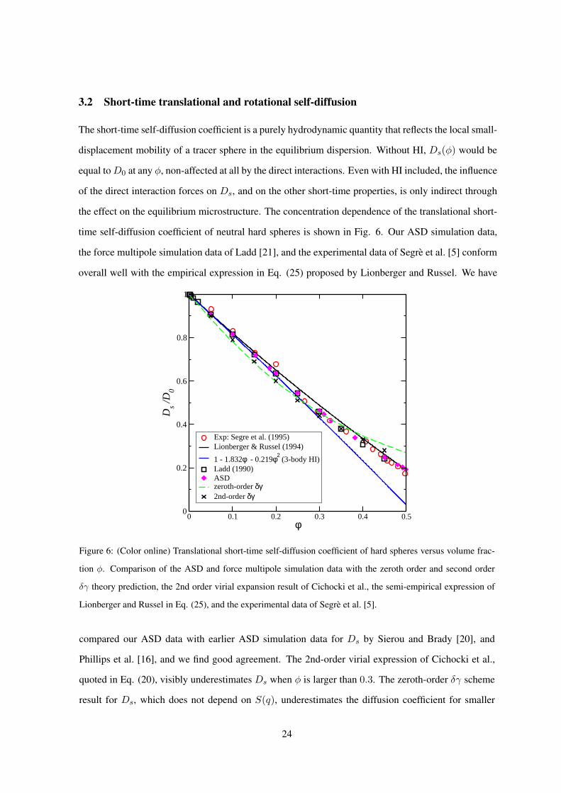
3.2 Short-time translational and rotational self-diffusion

The short-time self-diffusion coefficient is a purely hydrodynamic quantity that reflects the local small-

displacement mobility of a tracer sphere in the equilibrium dispersion. Without HI, Ds(φ) would be

equal to D0 at any φ, non-affected at all by the direct interactions. Even with HI included, the influence

of the direct interaction forces on Ds, and on the other short-time properties, is only indirect through

the effect on the equilibrium microstructure. The concentration dependence of the translational short-

time self-diffusion coefficient of neutral hard spheres is shown in Fig. 6. Our ASD simulation data,

the force multipole simulation data of Ladd [21], and the experimental data of Segre et al. [5] conform

overall well with the empirical expression in Eq. (25) proposed by Lionberger and Russel. We have

0 0.1 0.2 0.3 0.4 0.5φ

0

0.2

0.4

0.6

0.8

1

Ds /D

0

Exp: Segre et al. (1995)Lionberger & Russel (1994)

1 - 1.832φ - 0.219φ2(3-body HI)

Ladd (1990)ASDzeroth-order δγ2nd-order δγ

Figure 6: (Color online) Translational short-time self-diffusion coefficient of hard spheres versus volume frac-

tion φ. Comparison of the ASD and force multipole simulation data with the zeroth order and second order

δγ theory prediction, the 2nd order virial expansion result of Cichocki et al., the semi-empirical expression of

Lionberger and Russel in Eq. (25), and the experimental data of Segre et al. [5].

compared our ASD data with earlier ASD simulation data for Ds by Sierou and Brady [20], and

Phillips et al. [16], and we find good agreement. The 2nd-order virial expression of Cichocki et al.,

quoted in Eq. (20), visibly underestimates Ds when φ is larger than 0.3. The zeroth-order δγ scheme

result for Ds, which does not depend on S(q), underestimates the diffusion coefficient for smaller

24

values of φ, whereas Ds is overestimated for φ exceeding 0.4. Beenakker and Mazur have determined

2nd order correction terms for Ds based on the PY input for S(q) (see Fig. 7, and table III in [32]).

These corrections improve the agreement of the δγ scheme with the simulation data for φ > 0.3.

In Fig. 7, we compare the concentration dependence of the Ds for charged spheres in a de-ionized

0.001 0.01 0.1φ

0.2

0.4

0.6

0.8

1

Ds /D

0

HS: Lionberger & Russel (1994)

CS: 1 - 2.5 φ4/3

Figure 7: (Color online) Translational short-time self-diffusion coefficient of charged spheres in a salt-free

suspension (labelled by CS) versus the hard-sphere result (HS). The symbols are our ASD simulation results.

Green diamonds: hard spheres; blue circles: de-ionized suspension; red circles: transition from a de-ionized

system, at φ = 0.15, to a hard-sphere-like system on increasing ns from 1× 10−6 to 1× 10−4 M; black circles:

collection of systems with varying amount of added salt.

suspension with that of neutral hard spheres. The symbols denote our ASD simulation data. For

all volume fractions considered, the simulation data of the de-ionized systems which are of fluid-

like order conform well with the fractional concentration-scaling in Eq. (33), for a parameter value

at = 2.5. The φ4/3-dependence of Ds has been experimentally confirmed in recent dynamic light

scattering experiments on charge-stabilized suspensions treated by an ion exchange resin to remove

residual salt ions [75]. The hydrodynamic self-mobility function which enters into the expression for

Ds is rather short-ranged, with a long-distance asymptotic form proportional to r−4. Therefore, Ds

increases with decreasing ionic strength (i.e., decreasing κ), since the hydrodynamic slowing is weaker

25

for charged spheres that repel each other over longer distances. As can be noticed from the red symbols

representing a system at φ = 0.15 with various amounts of added salt, the addition of salt reduces Ds

towards the lower boundary set by the hard-sphere value reached in the limit of strong electrostatic

screening. This generic salt-dependence of Ds in our calculations conforms with experimental results

obtained for charge-stabilized suspensions [76, 92]. The ASD results for Ds in all explored systems

are located in between the two limiting curves for zero added salt and neutral hard spheres (see, e.g.,

the black circles representing a collection of very different systems with varying salt content).

0 0.1 0.2 0.3 0.4 0.5 0.6φ

0.3

0.4

0.5

0.6

0.7

0.8

0.9

1

Dr /D

0r

DDLS: Degiorgio et al. (1995)

ASDLB-Simulation: Hagen et al. (1999)

1 - 0.63 φ − 0.73 φ2(3-body HI)

Figure 8: (Color online) Short-time rotational self-diffusion coefficient of hard spheres versus volume fraction.

The symbols are our ASD results and correspond to the ones in Figs. 6 and 7. The ASD data are compared

with Lattice-Boltzmann simulation data of Hagen et al. [25], the truncated virial expansion (in Eq. (21)), and

the experimental data of Degiorgio et al. [74]. The 2nd-order virial expression remains valid up to φ = 0.45.

Our ASD simulation results for the short-time rotational self-diffusion coefficient of hard spheres

are depicted in Fig. 8, and compared with earlier LB simulation data of Hagen et al., depolarized

dynamic light scattering data of Degiorgio et al., and the 2nd-order virial form in Eq. (21) derived by

Cichocki and coworkers [35]. We have checked our ASD data for the hard-sphere Dr against earlier

SD simulation data of Phillips et al. [16] and find good agreement. The 2nd-order virial form remains

26

valid up to remarkably large volume fractions that extend to the freezing transition concentration. This

suggests that all higher-order virial coefficients in Ds are small or mutually cancel each other. In

determining short-time properties such as Ds, Dr and η∞, only small distance changes are probed that

amount typically to a small fraction of the particle diameter. Therefore, short-time quantities are rather

insensitive to qualitative changes in the microstructure, and cross over smoothly into the liquid-solid

coexistence regime. This should be contrasted to long-time dynamic properties, which may change

drastically in their behavior at equilibrium and non-equilibrium transition points.

0.001 0.01 0.1φ

0.8

0.85

0.9

0.95

1

Dr /D

0r

HS: 1 − 0.631 φ − 0.726 φ2

CS: 1 − 1.3 φ2

Figure 9: (Color online) Short-time rotational self-diffusion coefficient of a de-ionized suspension of charged

spheres (CS), in comparison to the Dr of neutral spheres (HS). The symbols are our ASD simulation results,

with same symbols and color coding as in Fig. 7. The quadratic scaling form in Eq. (34), which accounts for

far-field 3-body HI corrections, remains valid up to remarkably large φ. The Dr for systems with added salt is

bounded from above and below, respectively, by the two limiting curves describing de-ionized charged-sphere

and neutral hard-sphere systems.

Our ASD simulation data (symbols) for the short-time rotational diffusion coefficient of charge-

stabilized and neutral colloidal spheres are shown in Fig. 9. The quadratic scaling form in Eq. (34),

valid for deionized systems and accounting for far-field 3-body HI, is seen to apply up to remarkably

27

large values of φ. It should be stressed here that Eq. (34) is not the result of a standard virial expansion,

since for zero added salt the system is dilute only regarding the hydrodynamic interactions, which can

be described thus on the two-body and leading-order three-body level, but non-dilute regarding direct

interactions. The radial distribution function in these systems has pronounced oscillations typical for

strong fluid-like ordering. The scaling prediction in Eq. (34) has been confirmed additionally by LB

simulations of Hagen et al. [25], which show that it applies accurately up to φ ≈ 0.3. The coefficient

Dr of charge-stabilized suspensions decreases with increasing amount of added salt ions, for the same

reason as discussed earlier in the context of Ds. For short-time rotational diffusion, the hydrodynamic

self-mobility tensor associated with Dr decays asymptotically as r−6, i.e., by two powers in r stronger

than the hydrodynamic mobility related to translational self-diffusion. This is the reason why Dr is

quite sensitive to the ionic strength, so that a small residual amount of excess ions leads to a curve for

Dr located below the upper limiting curve described by Eq. (34). The pronounced sensitivity of Dr

on the ionic strength has been observed also experimentally [40]. For larger amounts of added salt, the

lower limiting curve for Dr describing neutral hard spheres is reached (see red symbols in Fig. 9).

3.3 High-frequency limiting viscosity

We discuss next the high-frequency limiting suspension viscosity measured by high-frequency and

low-amplitude shear oscillation rheometers in the Newtonian regime where shear-thinning is absent.

Under these conditions, the equilibrium microstructure remains unaffected by the imposed shear flow.

Computer simulation and theoretical results for the η∞ of colloidal hard spheres are displayed in Fig.

10. The expression in Eq. (27) given by Ladd, which fits his simulation data obtained up to φ = 0.45

(see table IV in [21]), is seen to apply to even larger values of φ where it conforms also with our

ASD simulation data, and the ones of Sierou and Brady [20]. There is a wealth of experimental

data available for η∞ with show a significant stray due to statistical errors and size polydispersity.

Instead of including experimentala data, we refer to the Lionberger-Russel formula in Eq. (26) as

an representative for the average of these data. The empirical Lionberger-Russel form for η∞ agrees

overall well with the simulation data. The 3rd-order virial expansion result in Eq. (23) is applicable

up to φ > 0.3. At larger φ, the uprise in η∞ is underestimated. The 2nd-order δγ theory result

for η∞, which has been calculated by Beenakker using the PY-S(q) as input, agrees overall well

with the ASD simulation data in the full concentration range up to φ ≈ 0.45 where it is applicable.

28

This is remarkable since the δγ theory accounts only approximately for near-field HI and disregards

lubrication. Moreover, in Fig. 10 we show the result for η∞ described by the modified Saito expression

η∞η0

= 1 +52

φ1 + 1.0009φ + 0.63Φ2

1− φ− 1.0009φ2 − 0.63Φ3, (45)

which has been derived by Cichocki et al. using their third-order virial expression result for the short-

time viscosity [37]. This expression strongly overestimates η∞ when φ exceeds 0.4. Out of the present

comparison of analytic viscosity expressions, Eq. (27) emerges as a handy formula which describes

the overall φ-dependence of η∞ very well. Our ASD simulation data for the η∞ of a de-ionized

0 0.1 0.2 0.3 0.4 0.5φ

0

5

10

15

η ∞/η

0

modified Saito expr.

Lionberger & Russel

3d. order virial: 1 + 2.5φ+ 5.0023φ2+ 9.09φ3

simulation fit: LaddASDLadd simulation data2nd. order δγ

Figure 10: (Color online) High-frequency limiting viscosity, η∞, of colloidal hard spheres versus φ. Displayed

are our ASD simulation data in comparison with the force multipole simulation data of Ladd [21], the third-order

truncated virial expansion result in Eq. (23), the semi-empirical Lionberger-Russel expression in Eq. (26), the

simulation fitting formula of Ladd in Eq. (27), the modified Saito expression of Cichocki et al. in Eq. (45), and

the 2nd order δγ-PY result taken from [43].

charge-stabilized suspension are shown in Fig. 11, and compared with the analytic expression in

Eq. (44) based on a schematic model calculation. This expression conforms with the simulation

data overall quite well for the liquid-state volume fractions considered (note that S(qm) ≈ 2.8 at

φ = 0.15). At smaller φ < 0.1, the first-order Einstein term part in Eq. (44) dominates. Furthermore,

we display the result for η∞ described in Eq. (40) which fully accounts of 2-body HI and is based on

the RMSA input for g(r). This result fully conforms with Eq. (44) in the whole φ-range considered.

29

The modest increase of η∞ with increasing volume fraction, and its very weak dependence on the

ionic strength noticed from ASD simulations for varying ns (not shown here) are features consistent

with the experimental findings of Bergenholtz et al. [76]. In fact, as can be noticed in the inset of

Fig. 11 where ASD viscosity data for hard spheres are compared with those of two deionized system,

the differences in the viscosities are quite small. The differences are largest at intermediate volume

fractions where two-body HI prevail. They become smaller at larger φ where the particles are close to

each other and near-field many-body HI is strong. The curves for η∞(φ) in systems with added salt are

1e-05 0.0001 0.001 0.01 0.1φ1

1.5

2

2.5

3

η ∞/η

0

ASDFull 2-body HI calculation

1 + 2.5φ + 2.5φ2

1 + 2.5φ + 2.5φ2 + 7.9 φ3

HS: Ladd fit formulaHS: ASD

0.01 0.1

0.001

0.01

0.1

1

η ∞/η

0 − 1

− 2

.5 φ

Figure 11: (Color online) High-frequency limiting viscosity of two de-ionized suspensions of charged spheres

(Circles: Z = 100, a = 100 nm, LB = 5.62 nm, ns = 0; diamonds: Z = 70, a = 25 nm, LB = 0.71 nm,

ns = 0 ). The ASD simulation data are overall well described by Eq. (44) which derives from a schematic

model for g(r) using the leading-order far-field HI contribution. For an expanded view of the differences, the

inset shows the excess short-time viscosity.

all located in between the two limiting curves for zero and infinite amount of added salt. Consistent

with a corresponding behavior of Ds(φ), the η∞ of a dilute charge-stabilized suspension is smaller than

that of a hard-sphere system at the same φ (compare Eq. (23) with Eq. (44)), reflecting the weaker

30

hydrodynamic dissipation of in charged-sphere systems due to the depletion of neighboring spheres

near contact caused by electrostatic repulsion. The experimental data in [76] and [92] conform with

the theoretically predicted trends even at large values of φ. At very large volume fractions, however,

many-body near-field HI come into play even in low-salt systems. Then, a hard-sphere-like behavior

of η∞ is approached, and Eqs. (40) and (44) do not apply any more (see the inset in Fig. 11).

3.4 Short-time sedimentation coefficient

We notice from comparing Eq. (22) with (35), that there is a remarkable difference at lower φ in the

concentration dependence of the short-time sedimentation velocity, Us, between hard spheres and de-

ionized charged-sphere systems. Results for the sedimentation coefficient of hard spheres obtained by

various methods are included in Fig. 12. As discussed earlier, near-field HI only have a small influence

on the sedimentation coefficient. This is the reason why the long-time sedimentation coefficient is only

slightly smaller than the short-time one, and why the δγ theory result, with its approximate account of

near-field HI without lubrication correction, agrees decently well with the force multipoles simulation

result of Ladd [21], and the LB simulation result of Segre et al. [5]. The LB data shown in the

figure have been obtained from multiplying the LB data for DC/D0 in [5] with SCS(0). The Rotne-

Prager approximation for Us given in Eq. (39) overestimates the simulated sedimentation velocity,

with growing difference for increasing concentration. Yet, the Rotne-Prager Us compares reasonably

well overall with the simulation data for small to intermediate values of φ, which reflects the weak

near-field HI dependence of Us for volume fractions which are not very large. The 2nd-order virial

result in Eq. (22) for Us is valid for φ ≤ 0.1 only, as signalled by the sign change in going from the

first to the second virial coefficient. Whereas the sedimentation velocity is little affected by memory

effects for reasons discussed already before, the zero-shear static viscosity, η(φ), and the long-time

self-diffusion coefficient, Dl(φ), differ substantially from their short-time counterparts. At long times,

direct forces influence the transport coefficients directly through a perturbation of the equilibrium

microstructure caused by the motion of a tagged sphere in the case of self-diffusion, and the shear

flow distortion in the case of the viscosity. To illustrate the pronounced difference between short-and

long-time viscosities, in Fig. 13 we have also included the result for η0/η∞ according to Eq. (27), and

the inverse of the static viscosity η0/η as predicted by the hydrodynamically rescaled mode-coupling

scheme (MCS). The latter compares well with experimental viscosity data on hard spheres [52]. For a

31

0 0.1 0.2 0.3 0.4 0.5

φ

0

0.2

0.4

0.6

0.8

1

Us/U

0

Simulation Ladd (1990)

δγ - theory

(1-φ)³/(1+2φ) + φ²/5

1 - 6.546φ + 21.918φ²

η0/η∞ (Eq. (27))

η0/η(φ) : HI-rescaled MCT

Simulation Segre et al. (1995)

Figure 12: (Color online) Short-time sedimentation coefficient, Us/U0, of a homogeneous hard-sphere suspen-

sion. The 2nd-order virial and Rotne-Prager approximation results, and the zeroth-order δγ scheme prediction

are compared with the accurate computer simulation results of Ladd [21], and LB simulations of Segre et al. [5].

Note here the strong difference between η0/η∞(φ) and η0/η(φ).

32

discussion of the static viscosity of colloidal hard spheres see also [18, 93]. In linear response theory,

the self-diffusion coefficient is obtained by considering a weak external force applied to a single tagged

sphere. For hard spheres, the influence of surrounding neutrally buoyant spheres can be then described

approximately by the high-frequency (in case of Ds) or the static viscosity (in case of Dl), giving

rise to the approximate validity of a generalized Stokes-Einstein relation between the self-diffusion

coefficient and the viscosity (see subsection 3.7 for a discussion of this relation). It is apparent from

Fig. 13 that such a simple mean-field-type picture is not valid in the case of sedimentation, since it

would imply that Us/U0 ≈ η0/η∞.

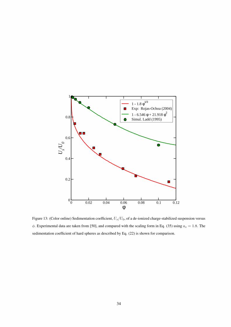
Recent experimental data for the sedimentation coefficient of a de-ionized charge-stabilized sus-

pension, obtained from a small-q scattering experiment [50], are shown in Fig. 13. These data are in

good agreement with Eq. (35) for as = 1.8, whose validity is a consequence of the dominating far-field

2-body HI, and the scaling relation r ∼ φ−1/3 obeyed in low-salinity systems for φ ≤ 0.1 [87]. That

charged spheres sediment more slowly than neutral ones can be rationalized as follows: For charged

spheres at low salinity, near-contact configurations are very unlikely due to the strong electric repul-

sion. On the average, this causes an enlarged laminar friction between the backflowing solvent part

which has its origin in the non-zero total force on the spheres, and the solvent layers adjacent to the

sedimenting spheres which are dragged along. Hasimoto [94] and Saffman [95] have shown that a

simple cubic lattice of widely separated spheres sediment with a velocity in accord with Eq. (13), but

for a slightly smaller parameter of as = 1.76. For the scaling relation in Eq. (35) to be valid, however,

a long-range periodicity of the particle configuration is not necessary. What is required only is a strong

and long-range inter-particle repulsion, which creates around each sphere a well-developed shell of

next neighbors of radius scaling as n−1/3.

3.5 Collective diffusion coefficient

On dividing Us/U0 by S(0), the short-time collective diffusion coefficient, Dc/D0, is obtained. This

coefficient can be measured in a low-q dynamic scattering experiment or, alternatively, in a macro-

scopic gradient diffusion experiment on ignoring in the latter case the small difference between long-

time and short-time collective diffusion. The simulation results of Ladd [21] and Segre et al. [5] for

hard spheres show a weak concentration dependence of Dc (see Fig. 14), which reflects very similar

φ-dependencies of Us and S(0). Up to φ = 0.4, the simulation data follow closely the 2nd-order virial

33

0 0.02 0.04 0.06 0.08 0.1 0.12φ

0

0.2

0.4

0.6

0.8

1

Us/U

0

1 - 1.8 φ1/3

Exp: Rojas-Ochoa (2004)

1 - 6.546 φ + 21.918 φ2

Simul. Ladd (1995)

Figure 13: (Color online) Sedimentation coefficient, Us/U0, of a de-ionized charge-stabilized suspension versus

φ. Experimental data are taken from [50], and compared with the scaling form in Eq. (35) using as = 1.8. The

sedimentation coefficient of hard spheres as described by Eq. (22) is shown for comparison.

34

result in Eq. (24) for Dc which, unlike to Us, points to a strong mutual cancellation of higher-order

virial contributions in the case of Dc. The δγ result for Dc shown in Fig. 14 has been obtained from

dividing the δγ-Us/U0 depicted in Fig. 12 through SCS(0). The underestimation of Dc at small φ,

0 0.1 0.2 0.3 0.4 0.5φ

1

1.5

2

2.5

3

Dc/D

0

δγ theory

1 + 1.454 φ − 0.45 φ2

Ladd-(Us/U

0)/S

CS(0)

Exp.: Segre et al. (1995)

Simulations: Segre et al. (1995)

Figure 14: (Color online) Short-time collective diffusion coefficient, Dc = D(q → 0), of hard spheres. Com-

parison between the simulation data of Ladd [21], obtained from dividing the simulated Us/U0 by SCS(0), LB

simulation data and dynamic light scattering data of Segre et al. [5], zeroth-order δγ theory prediction, and the

2nd-order virial result in Eq. (24).

and its gross overestimation for φ > 0.4, reflects a corresponding behavior in the δγ result for Us,

but is here more visible due to the division by SCS(0). We note here that the δγ result for Us remains

practically unchanged when, in place of the PY S(q), the Verlet-Weiss corrected structure factor is

used [44]. Significant deviations between experimental and simulation data are visible even at smaller

concentrations where the 2nd-order virial expansion applies. As noted in [5], these deviations might

result from the lack of experimental data at low enough wavenumbers to provide reliable extrapolations

to q = 0.

In charge-stabilized suspensions, Dc increases more rapidly with concentration and typically passes

35

through a distinct maximum which increases (decreases) and shifts to larger (smaller) values of φ for

growing particle charge (salt content). The observed maximum arises since, at larger φ, the hydrody-

namic hindrance determined by Us overcompensates the small osmotic compressibility proportional

to S(0). For recent δγ theory calculations of the Dc for charge-stabilized systems describing experi-

mental results for globular charged proteins, we refer to [6].

3.6 Hydrodynamic and short-time diffusion functions

Our ASD simulation results for the wave-number dependent hydrodynamic function H(q) have been

obtained using the finite-size correction scheme in Eq. (17), initially used for hard-sphere suspensions

[21, 22]. We have verified that this scheme gives a unique master curve also for charged spheres, over

the whole explored range of system sizes N , volume fractions, salt contents and effective charges. Fig.

15 shows the result of the finite-size correction for a low-salt suspension using an ascending number

N = 125 − 860 of spheres in the basis simulation box. A unique hydrodynamic function H(q) is

obtained that is practically independent of N .

0 1 2 3 4 5 6qa

0.4

0.6

0.8

1

H(q

)

ASD - N = 125 - correctedASD - N = 250 - correctedASD - N = 343 - correctedASD - N = 512 - corrected

Figure 15: (Color online) Uncorrected ASD-simulated hydrodynamic function, HN (q), of a charge-stabilized

suspension (lines) with φ = 0.123, Z = 1400, a = 82.5 nm, and LB = 0.71 nm, for various numbers N of

simulated spheres as indicated. The finite-size corrected functions (symbols), obtained using Eq. (17), collapse

on a single curve that is identified as H(q).

In Fig. 16 we compare the zeroth-order δγ scheme results for the H(q) of hard spheres, calculated

36

0 2 4 6 8qa

0

0.2

0.4

0.6

0.8

H(q

)

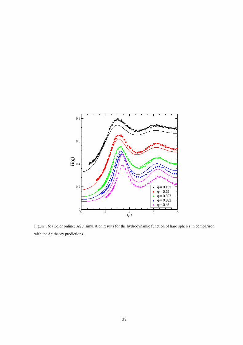
φ = 0.153φ = 0.25φ = 0.327φ = 0.382φ = 0.45

Figure 16: (Color online) ASD simulation results for the hydrodynamic function of hard spheres in comparison

with the δγ theory predictions.

37

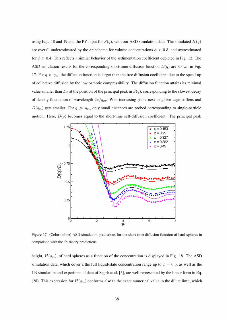
using Eqs. 18 and 19 and the PY input for S(q), with our ASD simulation data. The simulated H(q)

are overall underestimated by the δγ scheme for volume concentrations φ < 0.3, and overestimated

for φ > 0.4. This reflects a similar behavior of the sedimentation coefficient depicted in Fig. 12. The

ASD simulation results for the corresponding short-time diffusion function D(q) are shown in Fig.

17. For q ¿ qm, the diffusion function is larger than the free diffusion coefficient due to the speed-up

of collective diffusion by the low osmotic compressibility. The diffusion function attains its minimal

value smaller than D0 at the position of the principal peak in S(q), corresponding to the slowest decay

of density fluctuation of wavelength 2π/qm. With increasing φ the next-neighbor cage stiffens and

D(qm) gets smaller. For q À qm, only small distances are probed corresponding to single-particle

motion: Here, D(q) becomes equal to the short-time self-diffusion coefficient. The principal peak

0 2 4 6 8qa

0

0.25

0.5

0.75

1

1.25

D(q

)/D

0

φ = 0.153φ = 0.25φ = 0.327φ = 0.382φ = 0.45

Figure 17: (Color online) ASD simulation predictions for the short-time diffusion function of hard spheres in

comparison with the δγ theory predictions.

height, H(qm), of hard spheres as a function of the concentration is displayed in Fig. 18. The ASD

simulation data, which cover a the full liquid-state concentration range up to φ = 0.5, as well as the

LB simulation and experimental data of Segre et al. [5], are well represented by the linear form in Eq.

(28). This expression for H(qm) conforms also to the exact numerical value in the dilute limit, which

38

we have determined using the exact numerical form of the 2-body hydrodynamic mobilities. Segre et

al. [5] give a polynomial fitting formula, D0/D(qm)LB = 1−2φ+58φ2−220φ3+347φ4 that describes

their LB data for D(qm) within 4% of accuracy for volume fractions φ > 0.1. Combining this with Eq.

(30), a LB fitting formula for H(qm) is obtained in overall good agreement with Eq. (28) provided that

φ > 0.13. The linear concentration-scaling of H(qm), valid in the whole fluid regime, is an empirical

finding which we can not explain so far in terms of a simple physical picture. Like in sedimentation

and collective diffusion, the δγ-theory underestimates H(qm) at smaller φ, and overestimates it for

φ > 0.4. The analytic result for the cage diffusion coefficient, D(qm), defined by the ratio of Eqs.

0 0.1 0.2 0.3 0.4 0.5φ

0.2

0.4

0.6

0.8

1

H(q

m)

ASD1 - 1.35 φS(q

m)VW-fit

/ (D0/D(q

m))

LB

δγ theoryEXP: Segre (1995)2-Body HI

Figure 18: (Color online) Peak height, H(qm), of the hydrodynamic function of hard spheres. ASD simulation

data are compared with the LB predictions of Behrend et al. [5], the δγ theory with PY input, experimental data

of Segre et al [5], and the empirical expression 1− 1.35φ in Eq. (28).

(28) and (30), is seen in Fig. 19 to be in excellent agreement with the experimental data of Segre et

al. [5], and our simulation data. This reflects again the accuracy of Eq. (28) in describing the peak

height of the hydrodynamic function of hard spheres.

ASD simulation results for the H(q) of a charge-stabilized suspension in dependence on the vol-

ume fraction, and the amount of added electrolyte, are included in Figs. 20 and 21, respectively.

According to Fig. 20, the q-dependence of H(q) is well captured by the δγ scheme, although

39

0 0.1 0.2 0.3 0.4 0.5φ

0

0.2

0.4

0.6

0.8

1

D(q

m)/

D0

ASD(1 - 1.35 φ)/(1 + 0.664 φ g(2a

+))

Exp.: Segre et al. (1995)

Figure 19: (Color online) Cage diffusion coefficient, D(qm), of colloidal hard spheres versus volume fraction.

The analytic expression for D(qm), defined by the ratio of Eqs. (28) and (30), is tested against ASD simulation

data, and the experimental data of Segre et al. [5].

0 1 2 3 4

qa

0.4

0.6

0.8

1

1.2

H(q

)

φ = 0.0001φ = 0.005φ = 0.055φ = 0.105

Figure 20: (Color online) ASD-simulated hydrodynamic function H(q) of charged spheres at zero added salt

content, in dependence on φ. The δγ theory result (dashed lines) and the self-part corrected δγ theory result

(solid lines) are included for comparison.

40

its predictions are consistently lower than the simulation data. The differences between ASD and

δγ theory become larger with increasing φ and decreasing salt content. The underestimation of the

true H(q) by the zeroth-order δγ scheme is mainly due to the hard-sphere approximation of Ds. It’s

accuracy is improved when, in place of the δγ−Ds, the simulated short-time self-diffusion coefficient

is used, which is larger than the corresponding hard-sphere value. The resulting upward shift of the

original δγ scheme H(q) leads to good overall agreement with the simulation data (see Fig. 20).

The δγ results for H(q) shown in the figure have been obtained using an integral equation S(q) whose

principal peak height has been fitted to the ASD peak height for each system, by adjusting the value for

the charge number Z. Note here that even the RY scheme underestimates to some extent the magnitude

of S(qm) in the case of dense, deionized systems (see Fig. 4).

With increasing salt content, the undulations in H(q) get smaller, reflecting a similar behavior

in S(q) and g(r) (see Fig. 21). Both H(qm) and H(q À qm) = Ds/D0 decrease with increasing

salinity towards the hard-sphere limiting values, and qm is shifted to larger values. The sedimentation

coefficient H(0), however, increases with increasing salt content.

0 1 2 3 4 5 6

qa

0.2

0.4

0.6

0.8

1

H(q

)

ns

= 1.0x10-6

M

ns

= 2.5x10-6

M

ns

= 5.0x10-6

M

ns

= 1.0x10-5

M

ns

= 1.0x10-4

M

Figure 21: (Color online) ASD-simulated H(q) of charged spheres at φ = 0.15, in dependence on the amount

of added 1-1 electrolyte as indicated.

All our ASD simulation results, and analytic theory including the δγ scheme, are in accord with

41

the generic ordering relations, for a given φ,

HCS(qm) > HHS(qm) ,

DCSs > DHS

s ,

UCSs < HHS , (46)

valid for charge-stabilized systems that can be described by the OMF model. Here, CS and HS are the

labels for charged and hard spheres, respectively. For systems with added salt, the values of these prop-

erties are always located in between the zero-salt and infinite-salt (zero-charge) limiting values. Recent

short-time scattering experiments on charge-stabilized systems so different as apoferritin proteins in

water [6], aqueous suspensions of fluorinated latex spheres [15], and silica spheres in DMF [96], con-

firm the validity of these ordering relations without any exceptions.

Depending on the system parameters under consideration, the concentration dependence of H(qm)

can vary substantially. For weakly charged spheres, or charge-stabilized suspensions at high salinity,

H(qm) decreases monotonically in φ similar to hard spheres. For strongly charged spheres at low salin-

ity, on the other hand, H(qm) increases first sub-linearly in φ in accord with eq. (36). At some larger

value of φ, H(qm) passes through a maximum and declines subsequently when φ is further increased.

A point in case is given by the salt-free system discussed in Fig. 20. For a thorough comparison

of simulations, δγ scheme calculations and experimental results on the concentration dependence of

H(qm) we refer to [15].

The particle radius a is the only static and dynamic length scale characterizing colloidal hard-

sphere suspensions. This leads to the approximate existence of an isobestic point, i.e., a wave number

qa ≈ 4.02 located to the right of the main structure factor peak, where both S(q) and H(q)×D0/Ds,

and hence also D(q)/Ds, attain the value one essentially independent of concentration. In fact, the

corresponding q-value for φ = 0.185 is slightly smaller, and moves towards 4.02 with increasing φ.

The existence of such an isobestic point for hard spheres is shown in Fig. 22, which includes ASD

simulation data for various values of φ. The horizontal lines quantify the infinite-q values of S(q),

D(q)/D0 and H(q), respectively, at the indicated volume fractions.

A suggestion due to Pusey [97] is that self-diffusion can be probed approximately at a wave number

q∗ > qm, where S(q∗) = 1. The underlying assumption is that at such a q∗ where the distinct structure

factor Sd(q) = S(q) − 1 is zero, also it’s time-dependent generalization Sd(q, t) = S(q, t) − G(q, t)

42

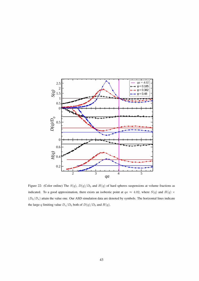
0

0.5

1

1.5

2

2.5

S(q)

qa = 4.02φ = 0.185φ = 0.382φ = 0.48

0

0.5

D(q

)/D

0

2 3 4 5qa

0.2

0.4

0.6

H(q

)

Figure 22: (Color online) The S(q), D(q)/D0 and H(q) of hard spheres suspensions at volume fractions as

indicated. To a good approximation, there exists an isobestic point at qa ≈ 4.02, where S(q) and H(q) ×(D0/Ds) attain the value one. Our ASD simulation data are denoted by symbols. The horizontal lines indicate

the large-q limiting value Ds/D0 both of D(q)/D0 and H(q).

43

is small, now in comparison to the self-intermediate scattering function G(q, t) (with G(q, 0) = 1),

which describes self-diffusion [2, 3]. If this assumption is valid approximately, then D(q∗)/D0 =

H(q∗) ≈ Ds/D0. For hard spheres, this assumption has been corroborated also by LB simulations

and δγ theory [5]. Our ASD simulation data on hard spheres depicted in the figure confirm this finding

additionally. At all φ considered, the difference between Ds/D0 and D(q∗)/D0 = H(q∗) is less than

five percent.

Unlike hard spheres, de-ionized suspensions of strongly charged spheres have at least two char-

acteristic length scales, namely the geometric mean particle distance, n−1/3, and the hydrodynamic

radius a. Therefore, in these systems, there is no isobestic point in S(q) even when it is plotted versus

q × n−1/3. The non-existence of such a concentration-independent intersection point is illustrated in

Fig. 23, which shows ASD results for de-ionized systems at several values of φ. Even though there

are no isobestic points, the ASD simulations show that the short-time self-diffusion coefficient Ds of

charged spheres can be estimated approximately, like in hard-sphere suspensions, by the D(q) for a

wave number q∗ > qm where S(q∗) = 1. For all the systems considered, and similar to the hard-sphere

case, we find the difference between Ds/D0 and H(q∗) to be smaller than five percent.

3.7 Short-time generalized Stokes-Einstein relations

Having discussed the behavior of various short-time properties, we are in the position to examine the

validity of the short-time GSE relations in Eqs. (14), (15) and (16). Fig. 24 provides a test of these

relations for hard spheres. It shows our ASD simulation data for Ds, Dr and D(qm), combined with

the ASD data for η∞. The solid lines are analytic results using Eq. (27) for η∞, in combination with

Eqs. (25), (21), (28), and (30) for Ds (red line), Dr (blue line), and D(qm)/D0 = H(qm)/S(qm)

(black line), respectively. The orange curve is the result of combining the empirical Lionberger-Russel

relations Eq. (26) for η∞ and Eq. (25) for Ds. The so-obtained analytic results are in rather good

accord with the simulation data. For a GSE relation to be valid, the corresponding curve in Fig. 24

should be horizontal and equal to one. It is noted from the figure that the GSE relation involving Dr

is strongly violated for non-zero concentrations. The GSE relation for Ds, on the other hand, is less

strongly violated, with η∞/η0 lying above D0/Ds for all non-zero concentrations. The monotonic rise

of (η∞/η0) × (Ds/D0) with increasing φ is overall well captured, up to φ = 0.5, by the first-order

virial form 1 + 0.67 φ obtained from Eqs. (20) and (23). According to second-order δγ theory, the

44

0

0.5

1

1.5

2

2.5

S(q)

φ = 0.0001φ = 0.005φ = 0.055φ = 0.105

0.5

1

D(q

)/D

0

0 1 2 3qa

0.8

1

1.2

H(q

)

Figure 23: (Color online) The S(q), D(q)/D0 and H(qm) of de-ionized suspensions of charged spheres at

volume fractions as indicated. In these systems, there are no isobestic points. The ASD simulation data are

denoted by the symbols. The horizontal lines are the values for Ds/D0 at the indicated concentrations.

45

0 0.1 0.2 0.3 0.4 0.5φ

1.0

1.5

2.0

D(qm

)/D0

× η∞/η0D

s/D

0× η∞/η0

Dr/D

0× η∞/η0

Figure 24: (Color online) ASD simulation test of the generalized SE relations in Eqs. (14), (15) and (16) for

the hard-sphere case. Symbols: ASD simulation data. Solid lines: analytic results as explained in the text.

Dashed-dotted line: 2nd-order δγ theory prediction for the GSE relation invoking Ds [43].

46

GSE relation for Ds should be violated to some extent (see Fig. 4 in [43]), leading to the prediction

that Ds/D0 > η0/η∞, in qualitative accord with the simulation results. The red curve in Fig. 24

overestimates the simulation data for Ds × η∞ at smaller φ, and it shows a downswing for φ > 0.5.

This is explained by the fact that, at smaller φ, Eq. (25) overestimates the simulation data for Ds to

some extent, and it predicts a too strong decline of Ds for φ > 0.5. The orange curve, on the other

hand, is in better overall agreement with the simulation data, reflecting a fortuitous cancellation of

deviations of the Lionberger-Russel expressions for Ds and η∞ from the simulation data (see Figs. 7

and 10).

Using the SD and ASD methods, Brady et al. have computed the η∞, Ds and η of hard spheres

even above the freezing point, on assuming that the dispersion can be maintained in a non-crystalline,

disordered and metastable state up to random close packing. We have not include their data since,

within the liquid phase regime considered in the present paper, they fully agree with our ASD data,

verifying thus the correctness of the ASD scheme with Brownian forces included for the short-time

dynamics of hard spheres. For concentrations φ > 0.6 where random closed packing is approached,

and on ignoring higher-order moment contributions, Sierou and Brady [20] observe a linear scaling of

Ds(φ) as function of the inverse high-frequency viscosity, which provides evidence that Ds ∝ 1/η∞

in the limit φ → φrcp. These simulations suggest that Ds vanishes at φrcp in a manner inversely

proportional to η∞. For volume fractions below freezing, however, the physical mechanisms of self-

diffusion and viscosity are clearly distinguishable from each other, and the GSE relation for Ds is

violated to some extent, as quantified roughly by Ds(φ)/D0 ≈ (1+0.67φ)×η0/η∞(φ) (see also [18]

and [52]).

The GSE relation for the cage diffusion coefficient, D(qm), of hard spheres is obeyed to a better

degree of accuracy than the one for Ds. Interestingly enough, the opposite trend is found for de-

ionized suspensions of strongly charged spheres (see Fig. 25). Here, the GSE relation for D(qm)

is most strongly violated, for all values of φ considered, whereas the GSE for Ds works decently

well. This reflects that, different from η∞, D(qm) is highly sensitive to system parameters such as the

particle charge and ionic strength, in particular through its explicit dependence on S(qm). The black

diamonds are the ASD results for D(qm)×η∞, obtained for a less strongly correlated deionized system

with system parameters identical to the ones used for the inset of Fig. 11, that characterize a system

which remains fluid up to φ ≈ 0.3. The counterion-dominated electrostatic screening in deionized

47

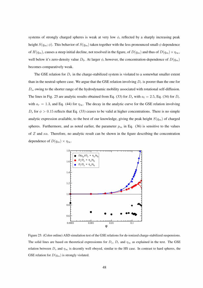
systems of strongly charged spheres is weak at very low φ, reflected by a sharply increasing peak

height S(qm; φ). This behavior of S(qm) taken together with the less pronounced small-φ dependence

of H(qm), causes a steep initial decline, not resolved in the figure, of D(qm) and thus of D(qm)×η∞,

well below it’s zero-density value D0. At larger φ, however, the concentration-dependence of D(qm)

becomes comparatively weak.

The GSE relation for Dr in the charge-stabilized system is violated to a somewhat smaller extent

than in the neutral-sphere case. We argue that the GSE relation involving Dr is poorer than the one for

Ds, owing to the shorter range of the hydrodynamic mobility associated with rotational self-diffusion.

The lines in Fig. 25 are analytic results obtained from Eq. (33) for Ds with at = 2.5, Eq. (34) for Dr

with ar = 1.3, and Eq. (44) for η∞. The decay in the analytic curve for the GSE relation involving

Ds for φ > 0.15 reflects that Eq. (33) ceases to be valid at higher concentrations. There is no simple

analytic expression available, to the best of our knowledge, giving the peak height S(qm) of charged

spheres. Furthermore, and as noted earlier, the parameter pm in Eq. (36) is sensitive to the values

of Z and κa. Therefore, no analytic result can be shown in the figure describing the concentration

dependence of D(qm)× η∞.

0.0001 0.001 0.01 0.1φ

0.6

0.8

1.0

1.2

1.4

1.6

1.8

D(qm

)/D0

× η∞/η0

Ds/D

0× η∞/η0

Dr/D

0× η∞/η0

Figure 25: (Color online) ASD simulation test of the GSE relations for de-ionized charge-stabilized suspensions.

The solid lines are based on theoretical expressionns for Ds, Dr and η∞ as explained in the text. The GSE

relation between Ds and η∞ is decently well obeyed, similar to the HS case. In contrast to hard spheres, the

GSE relation for D(qm) is strongly violated.

48

We conclude our discussion of short-time GSE relations by noting that the ordering relation Ds >

kBT/(6π η∞ a) is valid both for de-ionized suspensions and neutral hard spheres, in agreement with

experiments of Bergenholtz et al., where η∞ and Ds have been measured for various ionic strengths

and concentrations [76].

4 CONCLUDING REMARKS

This work includes the first comprehensive (accelerated) SD computer simulation study on the short-

time dynamic properties of charge-stabilized suspensions. Using an extension of the ASD simulation

method to the OMF model of charged colloidal spheres, numerous short-time quantities have been cal-

culated including collective and self-diffusion coefficients, sedimentation coefficient, high-frequency

limiting viscosity, and hydrodynamic functions. The short-time dynamics of colloidal hard spheres has

been part of this study in order to highlight the qualitative differences between low-salinity charge-

stabilized suspensions, and hard-sphere-like systems which have a high salt content. The range of

validity, and the degree of accuracy, of various analytic short-time expressions have been explored

through comparison with our ASD simulation data in the case of charged spheres and, for neutral hard

spheres, also with earlier SD and ASD simulation results of Brady and coworkers, and LB simulation

data of Ladd and Behrend et al. The assessment of the quality of these handy-to-use analytic expres-

sions is a necessary prerequisite for the experimentalist who wishes to use these expressions for data

interpretation, and in any theory on colloidal long-time dynamics where short-time properties are the

basic input.

For hard spheres, in particular, we have assessed the concentration range where the currently avail-

able truncated virial expansion results by Cichocki and coworkers are valid. Moreover, we have shown

that the expressions in Eqs. (28), (30) and (27) provide excellent descriptions of H(qm), D(qm) and

η∞ in the whole fluid regime.

For de-ionized suspensions characterized by long-range repulsive forces, simple physical argu-

ments based on the dominance of far-field HI in these systems, and the φ−1/3 concentration scaling

of the next-neighbor shell diameter, have led to short-time expressions showing a non-linear or even

fractal concentration dependence. The present ASD simulation study has allowed us to quantify the

accuracy of these expressions. We have found that most of them apply quantitatively in a restricted

φ-range only, as one can expect from the assumptions made in their derivation. Eqs. (34) and (44)

49

for Dr and η∞, however, are valid to good accuracy even for fluid systems with very strong particle

correlations. For low-salt systems, the simulations confirm the values of the exponents in the Eqs.

(33)-(36) which are independent of the details of the interaction parameters.

The ASD simulation study of isobestic points and, more specifically, of wave numbers where

S(q) = 1, has allowed us to quantify the experimental error made in determining Ds through dynamic

light scattering measurements at such points. This is of relevance for numerous colloidal systems

where the large-q regime is not accessible experimentally, and where partial index matching techniques

are not applicable.

Various short-time GSE relations have been examined. We find that rotational self-diffusion and, to

a lesser extent, translational self-diffusion is larger than predicted by the corresponding GSE relations.

The amount by which a GSE relation is violated depends sensitively on the range of the electrostatic

interaction. For example, the GSE relation for the cage diffusion coefficient is valid in the case of hard

spheres to decently good accuracy, but is strongly violated in de-ionized suspensions. The general

trends in the behavior of Ds and η∞, as predicted by the ASD simulations, are in agreement with the

experimental findings on charge-stabilized dispersions.

Furthermore, our simulations show that the δγ theory of Beenakker and Mazur, initially applied to

hard spheres only, remains useful in the case of charged spheres, where it can be used for short-time

calculations on a semi-quantitative level of accuracy. In calculating H(q), the accuracy of the zeroth-

order δγ theory is improved when combined with a more accurate calculation of the self-part Ds based,

e.g., on a rooted cluster approximation for charged spheres. The δγ theory is particularly suited for

systems of intermediate salt content, where no simple short-time analytic expressions are available, and

where a high data throughput is required which makes simulation calculations prohibitively expensive.

The basis of our ASD simulation study has been the OMF model describing dressed spherical

macroions. To date this is the most widely used model for charge-stabilized suspensions of particles

with negligibly small dispersion attractions. The OMF model has been extended in various ways to ac-

count for macroion charge-renormalization effects arising from the quasi-condensation of counterions

near strongly charged colloid surfaces, and for electrokinetic effects caused by the non-instantaneous

dynamic response of the electrolyte atmosphere formed around each colloidal particle. Recent calcula-

tions based on a mode coupling scheme applied to the primitive model that includes hydrodynamic in-

teractions between all ionic species show that the electrokinetic influence on the colloidal self-diffusion

50

is quite small, and ceases with increasing volume fraction [11]. The effect of the electrolyte dynamics

is somewhat stronger when collective diffusion is considered, where it can cause a reduction in Dc by

several percent [6]. This reduction is most pronounced at low salinity, but is becomes weaker with in-

creasing colloid-microion size ratio. However, the very small values of H(q) purportedly measured in

recent experiments on certain de-ionized suspensions by Grubel, Robert and coworkers [34,48,98], can

not be explained by this secondary electrokinetic effect which diminishes at large macroion-microion

size ratios. These authors find values of H(qm) that are roughly by a factor of two smaller than the

peak heights obtained from our simulation calculations [6, 15], with the latter being consistent with

experimental data for H(q), Dc, Us and Ds obtained by other groups [49, 50, 71, 75, 76, 99].

The present paper was concerned with monodisperse suspensions of charged colloidal spheres

with negligible attractive forces. In future extensions of this simulation work, we will address the

short-time diffusion and rheology of particles with a non-negligible attractive interaction part such as

globular lysozyme proteins, and we will study the dynamics in binary colloidal mixtures.

Acknowledgments

This work has been supported by the Deutsche Forschungsgemeinschaft (SFB-TR6), and by CON-

ICET, FONCYT (PICT 2005-33691) and SECYT-UNC, Argentina. A.J. Banchio expresses his deep

gratitude to Prof. John Brady, who is co-developer of the ASD code for Brownian spheres. Without his

contribution, the present simulation work would not have been possible. We gratefully acknowledge

discussions with J.K.G. Dhont, J. Gapinski, Ch. Gogelein, M. McPhie, and A. Patkowski.

References

[1] W.B. Russel, D.A. Saville and W.R. Schowalter, Colloidal Dispersions (Cambridge University

Press, Cambridge, 1989).

[2] P.N. Pusey, in Liquids, Freezing and the Glass Transition, edited by J.-P. Hansen, D. Levesque

and J. Zinn-Justin (Elsevier, Amsterdam, 1991) pp. 763-942.

[3] G. Nagele, Phys. Rep. 272, 215 (1996).

[4] J.K.G. Dhont, An Introduction to Dynamics of Colloids (Elsevier, Amsterdam, 1996).

51

[5] P. N. Segre, O. P. Behrend and P. N. Pusey, Phys. Rev. E 52, 5070 (1995).

[6] J. Gapinski, A. Wilk, A. Patkowski, W. Haussler, A.J. Banchio, R. Pecora and G. Nagele, J.

Chem. Phys. 123, 1054708 (2005).

[7] A. Evilevitch, V. Lobaskin, U. Olsson, P. Linse and P. Schurtenberger, Langmuir 17, 1043 (2001).

[8] G. Nagele and P. Baur, Europhys. Lett. 38, 557 (1997).

[9] K. Zahn, J.M. Mendez-Alcaraz and G. Maret, Phys. Rev. Lett. 79, 175 (1997).

[10] W. Hartl, J. Wagner, Ch. Beck, F. Gierschner and R. Hempelmann, J. Phys.: Condens. Matter 12,

A287 (2000).

[11] M.G. McPhie and G. Nagele, J. Chem. Phys. 127, 034906 (2007).

[12] M.G. McPhie and G. Nagele, J. Phys.: Condens. Matter 16, S4021 (2004).

[13] A.J. Banchio and J.F. Brady, J. Chem. Phys. 118, 10323 (2003)

[14] A.J. Banchio, J. Gapinski, A. Patkowski, W. Haussler, A. Fluerasu, S. Saccana, P. Holmqvist, G.

Meier, M.P. Lettinga and G. Nagele, Phys. Rev. Lett. 96, 138303 (2006).

[15] J. Gapinski, A. Patkowski, A.J. Banchio, P. Holmqvist, G. Meier, M.P. Lettinga and G. Nagele,

J. Chem. Phys. 126, 104905 (2007).

[16] R.J. Philips, J.F. Brady and G. Bossis, Phys. Fluids 31, 3462 (1988).

[17] J.F. Brady, R.J. Phillips, J.C. Lester and G. Bossis, J. Fluid Mech. 195, 257 (1988).

[18] J.F. Brady, Curr. Opin. Colloid Interface Sci. 1, 472 (1996).

[19] D.R. Ross and J.F. Brady, J. Fluid Mech. 407, 167 (2000).

[20] A. Sierou and J.F. Brady, J. Fluid Mech. 448, 115 (2001).

[21] A.J.C. Ladd, J. Chem. Phys. 93, 3484 (1990).

[22] A.J.C. Ladd, H. Gang, J.X. Zhu and D.A. Weitz, Phys. Rev. E 52, 6550 (1995).

[23] O.P. Behrend, Phys. Rev. E 52, 1164 (1995).

52

[24] O.P. Behrend, Ph.D. thesis, University of Edinburgh (1995).

[25] M.H.J. Hagen, D. Frenkel and C.P. Lowe, Physica A 272 376 (1999).

[26] M.W. Heemels, M.H.J. Hagen and C.P. Lowe, J. Comput. Phys. 164 48 (2000).

[27] A.J.C. Ladd, J. Fluid Mech. 271, 285 (1994), 271, 311 (1994).

[28] I. Snook, W. van Megen and R.J.A. Tough, J. Chem. Phys. 78, 5825 (1983).

[29] W. van Megen and I. Snook, J. Chem. Soc., Faraday Trans. 2 80, 383 (1984).

[30] W. van Megen and I. Snook, J. Chem. Phys. 88, 1185 (1987).

[31] S. Walrand, L. Belloni and M. Drifford, J. Physique 47, 1565 (1986).

[32] C.W.J. Beenakker and P. Mazur, Physica 126 A, 349 (1984).

[33] J.F. Brady and L.J. Durlofsky, Phys. Fluids 31, 717 (1988).

[34] D.O. Riese, G.H. Wegdam, W.L. Vos, R. Sprik, D. Fenistein, J.H.H. Bongaerts and G. Grubel,

Phys. Rev. Lett. 85, 5460 (2000).

[35] B. Cichocki, M.L. Ekiel-Jezewska and E. Wajnryb, J. Chem. Phys. 111, 3265 (1999).

[36] B. Cichocki, M.L. Ekiel-Jezewska, P. Szymczak and E. Wajnryb, J. Chem. Phys. 117, 1231

(2002).

[37] B. Cichocki, M.L. Ekiel-Jezewska and E. Wajnryb, J. Chem. Phys. 119, 606 (2003).

[38] M. Watzlawek and G. Nagele, Phys. Rev. E 56, 1258 (1997).

[39] H. Zhang and G. Nagele, J. Chem. Phys. 117, 5908 (2002).

[40] G.H. Koenderink, H. Zhang, D.G.A.L. Aarts, M.P. Lettinga, A.P. Philipse and G. Nagele, Faraday

Discuss. 123 335 (2002).

[41] C.W.J. Beenakker and P. Mazur, Phys. Lett. A 98, 22 (1983).

[42] C.W.J. Beenakker, Ph.D. thesis, University of Leiden (1984).

[43] C.W.J. Beenakker, Physica A 128, 48 (1984).

53

[44] R.L. Treloar and A.J. Masters, Mol. Phys. 67, 1273 (1989).

[45] U. Genz and R. Klein, Physica A 171, 26 (1991).

[46] G. Nagele, B. Steininger, U. Genz and R. Klein, Physica Scripta T 55, 119 (1994).

[47] G. Nagele, B. Mandl and R. Klein, Progr Colloid Polym Sci 98, 117 (1995).

[48] A. Robert, Ph.D. thesis, Universite Joseph Fourier, Grenoble, France (2001).

[49] L.F. Rojas, R. Vavrin, C. Urban, J. Kohlbrecher, A. Stradner, F. Scheffold and P. Schurtenberger,

Faraday Discuss 123, 385 (2003).

[50] L.F. Rojas, Ph.D. thesis, University of Fribourg, Switzerland (2004).

[51] E.G.D. Cohen, R. Verberg and I.M. de Schepper, Physica A 251, 251 (1998).

[52] A.J. Banchio, G. Nagele and J. Bergenholtz, J. Chem. Phys. 111, 8721 (1999).

[53] A.J. Banchio, J. Bergenholtz and G. Nagele, Phys. Rev. Lett. 82, 1792 (1999).

[54] M. Fuchs and M.R. Mayr, Phys. Rev. E 60, 5742 (1999).

[55] A.R. Denton, Phys. Rev. E 62, 3855 (2000).

[56] J.W. Verwey and J.T.G. Overbeek, Theory of the Stability of Lyotropic Colloids (Elsevier. Ams-

terdam, 1948).

[57] L. Belloni, J. Chem. Phys. 85, 519 (1986).

[58] W.B. Russel and D.W. Benzing, J. Colloid Interface Sci. 83, 163 (1981).

[59] E. Trizac, L. Bocquet, M. Aubouy and H.H. von Grunberg, Langmuir 19, 4027 (2003).

[60] B. Beresford-Smith, D.Y. Chan abd D.J. Mitchell, J. Colloid Interface Sci. 105, 216 (1984).

[61] A. Diehl and Y. Levin, J. Chem. Phys. 121, 12100 (2004).

[62] W.L. Hsin, T.Y. Wang, Y.J. Sheng and H.K. Tsao, J. Chem. Phys. 121, 5494 (2004).

[63] S. Pianegonda, E. Trizac and Y. Levin, J. Chem. Phys. 126, 014702 (2007).

54

[64] A.P. Hynninen and M. Dijkstra, J. Chem. Phys. 123, 244902 (2005).

[65] T. Kreer, J. Horbach and A. Chatterji, Phys. Rev. E 74, 021401 (2006).

[66] J.P. Hansen and I.R. McDonald, Theory of Simple Liquids, (2nd Edition, Academic Press, Lon-

don, 1986).

[67] F.J. Rogers and D.A. Young, Phys. Rev. A 30, 999 (1984).

[68] J.P. Hansen and J.B. Hayter, Mol. Phys. 46 651 (1982).

[69] G. Nagele, The Physics of Colloidal Soft Matter, Lecture Notes 14, Institute of Fundamental

Technological Research (Polish Academy of Sciences publication, Warsaw, 2004).

[70] R.B. Jones and P.N. Pusey, Annu. Rev. Phys. Chem. 42, 137 (1991).

[71] J.K. Phalakornkul, A.P. Gast, R. Pecora, G. Nagele, A. Ferrante, B. Mandl-Steininger, and R.

Klein, Phys. Rev. E 54, 661 (1996).

[72] D.M.E. Thies-Weesie, A.P. Philipse, G. Nagele, B. Steininger and R. Klein, J. Colloid Interface

Sci. 176, 43 (1995).

[73] E. Wajnryb, P. Szymczak and B. Cichocki, Physica A 335, 339 (2004).

[74] V. Degiorgio, R. Piazza and R.B. Jones, Phys. Rev. E 52, 2707 (1995).

[75] E. Overbeck, C. Sinn and M. Watzlawek, Phys. Rev. E 60, 1936 (1999).

[76] J. Bergenholtz, F.M. Horn, W. Richtering, N. Willenbacher and N.J. Wagner, Phys. Rev. E 58,

R4088 (1998).

[77] G. Nagele, J. Phys.: Condens. Matter 15, S407 (2003).

[78] J. Zhang and X.Y. Liu, J. Chem. Phys. 119, 10972 (2003).

[79] B. Cichocki and B.U. Felderhof, J. Chem. Phys. 93, 4427 (1990).

[80] K.F. Seefeldt and M.J. Solomon, Phys. Rev. E 67, 050402(R) (2003).

[81] A.T.J.M. Woutersen, J. Mellema, C. Blom and C.G. de Kruif, J. Chem. Phys. 101, 542 (1994).

55

[82] R.A. Lionberger and W.B. Russel, J. Rheology 38, 1885 (1994).

[83] H.J.H. Clercx and P.P.J.M. Schram, Phys. Rev. A 45, 860 (1992).

[84] A.J. Banchio, G. Nagele and J. Bergenholtz, J. Chem. Phys. 113, 3381 (2000).

[85] P.N. Segre, S.P. Meeker, P.N. Pusey and W.C.K. Poon, Phys. Rev. Lett. 74, 1250 (1995).

[86] F.-U. Tao, Y. Song and E.A. Mason, Phys. Rev. A 46, 8007 (1992).

[87] M. Watzlawek and G. Nagele, J. Colloid Interface Sci. 214, 170 (1999).

[88] G. Nagele, O. Kellerbauer, R. Krause and R. Klein, Phys. Rev. E 47, 2562 (1993).

[89] W.B. Russel, J. Fluid Mech. 85, 209 (1978).

[90] W. Hartl, Ch. Beck and R. Hempelmann, J. Chem. Phys. 110, 7070 (1999).

[91] M.S. Wertheim, J. Math. Phys. 5, 643 (1964).

[92] F.M. Horn, W. Richtering, J. Bergenholtz, N. Willenbacher and N.J. Wagner, J. Colloid Interface

Sci. 225, 166 (2000).

[93] D.M. Heyes and H. Sigurgeirsson, J. Rheol. 48, 223 (2004).

[94] H. Hasimoto, J. Fluid Mech. 5, 317 (1959).

[95] P.G. Saffman, Stud. Appl. Math. 52, 115 (1973).

[96] J. Gapinski, A. Patkowski, A.J. Banchio, G. Nagele et al., in preparation.

[97] P.N. Pusey, J. Phys. A 11, 119 (1978).

[98] T. Autenrieth, A. Robert, J. Wagner and G. Grubel, J. Appl. Cryst. 40, s250 (2007).

[99] A.P. Philipse and A. Vrij, J. Chem. Phys. 88, 6459 (1988)

56

Figure Captions

Fig. 1 (Color online) Static structure factor of a hard-sphere suspension at various volume fractions φ

as indicated. Comparison between MD simulation data and Rogers-Young (RY), Percus-Yevick (PY)

and Verlet-Weiss corrected Percus-Yevick (PY-VW) integral equation schemes.

Fig. 2 (Color online) Peak value, S(qm), of the hard-sphere static structure factor. MD simulation

data (symbols) are compared with PY calculations and the PY-VW fitting formula in Eq. (30).

Fig. 3 (Color online) Hard-sphere radial distribution function corresponding to Fig. 1. The curves for

φ = 0.40 and 0.20 are shifted to the right by a and 2a, respectively.

Fig. 4 (Color online) Static structure factor of a de-ionized charge-stabilized suspension at volume

fractions as indicated. The MC simulation data (symbols) are compared with Rogers-Young calcula-

tions (solid lines) using identical system parameters, i.e., Z = 100, LB = 5.62 nm and ns = 0.

Fig. 5 (Color online) Concentration dependence of the peak position, qm, of the static structure factor

of de-ionized suspension in units of the particle radius. The green diamonds are the RMSA result for

ns = 0. Blue circles: MC data for ns = 0; Black circles: MC result for a collection of systems with

varying amount of added salt. Red circles: MD data for a system at φ = 0.15 with ns varying from

1 × 10−6 to 1 × 10−4 M. Additionally shown is the peak-position wave number of hard spheres, as

predicted by the Verlet-Weiss corrected PY scheme.

Fig. 6 (Color online) Translational short-time self-diffusion coefficient of hard spheres versus vol-

ume fraction φ. Comparison of the ASD and force multipole simulation data with the zeroth order and

second order δγ theory prediction, the 2nd order virial expansion result of Cichocki et al., the semi-

empirical expression of Lionberger and Russel in Eq. (25), and the experimental data of Segre et al. [5].

Fig. 7 (Color online) Translational short-time self-diffusion coefficient of charged spheres in a salt-

free suspension (labelled by CS) versus the hard-sphere result (HS). The symbols are our ASD simula-

tion results. Green diamonds: hard spheres; blue circles: de-ionized suspension; red circles: transition

57

from a de-ionized system, at φ = 0.15, to a hard-sphere-like system on increasing ns from 1 × 10−6

to 1× 10−4 M; black circles: collection of systems with varying amount of added salt.

Fig. 8 (Color online) Short-time rotational self-diffusion coefficient of hard spheres versus volume

fraction. The symbols are our ASD results and correspond to the ones in Figs. 6 and 7. The ASD data

are compared with Lattice-Boltzmann simulation data of Hagen et al. [25], the truncated virial expan-

sion (in Eq. (21)), and the experimental data of Degiorgio et al. [74]. The 2nd-order virial expression

remains valid up to φ = 0.45.

Fig. 9 (Color online) Short-time rotational self-diffusion coefficient of a de-ionized suspension of

charged spheres (CS), in comparison to the Dr of neutral spheres (HS). The symbols are our ASD

simulation results, with same symbols and color coding as in Fig. 7. The quadratic scaling form in Eq.

(34), which accounts for far-field 3-body HI corrections, remains valid up to remarkably large φ. The

Dr for systems with added salt is bounded from above and below, respectively, by the two limiting

curves describing de-ionized charged-sphere and neutral hard-sphere systems.

Fig. 10 (Color online) High-frequency limiting viscosity, η∞, of colloidal hard spheres versus φ.

Displayed are our ASD simulation data in comparison with the force multipole simulation data of

Ladd [21], the third-order truncated virial expansion result in Eq. (23), the semi-empirical Lionberger-

Russel expression in Eq. (26), the simulation fitting formula of Ladd in Eq. (27), the modified Saito

expression of Cichocki et al. in Eq. (45), and the 2nd order δγ-PY result taken from [43].

Fig. 11 (Color online) High-frequency limiting viscosity of two de-ionized suspensions of charged

spheres (Circles: Z = 100, a = 100 nm, LB = 5.62 nm, ns = 0; diamonds: Z = 70, a = 25 nm,

LB = 0.71 nm, ns = 0 ). The ASD simulation data are overall well described by Eq. (44) which

derives from a schematic model for g(r) using the leading-order far-field HI contribution. For an ex-

panded view of the differences, the inset shows the excess short-time viscosity.

Fig. 12 (Color online) Short-time sedimentation coefficient, Us/U0, of a homogeneous hard-sphere

suspension. The 2nd-order virial and Rotne-Prager approximation results, and the zeroth-order δγ

58

scheme prediction are compared with the accurate computer simulation results of Ladd [21], and LB

simulations of Segre et al. [5]. Note here the strong difference between η0/η∞(φ) and η0/η(φ).

Fig. 13 (Color online) Sedimentation coefficient, Us/U0, of a de-ionized charge-stabilized suspen-

sion versus φ. Experimental data are taken from [50], and compared with the scaling form in Eq. (35)

using as = 1.8. The sedimentation coefficient of hard spheres as described by Eq. (22) is shown for

comparison.

Fig. 14 (Color online) Short-time collective diffusion coefficient, Dc = D(q → 0), of hard spheres.

Comparison between the simulation data of Ladd [21], obtained from dividing the simulated Us/U0

by SCS(0), LB simulation data and dynamic light scattering data of Segre et al. [5], zeroth-order δγ

theory prediction, and the 2nd-order virial result in Eq. (24).

Fig. 15 (Color online) Uncorrected ASD-simulated hydrodynamic function, HN (q), of a charge-

stabilized suspension (lines) with φ = 0.123, Z = 1400, a = 82.5 nm, and LB = 0.71 nm, for

various numbers N of simulated spheres as indicated. The finite-size corrected functions (symbols),

obtained using Eq. (17), collapse on a single curve that is identified as H(q).

Fig. 16 (Color online) ASD simulation results for the hydrodynamic function of hard spheres in

comparison with the δγ theory predictions.

Fig. 17 (Color online) ASD simulation predictions for the short-time diffusion function of hard

spheres in comparison with the δγ theory predictions.

Fig. 18 (Color online) Peak height, H(qm), of the hydrodynamic function of hard spheres. ASD

simulation data are compared with the LB predictions of Behrend et al. [5], the δγ theory with PY

input, experimental data of Segre et al [5], and the empirical expression 1− 1.35φ in Eq. (28).

Fig. 19 (Color online) Cage diffusion coefficient, D(qm), of colloidal hard spheres versus volume

fraction. The analytic expression for D(qm), defined by the ratio of Eqs. (28) and (30), is tested against

59

ASD simulation data, and the experimental data of Segre et al. [5].

Fig. 20 (Color online) ASD-simulated hydrodynamic function H(q) of charged spheres at zero added

salt content, in dependence on φ. The δγ theory result (dashed lines) and the self-part corrected δγ

theory result (solid lines) are included for comparison.

Fig. 21 (Color online) ASD-simulated H(q) of charged spheres at φ = 0.15, in dependence on the

amount of added 1-1 electrolyte as indicated.

Fig. 22 (Color online) The S(q), D(q)/D0 and H(q) of hard spheres suspensions at volume fractions

as indicated. To a good approximation, there exists an isobestic point at qa ≈ 4.02, where S(q) and

H(q) × (D0/Ds) attain the value one. Our ASD simulation data are denoted by symbols. The hori-

zontal lines indicate the large-q limiting value Ds/D0 both of D(q)/D0 and H(q).

Fig. 23 (Color online) The S(q), D(q)/D0 and H(qm) of de-ionized suspensions of charged spheres

at volume fractions as indicated. In these systems, there are no isobestic points. The ASD simulation

data are denoted by the symbols. The horizontal lines are the values for Ds/D0 at the indicated con-

centrations.

Fig. 24 (Color online) ASD simulation test of the generalized SE relations in Eqs. (14), (15) and (16)

for the hard-sphere case. Symbols: ASD simulation data. Solid lines: analytic results as explained in

the text. Dashed-dotted line: 2nd-order δγ theory prediction for the GSE relation invoking Ds [43].

Fig. 25 (Color online) ASD simulation test of the GSE relations for de-ionized charge-stabilized

suspensions. The solid lines are based on theoretical expressionns for Ds, Dr and η∞ as explained in

the text. The GSE relation between Ds and η∞ is decently well obeyed, similar to the HS case. In

contrast to hard spheres, the GSE relation for D(qm) is strongly violated.

60

Figures

Banchio and Nagele – Fig. 1

0 2 4 6qa

0

0.5

1

1.5

2

2.5

3

S(q)

PYRYPY-VWMD

φ = 0.49

φ = 0.40

φ = 0.20

61

Banchio and Nagele – Fig. 2

0 0.1 0.2 0.3 0.4 0.5φ

1

1.5

2

2.5

3

3.5

4

S(q m

)

PYVW-fitMD

62

Banchio and Nagele – Fig. 3

2 3 4 5r/a

0

1

2

3

4

5

6

g(r)

PY-VWRYPYMD

φ = 0.49

φ = 0.40

φ = 0.20

63

Banchio and Nagele – Fig. 4

0 1 2 3 4

qa

0

0.5

1

1.5

2

2.5

3

S(q)

φ = 0.0001φ = 0.005φ = 0.055φ = 0.105RY

64

Banchio and Nagele – Fig. 5

0.0001 0.001 0.01 0.1 1φ

0.1

1

q m a

PY-VW (hard spheres)RMSA (deionized system)

1.095 * 2π [3φ/(4π)]1/3

65

Banchio and Nagele – Fig. 6

0 0.1 0.2 0.3 0.4 0.5φ

0

0.2

0.4

0.6

0.8

1

Ds /D

0

Exp: Segre et al. (1995)Lionberger & Russel (1994)

1 - 1.832φ - 0.219φ2(3-body HI)

Ladd (1990)ASDzeroth-order δγ2nd-order δγ

66

Banchio and Nagele – Fig. 7

0.001 0.01 0.1φ

0.2

0.4

0.6

0.8

1

Ds /D

0

HS: Lionberger & Russel (1994)

CS: 1 - 2.5 φ4/3

67

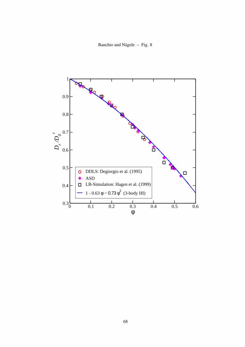
Banchio and Nagele – Fig. 8

0 0.1 0.2 0.3 0.4 0.5 0.6φ

0.3

0.4

0.5

0.6

0.7

0.8

0.9

1

Dr /D

0r

DDLS: Degiorgio et al. (1995)

ASDLB-Simulation: Hagen et al. (1999)

1 - 0.63 φ − 0.73 φ2(3-body HI)

68

Banchio and Nagele – Fig. 9

0.001 0.01 0.1φ

0.8

0.85

0.9

0.95

1

Dr /D

0r

HS: 1 − 0.631 φ − 0.726 φ2

CS: 1 − 1.3 φ2

69

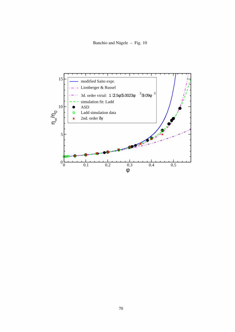
Banchio and Nagele – Fig. 10

0 0.1 0.2 0.3 0.4 0.5φ

0

5

10

15

η ∞/η

0

modified Saito expr.

Lionberger & Russel

3d. order virial: 1 + 2.5φ+ 5.0023φ2+ 9.09φ3

simulation fit: LaddASDLadd simulation data2nd. order δγ

70

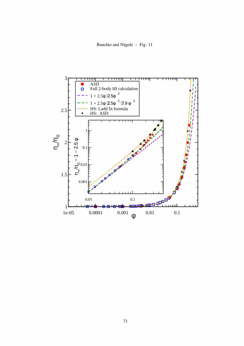
Banchio and Nagele – Fig. 11

1e-05 0.0001 0.001 0.01 0.1φ1

1.5

2

2.5

3

η ∞/η

0

ASDFull 2-body HI calculation

1 + 2.5φ + 2.5φ2

1 + 2.5φ + 2.5φ2 + 7.9 φ3

HS: Ladd fit formulaHS: ASD

0.01 0.1

0.001

0.01

0.1

1

η ∞/η

0 − 1

− 2

.5 φ

71

Banchio and Nagele – Fig. 12

0 0.1 0.2 0.3 0.4 0.5

φ

0

0.2

0.4

0.6

0.8

1

Us/U

0

Simulation Ladd (1990)

δγ - theory

(1-φ)³/(1+2φ) + φ²/5

1 - 6.546φ + 21.918φ²

η0/η∞ (Eq. (27))

η0/η(φ) : HI-rescaled MCT

Simulation Segre et al. (1995)

72

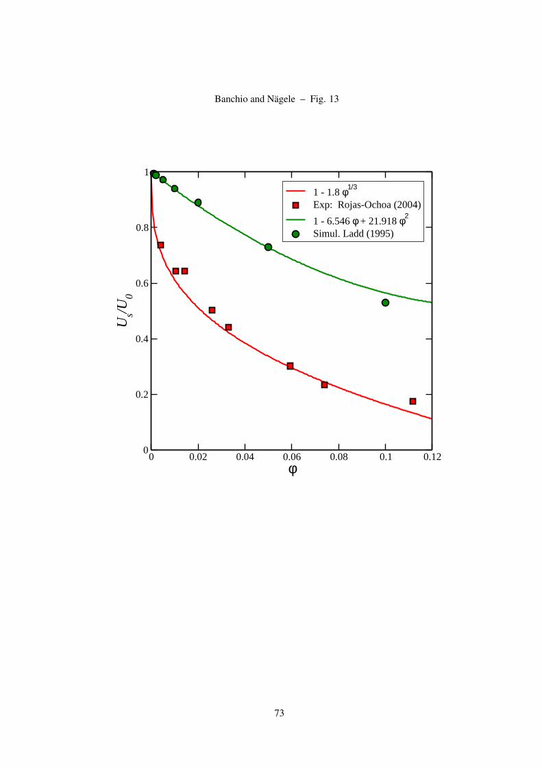
Banchio and Nagele – Fig. 13

0 0.02 0.04 0.06 0.08 0.1 0.12φ

0

0.2

0.4

0.6

0.8

1

Us/U

0

1 - 1.8 φ1/3

Exp: Rojas-Ochoa (2004)

1 - 6.546 φ + 21.918 φ2

Simul. Ladd (1995)

73

Banchio and Nagele – Fig. 14

0 0.1 0.2 0.3 0.4 0.5φ

1

1.5

2

2.5

3

Dc/D

0

δγ theory

1 + 1.454 φ − 0.45 φ2

Ladd-(Us/U

0)/S

CS(0)

Exp.: Segre et al. (1995)

Simulations: Segre et al. (1995)

74

Banchio and Nagele – Fig. 15

0 1 2 3 4 5 6qa

0.4

0.6

0.8

1

H(q

)

ASD - N = 125 - correctedASD - N = 250 - correctedASD - N = 343 - correctedASD - N = 512 - corrected

75

Banchio and Nagele – Fig. 16

0 2 4 6 8qa

0

0.2

0.4

0.6

0.8

H(q

)

φ = 0.153φ = 0.25φ = 0.327φ = 0.382φ = 0.45

76

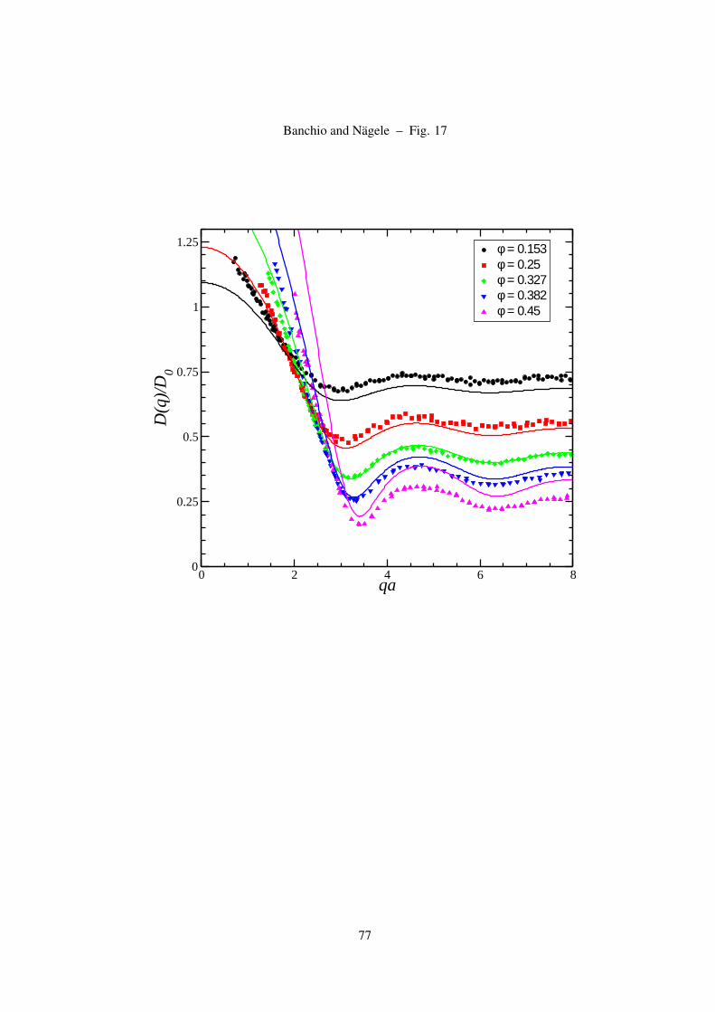
Banchio and Nagele – Fig. 17

0 2 4 6 8qa

0

0.25

0.5

0.75

1

1.25

D(q

)/D

0

φ = 0.153φ = 0.25φ = 0.327φ = 0.382φ = 0.45

77

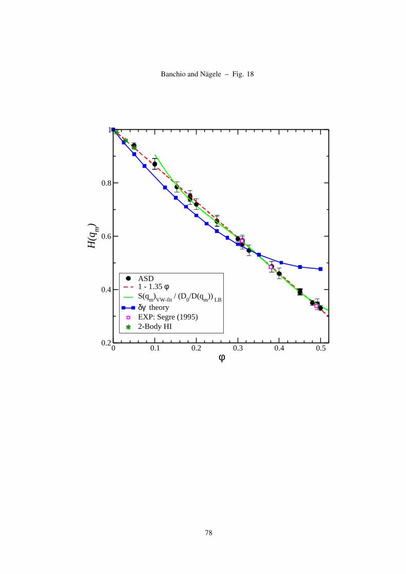
Banchio and Nagele – Fig. 18

0 0.1 0.2 0.3 0.4 0.5φ

0.2

0.4

0.6

0.8

1

H(q

m)

ASD1 - 1.35 φS(q

m)VW-fit

/ (D0/D(q

m))

LB

δγ theoryEXP: Segre (1995)2-Body HI

78

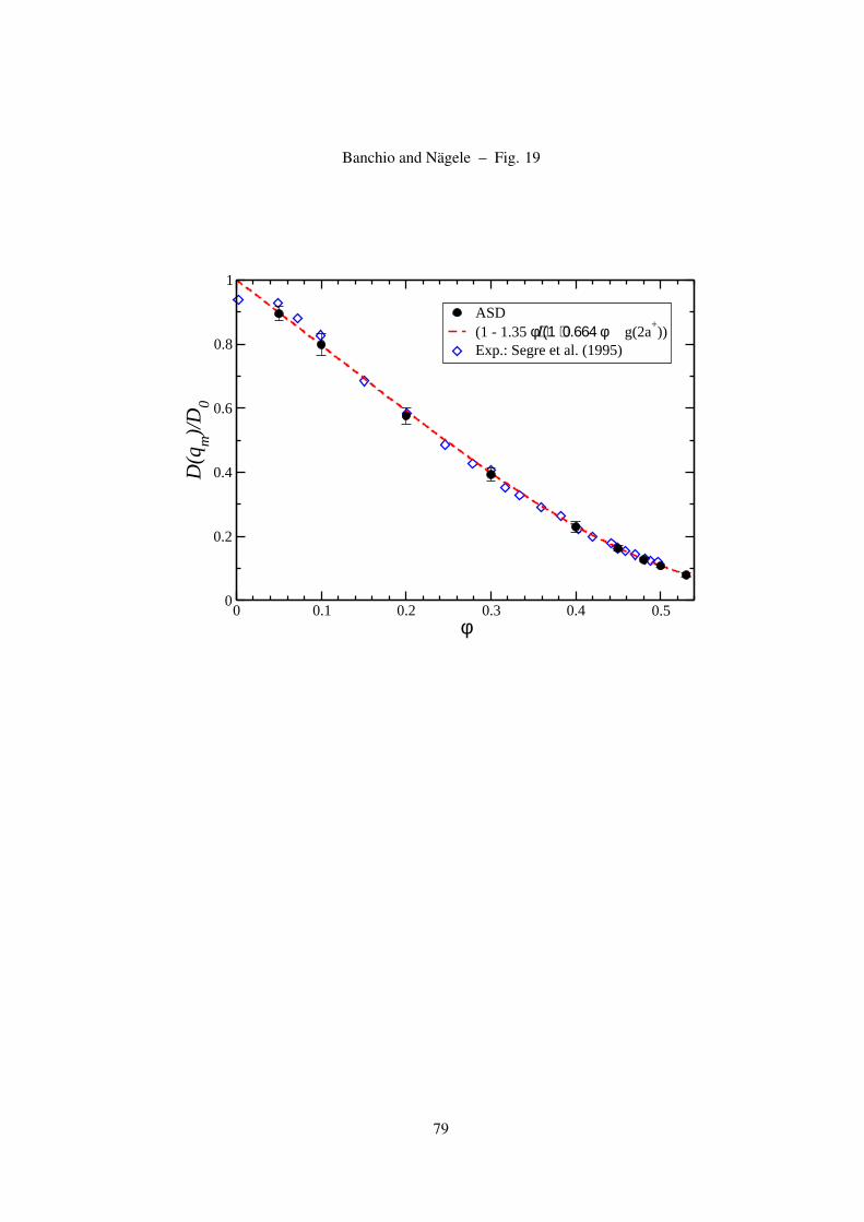
Banchio and Nagele – Fig. 19

0 0.1 0.2 0.3 0.4 0.5φ

0

0.2

0.4

0.6

0.8

1

D(q

m)/

D0

ASD(1 - 1.35 φ)/(1 + 0.664 φ g(2a

+))

Exp.: Segre et al. (1995)

79

Banchio and Nagele – Fig. 20

0 1 2 3 4

qa

0.4

0.6

0.8

1

1.2

H(q

)

φ = 0.0001φ = 0.005φ = 0.055φ = 0.105

80

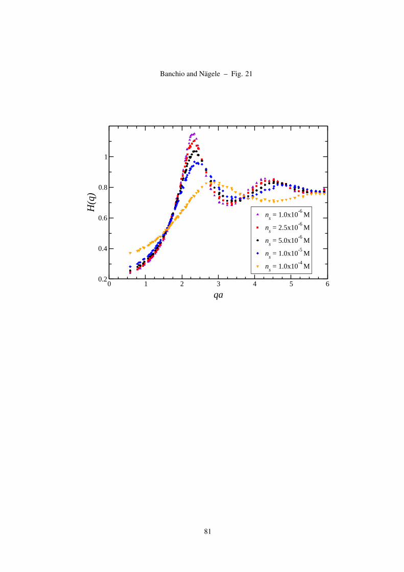
Banchio and Nagele – Fig. 21

0 1 2 3 4 5 6

qa

0.2

0.4

0.6

0.8

1

H(q

)

ns

= 1.0x10-6

M

ns

= 2.5x10-6

M

ns

= 5.0x10-6

M

ns

= 1.0x10-5

M

ns

= 1.0x10-4

M

81

Banchio and Nagele – Fig. 22

0

0.5

1

1.5

2

2.5

S(q)

qa = 4.02φ = 0.185φ = 0.382φ = 0.48

0

0.5

D(q

)/D

0

2 3 4 5qa

0.2

0.4

0.6

H(q

)

82

Banchio and Nagele – Fig. 23

0

0.5

1

1.5

2

2.5

S(q)

φ = 0.0001φ = 0.005φ = 0.055φ = 0.105

0.5

1

D(q

)/D

0

0 1 2 3qa

0.8

1

1.2

H(q

)

83

Banchio and Nagele – Fig. 24

0 0.1 0.2 0.3 0.4 0.5φ

1.0

1.5

2.0

D(qm

)/D0

× η∞/η0D

s/D

0× η∞/η0

Dr/D

0× η∞/η0

84

Banchio and Nagele – Fig. 25

0.0001 0.001 0.01 0.1φ

0.6

0.8

1.0

1.2

1.4

1.6

1.8

D(qm

)/D0

× η∞/η0

Ds/D

0× η∞/η0

Dr/D

0× η∞/η0

85