SIGGRAPH 2012 Course NotesFEM Simulation of 3D Deformable Solids: A practitioner’s guide to

theory, discretization and model reduction.Part 2: Model Reduction (version: August 4, 2012)

Jernej Barbic

Course notes URL: http://www.femdefo.org

1 Introduction to model reduction

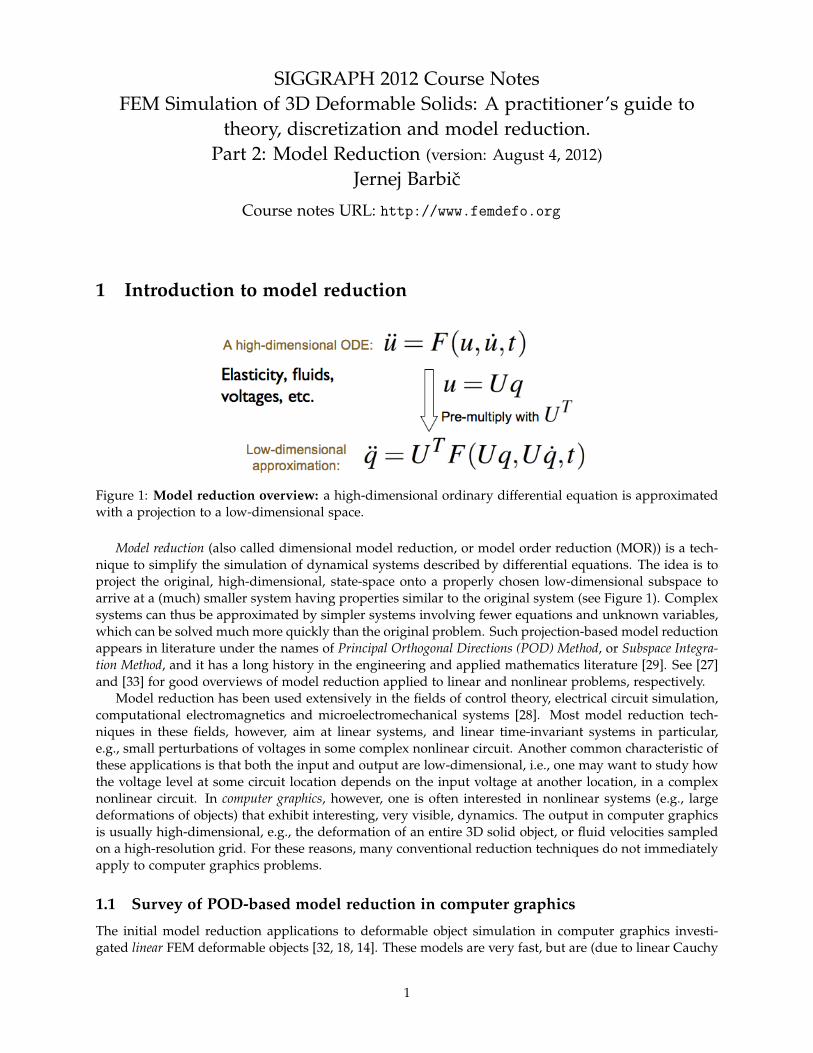
Figure 1: Model reduction overview: a high-dimensional ordinary differential equation is approximatedwith a projection to a low-dimensional space.

Model reduction (also called dimensional model reduction, or model order reduction (MOR)) is a tech-nique to simplify the simulation of dynamical systems described by differential equations. The idea is toproject the original, high-dimensional, state-space onto a properly chosen low-dimensional subspace toarrive at a (much) smaller system having properties similar to the original system (see Figure 1). Complexsystems can thus be approximated by simpler systems involving fewer equations and unknown variables,which can be solved much more quickly than the original problem. Such projection-based model reductionappears in literature under the names of Principal Orthogonal Directions (POD) Method, or Subspace Integra-tion Method, and it has a long history in the engineering and applied mathematics literature [29]. See [27]and [33] for good overviews of model reduction applied to linear and nonlinear problems, respectively.

Model reduction has been used extensively in the fields of control theory, electrical circuit simulation,computational electromagnetics and microelectromechanical systems [28]. Most model reduction tech-niques in these fields, however, aim at linear systems, and linear time-invariant systems in particular,e.g., small perturbations of voltages in some complex nonlinear circuit. Another common characteristic ofthese applications is that both the input and output are low-dimensional, i.e., one may want to study howthe voltage level at some circuit location depends on the input voltage at another location, in a complexnonlinear circuit. In computer graphics, however, one is often interested in nonlinear systems (e.g., largedeformations of objects) that exhibit interesting, very visible, dynamics. The output in computer graphicsis usually high-dimensional, e.g., the deformation of an entire 3D solid object, or fluid velocities sampledon a high-resolution grid. For these reasons, many conventional reduction techniques do not immediatelyapply to computer graphics problems.

1.1 Survey of POD-based model reduction in computer graphics

The initial model reduction applications to deformable object simulation in computer graphics investi-gated linear FEM deformable objects [32, 18, 14]. These models are very fast, but are (due to linear Cauchy

1

strain) accurate only for small deformations and produce visible artifacts under large deformations. Inorder to avoid such artifacts, it is necessary to apply reduction to nonlinear elasticity. For real-time geomet-rically nonlinear deformable objects (quadratic Green-Lagrange strain), such an approach was presentedby Barbic and James [6, 4], who also gave an automatic approach to select a quality low-dimensionalbasis, using modal derivatives. An and colleagues [2] demonstrated how to efficiently support arbitrarynonlinear material models. Model reduction has also been used for fast sound simulation [17, 10] and tosimulate frictional contact between deformable objects [21]. For deformable FEM offline simulations, Kimand James [23] applied online model reduction to adaptively replace expensive full simulation steps withreduced steps, which made it possible to throttle the simulation costs at run-time. Treuille and colleaguesapplied model reduction to fluid simulation in computer graphics [39]. Wicke and colleagues [41] im-proved Treuille’s fluid method to support reduced fluid simulations on several (inter-connected) domainswith specialized basis functions on each domain (domain decomposition for fluids). Recently, Barbic andZhao [8] demonstrated a domain decomposition method for open-loop solid deformable models, by em-ploying gradients of polar decomposition rotation matrices, whereas Kim and James [24] tackled a similarproblem using inter-domain spring forces.

2 Linear modal analysis

Figure 2: Linear modes for a cantilever beam.

Although elastic objects can in principle deform arbitrarily, they tend to have a bias in deforming intocertain characteristic, low-energy shapes. Most of us will remember the high-school physics example of astring stretched between two walls (or, say, a violin string), where one studies the natural frequencies ωiof the string, together with their associated shapes, typically of the form sin(ωix) and cos(ωix). The sameintuition carries over to arbitrary three-dimensional elastic objects deforming by a small amount aroundtheir rest configuration, whether it be a metal wire, a thin shell (e.g., cloth on a character), or a solid 3D tetmesh model of a skyscraper. The low-frequency modes are the deformations, which, for a given amountof displaced mass (or volume), subject to specific boundary conditions such as fixed vertices, increasethe elastic strain energy of the object by the least amount. In other words, they are the shapes with theleast resistance to deformation. How are the modes and frequencies computed? One has to first form thesystem mass and stiffness matrices M ∈ R3n×3n and K ∈ R3n×3n, where n is the number of mesh vertices.The specific approach to compute M and K depends on each particular mechanical system. For example,the tet skyscraper may be modeled using 3D FEM elasticity, whereas for a cloth model one may computeM by lumping the mass at the vertices, and set K to the gradient of the internal cloth forces (in the restconfiguration), computed, say, using the Baraff-Witkin cloth model [3]. Once M and K are known, one hasto prescribe boundary conditions, i.e., specify how the object is constrained. The modes and frequenciesgreatly depend on this choice. It is possible to set no boundary conditions, in which case one obtains free-flying modes. In order to compute the modes, one forms matrices M and K where the rows and columnscorresponding to the fixed degrees of freedom have been removed from M and K. Then, one solves thegeneralized eigenvalue problem

Kx = λMx. (1)

Matrices M and K are typically large and sparse. One can solve the eigenvalue problem, say, using theArnoldi iteration implemented by the ARPACK eigensolver [26]. This solver is free, and has performedvery well in various model reduction computer graphics projects by Jernej Barbic and other researchers inthe field. Because M and K are symmetric positive-definite (in typical applications, e.g., deformable object

2

in the rest configuration), the eigenvalues are real and non-negative. One seeks the smallest eigenvaluesλi and their associated eigenvectors ψi, i = 1, 2, . . . , k, where k is the number of modes to be retained.For objects with no constrained vertices (free-flying objects), the first six eigenvalues are zero and themodes correspond to rigid translations and infinitesimal rotations; these modes are typically discarded.The eigenvalues are squares of the natural frequencies of vibration, λi = ω2

i , and the eigenvectors ψi arethe modes. It should be noted that one typically inserts zeros into ψi at locations of fixed degrees offreedom, so that the resulting vector is of length 3n. In order to check that the eigensolver was successful,it is common to visualize the individual modes, by animating them as ψisin(ωit), where t is time. Thedifferent modal vectors are typically assembled into a linear modal basis matrix U = [ψ1, . . . , ψk] ∈ R3n×k.

2.1 Small deformation simulation using linear modal analysis

Small deformations u ∈ R3n (n is the number of mesh vertices) follow the equation

Mu + Du + Ku = f , (2)

where M, D, K ∈ R3n×3n are the mass, damping and stiffness matrices, respectively, and f ∈ R3n are theexternal forces [35]. Equation 2 is a linear, high-dimensional ordinary differential equation, obtained byapplying the Finite Element Method (FEM) to the linearized partial differential equations of elasticity. Itis most commonly applied to 3D solids, but can also model shells and strands. It is only accurate undersmall deformations; very visible artifacts appear under large deformations. Equation 2 models the objectat full resolution (no reduction), which means that it incorporates transient effects such as (localized)waves traveling across the object. It is often employed, for example, to perform earthquake simulation,typically using supercomputers on large meshes involving millions of degrees of freedom [1]. For real-time applications, the computational costs of timestepping Equation 2 may be prohibitive. Instead, onecan perform model reduction, by approximating the deformation vector u as u = Uz, where z ∈ Rk is avector of modal amplitudes (typically k 3n). If we choose damping to be a linear combination of M andK, D = αM + βK, for some scalars α, β > 0 (this is called Rayleigh damping), and pre-multiply Equation 2by UT , Equation 2 projects to k independent one-dimensional ordinary differential equations

zi + (α + βλi)zi + λizi = ψTi f , (3)

for i = 1, . . . , k. Here, we have used the fact that the modes are generalized eigenvectors Kψi = λi Mψi,and are therefore mass-orthonormal, (Mψi)Tψj = 0 when i 6= j, and (Mψi)Tψi = 1 for all i. The one-dimensional equations given in (3) can be timestepped independently. This can be done very efficiently(see, e.g., [18]). The full deformation can be reconstructed by multiplying u = Uz. This multiplicationis fast when k is small (a few hundred modes). It can also be performed very efficiently in graphicshardware [18]. It can be shown that as k → 3n, this approximation converges to the solution of Equation 2.This property is very useful, as it makes it possible to trade computation accuracy for speed.

2.2 Application to sound simulation

Sound originates from mechanical vibration of objects. These mechanical vibrations excite the surroundingmedium (typically air or water), and the pressure waves then propagate to the listener location. The objectmechanical vibrations are usually modeled using FEM and the equations of elasticity, whereas the pressurepropagation is usually modeled by the wave equation. There are varying degrees of approximation thatcan be applied to each of these two tasks. Because deformation amplitudes in sound applications aresmall, linear elasticity is often employed for their simulation [31, 17]. However, richer, nonlinear soundcan be produced using nonlinear simulation [10]. Linear simulation is straightforward and follows thematerial from Section 2.1. For each object that is to produce sound, one first has to set the fixed vertices(if any), and extract the modes. Next, one runs any physical simulation (typically rigid body simulation),producing contact forces. These forces are then used as external forces f for the modal oscillators inEquation 3, producing modal excitations zi(t). It remains to be described how zi(t) are used to generate

3

the sound signal s(t). A very common approach is to assign some meaningful weights wi to each mode,and compute sound as

s(t) =k

∑i=1

wizi(t), (4)

where k is the number of modes. The weights wi can be set to a constant, wi = 1 [31], or they can bemade non-constant to model the fact that different modes radiate with different intensities. Alternatively,weights can be made to depend on the listener location x, wi = wi(x, t), by solving the spatial part of thewave equation (Helmholtz equation) [17, 10]. Such spatially-dependent weights can model diffraction ofsound around the scene geometry.

3 Model reduction of nonlinear deformations

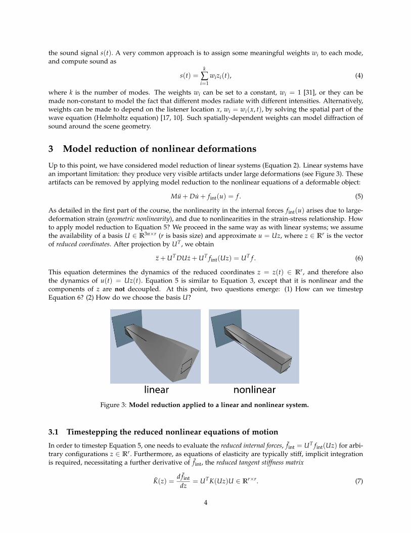
Up to this point, we have considered model reduction of linear systems (Equation 2). Linear systems havean important limitation: they produce very visible artifacts under large deformations (see Figure 3). Theseartifacts can be removed by applying model reduction to the nonlinear equations of a deformable object:

Mu + Du + fint(u) = f . (5)

As detailed in the first part of the course, the nonlinearity in the internal forces fint(u) arises due to large-deformation strain (geometric nonlinearity), and due to nonlinearities in the strain-stress relationship. Howto apply model reduction to Equation 5? We proceed in the same way as with linear systems; we assumethe availability of a basis U ∈ R3n×r (r is basis size) and approximate u = Uz, where z ∈ Rr is the vectorof reduced coordinates. After projection by UT , we obtain

z + UT DUz + UT fint(Uz) = UT f . (6)

This equation determines the dynamics of the reduced coordinates z = z(t) ∈ Rr, and therefore alsothe dynamics of u(t) = Uz(t). Equation 5 is similar to Equation 3, except that it is nonlinear and thecomponents of z are not decoupled. At this point, two questions emerge: (1) How can we timestepEquation 6? (2) How do we choose the basis U?

Figure 3: Model reduction applied to a linear and nonlinear system.

3.1 Timestepping the reduced nonlinear equations of motion

In order to timestep Equation 5, one needs to evaluate the reduced internal forces, fint = UT fint(Uz) for arbi-trary configurations z ∈ Rr. Furthermore, as equations of elasticity are typically stiff, implicit integrationis required, necessitating a further derivative of fint, the reduced tangent stiffness matrix

K(z) =d fint

dz= UTK(Uz)U ∈ Rr×r. (7)

4

Here K(u) = d fint/du is the (unreduced) tangent stiffness matrix in configuration u. Note that in general,the term fint cannot be algebraically simplified; its evaluation must proceed by first forming Uz, thenevaluating fint(Uz) and finally forming a projection by pre-multiplying with UT . Evaluation of K(z) iseven more complex. Once fint(z) and K(z) are known, one can use any implicit integrator to timestep thesystem (see [4] for details). The key important fact is that this integrator will need to solve a dense r× rlinear system as opposed to a sparse 3n× 3n system as is the case with implicit integration of unreducedsystems. Since r 3n, this usually leads to significant computational savings.

How to evaluate fint(z) and K(z) in practice? If the simulation is geometrically nonlinear, but materiallylinear, then it can be shown [4] that each component of fint(u) is a cubic polynomial in the components ofu [4]. Consequently, fint are cubic polynomials in the components of z. Note that this is a manifestation ofa more general principle: for any polynomial function G(u), its projection UTG(Uz) will be a polynomialin z, of the same degree. Treuille and colleagues, for example, exploited this fact with quadratic advectionforces for reduced fluids [39]. For geometrically nonlinear materials, one can precompute the coefficientsof the cubic polynomials. As there are r components of the reduced force, each of which is a cubicpolynomial in r variables, the necessary storage is O(r4). For moderate values of r (r < 30), this storageis manageable (under one megabyte; details are in [4]). Because the reduced stiffness matrix K(z) is thegradient of fint with respect to z, the reduced stiffness matrix is a quadratic function in z with coefficientsdirectly related to those of the reduced internal forces. For exact evaluation of internal forces and tangentstiffness matrices, all polynomial terms must be “touched” exactly once. Therefore, the cost of evaluationof reduced internal forces and tangent stiffness matrices is O(r4), whereas the cost of implicit integrationis O(r3).

For general materials, An and colleagues [2] have designed a fast approximation scheme which candecrease the reduced internal force and stiffness matrix computation time to O(r2) and O(r3), respectively.For simulations that use implicit integration, the runtime complexity is therefore O(r3). The method worksby observing that the elastic strain energy E(z) and internal forces fint(z), for reduced coordinates z, areobtained by integration of the energy density Ψ(X, z) and its gradient over the entire mesh:

E(z) =∫

ΩΨ(X, z)dV, (8)

fint(z) =∫

Ω

∂Ψ(X, z)∂z

dV. (9)

As opposed to evaluating fint using the exact formula fint = UT fint(Uz), An and colleagues approximatethe integral in (9) using numerical quadrature. In order to do so, they determine positions Xi ∈ Ω, andweights wi ∈ R, such that

fint(z) =∫

Ω

∂Ψ(X, z)∂z

dV ≈T

∑i=1

wi g(Xi, z), (10)

K(z) ≈T

∑i=1

wi∂g(Xi, z)

∂z, (11)

where g(X, z) = ∂Ψ(X, z)/∂z. At runtime, given a value z, one then only has to evaluate g(Xi, z) and∂g(Xi, z)/∂z, for i = 1, . . . , T and sum the terms together. The number of quadrature points T is usuallyset to T = r. Positions and weights are obtained using a training process. Given a set of representa-tive “training” reduced coordinates z(1), . . . , z(N), the method computes positions and weights that bestapproximate the reduced force fint for these training datapoints. To avoid overfitting and to keep thestiffness matrix symmetric positive-definite, the weights wi are chosen to be non-negative, using nonneg-ative least squares (NNLS) [25]. The positions Xi are determined using a greedy approach, designed tominimize the NNLS error residual (details in [2]).

5

3.2 Choice of basis

The matrix U is a time-invariant matrix specifying a basis of some r-dimensional (r 3n) linear subspaceof R3n. The basis is assumed to be mass-orthonormal, i.e., UT MU = I. If this is not the case, one caneasily convert U to such a basis using a mass-weighted Gramm-Schmidt process. For each fixed r > 1,there is an infinite number of possible choices for the linear subspace and for its basis. Good subspacesare low-dimensional spaces which well-approximate the space of typical nonlinear deformations. Thechoice of subspace depends on geometry, boundary conditions and material properties. Selection of agood subspace is a non-trivial problem. We now present two choices: basis from simulation data (“PODbasis”), and basis from modal derivatives. The former requires pre-simulation (using a general deformablesolver), whereas the latter can create a basis automatically without pre-simulation.

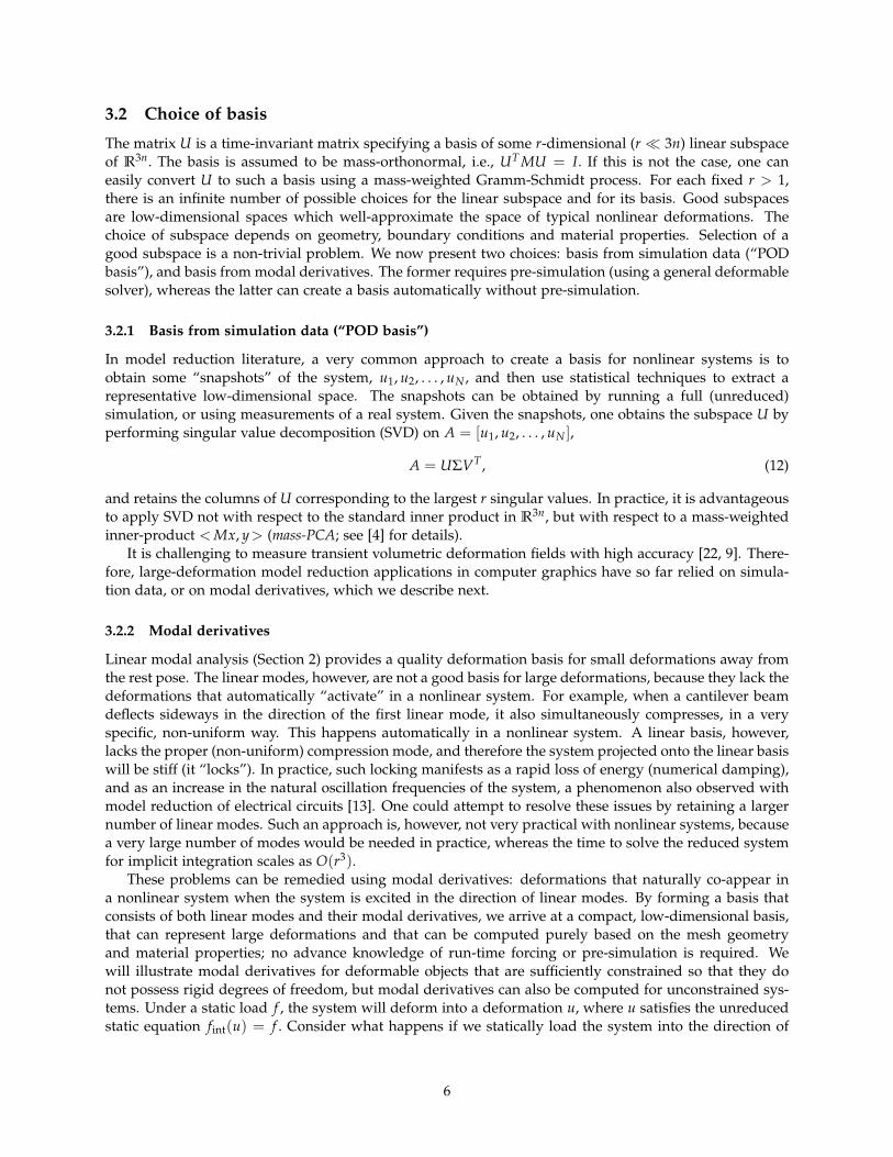
3.2.1 Basis from simulation data (“POD basis”)

In model reduction literature, a very common approach to create a basis for nonlinear systems is toobtain some “snapshots” of the system, u1, u2, . . . , uN , and then use statistical techniques to extract arepresentative low-dimensional space. The snapshots can be obtained by running a full (unreduced)simulation, or using measurements of a real system. Given the snapshots, one obtains the subspace U byperforming singular value decomposition (SVD) on A = [u1, u2, . . . , uN ],

A = UΣVT , (12)

and retains the columns of U corresponding to the largest r singular values. In practice, it is advantageousto apply SVD not with respect to the standard inner product in R3n, but with respect to a mass-weightedinner-product < Mx, y> (mass-PCA; see [4] for details).

It is challenging to measure transient volumetric deformation fields with high accuracy [22, 9]. There-fore, large-deformation model reduction applications in computer graphics have so far relied on simula-tion data, or on modal derivatives, which we describe next.

3.2.2 Modal derivatives

Linear modal analysis (Section 2) provides a quality deformation basis for small deformations away fromthe rest pose. The linear modes, however, are not a good basis for large deformations, because they lack thedeformations that automatically “activate” in a nonlinear system. For example, when a cantilever beamdeflects sideways in the direction of the first linear mode, it also simultaneously compresses, in a veryspecific, non-uniform way. This happens automatically in a nonlinear system. A linear basis, however,lacks the proper (non-uniform) compression mode, and therefore the system projected onto the linear basiswill be stiff (it “locks”). In practice, such locking manifests as a rapid loss of energy (numerical damping),and as an increase in the natural oscillation frequencies of the system, a phenomenon also observed withmodel reduction of electrical circuits [13]. One could attempt to resolve these issues by retaining a largernumber of linear modes. Such an approach is, however, not very practical with nonlinear systems, becausea very large number of modes would be needed in practice, whereas the time to solve the reduced systemfor implicit integration scales as O(r3).

These problems can be remedied using modal derivatives: deformations that naturally co-appear ina nonlinear system when the system is excited in the direction of linear modes. By forming a basis thatconsists of both linear modes and their modal derivatives, we arrive at a compact, low-dimensional basis,that can represent large deformations and that can be computed purely based on the mesh geometryand material properties; no advance knowledge of run-time forcing or pre-simulation is required. Wewill illustrate modal derivatives for deformable objects that are sufficiently constrained so that they donot possess rigid degrees of freedom, but modal derivatives can also be computed for unconstrained sys-tems. Under a static load f , the system will deform into a deformation u, where u satisfies the unreducedstatic equation fint(u) = f . Consider what happens if we statically load the system into the direction of

6

Figure 4: Modal derivatives for a cantilever beam.

linear modes. In particular, suppose we apply a static force load MUlinΛp, where M is the mass ma-trix, Ulin = [ψ1, ψ2, . . . , ψk] is the linear modal matrix, Λ is the diagonal matrix of squared frequenciesdiag(ω2

1, . . . , ω2k), and p ∈ Rk is some parameter that controls the strength of each mode in the load.

It can be easily verified that these are the force loads which, for small deformations, produce deforma-tions within the space spanned by the linear modes. Given a p, we can solve the nonlinear equationfint(u) = MUlinΛp for u, i.e., we can define a unique function u = u(p) (mapping from Rk to R3n, andC∞ differentiable), such that

fint(u(p)) = MUlinΛp, (13)

for every p ∈ Rk in some sufficiently small neighborhood of the origin in Rk. Can we compute the Taylorseries expansion of u in terms of p? By differentiating Equation 13 with respect to p, one obtains

∂ fint

∂u∂u∂p

= MUlinΛ, (14)

which is valid for all p in some small neighborhood of the origin of Rk. In particular, for p = 0k, we getK ∂u

∂p = MUlinΛ. Therefore, ∂u∂p = Ulin, i.e., the first-order response of the system are the linear modes, as

expected. To compute the second order derivatives of u, we differentiate Equation 14 one order further byp, which, when we set p = 0k, gives us

K∂2u

∂pi∂pj= −(H : ψj)ψi. (15)

Here, H is the Hessian stiffness tensor, the first derivative of the tangent stiffness matrix, evaluated at u = 0(see [4]). The deformation vectors

Φij =∂2u

∂pi∂pj(16)

are called modal derivatives. They are symmetric, Φij = Φji, and can be computed from Equation 15 bysolving linear systems with a constant matrix K (stiffness matrix of the origin). Because K is constant andsymmetric positive-definite, it can be pre-factored using Cholesky factorization. One can then rapidly (inparallel if desired) compute all the modal derivatives, 0 ≤ i ≤ j < k. Note that the modal derivatives are,by definition, the second derivatives of u = u(p). The second-order Taylor series expansion is therefore

u(p) =k

∑i=1

Ψi pi +12

k

∑i=1

k

∑j=1

Φij pi pj + O(p3). (17)

7

Figure 5: Extreme shapes captured by modal derivatives: Although modal derivative are computedabout the rest pose, their deformation subspace contains sufficient nonlinear content to describe largedeformations. Left: Spoon (k = 6, r = 15) is constrained at far end. Right: Beam (r = 5, twist angle=270)is simulated in a subspace spanned by “twist” linear modes and their derivatives Ψ4, Ψ9, Φ44, Φ49, Φ99.

The modal derivatives, together with the linear modes, therefore span the natural second-order systemresponse for large deformations around the origin.

Creating the basis U: Equation 17 suggests that the linear space spanned by all vectors Ψi and Φij

is a natural candidate for a basis (after mass-Gramm-Schmidt mass-orthonormalization). However, itsdimension k + k(k + 1)/2 may be prohibitive for real-time systems. In practice, we obtain a smaller basisby scaling the modes and derivatives according to the eigenvalues of the corresponding linear modes, andapplying mass-PCA on the “dataset”

λ1

λjΨj | j = 1, . . . , k

∪

λ21

λiλjΦij | i ≤ j; i, j = 1, . . . , k

. (18)

The scaling puts greater weight on dominant low-frequency modes and their derivatives, which couldotherwise be masked by high-frequency modes and derivatives.

Figure 6: Reduced simulations: Left: Model reduction enables interactive simulations of nonlinear de-formable models. Right: reduction also enables fast large-scale multibody dynamics simulations, withnonlinear deformable objects undergoing free flight motion. Collisions among the 512 baskets were re-solved using BD-Trees [20].

8

4 Model reduction and domain decomposition

Model reduction as described in the previous section is global: it reduces the entire object using a sin-gle, global basis. Unless r is large, it is difficult to capture local detail using such a basis. Because thecomputation time grows at least as O(r3) (time to solve the dense r × r system [2]), large values of r(several hundreds of modes) are not practical. It is therefore natural to ask if the object can somehow bedecomposed into smaller pieces, each of which is reduced separately, and the pieces are then connectedinto a global system. This is the idea of domain decomposition, a classical technique in applied mathe-matics and engineering. In engineering applications, however, the deformations are typically small. Incomputer graphics, we have to accommodate large deformations (e.g., rotations) in the interfaces joiningtwo domains, which means that standard domain decomposition techniques cannot simply be extendedto computer graphics problems.

In computer graphics, domain decomposition for deformable models has initially been applied to smalldomain deformations and with running times dependent on the number of domain and interface vertices.For example, a linear quasi-static application using Green’s functions has been presented in [19], whereasHuang and colleagues [15] exploited redundancy in stiffness matrix inverses to combine linear FEM withdomain decomposition. Recently, domain decomposition under large deformations has received signifi-cant attention in computer graphics literature. Barbic and Zhao [8] demonstrated a domain decompositionmethod by employing gradients of polar decomposition rotation matrices, whereas Kim and James [24]tackled a similar problem using inter-domain spring forces.

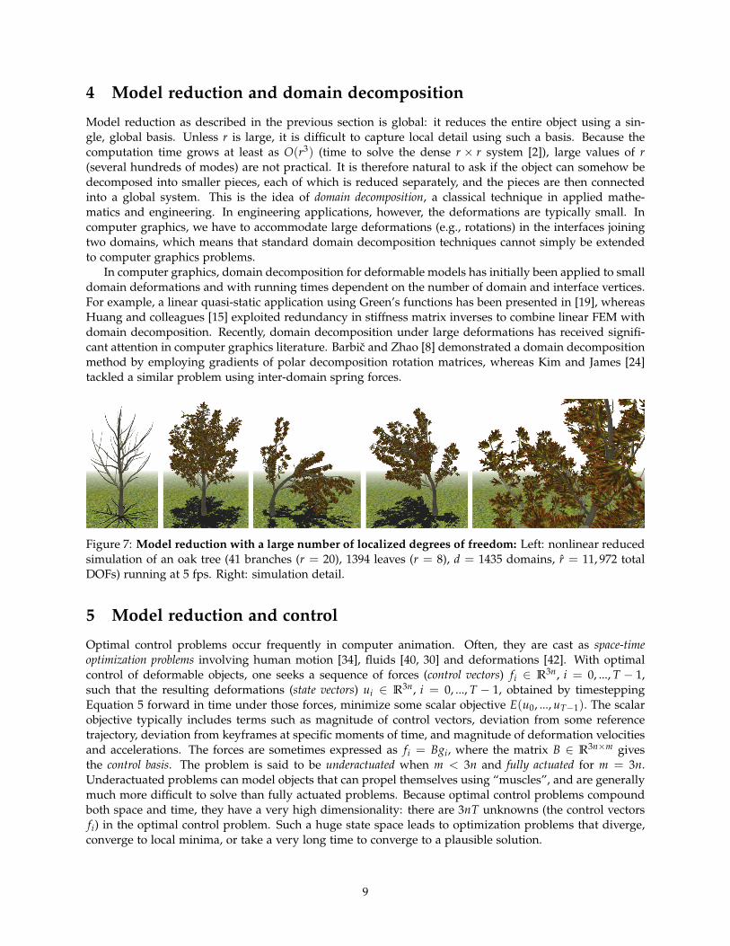
Figure 7: Model reduction with a large number of localized degrees of freedom: Left: nonlinear reducedsimulation of an oak tree (41 branches (r = 20), 1394 leaves (r = 8), d = 1435 domains, r = 11, 972 totalDOFs) running at 5 fps. Right: simulation detail.

5 Model reduction and control

Optimal control problems occur frequently in computer animation. Often, they are cast as space-timeoptimization problems involving human motion [34], fluids [40, 30] and deformations [42]. With optimalcontrol of deformable objects, one seeks a sequence of forces (control vectors) fi ∈ R3n, i = 0, ..., T − 1,such that the resulting deformations (state vectors) ui ∈ R3n, i = 0, ..., T − 1, obtained by timesteppingEquation 5 forward in time under those forces, minimize some scalar objective E(u0, ..., uT−1). The scalarobjective typically includes terms such as magnitude of control vectors, deviation from some referencetrajectory, deviation from keyframes at specific moments of time, and magnitude of deformation velocitiesand accelerations. The forces are sometimes expressed as fi = Bgi, where the matrix B ∈ R3n×m givesthe control basis. The problem is said to be underactuated when m < 3n and fully actuated for m = 3n.Underactuated problems can model objects that can propel themselves using “muscles”, and are generallymuch more difficult to solve than fully actuated problems. Because optimal control problems compoundboth space and time, they have a very high dimensionality: there are 3nT unknowns (the control vectorsfi) in the optimal control problem. Such a huge state space leads to optimization problems that diverge,converge to local minima, or take a very long time to converge to a plausible solution.

9

Figure 8: Fast authoring of animations with dynamics [5]: This soft-body dinosaur sequence consistsof five walking steps, and includes dynamic deformation effects due to inertia and impact forces. Eachstep was generated by solving a space-time optimization problem, involving 3 user-provided keyframes,and requiring only 3 minutes total to solve due to a proper application of model reduction to the controlproblem. Unreduced optimization took 1 hour for each step. The four images show output poses at timescorresponding to four consecutive keyframes (out of 11 total). For comparison, the keyframe is shown inthe top-left of each image.

Model reduction is very beneficial to optimal control because it greatly reduces the state and controlsize. The states ui are replaced with the reduced states zi, the control vectors fi are replaced with thereduced internal forces fi, and Equation 5 is replaced with its reduced version (Equation 6). Althoughsuch a reduced optimal control problem only approximates the original problem, its dimensionality isonly rT 3nT; therefore, the occurrence of local minima is greatly decreased. Optimal reduced forcescan be found faster than unreduced forces, because one can rapidly explore the solution space by runningmany reduced forward simulations and by quickly evaluating the reduced objective gradient [5] (Figure 8).Standard controllers such as the linear-quadratic regulator [37] are impractical with deformable objects asthey involve dense 3n × 3n gain matrices. With reduction, however, such control becomes feasible asthe gain matrices are now much smaller (r× r). Barbic and Popovic [7] exploited such a combination ofLQR control and model reduction for real-time tracking of nonlinear deformable object simulations, usingminimal (“gentle”) forces.

6 Free software for model reduction

The implementation of [6] (by Jernej Barbic) is freely available on the web (BSD license) at:http://www.jernejbarbic.com/code. It includes

1. a precomputation utility to compute linear modes (Equation 1) and modal derivatives (Equation 15),and to construct the simulation basis U (mass-PCA applied to the dataset of Equation 18); optionally,the basis can also be computed from pre-existing simulation data (“POD basis”),

2. a precomputation utility to compute the cubic polynomial coefficients for reduced internal forcesfint and stiffness matrices K (Section 3.1), for isotropic geometrically nonlinear material model (St.Venant-Kirchhoff material)

3. an efficient C/C++ library to timestep the reduced model precomputed in the above steps 1., 2.(Equation 6), and an example run-time driver.

The code shares basic classes with Vega, a general-purpose simulator for FEM nonlinear 3D deformableobjects (including deformable dynamics), also available at the same URL (BSD license).

10

Figure 9: Precomputation utility to compute linear modes, derivatives, basis for large deformations, andcubic polynomial coefficients. Freely available (BSD license) at http://www.jernejbarbic.com/code .

7 Deformation warping

As outlined in Section 3, linear modal analysis (Section 2) leads to visible artifacts under large defor-mations, and these artifacts can be removed by applying model reduction to the nonlinear equations ofmotion. Deformation warping is an alternative, purely geometric, approach to remedy the same problem.The idea is to keep Equation 2 as the underlying dynamic equation, but to post-process the resultingdeformations u using a geometric “filter” that removes large-deformation artifacts. For example, givena tetrahedral mesh, warping establishes a mapping that maps linearized deformations u ∈ R3n (awayfrom the rest configuration) to “good-looking” large deformations q = W(u) ∈ R3n (also away from therest configuration). The user is only shown the corrected deformations q. Warping is very robust. Forexample, twisting deformations, with local rotations as large as several complete 360 degrees cycles, canbe easily accommodated. The underlying dynamics, however, is still linear, and this is visible with large-deformation motion as linear deformations essentially follow a sinusoidal curve, sin(ωit). In contrast,objects simulated using nonlinear methods usually stiffen under large deformations, and therefore spenda smaller percentage of the oscillation cycle time at large deformations.

The idea that modes could be warped to correct large deformation artifacts was first observed byChoi and Ko [11]. They noticed that, by taking the curl of each modal vector, one can derive per-vertexinfinitesimal rotations due to the activation of each mode. These rotations can then be integrated in time,resulting in large deformations free of artifacts. Although not surveyed here in detail, their approach isfast, and laid the foundation for other warping methods developed later.

7.1 Rotation-strain coordinate warping

In these notes, we describe a recent efficient flavor of warping, the rotation-strain coordinate warping [16]. LetGj ∈ R9×3n be the discrete gradient operator of tet j, i.e., deformation gradient of tet j under deformationu ∈ R3n equals I + Gju. Decompose the 3× 3 matrix Gju into a symmetric and antisymmetric component,

Gju =Gju + (Gju)T

2+

Gju− (Gju)T

2. (19)

We can then denote the upper triangle of the symmetric part as εj ∈ R6, and the skew-vector correspond-ing to the antisymmetric part as ωj ∈ R3. We then assemble [εj, ωj] for all tets into a vector y(u) ∈ R9#tets;

11

Figure 10: Warping corrects linearization artifacts under large deformations.

denote yε,j = εj and yω,j = ωj. Vector y forms the rotation-strain coordinates of the mesh. Given a linearizeddeformation u, we then postulate that we should seek a deformation q so that the deformation gradientinside tet j equals

exp(yω,j

)(I + sym(yε,j)

). (20)

Here, sym(x) is the 3× 3 symmetric matrix corresponding to its upper-triangle x ∈ R6, x is the 3× 3skew-symmetric cross-product matrix corresponding to vector x ∈ R3 (xv = x× v for all v ∈ R3), and expis the matrix exponential function [36]. This condition cannot be satisfied for all the tets simultaneously.Instead, given u, we find a deformation q under which the deformation gradients are as close as possibleto those given by Equation 20. This can be done by solving the following least-squares problem:

arg minq

#tets

∑j=1

Vj||I + Gjq− exp(yω,j

)(I + sym(yε,j)

)||2F, (21)

subject to pinned vertices (22)

where || ||F denotes the Frobenius norm of a 3× 3 matrix, and Vj is the volume of tet j. The pinned verticesare the vertices where the model is rooted to the ground (boundary conditions). For free-flying objects, aconstraint can be formed that keeps the center of mass unmodified. The objective function in Equation 21is quadratic in q, and can be rewritten as

||VGq− b||22, (23)

for V = diag(√

V1,√

V1, . . . ,√

V#tets) (each entry repeated 9x), and where G ∈ R9#tets×3n is the gradientmatrix assembled from all Gj. The nine-block of vector b ∈ R9#tets corresponding to tet j, expressed as arow-major 3× 3 matrix, equals

bj =√

Vj(exp(yω,j)(I + sym(yε,j))− I

). (24)

In a typical tet mesh, there are more tets than vertices, therefore, the optimization problem is overcon-strained. The minimization can be performed via Lagrange multipliers, by solving[

L ddT 0

] [qλ

]=

[(VG)Tb

0

], (25)

where L = GTV2G, and where d corresponds to the pinned input vertices (note: an implementation cansimply remove the rows-columns from L; this is equivalent). Matrix L is called the discrete Laplacian of themesh. It only depends on the input mesh geometry, and not on U or u. The system matrix in Equation 25is sparse and constant, and can be pre-factored, so warping can be performed efficiently at runtime.

12

7.2 Warping for triangle meshes

Triangle meshes are commonly employed in computer graphics, say, for simulation of thin shells andcloth. Such physical systems also produce the mass matrix M and stiffness matrix K. Therefore, the smalldeformation analysis (Equation 2) and model reduction (as in Equation 3) apply also to such problems. Inorder to apply warping, however, we must define deformation gradients for each triangle. As observedby Sumner and Popovic [38], the three vertices of a triangle before and after deformation do not fullydetermine the affine transformation since they do not establish how the space perpendicular to the triangledeforms. They resolve this issue by adding a (fictitious) fourth vertex v4,

v4 = v1 +(v2 − v1)× (v3 − v1)√|(v2 − v1)× (v3 − v1)|

, (26)

where v1, v2, v3 are the triangle vertices. Vertices v1, v2, v3, v4 define a tetrahedron. Let v′1, v′2, v′3 denotethe deformed vertex positions; then, we can use (26) to compute the deformed fictitious vertex v′4. Thedeformation gradient F for the triangle equals

F =

v′2 − v′1 v′3 − v′1 v′4 − v′1

v2 − v1 v3 − v1 v4 − v1

−1

. (27)

Given the deformation gradient, warping then proceeds in the same way as described for tetrahedralmeshes in previous sections. A more principled version of triangle mesh warping has been presentedby [12].

8 Acknowledgements

This work was sponsored by the National Science Foundation (CAREER-53-4509-6600). I would like tothank Eftychios Sifakis and Yili Zhao for helpful suggestions.

References

[1] V. Akcelik, J. Bielak, G. Biros, I. Epanomeritakis, A. Fernandez, O. Ghattas, E. J. Kim, J. Lopez,D. O’Hallaron, T. Tu, and J. Urbanic. High-resolution forward and inverse earthquake modeling onterascale computers. In Proceedings of ACM/IEEE SC2003, 2003.

[2] S. S. An, T. Kim, and D. L. James. Optimizing cubature for efficient integration of subspace deforma-tions. ACM Trans. on Graphics, 27(5):165:1–165:10, 2008.

[3] D. Baraff and A. P. Witkin. Large Steps in Cloth Simulation. In Proc. of ACM SIGGRAPH 98, pages43–54, July 1998.

[4] J. Barbic. Real-time Reduced Large-Deformation Models and Distributed Contact for Computer Graphics andHaptics. PhD thesis, Carnegie Mellon University, Aug. 2007.

[5] J. Barbic, M. da Silva, and J. Popovic. Deformable object animation using reduced optimal control.ACM Trans. on Graphics (SIGGRAPH 2009), 28(3):53:1–53:9, 2009.

[6] J. Barbic and D. L. James. Real-time subspace integration for St. Venant-Kirchhoff deformable models.ACM Trans. on Graphics, 24(3):982–990, 2005.

[7] J. Barbic and J. Popovic. Real-time control of physically based simulations using gentle forces. ACMTrans. on Graphics (SIGGRAPH Asia 2008), 27(5):163:1–163:10, 2008.

13

[8] J. Barbic and Y. Zhao. Real-time large-deformation substructuring. ACM Trans. on Graphics (SIG-GRAPH 2011), 30(4):91:1–91:7, 2011.

[9] B. Bickel, M. Baecher, M. Otaduy, W. Matusik, H. Pfister, and M. Gross. Capture and modeling ofnon-linear heterogeneous soft tissue. ACM Trans. on Graphics (SIGGRAPH 2009), 28(3):89:1–89:9, 2009.

[10] J. N. Chadwick, S. S. An, and D. L. James. Harmonic Shells: A practical nonlinear sound model fornear-rigid thin shells. ACM Transactions on Graphics, 28(5):1–10, 2009.

[11] M. G. Choi and H.-S. Ko. Modal Warping: Real-Time Simulation of Large Rotational Deformationand Manipulation. IEEE Trans. on Vis. and Comp. Graphics, 11(1):91–101, 2005.

[12] M. G. Choi, S. Y. Woo, and H.-S. Ko. Real-Time Simulation of Thin Shells. Eurographics 2007, pages349–354, 2007.

[13] L. Daniel. Private correspondence with Prof. Luca Daniel, MIT.

[14] K. K. Hauser, C. Shen, and J. F. O’Brien. Interactive deformation using modal analysis with con-straints. In Proc. of Graphics Interface, pages 247–256, 2003.

[15] J. Huang, X. Liu, H. Bao, B. Guo, and H.-Y. Shum. An efficient large deformation method usingdomain decomposition. Computers & Graphics, 30(6):927 – 935, 2006.

[16] J. Huang, Y. Tong, K. Zhou, H. Bao, and M. Desbrun. Interactive shape interpolation through control-lable dynamic deformation. IEEE Trans. on Visualization and Computer Graphics, 17(7):983–992, 2011.

[17] D. L. James, J. Barbic, and D. K. Pai. Precomputed acoustic transfer: Output-sensitive, accurate soundgeneration for geometrically complex vibration sources. ACM Transactions on Graphics (SIGGRAPH2006), 25(3), 2006.

[18] D. L. James and D. K. Pai. DyRT: Dynamic Response Textures for Real Time Deformation SimulationWith Graphics Hardware. ACM Trans. on Graphics, 21(3):582–585, 2002.

[19] D. L. James and D. K. Pai. Real Time Simulation of Multizone Elastokinematic Models. In IEEE Int.Conf. on Robotics and Automation, pages 927–932, 2002.

[20] D. L. James and D. K. Pai. BD-Tree: Output-Sensitive Collision Detection for Reduced DeformableModels. ACM Trans. on Graphics, 23(3):393–398, 2004.

[21] D. M. Kaufman, S. Sueda, D. L. James, and D. K. Pai. Staggered Projections for Frictional Contact inMultibody Systems. ACM Transactions on Graphics, 27(5):164:1–164:11, 2008.

[22] A. E. Kerdok, S. M. Cotin, M. P. Ottensmeyer, A. M. Galea, R. D. Howe, and S. L. Dawson. Truthcube: Establishing physical standards for soft tissue simulation. Medical Image Analysis, 7(3):283–291,2003.

[23] T. Kim and D. James. Skipping steps in deformable simulation with online model reduction. ACMTrans. on Graphics (SIGGRAPH Asia 2009), 28(5):123:1–123:9, 2009.

[24] T. Kim and D. James. Physics-based character skinning using multi-domain subspace deformations.In Symp. on Computer Animation (SCA), pages 63–72, 2011.

[25] C. L. Lawson and R. J. Hanson. Solving Least Square Problems. Prentice Hall, Englewood Cliffs, NJ,1974.

[26] R. Lehoucq, D. Sorensen, and C. Yang. ARPACK Users’ Guide: Solution of large scale eigenvalueproblems with implicitly restarted Arnoldi methods. Technical report, Comp. and Applied Mathe-matics, Rice Univ., 1997.

14

[27] J.-R. Li. Model Reduction of Large Linear Systems via Low Rank System Gramians. PhD thesis, Mas-sachusetts Institute of Technology, 2000.

[28] R.-C. Li and Z. Bai. Structure preserving model reduction using a Krylov subspace projection formu-lation. Comm. Math. Sci., 3(2):179–199, 2005.

[29] J. L. Lumley. The structure of inhomogeneous turbulence. In A.M.Yaglom and V.I.Tatarski, editors,Atmospheric turbulence and wave propagation, pages 166–178, 1967.

[30] A. McNamara, A. Treuille, Z. Popovic, and J. Stam. Fluid control using the adjoint method. ACMTrans. on Graphics (SIGGRAPH 2004), 23(3):449–456, 2004.

[31] J. F. O’Brien, C. Shen, and C. M. Gatchalian. Synthesizing sounds from rigid-body simulations. InSymp. on Computer Animation (SCA), pages 175–181, 2002.

[32] A. Pentland and J. Williams. Good vibrations: Modal dynamics for graphics and animation. ComputerGraphics (Proc. of ACM SIGGRAPH 89), 23(3):215–222, 1989.

[33] M. Rewienski. A Trajectory Piecewise-Linear Approach to Model Order Reduction of Nonlinear DynamicalSystems. PhD thesis, Massachusetts Institute of Technology, 2003.

[34] A. Safonova, J. Hodgins, and N. Pollard. Synthesizing physically realistic human motion in low-dimensional, behavior-specific spaces. ACM Trans. on Graphics (SIGGRAPH 2004), 23(3):514–521, 2004.

[35] A. A. Shabana. Theory of Vibration, Volume II: Discrete and Continuous Systems. Springer–Verlag, NewYork, NY, 1990.

[36] R. B. Sidje. Expokit: A Software Package for Computing Matrix Exponentials. ACM Trans. on Mathe-matical Software, 24(1):130–156, 1998. www.expokit.org.

[37] R. F. Stengel. Optimal Control and Estimation. Dover Publications, New York, 1994.

[38] R. Sumner and J. Popovic. Deformation transfer for triangle meshes. ACM Trans. on Graphics (SIG-GRAPH 2004), 23(3):399–405, 2004.

[39] A. Treuille, A. Lewis, and Z. Popovic. Model reduction for real-time fluids. ACM Trans. on Graphics,25(3):826–834, 2006.

[40] A. Treuille, A. McNamara, Z. Popovic, and J. Stam. Keyframe control of smoke simulations. ACMTrans. on Graphics (SIGGRAPH 2003), 22(3):716–723, 2003.

[41] M. Wicke, M. Stanton, and A. Treuille. Modular bases for fluid dynamics. ACM Trans. on Graphics,28(3):39:1–39:8, 2009.

[42] C. Wojtan, P. J. Mucha, and G. Turk. Keyframe control of complex particle systems using the adjointmethod. In Symp. on Computer Animation (SCA), pages 15–23, Sept. 2006.

15