Signal and Information Processing (EEMCS, TU Delft)

Signal Processing Techniques to optimize the Detection of Radio Pulsar Signals

Daniel Hernando Portero

Supervisors Specialisation Type of report Date

Dr. Ir. Richard Heusdens Dr. Nikolay D. Gaubitch Signal Processing Master Of Science Thesis August 28, 2014

Signal Processing techniques to optimize the

detection of Radio Pulsar Signals

Master Of Science Thesis

For the degree of Master of Science in Telecommunications Engineeringat Polytechnic University of Catalonia under the Erasmus exchange

programme at Delft University of Technology

Faculty of Electrical Engineering, Mathematics and Computer Science (EEMCS)Delft University of Technology

Escola Tecnica Superior d’Enginyeria de Telecomunicacions de Barcelona (ETSETB)Polytechnic University of Catalonia

Daniel Hernando Portero

August 22, 2014

Cover Image: Four antennas of the Atacama Large Millimeter/submillimeter Array(ALMA) gaze up at the star-filled night sky, in anticipation of the work that lies ahead.The Moon lights the scene on the right, while the band of the Milky Way stretches acrossthe upper left.

Polytechnic University of CataloniaEscola Tecnica Superior d’Enginyeria de Telecomunicacions de BarcelonaSupervisor:Gregori Vazquez

Delft University of TechnologyIntelligent SystemsDepartmentMultimedia and Signal Processing (MSP) GroupSignal and Information Processing (SIP) LabSupervisors:Dr. Ir. Richard HeusdensDr. Nikolay D. Gaubitch

Copyright 2014 TU Delft, UPNAAll rights reserved.

Abstract

Key Words: ENR: Energy to Noise Ratio, GENR: Generalised Energy to Noise Ratio,TOA= Time of Arrival, Additive White Gaussian Noise, Antenna, De-Dispersion.

Radio Pulsars are neutron stars that emits high polarized electromagnetic pulses witha very accurate and stable periodicity. Adding the fact that those pulses have a widebandnature, so they can be received almost everywhere, make Radio Pulsar signals a perfectcandidate for navigation systems. The challenge, however, is that the Radio Pulsar signal isdegraded and submerged in Additive White Gaussian Noise when it is propagated throughthe ISM, so that make them difficult to detect.

The aim of the project is the design of the optimum receptor in order to estimate thetime of arrival of the Radio Pulsar Signal and make possible the real-time navigation. In thiscontribution I introduce the detection theory applied to radio pulsars and show the differentsignal processing techniques to improve the detection with the minimum computational timepossible. Although the previous work has centred in the Signal to Noise Ratio of the pulsarsignals, our focus will be the improvement of the Energy to Noise Ratio. We will see asEpoch Folding and the increment of the Bandwidth of the receiver are the best solutions.Moreover, Integration in Time appears to be one of the most promising techniques to simplifythe computation of the whole process. Also I demonstrate how the detection performance isnot affected by any digital or analogue filter, so Low-Pass Filtering will not have any effectin the receptor but to eliminate spurious signals. Some experiments with simulated wide-band signals are shown in order to prove the optimality of the signal processing techniques.Finally, summarizing all the results obtained in the Thesis, I propose two optimum receptorsfor pulsar-based navigation system applications.

It is known that the interstellar medium has a frequency dependent transfer character-istic, so the higher frequencies of a signal arrive earlier than the lower frequencies. Thiswill cause the pulse profile of the radio pulsar signal to appear dispersed in time. Up un-til now, the researchers have been performing de-dispersion techniques in order to obtainthe original power pulsar profile spending more than the 80% of the actual processing time.The prove to avoid de-dispersion without decreasing the detection performance are presented.

Furthermore, some simulations with data from the pulsar PSR B0329+54 recorded bythe Westerbork Observatory are shown. PSR B0329+54 is one of the strongest pulsar signalvisible in the northern hemisphere with one of the lowest Dispersion Measure, so it will beeasier to perform the Signal Processing techniques and see the profile of the pulse. We willsee how the results are not the ones expected, because the Radio pulsar signal happens to bevery Narrowband. Finally, I am going to give a possible explanation of what is happeningand in what part of the acquisition the wideband nature of the rotating star pulses are lost.

Acknowledgements

Writing the Acknowledgement of my Master Thesis means that I am finishing my studies.I still do not realize the importance of that fact, that in a brief period of time I will haveto face the first days of the rest of my life. I should feel scared, or doubtful with the thingsthat await me in the future, but truth be told I am eager to start and create my own path.

First of all I would like to thank Dr. Richard Heusdens for giving me the opportunityof working in that project with him. I have enjoyed all the moments of my research, eventhe hard ones. I have learned how to work alone and at the same time, being part of agroup. I also want to thank him for let me being part of the weekly discussions about theproject, where at the beginning I was a little bit lost but with the help of him and Dr.Nikolay Gaubitch I became one of them. I also want to express my gratitude to Dr. NikolayGaubitch for the good advices given during all my Thesis.

Several people have contributed to make this semester an unforgettable one. I would liketo start with the people from the Library Group. Although the first month we did not knoweach other, at the end we became a family. Of course I am talking about Roger, Paula,Benedetta, Cristina, Mikel, Pati and Riccardo. I hope we see each other soon. The secondgroup of people are the Marcushof/Roland crew. It will be difficult to forget all the dinners,beers, conversations we have shared. At the end I do not want to forget the rest of theInternational Group that has contributed to the most amazing period of my life. In special,many thanks to Roger, my library mate and best friend in that Erasmus that has helped meto being constant in that long-distance race that is the Thesis.

I will not end this Acknowledgements without saying thanks to my group of friends ofBarcelona. Although we have not seen each other for 6 month, our friendship is so strong thatthe distance has not had any effect on us. I am referring to Xavi, Cesc, Julia, Carles, Gonzalo,Pablo, David, Pedro and Anna. Also I want to give special thanks to David, Pedro and Xavifor giving me advices whenever I needed and to Anna for always being there no matter what.

Finally, I need to thank my parents, my sister, and the rest of my family, the most im-portant people of my life. It is only thanks to them that I have managed to become theperson I am today, for which I will be eternally grateful.

Delft, The NetherlandsDelft University of technology Daniel Hernando PorteroAugust 28, 2013

Table Of Contents

1 Introduction 11.1 Introduction to the Thesis . . . . . . . . . . . . . . . . . . . . . . . . . . . . . 11.2 Motivations . . . . . . . . . . . . . . . . . . . . . . . . . . . . . . . . . . . . . 11.3 Thesis goals . . . . . . . . . . . . . . . . . . . . . . . . . . . . . . . . . . . . . 11.4 Thesis contributions . . . . . . . . . . . . . . . . . . . . . . . . . . . . . . . . 21.5 Outline . . . . . . . . . . . . . . . . . . . . . . . . . . . . . . . . . . . . . . . 2

2 Radio Pulsar Signals 42.1 Pulsar description and emission properties . . . . . . . . . . . . . . . . . . . . 4

2.1.1 Pulsars . . . . . . . . . . . . . . . . . . . . . . . . . . . . . . . . . . . 42.1.2 Radio Pulsar signal characteristics . . . . . . . . . . . . . . . . . . . . 6

2.2 Propagation effects . . . . . . . . . . . . . . . . . . . . . . . . . . . . . . . . . 82.3 Pulsar-Based Navigation System . . . . . . . . . . . . . . . . . . . . . . . . . 9

2.3.1 Navigation system challenge . . . . . . . . . . . . . . . . . . . . . . . . 92.4 Pulsars Conclusions . . . . . . . . . . . . . . . . . . . . . . . . . . . . . . . . 10

3 Detection Theory applied to Radio Pulsar Signals 113.1 Basic Detection for deterministic signals . . . . . . . . . . . . . . . . . . . . . 113.2 Generalised Likelihood Ratio Test applied to Radio Pulsar Signals . . . . . . 143.3 Conclusions of the Detection Theory . . . . . . . . . . . . . . . . . . . . . . . 20

4 Radio Pulsar Signal Model 224.1 Filtered Analogue Signal . . . . . . . . . . . . . . . . . . . . . . . . . . . . . . 234.2 A/D converter . . . . . . . . . . . . . . . . . . . . . . . . . . . . . . . . . . . 244.3 Generalised Energy To Noise Ratio . . . . . . . . . . . . . . . . . . . . . . . . 26

5 Theoretical Signal Processing Techniques 285.1 Epoch Folding . . . . . . . . . . . . . . . . . . . . . . . . . . . . . . . . . . . 28

5.1.1 Integration in Time . . . . . . . . . . . . . . . . . . . . . . . . . . . . 305.2 Low-Pass Filtering . . . . . . . . . . . . . . . . . . . . . . . . . . . . . . . . . 325.3 Downsampling . . . . . . . . . . . . . . . . . . . . . . . . . . . . . . . . . . . 365.4 Oversampling . . . . . . . . . . . . . . . . . . . . . . . . . . . . . . . . . . . . 415.5 Undersampling . . . . . . . . . . . . . . . . . . . . . . . . . . . . . . . . . . . 485.6 Signal Processing Conclusions . . . . . . . . . . . . . . . . . . . . . . . . . . . 51

6 Radio Pulsar Signal PSR B0329+54 observations 536.1 PSR B0329+54 features . . . . . . . . . . . . . . . . . . . . . . . . . . . . . . 536.2 Radio Pulsar Signal PSR B0329+54 data acquisition from WSRT . . . . . . . 54

6.2.1 Process to visualize the signal . . . . . . . . . . . . . . . . . . . . . . . 556.2.2 Representation of the radio Pulsar Signal . . . . . . . . . . . . . . . . 57

7 Signal Processing experiments 607.1 Simulated data . . . . . . . . . . . . . . . . . . . . . . . . . . . . . . . . . . . 60

7.1.1 Epoch Folding . . . . . . . . . . . . . . . . . . . . . . . . . . . . . . . 627.1.2 Low-Pass Filtering . . . . . . . . . . . . . . . . . . . . . . . . . . . . . 647.1.3 Whitening Process . . . . . . . . . . . . . . . . . . . . . . . . . . . . . 667.1.4 Downsampling . . . . . . . . . . . . . . . . . . . . . . . . . . . . . . . 687.1.5 Increase the Bandwidth of the signal . . . . . . . . . . . . . . . . . . . 69

7.2 Radio Pulsar signal B0329+54 from WSRT . . . . . . . . . . . . . . . . . . . 717.2.1 Epoch Folding + High Pass Filter . . . . . . . . . . . . . . . . . . . . 717.2.2 Downsampling + High-Pass Filter . . . . . . . . . . . . . . . . . . . . 757.2.3 Integration in Time . . . . . . . . . . . . . . . . . . . . . . . . . . . . 76

7.3 Experimental Conclusion . . . . . . . . . . . . . . . . . . . . . . . . . . . . . 78

8 Proposed Receptor 80

9 Summary and Future work 839.1 Summary . . . . . . . . . . . . . . . . . . . . . . . . . . . . . . . . . . . . . . 839.2 Future Work . . . . . . . . . . . . . . . . . . . . . . . . . . . . . . . . . . . . 85

Bibliography 86

”We are just enthusiastic about what we do”- Steve Jobs

Chapter 1

Introduction

1.1 Introduction to the Thesis

This Thesis is a new contribution towards the goal of building a real-time navigation systemusing Radio Pulsar Signals. The principle of such a navigation system is similar to that ofGPS based navigation wherein remote satellites orbiting Earth provide information allowinga receiver to determine its position. In radio pulsar based navigation, we aim to use the in-formation transmitted by radio pulsars to estimate the coordinates of a target. The primaryprinciple of navigation using pulsars is based upon determining the Time of Arrival (TOA)of three separate signals with known individual signal sources. Observing the signals fromradio sources in different directions will enable a receiver with an accurate clock (for thereference of time) to estimate its positional coordinates with respect to an inertial referencesystem. At the beginning the project was toward the direction of implementing the naviga-tion system to monitor spacecraft. However, due the potential of Radio Pulsar signals andthe constant developing of the technology our goal will be to create also a navigation systemto localize planes, ships, cars,...

1.2 Motivations

The motivation to design an optimal receptor to the feasibility of a pulsar-based navigationsystem is manifold. It would allow to replace the artificial actual methods like the GPSor Galileo and have a system with a natural and almost infinite source of signal to localizetargets on Earth. Therefore, there will be no need of artificial satellites.

Also, as is the belief that in future man and his experiments would travel to distancesmuch beyond the realms of Earth, so a universal navigation system becomes an essential re-quirement for such missions. Indeed, pulsar-based navigation would allow mankind to knowthe exact position of a spacecraft in deep space without using any kind of artificial satellite.With this system, navigation outside our Solar System would be possible.

1.3 Thesis goals

The primary goal of this thesis is to design an optimal receptor (front and back end) toreceive and detect the signal from Radio Pulsars with the less computational time possible.In order to achieve that goal the knowledge of the Radio Pulsar Signal model and the ISMeffects is required. Due the lack of time some other aims has been discarded and will not be

1

part of the scope of this Thesis. Hence, the following goals are formulated:

1) Designing a optimum receiver (front and back end) capable of correctly estimate thetime of arrival of the radio pulsar signal in the less time possible.

2) Validate the performance of the signal processing techniques in order to prove theoptimality of that receptor with real data.

3) Demonstration with real data that we can avoid the de-dispersion technique withoutdecreasing the detection performance. Therefore, saving more than 80% of the actual com-putational time spent in receiving and detecting the signal.

4) Acquisition and processing of radio pulsar signal using a small dish antenna (2-3 mdiameter)

1.4 Thesis contributions

The contribution of this Thesis is the design of an optimal receptor to navigate using radiopulsar signals. A lot of work has been done in this topic, although it has not been mixed apowerful detection theory with the signal processing process. So, the main contributions are:

1) Theoretical prove of which Signal Processing Techniques improve the detection per-formance of Radio Pulsar Signals. Also a validation with Simulated Data.

2) Theoretical prove from a Signal Processing point of view that Filtering, De-dispersionand Integration in Time does not improve the detection performance.

3) Demonstration of the Narrowband nature of the Radio Pulsar Signal acquisition fromthe Westerbork Synthesis Radio Telescope.

4) Design of two receptors for optimal Radio Pulsar Signals detection

1.5 Outline

Apart from this introduction, the thesis consists of eight more chapters:

Chapter 2 Gives an overview of the whole pulsar phenomenon, giving a quick descriptionof them and enumerating their emission properties. Also, several channel effects caused bythe medium where the pulsar signal is propagating are introduced. Finally, the de-dispersionmethod is introduced in order to know the characteristics of the signal processing techniquethat consume more than the 80% of the actual computational time.

Chapter 3 introduces the detection theory for deterministic signals. It proposes a sub-optimal detector for the cases when the deterministic signal has some unknown parameters.Two different approach are followed depending on the nature of the noise. Nevertheless,it can be merged into only one approach if we use the Generalised Energy To Noise Ratioexplained in the next Chapter. Finally, it presents an optimal detector for the radio pulsar

2

signals.

Chapter 4 shows and explain the Radio Pulsar Signal model taking into account thetheory stated in the chapter 2. It introduces the characteristics of the pulsar signal andnoise process once the signal is received. Finally, it describes the sampling process and howthe energy of the pulsar signal and the variance of the noise process changes. The termGeneralised Energy to noise Ratio is introduced as it is widely used in the next chapters.

Chapter 5 assesses some signal processing techniques in order to see which one increasesthe detection performance and how many computational time is required. It starts with thewell-known Epoch Folding technique. Later, the Low-Pass Filtering is introduced where someinteresting conclusions can be extracted. After that, it shows how we improve the detectionperformance increasing the Bandwidth of the receiver. It also describes the Integration inTime technique. That process is used by the researchers to improve the SNR of the signal,and therefore, being able to see the power pulsar profile. Although in this Chapter is provedthat this technique does not increase the detection performance of the radio pulsar signals,it reduces the length of our data in a really big factor. Hence, the whole processing timemay be reduced.

Chapter 6 describes the main characteristics of pulsar B0329+54, one of the strongestones visible from Earth. A description of an observation made by this telescope is also given.This acquisition is the one that was going to be used to experimentally validate the theo-retical results obtained in the chapters 3 and 5. However, it not going to be possible duethe fact that the acquired data has lost one of the most important properties of the RadioPulsar Signal.

Chapter 7 Shows the results of the experiments done with simulated data in order toprove the theory stated in the chapter 5. A fake radio pulsar signal submerged in noiseis created with similar features than the real radio pulsar signals. We will see how thoseresults agree with the the conclusions stated in the detection and signal processing sections.Furthermore, it shows the results of the simulations done with the real data form the West-erbork Radio Telescope in order to prove the fact that the well-known Wideband feature ofthe radio pulsar signal has disappeared.

Chapter 8 discusses the ideal signal processing techniques that improve the detectionperformance of the detector proposed in the Chapter 3. After that, it proposes two differ-ent optimal receptors (to receive, process and detect the pulsar signal) that increases thedetection performance with a processing time as low as possible. In order to choose betweenthose two receptors a wide study of the Integration in Time technique is required in orderto check whether it reduces the whole processing time or not.

Chapter 9 Summarizes the work developed on this Thesis and gives some clues aboutthe new research lines that can be initiated.

3

Chapter 2

Radio Pulsar Signals

2.1 Pulsar description and emission properties

2.1.1 Pulsars

Pulsars are highly magnetized, periodically rotating neutron stars that emit a beam of elec-tromagnetic radiation. They were first discovered by Jocelyn Bell on November 28th, 1967.At first and for a short period of time scientists thought the electromagnetic emission wascoming from an extra-terrestrial civilization, but this theory was soon rejected. Up to nowover 1500 pulsars have been detected in our Galaxy [3], but it is expected that thousandsmore will be discovered during the next few years.

In spite of more than four decades of intensive research there are still many open ques-tions in pulsar astronomy, and thus it would be a fair statement that these neutron stars areunderstood only poorly. On the one hand, studies so far have allowed us to characterize theproperties of the emitted signals after their travel through the Interstellar Medium (ISM),but on the other hand the complete description of the internal structure of a pulsar remainsas a complex issue. At the best of our knowledge, the answer to questions such as how manypulsars are there in the Galaxy, what is their birth rate, how are isolated millisecond pulsarsproduced, how many pulsar planetary systems exist or many others are either unknown orsimply there is a lack of general scientific agreement about them.

These neutron stars have magnetic fields of the order of 108 to 1015 G (Earths magneticfield magnitude at its surface ranges from 0.25 to 0.65 G), and as a result of Maxwells equa-tions an electric field is induced. Charged particles are accelerated to the magnetic poles ofthe pulsar by this electric field, and as they are travelling through a magnetic field a beamof electromagnetic radiation of high magnitude is emitted alongside the magnetic axis.

4

F igure 1: Rotating pulsar model and its emission. Credit B. Saxton/NRAO/AUI.

A representation of this phenomenon can be shown in Figure 1. It is clearly seen that themagnetic axis and the rotational axis are not necessarily the same. This misalignment causesthe intensity of the electromagnetic radiation to vary in a periodic fashion when receivedfrom a fixed line of sight. Indeed, the beam is only seen from Earth as it sweeps past ourline of sight once for every rotation of the neutron star, which leads to the pulsed natureof its appearance. In addition, both the angle between spin axis and magnetic axis and thefrequency of the rotation is unique for each pulsar. So, this information becomes an exclusivesignature. [17]

Two parts of the spectrum of pulsar emissions are good candidates for navigation, mainlythe radio spectrum and the high-energy spectrum, such as Xray and γ-ray. The choice ofwhat kind of spectrum use can be made primarily using three criteria: quality of the re-ceived signal, equipment and pulsar availability. While high-energy photons, by definition,give a better SNR, emittance in the radio spectrum generally require much less from thereceiver. Furthermore, pulsars emitting strong and usable signals in the radio spectrum aresignificantly more plentiful. Thus, while the SNR suffers in radio spectrum, the navigationsystem can be realized with less of a burden due to receiver equipment. [19] Furthermore,a navigation system based on radio pulsars could find use in vehicle navigation on Earthas well as rover tracking on other planets where high-energy pulsar signals are blocked bythe atmosphere. Hence, the research of this thesis is targeted towards devising a navigationsystem based on radio pulsars. Such a system has useful possibilities that are not offered bythe high-energy pulsar based system.

5

2.1.2 Radio Pulsar signal characteristics

In this section it is going to discuss the main characteristics that make pulsars unique com-pared to other stellar entities. The first and more important one is the periodicity. Signalscoming from pulsars are highly periodic. Each particular pulsar has its own particular pe-riodicity which is different from the other ones. The most rapidly rotating neutron starcurrently known is PSR B1937+21 with a period of only 1.56 ms. In contrast, the longestperiod observed for any radio pulsar so far is 8.5 s for PSR J2144-3933.

The pulse period of all pulsars slowly decays, supposedly until they come to a full stop.This decay is very slow, and quite stable, and has already been determined for most pulsars.It ranges from 10−13 s/s up to 10−19 s/s, which makes it a very slow decay. This gives thepulsars their characteristic frequency stability, but that decay can be used for navigationalpurposes as well, due to relativistic effects, as the pulse decay will appear faster or slowercompared to the expected decay at earth. Nevertheless, the remarkable fact about the pulsarperiodicity is that it is extremely precise. In some cases (millisecond pulsars), the regularityof the pulsation is as precise as an atomic clock. This stability allows millisecond pulsars tobe used in establishing ephemeris time or building pulsar clocks. Due to this fact, pulsars areideal for time-of-arrival (TOA) based navigation systems, as it will be explained in furthersections. [18]

The second main characteristic of the radio pulsar signals is their spectrum. Pulsaremissions are known to occupy a very wide band of the electromagnetic spectrum. However,based on the location of the frequency range of the emission it is common to classify theminto X-ray pulsars (3 ∗ 1016 to 3 ∗ 1019 Hz) or radio pulsars (3 kHz to 3 THz), although somepulsars have been found to emit in visible light, gamma rays or even all of the frequencybands aforementioned, making a possible total emission spectrum from 3 kHz to 3 ∗ 1020 Hz.One interesting result of this issue is that no matter which frequency a receiver is tuned atit will still be able to receive the signal. That Wideband nature of the pulsar signals will bethe first and most important assumption used in this Thesis to design the optimal receptor.Another interesting fact is that if you cut some part of the spectra (Pe: Filtering the signal),the integrated power profile of the pulsar will not change. However, the amplitude of thatprofile will be smaller. That will be an important fact to take into account in the Chapter5. Note that for a particular pulsar the pulse shape varies as a function of the observingfrequency, as stated in Figure 2. [17]

6

F igure 2. Multi-frequency pulse profile of two pulsars: (a) B1133+16 (b) J2145-0750. Credit Lorimer

and Kramer, EPN database [5].

Pulsars emit the strongest signals at the lowest frequencies. At increasing frequencies,the signal levels will exhibit a decay, which differs from pulsar to pulsar. However, at lowerfrequencies the background noise temperature on earth is quite high, and even in space, in-terference caused by the planets and the sun are relatively strong. Selecting a high observingfrequency is therefore beneficial from this point of view.

Pulsars are one of the most polarized radio sources. They usually have linear polariza-tions, but in some cases they can be received with circular or elliptical polarizations. TheStokes Parameters describe the polarization of the signal, but for the pulsars application weare going to use the I parameter.

I = E20 = |Ex|2 + |Ey|2

It is now clear that the I Stoke parameter is related to the total intensity or power of theelectromagnetic radiation, i.e. is the actual pulse profile. Astronomical observations almostalways record the whole four Stokes parameters so complete information about the state ofpolarization of the signal is achieved. There are a relation between the I Stoke Parameterand the total power of the electromagnetic radiation. That can be seen in the next equationwhere the total radiated power by the star is showed

7

PT =

∫ ∫S

|Eθ|2 + |Eφ|2

ηdS(W ) (2.1)

Where θ and φ refer to the spherical coordinates, η is the characteristic impedance of themedium and S is a spherical surface emulating the the radio telescope antenna. To conclude,in order to obtain the shape of the pulse profile of a particular pulsar the radio telescope willacquire both Vx(t) and Vy(t) voltage signals. Then, they will be summed together followingthe expression |Vx|2 + |Vy|2. [17]

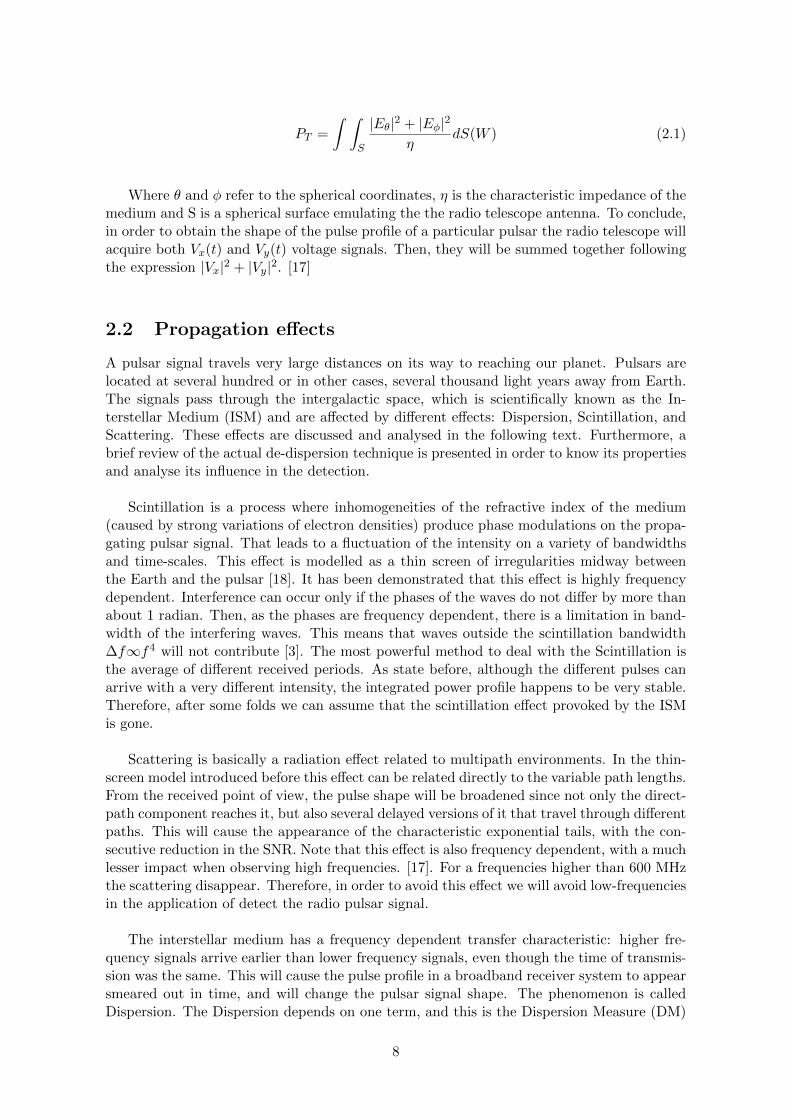
2.2 Propagation effects

A pulsar signal travels very large distances on its way to reaching our planet. Pulsars arelocated at several hundred or in other cases, several thousand light years away from Earth.The signals pass through the intergalactic space, which is scientifically known as the In-terstellar Medium (ISM) and are affected by different effects: Dispersion, Scintillation, andScattering. These effects are discussed and analysed in the following text. Furthermore, abrief review of the actual de-dispersion technique is presented in order to know its propertiesand analyse its influence in the detection.

Scintillation is a process where inhomogeneities of the refractive index of the medium(caused by strong variations of electron densities) produce phase modulations on the propa-gating pulsar signal. That leads to a fluctuation of the intensity on a variety of bandwidthsand time-scales. This effect is modelled as a thin screen of irregularities midway betweenthe Earth and the pulsar [18]. It has been demonstrated that this effect is highly frequencydependent. Interference can occur only if the phases of the waves do not differ by more thanabout 1 radian. Then, as the phases are frequency dependent, there is a limitation in band-width of the interfering waves. This means that waves outside the scintillation bandwidth∆f∞f4 will not contribute [3]. The most powerful method to deal with the Scintillation isthe average of different received periods. As state before, although the different pulses canarrive with a very different intensity, the integrated power profile happens to be very stable.Therefore, after some folds we can assume that the scintillation effect provoked by the ISMis gone.

Scattering is basically a radiation effect related to multipath environments. In the thin-screen model introduced before this effect can be related directly to the variable path lengths.From the received point of view, the pulse shape will be broadened since not only the direct-path component reaches it, but also several delayed versions of it that travel through differentpaths. This will cause the appearance of the characteristic exponential tails, with the con-secutive reduction in the SNR. Note that this effect is also frequency dependent, with a muchlesser impact when observing high frequencies. [17]. For a frequencies higher than 600 MHzthe scattering disappear. Therefore, in order to avoid this effect we will avoid low-frequenciesin the application of detect the radio pulsar signal.

The interstellar medium has a frequency dependent transfer characteristic: higher fre-quency signals arrive earlier than lower frequency signals, even though the time of transmis-sion was the same. This will cause the pulse profile in a broadband receiver system to appearsmeared out in time, and will change the pulsar signal shape. The phenomenon is calledDispersion. The Dispersion depends on one term, and this is the Dispersion Measure (DM)

8

[17]. The dispersion measure is constant only for a certain measurement time and position.In other words, as the interstellar medium is not homogeneous, the dispersion measure willchange depending on where and when the observer has taken the measurements. Therefore,every Pulsar has a different Dispersion Measure.

Dispersion can be removed by the process of de-dispersion. There are two known meth-ods to de-disperse the received signal, the first method de-disperses the signal in the timedomain and is called incoherent de-dispersion, the second method employs frequency do-main operations and is called coherent de-dispersion. The computational requirements ofde-dispersing unit are very high [13]. Actually, all the acquisitions from Radio Pulsar Signalsare de-dispersed in order to be processed with a better SNR. That techniques require morethan the 80% of the computational time needed to receive, process and detect the signal.Later on and unlike a lot of researches think, we will see as the de-dispersion process can beavoided. That is due the fact that dispersion doesn’t change the energy of the Radio PulsarSignal but only the shape. In fact, the effect of the Interstellar Medium (ISM) is describedas a phase only filter, as by the Fourier Transform delay in time domain is equivalent tophase shift in the frequency domain.

2.3 Pulsar-Based Navigation System

Pulsar based navigation is not a novel area of research, and might once offer the possibilityto man of safely travelling distances much beyond Earth. Up until now the focus has been onX-ray based pulsar navigation, whereas recent studies focus on the possibility of using radiopulsars. The radio frequency range had been neglected in the past because the pulses wereassumed to be too weak to detect with antennas of a reasonable size. Nowadays, however,due the really good performance of the Matched Filter as a detector [1] [16] and the fasterevolution of the instrumentations on pulsar receivers, the goal of using the Radio Pulsar forreal time navigation appear as a promising trend. Furthermore, not only can be used tolocalize a spacecraft but to localize targets on Earth. Therefore, pulsar-based navigationsystem can be a substitute of the actual navigation systems as GPS or Galileo.

[7] provides an overview of the work that has been done on pulsar navigation and showsthis new direction in pulsar-based navigation research. Since pulsar signals offer such a highstable periodicity, the idea is to use them as beacons for Time of Arrival (TOA) based navi-gation. There two kinds of navigation algorithms that use the extremely accurate periodicityof Pulsars. The first is the Doppler Shifted Navigation, which uses the Doppler effect in theestimated TOA’s in order to localize the target. The other technique is called Period Decaymethod and uses the period decay of the pulsars. These two techniques are explained indetail in [18].

Although some research has been made about building the actual pulsar navigation sys-tem still no practical implementation has been done. In following chapters we will proposea receptor that includes the optimal detector for the pulsar case and the signal processingtechniques that improve the detection performance.

2.3.1 Navigation system challenge

Although seemingly simple in principle, there are several hurdles that are needed to be over-come in realizing such a navigation system. The main challenges when using radio pulsars

9

for navigation are the following:

1. The extremely weak pulsar signal strength that is being used to navigate. The re-ceived signal is completely submerged in Additive White Gaussian Noise, so the Signal-NoiseRatios are very small on Earth. This is because the pulsar signals are emitted many lightyears away from Earth, leading to addition of noise and distortion due to the propagationchannel as will be discussed later.

2. The requirement of receive, process and detect the radio pulsar signal in a few secondsin order to perform a real time navigation. Up to now the processing time to localize thesignal it is higher than 10 minutes. Furthermore, it is needed really big antennas (+10 mdiameter dish-antennas) to receive the radio Pulsar Signal with enough SNR. Nevertheless,due the improvement of the technology (computers and devices with higher computationalcosts), the antennas (possibility to reach higher Bandwidth) and the left of the receptordevices, someday it will be possible to achieve the goal of a pulsar-based navigation system.

2.4 Pulsars Conclusions

In this chapter I have introduced a brief explanation about what is a pulsar and a classifica-tion of them depending on the signal they emit. We also have seen the main characteristicsof the Radio Pulsar signals. That signals appear to be extremely periodic pulses that arriveto the Earth with a very weak intensity and submerged in Additive Gaussian White Noise.However, due their accurate periodicity they have been chosen as a perfect candidates for areal-time navigation system. Moreover, the Wideband feature of that pulses has been shown.Due that Wideband nature, we are able to receive them in a very big frequency range, fromkHz to THz. That will be an important assumption in order to design the optimum signalprocessing techniques. Also it has been stated that Pulsar signals are highly polarized, hencean acquisition of two orthogonal polarizations is enough to obtain the power pulse profile.

After that, the propagation effects has been explained. The ISM causes several frequencydependent unwanted effects on the wideband pulsar signal, such as dispersion, scatteringand scintillation. However, some practical solutions have been given in order to avoid thoseeffects. For example, choosing a adequate observation frequency. Moreover, it has been in-troduced two de-dispersion methods. Although it looks like they will be an important blockof our receptor, we will see as this statement is not true.

Finally, it has been explained the goal of implementing a radio real-time pulsar-basednavigation system. The two main challenge of this aim has been introduced. That challengeare the low-intensity of the received pulsar signal and the requirement of process and detectthe signals in few seconds. After that, two navigation algorithms has been introduced. Thatmethods are the Doppler Shift and the Period Decay, and they both use the extremely pe-riodicity of the radio pulsar signals as a key to localize a target.

In the next section, a summary of the detection theory written by [1] and [22] will beexplained in order to design a detector to estimate correctly the time of arrival of the pulsar.

10

Chapter 3

Detection Theory applied to RadioPulsar Signals

Detection theory deals with techniques to determine how good data obtained from a certainmodel corresponds to a given data set. An example of that can be the radars, where thepresence of a target has to be detected. Another example could be to detect whether a 0 or 1has been sent in a communication system. In this Thesis we will only deal with the detectionof a pulsar signal over one period in presence of noise. Furthermore, we will assume thatthe pulsar signal is deterministic, so the detection will be easier to perform. Otherwise theprocess will be a detection with random processes.

In this section I will summarize the detection theory applied to radio pulsar signals doneby Richard Heusdens in [1] and [22]. As stated, Radio Pulsar emit a high polarised pulsesextremely periodic. But, as these stars are located millions of km from the Earth they ar-rive with a very low intensity. Moreover, when we receive those signals only noise can beobserved due the fact that they arrive submerged in Additive White Gaussian Noise with avery low Signal to Noise Ratio. In order to achieve our goal of using the Radio Pulsar signalfor navigation applications we should assure that we estimate in a correct way the time ofarrival of the pulses.

First of all, in order to find the optimum detector for our applications a basic detectiontheory for deterministic signals is introduced. The fact that we know exactly how the radiopulsar signal is will be very important to choose a detector. Then, the detection theory forradio pulsars signal application will be explained. As we can guess, besides detect the pulsar,we will need to estimate the amplitude of the pulsar profile in order to implement a templateand the Time Of Arrival to localize our target.

3.1 Basic Detection for deterministic signals

The detection for deterministic signals is the simplest case because the prior we know aboutthe signal play in our favour. The main idea behind the detection process is the statisticalhypothesis testing. Given a data set and different hypothesis our aim will be determinewhich model fits the data best. Due the fact that we want to detect one signal (the oneof the pulsar we want to use for localization), we will only consider in this Thesis two Hy-pothesis. The first hypothesis H0 is the case when only random noise is received. In thesecond Hypothesis H1 the deterministic signal is received in presence of the same randomprocess. We will assume that the random process is an additive gaussian noise with 0 mean

11

and covariance matrix Φz. So, we can model our case as:

H0 : y(n) = z(n) n = 0, 1, 2, ..., N − 1

H1 : y(n) = s(n) + z(n) n = 0, 1, 2, ..., N − 1

Being y(n) the discrete received signal, s(n) the discrete deterministic signal and z(n)the noise process modelled as N ∼ (0,Φz). The focus will be put in the probability densityfunctions of the both hypothesis. That will be useful in order to choose one or the otherhypothesis depending if the received belongs to the pdf of the first or second model. In theHypothesis H0 only noise is received. Then we can state that pdfo is:

pdf0(y) = 1

(2π)N2 |Φz |

12exp(−1

2(y − µ)TΦ−1z (y − µ)) = 1

(2π)N2 |Φz |

12exp(−1

2yTΦ−1

z y)

Being µ the mean of y when we only receive noise. As the H1 will be the hypothesiswhen we receive the deterministic signal submerged in gaussian noise, the probability densityfunction of these model will be also gaussian with a non-zero mean. Therefore,

pdf1(y) = 1

(2π)N2 |Φz |

12exp(−1

2(y−µ)TΦ−1z (y−µ)) = 1

(2π)N2 |Φz |

12exp(−1

2(y−s)TΦ−1z (y−s))

In the next figure 3 we can observe the probability density functions of one both hy-pothesis. They are almost identical due the fact that they have the same random Gaussianprocess. The only difference is that the one of the hypothesis 1 is shifted s (being s the meanof the Hypothesis H1).

F igure 3. Distributions of the Hypothesis H0 and H1. Credit Dr. Richard Heusdens

The detector will consist on choosing one of the distributions depending on the data setwe receive, so a threshold will be needed. Looking at the figure 4 we can see how there aretwo possible mistakes we can make when we assess the detection with the threshold. Thefirst one is called miss (II) and is produced when you choose for the hypothesis H0 and, infact, the deterministic signal is received. The other possible mistake is called false alarm

12

(I) and consist on deciding that you have received the deterministic signal (Hypothesis H1)although it is not true. These errors are unavoidable to some extent but may be traded offagainst each other by adjusting the detection threshold. It is not possible to reduce botherrors at the same time once the probability density functions are set. As a consequence, atypical approach to design an optimal detector is to fix one error probability and minimizethe other. In the next figure we can observe the Hypothesis testing errors and their trafe-off.

F igure 4. Hypothesis testing errors and their trade-off adjusting the detection threshold. Credit Dr. Richard

Heusdens

To assess that probabilities we will assume a simplest model where we only receive onesample with amplitude s and that the noise process z is still a gaussian process and whitewith variance σ2

z1 . So, z1 ∼ N(0, σ2z1). So the probability density functions will be:

pdf0(y1) = 1√2πσ2

z1

exp(− y2

2σ2z1

)

pdf1(y1) = 1√2πσ2

z1

exp(− (y−s)22σ2z1

)

Now it is possible to compute the probability of false alarm as the probability that y1 isbigger than the threshold and in fact we are not receiving the desired signal. That can bestated as:

PFA = P (y1 > γ |H0) =

∫ ∞γ

1√2πσ2

z1

exp(− y2

2σ2z1

)dy

= Q(γ

σz1)

(3.1)

Being Q(y) the Q-function or complementary cumulative distribution function related tothe complementary (Gauss) error function by:

Q(y) = 12erfc(

y√2)

13

As the Q-function decreases when y increases we will decrease the probability of falsealarm when the threshold is increased or when the noise variance decreases. By the sameprocess we can calculate the probability of detect correctly the signal without any mistake.That can be computed as the probability that the y1 is bigger than the threshold if we receivethe deterministic signal.

PD = P (y1 > γ |H1) =

∫ ∞γ

1√2πσ2

z1

exp(−(y − s)2

2σ2z1

)dy

= Q(γ − sσz1

)

(3.2)

As we were expecting, due the probability density functions are identical but with dif-ferent mean, the probability of detection has the same function as the probability of falsealarm but with a shift in the Q-function. So, setting a probability of false-alarm our aimwill be to choose the optimum algorithm to optimize the detection performance.

There are several kind of different detectors algorithm to choose depending on our goal,but we are going to consider the classics ones. One of the more important detector is theBayesian. It work taking into account the probability of having the different hypothesis,so a prior information about the statistics of the models are needed. In other words, is anstatistical approach that quantify trade-offs between various hypothesis using probabilitiesand costs that accompany such decisions. We will not use that kind of detector due the factthat for our applications we do not have any statistical prior information. The next kindof detector is the Neyman-Pearson detector. That detector does not require any statisticalprior information and performs the optimal probability of detection for a fixed false-alarmprobability. However, the Neyman-Pearson criterion will only be true if we fully know thedeterministic signal s. Hence, if there are not variables to estimate in the desired signal. Forour applications we need to estimate the amplitude and time of arrival of the received data-set, so the Neyman-Pearson will be unrealisable. Finally, the Generalised Likelihood RatioTest will be explained. That technique is used to detect the desired signal even when someof the parameters of that signals are not known. In fact, the GLRT is equal as the NeymanPearson detector but replacing the unknown parameters by their maximum likelihood esti-mates (MLE’s). Unlike the Neyman Pearson detector there is no optimality associated withthe GLRT in practice. Nevertheless, it can be shown that asymptotically, the GLRT is a uni-formly most powerful (UMP) test, meaning that asymptotically (N →∞) it gives the highestprobability of detection given a false alarm probability PFA (being N the length of the data).

3.2 Generalised Likelihood Ratio Test applied to Radio Pul-sar Signals

In order to choose a detector we have to take into account that some of the parametersof the Radio Pulsar Signals are unknown. The proposed technique will be the GeneralisedLikelihood Ratio Test. It consist on estimating the unknown parameters using the maximumlikelihood estimates (MLE’s) and incorporate them in the pdf of the different Hypothesis.Then, the likelihood ratio test will be created with those pdf in order to compute the Test

14

Statistics. On the contrary as the Bayesian approach, the GLRT does not require any priorinformation about the unknown parameters. In practice, the GLRT appears to be morewidely used due to its ease of implementation and less restrictive assumptions. Furthermore,the Bayesian approach requires multidimensional integration, which is usually not possiblein closed form.

The GLRT criterion says that we should construct our decision rule to have maximumprobability of detection while not allowing the probability of false alarm to exceed a certainvalue. So, it states that when performing a hypothesis test between two hypotheses H0(y)and H1(y), then the H0 is rejected in favour of H1 when

LGLRT = pdf1(y;θ1)

pdf0(y;θ0)> ξ

Where ξ is such that

PFA(y) =∫

(y|LGLRT (y)>ξ) pdf0(y)dy = α

Being LGLRT (y) the likelihood ratio, pdf the probability density functions of the Hy-pothesis, θ1 and θ0 the MLE estimation of the unknown parameters and ξ the threshold. Inthis section is going to apply that detector to the Radio Pulsar Signal case. Radio PulsarSignals are deterministic signals with unknown amplitude and TOA submerged in AdditiveWhite Gaussian Noise.

The estimation of the amplitude will not be a problem since we will use MLE to estimateit. Later on we will see how that amplitude is obtained. Nevertheless, the TOA will be adifferent matter, and for that reason it will be necessary to use the GLRT instead of theNeyman-Pearson detector. The two different Hypothesis we have in our scenario are

H0 : y(n) = z(n) n = 0, 1, 2, ..., N − 1

H1 : y(n) = Dτos(n) + z(n) n = 0, 1, 2, ..., N − 1

Where D denote the (circular) unit shift operator. That is, (Ds)(n) = s(n−1modN), andthus Dks(n) = s(n−kmodN). Since ‖Dks‖2 = ‖s‖2 , we conclude that D is a unitary opera-tor and therefore (Dk)T = D−k. As we have stated, the suboptimal test will be the General

Likelihood Ratio Test, where we will decide for the Hypothesis H1 if LGLRT = pdf1(y;τo)pdf0(y) > ξ.

We will perform the detection over one period of the radio pulsar signal because due thegood performance of the Epoch Folding. In the remainder of this report, we will refer toone period of the pulsar signal as the pulsar profile. As the noise is white, if we develop theLikelihood Ratio Test we will obtain:

T (y) = yTDτos > σ2z ln(ξ) + 1

2εs = γw

15

Being T(y) the Test Statistics function. That can be seen as the correlation of the re-ceived signal with a template of the deterministic pulsar signal after estimating the amplitudeand the TOA. In fact, the test statistics can be seen as a filter with a shifted template as ah(n). So, we can state that the implementation of that Test Statistics is the Matched Filter.This is something normal since we know that the Matched Filter is the optimum filter for asignal submerged in AWGN.

As stated before, the amplitude of the template will be easy to compute. We only have

to perform the MLE of the amplitude as a = yT ssT s

and multiply that resultant value to thetemplate. So, we will decide for H1 if the value of that test statistics is higher than thethreshold γw.

But there are a problem, and it is that the MLE estimation of the TOA is argmaxτ yTDτs,

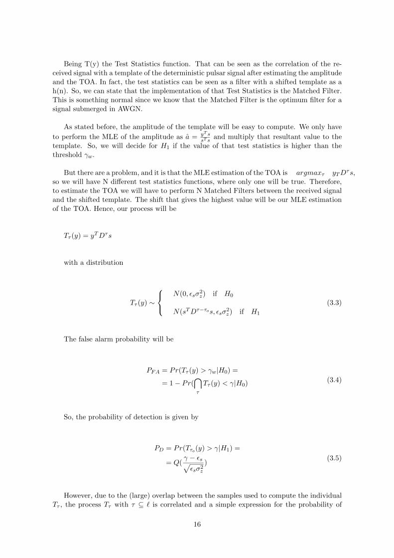
so we will have N different test statistics functions, where only one will be true. Therefore,to estimate the TOA we will have to perform N Matched Filters between the received signaland the shifted template. The shift that gives the highest value will be our MLE estimationof the TOA. Hence, our process will be

Tτ (y) = yTDτs

with a distribution

Tτ (y) ∼

N(0, εsσ

2z) if H0

N(sTDτ−τos, εsσ2z) if H1

(3.3)

The false alarm probability will be

PFA = Pr(Tτ (y) > γw|H0) =

= 1− Pr(⋂τ

Tτ (y) < γ|H0) (3.4)

So, the probability of detection is given by

PD = Pr(Tτo(y) > γ|H1) =

= Q(γ − εs√εsσ2

z

)(3.5)

However, due to the (large) overlap between the samples used to compute the individualTτ , the process Tτ with τ ⊆ ` is correlated and a simple expression for the probability of

16

false-alarm does not exist. Indeed, we have

Pr(⋂τ Tτ (y) < γ|H0) =

∫ γ∞ ...

∫ γ∞

1

(2π)N2 |ΦT |

12exp(−1

2yTΦ−1

T y)dy

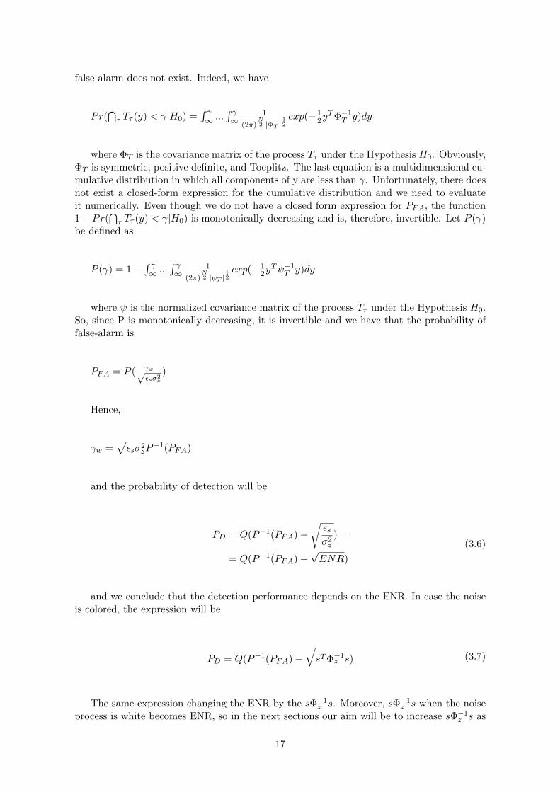
where ΦT is the covariance matrix of the process Tτ under the Hypothesis H0. Obviously,ΦT is symmetric, positive definite, and Toeplitz. The last equation is a multidimensional cu-mulative distribution in which all components of y are less than γ. Unfortunately, there doesnot exist a closed-form expression for the cumulative distribution and we need to evaluateit numerically. Even though we do not have a closed form expression for PFA, the function1− Pr(

⋂τ Tτ (y) < γ|H0) is monotonically decreasing and is, therefore, invertible. Let P (γ)

be defined as

P (γ) = 1−∫ γ∞ ...

∫ γ∞

1

(2π)N2 |ψT |

12exp(−1

2yTψ−1

T y)dy

where ψ is the normalized covariance matrix of the process Tτ under the Hypothesis H0.So, since P is monotonically decreasing, it is invertible and we have that the probability offalse-alarm is

PFA = P ( γw√εsσ2

z

)

Hence,

γw =√εsσ2

zP−1(PFA)

and the probability of detection will be

PD = Q(P−1(PFA)−√εsσ2z

) =

= Q(P−1(PFA)−√ENR)

(3.6)

and we conclude that the detection performance depends on the ENR. In case the noiseis colored, the expression will be

PD = Q(P−1(PFA)−√sTΦ−1

z s) (3.7)

The same expression changing the ENR by the sΦ−1z s. Moreover, sΦ−1

z s when the noiseprocess is white becomes ENR, so in the next sections our aim will be to increase sΦ−1

z s as

17

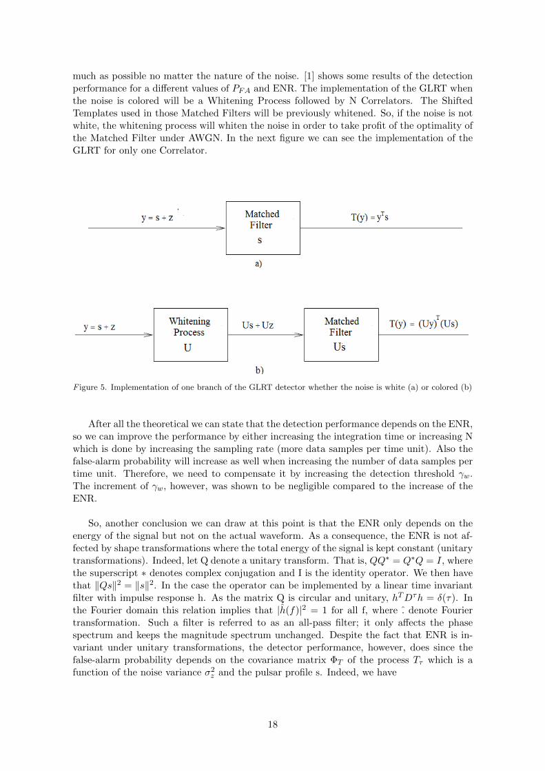
much as possible no matter the nature of the noise. [1] shows some results of the detectionperformance for a different values of PFA and ENR. The implementation of the GLRT whenthe noise is colored will be a Whitening Process followed by N Correlators. The ShiftedTemplates used in those Matched Filters will be previously whitened. So, if the noise is notwhite, the whitening process will whiten the noise in order to take profit of the optimality ofthe Matched Filter under AWGN. In the next figure we can see the implementation of theGLRT for only one Correlator.

F igure 5. Implementation of one branch of the GLRT detector whether the noise is white (a) or colored (b)

After all the theoretical we can state that the detection performance depends on the ENR,so we can improve the performance by either increasing the integration time or increasing Nwhich is done by increasing the sampling rate (more data samples per time unit). Also thefalse-alarm probability will increase as well when increasing the number of data samples pertime unit. Therefore, we need to compensate it by increasing the detection threshold γw.The increment of γw, however, was shown to be negligible compared to the increase of theENR.

So, another conclusion we can draw at this point is that the ENR only depends on theenergy of the signal but not on the actual waveform. As a consequence, the ENR is not af-fected by shape transformations where the total energy of the signal is kept constant (unitarytransformations). Indeed, let Q denote a unitary transform. That is, QQ∗ = Q∗Q = I, wherethe superscript ∗ denotes complex conjugation and I is the identity operator. We then havethat ‖Qs‖2 = ‖s‖2. In the case the operator can be implemented by a linear time invariantfilter with impulse response h. As the matrix Q is circular and unitary, hTDτh = δ(τ). Inthe Fourier domain this relation implies that |h(f)|2 = 1 for all f, where . denote Fouriertransformation. Such a filter is referred to as an all-pass filter; it only affects the phasespectrum and keeps the magnitude spectrum unchanged. Despite the fact that ENR is in-variant under unitary transformations, the detector performance, however, does since thefalse-alarm probability depends on the covariance matrix ΦT of the process Tτ which is afunction of the noise variance σ2

z and the pulsar profile s. Indeed, we have

18

PD =∫∞γw

1√2πεsσ2

z

exp(− (y−εs)22εsσ2

z)dy

Although the distribution in the last expression does not depend on the shape of s, thedetection threshold γw given by γw =

√εsσ2

zP−1(PFA) does since it is a function of the

complementary cumulative distribution P which depends on ΦT . We conclude that thethreshold γw is maximal whenever the process Tτ is uncorrelated. This leads us to the ap-parent contradictory conclusion that we obtain the best detection performance for highlycorrelated data and worse performance for uncorrelated data. In terms of the correlationfunction of the pulsar profile this means that the performance goes down the more ”peaked”the correlation function is. The detection performance is, however, invariant under all-passfiltering. Indeed, let Sz denote the power spectral density of the noise process z and let Ydenote the process after all-pass filtering. We then have that SY (f) = |h(f)|2Sz(f) = Sz(f)for all f and therefore ΦY = Φz. Similarly, the correlation function Rss is not affected byall-pass filtering and we conclude that ΦT is invariant under all-pass filtering. As a conse-quence, P, and therefore γw, is invariant under all-pass filtering. An example of the use ofall-pass filtering is the dispersion in pulsar signals. Based on our discuss above we concludethat, in contrast to what people currently do, there is no need to de-disperse the observeddata, thereby saving approximately 80% of the total computational load currently neededfor detecting radio pulsars. [1]

The last conclusion we draw here is that, as mentioned before, the probability of detect-ing the signal is not equivalent to the probability of estimating the unknown TOA correctly.Indeed, we only correctly estimate τ when the maximum occurs at the correct value τ = τo.To see what is the effect of the shape of s on the estimation of τo, we consider the proba-bility that the maximum of Tτ occurs at the correct value τ = τo under the Hypothesis H1

and exceeds the detection threshold γw. Obviously, this probability, which we will denoteby Pτo , is given by the probability that Tτo(y) > γw and Tτ (y) < Tτo(y) for all τ 6= τo. Hence,

Pτo = Pr(Tτo(y) > γw &&⋂τ 6=τo

Tτ (y) < Tτo(y)|H1) =

=

∫ ∞γw

(

∫ yτo

−∞...

∫ yτo

−∞

1

sqrt(2π)N2 |ΦT |

12

exp(−1

2(y − µT )TΦ−1

T (y − µT ))dyτo

(3.8)

where µT = sTDτ−τos and dyτo = dyo...dyτo−1dyτo+1...dyTo−1. By inspection of the lastequation we conclude that Pτo depends on ΦT , µT , and γw only, which all are invariantunder all-pass filtering. As a consequence, de-dispersing the received pulsar signal does nei-ther affect the probability of detection nor the probability of correctly estimating the timeof arrival τo. [1]

In contrast to what we concluded for the probability of detection PD, the probability Pτoof correctly estimating the unknown TOA is maximal in the case the process Tτ , τ ∈ `)is independent (peaked correlation function) and minimal in case the process is fully corre-lated. The fact that the probability of correctly estimating the unknown TOA is maximalfor statistically independent random variables does not imply that this results in the bestestimation of τo. In order to compare the effect of shape transformations of the estimation itis shown in [1] the plots of the mean and variance of the MLE estimator of the time of arrival

19

for the different shape transformations. The best results are obtained for the smoothed pul-sar profile. All-pass filtering, however, has no effect on the performance, as expected. As therandomized signal is the one with a more independent variables (a really high and narrowpeak in the correlation function), Dr. Heusdens has proved how the fact that the TOA ismaximal for statistically independent random variables does not imply that this results inthe best estimation. Moreover, as expected, the TOA estimation performance increases withthe ENR.

Figure 6. MLE of the TOA τo. Credit Richard Heusdens

3.3 Conclusions of the Detection Theory

From that section we have obtained a lot of important conclusions in order to make feasibleour aim of real time navigation using Radio Pulsar Signals. First, we have stated that thebest approach for our case will be the performance of Neyman-Pearson detector. That isbecause the Neyman-Pearson gives the best detection performance once the probability offalse alarm is fixed. However, as we need to estimate the Time Of Arrival of the signal, it isnot possible to use that detector. So, it has been found a suboptimal detector, the GLRT.Assuming that the received signal is the radio pulsar pulse submerged in white noise, theGLRT will correlate N times (being N the length of on period) that received signal with theshifted replica or template of the radio pulsar Dτs. After doing that, we will estimate our

20

TOA as the shifted value τ that has given the highest correlation. Besides, we will decidethat the signal has been detected if that correlation value is above a threshold γ. If thenoise is colored, we have seen as the Detection Performance will depend on sΦ−1

z s. So, theimplementation of the GLRT when the noise is colored will be a Whitening Process followedby N Correlators.

Furthermore, it has been found the expressions for the detection performance and theestimation of the time of arrival, stating that we have to increase the ENR (if the noiseprocess is white) or the GENR (if the noise process is colored) as much as possible. In theprevious Thesis and Reports the aim has been to find the techniques that improve the SNRof the signal. Nevertheless, the SNR will not have any effect in the detection performance.Also it has been shown that for a ENR-GENR of 16 dB, the detection of the pulsar and theestimation of the time of arrival will be almost perfect. So, in the next chapters our aimwill be to find which signal processing techniques improves the GENR of the process assum-ing that the Radio pulsar signals have a Wideband nature. The detection theory explainedadded to the signal processing techniques will lead to a theoretical optimum receptor for thedetection of radio pulsar signals. That detector is proposed in the chapter 8.

The last conclusion and more important of that section is the fact that the GLRT de-tector and MLE estimation of the TOA processes does not depend on any all-pass filteringoperation. As the de-dispersion process can be modelled as a all-pass filtering, that meansthat performing the de-dispersion method will not have any effect in the detection perfor-mance neither the estimation of the TOA. That is a really important result since up to 80%of the computational cost dedicated to process the radio pulsar signal is spent in that process.

21

Chapter 4

Radio Pulsar Signal Model

Figure 7. Block Diagram of the receiver and the Analogue to Digital Converter

This section focus in the original properties of the Radio Pulsar signal and the Noiseprocess. From now on I will assume that the received Radio Pulsar Signal is a deterministicwideband signal with unknown amplitude and Time Of Arrival submerged in Additive WhiteGaussian Noise. Therefore, we can model it as:

yr(t) = asr(t− τ) + zr(t)

Being s(t) the Radio Pulsar signal, z the noise process, a the unknown amplitude and τthe unknown Time Of arrival. In the Detection Theory section we have seen how to estimatethe Amplitude and the time of arrival of the signal. In the next subsections we are goingto assume that the amplitude and the time of arrival are known in order to compute in aneasy way the ENR and GENR of the signal. Hence, the signal before passing through theanalogue Low-Pass Filter will be:

yr(t) = sr(t) + zr(t)

22

4.1 Filtered Analogue Signal

F igure 8. Power Spectrum of the AWGN and its Autocorrelation function

From now on, this Thesis will refer to the analogue filtered signal as

ya(t) = sa(t) + za(t)

Being ya the signal received and filtered with an analogue Low-Pass Filter, sa the deter-ministic wideband signal and za the Additive White Gaussian Noise. As we assume that theRadio Pulsar signals are completely known, we model them as deterministic with an energy

εa =∫∞−∞ |sa(t)|

2dt = 12πfs

∫∞−∞ |Sa(w)|2dw

The second term of the equation is only true if we are working with angular frequencyin rad/s. On the other hand, the noise is a stochastic White Gaussian signal N ∼ (0, σ2

za)with 0 mean and variance σ2

za . As state before, ya is composed by the pulsar and noisesignal, Band-limited to the Bandwidth of the analogue low-pass filter. In this first part ofthe Thesis we will assume that the antenna is ideal with a Bandwidth equal as the cut-offfrequency of the Analogue Low-Pass Filter. Later on, we will observe how under that as-sumption the analogue Low-Pass Filter is useless from a detection performance point of view.

As the noise is the principal problem why we can’t correctly detect the signal, we aregoing to focus on its properties. As stated, the received noise is a continuous time AdditiveWhite Gaussian process with 0 mean, variance σ2

za and spectral density No. Therefore, thepower spectrum of the noise is:

Sza(w) =

{No for |w| ≤ 2πB0 otherwise

(4.1)

where w is the angular frequency in rad/s. If we compute the inverse of the FourierTransform of the Power Spectrum we will obtain the autocorrelation function of the noise:

23

Rza(t) =1

2π

∫ ∞−∞

Sza(w)ejwtdw =1

2π

∫ 2πB

−2πBNoe

jwtdw

=No

πtsin(2πBt) = 2BNosinc(2πBt)

(4.2)

Therefore, the variance of the noise process is σ2za = Rza(0) = 2BNo, with B the Band-

width of the signal and No the Power Spectral density of the noise. Looking at the PowerSpectrum and the Autocorrelation function of the noise processes after passing the signalthrough some processing techniques we will be able to know the variance of the noise andcalculate the variations of the ENR.

4.2 A/D converter

Just before starting to process the signal, it is passed through an the A/D Converter withsampling frequency fs in order to work in the digital domain. The reason of sampling thesignal is to have more facilities to process it with a lower cost and a flexible digital hardware.At the end of the A/D converter we will have:

y(n) = ya(nTs) = sa(nTs) + za(nTs) = s(n) + z(n)

where Ts is the inverse of the sampling frequency fs called sampling period. Hence, thediscrete signals s and z are obtained by sampling sa and za with the sampling Nyquist ratefs = 2B. We use this sampling frequency in order to avoid aliasing and keep the whiteproperty of the noise process. Later on we will see how important is to have AWGN from aprocessing time point of view.

As we have seen in the last section is used the un-normalised frequency w as the variablefor the representations of the signals in the frequency domain, being w = 2πf . To changebetween time and frequency domain it is used the Discrete time Fourier Transform:

y(n) = 12πfs

∫ 2πfs0 Y (w)ejwnTsdw

Y (w) =∑∞

n=−∞ y(n)e−jwnTs

First of all, to assess the ENR of the process y we will focus on the deterministic signal s.As it is known, when a signal goes into an A/D converter, it loses information, and its visiblespectra will be limited to the sampling frequency, 2πfs. Besides, in the frequency domainappears images of the signal every 2πkfs (with k a integer number, creating aliasing if theNyquist Sampling Frequency, or a bigger rate is not used). As we stated before, the Nyquistsampling frequency is used in this section, so no aliasing will be obtained. Following that,the spectra of the discrete signal compared to the spectra of the previous analogue signal is:

24

S(w) =∑∞

n=−∞ s(n)e−jwnTs = fs∑∞

n=−∞ Sa(w + 2πkfs)

So we can find an expression of the energy of the deterministic sampled signal s in com-parison with the energy of the analogue filtered signal sa as:

εs =∑n

|s(n)|2

∗=

1

2πfs

∫ 2πfs

0|S(w)|2dw

=fs2π

∫ 2πfs

0|∞∑

k=−∞Sa(w + 2πkfs)|2dw

∗∗=fs2π

∫ πfs

−πfs|Sa(w)|2dw

=fs2π

∫ ∞−∞|Sa(w)|2dw

= fsεsa

(4.3)

* By Parseval Theorem that states that the energy of the signal in time is preserved in the frequency domain

as well.

** Taking into account that Sa(w) do not have any contribution in w /∈ [−πfs, πfs]. No aliasing.

In this formula has been assumed that the bandwidth of the signal sa does not exceedhalf of the total visible spectra 2πfs. As we can observe, the energy of the sampled signalincreases with the sampling frequency in comparison to the analogue one. This result showsthat increasing the fs the energy of the process is improved, even when the bandwidth ofthe signal is not increased.

On the other hand, to check the behaviour of the discrete time noise z, we are going tolook to its Autocorrelation function:

Rz(k) = z(n) ∗ z(n+ k) = z(nTs) ∗ z((n+ k)Ts)

= Rza(kTs) = 2BNosinc(2πBkTs)

= 2BNosinc(2Bπk

2B)

= 2BNosinc(kπ) = 2BNoδ(k)

(4.4)

Being δ(k) the Kronecker delta. That happens because sampling the noise with theNyquist sampling frequency preserve the Whiteness of the Noise. We can also observethat the variance of the discrete Noise will remain the same as before passing the sig-nal through the A/D converter no matter the sampling frequency used. Therefore, σ2

z =Rz(0) = fsNoδ(0) = 2BN0 = σ2

za . Finally, computing the Power spectrum of the Noise asthe discrete-time Fourier Transform of the Autocorrelation Function, we have:

25

Sz(w) =

{fsNo for |w| ≤ πfs0 otherwise

(4.5)

As we can observe, the shape of the Power spectrum of the noise remains equal, althoughthe value of the discrete power spectral density is increased by the factor fs. Once obtainedthe values of the energy of the sampled signal s and the variance of the noise z, ENR iscomputed:

ENR =εsσ2z

=fsεsaσ2za

=fsεsa2BNo

=fsεsafsNo

=εsaNo

(4.6)

In the next subsection the term GENR is introduced. It is a Ratio to assess the ENRwhen the noise is not white. As we have seen in the Detection Theory, this Ratio assessthe detection performance of the GLRT Detector. As we will see later, one way to improvethe GENR is increasing the observation time of the signal to be detected, so εsa will beincreased. The problem is that we will focus on detecting the Pulsar signal over one period,so we will not be able to increase the energy of the signal integrating over a longer time span.

4.3 Generalised Energy To Noise Ratio

To assess the behaviour and the improvement of the signals after performing some signalprocessing techniques, the scientific use different ratios. The most used is the SNR or Signalto Noise ratio, being the relation between the power of the desired signal and the varianceof Noise.

SNR =Psσ2z

(4.7)

Although up until now the researchers have been using this radio to assess the Radio pul-sar signals behaviour, in this report we are going to use other two ratios, the Energy to Noiseratio and the Generalised Energy to Noise ratio. As it has been explained in the DetectionTheory chapter, the detection performance only depend on the Generalised Energy to Noiseratio, and, in some cases, on the Energy to Noise Ratio. The term Generalised Energy toNoise Ratio has not been used before, but it describe the relation between the signal and thecovariance matrix of the noise. Then, we are going to refer to Generalised Energy to Noiseratio of the signal y = s+ z as:

GENR = sTΦ−1z s (4.8)

26

with

Φz = E((z − z)(z − z)T )

the covariance of the noise process and s the desired signal. We can see that if thenoise is AWGN with 0 mean and covariance matrix Φz = σ2

zI, so Φ−1z = 1

σ2zI, the GENR

becomes the relation between the energy of the signal and the variance of the noise. Therefore

GENR = sTΦ−1z s =

sT s

σ2z

=εsσ2z

= ENR (4.9)

The GENR takes into account the color of the noise to assess the detection performance.From now on, Generalised Energy to Noise Ratio will be used to measure up whether thedifferent signal processing algorithms increase or not the detection performance.

27

Chapter 5

Theoretical Signal ProcessingTechniques

Figure 9. Block Diagram of the Signal processing techniques applied to the discrete-time signal

The signal from the Radio pulsar is received submerged in AWGN and it is not possi-ble to see or detect it without some processing. In this chapter we introduce some basicsignal processing techniques to check if the ENR and GENR of the pulsar signal increase.The algorithms explained will be Epoch Folding, an average of the received signal at theexact period of the pulsar; Low-Pass Filtering, to eliminate the high frequencies of the sig-nal; Downsampling, to change the sampling rate of the signals and therefore, the length ofthe data; decrease and increase the Bandwidth of the Antenna (and therefore, the cut-offfrequency of the Analogue filter); and Oversampling/Undersampling, passing the analoguesignal to the A/D converter with a sampling frequency higher/smaller than the Nyquist onefs.

Downsampling can also be seen as a process that changes the bandwidth of the antennaand the sampling frequency of the A/D converter, an interesting feature that will help usto increase the ENR of the rotating star pulse without increasing the observing time. Thatresult could be good to perform a real-time detection of the pulsar for navigation applications.

5.1 Epoch Folding

Epoch Folding is a Signal Processing technique used to decrease the variance of the uncor-related noise while keeping the energy/power of the desired signal. Epoch folding consist onchoosing a range of periods, and average the data at those periods. The algorithm assumesthat we know the periodicity, T , of the signal. The first step consist on breaking the receivedsignal in intervals of time T . Then, sum all these clipped signals together and divide theresultant signal by the number of foldings, K. No matter if the signal is narrowband or

28

wideband, because we are not clipping any frequency spectrum of the signal provided theright period to perform the folding is used. So, the shape, amplitude, energy and power ofthe signal will remain the same no matter how many folds you do.

In the case of Radio Pulsar signals, although they arrive with a very precise periodicityto the Earth, their amplitude can vary significantly over time due to the scintillation effectsprovoked by the ISM. Nevertheless, the averaged pulsar profile remains very stable, allowingus to perform the Epoch Folding without loosing any information of the signal not in timeneither in frequency domain. As it has been explained, the noise will be additive, white andgaussian with 0 mean, variance σ2

z and uncorrelated. Is the last feature the important forthe success of this technique, because averaging AWGN uncorrelated noise leads to a lineardecrease of the noise variance with the number of folds. Furthermore, the noise is still whiteafter passing through the averaging, so the GENR of the received data will increase. In theFigure 10 we can observe the process of epoch folding.

Figure 10. Epoch Folding algorithm performed to a periodic signal submerged in uncorrelated noise.

As we are going to perform this algorithm to a discrete signal, let me consider r as thediscrete signal with KTfs samples, being K the number of folds and Tfs the number ofsamples in one period. The next step is breaking the data in a sequence of discrete signalsyk of length L, being L = fsT . As we have stated, yk = sk + zk with zk ∼ N(0, σ2

z) anAdditive White Gaussian Noise and sk the desired signal with length L. So, performing theEpoch Folding we have:

x(n) =1

K

K−1∑k=0

yk(n)

=1

K

K−1∑k=0

sk(n) +1

K

K−1∑k=0

zk(n)

≈ s(n) + z(n)

(5.1)

29

Being s the desired signal and z the average of K noise signals of length L. Lookingat the desired signal we can see as s(n) = sk(n), so as we said, the average signal profiledoesn’t change. Note that z(n) decreases while K increases. Hence, if we keep increasing thenumber of foldings, the noise background will keep decreasing. Therefore, the signal will bemore visible and the SNR, ENR and GENR will increase. In the limit case when K = ∞,the noise z(n) = 0, so the processed signal will be the pulsar signal.

Let’s focus on the ENR and GENR of the folded signal x = s + z knowing that theenergy of the sampled pulsar signal is εs, the variance of the noise before doing the folding

is σ2z = fsNo and the variance of the folded noise is σ2

z = σ2zK .

ENR =εsσ2z

=εsσ2zK

=fsεsaσ2zaK

=fsεsa2BNoK

=fsεsafsNoK

=KεsaNo

(5.2)

GENR = sTΦ−1z s =

sT s

σ2z

=εsσ2zK

=KfsεsafsNo

=KεsaNo

= ENR (5.3)

We can observe how the ENR and GENR of the folded signal has increased in a factor ofK if we compare them with the ENR and GENR of the unprocessed signal. The reason whythe Epoch folding improve the GENR and therefore, the detection performance is becausethis algorithm doesn’t modify the Power spectrum shape of the Noise, so it keep being white.In the next sections we will see the results of the performance of Epoch Folding with up to195 folds to the real pulsar signal B0329+54 and how that increase the ENR in a linear way.

However, the main goal of detecting the pulsar is to use it for Real-Time NavigationSystems. So although we can obtain a big value of ENR increasing K, it will also increasethe observing time, making impossible the real time navigation. In order to minimize thatproblem, nowadays the scientific are studying and using the millisecond pulsar. As I statedbefore, they arrive with less intensity than the other ones, but with a periodicity aroundone ms, so you can perform one thousand foldings loosing only 1 second in the process. Inthe next subsection we are explaining another signal processing techniques in order to knowhow to keep improving the GENR of the signal without increasing the computational costtoo much. Because although Epoch Folding can increase in a factor of 1000 the ENR of themillisecond pulsar with only one second of observation time, is not enough to perform a gooddetection of the time of arrival of the pulsar.

5.1.1 Integration in Time

The researchers usually use another kind of process at the same time they perform the EpochFolding. That process can be seen as an integration of the signal in time. That techniqueis used to improve the SNR by a factor of thousands, so it is very useful to see the pulsarprofile of the signal without noise. Furthermore, it is possible to reduce the length of thesignal from millions of samples to only a thousand. As stated, that technique is usually usedat the same time as the Epoch Folding although is not the same signal processing technique.

30

However, it also has some drawbacks. As we will see, the Integration process is formedby two blocks of Average process + decimation, so the high frequencies of the signal willdisappear. It is known that the Radio Pulsar signal has a wideband nature, so with thatintegration we will eliminate information of our received pulsar. Moreover, it will be seenas this technique does not improve the detection performance since the ENR and GENR ofthe signal will not be improved. Nevertheless, later on it is going to explain why it can beuseful for our application of real time navigation.

That integrating process consist on separating a signal of N samples in blocks of Nchan2 ,

being Nchan twice the number of frequency channels that the resultant signals will have.Then, those Nchan

2 samples will be associate to a one of the nbins different bins. The number

of bins will be the length of our resultant signal after doing this process. Once the Nchan2

samples has been bound to a bin, the energy of that signal is computed for every frequencychannel and stored in those bins. That process will be repeated until the last samples ofthe period has been processed. As we can see, you can repeat that process K times in orderto merge the Epoch Folding Technique with the Integration in Time. That technique leadto a really good results in SNR as it can be observed in the pulsar profiles from the EPNDatabase [5]. So, at the end a signal with nbins and Nchan

2 different channels will be ob-tained. Now, if you merge all the frequency channels to have only one averaged channel, theresultant signal can be used to perform some signal processing experiments. Some peoplethink that due the fact the SNR has been improved by a order of thousands that meanthat the signal will be easier to detect, but that is not true. As it has been stated in the de-tection theory chapter, the detection performance will depend on the ENR and not the SNR.

So, if we analyse that Integrating process carefully, it is trivial that for Wideband Signalswe can model it with 2 processing techniques. The first block is an average process (witha performance equal as an Epoch Folding) with a factor N

2nbins.The second is Decimation

process with a decimation factor of Nnbins

. As we will see later, and assuming that the signalis wideband, those two processes will decrease the GENR/ENR by a order of 2. Therefore,that process is not useful from a detection performance point of view.

Figure 11. Block representation of the Integration in Time Process. It is shown the length of the signal after

passing through each block.

The conclusion of this section is that with the Integration in Time technique we aredecreasing the detection performance. That can be seen as something bad. Nevertheless, inour application to perform the detection of radio pulsar signals in real time may be useful.First of all, the Radio Pulsar signal has a Wideband nature, so it is possible to receive thepulsar profile from almost all the spectra and with different Bandwidths. That means thatif we eliminate the high frequencies of the radio pulsar signal we will still see the pulsar al-

31

though with a less amplitude. So, whenever the Template has the same shape and frequencyinformation that our received signal, the loss of high frequencies will not be a problem. Fi-nally and most important, since the goal will be to achieve the enough ENR/GENR to beingable to correctly detect the signal with the less computation cost possible, the reduction ofsamples may be useful due the fact that we will work with a signal of a thousand samplesinstead of millions, so the processing time of the next signal processing steps will be reducedin a factor of hundred of thousands. Moreover, only losing 3 dB of ENR. So, depending onthe computational cost required to perform that integration it will be useful to perform it. Inthe last chapter an optimal receptor will be proposed. Although that technique will not bein the first version of the proposed receptor, it will be a part of the second proposed receptor.

5.2 Low-Pass Filtering

Figure 12. Spectra of the Low-Pass Filter H(w) with cut-off frequency f .

The main purpose of this Thesis is to find the signal processing techniques that improvesthe performance of the GLRT. In this section I focus on the Low-Pass Filtering as the firststep of downsampling. So, therefore, the cut-off frequency of the filter will be fc = 2πB/M .That filter will filter out all the high frequencies of the noise, reducing the variance of it.Also, as the pulsar signal is Wideband, the filter will affect the Pulsar signal, eliminatingsome spectral content and reducing its energy.

We will assume that the frequency response H(w) of the low-pass filter is given by:

H(w) =

{1 for |w| ≤ πfs

Mα otherwise

(5.4)

32

With α→ 0. We are not assuming an ideal Low-pass filter because to assess the GENRwe need to compute the inverse covariance matrix of the filtered noise. The fact is that whenyou low pass filter the noise, it becomes colored. That means that the covariance matrix willnot be the variance of noise multiplied by the identity matrix. Nevertheless, we know thatthat covariance matrix will be Toeplitz and Hermitian. Moreover, it allows a singular valuedecomposition, so we will assume it has eigenvalues λi. To make that matrix invertible, weneed to assure that ∨λi > 0. One of the solutions to assure that, is putting a non-zero valueto all the frequencies of the filter. That is why we can see the factor α in the equation 5.4.But in the cases where the filter have a very small cut-off frequency (M big), this solution isnot enough. So, taking into account the results from [2], we also assume that the length of thefilter is small enough to allow us to compute the inverse of the covariance matrix of the noise.

Applying the decimation filter to the discrete signal y = s+ z we will obtain yf = p+ v,where p is the filtered pulsar signal and v is the filtered noise process, both band-limited toa bandwidth 2πB/M with the same sample rate fs as before the filtering. So, the powerspectrum of the filtered noise will be:

Sv(w) =

{fsNo for |w| ≤ πfs

M

α2 for πfsM < |w| < πfs

(5.5)

We can observe that if M > 1 the noise power spectrum will lose the white feature.Therefore, it will be colored and its covariance matrix will not be diagonal. Nevertheless,the Power spectral density has the same value as before the filtering. Knowing Sv(w), we willcompute the Autocorrelation function Rv(k) as the inverse discrete time Fourier transformof it:

Rv(k) =1

2πfs

∫ ∞−∞

Sv(w)ejwkTsdw∗≈ 1

2πfs

∫ πfsM

−πfsM

NofsejwkTsdw

=No

πkTssin(

πk

M) =

NofsM

sinc(πk

M)

(5.6)

* Assuming that the contribution of α2 to the other frequencies are negligible and will not alter the result of

the autocorrelation function of the filtered noise.

Taking into account that Ts = 1fs

. We can see as the variance of the noise process has

decreased by a factor of M: σ2v = Rv(0) = Nofs

M = σ2zM . That looks like we are going to

achieve a better ENR and GENR values, but due the Wideband nature of the Pulsar signal,it is not going to be true.

33

Figure 13. In the first graphic it is shown the Spectra of the signal and the spectra of the low-pass filter

(purple). In the bottom we can see the spectra of the Low-Pass Filtered signal.

Since the discrete-time pulsar signal has bandwidth of B, filtering at a cut-off frequencyof B/M will clip part of the spectrum of it. Computing the energy of the filtered signal p,we will have:

εp =∑n

|p(n)|2

=1

2πfs

∫ 2πfs

0|P (w)|2dw

=1

2πfs

∫ 2πfsM

0|S(w)|2dw

=fs2π

∫ 2πfsM

0|∞∑

k=−∞Sa(w + 2πkfs)|2dw

=fs2π

∫ πfsM

−πfsM

|Sa(w)|2dw

∗∗∗=

fs2πM

∫ ∞−∞|Sa(w)|2dw

=fsεsaM

=εsM

(5.7)

*** Assuming that the spectrum of the discrete-time pulsar signal is almost flat in all its bandwidth, so

clipping it by a factor of M means having the total spectrum of the filtered analogue signal (sa) divided by

M .

As we can observe, the energy of the signal also has decreased by a factor of M . So,computing the ENR of the filtered signal yf we obtain:

34

ENR =εpσ2v

=εsM

σ2v

=εsMσ2zM

=fsεsafsNo

=εsaNo

(5.8)

So filtering the signal does not increase nor decrease the ENR of the signal. Now, let’stake a look at the GENR since it is not as easy to compute as before due the fact thatthe filtered noise is not white anymore. Therefore, its autocorrelation matrix will not bediagonal. Before computing the GENR, we are going to remember the features of the noisecovariance matrix:

Φv = E((v − v)(v − v)T ) is a Toeplitz and Hermitian matrix. Assuming that we cancompute Φ−1

v , it will be symmetric and positive definite. So Φv will have an eigenvaluedecomposition like: Φv = QΣQT with Q an unitary matrix and Σ > 0. As a consequence,

Φ−1v has a unique decomposition Φ−1

v = UTU with U = QΣ−12 QT > 0. U is the well-known

pre-whitening operator. So, if we look at the covariance matrix of the process Uv, and as-suming that the noise process has 0 mean, we will have:

ΦUv = E((Uv)(Uv)T ) = E(UvvTUT ) = UE(vvT )UT = UΦvUT

= (QΣ−12 QT )(QΣQT )(QΣ

−12 QT ) = I

(5.9)

Where QQT = I as the definition of unitary matrix. Then:

GENR = pTΦ−1v p = pTUTUp

= (Up)T (Up) =‖ Up ‖2= εUp(5.10)

So the GENR of the filtered signal is the energy of the process Up. Therefore, the pre-whitening matrix of the noise v multiplied by the filtered pulsar signal. To know the valueof this energy, I am going to take another approach.

First of all, knowing that low-pass filtering is a linear operation, we can say that:yf = Ly = Lz + Ls = v + p with L the filtering matrix obtained from the filter h.So if we focus in the covariance matrix of the filtered noise, v = Lz:

Φv = E(vvT ) = E(LzzTLT ) = LE(zzT )LT = LΦzLT = σ2

zLLT

From that we can learn that the shape of the covariance matrix depend on the filteringmatrix and therefore, in the filter coefficients. So, if we invert the covariance matrix we have:

Φ−1v = UTU = QΣ−1QT = 1

σ2z(LLT )−1 = 1

σ2z(LT )−1L−1

35

From the last expression we can observe as the pre-whitening matrix will be: U = 1σzL−1.

Then, taking into account that the filtered signal is p = Ls, the process Up can be writtenas

Up = 1σzL−1Ls = 1

σzs.

That means that no matter what filter you have in the digital signal processing chain, itwill not have any influence in the GENR of the filtered signal. As we have seen, that happensbecause the pre-whitening process U is cancelling the effect of the filter once multiplied bythe filtered signal. Finally, the energy of that process and as we stated before, the GENRwill be:

GENR = εUp =∑n

| 1

σzs(n)|2 =

1

σ2z

∑n

|s(n)|2

=1

σ2z

εs =εsσ2z

=εsaNo

(5.11)

To sum up, we have proved that filtering the discrete process y doesn’t change its GENR.Therefore, the detection performance is not altered for this operation. So, assuming thatthe spectrum of the signal is almost flat, the relation between the loss of signal energy andnoise variance will be the same.

If we look at the de-dispersion section of the detection chapter, we can see as it has beenexplained that due to the dispersive nature of the interstellar plasma, lower-frequency radiowaves travel through the medium slower than higher-frequency radio waves, which manifestsitself as phase distortion. Then, as it has been proved that the filtering process does not affectthe GENR and that the de-dispersion process can be assumed as a filter, the de-dispersionwill not have any effect in the GENR of the radio pulsar signal. That fact agrees with thetheory written by Richard Heusdens in [1] and proving that the de-dispersion does not affectthe detection performance of the GLRT for any kind of noises.

Another surprising thing of that section is the ability of the whitening matrix U to re-cover the high frequencies cut to p by the Low-pass filter. Indeed, the matrix U = 1

σzL−1

not only stretch the signal, but recover in a good way the shape of the high frequencies of s.So, we can state that Up = s

σz. In the subsection 7.1.3 we will show the performance of the

whitening matrix and how it recovers the signal spectra in the high frequencies.

In the following chapter I am going to explain the process of changing the bandwidthand rate of the signal. The operations are called downsampling, that means decrease thebandwidth and the sampling frequency of the signal.

5.3 Downsampling

Downsampling is signal processing operation that change the rate of the signal while keepingthe relation Bandwidth-Sampling frequency stable. That means that, for example, down-sampling a signal with a Bandwidth B and sampling frequency fs = 2B by a factor of

36

M will be the same as Low-pass filtering the analogue signal with a bandwidth B/M andsampling it with a frequency fsM = fs/M = 2B/M . So if the signal before downsamplinghas been sampled with the Nyquist sampling frequency, the signal after the downsamplingwill also have a Nyquist sampling frequency. Hence, the property of whiteness of the noiseafter changing the rate will not be altered. As I will explain in the next section, this is veryimportant to perform the detection without a lot of computational cost. In the next figurewe can observe a representation of the Downsampling process.

Figure 14. Downsampling process in the time domain applied to a sinusoid. It will be the same as decreasing

the bandwidth of the receiver and the sampling frequency of the converter.

If we perform the downsampling algorithm to the received signal y = s + z, we will ob-tain yd = r +W . Hence, y will be the upsampled version of yd. The Downsampling processby a factor of M can be divided in two steps:

1) A low-pass filter with a cut-off frequency fc = B/M to eliminate the highest frequen-cies in order to avoid any aliasing in the next step.

2)Decimating yd(n) = y(nM) the signal by a factor of M

As we have done the low-pass filtering with a factor of M before, now we only have toexplain the effects of decimation. So, we will start applying the decimation block to thefiltered signal yf (n) = p(n) + v(n). The filtered signal has a bandwidth of B/M , so it willnot be aliasing after applying the decimation process. First, I am going to focus in the noiseprocess W (n) = v(Mn) = z(Mn). Looking at the autocorrelation function of the downsam-pled noise:

RW (k) = W (n) ∗W (n+ k) = v(nM) ∗ v((n+ k)M)

= Rv(kM) =fsNo

Msinc(

πkM

M)

=fsNo

Msinc(πk) =

fsNo

Mδ(k)

(5.12)

37

The variance of the process W will be σ2w = RW (0) = fsNo/M = σ2

v = σ2z/M , the same

as the process v and M times smaller than in the process z. So it is clear that the decimat-ing algorithm doesn’t change the variance of the noise. Now, looking at the power spectrumof the noise we can see how the noise became white again after the decimation, althoughthe power spectral density has decreased in a factor of M : SW (w) =

∑k RW (w)e−jwkTs =

NofsM

∑k δ(k)ejwkTs = Nofs

M e0 = NofsM . Then, the power spectrum will be flat in all the band-

width:

SW (w) =

{fsNoM for |w| ≤ πfs

M = πfsM0 otherwise

(5.13)

Being fsM = fs/M the new sampling frequency and Bd = B/M the new Bandwidth ofthe Band-Limited Signal. As we can observe, the noise after the downsampling is still white,so the detection performance will depend on the ENR.

In order to assess the energy of the pulsar signal after the downsampling, we have totake into account that downsampling by a factor of M a signal with a bandwidth B and asampling frequency fs can be seen as the same process as decreasing the bandwidth of thereceiver and the sampling frequency of the A/D converter by M. It is something trivial asthe Decimation process can be seen as an A/D converter. In the next figure we can see arepresentation of a receptor with a processed signal r2 with M times less Bandwidth than s.Therefore, it is easy to see how that discrete signal r2 will be absolutely the same process asr, the downsampled signal.

Figure 15. Scheme of the process equivalent to Downsampling the signals s and z. It consist on decreasing

the bandwidth of the signal and the sampling frequency by a factor of M.

We can see that in the Figures 15 and 9 that the energy of the downsampled pulsar signalr will be the same as the energy of the new process r2 (being r2 the process with a analoguelow pass filter cut-off frequency fcM = 2πB/M and sampling frequency fsM ) (εr = εr2). Inorder to prove that, the power spectrum of the RW2(k) is computed:

38

RW2(k) = W2(n) ∗W2(n+ k) = W2(nTsd) ∗W2((n+ k)Tsd)

= RW2a(kTsd) =

2BNo

Msinc(

2πBkTsdM

)

=2BNo

Msinc(

2BπkM

2BM)

=2BNo

Msinc(kπ) =

2BNo

Mδ(k)

(5.14)

Being Tsd the inverse of the sampling frequency fsd = 2B/M . So, the variance of W2 willbe σ2

W2= RW2(0) = fsNoδ(0)/M = 2BN0/M = σ2

W . Finally, computing the Power spectrumof the Noise as the discrete-time Fourier Transform of the Autocorrelation Function, we have:

SW2(w) =

{fsNoM for |w| ≤ πfs

M0 otherwise

(5.15)

As we can see, W2 is the same signal as the downsampled noise process W . That provethe thing that Downsampling by M is the equivalent process as reducing the Bandwidth ofthe receiver and the sampling frequency by a factor of M. So, knowing that the downsampledpulsar signal r will be the same process as r2, we can compute the energy of r2.

First, we start to see if what is the energy of ra2 in comparison with the energy of sa:

εra2 =

∫ ∞−∞|ra2(t)|2dt =

∫ ∞−∞|Sra2 (w)|2dw

=

∫ 2πBM

−2πBM

|Sra2 (w)|2dw ∗∗∗=1

M

∫ 2πB

−2πB|Ssa(w)|2dw

=εsaM

(5.16)

*** Assuming that the spectrum of the analogue pulsar signal is almost flat in a bandwidth of B, so clipping

it by a factor of M means having the total spectrum of the filtered analogue signal (ra) divided by M .

Then, if we compute the energy of εr2 we have:

39

εr2 =∑n

|r2(n)|2

=1

2πfsM

∫ 2πfsM

0|Sr2(w)|2dw

=fsM2π

∫ 2πfs2

0|∞∑

k=−∞Sr2a (w + 2πkfsM )|2dw

=fsM2π

∫ πfsM

−πfsM|Sra2 (w)|2dw

=fsM2π

∫ ∞−∞|Sra2 (w)|2dw

= fsM εra2 =fsεra2M

=fsεsaM2

=εsM2

= εr

(5.17)

As I said before, εr = εr2 , so εr =εpM = εs

M2 . Due to the Wideband Nature of the pulsarsignal, the energy will decrease in an order of M2 when you downsample the signal. There-fore, it will decrease in an order of M when you low-pass filter (as we have seen in the lastsection) and in an order of M when you decimate. However, the variance of the noise hasonly decreased in an order of M during the downsampling. That is due to the fact that thevariance is power and it takes into account the energy per sample. If we compute the ENRof the downsampled process yd = r +W we will obtain:

ENR =εrσ2W

=εpM

σ2v

=εsM2

σ2zM

=fsεsaMfsNo

=εsaMNo

(5.18)

Then, after downsampling the pulsar signal the ENR becomes smaller. To assess thedetection performance we are going to look at the GENR.

GENR = rTΦ−1W r =

rT r

σ2W

=εrσ2W

=εsaMNo

= ENR (5.19)

As we were expecting, the value of GENR is the same as the ENR because the noise pro-cess W is white. So, we can state that the downsampling and/or decreasing the observingbandwidth of the received signal makes the GENR and ENR decrease. Hence, deterioratethe detection performance. If we realize that increasing the observing bandwidth (increasethe cut-off frequency of the analogue low pass filter and the sampling frequency) is the in-verse operation of the downsampling, we can state that increase the observing Bandwidthimproves the GENR and the detection performance. So, from now on we have two differentways to improve the detection performance:

1) Epoch Folding

40

2) Increase the observing bandwidth of the receiver and the sampling frequency of theA/D converter

Some experiments about the improvement of the GENR due the increment of the Band-width of the signal will be shown, as well as the performance of the other explained algo-rithms. As we can’t perform a Epoch Folding with a really big number of folds because weneed to make feasible the real-time navigation, the main solution to improve the detectionperformance will be increase the bandwidth of the antenna. Now that solution doesn’t allowus to increase the GENR too much because of the technological limits. Nevertheless, everyyear the bandwidth of the receiver is increasing with technological improvements, so thedetection performance will be increasing along time until it will be feasible to do a real-timenavigation.

To finish this signal processing background I am going to introduce the oversampling andundersampling techniques. That consist in increasing or decreasing the sampling frequencyof the A/D converter without changing the bandwidth of the antenna. So, as we can expect,the noise will be colored although it will keep constant the gaussian and 0 mean features. Wewill see how undersampling doesn’t vary the detection performance under some assumptions,and how depending on the way you perform oversampling, you can improve the detectionperformance.

5.4 Oversampling

Figure 16. Scheme of the process of Oversampling. It consist on keeping the bandwidth of the receiver while

increasing sampling frequency by a factor of M over the Nyquist one.

Oversampling is a signal processing technique that consist in increasing the samplingfrequency while keeping the Bandwidth of the signal. That means sampling the filtered ana-logue signal sao , with Bandwidth B, with a sampling frequency higher than 2B. As we cansee in the figure 16, oversampling will increase the sampling frequency above the Nyquistone. One of the reasons to perform oversampling is that the energy of so will increase incomparison with s whereas the variance of the oversampled noise zo will not change. In that

41

section we will assume that the Bandwidth of the Antenna is BM . Later on, we will seehow important is that in a detection performance point of view.

First of all, to assess the energy of the signal and the variance of the noise, we shall noticethat the energy of the oversampled analogue signal yao will be the same as the analogue sig-nal of the first chapters ya. That is because we are band-limiting it with the same bandwidthB. Hence, εsao = εsa . The variance of the noise zao will also be the same as the variance ofza. So, focusing in the oversampled process yo = so + zo after the sampling, we will have asignal with a visible spectrum of fso = fsM = 2BM band-limited with a bandwidth B.

Before calculating the energy of the oversampled pulsar signal and the variance of theoversampled noise, let’s compute how the autocorrelation function and power spectrum ofzr and analogue filtered signal zao are:

Szao (w) = Sza(w) =

{No for |w| ≤ 2πB0 otherwise

(5.20)

Rzao (t) = Rza(t) =1

2π

∫ ∞−∞

Sza(w)ejwtdw =1

2π

∫ 2πB

−2πBNoe

jwtdw

=No

πtsin(2πBt) = 2BNosinc(2πBt)

(5.21)

So, the variance of the noise process zao is σ2zao

= Rzao (0) = 2BNo = σ2z . In order to

compute the autocorrelation function and the Power Spectrum of the analogue unprocessednoise zr, we have to take into account that is the same process as zao , but with M timesmore Bandwidth.

Szr(w) =

{No for |w| ≤ 2MπB0 otherwise

(5.22)

Rzr(t) =1

2π

∫ ∞−∞

Szr(w)ejwtdw =1

2π

∫ 2πMB

−2πMBNoe

jwtdw

=No

πtsin(2πMBt) = 2MBNosinc(2πMBt)

(5.23)

As we can see, the variance of that noise process is σ2zr = Rzr(0) = 2MBNo = Mσ2

z .Hence, M times higher than the variance of the Low-Pass Filtered analogue process. That isdue the effect of the Low-Pass Filter that is cutting the Bandwidth of the received analoguesignal by a factor of M . In the figure 17 we can observe the shape of the Power Spectrumand the autocorrelation function of the noise zr.

42

Figure 17. Representation of the Power Spectrum and the autocorrelation function of the analogue noise pro-

cess zr.

Now, if we sample the signal yao with a sampling frequency fso = fsM = 1/Tso , theresultant process will be yo(n) = yao(nTso) = sao(nTso)+zao(nTso) = so(n)+zo(n). In orderto assess the energy of the oversampled pulsar signal, its spectra is shown:

So(w) =∞∑

n=−∞so(n)e−jwnTso = fso

∞∑k=−∞

Sao(w + 2πkfso) (5.24)

So we can find an expression of the energy of the deterministic signal so in comparisonwith the energy of the analogue filtered signal sao and sr:

εso =∑n

|so(n)|2

=1

2πfso

∫ 2πfso

0|So(w)|2dw

=fso2π

∫ 2πfso

0|∞∑

k=−∞Sao(w + 2πkfs)|2dw

=fso2π

∫ πfso

−πfso|Sao(w)|2dw

∗=fso2π

∫ πfs

−πfs|Sao(w)|2dw

=fso2π

∫ ∞−∞|Sao(w)|2dw

= fsoεsao = Mfsεsa = Mεs

(5.25)

* Assuming that the spectrum of the discrete-time oversampled signal is has a bandwidth of πfs because of

the analogue low-pass filter.

** Because the energy of the analogue process sr is M times higher than the energy of sao and sa due the

effect of the Low-Pass Filter and assuming that the receiving pulsar signal has a Wideband nature. Also

fso = Mfs

43

Figure 18. Power spectrum of the Oversampling Noise.

Hence, as the sampling frequency fso is bigger than the Nyquist one, the energy of theoversampled pulsar signal is also higher by a factor of M. To check the behaviour of thediscrete time noise zo(n), we are going to look to its Autocorrelation function:

Rzo(k) = zo(n) ∗ zo(n+ k) = zo(nTso) ∗ zo((n+ k)Tso)

= Rzao (kTso) = 2BNosinc(2πBkTso)

= 2BNosinc(2Bπk

2BM)

= 2BNosinc(kπ

M)

(5.26)

Being Tso = 1/2BM . That happens because sampling the noise with a sampling fre-quency higher than the Nyquist one eliminates the whiteness property of the noise. Never-theless, the variance of the sampled noise will remain the same as before passing the signalthrough the A/D converter no matter the sampling frequency used. So, the oversamplednoise zo will be the same as the variance of the normal process z.

σ2zo = Rzo(0) = fsNo = 2BN0 = σ2

z (5.27)

Finally, computing the Power spectrum of the oversampled noise as the discrete-timeFourier Transform of the Autocorrelation Function, we have:

Szo(w) =

{fsoNo = MfsNo for |w| ≤ πfs0 otherwise

(5.28)

44

Where we can observe as the noise is not white anymore. Moreover, we can see that inthe Figure 19 where it is shown the power spectrum of the colored oversampled noise. Nowthat we have the energy of the pulsar signal and the variance of the noise, we can computethe ENR:

ENR =εsoσ2zo

=fsoεsaofsNo

=MfsεsaofsNo

=MεsaoNo

=MεsaNo

(5.29)

But as I explained before that does not mean that the detection performance is improved.To assure that, we have to compute the GENR. As the noise is not colored, we will do thesame procedure as in the Low-Pass Filtering section to calculate it.

In the Low-Pass Filtering section we have seen as the digital filters had no effect in theGENR of the process. So, in order to being able to compute the covariance matrix of theoversampled noise, needed to assess the GENR, some mathematical stuff will be shown.Knowing that sampling and Low-Pass filter are lineal operations and looking at the equa-tions stated in that section, we can write the oversampled signal as:

yo(n) = so(n) + zo(n) = sao(nTso) + zao(nTso) = Lsr(nTso) + Lzr(nTso)

Being L the filtering matrix taken from the filter h(nTso), and h(nTso) the sampled ver-sion of the analogue low-pass filter h(t) with cut-off frequency of B Hz. Do not confuse theprocesses sr(nTso) or zr(nTso) with sr(t) and zr(t), as the first ones are the sampled versionof the second ones. That means that sr(nTso) and zr(nTso) are discrete signals. Hence, asproved before, the energy of sr(nTso) will be fso times the energy of εr(t).

Another important feature of sr(nTso) or zr(nTso) is that they have a Bandwidth MB,so the sampling frequency fso will be, in fact, the Nyquist sampling frequency of theses pro-cesses. As the reader already knows from the previous chapters, that mean that the noiseprocess zr(nTso) is white with the same variance as the analogue process zr(t). That is duethe fact that sampling the noise does not vary the variance.

So, the variance of that process will be σ2zr(nTso ) = σ2

zr(t)= 2MBNo. That formulation

will be very useful when computing the GENR of the oversampled signal. Then, taking intoaccount the results we had in the section 5.2, the covariance matrix of the oversampled noiseand pre-whitening matrix U of the noise process zo will be:

Φzo = E(zozTo ) = E(zao(nTso)zao(nTso)

T ) = E(Lzr(nTso)zr(nTso)TLT )

= LΦzr(nTso )LT ∗= σ2

zr(nTso )LLT

(5.30)

* Knowing that the process zr(nTso) is white gaussian noise with variance σ2zr(nTso ) = 2BMNo.

45

Then, as Φ−1zo = UUT = 1

σ2zr(nTso )

(LT )−1L−1, the pre-whitening matrix U will be U =

1σzr(nTso )

L−1. So, the process Uzo will be:

Uzo = 1σzr(nTso )

L−1zao(nTso) = 1σzr(nTso )

L−1Lzr(nTso) = 1σzr(nTso )

zr(nTso)

As we have stated, the process zr(nTso) will be white. So, the process Uzo will be anAdditive White Gaussian Noise with variance σ2

Uzo= 1. As we were expecting, the process

U is whitening the oversampled noise.

Finally, as I have stated in 5.2, the GENR will be the energy of the process Uso(Pre-whitening matrix multiplied by the oversampling pulsar signal). But before that, wehave to take into account the fact that the oversampled pulsar signal can be written asso(n) = sao(nTso) = Lsr(nTso). So, looking at that process:

Uso(n) =1

σzr(nTso )L−1sao(nTso) =

1

σzr(nTso )L−1Lsr(nTso) =

1

σzr(nTso )sr(nTso). (5.31)

So the energy of that process, and therefore, the GENR of the oversampling signal will be:

GENR = εUso =∑n

| 1

σzr(nTso )sr(nTso)|2 =

1

σ2zr

∑n

|sr(nTso)|2

=1

Mσ2zao

εsr(nTso )∗=fsoεsrMσ2

z

∗∗=fsoMεsao2BMNo

∗∗∗=

2BM2εsa2BMNo

=MεsaNo

(5.32)

* Being εsr(nTso ) = fsoεsr and σ2zao

= σ2z as stated and demonstrated before. The process z is the same as

the one stated in the section 3.

** With εsr = Mεsao due the fact that the pulsar signal is wideband and therefore, the Low-Pass filter is

decreasing the energy of the signal.

*** Knowing that εsao= εsa , as sao = sa, the filtered analogue signal of the first chapters.

Finally, we can see as that way to perform oversampling also increase the GENR, soimprove the detection performance. But, as we will see, not all the oversampling methodscan increase the GENR.

But, if we think about that result and the one in the Low-Pass Filtering section, we canextract some conclusions. First, of all, that the digital filters you apply in your processingchain will not have any effect in the detection performance. Moreover, in the analogue do-main only the filters that makes possible to preserve the whiteness property of the noise willhave any effect in the GENR. That is because if the noise is white, the GENR will be equalto the ENR, so the limitation will be Bandwidth of the Low-Pass Filter. However, if theLow-Pass Filter is the process that makes the noise colored after sample it, it has been proved

46

how it will not have any influence on the detection performance . That explains why, in thisexample, sampling the analogue filtered signal with a sampling rate higher than Nyquistsampling frequency increase the detection performance. But then, which is the limitation inthe Bandwidth if the filters do not change anything?

The answer is the Antenna. The Antenna will be tuned to a observing frequency fo andwill have a determinate receiver Bandwidth, where it will be not possible to receive frequen-cies above or below that range. So, if the Bandwidth of the antenna (or the receiver) aresmaller than BM , no matter if you sample with a sampling frequency 2BM , you will notbe able to recover those frequencies that the antenna hasn’t got. Therefore, the covariancematrix of the oversampled noise will not perform as a reconstruction filter and the GENRof the signal will not be improved. If we look at the previous example but reducing theBandwidth of the antenna to B, oversampling will not change the detection performance.That can be seen in the next equation.

Let’s assume than the Bandwidth of the Antenna is BW = B Hz. That means that theanalogue low-pass filter will perform as a All-Pass filter, and therefore, the pre-whiteningmatrix U in this section will also be a normalised All-Pass Filter. Hence, the filtering matrixwill be L = I, with I the identity matrix.

Uso =1

σzrL−1so =

soσzr

(5.33)

So the energy of that process, and therefore, the GENR of the signal will be:

GENR = εUso =∑n

| 1

σzrso(n)|2 =

1

σ2zr

∑n

|so(n)|2

=1

Mσ2zo

εso =εsoMσ2

z

=MεsMσ2

z

=εsaNo

(5.34)

As we can see, the GENR is not improved with that oversampling. That proves the factthat the antenna has the limitation of the Bandwidth, and the Low-Pass Filter that makesthe noise colored (after sending the signal through the A/D converter) will not have anyeffect on the detection performance.

As oversampling above the Bandwidth of the antenna doesn’t improve the detection per-formance, we will fix the sampling frequency to fs = 2Bw, with Bw the Bandwidth of theantenna. In the scenario of an analogue Low-Pass Filter with cut-off frequency below Bw,oversampling will improve the GENR, but the noise will be colored and the detector willbe more complex. Instead, if we Low-pass filter the signal with a cut-off frequency Bw, sowe are not performing oversampling but only increasing the Bandwidth of the signal, wewill obtain a signal submerged in White Noise. The good thing of having white noise willbe the fast performance of the GLRT detector. The GLRT detector can be modelled as NMatched filters if the noise is white, so we will avoid the Whitening Process. So, the two mainconclusions are that filtering doesn’t have any effect in the goal of detecting the pulsar orestimating the time of arrival and that principal limitation in Bandwidth will be the Antenna.

47

That conclusion also agrees with the theory explained in the Downsampling section. Westated that increasing the Bandwidth of the signal will increase the detection performance.Now, we know that is the Bandwidth of the Antenna the responsible of that improvement.So, from now on, and due the fact that the Radio Pulsar signal has a Wideband nature, wecan say that the detection performance will be better if we increase the Bandwidth of theantenna and the sampling frequency in a factor of M, with M > 1.

5.5 Undersampling

In this section I will show how undersample affect the detection performance of the radiopulsar signal. At first sight, it is trivial the fact that the appearance of aliasing will spoil thedetection, but is important to write down some formulas to see that this is not always true.

First of all the undersampling scheme is introduced in the next figure. As we can observe,the Bandwidth of the antenna and the cut-off frequency of the analogue low-pass filter isBM Hz. The filter will eliminate spurious signals in the high frequencies. Furthermore, asthe noise and pulsar signal have a wideband nature, they will fulfil all the Bandwidth, andtherefore, be Band-limited to BM . Now, looking at the A/D converter it is clear how thesampling frequency is smaller than two times the Bandwidth of the signals, so aliasing willappear. The M will always be bigger than 1, so otherwise, it will not be a undersamplingprocess.

Figure 20. Representation of the undersampling Scheme. The analogue signals will have a Bandwidth of MB

Hz while the sampling frequency will be fs = 2B Hz.

The more important question here is how the aliasing affect the signals. To check that, Iam going to compute the Power Spectrum and the autocorrelation function of the analoguenoise proces zau . As we know, the noise process will be additive White Gaussian noise, so:

Szau (w) =

{No for |w| ≤ 2πBM0 otherwise

(5.35)

48

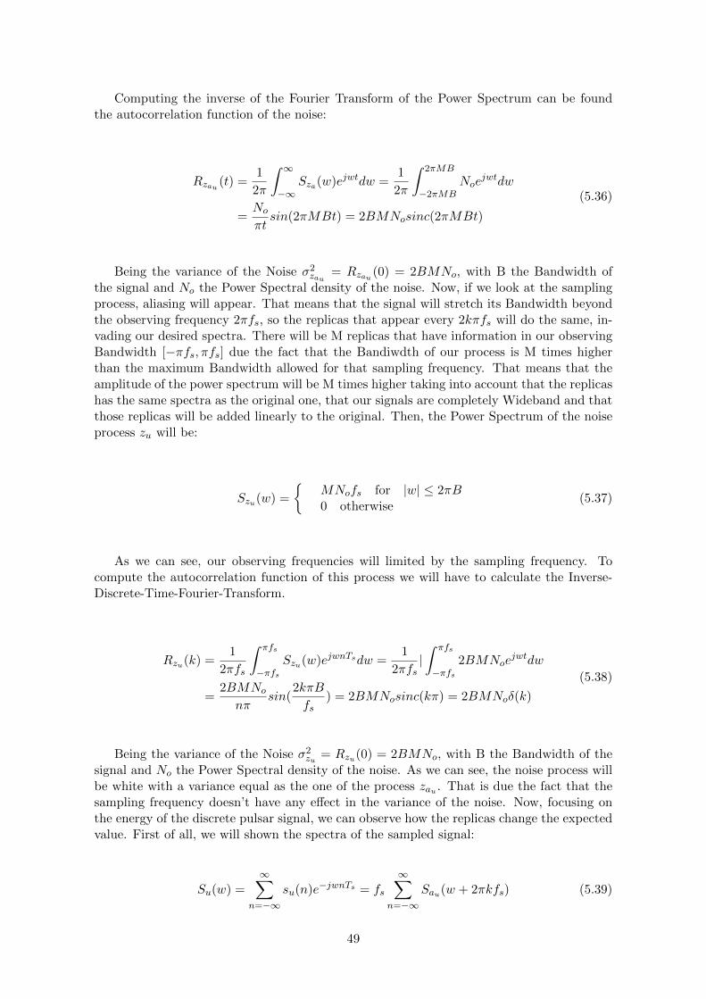
Computing the inverse of the Fourier Transform of the Power Spectrum can be foundthe autocorrelation function of the noise:

Rzau (t) =1

2π

∫ ∞−∞

Sza(w)ejwtdw =1

2π

∫ 2πMB

−2πMBNoe

jwtdw

=No

πtsin(2πMBt) = 2BMNosinc(2πMBt)

(5.36)

Being the variance of the Noise σ2zau

= Rzau (0) = 2BMNo, with B the Bandwidth ofthe signal and No the Power Spectral density of the noise. Now, if we look at the samplingprocess, aliasing will appear. That means that the signal will stretch its Bandwidth beyondthe observing frequency 2πfs, so the replicas that appear every 2kπfs will do the same, in-vading our desired spectra. There will be M replicas that have information in our observingBandwidth [−πfs, πfs] due the fact that the Bandiwdth of our process is M times higherthan the maximum Bandwidth allowed for that sampling frequency. That means that theamplitude of the power spectrum will be M times higher taking into account that the replicashas the same spectra as the original one, that our signals are completely Wideband and thatthose replicas will be added linearly to the original. Then, the Power Spectrum of the noiseprocess zu will be:

Szu(w) =

{MNofs for |w| ≤ 2πB0 otherwise

(5.37)

As we can see, our observing frequencies will limited by the sampling frequency. Tocompute the autocorrelation function of this process we will have to calculate the Inverse-Discrete-Time-Fourier-Transform.

Rzu(k) =1

2πfs

∫ πfs

−πfsSzu(w)ejwnTsdw =

1

2πfs|∫ πfs

−πfs2BMNoe

jwtdw

=2BMNo

nπsin(

2kπB

fs) = 2BMNosinc(kπ) = 2BMNoδ(k)

(5.38)

Being the variance of the Noise σ2zu = Rzu(0) = 2BMNo, with B the Bandwidth of the

signal and No the Power Spectral density of the noise. As we can see, the noise process willbe white with a variance equal as the one of the process zau . That is due the fact that thesampling frequency doesn’t have any effect in the variance of the noise. Now, focusing onthe energy of the discrete pulsar signal, we can observe how the replicas change the expectedvalue. First of all, we will shown the spectra of the sampled signal:

Su(w) =

∞∑n=−∞

su(n)e−jwnTs = fs

∞∑n=−∞

Sau(w + 2πkfs) (5.39)

49

So, taking into account the fact that the signal has a Wideband nature, we know that Midentical replicas will add spectra in our observing frequencies. Furthermore, the spectra ofthe signal is assumed to be almost flat in order to compute easily the energy of su. So wecan find an expression of the energy of the deterministic sampled signal su in comparisonwith the energy of the analogue filtered signal sau as:

εsu =∑n

|su(n)|2

=1

2πfs

∫ 2πfs

0|Su(w)|2dw

=fs2π

∫ 2πfs

0|∞∑

k=−∞Sau(w + 2πkfs)|2dw

∗∗=Mfs2π

∫ πfs

−πfs|Sau(w)|2dw

=Mfs2π

∫ ∞−∞|Sau(w)|2dw

= Mfsεsau

(5.40)

* Taking into account that Sa(w) have contribution of M replicas in w ∈ [−πfs, πfs].

As we can observe, the energy of the sampled signal increase with the sampling frequencyin comparison to the analogue one. This result shows how the energy of the signal is M timeshigher than the one we expected due the fact that the replicas are adding spectral content inour observing frequencies. Now, before computing the ENR and GENR of that process, it isimportant to see the GENR of the signal without undersampling. That means, the GENR ofthe discrete signal of the previous scheme if the sampling frequency was fs = 2BM insteadof fs = 2B . As we know from the other sections, that value will be:

GENR = ENR = εauNo

= MεaNo

As the undersampled noise is white, the ENR will has the same value as the GENR, so:

GENRu = ENRu = εsuσ2zu

=MfsεsauMfsNo

= εauNo

= MεaNo

= GENR

So, different from what we were expecting, undersampling does not change the detectionperformance of the process. That is true if the pulsar signal has a wideband nature and analmost flat spectra. Otherwise, we will have another results. Due the lack of Software, itwill be impossible to perform experiments with an undersampling scheme. However, we canstate that it has no sense to perform it in real applications because that result is only valid ifthe previous assumptions are true. In the reality, the pulsar signal spectrum decreases withthe frequency, so undersampling will slightly decrease the detection performance.

50

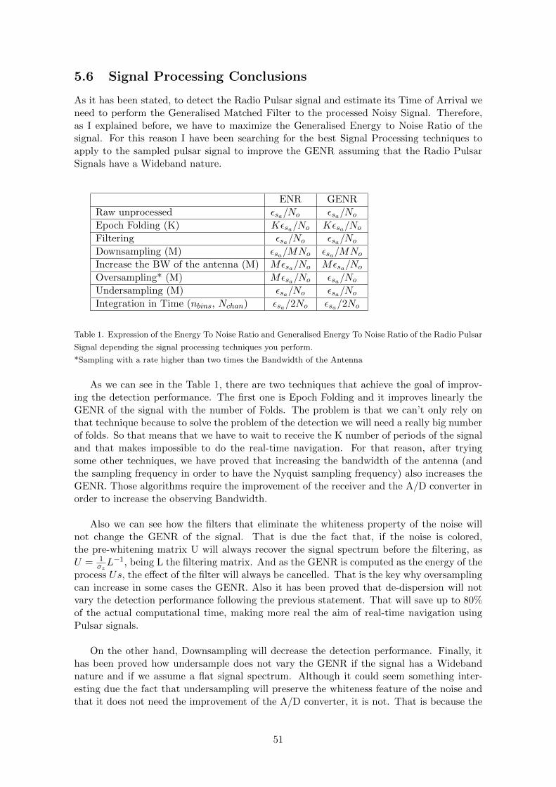
5.6 Signal Processing Conclusions

As it has been stated, to detect the Radio Pulsar signal and estimate its Time of Arrival weneed to perform the Generalised Matched Filter to the processed Noisy Signal. Therefore,as I explained before, we have to maximize the Generalised Energy to Noise Ratio of thesignal. For this reason I have been searching for the best Signal Processing techniques toapply to the sampled pulsar signal to improve the GENR assuming that the Radio PulsarSignals have a Wideband nature.

ENR GENR

Raw unprocessed εsa/No εsa/No

Epoch Folding (K) Kεsa/No Kεsa/No

Filtering εsa/No εsa/No

Downsampling (M) εsa/MNo εsa/MNo

Increase the BW of the antenna (M) Mεsa/No Mεsa/No

Oversampling* (M) Mεsa/No εsa/No

Undersampling (M) εsa/No εsa/No

Integration in Time (nbins, Nchan) εsa/2No εsa/2No

Table 1. Expression of the Energy To Noise Ratio and Generalised Energy To Noise Ratio of the Radio Pulsar

Signal depending the signal processing techniques you perform.

*Sampling with a rate higher than two times the Bandwidth of the Antenna

As we can see in the Table 1, there are two techniques that achieve the goal of improv-ing the detection performance. The first one is Epoch Folding and it improves linearly theGENR of the signal with the number of Folds. The problem is that we can’t only rely onthat technique because to solve the problem of the detection we will need a really big numberof folds. So that means that we have to wait to receive the K number of periods of the signaland that makes impossible to do the real-time navigation. For that reason, after tryingsome other techniques, we have proved that increasing the bandwidth of the antenna (andthe sampling frequency in order to have the Nyquist sampling frequency) also increases theGENR. Those algorithms require the improvement of the receiver and the A/D converter inorder to increase the observing Bandwidth.

Also we can see how the filters that eliminate the whiteness property of the noise willnot change the GENR of the signal. That is due the fact that, if the noise is colored,the pre-whitening matrix U will always recover the signal spectrum before the filtering, asU = 1

σzL−1, being L the filtering matrix. And as the GENR is computed as the energy of the

process Us, the effect of the filter will always be cancelled. That is the key why oversamplingcan increase in some cases the GENR. Also it has been proved that de-dispersion will notvary the detection performance following the previous statement. That will save up to 80%of the actual computational time, making more real the aim of real-time navigation usingPulsar signals.

On the other hand, Downsampling will decrease the detection performance. Finally, ithas been proved how undersample does not vary the GENR if the signal has a Widebandnature and if we assume a flat signal spectrum. Although it could seem something inter-esting due the fact that undersampling will preserve the whiteness feature of the noise andthat it does not need the improvement of the A/D converter, it is not. That is because the

51

real pulsar signal will not have a completely flat spectrum, so the aliasing will not be addedlinearly to the spectrum and the performance will go down. .

Finally, the Integration in Time has been introduced. That technique will reduce thedetection performance. However, it also will highly decrease the number of samples of ourdata. Therefore, Integration in Time may be an interesting technique in order to decreasethe computational complexity of the whole receptor.

52

Chapter 6

Radio Pulsar Signal PSRB0329+54 observations

6.1 PSR B0329+54 features

In order to prove the theoretical background stated in the last chapter, the results of someexperiments with simulated and real data are shown. But, first of all, I will explain thefeatures of the Radio Pulsar signal PSR B0329+54 and the way it has been recorded.

Table 2. Parameters of the Radio Pulsar B0329+54

PSR B0329+54 is a neutron star situated approximately 2,643 light-years away from theEarth in the constellation of Camelopardalis and it was created 6.74 millions of years ago.In 1979, two extrasolar planets were announced to be orbiting the pulsar (being classifiedas pulsar planets). Later observations however ruled out this idea. These radio pulsar emitsone of the strongest polarized pulses received in the north hemisphere with a periodicity of0.71451866398 s. Furthermore, the fact that it has a really low dispersion and an almostnegligible spin down, makes it a good candidate to perform experiments. The DispersionMeasure of that periodic signal is 26.776 cm−3pc, a low enough value that allow us to avoidperforming the de-dispersion process.

Due the intensity of that Radio Pulsar we can make out its pulsar profile after somefoldings. The pulsar has an average flux density at the observation frequency fo = 1400MHz of 203 mJy and an average flux density of 1650 mJy in a fo = 400 MHz. As we canobserve in the next figure, the star has three nested cones of emission and a central coreemission. Also we can see how the pulsar is visible and almost identical in all the observedfrequencies, from 117 MHz to 1170 MHz.

53

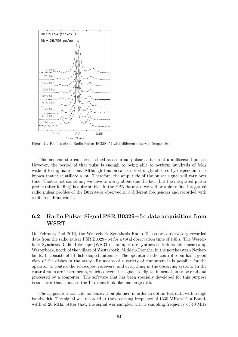
Figure 21. Profiles of the Radio Pulsar B0329+54 with different observed frequencies.

This neutron star can be classified as a normal pulsar as it is not a millisecond pulsar.However, the period of that pulse is enough to being able to perform hundreds of foldswithout losing many time. Although this pulsar is not strongly affected by dispersion, it isknown that it scintillate a lot. Therefore, the amplitude of the pulsar signal will vary overtime. That is not something we have to worry about due the fact that the integrated pulsarprofile (after folding) is quite stable. In the EPN database we will be able to find integratedradio pulsar profiles of the B0329+54 observed in a different frequencies and recorded witha different Bandwidth.

6.2 Radio Pulsar Signal PSR B0329+54 data acquisition fromWSRT

On February 2nd 2012, the Westerbork Synsthesis Radio Telescopes observatory recordeddata from the radio pulsar PSR B0329+54 for a total observation time of 140 s. The Wester-bork Synthesis Radio Telescope (WSRT) is an aperture synthesis interferometer near campWesterbork, north of the village of Westerbork, Midden-Drenthe, in the northeastern Nether-lands. It consists of 14 dish-shaped antennas. The operator in the control room has a goodview of the dishes in the array. By means of a variety of computers it is possible for theoperator to control the telescopes, receivers, and everything in the observing system. In thecontrol room are instruments, which convert the signals to digital information to be read andprocessed by a computer. The software that has been specially developed for this purposeis so clever that it makes the 14 dishes look like one large dish.

The acquisition was a demo observation planned in order to obtain test data with a highbandwidth. The signal was recorded at the observing frequency of 1330 MHz with a Bandi-wdth of 20 MHz. After that, the signal was sampled with a sampling frequency of 40 MHz

54

in order to use the Nyquist sampling frequency and preserve the whiteness property of thereceived noise.

Taking into account the period of the pulsar, 196 complete periods can be extracted fromthe data. This acquisition was stored into 14 files in .dada format with a total weigh of 10.4GB. Each file consists of 4096 bytes of header and then 800000000 bytes of X and Y polar-ization real voltage signal samples interleaved. The format used for each sample is signedinteger with little endian byte ordering: the digital dynamic range goes from -127 to 127,but no information about the amplitude of the voltage signal can be extracted from there.The header contains all the information about the acquisition besides the number of the filebeing open. Each file has 10 seconds of data and the acquisition is consecutive, meaning thatfrom the ending of one file to the beginning of the next no data is lost. The signal is formedas samples of real voltage signals in X and Y polarization interleaved (XYXYXYXYXY).Those signals has been collected by the WSRT with 14 Telescopes. As it has been statedbefore, some beamforming techniques has been applied in the control room in order to haveonly one recorded output signal. The purpose of that is to take profit of the features of theTelescopes of WSRT and to increase the SNR and ENR of the signal with the beamformingtechniques. Apart from that, the sampled voltage signal is not processed in any other way.That means that it is an almost pure, raw signal acquisition.

In the next sections we will assess the GENR of the recorded pulsar signal with the helpof the template taken from the EPN database. That template will allow us to compute thevariance of the noise subtracting the pulsar signal from the acquisition. But before that,some adjustments to the template have to be done in order to have the same amplitude andtime of arrival than the received pulsar signal.

6.2.1 Process to visualize the signal

As I have stated in the last paragraph, we have 14 files .dada with 140 s of recording of thepulsar B0329+54. Taking into account to the period, we can extract 196 complete periodsof that data. However, as we are going to perform Epoch Folding with all those periods,is important to check if the spin down of the pulsar signal will vary our period over time.Before it has been stated that the spin down of the radio pulsar is very small (in the orderof 10−15 ss−1), but not for that reason we have to forget it. In the case we perform EpochFolding over a long time without changing the initial period, we will have a misaligned ofpulsar signals added together in the wrong position. That will lead to a bad performance ofEpoch Folding and a change of the pulsar profile. As we do not want that to happen duethe fact that we need a clean pulsar profile to perform the Matched Filter, we are going tocheck the true period of the pulsar signal.

[17] explains the procedure to calculate the correct period of the Radio Pulsar Signaldepending on how many folds you perform. During the first folds the Ptrue will be almostthe same as the original period. But, after 50 folds the folded signal start drifting to theright, the profile starts to broaden and the pulsar signal profile starts to blur. So, as wecan see in [17], the correct period for 196 foldings should be Ptrue = 0.7145579 s and thenumber of samples per period will be 28582316. That change in the period will be a problemin order to read the data. The initial data has been recorded in order to have a period of0.71451866398 s. So, in every file there are 14 exact periods of 28580746 samples. Now, if wechange the length of the periods, we will have to split the reading of the 14th period of everyfile in two steps. Finally, that will provoke to have 195 whole periods in all the recordeddata, having to left without reading a little portion of the 196th period. Although it look

55

like a problem, at the end we will see as the final folded pulsar profile will be very accurate.

First, the two polarized voltage shas been integrated in order to have the pulsar powerprofile. To do that, both voltages signal will be combined in this way:

Pprofile = |Vx|2 + |Vx|2

That profile will be a signal with a range of values between [0,16128]. As it is verycomplex from a computational point of view to work with a signal with 195 periods, wewill perform the next techniques to one period. So, in case we want to perform the EpochFolding, that will be the moment. That is to say, if we want to perform Epoch Folding, wewill perform it in this part of the process to adequate the signal. So, from now on, our signalwill be modelled as:

y(n) = s(n) + z(n)

Being s the pulsar signal and z Additive White Gaussian noise with unknown mean overone period. Although is not something critic, it will be clearer to work with the exact meanof the radio pulsar signal, so we have to find the mean of the process y. To do that, we haveto take into account that the received noise process have 0 mean, so the mean of the totalsignal will be:

E(y) = E(s+ z) = E(s) + E(z) = E(s)

Hence, we need to know the mean of the radio pulsar signal in order to compute themean of the whole process. To do that, we need to use the template of the pulsar signalB0329+54 taken from the EPN database. That template is a signal with 1024 samples withan amplitude A and a time of arrival τ . In order to know the exact amplitude, and therefore,the mean of the received signal, first we have to estimate the values of the amplitude andtime of arrival of the template. Furthermore, as our signal y have 28582316 samples, firstwe have to upsample the template. The next step was estimating the time of arrival of theradio pulsar signal. As it has been stated in the detection theory, the best way to do it isperforming N matched filters of the templates and the radio pulsar signal and see in whatposition the value is maximum. After doing that, it was clear that the signal was shifted335000 samples, so I shifted the template that number of samples to being able to computethe better ENR possible. The last step to being able to have the real mean of the signalwas estimating the amplitude of the radio pulsar received signal. As stated in the detectiontheory, the value of the MLE of the amplitude will be a = <y,p>

<p,p>

With that processes, we can state that the resulting template p is the best estimation ofthe received pulsar. This process has to be repeated if we use a folded signal or if we changethe number of foldings. The time of arrival will not vary with the folding, though, so we donot have to compute again the matched filter. So, if instead of working with the unprocessedsignal we start working with a K folded signal, we have to estimate the amplitude of thetemplate again.

56

From now on, we can visualize and work with the signal y and the template p. In thenext section I will show the visualization of the radio pulsar signal, as well as compute theamplitude, mean, energy of the pulsar signal, the variance and spectra of the noise and theENR of the whole process.

6.2.2 Representation of the radio Pulsar Signal

In this section I am going to show the plots and the features of the radio pulsar signalB0329+54 described before. First of all, we are going to assume that our unprocessed signalis y = s+z, being s the pulsar signal and z the Additive White Gaussian Noise. Also we havethe Template p, with the same time of arrival, shape and amplitude as the received pulsarsignal. The process described in the last sections have been performed in this template inorder to have a replica of the received pulsar signal. So, we can state that p = s. Therefore,the GENR and ENR of the process can be assessed. In fact, the value of the GENR willbe the same as the ENR due the fact that the noise is white. We will see that in the nextfigures, where the Power Spectrum of the noise process will be shown. So, finally we can seeas the GENR:

GENR = ENR = 39.9dB

In the next figure we can observe the plots of the noisy signal and the Template in thetime domain.

F igure 22. Representation of the unprocessed noisy pulsar signal (left) and the radio pulsar signal Tem-

plate (right).

From that unprocessed noisy pulsar signal we can see as the radio pulsar signal is com-pletely submerged in noise. Moreover, there are 4 interference with a big amplitude thathas not interest. As we will see in the results of the experiments in the Chapter 7, thoseinterference will disappear with the performance of the Epoch Folding technique. Then, ifwe look at the Template we can see as the estimating amplitude is around 30 while themaximum amplitude of the noise is about 2000. That shows how small are the unprocessedpulsar signal if we compare it with the noise. If we keep looking to the template, we can

57

see the power pulsar profile, and how it has the same features that have been described inthe last sections. Now, after looking the signal in the time domain, the power spectrum ofthe noise process z and the noisy signal y is computed in order to see the frequency domaincharacteristics. Due to the fact that with Matlab is difficult to show the real spectrum ofthe signal, I am going to compute the power spectrum of the real data. To compute it, theperiodogram approximation is used:

1) Compute the FFT of the time-domain signal and take the absolute value

2) Divide it by the square root of the number of samples

3) Apply an average filter

4) Do the square of the filtered signal

Finally, we have 1L |Sxx(f)|2, being Sxx the average FFT of the signal s. This is a good

approximation of the power spectrum, and therefore, of the spectrum of the signal. First ofall, I will show the noise spectrum in order to see the whiteness property and the value ofthe power spectral density.

Figure 23. Representation of the Power Spectrum of the unprocessed noise.

Looking at the Figure 23 we can take some conclusions. The first one is that, as we wereexpecting, the noise power spectrum is completely flat, so the unprocessed noise process iswhite. However, we can see a small peak in the center of the spectrum due the little differ-ence between the Template and the Real Pulsar Signal. That is because the noise have beencomputed as y − p = y − s = z, so any small difference between the real pulsar signal andthe template will be reflect in the noise power spectrum. Anyway, this little interference isnegligible in the computation of the variance of the noise. Another conclusion we can observeis the fact that the amplitude of the power spectrum is equal to the variance of the noise.That proves the fact that the power spectrum of the white sampled noise is fsNo, exactlythe same value as the variance if the noise is white. Now, the power spectrum of the whole

58

signal is shown in order to see if the signal is wideband as we are expecting. Computing itwith the same process as the used for the noise power spectrum, we have:

Figure 24. Representation of the Power Spectrum of the Radio Pulsar noisy signal.

Looking carefully at the figure 24, we can see as the bandwidth of the pulsar signal is 200Hz and with an amplitude higher than the noise spectrum . So, the signal received from theWSRT looks very narrowband. That result is the opposite that the one we were expectingdue the fact that the radio pulsar signals has a wideband nature. Moreover, looking at thosekind of Bandwidth (the order of MHz) we should see an almost completely flat spectrum.From this figure we cannot still conclude that the radio pulsar signal recorded by the WSRThas a narrowband nature because we are looking at the power spectrum of the signal andnot the real spectrum. However, I will prove in the Chapter 7 the fact that the pulsar signalfrom the WSRT has an almost narrowband nature.

59

Chapter 7

Signal Processing experiments

In this section, experiments proving the performance of the algorithms explained in the Chap-ter 5 with Wideband Signals submerged in Additive White Gaussian Noise will be shown. Todo that, I am going to divide it in two subsection. First, I will perform simulations with fakedata created by Matlab. In that part I am going to prove that the GENR of the WidebandSignal increases when you perform Epoch Folding and when you improve the bandwidth ofthe receiver. As stated in Detection Theory, increasing the GENR will mean increasing thedetection performance and the estimation of the Time Of Arrival of the Wideband Signal.Furthermore, I will show that Low-Pass filtering doesn’t change the detection performanceand that it decreases with Downsampling.

After that, I will perform the same algorithms to a Real Radio Pulsar Signal PSRB0329+54 provided by the Westerbork Synthesis Telescope. We will see as the results withthat real data will not be the ones we are expecting. I am going to provide an explanationof those results.

7.1 Simulated data

In that subsection we are going explained how I have created a Wideband Fake Radio PulsarSignal submerged in white noise to apply the 5 algorithms explained in that report. Af-ter that, we are going to assess the ENR and GENR to the signal after every processingstep to prove the theory stated before. The data has been implemented with Matlab. Fur-thermore, the other signal processing techniques also has been performed with that Software.

First of all, it has been created a simulated data with features similar to a Radio Pulsarsignal s with length of 2000 samples and a bandwidth of 10 kHz. The simulated data thatreach the properties of the star pulses (Wideband, Time-Limited and accurate periodicity)is the Additive White Gaussian Noise with a duration of few samples. In this case, a AWGNsignal of length 100 samples over a 2000 samples background has been implemented with anenergy of εs = 1.01 ∗ 106. The fact that this fake pulsar signal is an additive white gaus-sian noise makes the spectrum Wideband. Moreover, the spectrum is almost flat, importantproperty to show the linear improvement of the GENR of the signal after applying the signalprocessing techniques. In the next figure we can observe the fake rotating star sampled pulsein the time domain.

60

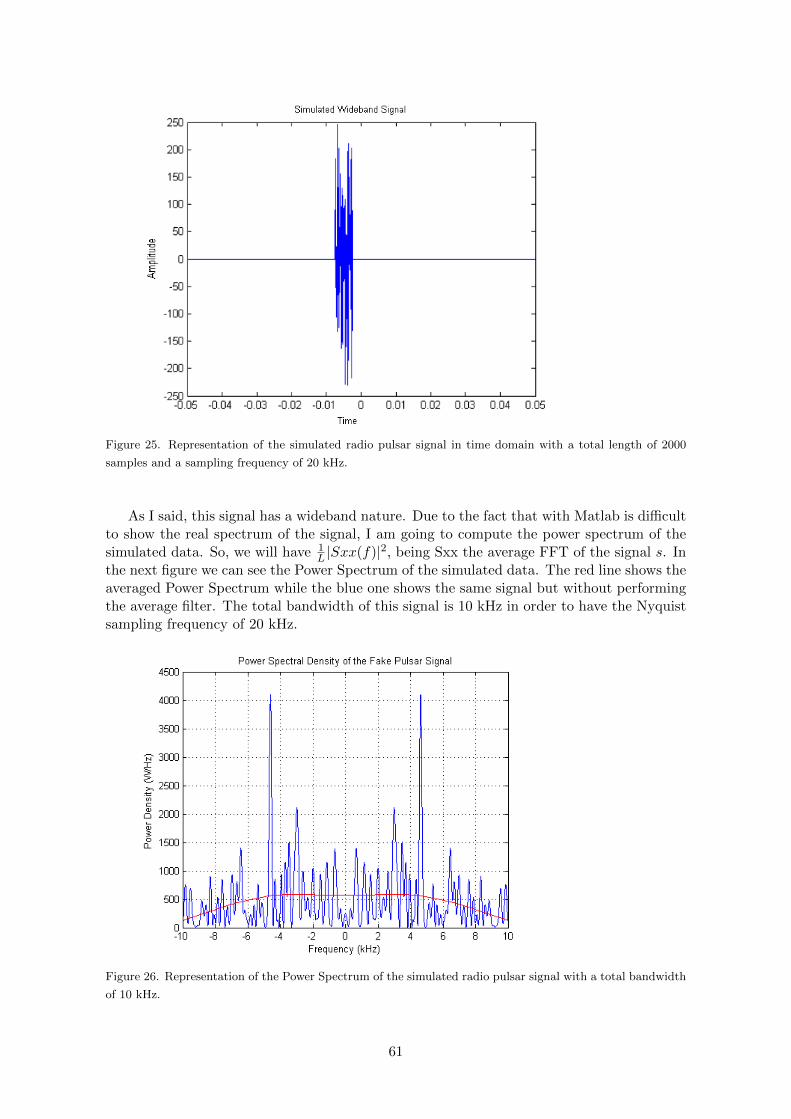
Figure 25. Representation of the simulated radio pulsar signal in time domain with a total length of 2000

samples and a sampling frequency of 20 kHz.

As I said, this signal has a wideband nature. Due to the fact that with Matlab is difficultto show the real spectrum of the signal, I am going to compute the power spectrum of thesimulated data. So, we will have 1

L |Sxx(f)|2, being Sxx the average FFT of the signal s. Inthe next figure we can see the Power Spectrum of the simulated data. The red line shows theaveraged Power Spectrum while the blue one shows the same signal but without performingthe average filter. The total bandwidth of this signal is 10 kHz in order to have the Nyquistsampling frequency of 20 kHz.

Figure 26. Representation of the Power Spectrum of the simulated radio pulsar signal with a total bandwidth

of 10 kHz.

61

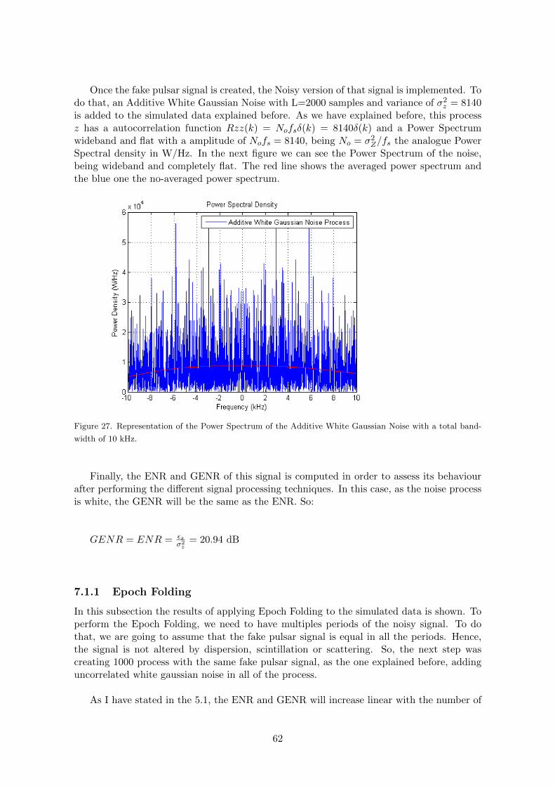
Once the fake pulsar signal is created, the Noisy version of that signal is implemented. Todo that, an Additive White Gaussian Noise with L=2000 samples and variance of σ2

z = 8140is added to the simulated data explained before. As we have explained before, this processz has a autocorrelation function Rzz(k) = Nofsδ(k) = 8140δ(k) and a Power Spectrumwideband and flat with a amplitude of Nofs = 8140, being No = σ2

Z/fs the analogue PowerSpectral density in W/Hz. In the next figure we can see the Power Spectrum of the noise,being wideband and completely flat. The red line shows the averaged power spectrum andthe blue one the no-averaged power spectrum.

Figure 27. Representation of the Power Spectrum of the Additive White Gaussian Noise with a total band-

width of 10 kHz.

Finally, the ENR and GENR of this signal is computed in order to assess its behaviourafter performing the different signal processing techniques. In this case, as the noise processis white, the GENR will be the same as the ENR. So:

GENR = ENR = εsσ2z

= 20.94 dB

7.1.1 Epoch Folding

In this subsection the results of applying Epoch Folding to the simulated data is shown. Toperform the Epoch Folding, we need to have multiples periods of the noisy signal. To dothat, we are going to assume that the fake pulsar signal is equal in all the periods. Hence,the signal is not altered by dispersion, scintillation or scattering. So, the next step wascreating 1000 process with the same fake pulsar signal, as the one explained before, addinguncorrelated white gaussian noise in all of the process.

As I have stated in the 5.1, the ENR and GENR will increase linear with the number of

62

folds once you perform the folding. Therefore, the improvement of the Generalised Energyto Noise Ratio is:

GENRK = ENRK = εsσ2zK

= Kεsσ2z

Being the GENR equal to the ENR because of the Epoch Folding doesn’t change thewhiteness property of the noise process z. In the next Figures we can observe how the EpochFolding increase linearly the detection performance in the lineal domain and in a logarithmicway in the log domain.

F igure 28. Representation of the Generalised Energy To Noise Ratio for a different number of Folds in

the linear (left) and logarithmic domain (right).

As we can observe, the results of the experiments are the ones we were expecting. More-over, as the Epoch Folding also increases the Signal to Noise Ratio, so we will be able to seethe effects of the folding looking to the signals. In the Figure 29 we can see the unprocessednoisy signal and the same signal after adding 1000 periods together. Is really easy to observehow the noise is almost gone although the fake pulsar signal is not altered.

63

F igure 29. Representation of the unprocessed noisy simulated data (left) and the same signal after ap-

plying epoch folding with K=1000 (right).

As it can be observed, after K = 1000 folds the GENR and therefore, the ENR hasincreased 30 dB, exactly the value we were expecting.

That section proves that Epoch Folding increase the detection performance of the signal,so it will be useful to use it to the real pulsar to increase the performance of the real-timenavigation.

7.1.2 Low-Pass Filtering

After proving that Epoch Folding increases linear the detection performance, in this sectionit will be proved that Low-Pass Filtering the Pulsar Signal will not alter the the GENR. Atthe end we concluded that:

GENRf = pTΦ−1v p = εUp

=∑n

| 1

σzs|2 =

εsσ2z

= GENR

(7.1)

Being p the low-pass filtered version of the pulsar signal s, and v the low-pass filteredprocess of z. So, the GENR of the Low-pass Filtered signal should be the same as the GENRof the unprocessed noisy pulse.

To perform that experiment I took the simulated signal y = s + z = p1 + v1 of 2000samples with a sampling frequency of 20 kHz and a Bandwidth of 10 kHz as the signalfiltered by a low pass filter with cut-off frequency fc = B/M = 10/M kHz with M = 1. Thenext step was creating the low pass filter with a different cut-off frequencies, and therefore,different values of M. The filter has been made in order to be able to perform the inverse ofthe filtering matrix without eigenvalues problems. Hence, to be able to compute the inverse

64

covariance of the filtered noise. To deal with that problem explained in 5.2, I have createda filter with a non-zero spectrum, being 0.1 outside the band-pass zone.

After that, I have performed the filtering with different values of M until a maximumvalue of M = 10. Therefore, the resultant filtered signal is yfM = p + v = Ls + Lz withL the filtering matrix. In order to do compute the GENR of the processes yfM , the covari-ance matrix of the filtered noise v is needed. There are two ways of computing it with Matlab:

1) As I said in 5.2, the covariance matrix of the filtered noise is Φv = E(vvT ) =E(LzzTLT ) = LΦzL

T = σ2zLL

T . So, as we know the value of the σ2z , computing the

Filtering Matrix L we will be able to have the covariance matrix of the filtered noise. So,doing the inversion of this matrix, we will have the Φ−1

v .

2) The second method is an approximation. As we cannot compute the expected valueof the noise process, we are going to taking into account the law of the large numbers. Thislaw states that the average of N trials, with N big, should be close to the expected value ofthat process. Mathematically can be seen as:

P (| 1N

∑N

vvT − E(vvT )| < ε) ≥ 1− σ2

Nε2(7.2)

Being σ2 the variance of the process zzT , ε a value as small as you want and N thenumber of experiments done. As we can see, for a large N, the probability of the averagebeing equal as the expected value is almost 1. In order to have a good approximation, theN should be larger than 10 times the length of the signals.

In that experiment I have computed the covariance matrix doing N = 20000 independentexperiments of the processes vMv

TM . Then, I have performed the inverse of those covariance

matrix. Finally, we are able to asses the GENR = pTΦ−1v p to every low pass filtered process.

In the next Figure we can see the values of the GENR of the filtered signal while we increaseM.

65

Figure 30. Representation of the GENR of the low-pass filtered signal depending on the M, with M = B/fc

or fc = B/M .

As we can observe, the GENR doesn’t change with the different cut-off frequencies. Thatproves the theoretical fact that Low-Pass Filtering a radio pulsar signal doesn’t change thedetection performance.

7.1.3 Whitening Process

Before assessing the GENR and ENR of the signals after performing downsampling, I amgoing to show some results of the whitening processes used in the Low-Pass Filtering exper-iments. In the last section we have seen as the processs U and p, being U the whiteningmatrix and p the filtered signal, can be written as:

U = 1σzL−1

p = Ls

v = Lz

Where s and z are the signal and noise processes before applying the Low-pass filter L.So, in order to assess the GENR of the filtered signal, we have to compute the energy of theprocess Up. As stated before, Up = 1

σzL−1Ls = s

σz. That equation shows how the whitening

matrix is recovering the high frequencies of the signal p cutted by the Low-pass filter. Thatmeans that the matrix U and the signal p do not forget completely the shape and the valuesof the high frequencies of the signal s once you have performed the filter.

That assumption can be questioned with the argument that the high frequencies havebeen eliminated by the filter, so it is impossible to recover them in the total spectrum. Also,as the whitening matrix doesn’t depend on the shape of the signal, is difficult to believethe total reconstruction. The point is that the filtered signal p although it has not high

66

frequencies, it keeps remembering them. We can see that in the expression p = Ls. So, theconclusion will be that the inverse of the filtering matrix L−1 perform the role of a recon-struction filter.

To prove that, I checked the Power spectrum of the process Up, being p the low-passfiltered signal with a cut-off frequency fc = B/2. But first of all, the Power Spectrums ofthe unprocessed signal s and the low-pass filtered signal p are shown.

F igure 31. Representation of the Power Spectrum of the unprocessed signal s (left) and the Power Spec-

trum of the low-pass filtered signal p (right).

We can see as the signal p has a bandiwdth of 5 kHz due to the application of the Low-Pass filter. The next step was computing the whitening matrix U and create the new processUp. The energy of this process will be the value of the GENR of the filtered signal. In thenext figure we can observe the Power Spectrum of that process.

Figure 32. Representation of the Power Spectrum of the process Up, being U the whitening matrix taken

from the inverse of the filtered noise covariance matrix and p the Low-pass filtered signal.

67

Looking at the Figure 32 we can state that the whitening matrix is recovering the highfrequencies of the signal s, eliminated by the filter. Also we can observe that the amplitudehas decreased in σ2

z . That is due the whitening process have a normalization by a factor σ2z ,

the variance of the noise before applying the filter.

7.1.4 Downsampling

In that section we are going to assess the GENR when you downsample a signal. To do iteasier, I am going to perform the downsampling to the simulated noisy signal of L = 2000with the same factors M as the ones in the Low-Pass Filtering experiment. In the chapter5.3 I have concluded that downsampling decreases the ENR and the GENR by a factor ofM . Hence, the detection performance is decreased.

So, if we take into account that yd = r + W , being yd the downsampled noisy signal, rthe fake downsampled pulsar signal and W the downsampled noise process, the ENR of the

downsampling signal will be ENRd = εr/σ2W = εs

M2 /σ2zM = ENR/M . Moreover, as the noise

process z is Additive White Gaussian Noise, the downsampling will not change the whitefeature on the process W . Therefore, the value of the GENR will be the same as the valueof ENR.

Figure 33. Representation of the Generalised Energy To Noise Ratio for a different values of the downsam-

pling factor M in the linear domain

As we were expecting, the detection performance decrease when M increases. Is not de-creasing in a linear way because the spectrum of the simulated pulsar signal is not completelyflat. Moreover, as we are looking at signals with a length up to 200 samples, the accuracyof the ratios in not perfect. However, if you look carefully, the value of the GENR is around10 when M = 10 and around 120 when M = 1, so the decrement is almost lineal.

68

7.1.5 Increase the Bandwidth of the signal

In the last section it has been concluded that decreasing the Bandwidth of the receiver/antennadecreases the ENR, GENR and the detection performance. So, we can demonstrate that in-creasing the Bandwidth of the antenna improves the detection performance knowing thatthe opposite technique, downsampling, decrease the GENR. Anyway, in this section I willshow the results of how increasing the Bandwidth of the signal, and therefore, the samplesper period, improve the ratios used in this Thesis.

Before showing the result of the experiments done with simulated data, first I will sumup the theory of how increasing the Bandwidth of the receiver/antenna improves the GENR.If we take a look at the next figure, we can see the schemes of both cases. The one with aBandwidth B and the one with a Bandwidth MB. The sampling frequency will always bethe Nyquist one. Hence, two times the Bandwidth of the signal.

F igure 34. Representation of the receiver scheme of the signal with a Bandwidth B Hz (left) and the one

with the signal with a Bandwidth MB Hz (right).

As we can observe, the analogue Low-Pass filter will not change anything as its cut-offfrequency is the same as the Bandwidth of the antenna. However, it is shown in order toeliminate the spurious. Looking at the left figure, we can see as is the same scheme as theunprocessed signal shown in the chapter 4. Therefore, we know that the ENR and the GENRof that signal will be:

GENR = ENR = εsaNo

Now, looking at the second Scheme, we can see as the energy of the signal saM will be Mtimes higher than the energy of sa due it has M times more Bandwidth. In addition, as thesampling frequency is also M times bigger in the second scheme, the energy also will increasein a factor M . So, finally we can state that:

εsM = fsoεsaM = MfsεsaM = M2fsεsa

The noise process zM though, only will increase its variance in a factor of M if we com-pare to the noise process z. That is due the fact that the A/D converter doesn’t increasethe variance of the noise no matter the sampling frequency used. Then, it will be increasedby M due the bigger Bandwidth of zM . So, the variance of the noise process zM will be:

69

σ2zM

= Mσ2z = MfsNo

Finally, and taking into account that the process zM is white with autocorrelation func-tion RzM (k) = 2MBNoδ(k), the GENR will be:

GENR = ENR =εsMσz2M

= M2fsεsaMfsNo

= MεsaNo

So, it can be seen as the GENR is increased by a factor of M. Now, to prove that I willshow the results of the experiments done. First of all we will consider the signal without theBandwidth increased. That will be a simulated signal with Bandiwdth 1 kHz, a samplingfrequency of 2 kHz and length 200 samples. Then, it has been created the signals with thesame properties but with a increased Bandwidth. The new signals will have a Bandwidth ofB = M kHz with a sampling frequency of 2M kHz and length 200M samples. To do thatexperiment, it has been chosen different values of M between 1 and 10, being the signal withM = 10 the one I have shown in the section 7.1.1. So, after computing the GENR of thedifferent signals, we can see the evolution of it with the increment of M.

Figure 35. Representation of the Generalised Energy To Noise Ratio for a different values of M. Being M the

factor of increment of Bandwidth

Looking at the figure 35 we can see how increasing the Bandwidth of the receiver im-proves in a linear way the GENR. Hence, the detection performance will also be increased.The improvement is not completely linear due the fact I have done the simulations withsignals of few samples, so the accuracy of the process is not perfect. Anyway, it can be easilyseen as the ratio is improved.

70

7.2 Radio Pulsar signal B0329+54 from WSRT

In that section I will show the results of the experiments with the Real Radio Pulsar Signaldata from the Westerbork Synthesis Radio Telescope. The problem is that this pulsar looksbehave like a narrowband signal, defying its wideband nature. However, only observing thepower Spectrum of the real data we cannot conclude that the pulsar signal data is narrow-band due the fact that the Power spectrum we compute is not the same as the real spectrumof the signal. So, the experiments done in this subsection will be shown in order to provethe ”narrowband” nature of this recorded pulsar signal. The experiments done to the realdata has been:

1) Epoch Folding, in order to see how this technique increase the SNR and GENR nomatter the spectrum of the signal. Also to being able to see the blurred pulsar profile andhow it dissapear after performing a High-Pass Filter.

2) Downsample the signal to see how the SNR of the signal is improved and the GENRis not changed. In fact, a downsampling by a factor of 27885 has been performed in orderto see how the noise disappear and only the signal remains. Finally, a high pass filter willprove the almost narrowband nature of the pulsar signal taken from the WSRT.

3) Integration in Time, in order to see the Pulsar Profile for every frequency channel.We will see as the shape of the pulsar can be seen for a high frequencies although reallyattenuated. So, the behaviour of the pulsar is closer to a Narrowband signal.

7.2.1 Epoch Folding + High Pass Filter

First of all, I performed the Epoch Folding with different values of K in order to assess theGENR. The periods have been added every 28582316 samples. This number of samples isused in order to perform the Epoch Folding with the new period computed in the section6.2.2. In the next figure we can observe the evolution of the GENR of the signal dependingthe number of folds. The assessment of the ratios has been done every 14 folds, finishingwith K=195. The results we are expecting is an improvement of 10log(195) = 22.90dB inboth ratios.

71

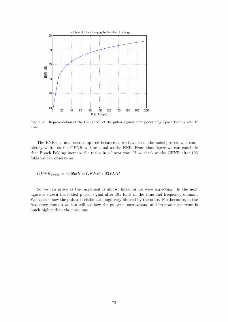
Figure 36. Representation of the the GENR of the pulsar signals after performing Epoch Folding with K

folds.

The ENR has not been computed because as we have seen, the noise process z is com-pletely white, so the GENR will be equal as the ENR. From that figure we can concludethat Epoch Folding increase the ratios in a linear way. If we check at the GENR after 195folds we can observe as:

GENRk=195 = 62.95dB = GENR+ 23.05dB

So we can prove as the increment is almost linear as we were expecting. In the nextfigure is shown the folded pulsar signal after 195 folds in the time and frequency domain.We can see how the pulsar is visible although very blurred by the noise. Furthermore, in thefrequency domain we can still see how the pulsar is narrowband and its power spectrum ismuch higher than the noise one.

72

F igure 37. Representation of the Folded Radio pulsar signal after 195 folds in time domain (left) and in

the frequency domain (Power Spectrum)(right)

We can observe as the signal is still narrowband with a Bandwidth of 200 Hz after thefolding. From now on, to make easy and intuitive the experiments we are going to work withthe Folded signal.

After showing the effects of Epoch Folding , a high-pass filter with a cut-off frequencyof 80 kHz has been performed in order to show how the pulsar signal of the Figure 37 dis-appear. To start with the experiment, first it has been created a High-Pass Filter h(n) withthe Software Matlab. The filter have has an amplitude of 1 in the frequencies between 80kHz and 20 MHz and almost 0 from 0 Hz to 800 kHz. The next figure shows the transferfunction of this filter.

Figure 38. Representation of the frequency response of the High-Pass Filter created with Matlab.

73

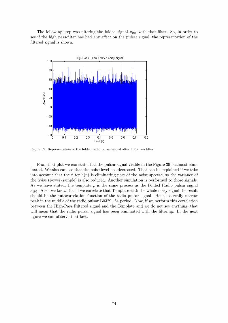
The following step was filtering the folded signal y195 with that filter. So, in order tosee if the high pass-filter has had any effect on the pulsar signal, the representation of thefiltered signal is shown.

Figure 39. Representation of the folded radio pulsar signal after high-pass filter.

From that plot we can state that the pulsar signal visible in the Figure 39 is almost elim-inated. We also can see that the noise level has decreased. That can be explained if we takeinto account that the filter h(n) is eliminating part of the noise spectra, so the variance ofthe noise (power/sample) is also reduced. Another simulation is performed to those signals.As we have stated, the template p is the same process as the Folded Radio pulsar signals195. Also, we know that if we correlate that Template with the whole noisy signal the resultshould be the autocorrelation function of the radio pulsar signal. Hence, a really narrowpeak in the middle of the radio pulsar B0329+54 period. Now, if we perform this correlationbetween the High-Pass Filtered signal and the Template and we do not see anything, thatwill mean that the radio pulsar signal has been eliminated with the filtering. In the nextfigure we can observe that fact.

74

F igure 40. Representation of the correlation between the folded signal and the Template (left) and cor-

relation between the folded signal after high pass filter it and the Template(right)

The correlation between the high-pass filtered signal and the template is almost 0. Thatmeans that the signal does not have nothing in common with the template.

7.2.2 Downsampling + High-Pass Filter

In this section it is showed the performance of Downsampling to the folded signal y195 by afactor of 27885. That is done in order to obtain a resultant signal with 1025 samples. Alsoit has been done to compute the extreme case when the signal is low-pass filtered with acut-off frequency of 717 Hz. In the next Figure we can see the Downsampled pulsar signalin the time domain.

Figure 41. Representation of the folded radio pulsar signal after downsampled it by 27885.

75

The Figure shows the pulsar power profile with the same level as the template beforeDownsampling. That means that the Low-Pass filter is not cutting any spectra of the pulsarsignal. With that result we can take two conclusions. First, the low-pass filter is not de-creasing the energy of the pulsar signal. The second is that the estimation of the amplitudeof the template is really accurate.

Now, if we compute the SNR of that downsampled signal we can see as SNR = 24.60dB.That means that the SNR has increased in 36.2 dB, where it should be 0 dB if the signalhad a wideband nature. Finally, the a high-pass filter has been applied in order to see howthe Radio Pulsar Signal is almost eliminated. First, we have to take intro account that thedownsampled signal will have a Bandwidth of 717 Hz and a sampling frequency of 1434 Hz.So, the cut-off frequency of the high pass filter is fc = 250Hz. In the next figure we can seethe downsampled process after high pass filter it. As it can be observed, the signal has beenalmost eliminated by the filter, another prove that the data from WSRT has been storedeliminating its wideband feature.

Figure 42. Representation of the downsampled radio pulsar signal after high-pass filter it.

7.2.3 Integration in Time

The final experiment has been the Integration in Time separating the signal in 33 frequencychannels. Doing that we will be able to see the Integrated Pulsar Profile of the signal for adifferent frequencies. The channel 1 shows the lowest frequencies and the channel 33 showsthe highest ones. In the next figure we can see the Power Pulsar Profile without noise in thefirst channel. That is due the fact that Integration on time highly increases the SNR of thesignal.

76

Figure 43. Representation of the Power Pulsar Profile in the first Frequency Channel (of 33).

The most important thing of that figure in order to check if the received signal is nar-rowband is the amplitude. If the data behave as a real Pulsar, the other frequency channelsshould show the same Pulsar Power Profile with almost the same amplitude. This is due thefact that Radio Pulsar Signals are really Wideband, so the intensity of the pulsar should notvary in a observation Bandwidth of 20 MHz. In the next figure we can see the Pulsar Profilefor the 4th frequency channel.

Figure 44. Representation of the Power Pulsar Profile in the fourth Frequency Channel (of 33).

We can see as the Pulsar Profile can still be observed but with a lot of noise. Furthermore,

77

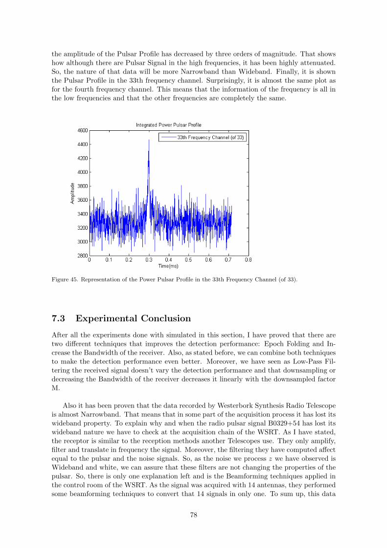
the amplitude of the Pulsar Profile has decreased by three orders of magnitude. That showshow although there are Pulsar Signal in the high frequencies, it has been highly attenuated.So, the nature of that data will be more Narrowband than Wideband. Finally, it is shownthe Pulsar Profile in the 33th frequency channel. Surprisingly, it is almost the same plot asfor the fourth frequency channel. This means that the information of the frequency is all inthe low frequencies and that the other frequencies are completely the same.

Figure 45. Representation of the Power Pulsar Profile in the 33th Frequency Channel (of 33).

7.3 Experimental Conclusion

After all the experiments done with simulated in this section, I have proved that there aretwo different techniques that improves the detection performance: Epoch Folding and In-crease the Bandwidth of the receiver. Also, as stated before, we can combine both techniquesto make the detection performance even better. Moreover, we have seen as Low-Pass Fil-tering the received signal doesn’t vary the detection performance and that downsampling ordecreasing the Bandwidth of the receiver decreases it linearly with the downsampled factorM.

Also it has been proven that the data recorded by Westerbork Synthesis Radio Telescopeis almost Narrowband. That means that in some part of the acquisition process it has lost itswideband property. To explain why and when the radio pulsar signal B0329+54 has lost itswideband nature we have to check at the acquisition chain of the WSRT. As I have stated,the receptor is similar to the reception methods another Telescopes use. They only amplify,filter and translate in frequency the signal. Moreover, the filtering they have computed affectequal to the pulsar and the noise signals. So, as the noise we process z we have observed isWideband and white, we can assure that these filters are not changing the properties of thepulsar. So, there is only one explanation left and is the Beamforming techniques applied inthe control room of the WSRT. As the signal was acquired with 14 antennas, they performedsome beamforming techniques to convert that 14 signals in only one. To sum up, this data

78

cannot be used to prove the signal processing theoretical techniques explained to improve thedetection of the radio pulsar signal. Besides, it is not recommendable to use it for detectionapplications since the narrowband nature of this rotating star pulse makes impossible toimprove the detection with the basic signal processing techniques. That is due the fact thatnot any applications we have introduced in this Thesis improves the GENR of the pulsarsignal if it is narrowband.

79

Chapter 8

Proposed Receptor

After all the things stated during the Thesis I am going to introduce the optimum receptor todetect the Radio Pulsar signals and estimate its time of arrival. In order to assure that thisreceptor is the best for this application we have to assume that the pulsar signal is Wideband.

In the section 3 we have concluded that the best way to detect a signal submergedin Additive White Gaussian Noise is the GLRT detector. That detector can perform thesub-optimum detection performance for a given false alarm probability. Moreover, the imple-mentation of the GLRT detector is N correlations with N shifted Templates (with differentshifts). The shift that gives the highest correlation value will be our estimation. This τ willbe the best estimation of the time of arrival of the signal. Then, if that correlation value isabove a threshold, we will assume that we have detected the signal. So, the probability ofdetection of the pulsar after performing the Generalised Matched Filter is:

Pd = Q(P−1(PFA)−√sTΦ−1

z s) = Q(P−1(PFA)−√GENR)

∗= Q(P−1(PFA)−

√εsσ2z)

* Assuming that the noise is white, so the GENR will have the same value as the ENR.

Looking at the last expression, we can state that in order to improve the detection per-formance for a given false-alarm probability we have to increase the ENR (GENR for colorednoise) of the signal before applying the detector as much as you can. As the estimation of thetime of arrival is related to the probability of detection, we can state that the improvement ofENR also will increase the estimation performance and therefore, the feasibility of creatinga real-time navigation using radio pulsar signals. In fact, in the simulations performed byDr. Richard Heusdens in [1] we can observe that the time of arrival is estimated in a correctway for a ENR of 16 dB. That value will give us a limit in the increment of the ENR, soonce we achieve that value the goal will be to reduce as much as possible the processing timerequired to detect the signal.

To sum up, in this Thesis has been explained two cases when the GENR of the signal isimproved. The first one has been the Epoch Folding, where we average the received pulsarsignals taking into account the period of the pulsar. But, if we want to perform a real-timenavigation we cannot lose too much time waiting for the signals to arrive. Then, the bestsolution is to perform the navigation using a millisecond pulsar and perform Epoch Foldingwith few thousands of Folds. The second way to improve the signal are related to increaseas much as you can the Bandwidth of the antenna and sample the signal with a samplingrate twice this Bandwidth.

80

At this point of the Thesis we are able to propose an optimum receptor in order to detectthe pulsar signal. The first device will be an antenna pointing at the direction of the radiopulsar with an observing frequency between 600 and 1400 MHz in order to receive moreintensity from the pulsar and avoid interferences. As we have seen, the more importantfeature of the antenna will be the Bandwidth. It has to be as large as possible in order toincrease linearly the GENR. The second part will be a chain with amplifiers, mixers andfilters. Then, before sampling, another Low-Pass Filter with the same cut-off frequency asthe Bandwidth of the antenna will be added in order to eliminate the harmonics and spuriousthat can appear after the translation in frequency.

The following step will be sampling the signal with a sampling rate twice the Bandwidthof the antenna and convert that signal from voltage to power in order to obtain the powerpulsar profile needed to compute the correlation with the template. As it has been statedbefore, if the antenna increases its Bandwidth by a factor of M, the GENR will be alsoincreased by the same factor due the fact that the pulsar signal is Wideband. Finally, thesignal is folded and detected. In the next figure we can see the proposed receptor I havebeen explaining in this paragraph. We can observe as the Bandwidth of the antenna has tobe as big as possible and that the GLRT detector is formed by N Matched Filters. Then,the maximum value is sent to a decision block which is compared with a threshold γ. TheMLE estimation of the Time Of Arrival will be the highest shift τ that gives the maximumcorrelation.

Figure 46. Representation of the proposed optimum receptor to perform real-time navigation applications

using radio pulsar signals. The BW of the antenna has to be as large as possible in order to improve the

detection.

The main difference of this receptor with the actual ones is that the de-dispersion blockhas been eliminated. As proved in the Detection Theory section, de-dispersion does notchange the detection performance neither the estimation of the time of arrival. So, up to80% of the actual computational cost will be saved.

The Integration in Time explained in the Section 5.1.1 it is not included in that receptorsince it has not be proved its time-reduction performance although it shows a great poten-tial. As stated, that technique will increase the SNR by a factor of tens of thousands while

81

reducing the ENR/GENR by a factor of 2. So the detection performance will be decreased.Nevertheless, as the resultant signal will have only a little bit more than a thousand sam-ples, the computational cost of the different signal processing techniques will be reduced.To save as much processing time as we can, that technique should be performed betweenthe A/D converter and the Epoch Folding process. The demonstration that this techniquereally reduces the processing time by a really big factor it is left as a future work for thenext researches. In the next figure we can see the second version of the proposed receptoradding that Integrating technique that may will allow us to reduce the processing time. Duethat Integration technique, the number of correlators (Matched Filters) has been reducedfrom N to nbins . In the figure 11 we can see in detail the scheme of that Integration in Timeprocess.

Figure 47. Representation of the second version of the proposed receptor to perform real-time navigation

applications using radio pulsar signals. The BW of the antenna has to be as large as possible in order to

improve the detection.

In addition, there are not any block in these receptors that eliminate the white propertyof the noise process. That has been done in order to avoid the Whitening Block of the GLRTdetector.

82

Chapter 9

Summary and Future work

In that Thesis we can extract some interesting conclusions about which is the optimal de-tector to detect the Radio Pulsar signals submerged in Additive White Gaussian Noise.Furthermore, we can also observe the different signal processing techniques that increasesthe performance of that detector taking into account the time spent in the process. Some ofthat Signal Processing algorithm are not useful for our applications since they do not increasethe detection performance. However, some of them has been useful in order to prove whichkind of process we have to avoid in our receptor, as the de-dispersion method. Therefore,at that point, I am able to propose two versions of the theoretical optimal receptor to makefeasible the real-time navigation with Radio Pulsar Signals. It is left for a future work theprove with real data the efficiency and the optimality of those receptors.

9.1 Summary

First, initial understanding of the nature of pulsars was introduced: the concept of the pulsarsignal being a highly polarized electromagnetic wave with a wideband nature and showing anextremely accurate pulse repetition period is essential for the developing of our work. Also,although the individual pulse profiles may vary a lot among each other, we saw how theintegrated pulse profile remained stable. In addition, several distortion effects caused by theISM were characterized, such as dispersion, scintillation or scattering. Their impact in thefinal SNR and ENR of the pulsar signal (usually very low) was acknowledged, becoming themain reason why detection of pulsar signals was the main bottleneck in the development ofa real time pulsar-based navigation system. So, in order to make feasible that application itis required to detect the radio pulsar signal and its time of arrival correctly with a neglectedprocessing time.

Then, a detection theory based on the Report of Dr. Heusdens is summarized to proposea optimal detector. The GLRT is proposed as a sub-optimal detector. That detector willconsist in N Matched Filters where the received signal is correlated with the shifted tem-plates. Finally, the signal is assumed as detected if any of these correlation values is biggerthan the threshold, and the MLE Time Of Arrival will be chosen as the shifted that hasgiven the highest correlation. At that point we can draw some conclusions. The first oneis that we have to increase the GENR (if the noise is white) and the ENR (if the noise iswhite) in order to improve the detection performance and the estimation of the Time OfArrival. It has been shown that for a ENR/GENR of 16 dB we can assume that the RadioPulsar Signal is correctly detected. The last conclusion can be explained due the fact thatnor the detection performance neither the TOA performance depends on the application

83

of all-pass filtering. Then, as de-dispersion can be modelled as an all-pass filtering processbecause it only changes the phase of the received signal, it can be proved that we can avoidthe de-dispersion without decreasing the detection or TOA performance.

After that, a review of the different signal processing algorithms has been shown in orderto assess if the ENR/GENR of the signals are improved with their application. Some inter-esting conclusions can be extracted. The first one and more important is that the detectionperformance will not be affected by the application of any kind of analogue or digital filter-ing. Therefore and assuming the Radio Pulsar Signal as Wideband, nor low-pass filteringneither the de-dispersion method will improve the detection or TOA performance. A secondconclusion is that to improve the GENR/ENR it is necessary to increase the Bandwidthof the receiver. Furthermore, it has been found that the limitation of Bandwidth in orderto increase the ENR/GENR is the Antenna since the filtering does not affect the detectionperformance. That can be understood due the fact that it is not possible to reconstruct anysignal that the antenna has not received. Then, in order to improve as much as possiblethe GENR and therefore, the detection and TOA performance, the aim will be to increaseas much as possible the Bandwidth of the Antenna. Other signal processing techniques asDownsampling, Oversampling and Undersampling has been rejected. Nevertheless, as knownfrom other Thesis, the Epoch Folding improves the GENR and ENR linearly with the num-ber of folds. Some experiments with simulated signals have been performed in order to provethe Signal Processing theoretical techniques stated in the Thesis.

Another Signal Processing technique has been introduced in order to assess if its appli-cation improves the detection performance. That method has been the Integration in Timeformed by an average and a Downsampling process. That algorithm increases the SNR ofthe signal but we concluded that it does not improve the detection performance. However,it can be useful due the fact that it reduces the length of the signal. That may decreases thecomputational complexity of the whole receptor. In this Thesis is not proved the efficiencyof that technique, so it will not be included in the first proposed detector but in the second.

Later on, a description of the WSRT observatory is presented, along with a PSR B0329+54characterization. After the performance of some experiments with that data I have concludedthat the signal has been recorded in a way that the Wideband Nature of the Radio PulsarSignal has disappeared. After looking at the way they usually record this signals, it may bethat the loss of that high frequencies has been due the fact that they record the signals with14 antennas. So, they compute different Beamforming techniques to convert the 14 receivedsignals into 1. Therefore, we can’t use that data for prove the theoretical things explained inthat Thesis since the main assumption has been the Wideband nature of the Radio Pulsarsignals.

Finally two receptors are proposed to detect the radio pulsar signals. That analogue partof that detector is formed by an antenna with the Bandwidth as large as possible, a Low-PassFilter with a cut-off frequency equal as the Bandwidth of the antenna and a A/D converterwith an sampling frequency twice the cut-off frequency of the filters (antenna). Then, inthe digital domain two different approaches are presented depending on the efficiency of theIntegration in Time technique. The digital blocks of the first receptor will be formed byan Epoch Folding Block and a GLRT detector. The implementation of that detector willbe N different correlators in parallel with different shifted templates. The digital part ofthe second receptor will be exactly the same as the first one but including the Integratorbetween the A/D Converter and the Epoch Folding in order to reduce as much as possiblethe computational complexity of Epoch Folding and the detector. In the Figures 59 and 60

84

we can observe the proposed detectors. As expected, the de-dispersion block is not includedsince it will not improve nor the TOA neither the detection performance.

9.2 Future Work

Since the detection and signal processing theory to detect and make feasible the real timenavigation with pulsar signal has been presented in that Thesis, some practical experimentsare needed in order to prove them with real Radio Pulsar Signals. Therefore, the futurework to do for the next researchers will be:

1) Prove with real data that Filtering and de-dispersion does not have any effect in thedetection performance using the GLRT detector.

2) Prove with real data that increasing the Bandwidth of the receiver leads to a betterdetection and TOA performance due the fact that the GENR/ENR is increased.

3) Perform some experiments to assess the performance of the Integration in Time tech-nique in order to see if it decreases the time needed to receive, process and detect the radiopulsar signal.

4) Creation of a dispersed pulsar profiles database: astronomers have always corrected dis-persion in pulsar recordings, so all the pulsar databases show templates for the de-dispersedversions of them. [5]

5) Try to record and process (with the proposed receptors) a radio pulsar signal with an2-3 m diameter dish-shape antenna in order to assess the actual processing time required tocorrectly detect Radio Pulsar Signals.

85

Bibliography

[1] Dr. R. Heusdens, Statistical Decision Theory, technical Report, Delft University ofTechnology, 2014.

[2] Jeongmin Lee, Effects of Low-Pass Filtering on inversion of airbone gravity gradientdata Master Thesis, Colorado School of Mines, 2006.

[3] D. Lorimer and M. Kramer, Handbook of Pulsar Astronomy. Cambridge UniversityPress, Cambridge, 2005.

[4] P. P. Vaidyanathan, Multirate Systems and Filter Banks. Prentice Hall Signal ProcessingSeries. Prentice Hall, Inc., Englewood Cliffs, New Jersey, 1993.

[5] European Pulsar Network (EPN) database. http://www.mpifr-bonn.mpg.de/div/pulsar/data/browser.html, Retrieved October 13, 2005.

[6] A. Lyne and B. Ricket, Measurements of pulse shape and spectra of pulsating radiosources, Nature, no. 218, 1968.

[7] P. J. Buist, S. Engelen, A. Noroozi, P. Sundaramoorthy, A. A. Verhagen, C. Verhoeven,Overview of pulsar navigation: Past, present and future trends, avigation, vol. 58, no. 2,pp. 153164, 2011.

[8] P. A. G. Scheuer, Amplitude variations in pulsed radio sources, Nature, no. 218, 1968.

[9] O. Lhmer, M. Kramer, D. Mitra ,D. R. Lorimer , A. G. Lyne, Anomalous scattering ofhighly dispersed pulsars, The Astrophysical Journal, pp. 157161, 2001.

[10] A. Hewish, S. Bell, J. Pilkington, P. Scott, R. Collins, Observation of a rapidly pulsatingradio source, Naturel, pp. 709713, 1968.

[11] P. A. G. Scheuer, Amplitude variations in pulsed radio sources, Nature, no. 218, 1968.

[12] J. Sala, A. Urruela, X. Villares, R. Estalella, J.M. Paredes, HFeasibility study for aspacecraft navigation system relying on pulsar timing information, Tech. Rep. Ariadna

86

Study 03/4202, Universitat Politecnica de Catalunya and Universitat de Barcelona,June 2004.

[13] V. K. Chaudhri, Fundamentals, Specifications, Architecture and Hardware Towardsa Navigation System Based on Radio Pulsars, Master thesis, Delft University ofTechnology, 2011.

[14] V. K. Chaudhri, A Framework for Designing and Testing the Digital Signal Processingunit of a Pulsar Based Navigation System, Master thesis, Delft University of Technology,2012.

[15] ASTRON, Guide to observations with the westerbork synthesis radio telescope. http://www.astron.nl/radio-observatory/astronomers/wsrt-guide-observations/ wsrt-guide-observations, 2010.

[16] R. Heusdens, S. Engelen, P.J. Buist, A. Noroozi, P. Sundaramoorthy, C. Verhoeven,M. Bentum, E. Gill, Match filtering approach for signal acquisition in radio-pulsarnavigation, 63rd International Astronautical Congress, Naples, Italy, 2012.

[17] Yuri M. Mange, Detection of radio frequency pulsar signals using a matched filteringapproach, Master thesis, Delft University of Technology, 2013.

[18] S. Engelen, Deep space navigation system using radio pulsars, FRONT-END Masterthesis, Delft University of Technology, 2009.

[19] A. A. Kestil, Deep space navigation system using radio pulsars, BACK-END Masterthesis, Delft University of Technology, 2009.

[20] Harald Martens, Martin Hoy, Barry M. Wise, Rasmus Bro and Per B. BrockhoffPre-whitening of data by covariance-weighed pre-processing Journal of Chemometrics,Published online in Wiley InteScience (www.interscience.wiley.com), 2002.

[21] Marianna V. Ivashina, Oleg Iupikov, Rob Maaskant, Wim A. van Cappellen, andTom Oosterloo An Optimal Beamforming Strategy for Wide-Field Surveys WithPhased-Array-Fed Reflector Antennas IEEE TRANSACTIONS ON ANTENNAS ANDPROPAGATION, VOL. 59, NO. 6, JUNE 2011

[22] Alan V. Oppenheim and George C. Verghese Detection Theory MIT OpenCourseWare.Introduction to Communication, Control, and Signal Processing Spring 2010

87