system identification parameter estimation - tu delft ocw · system identification & parameter...

April 26 2010

DelftUniversity ofTechnology

System Identification &

Parameter Estimation

Lecture 9: Physical Modeling, Model and Parameter Accuracy

Wb2301: SIPE

Erwin de Vlugt, Dept. of Biomechanical Engineering (BMechE), Fac. 3mE

2SIPE, lecture 10 | xx

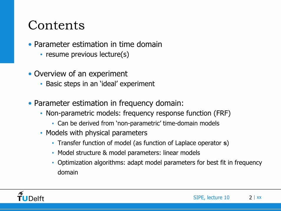
Contents• Parameter estimation in time domain

• resume previous lecture(s)

• Overview of an experiment • Basic steps in an ‘ideal’ experiment

• Parameter estimation in frequency domain:• Non-parametric models: frequency response function (FRF)

• Can be derived from ‘non-parametric’ time-domain models• Models with physical parameters

• Transfer function of model (as function of Laplace operator s)

• Model structure & model parameters: linear models

• Optimization algorithms: adapt model parameters for best fit in frequency

domain


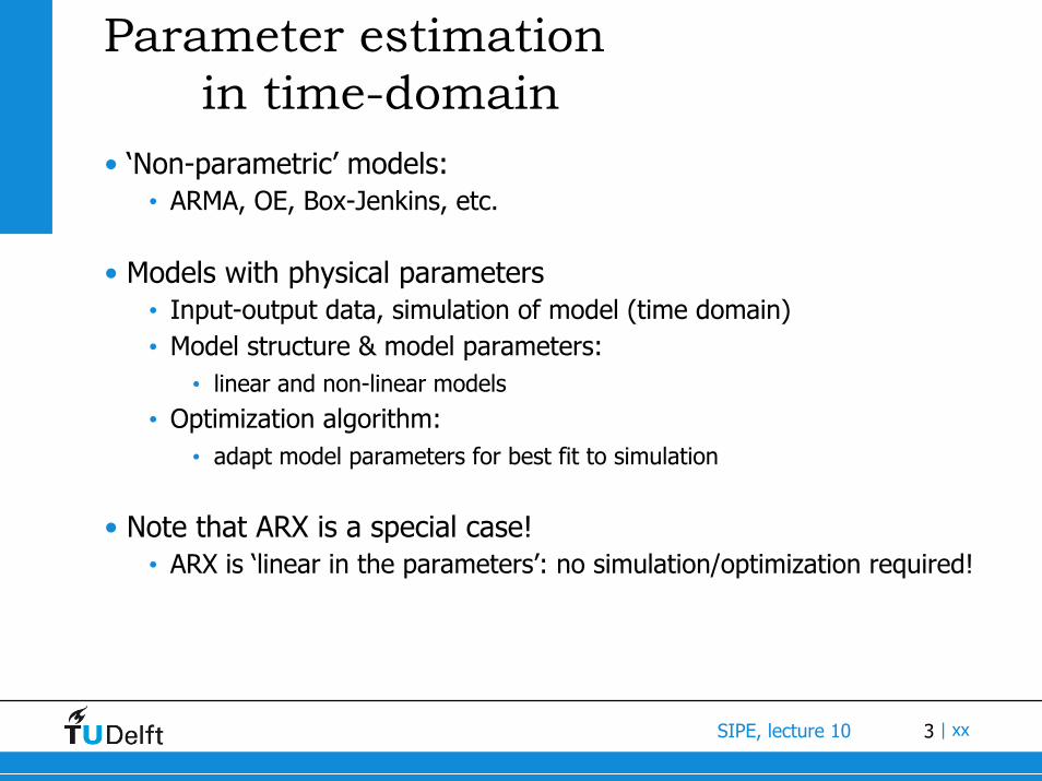
Parameter estimation in time-domain

• ‘Non-parametric’ models:• ARMA, OE, Box-Jenkins, etc.

• Models with physical parameters• Input-output data, simulation of model (time domain) • Model structure & model parameters:

• linear and non-linear models

• Optimization algorithm:• adapt model parameters for best fit to simulation

• Note that ARX is a special case!• ARX is ‘linear in the parameters’: no simulation/optimization required!


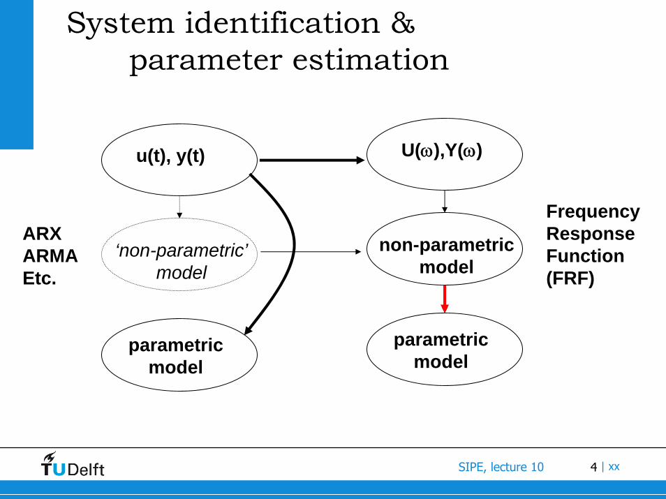
System identification & parameter estimation

u(t), y(t)

‘non-parametric’model

parametricmodel

U(ω),Y(ω)

non-parametricmodel

parametricmodel

ARXARMAEtc.

FrequencyResponseFunction(FRF)


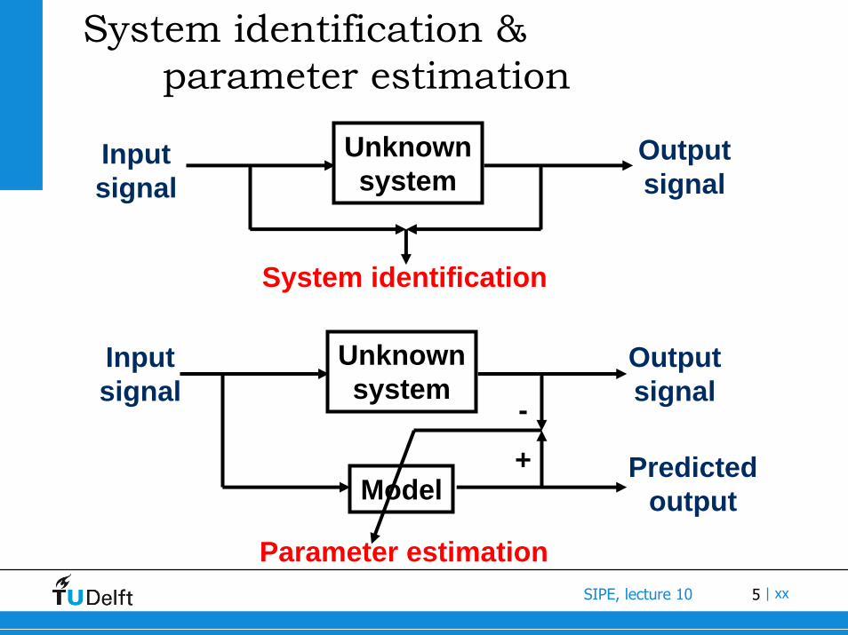
System identification & parameter estimation

Unknownsystem

Inputsignal

Outputsignal

System identification

Unknownsystem

Inputsignal

Outputsignal

ModelPredicted

output+

-

Parameter estimation


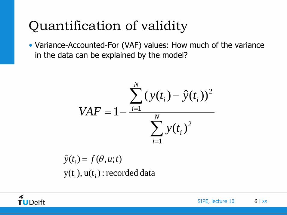
Quantification of validity• Variance-Accounted-For (VAF) values: How much of the variance

in the data can be explained by the model?

∑

∑

=

=

−−= N

ii

N

iii

ty

tytyVAF

1

2

1

2

)(

))(ˆ)((1

data recorded:)u(t ),y(t);,()(ˆ

ii

tufty i θ=


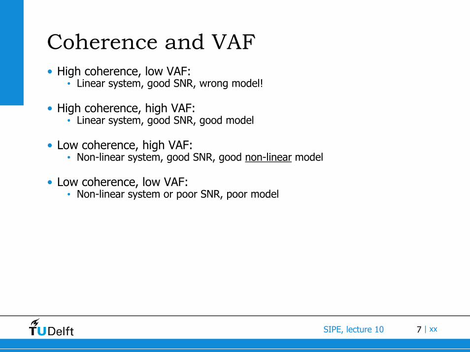
Coherence and VAF• High coherence, low VAF:

• Linear system, good SNR, wrong model!

• High coherence, high VAF:• Linear system, good SNR, good model

• Low coherence, high VAF:• Non-linear system, good SNR, good non-linear model

• Low coherence, low VAF:• Non-linear system or poor SNR, poor model


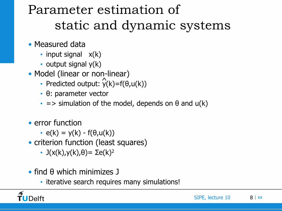
Parameter estimation of static and dynamic systems

• Measured data• input signal x(k)• output signal y(k)

• Model (linear or non-linear)• Predicted output: y(k)=f(θ,u(k))• θ: parameter vector• => simulation of the model, depends on θ and u(k)

• error function• e(k) = y(k) - f(θ,u(k))

• criterion function (least squares)• J(x(k),y(k),θ)= Σe(k)2

• find θ which minimizes J• iterative search requires many simulations!

^


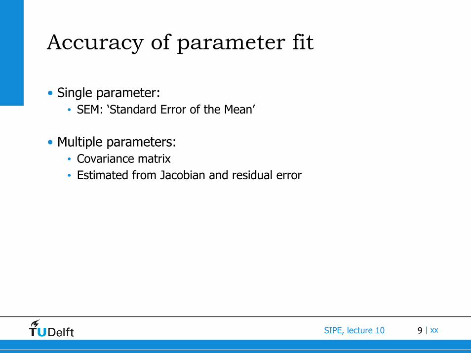
Accuracy of parameter fit

• Single parameter:• SEM: ‘Standard Error of the Mean’

• Multiple parameters:• Covariance matrix• Estimated from Jacobian and residual error


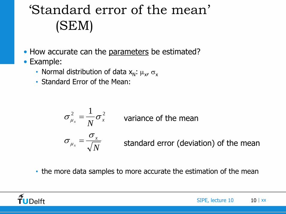
‘Standard error of the mean’(SEM)

• How accurate can the parameters be estimated?• Example:

• Normal distribution of data xN: μx, σx

• Standard Error of the Mean:

• the more data samples to more accurate the estimation of the mean

N

Nx

x

x

x

σσ

σσ

μ

μ

=

= 22 1variance of the mean

standard error (deviation) of the mean


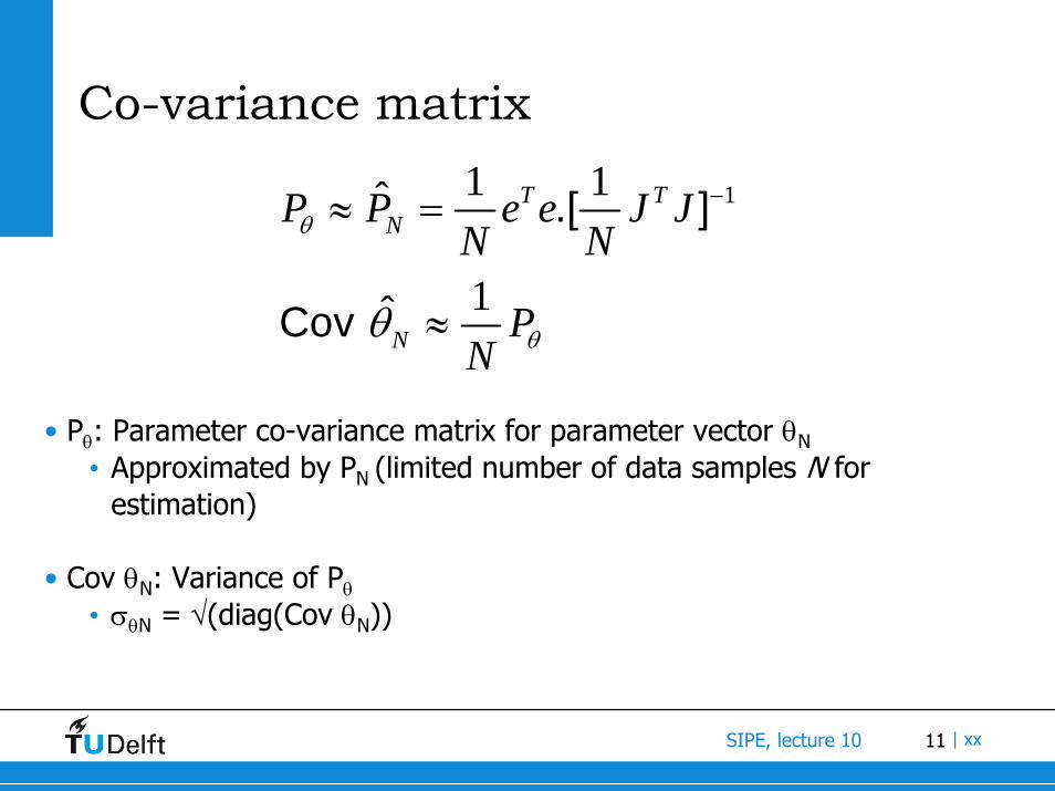
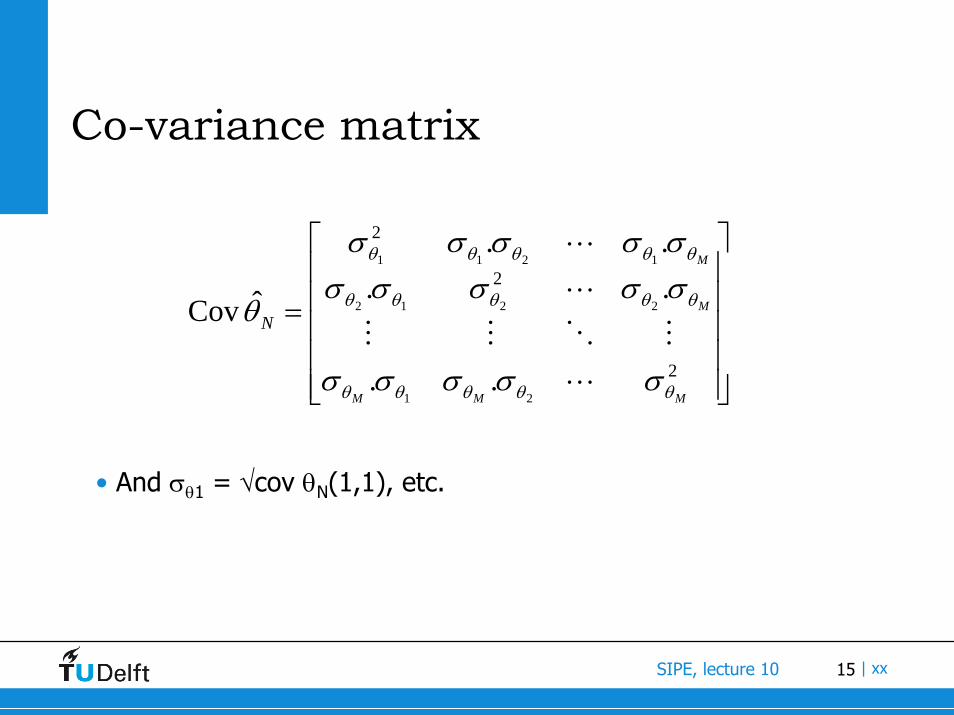
Co-variance matrix

• Pθ: Parameter co-variance matrix for parameter vector θN• Approximated by PN (limited number of data samples N for

estimation)

• Cov θN: Variance of Pθ

• σθN = √(diag(Cov θN))

11 1

1

ˆ .[ ]

ˆCov

T TN

N

P P e e J JN N

PN

θ

θθ

−≈ =

≈


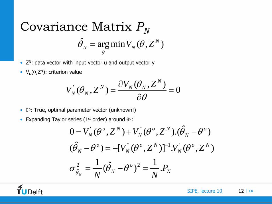
Covariance Matrix PN

• ZN: data vector with input vector u and output vector y

• VN(θ,ZN): criterion value

• θo: True, optimal parameter vector (unknown!)

• Expanding Taylor series (1st order) around θo:

),(minargˆ NNN ZV θθ

θ=

0),(),(' =∂

∂=

θθθ

NNNN

NNZVZV

No

N

NoN

NoN

oN

oN

NoN

NoN

PNN

ZVZV

ZVZV

N.1)ˆ(1

),(.)],([)ˆ(

)ˆ).(,(),(0

22ˆ

'1''

'''

=−=

−=−

−+=−

θθσ

θθθθ

θθθθ

θ


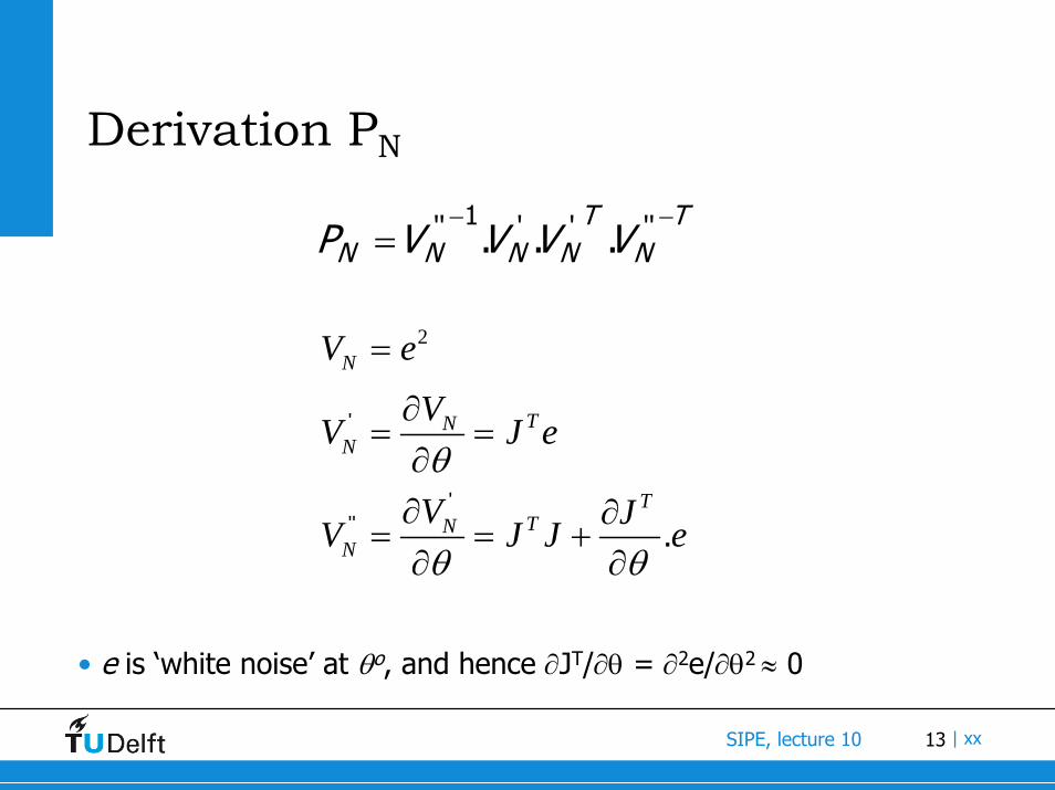
Derivation PN

• e is ‘white noise’ at θo, and hence ∂JT/∂θ = ∂2e/∂θ2 ≈ 0

TN

TNNNN VVVVP

−−= ''''1'' ...

2

'

''' .

N

TNN

TTN

N

V e

VV J e

V JV J J e

θ

θ θ

=

∂= =

∂∂ ∂

= = +∂ ∂


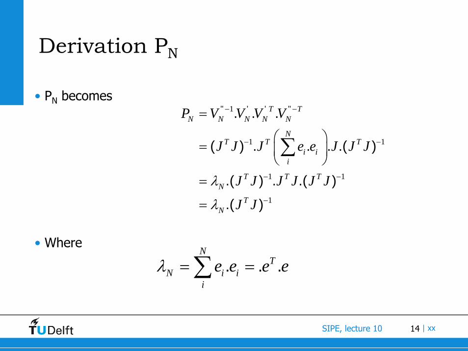
Derivation PN

• PN becomes

• Where

1

1 1

1 1

1

'' ' ' ''. . .

( ) . . . .( )

.( ) . .( )

.( )

T TN N N N N

NT T T

i ii

T T TN

TN

P V V V V

J J J e e J J J

J J J J J J

J J

λ

λ

− −

− −

− −

−

=

⎛ ⎞= ⎜ ⎟

⎝ ⎠=

=

∑

. . .N

TN i i

i

e e e eλ = =∑


Co-variance matrix

• And σθ1 = √cov θN(1,1), etc.

⎥⎥⎥⎥⎥

⎦

⎤

⎢⎢⎢⎢⎢

⎣

⎡

=

2

2

2

21

2212

1211

..

..

..

ˆ Cov

MMM

M

M

N

θθθθθ

θθθθθ

θθθθθ

σσσσσ

σσσσσσσσσσ

θ

L

MOMM

L

L


Matlab demo: parameter accuracy


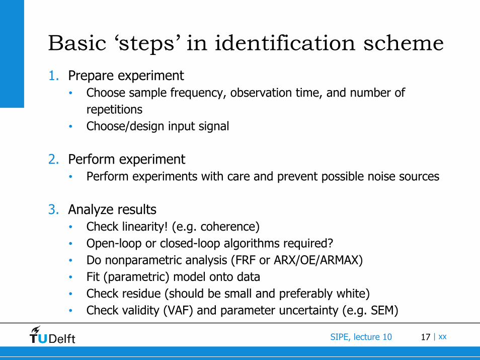
Basic ‘steps’ in identification scheme1. Prepare experiment

• Choose sample frequency, observation time, and number of repetitions

• Choose/design input signal

2. Perform experiment• Perform experiments with care and prevent possible noise sources

3. Analyze results• Check linearity! (e.g. coherence)• Open-loop or closed-loop algorithms required? • Do nonparametric analysis (FRF or ARX/OE/ARMAX)• Fit (parametric) model onto data• Check residue (should be small and preferably white)• Check validity (VAF) and parameter uncertainty (e.g. SEM)


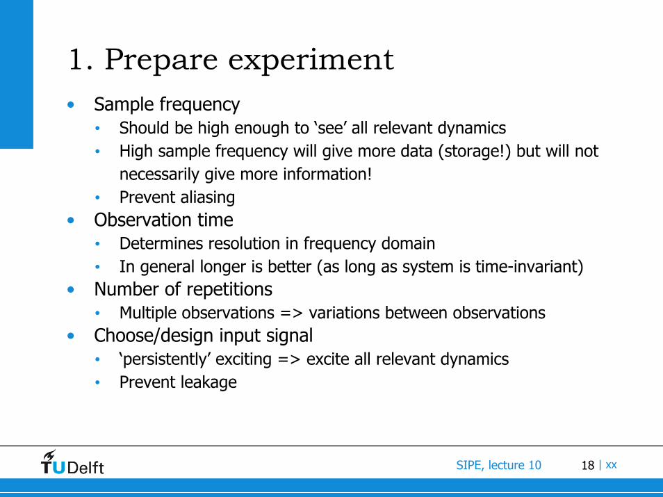
1. Prepare experiment• Sample frequency

• Should be high enough to ‘see’ all relevant dynamics• High sample frequency will give more data (storage!) but will not

necessarily give more information! • Prevent aliasing

• Observation time• Determines resolution in frequency domain• In general longer is better (as long as system is time-invariant)

• Number of repetitions• Multiple observations => variations between observations

• Choose/design input signal• ‘persistently’ exciting => excite all relevant dynamics• Prevent leakage


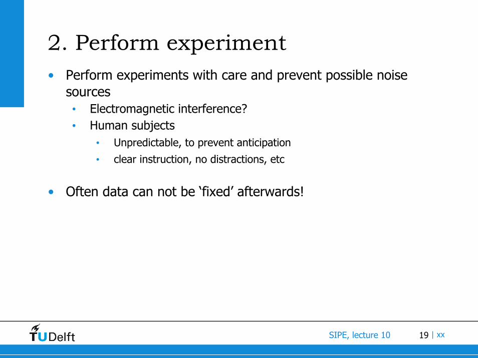
2. Perform experiment• Perform experiments with care and prevent possible noise

sources• Electromagnetic interference?• Human subjects

• Unpredictable, to prevent anticipation

• clear instruction, no distractions, etc

• Often data can not be ‘fixed’ afterwards!


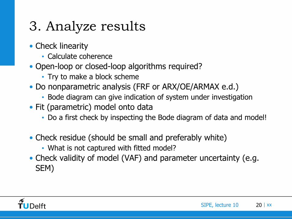
3. Analyze results• Check linearity

• Calculate coherence• Open-loop or closed-loop algorithms required?

• Try to make a block scheme• Do nonparametric analysis (FRF or ARX/OE/ARMAX e.d.)

• Bode diagram can give indication of system under investigation• Fit (parametric) model onto data

• Do a first check by inspecting the Bode diagram of data and model!

• Check residue (should be small and preferably white)• What is not captured with fitted model?

• Check validity of model (VAF) and parameter uncertainty (e.g. SEM)


Options in parameter estimationTime-domain:

• direct fit using derivatives (HMC: inverse dynamics)• Noise is amplified by differentiation

• direct fit using simulation (previous lecture)• Requires multiple model simulations:

a lot of CPU power• Can handle non-linear models!


Options in parameter estimation• Frequency-domain:

1. FFT, estimation of FRF, estimation of parameters• No prior assumptions are needed!• Can easily cope with systems in closed-loop• Estimates can be biased if (very) much noise is present• E.g. depends on number frequency bands used for averaging

2. OE/ARMAX fit, estimation of parameters• In general reasonable fast and accurate• Order selection is needed (requires a choice!)• Frequency reconstruction desired to estimate the model structure (if

system is unknown)


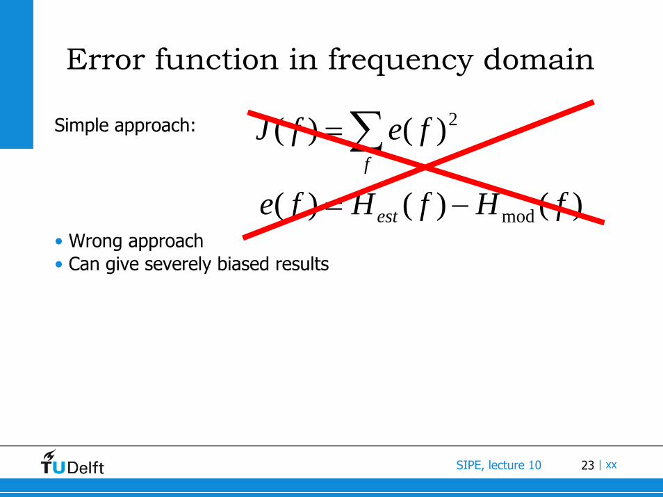
Error function in frequency domain

Simple approach:

• Wrong approach• Can give severely biased results

)()()(

)()(

mod

2

fHfHfe

fefJ

est

f

−=

=∑


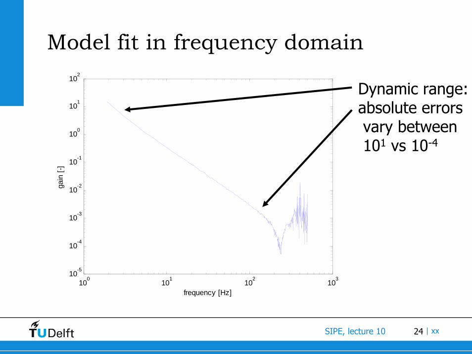
Model fit in frequency domain

100

101

102

103

10-5

10-4

10-3

10-2

10-1

100

101

102

frequency [Hz]

gain

[-]

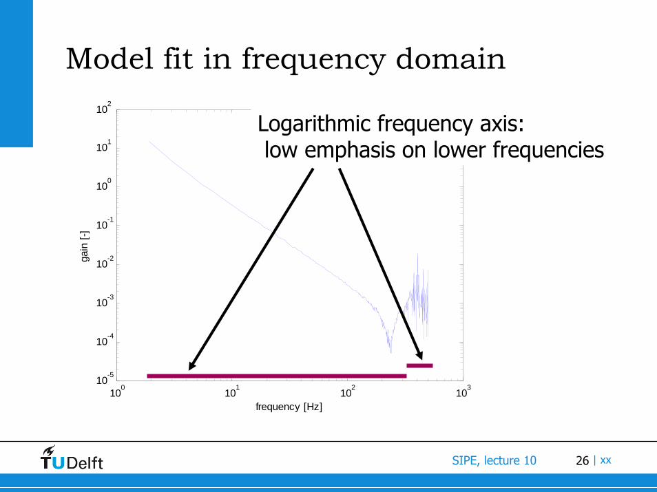
Dynamic range:absolute errors vary between 101 vs 10-4



100 101 102 1030

0.1

0.2

0.3

0.4

0.5

0.6

0.7

0.8

0.9

1

cohe

renc

e [-]

frequency [Hz]

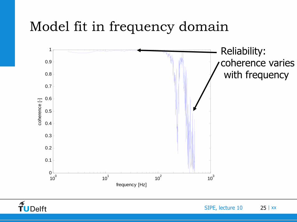
Reliability:coherence varieswith frequency



100

101

102

103

10-5

10-4

10-3

10-2

10-1

100

101

102

frequency [Hz]

gain

[-]

Logarithmic frequency axis:low emphasis on lower frequencies


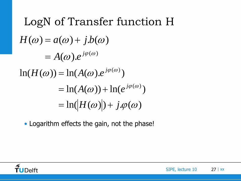
LogN of Transfer function H

)().()(.)()(

ωϕω

ωωωjeA

bjaH=

+=

)(.))(ln()ln())(ln(

)).(ln())(ln()(

)(

ωϕωω

ωωωϕ

ωϕ

jHeA

eAHj

j

+=

+=

=

• Logarithm effects the gain, not the phase!


Error function in frequency domain

regionfrequency lowin data fewfor compensate y to1/frequencby weightedsfrequencie reliableon emphasis moreput tocoherenceby weighted

)()(ln).(.1))(ln())(ln().(.1)(

phase)in difference log(gain)in e(differenc*)(*1 ~

))(())((.()(ln())(ln().(.1

))(ln())(ln().(.1)(

)()(

2

mod

22

mod2

modmod

mod

2

∑∑

∑

⎟⎟⎠

⎞⎜⎜⎝

⎛=−=

+

−+−=

−=

=

f

est

fest

estest

est

f

fHfHf

ffHfHf

ffJ

ff

fHfHifHfHff

fHfHff

fe

fefJ

γγ

γ

ϕϕγ

γ


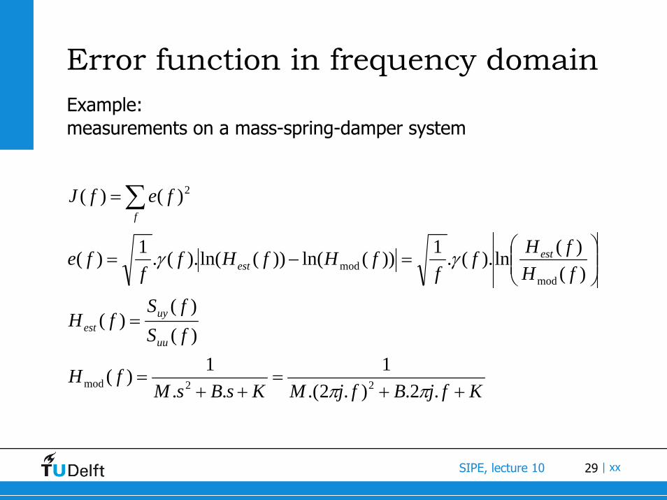
Error function in frequency domainExample:measurements on a mass-spring-damper system

KfjBfjMKsBsMfH

fSfS

fH

fHfHf

ffHfHf

ffe

fefJ

uu

uyest

estest

f

++=

++=

=

⎟⎟⎠

⎞⎜⎜⎝

⎛=−=

=∑

.2.).2.(1

..1)(

)()(

)(

)()(ln).(.1))(ln())(ln().(.1)(

)()(

22mod

modmod

2

ππ

γγ


Assignment this week• Estimate parameters in time and frequency domain• Compare the results between both approaches

• Goal: Show the (dis-)advantages and peculiarities of estimation in both time domain and frequency domain (and compare the two approaches)

system identification parameter estimation - tu delft ocw · system identification & parameter...

Documents