Signal Processing and Communication with Solitons

Andrew C. Singer

RLE Technical Report No. 599

June 1996

The Research Laboratory of ElectronicsMASSACHUSETTS INSTITUTE OF TECHNOLOGY

CAMBRIDGE, MASSACHUSETTS 02139-4307

This research was generously supported in part by the Defense Advanced Research ProjectsAgency under Grant N00014-89-J-1489, in part by Lockheed Martin Sanders, in part by theU.S. Navy Office of the Chief of Naval Research under Grant N00014-93-1-0686, and inpart by U.S. Air Force Office of Scientific Research under Grant AFOSR-91-0034.

Signal Processing and Communication with Solitons

by

Andrew Carl Singer

Submitted to the Department of Electrical Engineering and Computer Scienceon May 14, 1996, in partial fulfillment of the

requirements for the degree ofDoctor of Philosophy

Abstract

Traditional signal processing algorithms rely heavily on models that are inherentlylinear. Such models are attractive both for their mathematical tractability and theirapplicability to the rich class of signals that can be represented with Fourier methods.Nonlinear systems that support soliton solutions share many of the properties thatmake linear systems attractive from an engineering standpoint. Although nonlinear,these systems are solvable through inverse scattering, a technique analogous to theFourier transform for linear systems. Solitons are eigenfunctions of these systemswhich satisfy a nonlinear form of superposition and display rich signal dynamics asthey interact. By using solitons for signal synthesis, the corresponding nonlinearsystems become specialized signal processors which are naturally suited to a numberof complex signal processing tasks. Specific analog circuits can generate soliton signalsand can be used as natural multiplexers and demultiplexers in a number of potentialsoliton-based wireless communication applications. These circuits play an importantrole in investigating the effects of noise on soliton behavior. Finally, the soliton signaldynamics also provide a mechanism for decreasing transmitted signal energy whileenhancing signal detection and parameter estimation performance.

Thesis Supervisor: Alan V. OppenheimTitle: Distinguished Professor of Electrical Engineering and Computer Science

Acknowledgments

I would like to express my sincere gratitude to Professor Alan Oppenheim, for bothputting me out on a limb, and for making sure that I did not fall. Through his manyroles as an advisor, a mentor, and above all, as a friend, he has had a tremendousimpact on both my professional and personal development. I look forward to exploringmany more trees together.

For his guidance, encouragement, and friendship, I also wish to thank ProfessorGregory Wornell. Our many discussions have greatly influenced the way I think aboutresearch problems in general and this thesis in particular. I am sincerely gratefulto Professor Ruben Rosales for his many insightful comments, his interest and hisencouragement. Thanks also to Dr. Jim Kaiser of Bellcore and Dr. Doug Mook ofLockheed Sanders for numerous discussions relating to this work. Lloyd D'Souzadeserves thanks for his many hours of circuit hacking and development.

The friendly atmosphere and productive research environment of the Digital SignalProcessing Group have made my experiences as a graduate student both challengingand rewarding. Thanks to John Buck, Babis Papadopoulos, and Kathleen Wage fortheir help with various parts of this thesis and to Paul Beckmann, Steve Isabelle,Stephen Scherock, and Kambiz Zangi for many years of friendship and thought-provoking discussion. Thanks also to Jeff Ludwig, Lon Sunshine and Yakov Royterfor their camaraderie and our many athletic pursuits.

I am especially grateful to Giovanni Aliberti both for his computer expertise andfriendship. Special thanks go to Maggie Beucler, Janice Zaganjori and Sally Bemusfor administrative support and for help in preparing this document.

This research has been generously supported by the Defense Advanced ResearchProjects Agency, Lockheed Martin Sanders, the Department of the Navy Office ofthe Chief of Naval Research, and the Air Force Office of Scientific Research.

Finally, I would like to thank my parents for their love and support and for beingmy very first teachers. Also, thanks to my sister Amy for reminding me what it'slike to be a big brother. Most importantly, thanks to my loving wife, Cathy, for herunending love and encouragement.

Contents

1 Introduction1.1 Outline of the Thesis .............

2 Soliton Systems2.1 The Toda Lattice ...............2.2 The Inverse Scattering Transform ......2.3 Other Systems Exhibiting Solitons .....2.4 Soliton Hierarchies .............2.A A Soliton Solution ..............2.B Multi-soliton Solutions ...........2.C Single Pole Reflection Coefficient ......

3 New Electrical Analogs for Soliton Systems3.1 Toda Circuit Model of Hirota and Suzuki . .3.2 Diode Ladder Circuit Model for Toda Lattice3.3 Circuit Simulation3.4 Circuit Implementation ....3.5 Circuit Model for Discrete-KdV3.6 Further Considerations ....

4 Communication with Soliton Signals4.1 Soliton Modulation ..............4.2 Soliton Multiplexing .............4.3 Spectrum of Toda Lattice Solitons ......4.4 Low Energy Signaling. ............4.5 Gain Normalization .............4.6 Other Potential Applications .........

5 Noise Dynamics in Soliton Systems5.1 Toda Lattice Small Signal Model ......5.2 Linearized Model ...............5.3 Simulation of the Lattice in Noise ......5.4 Noise Correlation ...............5.5 Noise Dynamics for the Diode Ladder Circuit5.6 Inverse Scattering-Based Noise Modeling ....

5

11. . .. . . . . . . 12

1516222830343536

39. . . .. . . . . . . 41. . . .. . . . . . . 43. . . .. . . . . . . 45. . . .. . . . . . . 48. . . .. . . . . . . 52. . . .. . . . . . . 57

61626366697477

81. . . .. . . . . . . . . . 83. . . .. . . . . . . . . . 85. . . .. . . . . . . . . . 87. . . .. . . . . . . . . . 89

. . . .. . . . . . . . . 9597

..............

..............

..............

..............

..............

..............

..............

.................. . . . . . . . . .

· .

..............

..............

..............

..............

..............

..............

6 Estimation of Soliton Signals6.1 Soliton Parameter Estimation: Bounds .....6.2 Multi-soliton Parameter Estimation: Bounds6.3 Estimation Algorithms .............

6.3.1 General Approach ............6.3.2 Position Estimation ...........6.3.3 Velocity Estimation ...........6.3.4 Estimation Based on Inverse Scattering .

6.4 Summary .....................

103..... 104..... 107..... 110..... 110..... 114..... 115..... 116..... 120

7 Detection of Soliton Signals7.1 General Approach ................7.2 Simulations ....................7.3 Summary and Further Considerations ......

8 Conclusions and Directions for Future Work8.1 Future Directions ................

123123127128

131133

6

List of Figures

2-1 The Toda Lattice .......................................... 162-2 A propagating wave solution to the Toda lattice equations. Each trace

corresponds to the force f (t) stored in the spring between mass n andn-1 . ....................... . . . . . . . . . . . . 17

2-3 Two solitary wave solutions to the Toda lattice ................. . 202-4 Spectrum of eigenvalues of the matrix L(t) for the Toda lattice. ... . 242-5 Schematic solution to linear evolution equations ............. 252-6 Schematic solution to soliton equations .................. 252-7 Soliton-like solutions to the automata of Ablowitz et al ......... 31

3-1 Two-soliton signal processing by a soliton system ............ 403-2 Nonlinear LC ladder circuit of Hirota and Suzuki ............ 413-3 Diode ladder network ..................................... . 433-4 Double capacitor circuit diagram ..................... 443-5 HSPICE simulation of the evolution of a two-soliton signal through the

diode lattice. Each horizontal trace shows the current through one ofthe diodes 1, 3,4 and 5 . . . . . . . . . . . . . . . . . . . . . . . . . 47

3-6 Precision bipolar current source ...................... 493-7 Diagram for the double capacitors used in the diode ladder circuit.

Analog switches, placed in parallel with the capacitors, are used toreset the circuit after each processed signal ............... 50

3-8 Hardware implementation of the diode ladder circuit. The first col-umn from the left contains the pulse-generation circuitry; the secondcontains the voltage-controlled current source; each of the last threecontains four stages of diodes, series resistors and double capacitors.. 51

3-9 Oscilloscope traces for two solitons in the diode ladder circuit. Thetraces correspond to the currents in the first four diodes ....... . 52

3-10 Diode currents measured from the diode ladder circuit in operation.The input signal consists of three square pulses of different areas. Thespike that appears in the figure near t = -1 ms is a result of the signalthat resets the lattice ..................................... . 53

3-11 Illustration of the relationship between two adjacent Toda lattices,fi,, i = 1,2 and the discrete-KdV equation. This process suggestsa possible implementation of the dKdV equation using two adjacentToda lattice circuits ............................ 55

3-12 Collection of nodes for the discrete-KdV circuit ............. 56

7

3-13 To the left, the normalized node capacitor voltages, vn(t)/vt for eachnode is shown as a function of time. To the right, the state of the circuitis shown as a function of node index for five different sample times. Thebottom trace in the figure corresponds to the initial condition .. . 58

4-1 A soliton carrier signal for the Toda lattice ............... 624-2 Modulating the relative amplitude or position of soliton carrier signal

for the Toda lattice ............................. 634-3 Multiplexing of a four soliton solution to the Toda lattice ...... . 644-4 Toda lattice response to an outgoing signal at node 0 and to a received

signal at node 35, each with three component solitons. The solitonsthat are input at node 0 are multiplexed by the system, as viewed onnode 35. The solitons that are input to node 35, propagate in thereverse direction, and are demultiplexed by the system, as viewed onnode 0 . . . . . . . . . . . . . . . . . . . . . . . . . . . . . . . . . . 65

4-5 A two-soliton solution is depicted in the Toda lattice. Each horizontaltrace is the response at a successive node in the lattice. In this case,the two soliton wavenumbers are Pi = 2 and P2 = 1.3 .......... 71

4-6 A two-soliton solution to the Toda lattice as a function of both timeand mutual separation, 61 - 2 ...................... 74

4-7 Normalized signal energy for a two-soliton solution to the Toda latticeholding 1 fixed for 3 values of 2. The signal energy is normalized bythe maximum signal energy of the separated solitons ............ . 75

4-8 Normalized cross-covariance of input with the processed signal as afunction of the unknown gain, ca ..................... 76

4-9 Schematic diagram of AM-like modulation of Hirota and Suzuki. Re-drawn based on [64, 65] ............ ......................... 79

5-1 The log magnitude of the frequency response from the input node tothe N-th node as a function of normalized frequency. As indicated,the response rapidly drops off as a function of N for w > wc .. ... 86

5-2 Receiver model comprising a low pass filter followed by a Toda latticecircuit ............................................... 87

5-3 Response to a single soliton with = sinh(1) in 20 dB Gaussian noise.The spectrum of the noise process is flat out to half the sample-rateof the integration routine. The corresponding in-band SNR is approx-imately 24 dB ............................... 89

5-4 Noise response to a single soliton in 20 dB Gaussian noise as viewedfrom the third node in the lattice ..................... 90

5-5 Response to a single soliton with /3 = sinh(1) in 10 dB Gaussian noise. 915-6 Cross-correlation, Rm,n(T), between the m-th and the n-th node volt-

ages in the linearized lattice ................................. 925-7 The variance of each node voltage as a function of time ......... 94

8

6-1 The Cramdr-Rao lower bound for estimating 1 = sinh(2) and 2 =

sinh(1.75) with all parameters unknown in AWGN with No = 1. Thebounds are shown as a function of the relative separation, 6 = 61 - 2.

The CRB for estimating 1 and 2 of a single soliton with the sameparameter value is indicated with 'o' and 'x' marks, respectively. . . 109

6-2 The Cramdr-Rao lower bound for estimating 1 = sinh(2) and /2 =

sinh(1.25) with all parameters unknown in AWGN with No = 1. Thebounds are shown as a function of the relative separation, 6 = 61 - 2.

The CRB for estimating /31 and 2 of a single soliton with the sameparameter value is indicated with 'o' and 'x' marks, respectively. . . 110

6-3 The Cramdr-Rao bounds for estimating the time of arrival for eachsoliton in a two-soliton signal with /1 = sinh(2) and 32 = sinh(1.25)in AWGN with No = 1. The asymptotic values of each of the boundsagree with the CRB for estimating the time of arrival of a single solitonwith the same parameter value as indicated with 'o' and 'x' marks. . 111

6-4 Toda lattice receiver model . . . . . . . . . . . . . . . . . . . . . . . 1146-5 The CRBs for 61 and 2 are shown with solid and dashed lines, while

the estimation error results of 100 Monte-Carlo trials are indicatedwith 'o' and 'x' marks, respectively ...................... 115

6-6 The estimation error variance for the velocity-based algorithm. TheCRB for /1 and 2 is shown with a solid and dashed line, and theestimation error variances are indicated by the points labeled 'o' and' x' respectively . . . . . . . . . . . . . . . . . . . . . . . . . . . . . . 117

6-7 Procedure for computing L(t) by processing the signal r(t) with theToda lattice . . . . . . . . . . . . . . . . . . . . . . . . . . . . . . . 118

6-8 The estimation error variance for the inverse scattering-based estimatesof 1 = sinh(2), 2 = sinh(1.5). The bounds for 1 and 2 are indicatedwith solid and dashed lines respectively. The estimation results for 100Monte Carlo trials with a diode lattice of N = 10 nodes for /31 and 2

are indicated by the points labeled 'o' and 'x' respectively ....... 1206-9 Normalized mean parameter estimation error for the inverse scattering-

based estimation . . . . . . . . . . . . . . . . . . . . . . . . . . . . . 1216-10 The estimation error variance for estimating 1 = sinh(2), 2 = sinh(1.5)

are indicated with the points labeled 'o' and 'x' and the CRBs for eachare indicated with solid and dashed lines, respectively .......... 122

7-1 A set of empirically generated ROCs are shown for the detection ofthe smaller soliton from a two-soliton signal. For each of the threenoise levels, the ROC for detection of the smaller soliton alone is alsoindicated along with the corresponding detection index, d ...... . 128

9

10

Chapter 1

Introduction

Many traditional signal processing applications rely on models that are inherently lin-

ear and time-invariant (LTI). Much of the success of such methods can be attributed

to their being mathematically tractable, often leading to efficient signal representa-

tions and fast algorithms. Linear techniques have also proven effective for modeling

a variety of signals of practical interest such as speech or financial time-series and

systems of interest such as the telephone or radio broadcast channels. However, we

increasingly turn to nonlinear models to capture some of the more salient behavior of

physical or natural systems that cannot be expressed by linear means, such as thresh-

old phenomena, amplitude-dependence, or chaotic behavior. Nonlinear systems also

hold the potential to produce more efficient algorithms or models for a variety of signal

processing and communication problems where linear techniques are suboptimal.

Systems that support solitons may be a natural choice for a class of nonlinear

systems to explore since they share many of the properties that make LTI systems

attractive from an engineering standpoint. Although nonlinear, these systems are

solvable through inverse scattering, a technique analogous to the Fourier transform

for linear systems [1]. Solitons are eigenfunctions of these systems which satisfy a non-

linear form of superposition. We can therefore decompose complex solutions in terms

of a class of signals with simple dynamical structure. Solitons have been observed in a

variety of natural phenomena from water and plasma waves [31, 57] to crystal lattice

vibrations [14] and energy transport in proteins [31]. Solitons can also be found in

11

a number of man-made media including super-conducting transmission lines [56] and

nonlinear circuits [29, 60]. Recently, solitons have become of significant interest for

optical telecommunications, where optical pulses have been shown to propagate as

solitons for tremendous distances without significant loss or dispersion [23].

In this thesis, we view solitons from a decidedly different perspective. Rather than

focusing on the propagation of solitons over nonlinear channels, we consider using

these nonlinear systems to both generate and process signals for transmission over

traditional linear channels. By using solitons for signal synthesis, the corresponding

nonlinear systems become specialized signal processors which are naturally suited

to a number of complex signal processing tasks. This thesis can be viewed as an

exploration of the properties of solitons as signals. In the process, we explore the

possibility of using these signals in a potential multi-user wireless communication

context.

For example, we consider the problem of multiplexing a number of users onto a

single carrier for transmission over a lossy channel. A variety of linear multiplexing

schemes have been proposed such as time-, frequency-, or code-division multiple access

systems. However, the number of nonlinear multiplexing strategies available is rather

limited. One potential benefit to using solitons as carrier signals and the nonlinear

systems as multiplexors, is that the soliton signal dynamics provide a mechanism for

simultaneously decreasing transmitted signal energy and enhancing communication

performance.

1.1 Outline of the Thesis

There is a large body of literature on soliton theory spanning over a century of re-

search. Rather than attempting to provide a self-contained summary, in Chapter 2

we present a brief overview of the components of soliton theory that we will draw

upon throughout the thesis. The chapter includes an introduction to solitons and

some of the nonlinear systems that support them. We focus our discussion on the

Toda lattice, a particularly simple soliton system that forms the basis of many of our

12

examples throughout the thesis. In order to exploit the rich mathematical structure

of these systems, we review some elements from inverse scattering theory. In addi-

tion to providing an efficient mechanism for the construction of soliton signals and

the solutions to their dynamics, the inverse scattering framework can also be used

to synthesize families of soliton systems. Throughout the thesis, the inverse scatter-

ing transform plays an analogous role to the Fourier transform in the analysis and

processing of soliton signals in the presence of noise.

To facilitate real-time generation and processing of soliton signals, it will be im-

portant to explore implementations of these nonlinear systems. In Chapter 3 we

develop new circuit models for two soliton systems. The first is a diode ladder imple-

mentation of the Toda lattice which appears to be the first circuit implementation to

display true soliton behavior. We also develop a lattice-circuit implementation of the

discrete-KdV equation, which will be important for processing discrete-time soliton

signals.

These circuit models then form the basis for a communication paradigm presented

in Chapter 4, where multiple signals can be multiplexed onto soliton carriers using

such circuits as tuned modulators and demodulators. As we will see, the nonlinear in-

teraction of multiple solitons can be exploited as a means for reducing the transmitted

signal energy in a multi-user communication context. Such low power transmission

techniques may be applicable to a variety of portable or power-limited communication

applications.

Before soliton systems can be used in a practical communication context, we need

accurate models for the effects of disturbances on the dynamics of these systems. The

robustness of such systems to additive corruption will have a direct impact on the

demodulation performance of the nonlinear receivers. In Chapter 5, we analyze the

effects of small amplitude corruption on the dynamics of solitons in the Toda lattice

and characterize the statistics of the noise as it is propagates through the system.

In order to develop effective communication strategies by modulating the param-

eters of soliton carriers, we need to have accurate models for the ability of a receiver

to resolve these parameters. In Chapter 6, we compute Cramer-Rao bounds for their

13

estimation error variance. We show that in addition to reducing signal energy, the

nonlinear interaction of multiple solitons can also enhance parameter estimation per-

formance. Based on our characterization of the noise, we develop a set of parameter

estimation algorithms in which maximum-likelihood (ML) estimates can be obtained

from corrupted measurements. In Chapter 7, we demonstrate how soliton circuits can

be used to enhance the detection of multiple solitons in noise.

Finally, Chapter 8 summarizes the main contributions of the thesis and indicates

some interesting and potentially important directions for future study.

14

Chapter 2

Soliton Systems

Solitons play an important role in the study of a large class of nonlinear evolution

equations. As we shall see, the ability to describe their long-term behavior analytically

makes this class of systems attractive for modeling a variety of nonlinear phenomena

in a number of diverse areas in mathematics, physics, biology, and engineering. Ex-

amples include topics from surface or internal water waves, to energy transport along

long protein chains, and the propagation of optical pulses along nonlinear fibers. Fur-

thermore, the development of optical and electrical analogs for many of these systems

makes soliton signals of great practical interest.

The theory of solitons dates back to the work of Korteweg and de-Vries, and

was motivated by attempts to explain the unusual water wave observations of Scott

Russell in 1834. The method of solution for soliton systems began with the work of

Gardner, Greene, Kruskal, and Miura on the Korteweg-de Vries (KdV) equation [18].

These techniques were generalized by Lax [42] and then by Ablowitz et al. [1] and

used to solve what is now a large class of solvable nonlinear evolution equations.

This chapter is designed as a brief overview of the components of soliton theory

that we will draw upon throughout the thesis. Although no new results will be

presented, this chapter serves several purposes. First, we present an introduction to

solitons and to some of the nonlinear systems that support them. We will focus our

attention on the Toda lattice, a simple mechanical system that will form the basis

of many of the examples throughout the thesis. Second, we summarize some of the

15

Yn- 1 Yn Yn+

Figure 2-1: The Toda Lattice.

main results of inverse scattering theory, the method by which soliton systems can be

solved analytically. Rather than attempting to fully develop this topic, we concentrate

on portions of the theory that we will exploit in the applications developed in later

chapters of the thesis. Finally, we mention a few of the techniques that can be used to

construct families of soliton systems. As we will see in later chapters, these systems

are potentially useful for a number of communication applications. Therefore, there

may be a practical use for the generation of increasingly complex soliton systems.

2.1 The Toda Lattice

The Toda lattice is a conceptually simple mechanical example of a nonlinear system

with soliton solutions. A comprehensive treatment of the lattice and its associated

soliton theory can be found in the monograph by Toda [69]. As shown in Fig. 2-1,

the Toda lattice equations describe the displacements of an infinite chain of masses

connected with nonlinear springs. Each of the springs satisfies the nonlinear force law

f = a(e - b(Yn- y n- ) - 1), (2.1)

where fn is the force on the spring between masses with displacements Yn and Yn-1

from their rest positions. The equations of motion for the lattice are given by

mnn = a (e - b (y . -y r - l) -e-b(y,+l-Yn)) (2.2)

16

35-

30

X 250

.: 20C,)(/)

15E

10 I

5

5 10 15 20 25 30time

Figure 2-2: A propagating wave solution to the Toda lattice equations. Each tracecorresponds to the force f(t) stored in the spring between mass n and n - 1.

where y, is the displacement of the n-th mass from its rest position, m is the mass,

and a and b are constants. This equation admits pulse-like solutions of the form

f (t) = (m) b 2sech2(sinh(m /ab 3)n- t), (2.3)

which propagate as compressional waves stored as forces in the nonlinear springs. A

single right-traveling wave f(t) is shown in Fig. 2-2. The bottom trace in the figure

corresponds to the force in the spring between masses "zero" and "one" of an infinite-

length Toda chain. This compressional wave is localized in time, and propagates along

the chain maintaining constant shape and velocity. Since, for example, the wave

fn(t) appears on the thirtieth mass at a later point in time, this wave is therefore

propagating to the right along the lattice as viewed in Fig. 2-1. The parameter /3

appears in both the amplitude and in the temporal- and spatial-scales of this one-

parameter family of solutions giving rise to tall, narrow pulses which propagate faster

then small, wide pulses. This type of localized pulse-like solution is what is often

referred to as a solitary wave.

17

Definition 1: A solitary wave solution to a partial differential equation for de-

pendent variable, y, with temporal and spatial variables, t and n, is a traveling-wave

solution of the form,

y(n, t) = f (n - ct) = f (z), (2.4)

where c is a fixed constant, and the energy of f (z) is localized.

The history of solitary waves dates back to the work of John Scott Russell in 1834

and perhaps the first recorded sighting of a solitary wave. Here is his original account

of his sighting:

I was observing the motion of a boat which was rapidly drawn alonga narrow channel by a pair of horses, when the boat suddenly stopped-not so the mass of water in the channel which it had put in motion; it ac-cumulated round the prow of the vessel in a state of violent agitation, thensuddenly leaving it behind, rolled forward with great velocity, assumingthe form of a large solitary elevation, a rounded, smooth and well definedheap of water, which continued its course along the channel apparentlywithout change of form or diminution of speed. I followed it on horsebackand overtook it still rolling on at a rate of speed some eight or nine milesan hour, preserving its original figure some thirty feet long and a foot toa foot and a half in height. Its height gradually diminished and after achase of one or two miles I lost it in the windings of the channel. Such inthe month of August 1834 was my first encounter with that singular andbeautiful phenomenon... [58].

What Scott Russell actually observed was a solitary wave solution to what is

now known as the KdV equation [57]. The Toda lattice is in many ways analogous

to KdV; in fact, KdV can be derived as a continuum limit. A detailed discussion of

linear and nonlinear wave theory including KdV can be found in [75]. In a 1965 paper,

Zabusky and Kruskal performed numerical experiments with KdV and noticed that

these solitary wave solutions retained their identity upon collision with other solitary

waves. Since the velocities of KdV solitary waves are proportional to their amplitudes,

a collision of solitary waves will occur for any solution with a taller pulse to the left of

a shorter pulse. As the individual solitary waves approach one-another, they begin to

interact nonlinearly. However, after passing through one-another, they regain their

shape and speed with only a slight positional shift as evidence of their interaction [78].

18

This process indicates that the nonlinear dynamic system has a generalized coordinate

transformation, or underlying dynamic structure which produces a set of "normal

modes" that are almost completely uncoupled.

Zabusky and Kruskal's discovery that these solitary wave solutions behaved much

like particles in that they essentially retained their identity after collisions prompted

them to coin the term soliton implying that these solitary waves possess a particle-

like nature. This is the type of behavior we would expect for linear wave equations,

that is, the ability to form solutions from a superposition of simpler waves. However,

that a nonlinear equation such as KdV or the Toda lattice permits such a form of

superposition is an indication that it belongs to a rather remarkable class of nonlinear

systems. This property distinguishes solitons from other solitary waves. We will adopt

the following working definition of solitons:

Definition 2: A soliton solution to a partial differential equation is a solitary wave

which asymptotically retains its shape and velocity upon collision with another soliton,

i.e.

y(n,t) = { f (n - ct), t -oo, (2.5)f (n - ct + ), t +oo,

for (n - ct) fixed and 6 an arbitrary constant.

As we shall see, the term soliton often implies additional mathematical structure

involving the inverse scattering transform.

Returning to the Toda lattice, Fig. 2-3 illustrates soliton behavior for two solutions

of the form of Eq. (2.3). The bottom trace in the figure corresponds to the force in the

spring between masses with indices zero and one in the lattice. Note that as a function

of time, a smaller, wider soliton appears before a taller, narrower one. However, as

viewed by, e.g., the thirtieth mass in the lattice, the larger soliton appears first as a

function of time, i.e. has traveled faster. Note that when the larger soliton catches up

to the smaller soliton as viewed on the fifteenth node, the combined amplitude of the

two solitons is actually less than would be expected for a linear system, which would

display a linear superposition of the two amplitudes. Also, the signal shape changes

19

timeFigure 2-3: Two solitary wave solutions to the Toda lattice.

significantly during this nonlinear interaction. Both of these characteristics of soliton

interaction will have useful implications in the context developed in Chap. 4.

An analytic expression for the two-soliton solution for 1 > 2 > 0 is given by [29]

m /32sech2 (l7) + 2sech2 (r 2) + Asech2 ( /71)sech 2 (72) (26)fn(t) ab (cosh(q/2) + sinh(0/2) tanh(71l) tanh(712)) 2 (2.6)

where

A = sinh(0/2) ((3,2 +322) sinh(q/2) + 2132 cosh(q/2)), (2.7)

and

= n (sinh((pi + P2)) ' (2.8)

and i = ab/msinh(pi), and qi = pin - i(t - i).

Although Eq. (2.6) appears rather complex, Figure 2-3 illustrates that for large

separations, J5 - 21, f(t) essentially reduces to the linear superposition of two

solitons with parameters 31 and 2. As the relative separation decreases, the multi-

plicative cross term becomes significant, and the solitons interact nonlinearly. This

20

lo0

asymptotic behavior can also be evidenced analytically,

fn (t) = bp1sech2(pn - Pl(t - 1) ± b/2)

+ b2sech2(p2n-2(t-2) /2), t o,+ -3 2sech (P2 n - 0( - 2) T: q$/2), t -+ +oo,ab

(2.9)

where each component soliton experiences a net displacement X from the nonlinear

interaction.

The Toda lattice also admits periodic solutions which can be written in terms of

Jacobian elliptic functions dn(.) and sn(-). These solutions can be expressed

(2Kv) 2f (t) = ab/m {dn2 [2 (n ±vt)] } E

for wavelength A and frequency v, with

-1/22Kv = a (sn- 2 (2K/A) -

For further description of Jacobian elliptic functions, the reader is referred to [2]

and [69].

An interesting observation can be made when the Toda lattice equations are writ-

ten in terms of the forces,

dt/2 fn dt2 a 1 bm f+ - 2fn + fA-l).

If the substitutionfd 2(t) n (t)fn (t) =--t- In Obn(t) (2.13)

is made into Eq. (2.12), then the lattice equations become,

(2_- .) = t2- _,+ab n-O& n1nl (2.14)

In view of the Teager energy operator introduced by Kaiser in [35], the left hand side

of Eq. (2.14) is the Teager instantaneous-time energy at the node n, and the right

21

(2.10)

(2.11)

(2.12)

hand side is the Teager instantaneous-space energy at time t. In this form, we may

view solutions to Eq. (2.14) as propagating waveforms that have equal Teager energy

as calculated in time and in space, a relationship also observed by Kaiser [36].

2.2 The Inverse Scattering Transform

Perhaps the most significant discovery in soliton theory was that under a rather gen-

eral set of conditions, certain nonlinear evolution equations such as KdV or the Toda

lattice could be solved analytically. That is, given an initial condition of the system,

the solution can be explicitly determined for all time. This discovery eventually led to

a theory of solvable nonlinear dynamic systems to which KdV and Toda belong along

with many other nonlinear systems which exhibit soliton behavior. Since much of

inverse scattering theory is beyond the scope of this thesis, we will only present some

of the basic elements of the theory which we will exploit in later chapters and refer

the interested reader to the comprehensive treatment given in the text by Ablowitz

and Clarkson [1].

The nonlinear systems which have been solved by inverse scattering belong to a

class of systems called conservative Hamiltonian systems. These are state-variable

systems where the dynamics can be written explicitly in terms of the gradient of an

energy function, or the Hamiltonian of the system, '7(x). For example, if the state

of the system were given by x, and the Hamiltonian were 7/(x), then the dynamics

could be written in the form

[ I V]/(x). (2.15)-I 0

For conservative Hamiltonian systems, )i(x) will not be a function of time. A rigorous

treatment of Hamiltonian systems can be found in the text [41]. Conditions under

which conservative Hamiltonian systems become solvable can be found in [3]. For the

nonlinear systems we discuss in this thesis, an integral component of their solution lies

in the ability to write the dynamics of the system implicitly in terms of an operator

22

differential equation of the form,

dL(t) = B(t) L (t) - L(t) B (t), (2.16)dt

where L(t) is a symmetric linear operator, B(t) is an anti-symmetric linear operator,

and both L(t) and B(t) depend explicitly on the state of the system x(t). Lax has

shown [42] that when the dynamics can be written in the form of Eq. (2.16), then

the eigenvalues of the operator L(t) are time-invariant, i.e. = 0. The ability to

write the dynamics implicitly in the form of Eq. (2.16), coupled with the structure of

conservative Hamiltonian systems is sufficient to guarantee the solvability of each of

the soliton systems that will be discussed in this thesis.

Using the Toda lattice as an example, the operator L would be the symmetric

matrixanl-1

L= an-1 bn an , (2.17)

an °o

where

a = e( nyn+2 b (2.18)2 2'

for mass positions yn in a solution to Eq. (2.2). When B is given by the anti-symmetric

matrix

-an-1

B = an- 1 0 -an , (2.19)

an

then Eq. (2.16) implicitly contains the Toda lattice equations. Although each of the

entries of L(t) evolve with the state of a solution to the Toda lattice, the eigenvalues

of L(t) remain constant.

If we assume that the motion on the lattice is confined to lie within a finite region

of the lattice, i.e. the lattice is at rest for In] -+ oo, then the spectrum of eigenvalues

for the matrix L(t) can be separated into two sets. As depicted in Fig. 2-4, there

is a continuum of eigenvalues A E [-1, 1] and a discrete set of eigenvalues for which

23

-1 1 X1 2Figure 2-4: Spectrum of eigenvalues of the matrix L(t) for the Toda lattice.

IAkl > 1. For any solution to the infinite-length Toda lattice, the continuous set of

eigenvalues will all be present. However the discrete eigenvalues will only exist if there

are solitons present in the lattice - one discrete eigenvalue for each soliton excited.

This separation of eigenvalues of L(t) into discrete and continuous components is

common to all of the nonlinear systems solved with inverse scattering.

The inverse scattering method of solution for soliton systems is schematically

similar to methods used to solve linear evolution equations. For example, consider a

linear evolution equation of the form

dy(x, t) = £(t, x, y), (2.20)

where £ is a linear function of time t, space x, the state y and its derivatives. Given

an initial condition of the system, y(x, 0), a standard technique for solving for y(x, t)

employs Fourier methods. By decomposing the initial condition into a superposition

of simple harmonic waves of the form,

Y(x, 0) = - f Y(k, O)e kxdk, (2.21)

each of the component harmonic waves can be independently propagated using the

dispersion relation defined by L. Given the Fourier decomposition of the state at time

t, the harmonic waves can then be recombined to produce the state of the system

y(x, t). This process is depicted schematically in Fig. 2-5.

An outline of the inverse scattering method for soliton systems is similar. Given

an initial condition for the nonlinear system, y(x, 0), the eigenvalues A and eigen-

functions (x, 0) of the linear operator L(0) can be obtained. This step is often

called forward scattering by analogy to quantum mechanical scattering. To obtain

24

:�4 �44 P/'\ N

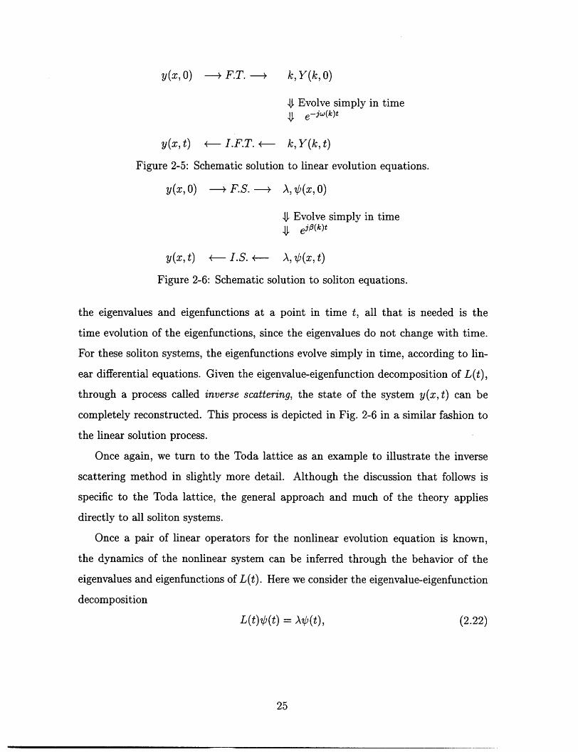
y(x, ) F.T. - k, Y(k, O)

4 Evolve simply in timee-j(k)t

y(x,t) ~ I.F.T. - k, Y(k,t)

Figure 2-5: Schematic solution to linear evolution equations.

y(x, O) > F.S. > , (x, 0)

Evolve simply in timeeij (k)t

y(x,t) I.. S A, (x, t)

Figure 2-6: Schematic solution to soliton equations.

the eigenvalues and eigenfunctions at a point in time t, all that is needed is the

time evolution of the eigenfunctions, since the eigenvalues do not change with time.

For these soliton systems, the eigenfunctions evolve simply in time, according to lin-

ear differential equations. Given the eigenvalue-eigenfunction decomposition of L(t),

through a process called inverse scattering, the state of the system y(x, t) can be

completely reconstructed. This process is depicted in Fig. 2-6 in a similar fashion to

the linear solution process.

Once again, we turn to the Toda lattice as an example to illustrate the inverse

scattering method in slightly more detail. Although the discussion that follows is

specific to the Toda lattice, the general approach and much of the theory applies

directly to all soliton systems.

Once a pair of linear operators for the nonlinear evolution equation is known,

the dynamics of the nonlinear system can be inferred through the behavior of the

eigenvalues and eigenfunctions of L(t). Here we consider the eigenvalue-eigenfunction

decomposition

L(t)4(t) = Aop(t), (2.22)

25

the n-th row of which corresponds to

(L(t)p(t))n = an l(t)b(n- 1,t) + bn(t),/(n,t) + an(t)p(n + 1,t) = Ab(n,t). (2.23)

The eigenfunctions satisfy,

d(n, t') = B(t);b(n, t), (2.24)dt

the n-th row of which yields,

d = an- 1 (t) b(n - 1,t) - a(t) (n + 1, t). (2.25)dt

Assuming that the lattice is at rest (an = 1/2 and bn = 0) for Inl > 1, the

eigenvalues of L(t) consist of a continuum A e [-1, 1], and a finite set of discrete

eigenvalues Akl > 1. The corresponding eigenfunctions can be specified in terms of

their asymptotic behavior in the regions where the motion on the lattice vanishes.

Specifically, the eigenfunctions (k(n, t) corresponding to the discrete eigenvalues Ak

are specified as

(k(n, t) - ck(t)Zn, n -+ oo, (2.26)

where zkI < 1 and Ak = (zk + zk')/2, with

00

((k (nt))2 = 1. (2.27)n=-oo

The eigenfunctions 4p(n, t) corresponding to the eigenvalues A in the continuum are

specified as

;/(n, t) - z - n + R(z, t)zn, n -+ oo, (2.28)

z-n0p(n, t) ( n -* -oo, (2.29)azt)

for A = (z + z-')/2.

We can now solve the initial value problem for the Toda lattice. Given yn(O),

the initial eigenvalue-eigenfunction decomposition can be found for L(0). The collec-

26

tion of discrete eigenvalues and the asymptotic description of both the discrete and

continuous eigenfunctions are often referred to as the nonlinear spectrum for soliton

systems. Here our nonlinear spectrum consists of

S(A, 0) = [{(zk, Ck(0)): 1 < k < N}, R(z, 0), a(z, 0)]. (2.30)

From (2.25), the time evolution of the nonlinear spectrum can be expressed as

Ck(t) = ck(O)e3k, 3k = (Zk -Zk)/2 (2.31)

ca(z,t) = e(z, 0), (2.32)

R(z, t) = R(z, O)e2 t, 3 = (z -1 - z)/2 (2.33)

which yields the nonlinear spectrum at time t, S(A, t). The inverse scattering problem

is then to reconstruct the state of the system, an(t), and bn(t) at time t, given S(A, t).

From the nonlinear spectrum, we can define the following function,

N 1F(n, t) = C ck(t)Zk + 2 f R(z, t)zn-ldz. (2.34)

k=1

We then seek a solution K(n, m, t) to the Gel'fand-Levitan-Marchenko (GLM) equa-

tion,

00

r(n,m,t) + F(n + m,t)+ E r(n,n',t)F(n' + m,t) = 0, m > n, (2.35)n' =n+l

where,00

K(n, n, t)- 2 = 1 + F(2n, t) + , n(n, n', t)F(n' + m, t), (2.36)n'=n+l1

and

r.(n,m,t)= (n, t) (2.37)

K(The GLM equation form a linear discrete-in, t m, t).The GLM equation form a linear discrete-integral equation in the terms r,(n, m, t).

27

The solution yn(t) can then be found from

an(t) = K(n + 1, n + 1, t) (2.38)2K(n, n, t)'

bnW (n, 1,) =_ K(n 1, n, t)2K(n, n, t) 2K(n - 1, n - 1, t)'

The forces on the springs, f(t), can be obtained directly

f~(t) = [K(n- 1, n- 1, t) -1. (2.39)

For a large class of soliton systems, the inverse scattering method generally in-

volves solving either a linear integral equation or a linear discrete-integral equation.

The general form of the GLM equation follows that for the Toda lattice. Although

the equation is linear, finding the solution of the GLM is often very difficult in prac-

tice. However, when the reflection coefficient, R(z), is zero, then Eq. (2.35) reduces a

set of simultaneous linear equations. This corresponds to a solution made up of pure

solitons, one soliton for each discrete eigenvalue. Examples of this method for the

Toda lattice are carried out for a single soliton and a multi-soliton solution as well as

a solution with a single pole reflection coefficient in Appendices 2.A-2.C.

2.3 Other Systems Exhibiting Solitons

Since the discovery of the inverse scattering method for the solution to KdV, there

has been a large class of nonlinear wave equations, both continuous and discrete, for

which similar solution methods have been obtained. In most cases, solutions to these

equations can be constructed from a nonlinear superposition of soliton solutions. For

a comprehensive study of inverse scattering and equations solvable by this method,

the reader is referred to the text by Ablowitz and Clarkson [1]. We briefly mention a

few to indicate the rich class of such equations.

28

1. The sine-Gordon equation

- tt = sin(O). (2.40)

The sine-Gordon (SG) equation has been used as a model for a variety of phys-

ical phenomena including the propagation of crystal dislocation [57] and the

propagation of magnetic flux along a Josephson strip line [56]. A simple phys-

ical model can be constructed by hanging pendula from an elastic line - the

angular displacement of the pendula are approximately governed by the SG

equation. A soliton solution is given by

p(x, t) = 4tan-1 e V -2, (2.41)

which is often called a "kink" soliton since it corresponds to a change in phase.

An inverse scattering solution for the SG equation has been developed by

Ablowitz, Kaup, Newell, and Segur [1].

2. The Nonlinear Schr6dinger Equation

iut + ux- ± klul2u = 0. (2.42)

The most widely-known application of the nonlinear Schr6dinger (NLS) equa-

tion has been to describe the propagation of lightwave pulses along nonlinear

fiber-optic cables [23]. Other applications include the propagation of heat in

solids, and Langmuir waves in plasma [57]. The NLS equation admits envelope

solitons of the form

u = u0sech (/k2uo(x - vet)) ei(ve/2)( -vct), (2.43)

where ve and v0 are the envelope and carrier velocities respectively [57]. The

inverse scattering solution to the NLS equation was given by Zakharov and

Shabat [79].

29

3. The Discrete-KdV Equation

un = e- eUn+. (2.44)

The discrete-KdV (dKdV) equation was discussed by Kac and Van Moerbeke

in relation to the Toda lattice. Manakov also studied the dKdV lattice for its

relation to a model for Langmuir oscillations in plasma. An inverse scattering

theory for dKdV was developed by each independently in [33] and [45]. Manakov

presents the single soliton solution for Nn = eUn,

cosh(v(n- xo- 2)) cosh(rl(n- xo + 1)) (2.45)N (t) cosh((n - x - 1)) cosh(7(n - xo))(2.45)

where

xo(t) = xo(O) + h(7)t. (2.46)

4. Cellular Automata

A number of fully-discrete dynamic systems, or cellular automata (CA), have

been shown to possess solutions with many of the properties of solitons. Ablowitz

et al. have shown several automata that possess soliton-like solutions which are

remarkably similar to the solitons of KdV or the Toda lattice [1, 52] as shown in

Fig. 2-7. Park, Steiglitz and Thurston have also observed soliton-like behavior

in automata, and even suggested possible computational applications of such

systems [53, 63, 62]. Takahashi has presented a CA similar to the automata

of Ablowitz et al., which also not only possesses soliton-like solutions, but also

has an infinite number of conserved quantities, a property shared by solvable

nonlinear systems [66].

2.4 Soliton Hierarchies

In this section we mention a few of the techniques that can be used to construct

families of solvable nonlinear evolution equations. Since we shall see that the soliton

30

eaEZ

2

Cell Number

Figure 2-7: Soliton-like solutions to the automata of Ablowitz et al.

solutions of such systems are potentially useful for communication, there may be a

practical use for the generation of increasingly complex soliton systems.

Many solvable nonlinear evolution equations, including the Korteweg-de Vries and

nonlinear Schr6dinger equations, can be written in the form

du(x, t) = K(u), (2.47)dt

where K(u) may be a function of u and its x-derivatives. In [42], Lax demonstrated

conditions under which the eigenvalues of a self-adjoint linear operator L, parameter-

ized by u, would remain invariant under time evolution of u(x, t) and hence, of L(t).

This is the so-called Lax equation, L = BL- LB, where B is an anti-symmetric

operator.

In many cases this leads directly to an inverse scattering framework, from which

the nonlinear evolution equations can be solved. Unfortunately, given a nonlinear

evolution equation, there is no constructive means known to generate a Lax pair

for the system or even to tell if one exists. Lax does indicate in [42] how given an

operator, L, an associated operator B may be constructed such that the resulting

nonlinear evolution equation is nontrivial. Although such evolution equations have

31

often been discounted for having no physical analog, such equations clearly can be

used in the signal processing contexts discussed in this thesis either through numerical

integration or with the aid of high-speed nonlinear circuitry.

A similar technique was applied to the matrix L(t) for the Toda lattice, viz.,

L[n, m] = an-ln,m+l + bndn,m + an(n+l,m, (2.48)

by Moser in [48]. Here, the evolution equation will be defined in terms of L; hence

we require BL - LB to be a tridiagonal symmetric matrix yielding the evolution of

the parameters, an(t) and bn(t). A Toda lattice hierarchy can be found by specifying

an algorithm for selecting the antisymmetric matrix, B, though the calculations are

cumbersome. The first of such matrices would be the simple matrix,

B1 [n, m] = cn-ln,m+l - Cnn+l,m, (2.49)

which leads to the following set of evolution equations,

an = an(bn - bn+1) (2.50)

b = 2c(a_ 1 - a).

With c = 1, Eqs. (2.50) are the Toda lattice equations.

The next in the Toda hierarchy can be found by allowing the matrix B to be a

penta-diagonal matrix,

B 2[n, m] = dn-2Jn-2,m + Cn-l1n-l,m - Cn6 n+l,m - dnn+2,m. (2.51)

This leads to the following set of evolution equations,

2~~~~ 2= an(an_ -an+ + bn - bn+l) (2.52)/, = 2(an..(bn1 + b) - (bn + b.+l)).

32

This higher order lattice equation contains the discrete-KdV equation as a special

case, when bn = 0, reduce to

a = an(a2 1 - a2) (2.53)

Defining an as

as = n~e/2,2= 2(2.54)

leads to the discrete-KdV equation,

in = (eUn- - eun+1'). (2.55)

This system has been studied by Moser in [48]. The inverse scattering solution for

this system was given by Manakov for the infinite line case in [45], and Kac and van

Moerbeke in [33] and [34] for both the semi-infinite and periodic cases. Though little

emphasis has been placed on this system, since it has no physical analog (though

Manakov suggests a relation to the spectra of Langmuir oscillations in plasma [45]),

realizations of the discrete-KdV system may implemented either numerically or with

analog circuits making the system of potential use in the signal processing contexts

discussed in this thesis. In Chapter 3, we show both a single circuit implementation

of this system, along with an implementation using two Toda lattice circuits based

on a relationship suggested by Kac and van Moerbeke [33] and [68].

As the number of nonlinear evolution equations solved using the inverse scattering

method grew, more methods for generating hierarchies of nonlinear equations solvable

by inverse scattering were developed. Ablowitz, Kaup, Newell, and Segur, developed

a framework for generating large classes of nonlinear evolution equations solvable

by inverse scattering [1]. This method is a generalization of the ideas of Lax, and

centers around a more general form of eigenvalue problem. For further information,

the reader is referred to [1], and [49] and the list of references therein.

33

2.A A Soliton Solution

The discrete integral equation, or GLM, is often difficult to solve, except under certain

interesting conditions. Specifically, for the case when the reflection coefficient vanishes

identically, R(z, t) = 0, the GLM reduces to a set of linear equations which can be

solved by simple methods. The only eigenfunctions that result in this case are those

corresponding to discrete eigenvalues.

We consider first the case when the solution has no contribution from the contin-

uous eigenvalues, R(z) = 0, and has only a single term from the discrete spectrum,

which we write,

z = ie -7 . (2.56)

That z can be taken as real comes from the symmetric assumption on L(t). We com-

plete the specification of the solution by selecting the initial value of the normalization

coefficient, co(O). By forming the function,

F(m, t) = cozo, (2.57)

where co = co(O)e 3°t , and o = sinh(y).

The GLM equation can now be written as

00

c(n, m) + cOoz+m + cozo' E ri(n, n')zo = 0. (2.58)nh=n+1

Following [15], (2.58) can be solved by assuming a solution of the form,

n(n, m) = Ancozo, (2.59)

leading to

n= -coA 1 + 26()v (2.60)

where

= co(t) = ea_

+ t

e = I~ = e (2.61)1 - z

34

Substituting (2.59) into (2.38), after some manipulations, we have

e-(n-qn-) - 1 = /32sech 2 (yn - 30t- 60). (2.62)

This corresponds to a single soliton solution whose direction of propagation is deter-

mined by the sign of /0, and hence the sign of z0.

2.B Multi-soliton Solutions

Once again, we consider the case where R(z) = 0, and for the discrete spectrum, we

allow N eigenvalues corresponding to z1, .. , ZN. In this case the function F(m) in

the GLM is given by,N

F(m)= Zc z. (2.63)Cj 3j=l

This results in the GLM

N 00 Nn(n, m) = C2zn+m + ,(n, n') czn+m 0 (2.64)

j=1 n'=n+l j=1

By assuming a solution of the form

N

r(n, m) = Aj,ncjz, (2.65)j=1

and substituting into (2.64), for each n, after some algebra, we have a set of N linear

equations for the N unknowns Ajn,

N ((ZZ)n+l

E 6, + ciJ Ai,n =-Cjjn, (j = 1 , N). (2.66)i= 1 - zizj ' '

This can be written in matrix form,

Aln -Cz

B(n) . , (2.67)

AN,n -CNZN

35

which lead to a direct formula for the soliton solution,

e ( q -qn- ) - 1 = IB(n)IIB(n- 2) 1.

IB(n-1)12 (2.68)

2.C Single Pole Reflection Coefficient

We now consider an example when the reflection coefficient contains a single pole in

the z-plane, at z = y, e.g,-

R(z) =1 - 7yz - l' (2.69)

where -y > 0, and c are constants. Since the discrete spectrum contains zeros of a(z),

there must be at least one discrete eigenvalue corresponding to the eigenfunction

(z) i c, n -4 oo. (2.70)

From the definition of the function F(m), we have

1F(m) = cfm + 27ri

(2.71)z Ml- dz.i1 - - x-

By the Cauchy residue theorem, the integral on the right hand side evaluates to

1 - C zm-ldz = -Crymu[mb]

27ri 1 -yz - 1

where u[m] is the discrete unit-step function. This results in

F(m) = ci mu[-m- 1].

The resulting GLM for this nonlinear spectrum is given by

(2.72)

(2.73)

00

r(n,m)+cTn+mu[-(n+m)-1]+ En' =n+l1

(n, n')cTyn +mu[-(n' +m)-1] = 0,

36

m> n.

(2.74)

For the diagonal terms, n = m, we have

K(n, n) -2 = 1 + cy 2n u[-(2n) - 1] +00

] i(n, n'/)cn'+'nu[(n' + n)- 1].n'=n+l

From (2.74) we see immediately that

r,(n, m) = 0, n+m>O.

For n + m < 0, we have

-m-1

,(n, m) + yn+m + - r,(n, n')Cyn'+m = 0,n'l=n+l

m > n. (2.77)

One method of solving (2.77), is to take the first difference with respect to m,

resulting in

n(n, m + 1) - K(n, m) + yn+M(Y - ) +-(m+1)-1

n'=n+l

/•(n, nI)Cyn'+m+l-m-1

- (4n, n)Cyn' +m = ,n' =n+l

which leads to

c(n, m + 1) - (n, m) + c'yn+m(Oy - 1) +

-m-1 (E Kc(n, n)cA n }+

n'=n+lJ

By substitution, we arrive at

k(n, m + 1)- n(n, m) + yn+m ('y- 1) + (-ic(n, m)-cyn+m ) (y- 1)- (n, -m- 1)c = 0,

(2.78)

which is solved if c = 1 - y and K(n, m) = (y - 1)/'y. Using these values in (2.75),

37

(2.75)

(2.76)

-

(-y - 1 - r,(n, -m - 1)c = .

yields

(O, n>0K(n, n) = , (2.79)

V2 =-y n <

0,O n+m > 0K(n, m) = { (-) i) nm (2.80)

(_ y_~ n+m < 0.

The initial condition that led to this one pole nonlinear spectrum is given by

1 ______-_____n 2 - [n + 1] (2.81)

2 2')

b = 0+ (1- 'y)(2 7' - 1) [n] (2.82)2-y2

which is a localized perturbation to the lattice at rest. Even for small disturbances,

1OY < 1, we see that the localized perturbation gives rise to both continuous and dis-

crete components of the spectrum. In [16], Flaschka demonstrates that any localized

disturbance must give rise to both continuous and discrete components.

38

Chapter 3

New Electrical Analogs for Soliton

Systems

Since soliton theory has its roots in mathematical physics, most of the systems stud-

ied in the literature have at least some foundation in physical systems in nature. For

example, the KdV equation was developed to describe the dynamics of small ampli-

tude surface water waves, and a large class of weakly nonlinear systems have been

demonstrated to reduce to KdV in a variety of physical applications. Such systems

range from ion-acoustic waves in plasma [78], to pressure waves in liquid gas bubble

mixtures [57]. As a result, the predominant purpose of soliton research has been to

explain physical properties of natural systems. In addition, there are several exam-

ples of man-made media that have been designed to support soliton solutions and

thus exploit their robust propagation. The use of optical fiber solitons for telecom-

munications and of Josephson junctions for volatile memory cells are two practical

examples [56, 57].

Whether its goal has been to explain natural phenomena or to support propa-

gating solitons, this research has largely focussed on the properties of propagating

solitons through these nonlinear systems. In this thesis, we take a decidedly different

perspective. We view solitons as signals and consider exploiting some of their rich

signal properties in a signal processing or communication context. This perspective

is illustrated graphically in Fig. 3-1, where a signal containing two solitons is shown

39

A

Figure 3-1: Two-soliton signal processing by a soliton system.

as an input to a soliton system which can either combine or separate the compo-

nent solitons according to the evolution equations. From the "solitons-as-signals"

perspective, the corresponding nonlinear evolution equations can be viewed as spe-

cial purpose signal processors that are naturally suited to performing complex signal

processing tasks such as signal separation or sorting. As we shall see, these systems

also form an effective means of generating soliton signals.

Although many soliton systems are described by partial differential equations, the

concept of performing signal processing operations with partial differential equations,

or wave equations, is not new. For example, signal generation and detection in pulse

compression radar systems can be accomplished using a dispersive delay line [61].

Such systems can be constructed either using bulk material, like a surface acoustic

wave (SAW) device, or with a lumped element line. In either case, a signal is induced

into the device and allowed to propagate according to the wave equations that describe

the device. Once the signal has propagated along the device and the appropriate delay

or other processing has been accomplished, the signal can be extracted from the

medium. SAW devices can also be used for a variety of signal processing applications

including chirp Z-transforms or digital filtering [11].

In this chapter, we study circuit implementations of two of the nonlinear evolution

equations discussed in the previous chapter. The first of these is a nonlinear LC

ladder network developed by Hirota and Suzuki [29]. Although this circuit serves

as a useful electrical model for the Toda lattice, it is difficult to implement using

standard components. We present a new circuit model for the Toda lattice based on

a precise electrical analog of the exponential spring mass system. This circuit has

40

10.

- - - __JL/\',____0_fA��

L L L L L

V.(t *-00 :4 in()< V .7 V257 -~ v 7-v 1t

Figure 3-2: Nonlinear LC ladder circuit of Hirota and Suzuki.

been implemented in hardware using standard components and appears to be the first

such circuit to display true soliton behavior. We also present a new circuit model for

the discrete-KdV equation, for which there is no prior electrical or mechanical analog.

3.1 Toda Circuit Model of Hirota and Suzuki

Motivated by the work of Toda on the exponential lattice, the nonlinear LC ladder

network implementation shown in Fig. 3-2 was given by Hirota and Suzuki in [29].

Rather than a direct analogy to the Toda lattice, the authors derived the functional

form of the capacitance required for the LC line to be equivalent. The resulting

network equations are given by

(2 V.() 1d-n -+ (Vn-1 (t) - 2V(t) + V+(t)), (3.1)dt2 k V 0 ) LoVo

which is equivalent to the Toda lattice equation for the forces on the nonlinear springs

given in Eq. (2.12). This amounts to an implicit mapping from force to voltage,

f (t) -+ V(t). The capacitance required in the nonlinear LC ladder is of the form

cy 0C(V) = Vco +VO (3.2)

where V0 and Co are constants representing the bias voltage and the nominal capac-

itance, respectively. In their implementation, varactor diodes with nonlinear capaci-

tance

C(V) 27(V- Vb)- 48pF, (3.3)

41

where Vb is a bias voltage, were used to approximate the required capacitance of

Eq. (3.2).

Although the varactor diode capacitance can be biased to yield a fairly good

match for small voltages, for larger voltages, the deviations from the ideal capacitance

becomes apparent. Moreover, as the length of the lattice increases, the effects on any

propagating solitons accumulate. The net result is that interaction between solitary

waves of appreciable amplitude will not result in soliton collisions; rather such a

collision will also produce a nontrivial amount of ripple [29]. Also, since the circuit

is only accurate for small voltages, where the velocity difference between solitons is

small, large numbers of nodes are required to bring about collisions.

After publication of their circuit [29] and subsequent publication of modulation

experiments using the circuit [64, 65], several papers have appeared in the literature on

a variety of related topics. In [39], Kolosick et al. analyze a similar nonlinear network.

In [32] Islam, Singh and Steiglitz studied the effects of dissipation on the propagation

of individual solitons as well as the interaction of pairs of solitons. They found

that dissipative effects led to a decrease in amplitude and an increase in the width

of solitons as they propagate through the lattice. These findings are in agreement

with the numerical work of Okada, Watanabe and Tanaca in [50], whose studies

showed similar effects due to parameter fluctuation in the periodic Toda lattice. In [4]

Ballantyne et al. observed the Jacobian elliptic function solutions in a periodic version

of the nonlinear LC line. Toda also demonstrated properties of the nonlinear line and

illustrated the existence of modulated solitons, by relating the lattice to the nonlinear

Schrbdinger equation in [68]. Finally, Cho, Wakita and Miyigawa developed a similar

nonlinear network as an equivalent circuit model for the propagation of nonlinear

surface acoustic waves in thin-bar and broad-plate vibrations. They also have shown

that the nonlinear LC network is an accurate model for a metallic grating waveguide

and use this circuit model to explain certain nonlinearities observed in SAW devices

including the generation of acoustic phase conjugate waves [10].

42

il i2 in in+1-~ - ~ -~ -

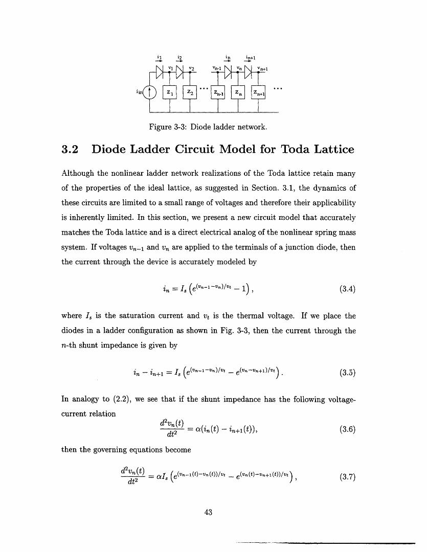
Figure 3-3: Diode ladder network.

3.2 Diode Ladder Circuit Model for Toda Lattice

Although the nonlinear ladder network realizations of the Toda lattice retain many

of the properties of the ideal lattice, as suggested in Section. 3.1, the dynamics of

these circuits are limited to a small range of voltages and therefore their applicability

is inherently limited. In this section, we present a new circuit model that accurately

matches the Toda lattice and is a direct electrical analog of the nonlinear spring mass

system. If voltages v,_i and v, are applied to the terminals of a junction diode, then

the current through the device is accurately modeled by

in = s (e (V" - - V) / t - 1), (3.4)

where 1S is the saturation current and t is the thermal voltage. If we place the

diodes in a ladder configuration as shown in Fig. 3-3, then the current through the

n-th shunt impedance is given by

in-in+1 = I. (e(V,-I-vn)/Vt - e(Vn-"n+1)/Vt) (3.5)

In analogy to (2.2), we see that if the shunt impedance has the following voltage-

current relation

d(t) = (in(t) - in+ (t)), (3.6)

then the governing equations become

dt2V() = I (e(vn-1(t)-vn(t))/vt - e(vn(t)-vn+1(t))/vt) (3.7)dt2

43

Figure 3-4: Double capacitor circuit diagram.

or,

- In 1 + j (in-1 (t) - 2in(t) + in+ 1 (t)), (3.8)dt2 / Vt

where i (t) = i(t). These are equivalent to the Toda lattice equations with a/m

aI, and b = 1/vt. The required shunt impedance is often referred to as a dou-

ble capacitor, which can be realized using ideal operational amplifiers in the gy-

rator circuit shown in Fig. 3-4, yielding the required impedance of Zn = a/s 2 =

R 3/RR 2C 2s 2 [30, 59].

When i(t) in Fig. 3-3 is of the form

iin(t) = If 2 sech 2(_yt), (3.9)

a single soliton is induced in the line resulting in

in(t) = Isf]2 sech2 (pn - fyt), (3.10)

where fQ = sinh(p). Note that the saturation current I may be absorbed into the

parameter Q, yielding

in(t) = fi2 sech2 (pn - /3 T), (3.11)

where /3 = v~ sinh(p), and T = ta/vt. Since Is is generally on the order of pico-

amps, the operating range of the circuit can be on the order of milliamps over a wide

44

range of values of the soliton wavenumber p. As a result, the diode ladder circuit

model is very accurate over a large range of soliton wavenumbers, and is significantly

more accurate than the LC circuit of Hirota and Suzuki.

Solitons of the form of Eq. (3.11) are solutions of the infinite-length Toda lattice

equations. In practice, a finite-length lattice can be constructed to yield soliton solu-

tions if the diode ladder circuit can be appropriately terminated to limit reflections.

As a starting point, we consider the termination that would yield no reflections for

the small signal model. This can be obtained from the impedance of the line when

the diodes are replaced with their equivalent linearized resistance Req = vt/id, where

id is the current in the linearized diode. This results in an impedance

Zin q + 4 q (3.12)2 82

For typical component values, oa 1011. If Req is taken to be vt/25mA = 1, then for

frequencies below 1 MHz, a load impedance consisting of a 1Q resistor and a 0.31LF

capacitor approximate Eq. (3.12) well and yield negligible reflections in practice.

3.3 Circuit Simulation

The diode lattice has been simulated using realistic component models in the circuit

simulation package HSPICE [47]. The diodes used are model ln4148 with a saturation

current of I, x .OlpA. Setting the operation range of the circuit to produce solitons

on the order of lOmA yields a value of p - 14. To fix the time scale of the circuit, we

set the pulse width of a soliton to approximately 5us, which leads to

sinh(p) / 5 (3.13)

or a - 1011. The resistor values in the double capacitor circuits can now be chosen to

prevent saturation of the operational amplifiers. By calculating the transfer function

from the driving point of the double capacitor to each of the operational amplifier

45

output voltages, we obtainR2 + R3

G1 R ' (3.14)

R 2 + 2R 3G2 = 1 + R RCs, (3.15)

where G1 and G 2 are the transfer characteristics from the voltage vn to the outputs

of the top and bottom amplifiers, respectively. In order to select a valid set of resistor

values, the range of voltages seen at the top of the double capacitor is needed. For a

single soliton solution, the closed form solution for the voltage is

vn(t) = vt In {cosh (p(n)- /3t V )}- vt In {cosh (p(n + 1) - /3taV) } + const.

(3.16)

The limiting voltage in Eq. (3.16) is given by

lim vn(t) = vtp + constant, (3.17)t-+o0

and

lim v(t) = -vtp + constant. (3.18)t-+-00

Selecting the constants such that vn(-oo) = 0, gives

lim vn(t) = 2 vtp. (3.19)t---oW

For p - 14, this leads to a final voltage amplitude on the order of vn 0.75 volts. For

each soliton that passes through a given node, the voltage on the double capacitor

will increase by 2 vtp. In order to keep the amplifiers from saturating due to a single

soliton, G1 and G 2 must remain less than about a factor of 10. Since each soliton that

passes through a given node will result in a similar voltage increase, we would like

these gains to be as small as possible to avoid saturation. However, it is also important

to maintain voltages levels in the double capacitors that are above the noise level for

the circuit, which implies that these gains cannot be too small. A reasonable balance

can be obtained by setting R 2 ~ R 3 , and R < 1/C which can be met by selecting

46

20(mA) :

(mA)

(mA)

(mA)

10 -

n~ ,

IEU 20

10

20

10

0 11 1 111 ... 1 0 ,20-I10~~~~~~~~~~~~~~~~~~~~~~~~~~~~~~~~~~~~~~~~~~~~~~'°0

diode5

diode4

diode3

diode1

0 100 200 300 400 500(As)

Figure 3-5: HSPICE simulation of the evolution of a two-soliton signal through thediode lattice. Each horizontal trace shows the current through one of the diodes 1, 3,4and 5.

R = R2 = R3 = kQ and C = .01LF. These values permit soliton pulse widths

of about 5/s with amplitudes of about 10mA and with voltages at the amplifier

outputs within the double capacitors on the order of 1 Volt. The double capacitors

use precision LT1028A operational amplifiers with a gain bandwidth product of about

65 MHz. Shown in Fig. 3-5 is an HSPICE simulation with two solitons propagating

down a length 10 Toda chain.

A significant difference between soliton solutions to this circuit and those of the

nonlinear LC line lies in the scale of operation. Due to biasing constraints for the

LC line, solitons were generally restricted to a small range of wavenumbers in the

neighborhood of p . 1. Over this range, the propagation velocity of the solitons,

which is proportional to sinh(p)/p does not vary greatly between solitons of different

wavenumbers. This led to the use of chains with hundreds of nodes in order to demon-

strate soliton collisions. The diode ladder circuit, however, can operate in the range

p - 14 for solitons with amplitudes in the mA range. Due to the exponential nature

of the sinh function, the velocities of solitons with slightly different amplitudes for

currents in the mA range yield exponentially different velocities. This enables soliton

47

. . .

collisions to take place with far fewer nodes than with the nonlinear LC network.

As illustrated in the bottom trace of Fig. 3-5, a soliton can be generated by

driving the circuit with a square pulse of approximately the same area as the desired

soliton. As seen on the third node in the lattice, once the soliton is excited, the non-

soliton components are quickly stripped away. For the example in the figure, a small

pulse followed by a larger pulse are used to drive the circuit giving rise to a small

soliton followed by a larger amplitude soliton. This property has been demonstrated

experimentally for a number of soliton systems, c.f. [23] for the nonlinear Schr6dinger

equation and [29] for the Toda lattice. It has been shown theoretically for KdV, c.f.

[1] and [12], that practically any smooth, localized disturbance of the proper area will

result in a soliton with that area, if such a solution exists. Multi-soliton signals could

also be generated by using inverse scattering techniques to determine a drive signal

iin(t) that would give rise to the desired solitons. However, this method requires more

complex drive circuitry than simple pulse generators.

Note that as the faster soliton overtakes the slower as viewed on the fourth node

in Fig. 3-5, the joint signal amplitude is significantly less than the sum of the indi-

vidual amplitudes. Also, the signal shape changes significantly during the nonlinear

interaction. These two effects will impact both the energy of multi-soliton signals and

the ability to recover their signal parameters.

3.4 Circuit Implementation

To perform real-time experimentation and to verify the operation of the model using

standard components, the diode ladder circuit has been implemented in hardware.

Real-time implementation also enables rapid testing of soliton processing techniques

and enables measurements of actual circuit noise levels. Such noise measurements

permit experimental verification of some of the theoretical results we obtain in Chap. 5

concerning system noise.

In the construction of the circuit, there were several practical matters to be dealt

with. First, the diode ladder is driven by a current source. In our implementation

48

100 kQ

vl

v2

100 kQ

(vl-v2)

1000

Figure 3-6: Precision bipolar current source.

the precision bipolarity current source shown in Fig. 3-6 taken from [30] was used.

When implemented with the low noise LT1028A operational amplifiers, this circuit

provides a reliable, accurate current source, with low leakage. In practice, leakage

current turns out to be a problem, since the double capacitor circuits are marginally

stable. The node voltages are double integrators of their current and therefore any

excess current will lead to large deviations in the node voltages and corrupt soliton

propagation.

In addition to the voltage deviations from leakage current, each soliton that passes

through a node on the ladder contributes a net voltage increase of 2vtp or approxi-

mately Volt. Therefore a signal containing three solitons will leave the node with

a net voltage increase of nearly 3 volts. If several such signals are processed by this

circuit, the operational amplifiers in the double capacitors will eventually saturate.

This problem can be overcome by resetting the node voltages after each signal has

been processed by the circuit using analog switches as shown in Fig. 3-7.

Finally, since the solitons are present in the diode ladder circuit as current wave-

forms, there must be an adequate means of measuring the current through the diodes

without significantly affecting the dynamics of the circuit. This can be accomplished

by placing a small resistance in series with each diode in the lattice a shown in Fig. 3-

7. The current through the diodes can then be observed by measuring the voltage

drop across each of the resistors with a differential amplifier.

A hardware implementation of the diode ladder circuit with twelve nodes is shown

49

Figure 3-7: Diagram for the double capacitors used in the diode ladder circuit. Analogswitches, placed in parallel with the capacitors, are used to reset the circuit after eachprocessed signal.

in Fig. 3-8. Each of the three rightmost bread boards in the figure contains four stages

of diodes, series resistors, and double capacitors. The left most bread board con-

tains pulse-generation circuitry, and the remaining bread board contains the voltage-

controlled current source. A two-soliton signal generated by this circuit is shown on

the oscilloscope traces in Fig. 3-9. The bottom trace in the figure corresponds to the

input current to the circuit, and the remaining traces, from bottom to top, show the

current through the second, third and fourth diodes in the lattice.

For a more complex example, a simple waveform consisting of three component

soliton signals, periodically repeated, was used to drive the diode ladder circuit with

several additional stages. Using a digital oscilloscope to sample real-time circuit

waveforms, measurements of the diode currents were transferred to a computer, and

then plotted online. The measured currents through each of the diodes are shown in

Fig. 3-10. The time axis of the figure is such that t = 0 corresponds to the beginning of

a period. The largest amplitude soliton measures 17mA, with a pulse width of 82,/s at

the first node. As measured on the fifteenth node, the amplitude is 14mA with pulse

width of 86us. This decay in the soliton amplitude is on the order of 1% per node

50

Figure 3-8: Hardware implementation of the diode ladder circuit. The first columnfrom the left contains the pulse-generation circuitry; the second contains the voltage-controlled current source; each of the last three contains four stages of diodes, seriesresistors and double capacitors.

51

Figure 3-9: Oscilloscope traces for two solitons in the diode ladder circuit. The tracescorrespond to the currents in the first four diodes.

and may have several causes in addition to deviations of the circuit components from

their idealized models. Specifically, as stated in [32], dissipative effects in the lattice

are contrary to the conservative nature of the Toda lattice, and will necessarily lead

to energy loss. Also, as shown in [50], inter-node parameter fluctuations can lead to

dispersion, causing decay as well as additional non-soliton components. This leads to

a change in the soliton parameter 3, resulting in a decrease in soliton velocity as they

propagate through the lattice. In the figure, there is also a small spike that appears

in each of the diode currents near the time t = -ms. This results from the reset

signal, Vsw, propagating down the lattice and resetting adjacent double capacitors at

slightly different times.

3.5 Circuit Model for Discrete-KdV

The discrete-KdV equation (dKdV), sometimes referred to as the nonlinear ladder

equations [1], or the KM system (Kac and vanMoerbeke) [67] is governed by the

52

16

14

ECa)a)'a0'0U,V_

12

10

8

6

4

2

0

_0

Diode Ladder Circuit Waveforms

-3 -2 -1 0 1 2time (ms)

3

Figure 3-10: Diode currents measured from the diode ladder circuit in operation. Theinput signal consists of three square pulses of different areas. The spike that appearsin the figure near t = -1 ms is a result of the signal that resets the lattice.

53

~~I I I I l

-I

-

L

equations,

in(t) = eun-(t) _ eun+1(t) (3.20)

This equation is first order in time, which makes the dynamics less complex than the

Toda lattice, yet as evidenced in Sec. 2.2, the inverse scattering framework is very

similar. Although much of the theory for this nonlinear system has been developed

with the theory for the Toda lattice, the discrete-KdV equations are generally ignored

since there is no clear physical analog of these equations. However, there is special re-

lationship known as a Biicklund transformation which provides a connection between

this system and the Toda lattice [67, 33, 34].

Given our success with the Toda lattice using a ladder comprising diodes and

double capacitors and the similarity between (3.20) and (3.7), we first consider a

ladder of diodes with shunt capacitors. A similar analysis leads to the following set

of equations

dv (t) = Is (e(nI(t)-V(t))/Vt - e(vn(t)-vn+(t))/vt) (3.21)dt CI

which look deceptively similar to (3.20). However, there is no apparent means of

decoupling the node voltage, vn(t) from v+(t) and vn_ (t) as would be required.

This similarity is not a mere coincidence and actually leads to a realization of the

discrete-KdV equation using two Toda circuits. Following [33] and [67], let

un -Rn, t -+-t, (3.22)

which transforms (3.20) to

= e - & - - e - +i. (3.23)

Letting q = R. + Rn+, then qn satisfies

qn = 2e -qn - e-qn -2 - e qn

+ 2 (3.24)

54

f f f1,n-1 1,n 1,n+1

R P/k1 2n 2+1 2n+2

f f f2,n-1 2,n 2,n+1

Figure 3-11: Illustration of the relationship between two adjacent Toda lattices,fini = 1,2 and the discrete-KdV equation. This process suggests a possible im-plementation of the dKdV equation using two adjacent Toda lattice circuits.

Taking every other term, i.e. ql,n = q2n, q2,n = q2n+l, we have

qi,n = 2e - qi n - e- qi n- - eqi ,n+ l i = 1, 2. (3.25)

Setting qi,n = -ln(1 + fi,n),) yields

d2ln(1 + fi,,n)dt2 = fin-- 2fi,n + fi,n+l i = 1, 2, (3.26)

which are each a Toda lattice equation. The physical interpretation of this transfor-

mation is the following: if fl,n and f2,n are each defined within a different Toda lattice,

then Rn defined by R 2n = fl,n- f2,n, R 2n+l f2,n+l- fl,n satisfies the discrete-KdV

equation in the form (3.23). This process is illustrated in Fig. 3-11. Although a dKdV

circuit could be so constructed, the resulting circuitry would be twice as complex as

the Toda circuit. A much simpler implementation can be found by maintaining the

aspects of the diode ladder that are useful, namely the exponential current relation-

ship of the diodes, while removing the aspects which are troublesome, viz. the ladder

interconnections.

Since the desired equations are first order, we use capacitor voltages for state

variables, i.e. vn(t) will be the voltage on the n-th capacitor. Rather than assembling

the capacitors in a ladder network, we consider a collection of nodes with nearest

neighbor coupling as shown in Fig. 3-12. Each node is maintains a node voltage, vn(t),

and also maintains a voltage that is proportional to en(t), which can be accomplished

55

.

Figure 3-12: Collection of nodes for the discrete-KdV circuit.

with a voltage follower and a diode as shown in Fig. 3-12. Since the voltage follower

mirrors the voltage on the capacitor, neglecting the voltage drop from the resistor,

the voltage across the diode is approximately vn(t). Hence the current through the

diode is i(t) - Is(exp(vn(t)/vt)- 1), where t is the thermal voltage. Since each

node maintains a node voltage along with a voltage proportional to exp(vn(t)), all

that remains is to construct a current source that is proportional to the difference

in the exponential reference voltages of the neighboring nodes. If a current source

is used to drive the capacitor as shown in Fig. 3-12, then the node voltage, v(t), is

governed by

i (t) = Is (evn-l(t)/vt - evn+1(t)/vt) (3.27)

The required differential voltage controlled current source can be the same as the one

that drives the Toda ladder circuit, shown in Fig. 3-6. Therefore, for a collection of

nodes such as those in Fig. 3-12, the node capacitor voltages are governed by the

discrete-KdV equation.

The time scale of the circuit can be set by proper choice of the ratio IS/C. Specif-

ically, if IS = avtC, the node voltage satisfies,

dv, (-r)/ vt _ _ t n+ (T)/vt) (3.28)

where = t/a. Thus vn(t)/vt satisfies the discrete-KdV equation on a time-scale t/a.

56

An HSPICE simulation of this circuit indeed verifies the propagation of dKdV

solitons. Since this circuit is first order, the state of the system is completely specified

by the capacitor voltages. Rather than processing continuous-time signals as with

the Toda lattice system, we can use this system to process discrete-time solitons

as specified by v. For the purposes of simulation, we consider the periodic dKdV

equation by setting v~+1 (t) = vo(t) and initializing the system with the discrete-time

signal corresponding to a listing of node capacitor voltages. We can place a multi-

soliton solution in the circuit using inverse scattering techniques to construct the

initial voltage profile. The single soliton solution to the dKdV system is given by

vn(t) = In cosh(-y (n- 2) - t) cosh(7 (n + 1) -fit) (3.29)cosh(-y (n - ) - t)cosh ( n - t)

where fi = sinh(2-y). Shown in Fig. 3-13, is the result of an HSPICE simulation

of the circuit with 30 nodes in a loop configuration, each with 2nF capacitors and

diodes with a saturation current chosen to be I = t x 2nA. Thus, the time scale

of the circuit is unity, a = 1. The initial condition was set such that a soliton with

y = 2.5 was placed on node 0 and a second soliton with y2 = 2 was placed on node

10. As with the diode ladder implementation of the Toda circuit, this circuit model is

very accurate, and can support a wide range of soliton wavenumbers. Discrete-time

soliton signals could be used as an initial condition to the dKdV lattice and then be

processed by their evolution in the circuit.

3.6 Further Considerations

In this chapter we have illustrated three circuits which can be used to both generate

and to process soliton signals. The first of the three, developed by Hirota and Suzuki,

demonstrated the feasibility of using such nonlinear circuits as analogs of soliton

systems. Their results [29, 64, 65], along with the experimental work of Toda in [68],

Scott in [56, 57], and a host of others illustrate the potential for development of a

variety of analog hardware for soliton processing techniques.

57

ao °1 eo o O 0 0 Go 0 ok f Voooroobt

o- Q

)XD. eetoee~ ea °° °°iT ° 4T @°0 2°°°°TJTGCD - 5 : o

0. .TT . I TT " 209 aO- -= : 1'0 1'5": ~ 0 ' ~ E ~C; ~ ~ ~ ~ ~ ? p ~ zz 5 : z i

al 5 - O Tr 9 a 911f zze e z & 0

timne (s) node index

Figure 3-13: To the left, the normalized node capacitor voltages, v(t)/vt for eachnode is shown as a function of time. To the right, the state of the circuit is shownas a function of node index for five different sample times. The bottom trace in thefigure corresponds to the initial condition.

We then presented a new diode ladder circuit which models the Toda lattice more

accurately than the nonlinear LC circuit and can be operated over a larger range

of soliton amplitudes. Increasing the range of operation has a direct impact on the

complexity of the processing hardware that would be used, for example, to separate

multi-soliton signals. Specifically, the number of nodes required (length of the lattice)

is significantly reduced. A real-time implementation of this circuit was constructed

in hardware using standard components which appears to be the first such circuit to

experimentally demonstrate true soliton collisions. It remains to be seen whether or

not the diode ladder circuit can operate without the need for periodic resetting of

the double capacitor sub-circuits. The resolution of this issue might avail the diode

ladder circuit to a greater range of potential processing techniques and is therefore

an interesting avenue for future work.

Finally, we presented a new circuit which implements the discrete-KdV equation,

for which no other circuit models have previously been presented. Experiments using

HSPICE demonstrate the viability of the circuit model for a variety of discrete-time

soliton processing techniques. As shown, the dKdV circuit is placed in a loop con-

figuration and the circuit iterates forward from an initial condition. This circuit can

also process continuous signals in an analogous manner to the Toda lattice. However,

58

co5._

:p :

5 101) o 5 - - Q- - 25 1:Os~ 0,O

the problem of properly terminating the dKdV circuit differs from its Toda lattice

counterpart due to the more complex circuit topology.

The circuits developed in this chapter can be used to generate multi-soliton signals

as well as perform a variety of processing operations. For example multiple solitons

can be multiplexed by using a signal with solitons arranged in increasing amplitude

as input, allowing them to collide, and then extracting the signal from the circuit.

Similarly the separation of multiple overlapping solitons could be achieved by allowing

them to propagate at different velocities and again extracting the signal after sepa-

ration. Each of these otherwise complex nonlinear tasks can be completed naturally

by the dynamics of the nonlinear systems. Such systems also indicate the viability

of analog hardware implementations of a large class of nonlinear systems exhibiting

soliton behavior. Additionally, many of the soliton processing techniques could be

mapped onto the soliton or soliton-like behavior that has been exhibited by a large

class of cellular automata [1, 7, 53, 62, 63, 66], for which many fast algorithms [52]

and hardware [46, 70, 71] have been developed.

59

60

Chapter 4

Communication with Soliton

Signals

Many traditional communication systems use a form of sinusoidal carrier modula-

tion, such as amplitude modulation (AM) or frequency modulation (FM) to transmit

a message-bearing signal over a physical channel. The reliance upon sinusoidal sig-

nals is due in part to the simplicity with which such signals can be generated and

processed using linear systems. More importantly, information contained in sinu-

soidal signals with different frequencies can easily be separated using linear systems

or Fourier techniques. This has led to the development of standards and regulation

of the sinusoidal composition of signals transmitted electromagnetically based on the

allocation of separate bands of frequencies to different users.

The complex dynamic structure of soliton signals and the ease with which these

signals can be both generated and processed with analog circuitry renders them po-

tentially applicable in the broad context of communication in an analogous manner

to sinusoidal signals. We have also seen that either by using analog circuitry or

the inverse scattering transform, the individual solitons in a multi-soliton signal can

also be easily separated. In this chapter we will present a paradigm for modulation

of information on soliton carriers and illustrate the potential applicability of such

a framework to multi-user communication. Specifically, we consider a scenario in

which solitons are used as carrier waveforms in an amplitude- or position-modulation

61

Figure 4-1: A soliton carrier signal for the Toda lattice.

communication system using the soliton systems to perform signal multiplexing and

demultiplexing. In this context, we will show that the signal amplitude reduction

that occurs during soliton interaction may provide increased energy efficiency, mak-

ing such techniques particularly attractive for a broad range communication contexts

over power-limited channels including portable wireless communication, satellite or

deep-space applications.

4.1 Soliton Modulation

Although the mechanisms for the generation and processing of soliton signals differs,

many standard sinusoidal carrier modulation techniques could be implemented using

soliton carriers. In this chapter, we define a soliton carrier as a signal which is

composed of a periodically-repeated single soliton solution to a particular nonlinear

system. For example, a soliton carrier signal for the Toda lattice is shown in Fig. 4-1

and can be written,

f(t) {E /32sech2 [ (n - A) - 3t] - 2v (4.1)

where a and 3 are parameters related to the elliptic functions defined in Chap 2,

Eq. (2.11). In addition to the Toda lattice, periodic soliton solutions of many soliton

systems can be written in terms of Jacobian elliptic functions as in Eq. (2.10).

As a soliton carrier such as that for the Toda lattice in Fig. 4-1 is generated,

a simple amplitude modulation scheme could be devised by modulating the soliton

parameter 3, since the amplitude of the Toda lattice solitons is proportional to /2.

Note that the pulse-width also changes with 3, giving rise to a scale modulation

62

Figure 4-2: Modulating the relative amplitude or position of soliton carrier signal forthe Toda lattice.

rather than a pure amplitude modulation. Similarly, an analog of FM/PM or pulse-

position modulation could be achieved by modulating the relative position of each

soliton in a given period, as shown in Fig. 4-2. Although the mechanisms developed

for sinusoidal carrier demodulation would also have to be adapted, at least from a

signal generation viewpoint, a variety of sinusoidal carrier modulation techniques can

be directly mapped onto soliton carriers. We have again focused on the Toda lattice

as an example, however, parameter modulation of soliton carriers could be applied to

the large class of soliton signals that can be both generated and processed by solvable

nonlinear systems.

4.2 Soliton Multiplexing

As a simple extension, the soliton modulation techniques described in Section 4.1 can

be generalized to include multiple solitons in each period and accommodate multiple

information-bearing signals, as shown in Fig. 4-3 for a four soliton example using the

Toda lattice circuits developed in Chap. 3. In the figure, a signal is generated as

a periodically-repeated train of four solitons of increasing amplitude. The relative

amplitudes or positions of each of the component solitons could be independently

modulated about their nominal values to accommodate multiple information signals

in a single soliton carrier.

The nominal soliton amplitudes can be appropriately chosen so that as this signal

is processed by the diode ladder circuit, the larger amplitude solitons propagate faster

than the smaller solitons, and each of the solitons can become nonlinearly superim-

63

\ / v.

0

Figure 4-3: Multiplexing of a four soliton solution to the Toda lattice.

posed as viewed at a given node in the circuit. From an input-output perspective, the

diode ladder circuit can be used to make each of the solitons coincidental in time. As

indicated in the figure, this packetized soliton carrier could then be transmitted over

a communication channel. At the receiver, the multi-soliton signal can be processed

with an identical diode ladder circuit which is naturally-suited to perform the non-

linear signal separation required to demultiplex the multiple soliton carriers. As the

larger amplitude solitons emerge before the smaller, after a given number of nodes,

the original multi-soliton carrier re-emerges from the receiver in amplitude-reversed

order. At this point, each of the component soliton carriers could be demodulated to

recover the individual message signals it contains. Aside from a packetization of the

component solitons, we will see that multiplexing the soliton carriers in this fashion

can lead to an increased energy efficiency for such carrier modulation schemes.

Since the Toda lattice equations are symmetric with respect to time and node

index, solitons can propagate in either direction. As a result, a single diode ladder

implementation could be used as both a modulator and demodulator simultaneously,

as shown in Fig. 4-4. From the figure at time t = 0, a signal composed of three solitons

is multiplexed by the system, by propagating the separated solitons along the lattice

from node 0 to node 35. The resulting multiplexed signal can be extracted from node

35 around t = 30. Also at t = 0, a received signal composed of three multiplexed

solitons is input to the system at node 35. These solitons are induced in the reverse

direction, allowing them to separate by the time they arrive at node 0 around t =

30. Since the forward propagating solitons correspond to positive eigenvalues in

64

. t A/IW

35

3

010

time

Figure 4-4: Toda lattice response to an outgoing signal at node 0 and to a receivedsignal at node 35, each with three component solitons. The solitons that are input atnode 0 are multiplexed by the system, as viewed on node 35. The solitons that areinput to node 35, propagate in the reverse direction, and are demultiplexed by thesystem, as viewed on node 0.

the inverse scattering transform and the reverse propagating solitons have negative

eigenvalues, the dynamics of the two signals will be completely decoupled. The ability

to propagate solitons in both directions is a property shared by many soliton systems

with dynamics governed by differential equations that are second order in time.

Although presented in the context of the Toda lattice equation, the soliton mod-

ulation techniques presented are applicable to a variety of soliton systems, both in

discrete- and continuous-time. For example, a similar technique can be used for mod-

ulation of the discrete-time solitons generated by the discrete-KdV equation. Both

the soliton amplitude and relative position for a multi-soliton solution of the dKdV

equation could be independently modulated when the solitons are well-separated in

time. This multi-soliton signal could then be used as the initial condition to a dKdV

circuit developed in Chap. 3, and then iterated forward in time until the component

solitons were mutually overlapping. This multiplexed signal could be transmitted

to a receiver where identical dKdV circuitry is used to demultiplex the component

solitons.

65

-lU

4.3 Spectrum of Toda Lattice Solitons

To draw comparisons with sinusoidal AM and FM modulation, we consider the Fourier

spectrum of a periodic single soliton carrier for the Toda lattice. We consider a

solution of the form of Eq. (4.1) for a fixed node,

00

f(t) = E 32 sech2((t- iT)) - 2/, (4.2)£=-00

where T is the period of one message frame. The Fourier transform of a single soliton

(or one frame) is given by[13]

F(w) = J v(t)e-iJ tdt-oo

7rw27r,36(w). ~~(4.3)

sinh (rw/2,3) - 2r3() (4.3)

In the small amplitude limit, the periodic traveling wave solutions to the Toda lattice

approach sinusoids. To see that this is reasonable, we consider the Fourier transform

of the periodic soliton, Eq. (4.2), which, ignoring effects due to time aliasing, is given

by00

F~~~w)=r Zw £~e=eF(w) eo sinh (rw/2) 6 (-w), (4.4)£=-oo,£:0

where wc = 27r/T. Since the Fourier series coefficients fall off exponentially in fre-

quency, for small amplitudes ( << we),

F(w) - 47r/J(w - w,) + 4r/36(w + w,), (4.5)

which is in line with the asymptotic sinusoidal form of f(t).

We now consider an AM modulation with a single soliton waveform,

fAM(t) = f(t)(1 + m(t)), (4.6)

where m(t) is the message signal. We also assume that the modulation depth is

small, i.e. the bandwidth of m(t) is much smaller than wc. To illustrate the resulting

66

spectrum, we set m(t) = m cos(wmt), which yields

E = inh (w/23) k W ) 2 (W - f + Wm + m 26( W - Wm))=-~oo~,£0sinh (ro/2) 2 2(4.7)

(4.7)

Again, making the small amplitude approximation ( < w), the positive half of the

spectrum is given by

F+(w) ~ 4irf6(w - wc) + 27rf(w - (w, - wm)) + 2irf6(w - ( + wm)), (4.8)

which is the same as the spectrum for a sinusoidal AM modulation.

In analogy to FM, we consider a soliton carrier with the relative position of the

component solitons modulated,

fFM(t) = f(t + mcos(wmt)), (4.9)

again assuming that wm << wc. This expression can be expanded using a trigonometric

identity, to

o o2fFM(t) = E M

t=-- (cosh(fre) cosh(3m cos(wmt)) + sinh(f3re)

where r = t- T.

sinh(Om cos(wmt))) 2 - 23,(4.10)

Making the assumption that m < T, this expression can be

approximated to first order in m by

00

e--oocosh 2 (fre)+ 2 cosh(rte) sinh(fre)m cos(wmt)-203

00

E /32 sech 2 (fire) - 2/32sech 2 (3re) tanh(/3re)mcos(wmt) - 2f(4.11)i=-oo

Noting that

d32 sech (pt) = -2,3 3sech2 (/t) tanh(/it),dt

(4.12)

67

FAM(W) =

fFM(t)

we obtain the approximate Fourier transform of fFM(t) as

FrW jr(w - m)2 /2 j7r(w + W) 2 /2FM ) sinh (w/2/) sinh (r(w - Wm)/2/) sinh (r(w + wm)/2)' (4.13)

Again, making an approximation for 3 < 1, and noting that in the limit of small

/3, the period T of the signal must approach , the positive half of the spectrum is

approximated by

VFM,+(w) - 47r/36(w - we) + j2r/36(w - (we - wm)) + j2r/3(w - ( + wm)), (4.14)

which has the same magnitude as the spectrum for a sinusoidal AM modulation, and

is the same spectrum that would be obtained by sinusoidal FM modulation.

For the two-soliton signal, from Chapter 2, Eq. (2.6), a single period of the signal

is of the form

,/3sech2 (1) + /32sech2 (7 2) + Asech 2(l 1)sech 2 (7 2)f(t) = (cosh(0/2) + sinh(q/2) tanh(yl) tanh(2))2 (4.15)

with qi = /3i(t- i). Thus, for positional modulation, 6i = mi(t), in addition to

the spectral components of the individual messages, there is a contribution from

the product of the individually modulated solitons. However, when the solitons do

not overlap, A - 0 and the modulation is essentially the sum of the individually

modulated waveforms. As the solitons begin to overlap, the contribution from the

cross terms becomes significant, and spectral mixing of the component messages will

occur. This results in an expansion of Fourier bandwidth of the multi-soliton signal.

Examining the Fourier bandwidth of soliton signals is of interest for several reasons.

First, such analysis offers comparisons to the spectral analyses of standard sinusoidal

modulation techniques. Also, our engineering intuition often relates the bandwidth

of a signal to the available degrees of freedom or information content of the signal.

Finally, most transmission standards for electromagnetic as well as wired propagation

are governed by an allocation of a finite region of Fourier spectrum or employ channels

which are frequency-selective, making such analyses critical for use in any practical

68

transmission context.

However, in the absence of regulation on the Fourier content of signals, it is per-

haps more appropriate to consider the nonlinear spectrum, as defined in Chap. 2,

when analyzing soliton carrier modulation techniques. The nonlinear spectrum plays

essentially the same role for soliton modulation that the Fourier spectrum plays for si-

nusoidal modulation. For example, in sinusoidal AM or FM, multiple carriers occupy

disjoint regions of the Fourier spectrum, enabling signal separation via LTI process-

ing. Similarly, in the soliton carrier modulation techniques outlined in this chapter,

multiple carriers would occupy disjoint regions of the nonlinear spectrum, or different

eigenvalues of the linear operator L in the inverse scattering transform. This enables

separation of the different carrier signals through evolution of the nonlinear equations

or through an inverse scattering analysis. In either a wired context or another situ-

ation where all of the signals are constructed for soliton modulation, although there

may be Fourier spectral broadening of the component signals, there is no expansion

of the nonlinear spectral composition of multi-soliton signals. This is due to the time-

invariance of the eigenvalues in the inverse scattering transform under the evolution

of the nonlinear dynamics.

4.4 Low Energy Signaling

In Chapters 2 and 3, we observed a compaction of signal amplitude as multiple soli-

tons interact. This nonlinear coupling among the component solitons can be exploited

to yield a reduction in transmitted signal energy for soliton carrier modulation tech-

niques. Since the nonlinear coupling of multi-soliton signals is system-specific, we

focus our attention on signal amplitude reduction in the Toda lattice. Specifically, it

can be shown [29] that for a solution to the Toda lattice in the form of Eq. (3.1),

Jf v,(t)dt = constant, (4.16)

69

-I

where vn is the voltage on the n-th nonlinear capacitor,

-00f in(t)dt = constant, (4.17)

where in is the current through the n-th inductor, and that

cof vn(t)in-1(t)dt = constant. (4.18)

As a consequence of these conservation laws, we see that if two solitons are well

separated, their individual contributions in Eqs. (4.16) and (4.17) are added, yet as

they approach one another, their joint amplitude is restricted by Eq. (4.18). For

example, if two solitons are well-separated in time as viewed on node k, and mutually

overlapping as viewed on node , we obtain

_00 _00 00J (ve(t)ie_l(t))dt = j Vl,k(T1)il,kl(T1)dt + L V2,k(T2)i2,k-l(-T2)dt

J (Vlk(-rl) + V2,k(2))(il,k-1(T1) + i 2,k-1 (T2 ))dt,(4.19)

where Vl,k(rl) is the voltage contribution from the first soliton when the solitons are

separated as viewed on node k, and ve(t) is the voltage contribution from combined

solitons as viewed on node . Note also that the time origin of each signal has been

shifted, t -4 Ti so that each soliton is re-centered about t = 0. Due to the conservation

law of Eq. (4.18), the joint amplitude of the solitons when combined must be less than

the sum of the individual amplitudes when separated as illustrated in Fig. 4-5. A

consequence of the restriction placed on the amplitude of the overlapping solitons

is a reduction of energy in the transmitted signal for the modulation techniques of

Section 4.2. In fact, as a function of the relative separation of the two solitons, the

minimum energy of the transmitted signal is obtained precisely at the point of overlap.

This can be shown for the two-soliton case by analysis of the form of the equation for

the energy in the voltage waveform, v(t),

E = J v(t; , 2 )2dt, (4.20)00

70

-10 -8 -6 -4 -2 0 2 4 6 8 10time

Figure 4-5: A two-soliton solution is depicted in the Toda lattice. Each horizontaltrace is the response at a successive node in the lattice. In this case, the two solitonwavenumbers are pi = 2 and P2 = 1.3.

where v(t; J1, 62) is given in Eq. (4.15).

Without loss of generality, we assume =1 = 0, and seek the value of 2 that

minimizes (4.20). Differentiation of (4.20), yields,

d = co dv(t) dt. (4.21)d52 - d62

71

We now seek the value of 62 that makes the integral (4.21) equal to zero. This is

accomplished by first noting that when the two solitons have the same phase, i.e.,

61 = 652 in (4.15), then v(t) is an even function of time, centered about 1 = 62. In

this case, setting 2 = 61 = 0, makes v(t) even. If it can be shown that by setting

62 = 0, that dv(t)/dJ2 is an odd function, then the integral in (4.21) is trivially zero.

This indeed turns out to be the case,

dv(t) (2 j32sech 2(l t) + 2 322sech 2( 2) + 2 A sech 2 (l t)sech2(1 2))d52~~~~~~~~~~~~~~)d62 (cosh(±) + sinh(O) tanh(8l t) tanh(y 2))

x sinh() tanh(3 1 t) (1- tanh2(r/2)) 22

2 23sech2 (12) tanh(772) + 2 A sech 2 (p1 t)sech2 (12) tanh(q2) 2 422-t~~~~~~~~ (4.22)

(cosh(O) + sinh(2) tanh(Ol t) tanh(72)) 2

Note that setting 62 = 0 makes each of the terms in the numerator of the first line

of (4.22) an even function of time. Setting 2 = 0 also makes the denominator of

the first term an even function. This term is then multiplied by the second line of

(4.22), which is a constant, sinh(0/2), times an odd function, tanh(/olt), times an

even function. Hence, we have several even functions multiplying an odd function,

making the entire first term in (4.22) an odd function of time. The second term is

also seen to be an odd function by similar analysis. As a result, setting 62 = 0 is a

stationary point of (4.20). To check that this is a minimum, we need to verify that

d J v2(t)dt > 0. (4.23)WJ2 00 J~12=0

First we note that

00 00 ~~dv(t) 2dvt

2(t)dt = ) + 2v(t) d( dt. (4.24)d62 -. 62=0 - d 562=0 d 52 62=0

Since dv(t)/d6 2 j 62=o is real, the first term in (4.24) is positive. The second term con-

tains v(t), which is real, and positive, and d2v(t)/d2j62=o, which can be seen to also

72

be positive,

d2V(t) _ 4 4sech(r 2 )2 tanh(r 2 )2 -2 324sech(r 2 )2 (1-tanh(r 2 )2)

d 62 =0 (cosh(O)+sinh(O) tanh(r-I) tanh(- 2)) 2

4 A sech(r )2sech(r2 )2 tanh(r2 )22 -2 A sech(ri )2sech(r 2)2 ( tnh(r2 )2 ) 2 +

(cosh(O)+sinh(O) tanh(rl) tanh(r 2)) 2

(8 2 sech(r 2 )2 tanh(r 2 )+8 A sech(l )2sech(r 2 )2 tanh(r 2 )32 ) sinh(±) tanh(r-) (1-tanh(r 2 )2)i 2 +

(cosh(~)+sinh( ) tanh(ri) tanh(- 2)) 3

(6 f2sechrl )2+6 isech(r2 )2+6 A sech()2sech(r 2 )2) sinh( 2)2 tanhrT )2 (1-tanh(r 2 )2) ,22 ±

(cosh()+sinh() tanh(rlj) tanh(r 2 )) 4

(4 i2 sech(rl )2+4 32sech(r 2 )2+4 A sech(rl )2sech(r 2 )2) sinh( ) tanh(rl) tanh(r-2 ) (1-tanh(r 2 )2) ,3

(cosh( )+sinh() tanh(ri) tanh(r 2 ))

where -i = /i3 t. Since each term in (4.24) is positive, the integral is therefore positive,

and 62 = 61 is indeed a minimum.

To illustrate the energy reduction, a two-soliton solution is shown in Fig. 4-6 as

a function of both time and mutual separation, 6 -62. As shown in the figure,

when the two solitons are well-separated in time, 16 -621 >> 0, the two component

solitons are each distinguishable as a function of time and the signal appears as a

linear superposition of the two. In this case, A ~ 0 in Eq. (4.15). However, as the

solitons come to interact, 62, the nr oss term in Eq. (4.15) becomes

significant, and the combined signal amplitude decreases.

The effect of the energy reduction is illustrated in Fig. 4-7 for several different

values of the parameter 12 holding l fixed, io > 32. When the smaller soliton is

roughly the same amplitude as the larger, the energy decrease is on the order of o10%

of the maximum signal energy. However as the smaller soliton reduces to roughly

half the amplitude of the larger, we see that the energy reduction is almost 30%.

Significant energy reduction occurs for a fairly wide range of separations, indicating

that the modulation techniques described here could take advantage of this reduction.

73

5

Figure 4-6: A two-soliton solution to the Toda lattice as a function of both time andmutual separation, 61 - 62.

4.5 Gain Normalization

In any practical communication context, a modulation system must be able to combat

the presence of an unknown channel gain due to fluctuations in the channel character-

istics. This is a potential drawback of using Toda lattice soliton carrier signals since

these solitons have a specific relationship between the amplitude and pulse-width

which must be preserved. If the soliton signal,

s(t) = p2sech 2(,/t) (4.25)

is transmitted through a channel and arrives at the receiver with an unknown gain,

r(t) = as(t), then the soliton dynamics of the signal s(t) can no longer be observed

from processing the signal r(t). In general, the signal r(t) will give rise to both soliton

and non-soliton components, where the soliton component corresponds to a different

soliton parameter/3 /3..

Many communication systems combat gain fluctuations by using a form of auto-

matic gain control (AGC) to dynamically adjust the gain of a pre-amplifier in the

receiver, r(t) = cxys(t). To demonstrate the feasibility of such AGC techniques for

74

1

2'0.95

C 0.9

F) 0.85aN

0.8

0.75z 7

137W.

-5 0 58-81 2

Figure 4-7: Normalized signal energy for a two-soliton solution to the Toda latticeholding i fixed for 3 values of 12. The signal energy is normalized by the maximumsignal energy of the separated solitons.

the soliton modulation systems investigated in this chapter, we will explore the ef-

fect of an unknown gain on a single soliton as it is processed by the Toda lattice.

Since the effect of processing the soliton will correspond to a simple time-delay only

when the unknown gain has been removed, ay = 1, an AGC system might exploit

differences between the input and the processed waveforms, and adjust the gain y

until the processed waveform is a pure time-delay of the input. If both the input and

processed signals are made zero-mean, then the energy in the difference between the

input and the output when the largest soliton in the output is time aligned with the

input corresponds to

minJ ((r(t) -mr) - (rn(t - ) - mrn)) 2 dt = (4.26)

minEr + Ern - 2 (r(t) - mr)(rn(t - T) - mrn)dt,

where mr and mr, are the means and Er and Er, are the energies of the input and

output, respectively. When the gain has been properly adjusted, aY = 1, this error

will be a minimum. If each signal is energy normalized, Er = Er, = 1, then minimiz-

ing Eq. (4.26) amounts to maximizing the cross-correlation between the normalized

75

0.9!

: 0.92Z,o

0.8!20(o

-Va. 01

aN

E 0.7!z

0.7

U.Q,.0 0.5 1 1.5 2 2.5 3

Unknown Channel Gain

Figure 4-8: Normalized cross-covariance of input with the processed signal as a func-tion of the unknown gain, a.

signals. The cross-correlation between the two normalized signals can be calculated

as the peak of the cross-covariance function,

Crrn(T) = EE J(r(t) - mr)(rn(t - T) - m,,n)dt (4.27)

Since r(t) = r(t- r) only when cry = 1, then by the Schwartz inequality, the peak

of Cr,rn(r) 1, with equality only achieved when when cry = 1. As an example,

in Fig. 4-8, the peak of the cross-covariance between the gain adjusted soliton signal

r(t) = ays(t), and the processed signal at the n-th node of the lattice r(t) is shown as

a function of the unknown gain ay. For this example, 3 = sinh(2), and 0.1 < < 3.

As shown, the normalized cross-covariance has a unique maximum of C = 1, when the

input to the Toda lattice has been properly rescaled, ay = 1. This gives an indication

that AGC techniques based on a feedback of the normalized cross-covariance between

the input and the processed signal might be effective in combating unknown channel

gain. However, a variety of issues including how such AGC might be performed for

multi-soliton signals or modulated multi-soliton carriers remains an interesting area

for future research.

76

4.6 Other Potential Applications

We have explored in a very preliminary manner a modulation technique using soli-

tons as carrier waveforms and nonlinear evolution equations as tuned transmitters

and receivers. There are several interesting aspects of such techniques that warrant

further study. For example, noting that the same nonlinear network can support a

spectrum of solitons ranging from those with small amplitudes and wide pulse-widths,

to relatively large amplitudes and narrow pulse-widths, indicates the potential for op-

erating essentially the same modulator-demodulator networks at variable data rates

depending on the bandwidth requirements. In the case of on-off keying modulation,

where a bit could be indicated by the presence or absence of a soliton, a tradeoff

may be made between the data rates and the power in the transmitted signal. When

communication bandwidth requirements are low, small amplitude, wide solitons may

be used and the necessary transmitted power is low. When bandwidth requirements

increase, so does the requisite output power as narrower larger-amplitude solitons

are used. This same analogy holds for either the amplitude or position modulation

schemes addressed in this chapter.

Such signaling techniques may also prove useful in the context of recent advances

in multi-resolution signal representations. In a hierarchical modulation technique

reminiscent of fractal modulation [77] a multi-resolution representation of a signal

might be transmitted such that each scale of the signal were encoded in a soliton of a

different amplitude. If each of these soliton waveforms are combined and time-aligned

according to the nonlinear superposition of the network, the response of the receiver

network to this signal will be a gradual separation of each of the component soli-

ton waveforms. In this manner, compactly represented signals might be constructed

whereby varying amounts of processing, or equivalently, longer delay, yield signal

representations of varying fidelity. As the received waveform is processed, the in-

formation present in the higher-amplitude, faster solitons emerges quickly from the

composite waveform and may be decoded. As the message is passed further down

the chain, the information in the next set of solitons may be decoded, and so on.

77

This type of modulation may be useful in a variety of communications or broadcast

contexts which contain a large number of receivers of variable processing power. This

may also be useful in a signaling context with messages of variable priority. In either

case, successively more processing power, more accurate hardware, or more process-

ing delay may be required to extract the messages encoded on the smallest amplitude

solitons. This could correspond to either users of lower priority in a priority-based

multiple access communications scenario, or to an incremental fidelity enhancement

as envisioned for progressive transmission or embedded coding systems.

An essential ingredient in the modulation concepts explored in this chapter is the

nonlinear superposition of the component soliton signals for combined packetization

and energy reduction of the multi-soliton signal. As we shall see in Chap. 6 it is during

this nonlinear superposition that the susceptibility to errors in the multi-soliton signal

may be traded off between the component solitons. In fact, over certain ranges of

parameter values, in addition to a net reduction in the transmitted signal energy,

there can be net increase in fidelity of the recovered component messages.

A technique for modulation of information on soliton carriers was also proposed

by Hirota, Suzuki and Yoshikawa in [64] and [65]. In their work, an amplitude and

phase modulation of a two-soliton solution to the Toda lattice were presented as a

technique for private communication. Although their signal generation and process-

ing methods relied on an inexact phenomenon known as recurrence, the modulation

paradigm they presented is essentially a two-soliton version of the carrier modulation

paradigm presented in this chapter. Rather than generating multi-soliton signals in

the lattice directly, a Toda lattice circuit was driven with a sinusoidal signal. For

certain frequencies, a two-soliton-like solution is induced into the line. Each of the

component solitons were separately modulated, and an appropriate length of the Toda

chain was used to allow the solitons to recombine. This signal was then considered

the transmitted signal, to be separated by another Toda circuit receiver. This overall

process is illustrated in Fig. 4-9.

These methods were proposed as techniques for secure communication, the jus-

tification being that the nonlinear effects of the soliton superposition would cause

78

signal 1

<~~s 12

1f~" X XV 2

Figure 4-9: Schematic diagram of AM-like modulation of Hirota and Suzuki. Redrawnbased on [64, 65]

enough spectral mixing of the component message waveforms that decoding without

the correct nonlinear circuit would be difficult. However, in their experiments the

message waveforms were pure sinusoids and as they point out from observations of

the signal spectrum, these messages could be recovered by using a narrow band filter

near the carrier frequency.

Before such methods could be considered for private or LPI (low probability of

intercept) communications in practice, as is the case for direct-sequence spread spec-

trum systems, an additional level of security would have to be employed. Typically in

direct sequence spread spectrum, the binary-valued symbol sequence is multiplied by

a pseudo-random binary-valued sequence known only to the transmitter and receiver.

In the soliton position modulation example, this could correspond to a pseudo-random

perturbation to the relative phasing of the component solitons. Again, the efficacy of

such techniques would have to be explored in detail.

The issue of the relative phasing of the soliton carrier signals brings to light

another interesting analogy with more traditional modulation techniques. An issue of

interest in modern multi-user communication systems is the relative performance of

time-division-multiple-access (TDMA) versus code-division-multiple-access (CDMA)

systems and the corresponding complexity of such systems. If the relative phases

of the component solitons in the soliton PPM system are chosen such that they

overlap temporally, then at least in the linear limit, a form of CDMA is approached.

Conversely, if the relative phasing is chosen such that the solitons do not overlap,

79

then a TDMA system is employed. If the phasing is chosen such that only the

highest amplitude soliton is separate from the composite, a hybrid TDMA/CDMA-

like system is realized. In addition, a variety of digital communications techniques

could be implemented using soliton carrier signals. However, the potential benefits

of such techniques remain an area of future study.

80

Chapter 5

Noise Dynamics in Soliton Systems

We have seen that soliton solutions to nonlinear evolution equations provide an in-

triguing and potentially viable alternative to sinusoidal signals as carrier waveforms

in the broad context of communication. In order to address the efficacy of the mod-

ulation techniques presented in Chapter 4, accurate models are needed for the effects

of random fluctuations on the dynamics of soliton systems. Such disturbances could

take the form of additive noise or interference or convolutional corruption incurred

during terrestrial or wired transmission, circuit thermal noise, or modeling errors due

to system deviation from the idealized soliton dynamics. A fundamental property of

solitons that has made them appeal to such a broad area of science and engineering

is that they are stable in the presence of a variety of disturbances. From their early

discovery in the Scottish canal, it was the inherent stability of one such solitary wave

that first attracted John Scott-Russell and influenced his study of the phenomena

for many years [57]. For several decades, however, solitary waves were considered

to be fluke solutions to a special class of nonlinear evolution equations and it was

conjectured that two solitary waves would annihilate one another due to nonlinear

interaction. It was after early computer experiments by Perring and Skyrme [57]

with the sine-Gordon equation, and later numerical studies of KdV by Zabusky and

Kruskal that revealed the contrary, prompting Zabusky and Kruskal to term these

stable solitary waves solitons since they "pass through one another without losing

their identity" [78].

81

In the literature, several measures of the stability or robustness of such nonlin-

ear systems and their soliton solutions have been investigated. In addition to early

numerical work, studies like [51] have empirically investigated the stability of soli-

ton solutions in the presence of additive corruption. Lindgren and Buratti [43] have

studied analytically the stability of solitons in the sine-Gordon equation through a

linearization about a known soliton solution. Some success has also been achieved for

such a study of one-dimensional nonlinear lattices by Flytzanis et al. [17]. Many forms

of perturbation theory and approximate linear analysis have also been applied to the

nonlinear Schrddinger equation, demonstrating the viability of proposed telecommu-

nications systems as well [40]. In [5], Benjamin demonstrates the Lyapunov stability

of a single soliton in the fully nonlinear KdV equation.

There has also been increasing interest in the solvability of soliton equations in

the presence of additive noise. This area of the literature concerns systems such as

the "stochastic KdV equation" which is a rather restrictive setting in which additive

noise is additive and is a function of time, while remaining a constant function of

space,

Ut + 6uu, + unx = n(t). (5.1)

This system can be shown to possess an exact soliton solution with a phase drift that

is given by a Wiener process, when n(t) is a stationary white Gaussian process [44, 74].

With the development of the inverse scattering framework and the discovery that

many soliton systems were conservative Hamiltonian systems, many of the questions

regarding the stability of soliton solutions are readily answered. For example, since

the eigenvalues of the associated linear operator remain unchanged under the evolu-

tion of the dynamics, then any solitons that are initially present in a system must

remain present for all time, regardless of their interactions. Similarly, the dynam-

ics of any non-soliton components that are present in the system are orthogonal to

the dynamics of the solitons. However, in the communication scenario discussed in

Chapter 4, soliton waveforms are generated and then propagated over a noisy chan-

nel. During transmission, these waveforms are susceptible to additive corruption

82

from the channel. When the waveform is received and processed, the inverse scat-

tering framework can provide useful information about the soliton and noise content

of the received waveform. Since the time evolution of the dynamics of such systems

leaves the eigenvalues of a linear operator unchanged, investigations into their stabil-

ity involves a study of the spectra of random linear operators. Although there has

been recent work in this area [8, 54], little that has been published applies directly to

our communication context.

In this chapter, we will assume that soliton signals generated in the communication

contexts of Chapter 4 have been transmitted over an additive white Gaussian noise

channel. We can then consider the effects of additive corruption on the processing

of soliton signals with their nonlinear evolution equations. Two general approaches

are taken to this problem. The first primarily deals with linearized models and

investigates the dynamic behavior of the noise component of signals comprising an

information bearing soliton signal and additive noise. The second approach is taken in

the framework of inverse scattering and is based on some results from random matrix

theory. Although the analysis techniques developed in this chapter are applicable

to a large class of soliton systems, we focus our attention on the Toda lattice as a

representative example.

5.1 Toda Lattice Small Signal Model

If a signal that is processed in a Toda lattice receiver contains only a small amplitude

noise component, then the dynamics of the receiver can be approximated by a small

signal model. Starting with the nonlinear transmission line model,

d2 1t2- n(1 + V=(t)) - (V-,(t)-2V.(t) + V.+,(t)), (5.2)

83

and using the approximation, n(1 + x) ~ x, we see that the lattice equations can be

approximately described by the linear lattice equations

d2 V()_1d (t) = LC(V.-(t) - 2V(t) + Vn+(t)), (5.3)dt2 L

when the amplitude of V(t) is appropriately small. Since this model is linear, we

may decompose solutions into harmonic components of the form

Vn(t) = V+ej(kn -wt) + V ej (kn +wt) . (54)

From Eqs. (5.3) and (5.4) we see that the frequency of a single forward propagating

solution must satisfy the dispersion relation

_W2 = 1 (e-jk _ 2+ek), (5.5)LC

which reduces to2 sin(k/2) (5.6)

w---I ) (5.6)

Therefore the lattice is dispersive, with frequency-dependent velocity,

c(k) = 2 sin(k/2) (5.7)C)=k v'iT- (.7

or

c(w) = 2 (5.8)2 sin- (vl-d/2))'Note that we can also write the dispersion relation as

k = 2 sin- (v'-/2), (5.9)

from which k is only real if

IW < /g2 (5.10)

84

for which there are propagating waves. When w is outside this region, the wavenum-

ber, k, is complex, corresponding to evanescent waves of the form

2w= = cosh(Im(k)/2), Re(k) = 7r. (5.11)

These solutions decay as they pass through the lattice,

IvnI = IV+le -2cosh(wv/2)n

which for w > 2/VL corresponds to

V = + _,1 )Vn=V+W2LC

(5.12)

(5.13)

If we consider processing signals with an infinite linear lattice and obtain an input-

output relationship where a signal is input at the zeroth node and the output is taken

as the voltage on the N-th node, we see that the input-output frequency response of

the system can be given by

(5.14)HN(jw)= e-2jsin- l(wV-/2)N wl < 2/VLe i,2cosh(w /2)IN else.

As shown in Fig. 5-1, the lattice behaves as a low pass filter,

proaches

IHN(jw)l 2= { ,0,

and for N > 1, ap-

Iw < wc= 21/L

else.(5.15)

5.2 Linearized Model

Our small signal model indicates that in the absence of solitons in the received signal,

small amplitude noise will be processed by a low pass filter. If the received signal

also contains solitons, then the small signal model of Eq. (5.3) will no longer hold. A

85

-

Z2X

frequency normalized by coc

Figure 5-1: The log magnitude of the frequency response from the input node to theN-th node as a function of normalized frequency. As indicated, the response rapidlydrops off as a function of N for w > we.

linear small signal model can still be used if we linearize Eq. (5.2) about the known

soliton signal of the form

Sn(t) = Q2sech 2 (pn-Qt

.- (5.16)

Assuming that the solution contains a single soliton in small amplitude noise, Vn(t) =

Sn(t) + vn(t), we can write Eq. (5.2) as

d 2 ln( S v)dt2 In (1 + n + n) = (Sn-1 - 2Sn + Sn+l + Vn-1 - 2vn + vn+l).

LC-

After factoring the argument of the logarithm and cancelling terms from both sides

that correspond to the known soliton solution, we have an exact equation that is

satisfied by the non-soliton component,

1 + v.(t) I + Sn(t)

= 1 (t)-2v(t) + v+(t))=L(Vn-_(t) - 2.(t + vn+ (),

86

(5.17)

(5.18)

r(t)-+ LPF - Vo(t) Toda

Figure 5-2: Receiver model comprising a low pass filter followed by a Toda latticecircuit.

which can be viewed as the fully nonlinear model with a time-varying parameter,

(1 + Sn(t)). As a result, over short time scales relative to Sn(t), we would expect this

model to behave in a similar manner to the small signal model of Eq. (5.3). With

v'(t) << (1 + S~(t)), we obtain

d2 v~(t) 1dt2 1 + S (t) 1- (vn 1(t) - 2v.(t) + vn+1(t)). (5.19)

When the contribution from the soliton is small, Eq. (5.19) reduces to the linear

system of Eq. (5.3). We would therefore expect that both before and after a soliton has

passed through the lattice, the system essentially low pass filters the noise. However,

as the soliton is processed, there will be a time-varying component to the filter.

5.3 Simulation of the Lattice in Noise

To confirm the intuition developed through small signal analyses, we have simulated

the fully nonlinear dynamics. As indicated in Chap. 3, we will work with a finite-

length lattice which is terminated with its linearized impedance. We then focus on

the dynamics of the small amplitude noise component in the response of the lattice

to a signal comprising a single soliton in white Gaussian noise with noise power No.

Our primary interest in this chapter is to characterize the effects of additive noise

in a receiver for a potential soliton modulation system. Since the bandwidth limita-

tions of the receiver for any of the communications scenarios discussed in Chap. 4 will

restrict the possible range of soliton parameters, without loss of generality, we may

assume that the receiver comprises a low pass filter followed by a Toda lattice circuit

as shown in Fig. 5-2. We also assume that the bandwidth, 2/A, of the low pass

filter in Fig. 5-2 is wide enough to pass the soliton component of r(t) completely. The

87

input to the Toda lattice circuit, Vo(t), then comprises the soliton signal in low pass

Gaussian noise. Simulations are performed using a Runge-Kutta integration routine

with a fixed step size, A. To model the effects of the noise, an i.i.d. Gaussian random

sequence, w(kA) N(0, aw2), was added to the samples of the input sequence Vo(kA)

resulting in an effective white noise power of No = Ac2.

The circuit equations governing the resistance-terminated lattice are given in

Eq. (5.2) for n < N. At the termination, n = N, we have

( VN- (t) - VN (t) VN(t) (t) (5.20)i~~~~ ~N(t) (5.20)CV (V LC -RC 1 + N(t)'

Writing Eq. (5.2) and (5.20) as 2N first-order differential equations, we obtain

Vn(t) = Wn(t), 1 < rn < N (5.21)

Wn(t) = - W(t) + +V n(t)(Vn+(t) - 2Vn(t) + Vl(t)) I < n < N1 + (t) LC

2 ,(t)WN(t) VN-1 (t ) -VN(t) WN(t) ( V (t)) WN(t) (5.22

WN~) LC RC ( N()) + 1 + VN(t)'

From our linearized analyses, we anticipate that the response of the lattice to a

soliton in small amplitude Gaussian noise will essentially comprise the unperturbed

soliton with an additional small amplitude low pass Gaussian component. In Fig. 5-3

we show the response of the lattice to a single soliton at 20dB signal-to-noise ratio,

where the SNR is calculated using

SNR = 10 log .·~~~ ~ (5.23)

As expected, the response to the lattice is essentially the unperturbed soliton

with an additional low pass perturbation. The noise component of the response on

the third node of the lattice is indicated in Fig. 5-4. The spectrum of the noise

remains essentially fat over the bandwidth of the soliton and is attenuated out of

band.

88

SNR = 20 dB

x0

'O

0 5 10 15 20 25 30 35 40time

Figure 5-3: Response to a single soliton with / sinh(1) in 20 dB Gaussian noise.The spectrum of the noise process is flat out to half the sample-rate of the integrationroutine. The corresponding in-band SNR is approximately 24 dB.

As the SNR decreases, and correspondingly vn(t)/(1 + Sn(t)) becomes significant

relative to unity, the linear approximation no longer applies and the noise dynamics

must be described with the fully nonlinear equations. As shown in Fig. 5-5, the

response to the noise term, v(t), contains small-amplitude solitons as well as non-

soliton components. The behavior of solitons induced by noise is better handled in

the framework of inverse scattering, which is the topic of Sec. 5.6.

5.4 Noise Correlation

The statistical correlation of the system response to the noise component can also

be estimated from our linear analyses. From Sec. 5.1, the small signal model for the

nonlinear lattice approximately satisfies the linear equations,

d2 1dt2 (t) = LC (Vn-l(t) - 2Vn(t) + nl(t)), (5.24)

89

0 5 10 15 20 25 30 35 40time

Figure 5-4: Noise response to a single soliton in 20 dB Gaussian noise as viewed fromthe third node in the lattice.

which has a magnitude-squared frequency response at the n-th node, n > 1, of

IH.(jW)1 , 1 I,,I 2Z'~,tjw / (5.25)

0, else.

Therefore, vn(t) is zero mean and has an auto-correlation function given by

R,.(T) = E{v.(t)v.(t + r)} No sin(wcr ), (5.26)7rT

and a variance ca2 - Now,/7r, for n > 1.

Although the autocorrelation of the noise at each node is only affected by the

magnitude response of Eq. (5.14), the cross-correlation between nodes is also affected

by the phase response. The cross-correlation between nodes m and n is given by

Rm,,n (r) = hm(T) * hn(-r) = hm(T) * hm(-r) * hn-m,(-), (5.27)

where h(r) is the inverse Fourier transform of Hm(jw) in Eq. (5.14). Since h(r) *

h(-r) approaches the impulse response of an ideal low pass filter for m > 1, we

90

-

SNR = 10 dB

x

.o

)time

Figure 5-5: Response to a single soliton with /3 = sinh(1) in 10 dB Gaussian noise.

have

Rm,n(T) - No sin(w cT) * h-m(T). (5.28)7iT

In Fig. 5-6, Rm,,(T) is shown for n > m >> 1. Note that for w small in Eq. (5.14),

sin-l(w/wc) - w/wc, and the lattice looks like a pure delay of a = 2(n- m)/wc,

corresponding to Rm,n(r) - sin(w(r - a))/(-r( - a)). This approximation is only

valid in the low frequency limit and corresponds to the diagonal translation of the

largest lobe of R,n(q-) in Fig. 5-6.

For small amplitude noise, the correlation structure can be examined through the

linear lattice, which acts as a dispersive low pass filter. A corresponding analysis of

the nonlinear system in the presence of solitons becomes prohibitive in closed form.

However we can explore the analyses numerically by linearizing the dynamics of the

system about the known soliton trajectory.

To examine the correlation structure in the presence of soliton components, we

use the state space framework of linear dynamic systems. The state space model

91

Ea:

15C

-UJ time lag, X

Figure 5-6: Cross-correlation, Rm,n(r), between the m-th and the n-th node voltagesin the linearized lattice.

comprises a linear system of finite dimension, N, with state vector

x(t) = [o(t)dm it , xNp(t)]m

and dynamics in state space form,

x(t) = A(t)x(t) + b(t)u(t), (5.29)

where A(t) is an N x N state transition matrix, b(t) is an N x 1 vector, and u(t) is a

scalar input. We consider u(t) to be a zero-mean, white Gaussian noise process with

noise power a2.

For a linear system of the form (5.29), the state covariance matrix,

P(t) = E {(x(t) - E{x(t)})(x(t) -E{x(t)})T}, (5.30)

satisfies the following differential equation [19]

P(t) = A(t)P(t) + P(t)A(t)T + b(t) b(t)T (5.31)

92

To limit the number of state variables in x, we again terminate the nonlinear

lattice with its linearized impedance. If we assume that the input to the nonlinear

lattice is of the form,

Vn(t) = V(t) + (t), (5.32)

where u(t) is a small amplitude white Gaussian noise process, and Vo°(t) corresponds

to a known soliton input, we may linearize the dynamics about the known response

of the system.

By seeking a response V (t) = V°(t) + v (t), and Wn(t) = V(t) = W,°(t) + w (t),

where Vn°(t) and Wn°(t) are the known responses to the input Vo°(t), and v (t) and

w'(t) are the responses to the small amplitude noise component, u(t), we obtain

Vn + n

Wn + Wnb

- W2+W, 1< n<No l~<n<N(Wn + Wn )2 < n < N

1 + V°O + Vn

l + V + VnLC (V +l - 2Vn + V-1 + vn+1 - 2v. + vn- 1),

(VN-1 -- VN+ N-1 -- VNWN + wN)( +NLC RC

(WN + n)2

1 + VN + n'

(5.33)

where V ° = Vo° (t)

input and response

and vo = u(t). Cancelling terms that correspond to the known

and terms higher than first order, we obtain

6 = W , < n < N

[V°+- 2V ° + V - _ (W) 2 2(1+ V°)Lc ~(1 + VO)2 Ln -L LC (+n) LCIn

+ LC (n+l + Vn-1 ) + 1 + Vn < n <

WbN = VNO- V WONjVNLC RC v

[VN - VN WN (1 V ) ++ [ LC RC (1 + VN 1 + VO WN.RCJ l'N

93

(5.34)

N

Eqs. (5.34) can be written in the form,

(t) A(t) I +b(t)u(t), (5.35)w(t) Jw(t)J

where v(t) = [vl(t),..., VN(t)]T , and w(t) = [w(t),..., WN(t)] T .

From our earlier linearized analyses, the linear time-varying small signal model

can be viewed over short time scales as a linear time-invariant chain, with a slowly

varying parameter. The resulting input-output transfer function can be viewed as a

low pass filter with time varying cutoff frequency equal to wc when a soliton is far from

the node, and to wo01 + V° as a soliton passes through. Thus, we would expect the

variance of the node voltage to rise from a nominal value as a soliton passes through.

We numerically integrate the corresponding Riccati equation, (5.31), for the node

covariance and in Fig. 5-7, the resulting variance of the noise component on each node

is shown. In this example, the input to the lattice was a periodically repeated single

soliton with an initial SNR of 30 dB. Since the lattice was assumed initially at rest,

there is a startup transient, as well as an initial spatial transient at the beginning

of the lattice, after which we see that the variance of the noise is amplified from the

nominal variance as each soliton passes through, confirming our earlier intuition.

2

9 1

> o0

Figure 5-7: The variance of each node voltage as a function of time.

94

100

5.5 Noise Dynamics for the Diode Ladder Circuit

The prior analyses developed in this chapter apply to the Toda lattice when the noise

component of the signal can be considered small in comparison to the remaining

arguments of the logarithm in

/ V(t)\ dt2 ( V0 )- = (Vn-l(t) - 2Vn(t) Vn+l(t)). (5.36)dt2 1 V0 ] LCV

When Vn(t) is small as compared with V0, then Eq. (5.36) behaves like a linear LC

ladder. However, for the diode ladder circuit which satisfies,

ln ( + I(t) = V (Il(t) -2I(t) + I+l(t)), (5.37)dt2 In 1 t~

for a similar small signal analysis, In(t) would have to be small in comparison to

the saturation current, I,. This would either require diodes with an unusually large

saturation current or very small signal levels.

For a solution containing a soliton signal, I (t), and a small amplitude noise signal,

zin(t), an exact expression for the small amplitude component is given by

/2 in(t) ad 2 ( 1 + () ) (in-l(t)- 2in(t) + in+1(t)). (5.38)dt 2 I ni(t) + Is Vt

The linearization that results from the assumption that the current i (t) is small

in comparison to the saturation current is tantamount to replacing the diodes with

their equivalent linearized resistance, Req = vt/I,, which is on the order of MQ. The

resulting small signal model has a low pass characteristic with a cutoff frequency of

w = a/Req t 8kHz for the range of circuit parameters used in Chap. 3. Since the

soliton pulse-widths considered there were on the order of s for mA amplitudes, the

bandwidth of the small signal model is extremely narrow in comparison to that of the

soliton.

Observations of our circuit implementation of the diode ladder circuit seem to

indicate that this bandwidth is too narrow to explain the level of higher-frequency

95

circuit noise present. This is partially explained by the change in the cutoff frequency

as solitons are processed through a node. That is, over regions where the soliton com-

ponent is significant, the equivalent resistance of the diode becomes Req = vt/In(t)

which is on the order of 25Q for a mA soliton. The effect this has on the linearized

lattice is to make the lattice effectively an all pass filter in the vicinity of propagating

solitons.

As a practical matter, we note that there appears to be a small amount of diode

leakage current present in the circuit implementation and will explore the effect of

a small bias current on the dynamics of both the soliton components and the small

amplitude perturbation. For a solution containing a soliton, In(t), a small amplitude

component, i(t), and a small bias current, b, the resulting system dynamics are

dt2 ln 1 + I- ± (In- - 2In + I+ + in-1 - 2in + in+l), (539)

which reduces to

d2 I , 1 + In2 ( In~t) t 1,) = -(inl(t)- 2in(t) + in+l(t)) (5.40)

(t in (t) + Is a

When the noise component in(t) is small as compared with b, and away from the

peaks of the soliton signal, In(t) < lb, the dynamics further reduce to

d 2. Ib.dt2 int ~ Zi(t ) - 2in (t) + i+l (t)), (5.41)dt2 Vt

where, the diodes are replaced by their linearization about the bias current, Req =

t/Ib, leading to an increase in the bandwidth of the effective low pass filter.

In summary, due of the scaling of the diode ladder circuit, in order for the linear

analyses to hold, the noise must be small in comparison to the diode saturation

current, I When a soliton is present, if the noise is small compared with the soliton,

then a linear model can hold as with the LC ladder. When there is no soliton, if there

is a small bias current that is larger than the noise, this can also lead to a simple

linear model. When there is neither a bias nor a soliton present, if the noise is not

96

small as compared with the diode saturation current, then the noise satisfies the fully

nonlinear system. The resulting disturbance is better described in terms of inverse

scattering and leads to the problem of determining the spectrum of random linear

operators, or random matrices.

5.6 Inverse Scattering-Based Noise Modeling

The inverse scattering transform provides a particularly useful mechanism for ex-

ploring the long term behavior of soliton systems. In a similar manner to the use

of the Fourier transform for describing the ability of linear processors to extract a

signal from a stationary random background, the nonlinear spectrum of a received

soliton signal in noise can effectively characterize the ability of the nonlinear system

to extract or process the component solitons. In this section, we focus on the ef-

fects of random perturbations on the dynamics of solitons in the Toda lattice from

the viewpoint of inverse scattering. A discussion of this topic for soliton systems

in general would require a level of mathematical background that is largely outside

the scope of this thesis. However, some interesting results can be obtained for the

Toda lattice through an application of some results from matrix theory, highlighting

some potential directions for future research in the broad context of soliton signal

processing.

As seen in Sec. 2.2, the dynamics of the Toda lattice may be described by the

evolution of the matrix

L(t) =

" an-2(t

an-2(t) bn-l (t) an-l (t)

an1 (t) bn (t) an (t)

an (t) bn+l (t) an+l (t)

, (5.42)

whose eigenvalues outside the range AI 1 give rise to soliton behavior. By consid-

ering the effects of small amplitude perturbations to the sequences an(t) and bn(t) on

97

the eigenvalues of L(t), we can observe the effects on the soliton dynamics through the

eigenvalues corresponding to solitons. There is a large body of literature on the per-

turbation of eigenvalues of linear operators and matrices, e.g. [6, 37, 73, 76]. We will

largely use results from [73] for randomly perturbed symmetric matrices with simple

eigenvalues, since both the matrix L(t) and its perturbation will be symmetric.

Following [73], we write the N x N matrix L in the form

L = L + D, (5.43)

where L is the unperturbed symmetric matrix, and D is the symmetric random

perturbation. It is further assumed that each element of the perturbation matrix is

almost-surely bounded, such that

N 1/2

I=(|Edi d < e a.s., (5.44)i,j=1

where > 0 is sufficiently small. By expanding the eigenvalues of the matrix L in

a convergent series and matching terms in the expansion, vomScheidt and Purkert

derive expressions for the first four terms in the expansion,

00

Ag = g- E Agk, (5.45)k=1

where IL9 is the g-th eigenvalue of L0 and Agk is of k-th order in the elements of D.

The expectations and correlations of the eigenvalues can also be derived up to fourth

order in the elements of D. To second order, the eigenvalues are given by

Ag = -dgg,

A92 = dg g (5.46)i=1,iAg ig

where Iuig = i - g, and dij are the elements of the matrix D defined by,

D = CTDC, (5.47)

98

and C is a matrix that diagonalizes L,

CT LOC = diag(l,... , AN). (5.48)

To second order, the means of the eigenvalues are given by

E{>} = -_ dpdg- (5.49)i=l,i:g lig

indicating that the eigenvalues of L are asymptotically unbiased estimates of the

eigenvalues of L 0. To first order,

)9 - g - d9g, (5.50)

and dg9 is a linear combination of the elements of D,

N

9dgg = E rcgsdrs (5.51)r=l,s=l

Therefore, if the elements of D are jointly Gaussian, then to first order, the eigenvalues

of L will be jointly Gaussian, distributed about the eigenvalues of Lo.

Note that the second order perturbation to the eigenvalues depends not only on

the perturbation matrix, D, but also on the proximity to the other eigenvalues. Also

apparent from (5.49) is that the smallest and largest eigenvalues are biased, that

is E{A1} < A, and E{AN} > IN. This is of particular interest, since the largest

eigenvalue typically corresponds to a soliton.

The variance of the eigenvalues are in general given by

N 1 fgga 9Var(Ag) = E {dg 9 }-2 Z E d dg, 1 + > (5.52)

p=1,pOg pg lpg n

to third order. When there is only small amplitude noise in the processed signal, we

99

can evaluate (5.52) to second order. If the perturbation matrix is given by

* O n-2

O/n-2 O~n-1 an-1

an-1 3n an

axn /3 n+1 Oan+l

*.

,1~ ~ (5.53)

where 3n and an are independent, identically-distributed (iid) random sequences with

variances o 2 , and 2, then the variances of the eigenvalues reduce to

Var(Ag) o cr + 2o2(1 + cos(4rg/N)) (N

to second order. This indicates that the eigenvalues of L are consistent estimates of

the eigenvalues of L 0.

Although we have only given a cursory investigation of this area, the inverse scat-

tering framework appears to provide unique perspective on the effects of perturbations

on the long-term behavior of the soliton solutions. If this method is to be applied

to the driven Toda lattice as discussed in Chap. 3, then the sequences aCn and 3

would no longer be i.i.d., although to first order, they would remain jointly Gaussian.

However, for the communication example using the dKdV equation, the transmitted

signal could correspond to the sequence a and this analysis would apply directly.

Although the methods developed in [73] assume a bounded perturbation, D, it can

be shown that such methods remain accurate for Gaussian perturbations of small

variance.

In this chapter, we have examined some of the effects of small amplitude noise on

the processing of soliton signals with the Toda lattice. When processing small ampli-

tude noise alone, the lattice can be viewed as a dispersive low pass filter. Therefore,

the response of the system will be low pass Gaussian noise at each node. When

solitons are processed in noise, our linearized analyses indicate that the solitons will

be essentially unperturbed, and the noise will remain Gaussian and low pass. These

100

D=

conclusions are validated through numerical integration of the fully nonlinear system

and through a state space approach. Through numerical solution, we see that the

variance of the noise at each node is essentially the variance that would be observed

at the output of the low pass filter with a time-varying cutoff frequency. Useful

insight can also be obtained from the nonlinear spectrum of the inverse scattering

approach. We see that when processing small amplitude noise alone, the noise only

excites eigenvalues corresponding to non-soliton components. When solitons are also

processed, the noise induces a small Gaussian perturbation to the soliton eigenvalues

as well.

101

102

Chapter 6

Estimation of Soliton Signals

In the communication techniques suggested in Chapter 4, the parameters of a multi-

soliton carrier are modulated with message-bearing signals and the carrier is then

processed with the corresponding nonlinear evolution equation. A potential advantage

to transmission of this packetized soliton carrier is a net reduction in the transmitted

signal energy. However during transmission, the multi-soliton carrier signal can be

subjected to distortions due to propagation, which we have assumed can be modeled

as additive white Gaussian noise, (AWGN). In Chapter 5, we characterized some of the

effects of additive channel distortion on the generation and processing of soliton signals

using their associated nonlinear evolution equations. In this chapter, we investigate

the fidelity of the demodulated message signals from the perspective of the ability of

a receiver to estimate the parameters of a multi-soliton carrier.

Specifically, if a message is encoded in a soliton carrier by modulating the relative

spacing of the component solitons in each period, then it is important to understand

the problem of time-of-arrival estimation both in terms of algorithm performance as

well as theoretical performance bounds. More generally, the efficacy of any system

employing soliton signals will be fundamentally influenced by the ability to detect,

estimate, or otherwise process the signals themselves. The nonlinear interaction of

the component waveforms make the signal dynamics unique to soliton systems, and

it is therefore important to begin to understand how such signals behave under the

influence of traditional signal processing algorithms.

103

In this chapter, we consider the problems of estimating the scaling parameters

and the relative positions of component solitons of multi-soliton solutions and once

again focus on the Toda lattice as an example. For each of these problems, we

derive Cramer-Rao lower bounds for the estimation error variance through which

several properties of multi-soliton signals can be observed. Specifically, we will see

that although the net transmitted energy in a multi-soliton signal can be reduced

through nonlinear interaction, the estimation performance for the parameters of the

component solitons can also be enhanced. However, at the receiver there are inherent

difficulties in parameter estimation imposed by this nonlinear coupling. We will

demonstrate that the Toda lattice can act as a tuned receiver for the component

solitons, naturally decoupling them so that the parameters of each soliton can be

independently estimated. Based on this strategy, we develop asymptotically optimal

algorithms for maximum likelihood parameter estimation. We also extend the analogy

of the inverse scattering transform as an analog of the Fourier transform for linear

techniques, by developing a maximum likelihood estimation algorithm based on the

nonlinear spectrum of the received signal.

6.1 Soliton Parameter Estimation: Bounds

In order to understand the effects of additive channel corruption on some of the

modulation techniques discussed in Chap. 4, we consider some of the basic signal

processing issues that must be addressed by any receiver. Specifically, in this sec-

tion we will determine bounds on the performance of any unbiased estimator for the

problem of estimating both the scale parameters, /3, and the relative positions, Ji, of

multi-soliton signals in stationary AWGN. In our simplified channel model, the re-

ceived signal r(t) contains a multi-soliton signal s(t) in an additive noise background

n(t) with noise power, No.

A bound on the variance of an estimate of the parameter ,3 may be useful in

determining the demodulation performance of an AM-like modulation or PAM, where

the component soliton wavenumbers are slightly amplitude modulated by a message-

104

bearing waveform. The fidelity of the recovered message will be directly affected by

the ability of a receiver to estimate the soliton amplitude, 2. When s(t) contains a

single soliton for the Toda lattice,

s(t) = 2sech2(ot), (6.1)

the variance of any unbiased estimator fi of i must satisfy the Cramer-Rao lower

bound (CRB),

Var () (No dt(6.2)

where the observation interval is assumed to be t < t < t. For the infinite observa-

tion interval, -oc < t < o, the CRB (6.2) is given by

Var (/) ( + 4) - No (6.3)8 + 47r2 3.5443

Note that the CRB is a decreasing function of fl. Although the width of s(t) increases

as /i - 0, the amplitude decreases proportional to /32, and s(t) - 0. Therefore, in a

fixed level of noise, estimation of /3 will eventually become impossible, and the CRB

becomes unbounded. On the other hand, as i increases, the amplitude increases as

/2 and in the limit, A can be estimated arbitrarily well and the CRB vanishes.

The proof of the bound (6.3) is based on the evaluation of the following integral,

Joo (~t/3)) 2 dt (6.4)

For the single soliton this becomes,

00( a2sech2(f3t)) 2 (6.5)

Expanding the integrand yields,

(42sech(fit)-8 sech4()t + 44sech4(t)tanh(t)t2 ) d. (6.6)00(4'32 sech3(/t) - 8 3sech 4(ft) t+ 43 4sech 4(t) tanh (dt)t2) dt. (6.6)

105

The first two integrands evaluate to

4,32 (3), and 8 (3,2 (6.7)

respectively. It is the third integrand in (6.6) that causes difficulty,

16 ffo tat6J -tdt (6.8)30 foo e 2t +1

4(1 + 5e 2t - 5e4t + 15e6t)t 2 - 4(e 2t - 3e4t - 3e 6t + eSt)t + 2(e 2t + e 4t - e6t - e8t)

15 (e 2 t + 1) 5 -00

(6.9)

The second term on the right is easily seen to vanish. The integral (6.9) evaluates

to [22132 11 7232 1r(2)((2) = (6.10)304 45'

A slightly different bound may be useful in determining the demodulation perfor-

mance of an FM-like modulation or PPM, where the soliton position, or time-delay,

is slightly modulated by a message-bearing waveform. The fidelity of the recovered

message waveform will be directly affected by the ability of a receiver to estimate the

soliton position. When the signal s(t) contains a single soliton,

s(t) = ,32 sech2 (,(t - 6)), (6.11)

where 6 is the relative position of the soliton in a period of the carrier, the CRB for

3 is given by [72]

Var() N N (6.12)-f[/_ t(Os(t;°)) 2 dt'

which evaluates to

Var () > 4 ((tN (6.13)j;f 4/36sech(/(t - 6)) tanh2 (,3(t - 6))dt (16) '35

106

As a comparison, for estimating the time of arrival of the raised cosine pulse,

s(t) = fi2 (1 + cos (27rfi(t - 6))), (6.14)

the CRB for this more traditional pulse position modulation would be

Var () _> 7r23' (6.15)

which has the same dependence on signal amplitude as (6.13).

6.2 Multi-soliton Parameter Estimation: Bounds

When the received signal comprises a multi-soliton waveform where the multiple soli-

tons are not time resolved and are therefore combined according to the nonlinear

superposition of the system, the estimation problem becomes more difficult. Ap-

propriately, the bounds for estimating the parameters of such signals must also be

sensitive to the relative positions of the component solitons. The ability to estimate

the soliton parameters based on observations of the multi-soliton received waveform

will give direct insight to the potential performance of any demodulation algorithm.

We will focus our attention on the two-soliton solution to the Toda lattice,

2(t) ,sech 2 (ijl) + ,22sech 2 (7}2) + Asech 2 ( rl)sech2(72)s(t) (cosh(q/2) + sinh(q/2) tanh(Rl) tanh( 2)) 2 (6.16)

where

A = sinh(0/2) ((,312 + ,3) sinh(q/2) + 21,32 cosh(q/2)), (6.17)

and when both solitons travel in the same direction and fi > 2,

(sinh ( ( - 2 )/ 2)n (sinh((p + P2)/2)J (6.18)

where i = sinh(pi), and H = 3i(t - ).

From the modulation techniques discussed in Chapter 4, we are generally inter-

107

ested in estimating the parameters of the multi-soliton carrier for an unknown relative

spacing among the solitons present in the carrier signal. Either the relative spacing

of the solitons has been modulated, and is therefore unknown, or the parameters /301

and /32 are slightly modulated and the induced phase shift in the received solitons,

¢, is unknown. In either case, the CRB for jointly estimating the parameters of a

multi-soliton signal from observations of r(t) can be obtained numerically by forming

the Fisher information matrix, I(e), where E = [ 1 J 2/01] 2 ]T,

1 f tf (Os(Qr; ) s(T-;)d'\[I (E) ]j =I No It, (- a ) a 3 j ) dt, (6.19)[z~)],3 =No f 98 0E%

where Ei is the i-th element of 1. The resulting bound on the estimation variance

for parameter i is given by [72]

Var (d0) > [I-(e)]i. (6.20)

For large separations, a = Jl - 2, the CRB for estimating the parameters of any of

the component solitons will be unaffected by the parameters of the other solitons. As

shown in Fig. 6-1, when the component solitons are well separated, the CRB for either

,31 or /32 approaches the CRB for estimation of a single soliton with that parameter

value in the same level of noise. The bounds for estimating /i, and /32 are shown in

Fig. 6-1 as a function of the relative separation, .

Note that both of the bounds are reduced by the nonlinear superposition, indi-

cating that the potential performance of the receiver is enhanced by the nonlinear

superposition. However, if we let the parameter difference /32-/31 increase, we notice

a different character to the bounds. Specifically, we maintain /31 = sinh(2), and let

/ = sinh(1.25) and plot in Fig. 6-2, the same bounds as Fig. 6-1.

Note that now, the performance of the larger soliton is inhibited by the nonlinear

superposition, while the smaller soliton is still enhanced. In fact, the CRB for the

smaller soliton becomes lower than that for the larger soliton near the range = 0.

The reason for this has to do with the relative sensitivity of the signal s(t) to each of

the parameters /1 and /32.

108

0.11

0.1:

0.09C

0.0

0.08

oso0a:L0.07EE0

0.06

0.05

A tA

-5 -4 -3 -2 -1 0 1 2 3 4 5Relative separation of two soliton signal, 5

Figure 6-1: The Cramer-Rao lower bound for estimating 31 = sinh(2) and 2 =

sinh(1.75) with all parameters unknown in AWGN with No = 1. The bounds areshown as a function of the relative separation, = 61 - 62. The CRB for estimating/1 and 2 of a single soliton with the same parameter value is indicated with 'o' and'x' marks, respectively.

The ability to simultaneously enhance estimation performance while decreasing

signal energy is an inherently nonlinear phenomena. From Eq. (6.2), we see that the

CRB for linear estimation in AWGN is inversely proportional to the signal energy,

Var ( ) > No No = SNR-1 (6.21)tt (aas(t) ) dt tf 2(t) dt

However, for nonlinear parameter estimation, the CRB is dependent upon the energy

in the derivative of the signal with respect to the parameter, rather than signal energy.

The bounds for estimating the times of arrival of the two component solitons can

also be seen to agree with the single soliton bounds, as shown in Fig. 6-3. Note that

while the estimation performance of the larger of the two solitons is inhibited by

nonlinear superposition, the estimation of the smaller of the two solitons is enhanced.

For the two-soliton signal, the nonlinear interaction of the component solitons can

therefore enhance the parameter estimation performance or permit a tradeoff in per-

formance between the component solitons. This potential performance enhancement

109

Var(B)-- - re - - - _ _- - - - - - - - -

I II II II I

I I

Var(O,) I JI

I

\':/

, I .I I . . . . .

--

-5 -4 -3 -2 -1 0 1 2 3 4 5Relative separation of two soliton signal, $

Figure 6-2: The Cram6r-Rao lower bound for estimating 31 = sinh(2) and 2 =

sinh(1.25) with all parameters unknown in AWGN with No = 1. The bounds areshown as a function of the relative separation, = 61 - 62. The CRB for estimating

1i and 2 of a single soliton with the same parameter value is indicated with 'o' and'x' marks, respectively.

is achieved in combination with a net energy reduction in the multi-soliton signal.

The combination of these properties may make the superimposed solitons particularly

attractive for a variety of communications contexts by providing an overall signal to

noise ratio enhancement.

6.3 Estimation Algorithms

6.3.1 General Approach

In this section we will present and analyze the performance of several algorithms for

estimating the parameters of soliton signals. Although the algorithms presented do

not amount to a demodulation of any of the communication techniques suggested

in Chap. 4, the bounds presented in the previous sections should give an idea of

the best achievable performance of any such demodulation hardware. Similarly, the

performance of the algorithms presented here may indicate the degree to which such

110

l

F-- ---- > - -

Var(82) "

Var(6,)

, _ . _ _ _ i _ _ _ . _ _

III

III

Al I

I iI

II I I It I I I% ! I I

I I Il I I IA/ PI1

-5 -4 -3 -2 -1 0 1 2Relative separation of two soliton signal, 8

3 4 5

Figure 6-3: The Cramer-Rao bounds for estimating the time of arrival for each solitonin a two-soliton signal with , = sinh(2) and 32 = sinh(1.25) in AWGN with No = 1.The asymptotic values of each of the bounds agree with the CRB for estimating thetime of arrival of a single soliton with the same parameter value as indicated with 'o'and 'x' marks.

bounds may be approached.

As an example, we will focus on the diode ladder circuit implementation of the

Toda lattice equations,

(6.22)

where i (t) is the current through the n-th diode, io(t) = in(t), and for simplicity,

the parameters of all circuit elements have been normalized to unity.

In order to motivate the general approach, we start by considering the problem of

estimating the position, , of a single soliton solution to (6.22),

s(t; 6) = 32 sech2(,(t - 6)), (6.23)

with the parameter / known. This is a classical time-of-arrival estimation problem.

For observations r(t) = s(t) +n(t), where n(t) is a stationary white Gaussian process,

111

0.09,

0.08

0.07

c 0.06

0.050o

C0.04EiE 0.03

0.02

0.01

I)I I I I I I I i , I I~~~~~~~~~~

IIIII

.

d 2Tt2 ln(1 + ir, (t) = i,,-, (t - 2i,,, (t) + i,,+, (t)),

the maximum likelihood estimate is given by the value of the parameter which

maximizes the likelihood of the observation, or equivalently minimizes the exponent

of the likelihood function yielding the expression

6 = argmin Jf (r(t) - s(t; r))2 dt, (6.24)

where s(t; r) is the set of "replica signals" corresponding to s(t - r) for all possible

values of the parameter J. Since the replica signals all have the same energy, we can

represent the minimization in (6.24) as a maximization of the correlation,

= argminjf r(t)s(t - r)dt. (6.25)

It is well-known that an efficient way to perform the correlation (6.25) with all of the

replica signals s(t - T) over the range min < T < max, is through convolution with

a matched filter followed by a peak-detector [72]. The estimate a is then determined

from the time-location of the peak.

When the signal r(t) contains a multi-soliton signal, s(t; , J), where we wish to

estimate the parameter vector 6, the estimation problem becomes more involved.

If the component solitons are well separated in time, then the maximum likelihood

estimator for the positions of each of the component solitons would again involve a

matched filter processor followed by a peak-detector for each soliton.

If the component solitons are not well-separated and are therefore nonlinearly

combined, the estimation problems are tightly coupled and should not be performed

independently. For observations in AWGN, the maximum likelihood processor would

involve a minimization of the energy in the difference between the observed signal

r(t) and a replica signal s(t; ,3, J) over the parameter space,

a = argmin (r(t) - s(t;,,)) 2dt. (6.26)

Note that, since the set of signals s(t; 3, 0) are not all of equal energy, the minimization

cannot be represented as a correlation. Further, since the signals are not all related

112

by a time-shift, there is no simple way to reproduce each member of the set.

The estimation problems can be decoupled by preprocessing the signal r(t) with

the Toda lattice. By setting in(t) = r(t), that is the current through the first diode

in the diode ladder circuit, then as the signal propagates through the lattice, the

component solitons will naturally separate.

Defining the signal and noise components as viewed on the k-th node in the lattice

as k(t) by Sk(t) and nk(t), respectively, i.e.,

ik(t) = Sk(t) + nk(t), (6.27)

where no(t) is the stationary white Gaussian noise process n(t), in Chapter 5, we saw

that in the high SNR limit, nk(t) will be low pass and Gaussian. In this limit, the

ML estimator for the positions, 6i, can again be formulated using matched filters for

each of the component solitons. Since the lattice equations are invertible, at least in

principle through inverse scattering, then the ML estimate of the parameter 6 based

on r(t) must be the same as the estimate based on i(t) = T(r(t)), for any invertible

transformation T(.). If the component solitons are well-separated as viewed on the

N-th node of the lattice, iN(t), then an ML estimate based on observations of iN(t)

will reduce to the aggregate of ML estimates for each of the separated component

solitons in low pass Gaussian noise. For soliton position estimation, this amounts

to a bank of matched filters. We can view this estimation procedure as a form of

nonlinear matched filtering, whereby first, dynamics matched to the soliton signals

are used to perform the necessary signal separation, and then filters matched to the

separated signals are used to estimate their arrival time.

To examine the empirical performance of this approach, we consider a soliton

signal in AWGN with noise power No. Since the bandwidth limitations of the receiver

will restrict the possible range of parameters, and to simplify our simulations, we

assume that the receiver comprises a low pass filter followed by a Toda lattice circuit

as shown in Fig. 6-4. We also assume that the bandwidth, 27r/A, of the low pass filter

in Fig. 6-4, is wide enough to pass the soliton components of r(t) completely. The

113

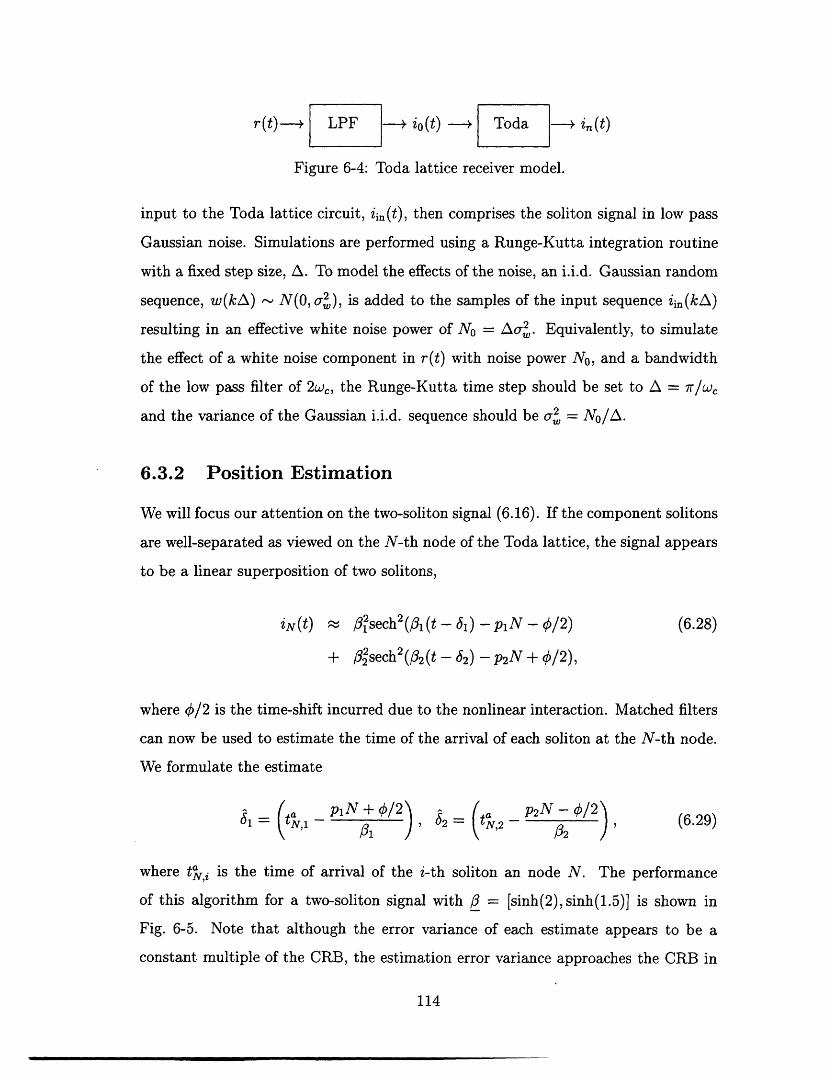
r(t) > LPF - io(t) Toda > in(t)

Figure 6-4: Toda lattice receiver model.

input to the Toda lattice circuit, in(t), then comprises the soliton signal in low pass

Gaussian noise. Simulations are performed using a Runge-Kutta integration routine

with a fixed step size, A. To model the effects of the noise, an i.i.d. Gaussian random

sequence, w(kA) N(O, oa2), is added to the samples of the input sequence iin(kA)

resulting in an effective white noise power of No = Aa2,. Equivalently, to simulate

the effect of a white noise component in r(t) with noise power No, and a bandwidth

of the low pass filter of 2wc, the Runge-Kutta time step should be set to A = r/wc

and the variance of the Gaussian i.i.d. sequence should be cr2 = No/A.

6.3.2 Position Estimation

We will focus our attention on the two-soliton signal (6.16). If the component solitons

are well-separated as viewed on the N-th node of the Toda lattice, the signal appears

to be a linear superposition of two solitons,

iN(t) - 3sech2 (/31(t- 6j) -p 1 N - b/2) (6.28)

+ 0sech2 (6 2 (t - 52) - p 2N + 0/2),

where 0/2 is the time-shift incurred due to the nonlinear interaction. Matched filters

can now be used to estimate the time of the arrival of each soliton at the N-th node.

We formulate the estimate

1 a pNl + - /2) 62 t a p 2 N- /2 (6.29)Si N, 1~~~~~~~ '-- ol2 N,2 - 2-629

where ti is the time of arrival of the i-th soliton an node N. The performance

of this algorithm for a two-soliton signal with / = [sinh(2),sinh(1.5)] is shown in

Fig. 6-5. Note that although the error variance of each estimate appears to be a

constant multiple of the CRB, the estimation error variance approaches the CRB in

114

Il

1

0

0

C

0a).-1

1

.1

' "10- 10-2 10-1 10°noise power, No

Figure 6-5: The CRBs for 61 and 62 are shown with solid and dashed lines, whilethe estimation error results of 100 Monte-Carlo trials are indicated with 'o' and 'x'marks, respectively.

an absolute sense as No -- 0.

6.3.3 Velocity Estimation

Since the velocity of a soliton in the Toda lattice is related to the scale parameter, ,

and the velocity can be estimated based on the arrival times of the soliton, we may

also form an estimate of through velocity estimation. From the set of arrival times,

tNi we have a set of equations for each of the unknown parameters, /3i,

piN + 0/2 = Oltl,N, p2N - /2 = 32tN, (6.30)

which are nonlinear in the parameter i, since Pi = sinh-'(Oi). Solving for the

parameter Pi, we obtain,sinh(pi) 1 (6.31)

Pi ti,N

where tN are the time-difference of arrivals of the i-th soliton between nodes N and

N + 1. Equation (6.31) can be solved numerically using Newton's method and for

115

,0

large p, the solution can also be expressed in terms of Lambert's omega function, Pi =

-Q(-t4N) [9]. We may then formulate the estimate fi = sinh(pi). This technique is

similar to "velocity-filtering" commonly used in seismic signal processing [55]. Note

that in estimating pi, the arrival times ta must be selected based on peak detection

of the signal iN(t) alone without the aid of the matched filter which would require

knowledge of the unknown parameter /3i.

A scalar closed-form sufficient statistic for the estimation of 3 based on observa-

tions of a single soliton in Gaussian noise does not exist due to the highly nonlinear

manner in which the parameter appears both in the time and the amplitude scales of

the signal which preclude factorization of the likelihood function for r(t). Although

an ML solution could be found by numerical maximization of the likelihood function,

such a solution would be computationally intensive. We therefore look at the perfor-

mance of the ad-hoc estimate based on the most salient characteristics of the soliton

through the lattice, namely the scale-dependent velocity.

The results of 100 Monte Carlo trials for the velocity-based estimation algorithm

using a Toda lattice with N = 10 nodes are shown in Fig. 6-6. The parameter values

estimated were 1 sinh(2) and /32 = sinh(1.5) with both solitons time-aligned.

Therefore the CRB for the smaller soliton is actually lower than that for the larger

soliton.

6.3.4 Estimation Based on Inverse Scattering

Although an ML estimate of the parameter /3 cannot be formulated directly based

on observations of the received signal r(t), we can use the inverse scattering frame-

work along with some of the results from Chapter 5 to demonstrate a procedure for

constructing the ML estimate in the high SNR limit. We have argued that ML pa-

rameter estimation based on a received multi-soliton signal, r(t), is equivalent to ML

estimation based on the signal as observed on the N-th node in the Toda lattice,

iN(t). We may also consider the transformation

L(t) = T{r(t)}, (6.32)

116

U

0.0Cu

c0

0

noise power, No

Figure 6-6: The estimation error variance for the velocity-based algorithm. The CRBfor 1 and 2 is shown with a solid and dashed line, and the estimation error variancesare indicated by the points labeled 'o' and 'x' respectively.

where L(t) is the symmetric matrix from the inverse scattering transform. This trans-

formation T{.} is also invertible in principle through inverse scattering. Therefore, an

ML estimate based on the signal L(t) must be the same as an ML estimate based on

r(t). We therefore seek to form an estimate of the parameters of the signal r(t) by per-

forming the estimation in the nonlinear spectral domain. This can be accomplished

as shown in Fig. 6-7 where the Toda lattice can be viewed as a nonlinear filterbank

which projects the signal r(t) onto the spectral components of L(t). This use of the

inverse scattering transform is analogous to performing frequency estimation with the

Fourier transform.

From Chapter 2 we saw that if v~(t) evolves according to the Toda lattice,

i3(t) = (e(vn(t)vni(t)) - e-(Vn+(t)-vn(t))) (6.33)

117

coo

r n(t)

r 1

r2

> L(t)rnFn

rn+l

Figure 6-7: Procedure for computing L(t) by processing the signal r(t) with the Todalattice.

then the eigenvalues of the matrix,

L(t) =

·. an_2(t)

an_(t) bn_(t) an-l(t)

an-l (t) bn (t) an (t)

an (t) bn+l(t) an+l(t)

(6.34)

x('Vn(t)-'Vn+l(t))/2adb.=Jt)2Noehtvn)are time-invariant, where, an(t) = e(vn(t+(t))/2 and b = in(t)/2. Note that v(t)

could correspond to the voltages on the double capacitors in the diode ladder circuit.

Further, the eigenvalues of L(t) for which Ail > 1 correspond to soliton solutions,

with ,i = sinh(cosh-l(Ai)) = /A - 1. We also saw in Chapter 5, that the eigenvalues

of L(t) are, to first order, jointly Gaussian and distributed about the true eigenvalues

corresponding to the original multi-soliton signal, s(t). Therefore, estimation of the

parameters i from the eigenvalues of L(t) as described above constitutes a maximum

likelihood approach in the high SNR limit.

The parameter estimation algorithm now amounts to an estimation of the eigenval-

ues of L(t). Note that since L(t) is tridiagonal, very efficient techniques for eigenvalue

118

estimation may be used [21]. The estimate of the parameter fi is then found by the

relation pi A- 1, where IA/I > 1, and the sign of i can be recovered from the

sign of Ai. Clearly if there is a pre-specified number of solitons, k, present in the

signal, then the k largest eigenvalues would be used for the estimation. If the number

k were unknown, then a simultaneous detection and estimation algorithm would be

required.

In order to perform eigenvalue estimation, we must once again deal with the finite

length of the Toda lattice. This can be resolved by either using the periodic Jacoby

matrix L(t) that results from making the periodic assumption aN(t) = a0o(t),

L(t) =

b (t) al (t) 0 ... aN(t)

al (t) b2 (t) a2 (t)

aN-2(t)

aN-2(t) bN-1(t) aN-1 (t)

- aN(t) 0 ... aN-1 (t) bN (t) _

,7 (6.35)

or by simply truncating the matrix. It can be shown that for the periodic Toda

lattice, the eigenvalues of the periodic Jacoby matrix are time-invariant [68]. In

practice, truncating the matrix around the region of support of the solitons has little

effect on the eigenvalues. Note the similarity once again to the frequency estimation

problem, whereby the Fourier transform cannot be computed explicitly, however the

discrete Fourier Transform, (DFT), is often used which makes similar assumptions

about the region of support of the underlying signal.

An example of the joint estimation of the parameters of a two-soliton signal is

shown in Fig. 6-8. The estimation error variance decreases with the noise power

at the same exponential rate as the CRB. The normalized mean estimation error,

(hi -- i)/i for each estimate Oi are shown in Fig. 6-9, indicating that the estimates

are empirically unbiased.

To verify that the performance of the estimation algorithm has the same depen-

dence on the relative separation of solitons as indicated in Sec 6.2, the estimation

119

-1

.)0

ai_

s

.oEu)

-1

noise power, No

Figure 6-8: The estimation error variance for the inverse scattering-based estimatesof i = sinh(2), /32 = sinh(1.5). The bounds for /31 and /32 are indicated with solidand dashed lines respectively. The estimation results for 100 Monte Carlo trials witha diode lattice of N = 10 nodes for /1 and /32 are indicated by the points labeled 'o'and 'x' respectively.

error variance is also indicated in Fig. 6-10 versus the relative separation, . In the

figure, the mean-squared parameter estimation error for each of the parameters i

are shown along with their corresponding CRB. At least empirically, we see that the

fidelity of the parameter estimates are indeed enhanced by their nonlinear interac-

tion, even though this corresponds to a signal with lower energy, and therefore lower

observational SNR.

6.4 Summary

In this chapter, we have explored some of the properties of multi-soliton signals from

the viewpoint of parameter estimation. In fact, some of the rich structure of these

signals is apparent from the behavior of the Cram6r-Rao bounds for estimating their

parameters. In Chap. 4, we observed that the energy in a two-soliton signal is re-

duced when the component solitons are nonlinearly superimposed. In this chapter,

120

X 10- 3

0Cu

c)E

l10 10 10 10noise power, No

Figure 6-9: Normalized mean parameter estimation error for the inverse scattering-based estimation.

we observed that the nonlinear interaction of solitons can also improve the estimation

performance of each. For certain parameter ranges, the coupling enables the larger

soliton components to enhance the estimation performance of the smaller components.

For multi-soliton parameter estimation, we noted that the coupling of component

solitons can make traditional techniques prohibitively complex. However, using the

nonlinear evolution equations as a preprocessor to perform signal separation, we were

able to perform maximum likelihood time-delay estimation and an associated velocity

estimation.

We also demonstrated an algorithm for multi-soliton parameter estimation based

on the inverse scattering transform. In the high SNR limit, the discrete eigenvalues

in the nonlinear spectrum can be used to formulate maximum likelihood estimates

of the scaling parameters for Toda lattice solitons. This approach is analogous to a

filterbank which measures the content of the received signal in the nonlinear spectrum

of the associated linear operator. Parameter estimation based on inverse scattering

techniques also has many direct analogies to estimation based on Fourier methods for

linear systems.

121

X 10

3.

a 2.5CU

CU

2

C

.o 1.5IUE

W1

0.5

A1 -0.8 -0.6 -0.4 -0.2 0 0.2 0.4 0.6 0.8 1

Separation, 6

Figure 6-10: The estimation error variance for estimating 31 = sinh(2), /2 = sinh(1.5)are indicated with the points labeled 'o' and 'x' and the CRBs for each are indicatedwith solid and dashed lines, respectively.

Perhaps there is something to be gained from a more thorough investigation of the

inverse method in looking for a sufficient statistic for soliton parameter estimation.

The lack of a sufficient statistic for estimation of the parameter /3 stems from the

highly nonlinear manner in which the parameter appears both in the time-scale and

the amplitude scale of the signal

sn(t; ) = 3 2 sech2(sinh- 1(/3)n - 3t). (6.36)

An investigation into exploiting the scale-invariance of such signals and the potential

for multi-scale processing of soliton signals also represents an interesting area for

future work.

122

x X 0 x

x x

o x o

o o

o0 00

… I I I I

3.5

I

Chapter 7

Detection of Soliton Signals

7.1 General Approach

The problem of detecting a single soliton or multiple non-overlapping solitons in

AWGN falls within the theory of classical detection. The general approach to such

problems involves first mapping the observation waveform, r(t) onto a convenient

and suitably compact decision space [72]. The detection problem then reduces to

a partitioning of the decision space into decision regions according to a particular

criteria of optimality. Consider the following binary hypothesis problem,

H0 : r(t) = n(t),

H1 r(t) = -v/s(t) + n(t),

where the received waveform comprises the soliton signal vEs(t) in white Gaus-

sian observational noise n(t) under hypothesis 1, or just the observational noise under

the null hypothesis, for later convenience we have normalized s(t) to have unit en-

ergy. The first task, reduction of r(t) into a convenient decision space, is accomplished

through the sufficient statistic,

r = r(t)s(t), (7.1)

123

which can be efficiently computed with a matched filter.

Once the received signal has been transformed into the decision space, we have

the simple binary hypothesis test

Ho : r = n,

H 1 : r=x/E+n,

where under H0 : r N(0, N 0 ), and under H 1 : r - N(v',N 0 ), where No is the

noise power of the white noise process, n(t). The optimal receiver for a variety of

measures, including the Bayes or Neyman-Pearson criteria, involves a likelihood ratio

test, where the likelihood function is given by

A~)=PrIH1 (RIHl)A(r) = ~s RH)(7.2)PrHo(RHo) (7.2)

resulting in the test

41

NofIt. r(t)s(t)dt lE (773)No ~< ln N0'

When the signal r(t) contains a multi-soliton signal where the component solitons

are not resolved, the detection problem becomes more involved. Specifically, consider

a signal comprising a two-soliton solution to the Toda lattice, where we wish to make

one of four decisions,

H 0 : neither soliton is present,

H1 : only soliton one is present,

H 2 : only soliton two is present,

H 12 : both solitons are present.

If the relative positions of the component solitons are known a priori, then the de-

124

tection problem reduces to deciding which among 4 possible signals is present,

H0 r(t) = n(t),

H 1 r(t) = si(t) + n(t),

H2 r (t) = s2 (t) + n(t),

H1 2 r(t) = s12 (t) + n(t),

where s (t), s2 (t), and s12(t) are soliton one, soliton two and the multi-soliton sig-

nals respectively. Once again, this problem can be solved with standard Gaussian

detection theory.

If the relative positions of the solitons are unknown, as would be the case for a

modulated soliton carrier, then the signal sl2(t) will vary significantly as a function

of the relative separation. Similarly, if the signals are to be transmitted over a soliton

channel where different users occupy adjacent soliton wavenumbers, any detection at

the receiver would have to be performed with the possibility of another soliton com-

ponent present at an unknown position. We therefore obtain a composite hypothesis

testing problem, whereby under each hypothesis, we have

Ho r(t) = n(t)

H1 r(t) = sl(t; 61) + n(t),

H 2 r(t) = s2(t; 62) + n(t),

H 12 r(t) = s l2 (t; _) + n(t),

where 6 = [16, 62]T. The general problem of detection with an unknown parameter, 6,

can be handled in a number of ways. For example, if the parameter can be modeled

as random and the distribution for the parameter were known, p(6), along with the

distributions Pr_6,H(RJ, Hi) for each hypothesis, then the Bayes or Neyman-Pearson

criteria can be used to formulate a likelihood ratio test based on the likelihood func-

125

- -*

tions,

A(r) = f d-p6(i)PrIA,H(Rl, Hi) (7.4)dPJ(6)PJJH(RJ6, Hj)

for i j. Unfortunately, even when the distribution for the parameter d is known,

the likelihood ratios given in (7.4) cannot be found in closed form for even the single

soliton detection problem.

Another approach that is commonly used in radar processing [72, 24] applies

when the distribution of a does not vary rapidly over range of possible values while

the likelihood function (7.4) has a sharp peak as a function of 6. In this case, the

major contribution to the integral in the averaged likelihood function (7.4) is due to

the region around the value of 6 for which A(r; 3) is maximum, and therefore this

value of the likelihood function is used as if the maximizing value, ML, were the

actual value. Since this amounts to a generalization of the standard likelihood ratio

test, it is often called a "generalized likelihood ratio test" (GLRT).

If we plan to employ a GLRT for the multi-soliton detection problem, we are again

faced with the need for an ML estimate of the position, ML. A standard approach to

such problems would involve turning the current problem into one with hypotheses

H0 , H1 , and H 2 as before, and an additional M hypotheses - one for each value of the

parameter 6 sampled over a range of possible values. Additionally, the complexity of

the detection problem increases exponentially with the number of component solitons,

N , resulting in a hypothesis testing problem with (M + )N hypotheses.

However, as with the estimation problems in Chap. 6, the detection problems can

be decoupled by preprocessing the signal r(t) with the Toda lattice. If the component

solitons separate as viewed on the N-th node in the lattice, then the detection problem

can be more simply formulated using iN(t). The invertibility of the lattice equations

implies that a Bayes optimal decision based on r(t) must be the same as that based

on iN(t). Since the Bayes optimal decision can be performed based on the likelihood

function A(r(t)), and A(iN(t)) = A(T{r(t)}) = A(r(t)), the optimal decisions based

on r(t) and iN(t) must be the same for any invertible transformation T{.}. Although

we will be using a GLRT, where the value of ML is used for the unknown positions

126

of the multi-soliton signal, since the ML estimates based on r(t) and iN(t) must also

be the same, as shown in Chap. 6, the detection performance of a GLRT using those

estimates must also be the same. Since at high SNR, the noise component of the

signal iN(t) can be assumed low pass and Gaussian, as in Chap. 6, the GLRT can be

performed by pre-processing r(t) with the Toda lattice equations followed by matched

filter processing.

7.2 Simulations

To illustrate the algorithm, we consider the hypothesis test between H 0 and H 12,

where the separation of the two solitons, , - 62, varies randomly in the interval

[-1//32,1/32]. The detection processor comprises a Toda lattice of N = 20 nodes,

with the detection performed based on the signal io(t). To implement the GLRT,

we search over a fixed time interval about the expected arrival time for each soliton.

In this manner we obtain a sequence of 1000 Monte Carlo values of the processor

output for each hypothesis. A set of Monte Carlo runs has been completed for each

of 3 different levels of the noise power, No.

The receiver operating characteristic (ROC) for the soliton with 32 = sinh(1.5) is

shown in Fig. 7-1, where the probability of detection, PD, for this hypothesis test is

shown as a function of the false alarm probability, PF. For comparison, we also show

the ROC that would result from a detection of the soliton alone, at the same noise level

and with the time-of-arrival known. The detection index, d = E/No, is indicated

for each case, where E is the energy in the component soliton. The corresponding

results for the larger soliton are qualitatively similar, although the detection indices

for that soliton alone, with /1 = sinh(2), are 5.6, 4, and 3.3, respectively. Therefore

the detection probabilities are considerably higher for a fixed probability of false

alarm. Note that the detection performance for the smaller soliton is well modeled by

the theoretical performance for detection of the smaller soliton alone. This implies,

at least empirically, that the ability to detect the component solitons in a multi-

soliton signal appears to be unaffected by the nonlinear coupling with other solitons.

127

Further, although the unknown relative separation results in significant waveform

uncertainty and would require a prohibitively complex receiver for standard detection

techniques, Bayes optimal performance can still be achieved with a minimal increase

in complexity.

n

Figure 7-1: A set of empirically generated ROCs are shown for the detection of thesmaller soliton from a two-soliton signal. For each of the three noise levels, the ROCfor detection of the smaller soliton alone is also indicated along with the correspondingdetection index, d.

7.3 Summary and Further Considerations

In this chapter we address the problem of multi-soliton detection in an AWGN envi-

ronment. Our approach is to exploit the soliton evolution equations as a preproces-

sor, separating the multi-soliton observation into component solitons. Focusing on

the Toda lattice as an example, at high signal-to-noise ratios, the noise component

in the receiver remains low pass and Gaussian and is decoupled from the solitons.

This allows each of the component solitons to be detected with standard matched

filter processing using a GLRT. Empirically generated ROCs seem to indicate that

128

13=sinh(1.5)

PF ~1

the detection performance for the component solitons is comparable to that for single

soliton observations.

One outstanding issue is the determination of appropriate bounds on the theoret-

ical performance of the GLRT for the detection of soliton and multi-soliton signals.

Both when the Toda lattice is used for signal separation of a multi-soliton signal and

when a single soliton is observed with unknown arrival time, the probability of detec-

tion and the false alarm rate have to be computed empirically, due to the complexity

of the required calculations. The false alarm rate of a GLRT for a single soliton

detection with unknown arrival time is determined by the level crossing problem,

whereby we seek the probability that the output of the matched filter will cross a

given threshold over a fixed time interval. A description of this problem is given in

[24]. In general, determination of the false alarm rate is difficult, however there are a

few well-studied cases. For example, based on Siegert's work with Markov processes,

Helstrom shows that for a first order Gauss-Markov process with auto-covariance,

Rx(r) = R(O)e - l I , for large time intervals, aT > 1, the probability of false alarm

is given approximately by [24]

-T a?7 ~22R)Pfa 1 - e - , v = e- 2/2R(O) (7.5)

2~irR(O)

where it is assumed that the threshold, / > R(O). When a matched filter is used for

detecting a single soliton of unknown arrival time, our matched filter can be roughly

approximated by a filter with impulse response, h(t) = 2 e -2 6l1r. The corresponding

matched filter output for a white noise input will have auto-covariance of the form

f4(2 + lTIl)e - 2 1T and for > 1 will behave much like a first order Gauss Markov

process. In this manner, we might obtain a better estimate of the expected false alarm

rate for single and multi-soliton detection with unknown position. For modest signal

to noise ratios, the detection probability is well-modeled by the detection probability

of a processor with the arrival time known.

129

130

Chapter 8

Conclusions and Directions for

Future Work

In this thesis, we have developed a framework for exploring the generation and pro-

cessing of soliton signals and introduced some potentially important applications of

solitons in the broad context of communications.

We have taken the viewpoint of using solitons as carrier signals for transmission

over linear, rather than nonlinear channels. The nonlinear evolution equations can

then be viewed as specialized processors of this class of signals, which are naturally

suited to performing a number of complex signal processing tasks. For example,

these systems can efficiently generate soliton signals and can perform the nonlinear

signal separation of multi-soliton carriers necessary for multiplexing and demultiplex-

ing multiple users in a potential soliton wireless communications context.

Focusing specifically on two soliton systems, the Toda lattice and the discrete-

KdV equation, we develop new electrical analogs for the generation and processing of

soliton signals. Although analog circuit models have been previously developed for a

variety of nonlinear wave equations in general, and for the Toda lattice in particular,

our diode ladder implementation is the first direct electrical analog of this soliton

system. Further, this appears to be the first circuit model of the Toda lattice which is

sufficiently accurate to demonstrate true soliton interactions. The diode ladder circuit

was implemented in hardware using standard components and provides a platform for

131

the further development and testing of real-time soliton processing techniques. We

have also developed a new circuit model for the discrete-KdV equation; a nonlinear

system which was largely ignored for having no prior electrical or mechanical analog.

The discrete-KdV circuit provides a framework for processing discrete-time soliton

signals.

Based on these nonlinear circuit models, we have suggested and explored a number

of communications techniques whereby message-bearing signals are used to modulate

the parameters of soliton carriers. The nonlinear circuits are used to generate and

to multiplex multiple message-signals onto a multi-soliton carrier. We have demon-

strated that the nonlinear interaction of multiple solitons can be exploited as a means

of reducing the transmitted signal energy in a multi-user communication context.

To assess the efficacy and the robustness of these communication techniques in

the presence of background noise, we have analyzed the effects of small amplitude

disturbances on the processing of soliton signals in the Toda lattice and characterized

the statistics of the noise as it is processed. We have shown that in a high SNR AWGN

background, the dynamics of soliton signals are practically unperturbed. Also, the

noise component of the received signal remains essentially low pass and Gaussian.

Through an analysis of the nonlinear spectrum from the inverse scattering transform,

we also have shown that at high SNR, virtually all of the background noise maps onto

the non-soliton (continuum) component of the nonlinear spectrum, and the soliton

spectrum experiences only a small Gaussian perturbation. This result furthers the

analogy of the inverse scattering transform to the Fourier transform for linear systems.

We were also able to develop maximum likelihood parameter estimation algorithms

for soliton signals corrupted by white Gaussian noise. Calculation of the Cramer-Rao

bounds for the estimation error variance of soliton parameters reveals the potential for

estimation enhancement due to multiple soliton interaction. By using the nonlinear

circuits as preprocessors which perform the necessary signal separation, the joint

estimation of multiple soliton parameters can be achieved through standard Gaussian

techniques. We have also developed a maximum likelihood parameter estimation

algorithm in the nonlinear spectral domain of the inverse scattering transform. Both

132

the theoretical bounds and the empirical algorithm performance demonstrate that

the nonlinear coupling of multiple solitons can actually enhance parameter estimation

performance. This indicates the potential for wireless multi-soliton communication

techniques to simultaneously reduce the transmitted signal energy while enhancing

communication performance.

By a similar technique, soliton circuits can be used to decompose a multi-soliton

detection problem with (M + )Ns hypotheses into Ns-separate binary hypothesis

tests without sacrificing Bayes optimality in high SNR Gaussian environments. Of

particular interest is the case of multi-soliton position uncertainty which can gives rise

to dramatic changes in the received multi-soliton signal and therefore would have a

significant impact on the structure of a traditional detector. However, since the soliton

circuits decompose the multi-soliton detection problem into single soliton detections,

our detection framework is unchanged.

8.1 Future Directions

In this thesis, we began an exploration of a number of new and interesting applications

of soliton signals and systems from a signal processing viewpoint. As a result, there

are a number outstanding issues relating to many of the topics considered. Although

many areas of future study have been identified in the body of the thesis, we mention

several particularly intriguing directions here.

Much of the mathematical foundation for soliton dynamics lies within the frame-

work of solvable nonlinear systems. In Sec. 2.2 we have attempted to present some

of the essential ideas behind this class of nonlinear systems and relate them to linear

system theory. Although many of the results in this thesis pertain to the detection

and estimation of parameters of received soliton signals, there are many interesting

signal processing questions regarding the dynamics these integrable nonlinear systems

themselves. Specifically, it may be possible to address the problems of recursive esti-

mation, e.g., prediction, extrapolation, filtering, and smoothing of such systems with

the aid of the inverse scattering. Traditional barriers to such investigations for nonlin-

133

ear systems lie in both the state propagation and the propagation of state probability

densities. For integrable Hamiltonian systems, the state propagation can be solved

explicitly via inverse scattering, while the propagation of the state density remains a

difficult problem.

Another potentially interesting area of future research involves extending the re-

sults of integrable system theory to include totally discrete (discrete-time, finite di-

mensional) systems. Some work in this area has led to discretized versions of the

inverse scattering theory for the Toda lattice [20, 26, 28] the Korteweg-de Vries

equation[25], as well as others in [1, 27]. Such systems may lead to applications

using discrete soliton signals for digital communication.

In Chap. 3 we illustrate how analog circuits could be used in the context of the

communication ideas shown in Chap. 4. These results along with those of Hirota and

Suzuki [29, 64, 65], Toda [68], Scott [56, 57], and others illustrate the potential for

development of a variety of analog hardware for soliton modulation techniques. How-

ever, there are several outstanding issues regarding the detailed implementation of

the communications techniques discussed in Chap. 4 using such circuits. Specifically,

the demodulation of individual soliton carriers still must be addressed along with a

more complete investigation into the effects of realistic non-additive channel distur-

bances. There may also be benefit to further exploration of the soliton-like behavior

of certain cellular automata [1, 7, 53, 66] and the possible use of such systems for

digital communication or computation [32, 62, 63].

The nonlinear circuit models developed for the Toda lattice demonstrate an in-

teresting similarity to the models used by Keshner in his analysis of 1/f noise [38].

Specifically, a small signal model for the diode ladder circuit yields a driving point

impedance inversely proportional to frequency, and thus would produce a "double

Brownian" motion process in response to a white noise input. Such an analogy leads

directly to the observation that at least for the small signal model, noise at the in-

put of the nonlinear circuits will lead to 1/f-type disturbances. Another interesting

link between the 1/f generators and soliton circuits, is that, like the family of 1/f

random processes, the family of soliton solutions to such equations also have a multi-

134

scale component. This apparent multi-scale invariance of the soliton dynamics along

with the similarity in the circuit models to those which generate 1/f noise, may in-

dicate the presence of a fundamental nonlinear multi-scale behavior inherent in the

dynamics.

Although we have explored some basic strategies for using soliton signals for com-

munication, there remain a number of unanswered questions regarding the efficacy

of such techniques in comparison to standard methods. For example, a quantitative

investigation of the spectral efficiency, the effects of inter-symbol interference, the

error probability, or decoder complexity for such methods in comparison to standard

techniques ought to be undertaken. Finally, we note that solitons represent a rich

class of signals that are potentially applicable to a variety of signal processing and

communications contexts beyond those mentioned in this thesis. Indeed, perhaps

the most exciting and potentially rewarding direction for future research lies in the

discovery of new and promising applications.

135

136

Bibliography

[1] M.J. Ablowitz and A.P. Clarkson. Solitons, Nonlinear Evolution Equations andInverse Scattering. Number 149 in London Mathematical Society Lecture NoteSeries. Cambridge University Press, Cambridge, Great Britain, 1991.

[2] M. Abramowitz and I.A. Stegun, editors. Handbook of Mathematical Functions.Dover, New York, NY, 1965.

[3] V.I. Arnold and A. Avez. Ergodic Problems of Classical Mechanics. Addison-Wesley Publishing Company, Inc., 1989.

[4] G.J. Ballantyne, P.T. Gough, and D.P. Taylor. Periodic solutions of Toda latticein loop nonlinear transmission line. Electronics Letters, 29(7):607-609, April1993.

[5] T.B. Benjamin. The stability of solitary waves. Proceedings of the Royal Societyof London, A(328):1553-183, 1972.

[6] Rajendra Bhatia. Perturbation bounds for matrix eigenvalues. Pitman researchnotes in mathematics series. Wiley, 1987.

[7] Alexander Bobenko, Martin Bordermann, Charlie Gunn, and Ulrich Pinkall. Ontwo integrable cellular automata. Communications in Mathematical Physics,158:127-134, 1993.

[8] Rene Carmona. Spectral theory of random Schrddinger operators. Birkhauser,1990.

[9] B. Char, K. Geddes, G. Gonnet, B. Leong, M. Monagan, and S. Watt. Maple VLibrary Reference Manual. Springer-Verlag, 1992.

[10] Yasuo Cho, Junji Wakita, and Nozomu Miyagawa. Nonlinear equivalent circuitmodel analysis of acoustic devices and propagation of surface acoustic wave.Japan Journal of Applied Physics, 32(5B):2261-2264, 1993.

[11] Proceedings of the IEEE: Special issue on surface acoustic wave devices andapplications. L.T. Claiborne, G.S. Kino and E. Stern, editors, May 1976.

[12] P.G. Drazin and R.S. Johnson. Solitons: an Introduction. Cambridge Texts inApplied Mathematics. Cambridge University Press, New York, 1989.

137

[13] A. Erdelyi, editor. Tables of Integral Transforms, volume I. McGraw-Hill BookCompany, 1954. Based, in part, on notes left by Harry Bateman, and compiledby The Bateman Manuscript Project.

[14] E. Fermi, J.R Pasta, and S.M Ulam. Studies of nonlinear problems. In CollectedPapers of E. Fermi, volume II, pages 977-988. University of Chicago Press, 1965.

[15] H. Flaschka. On the Toda lattice. ii. Progress of Theoretical Physics, 51(3):703-716, March 1974.

[16] H. Flaschka and D.W. McLaughlin. Some comments on B/cklund transforma-tions, canonical transformations, and the inverse scattering method. In RobertMiura, editor, Backlund transformations, the inverse scattering method, solitons,and their applications: Proceedings NSF Research Workshop on Contact Trans-formations, number 515 in Lecture notes in mathematics, pages 253-295, Berlin,1976. Springer-Verlag.

[17] Nikos Flytzanis, Boris Malomed, and Jonathan A.D. Wattis. Analysis of stabilityof solitons in one-dimensional lattices. Physics Letters, A(180):107-112, 1993.

[18] Clifford S. Gardner, John M. Greene, Martin D. Kruskal, and Robert Miura.Method for solving the Korteweg-deVries equation. Physical Review Letters,19(19):1095-1097, November 1967.

[19] A. Gelb, editor. Applied Optimal Estimation. MIT Press, Cambridge, MA, 1974.

[20] John Gibbons and Boris Kupershmidt. Time discretizations of lattice integrablesystems. Physics Letters, A(165):105-110, May 1992.

[21] Gene H. Golub and Charles F. Van Loan. Matrix Computations. The JohnsHopkins University Press, Baltimore, Maryland, 1989.

[22] I.S. Gradshteyn and I.M. Ryzhik. Table of Integrals, Series and Products. Aca-demic Press, fourth edition, 1965.

[23] Hermann A. Haus. Molding light into solitons. IEEE Spectrum, pages 48-53,March 1993.

[24] Carl W. Helstrom. Statistical Theory of Signal Detection. Pergamon Press, NewYork, second edition, 1968.

[25] Ryogo Hirota. Nonlinear partial difference equations. I. a difference analogueof the Korteweg-de Vries equation. Journal of the Physical Society of Japan,43(4):1424-1433, October 1977.

[26] Ryogo Hirota. Nonlinear partial difference equations. II. discrete-time Todaequation. Journal of the Physical Society of Japan, 43(6):2074-2078, December1977.

138

[271 Ryogo Hirota. Nonlinear partial difference equations. III. discrete sine-Gordonequation. Journal of the Physical Society of Japan, 43(6):2079-2087, December1977.

[28] Ryogo Hirota. Nonlinear partial difference equations. IV. Bicklund transfor-mation for the discrete-time Toda equation. Journal of the Physical Society ofJapan, 45(1):321-332, July 1978.

[29] Ryogo Hirota and Kimio Suzuki. Theoretical and experimental studies of latticesolitons in nonlinear lumped networks. Proc. IEEE, 61(10):1483-1491, October1973.

[30] Paul Horowitz and Winfield Hill. The Art of Electronics. Cambridge UniversityPress, New York, second edition, 1989.

[31] Eryk Infeld and George Rowlands. Nonlinear Waves, Solitons and Chaos. Cam-bridge University Press, New York, 1990.

[32] Nayeem Islam, J.P. Singh, and Kenneth Steiglitz. Soliton phase shifts in a dis-sipative lattice. J. Appl. Phys., 62(2):689-693, July 1987.

[33] M. Kac and P. van Moerbeke. On an explicitly soluble system of nonlineardifferential equations related to certain Toda lattices. Advances in Mathematics,16:160-169, 1975.

[34] M. Kac and P. van Moerbeke. On some periodic Toda lattices. Proc. Nat. Acad.Sci., 72(4):1627-1629, April 1975.

[35] J.F. Kaiser. On a simple algorithm to calculate the 'energy' of a signal. In Proc.Int. Conf. Acoust. Speech, Signal Processing, pages 381-384, Albuquerque, NM,1990.

[36] J.F. Kaiser. personal communication, June 1994.

[37] Tosio Kato. Perturbation theory for linear operators. Springer-Verlag, 1980.

[38] M.S. Keshner. 1f noise. Proc. IEEE, 70:212-218, March 1982.

[39] Joseph A Kolosick, Don L Landt, H.C. Hsuan, and Karle E. Lonngren. Propertiesof solitary waves as observed on a nonlinear dispersive transmission line. Proc.IEEE, 62(5):578-581, May 1974.

[40] Yinchieh Lai. Noise analysis of soliton communication systems-a new approach.Journal of Lightwave Technology, 11(3):462-467, March 1993.

[41] L.D. Landau and E.M. Lifshitz. Mechanics. Pergamon Press, New York, 1976.

[42] Peter D. Lax. Integrals of nonlinear equations of evolution and solitary waves.Communications on Pure and Applied Mathematics, XXI:467-490, 1968.

139

[43] A.G. Lindgren and R.J. Buratti. Stability of waveforms on active nonlineartransmission lines. IEEE transactions on Circuit Theory, CT-16:274-279, Aug1969.

[44] V.M. Loginov. Exact separation of an additive mixture of a determinate sig-nal and gaussian noise by the use of Korteweg-de Vries solitons. Tech. Phys.Lett.(Pis'ma Zh. Tekh. Fiz.), 19(7):433-434, July 1993.

[45] S.V. Manakov. Complete integrability and stochastization of discrete dynamicalsystems. Soy. Phys. JETP, 40(2):269-274, 1975.

[46] N. Margolus and T. Toffoli. Cellular automata machines. In G.D. Doolen, editor,Lattice Gas Methods for Partial Differential Equations, pages 219-249, Reading,Ma, 1990. Addison-Wesley.

[47] Meta Software, Inc., Campbell, CA. HSPICE User's Manual, 1992.

[48] J. Moser. Finitely many mass points on the line under the influence of an expo-nential potential - an integrable system. In J. Moser, editor, Dynamical Systems,Theory and Applications: Battelle Seattle 1974 Rencontres, number 38 in LectureNotes in Physics, pages 467-497, New York, 1975. Springer Verlag.

[49] Alan C. Newell. Solitons in Mathematics and Physics. Regional ConferenceSeries in Applied Mathematics. Society for Industrial and Applied Mathematics,Philadelphia, 1985.

[50] Yoshiko Okada, Shinsuke Watanabe, and Hiroshi Tanaca. Solitary wave in peri-odic nonlinear lattice. Journal of the Physical Society of Japan, 59(8):2647-2658,August 1990.

[51] Naotake Ooyama and Nobuhiko Saito. On the stability of lattice solitons. Sup-plement of the Progress of Theoretical Physics, 45:201-208, 1970.

[52] T.S. Papatheodorou, M.J. Ablowitz, and Y.G. Saridakis. A rule for fast com-putation and analysis of soliton automata. Studies in Applied Mathematics,79:173-184, 1988.

[53] James K. Park, Kenneth Steiglitz, and William P. Thurston. Soliton-like behav-ior in automata. Physica 19D, pages 423-432, 1986.

[54] V.N. Popov, editor. Operator theory with a random potential, and some questionsof statistical physics: collection of papers. American Mathematical Society, 1991.

[55] Enders A. Robinson and Sven Treitel. Geophysical Signal Analysis. Prentice-Hall,Inc., 1980.

[56] A.C. Scott. Active and Nonlinear Wave Propagation in Electronics. Wiley-Interscience, New York, 1970.

140

[57] Alwyn C. Scott, F.Y.F. Chu, and David McLaughlin. The soliton: A new conceptin applied science. Proc. IEEE, 61(10):1443-1483, October 1973.

[58] John Scott-Russell. Report on waves. In Rep. 14th Meet. Brit. Assoc. Adv. Sci.,pages 319-320, 1844.

[59] William McC. Siebert. Circuits, Signals, and Systems. The MIT ElectricalEngineering and Computer Science Series. The MIT Press and The McGraw-Hill Book Company, Cambridge MA, 1986.

[60] Andrew C. Singer. A new circuit for communication using solitons. In Proc.IEEE Workshop on Nonlinear Signal and Image Processing, volume I, pages150-153, 1995.

[61] Merrill I. Skolnik. Radar Handbook. McGraw-Hill Book Company, 1970.

[62] Richard K. Squire and Ken Steiglitz. Subatomic particle machines: parallelprocessing in bulk material. submitted to IEEE Signal Processing Letters, 1995.

[63] Kenneth Steiglitz, Irfan Kamal, and Arthur Watson. Embedding computationin one-dimensional automata by phase coding solitons. IEEE Transactions onComputers, 37(2):138-145, February 1988.

[64] Kimio Suzuki, Ryogo Hirota, and Kazufumi Yoshikawa. Amplitude modulatedsoliton trains and coding-decoding applications. Int. J. Electronics, 34(6):777-784, 1973.

[65] Kimio Suzuki, Ryogo Hirota, and Kazufumi Yoshikawa. The properties of phasemodulated soliton trains. Japanese Journal of Applied Physics, 12(3):361-365,March 1973.

[66] D. Takahashi. On a fully discrete soliton system. In M. Boiti, L. Martina, andF. Pempinelli, editors, Nonlinear Evolution Equations and Dynamical Systems,pages 245-249, New Jersey, June 1991. World Scientific.

[67] Morikazu Toda. Theory of Nonlinear Lattices. Number 20 in Springer Series inSolid-State Science. Springer-Verlag, New York, 1981.

[68] Morikazu Toda. Nonlinear lattice and soliton theory. IEEE Transactions onCircuits and Systems, CAS-30(8):542-554, August 1983.

[69] Morikazu Toda. Nonlinear Waves and Solitons. Mathematics and Its Applica-tions. Klewer Academic Publishers, Boston, 1989.

[70] T. Toffoli and N. Margolus. Cellular Automata Machines - A New Environmentfor Modeling. MIT Press, Cambridge, Ma, 1987.

[71] T. Toffoli and N. Margolus. Programmable matter: Concepts and realizations.Physica D, 47(1-2):263-272, 1991.

141

[72] Harry L. Van Trees. Detection, Estimation, and Modulation Theory: Part IDetection, Estimation and Linear Modulation Theory. John Wiley and Sons,1968.

[73] J. vomScheidt and W. Purkert. Random Eigenvalue Problems. Probability andApplied Mathematics. North Holland, 1983.

[74] Miki Wadati. Stochastic Korteweg-de Vries equation. Journal of the PhysicalSociety of Japan, 52(8):2642-2648, Aug 1983.

[75] G.B. Whitham. Linear and Nonlinear Waves. Wiley, New York, 1974.

[76] J.H. Wilkinson. The algebraic eigenvalue problem. Oxford science publications.Oxford University Press, 1988.

[77] G.W. Wornell and A.V. Oppenheim. Wavelet-based representations for a class ofself-similar signals with application to fractal modulation. IEEE Trans. Inform.Theory, 38(2):785-800, March 1992.

[78] N.J. Zabusky and M.D. Kruskal. Interaction of solitons in a collisionless plasmaand the recurrence of initial states. Physical Review Letters, 15(6):240-243, Au-gust 1965.

[79] V.E. Zakharov and A.B. Shabat. A refined theory of two-dimensional self-focussing and one-dimensional self-modulation of waves in nonlinear media. Zh.Eksp. Teor. Fiz., 61(1):118-134, 1971.

142