NBER WORKING PAPER SERIES

SIMPLE AND ROBUST RULES FOR MONETARY POLICY

John B. TaylorJohn C. Williams

Working Paper 15908http://www.nber.org/papers/w15908

NATIONAL BUREAU OF ECONOMIC RESEARCH1050 Massachusetts Avenue

Cambridge, MA 02138April 2010

We thank Andy Levin, Mike Woodford, and other participants at the Handbook of Monetary EconomicsConference for helpful comments and suggestions. We also thank Justin Weidner for excellent researchassistance. The opinions expressed are those of the authors and do not necessarily reflect the viewsof the management of the Federal Reserve Bank of San Francisco, the Board of Governors of the FederalReserve System, or the National Bureau of Economic Research.

NBER working papers are circulated for discussion and comment purposes. They have not been peer-reviewed or been subject to the review by the NBER Board of Directors that accompanies officialNBER publications.

© 2010 by John B. Taylor and John C. Williams. All rights reserved. Short sections of text, not toexceed two paragraphs, may be quoted without explicit permission provided that full credit, including© notice, is given to the source.

Simple and Robust Rules for Monetary PolicyJohn B. Taylor and John C. WilliamsNBER Working Paper No. 15908April 2010JEL No. E5

ABSTRACT

This paper focuses on simple rules for monetary policy which central banks have used in various waysto guide their interest rate decisions. Such rules, which can be evaluated using simulation and optimizationtechniques, were first derived from research on empirical monetary models with rational expectationsand sticky prices built in the 1970s and 1980s. During the past two decades substantial progress hasbeen made in establishing that such rules are robust. They perform well with a variety of newer andmore rigorous models and policy evaluation methods. Simple rules are also frequently more robustthan fully optimal rules. Important progress has also been made in understanding how to adjust simplerules to deal with measurement error and expectations. Moreover, historical experience has shownthat simple rules can work well in the real world in that macroeconomic performance has been betterwhen central bank decisions were described by such rules. The recent financial crisis has not changedthese conclusions, but it has stimulated important research on how policy rules should deal with assetbubbles and the zero bound on interest rates. Going forward the crisis has drawn attention to the importanceof research on international monetary issues and on the implications of discretionary deviations frompolicy rules.

John B. TaylorHerbert Hoover Memorial BuildingStanford UniversityStanford, CA 94305-6010and NBERJohn.Taylor@stanford.edu

John C. WilliamsFederal Reserve Bank of San FranciscoEconomic Research Department, MS 1130101 Market St.San Francisco, CA 94105john.c.williams@sf.frb.org

2  

Economists have been interested in monetary policy rules since the advent of economics.

In this review paper we concentrate on more recent developments, but we begin with a brief

historical summary to motivate the theme and purpose of our paper. We then describe the

development of the modern approach to policy rules and evaluate the approach using experiences

before, during, and after the Great Moderation. We then contrast in detail this policy rule

approach with optimal control methods and discretion. Finally we go on to consider several key

policy issues, including the zero bound on interest rates and issue of bursting bubbles, using the

lens of policy rules.

1. Historical Background

Adam Smith first delved into the subject monetary policy rules in the Wealth of Nations

arguing that “a well-regulated paper-money” could have significant advantages in improving

economic growth and stability compared to a pure commodity standard. By the start of the 19th

century Henry Thornton and then David Ricardo were stressing the importance of rule-guided

monetary policy after they saw the monetary-induced financial crises related to the Napoleonic

Wars. Early in the 20th century Irving Fisher and Knut Wicksell were again proposing monetary

policy rules to avoid monetary excesses of the kinds that led to hyperinflation following World

War I or seemed to be causing the Great Depression. And later, after studying the severe

monetary mistakes of the Great Depression, Milton Friedman proposed his constant growth rate

rule with the aim of avoiding a repeat of those mistakes. Finally, modern-day policy rules, such

as the Taylor (1993a) Rule, were aimed at ending the severe price and output instability during

the Great Inflation of the late 1960s and 1970s (see also Asso, Kahn, and Leeson, 2007, for a

detailed review).

3  

As the history of economic thought makes clear, a common purpose of these reform

proposals was a simple, stable monetary policy that would both avoid creating monetary shocks

and cushion the economy from other disturbances, and thereby reduce the chances of recession,

depression, crisis, deflation, inflation, and hyperinflation. There was a presumption in this work

that some such simple rule could improve policy by avoiding monetary excesses, whether related

to money finance of deficits, commodity discoveries, gold outflows, or mistakes by central

bankers with too many objectives. In this context, the choice between a monetary standard

where the money supply jumped around randomly versus a simple policy rule with a smoothly

growing money and credit seemed obvious. The choice was both broader and simpler than

“rules versus discretion.” It was “rules versus chaotic monetary policy” whether the chaos was

caused by discretion or unpredictable exogenous events like gold discoveries or shortages.

A significant change in economists’ search for simple monetary policy rules occurred in

the 1970s, however, as a new type of macroeconomic model appeared on the scene. The new

models were dynamic, stochastic, and empirically estimated. But more important, these

empirical models incorporated both rational expectations and sticky prices, and they therefore

were sophisticated enough to serve as a laboratory to examine how monetary policy rules would

work in practice. These were the models that were used to find new policy rules, such as the

Taylor Rule, to compare the new rules with earlier constant growth rate rules or with actual

policy, and to check the rules for robustness. Examples of empirical modes with rational

expectations and sticky prices include the simple three equation econometric model of the United

States in Taylor (1979), the multi-equation international models in the comparative studies by

Bryant, Hooper, and Mann (1993), and the econometric models in robustness analyses of Levin,

Wieland, and Williams (1999). More or less simultaneously, practical experience was

4  

confirming the model simulation results as the instability of the Great Inflation of the 1970s gave

way to the Great Moderation around the same time that actual monetary policy began to

resemble the simple policy rules that were proposed.

While the new rational expectations models with sticky prices further supported the use

of policy rules—in keeping with the Lucas (1976) critique and time inconsistency (Kydland and

Prescott, 1977)—there was no fundamental reason why the same models could not be used to

study more complex discretionary monetary policy actions which went well beyond simple rules

and used optimal control theory. Indeed, before long optimal control theory was being applied to

the new models, refined with specific micro-foundations as in Rotemberg and Woodford (1997),

Woodford (2003), and others. The result was complex paths for the instruments of policy which

had the appearances of “fine tuning” as distinct from simple policy rules.

The idea that optimal policy conducted in real time without the constraint of simple rules

could do better than simple rules thus emerged within the context of the modern modeling

approach. The papers by Mishkin (2007) and Walsh (2009) at recent Jackson Hole Conferences

are illustrative. Mishkin (2007) uses optimal control to compute paths for the federal funds rate

and contrasts the results with simple policy rules, stating that in the optimal discretionary policy

“the federal funds rate is lowered more aggressively and substantially faster than with the

Taylor-rule….This difference is exactly what we would expect because the monetary authority

would not wait to react until output had already fallen.” The implicit recommendation of this

statement is that simple policy rules are inadequate for real world policy situations and that

policymakers should therefore deviate from them as needed.

The differences in these approaches are profound and have important policy implications.

At the same Jackson Hole conference that Mishkin (2007) emphasized the advantages of

5  

deviating from policy rules, Taylor (2007) showed that one such deviation added fuel to the

housing boom and thereby helped bring on the severe financial crisis, the deep recession, and

perhaps the end of the Great Moderation. For these reasons we focus on the differences between

these two approaches in this paper. Like all previous studies of monetary policy rules by

economists, our goal is to find ways to avoid such economic maladies.

We start in the next section with a review of the development of optimal simple monetary

policy rules using quantitative models. We then consider the robustness of policy rules using

comparative model simulations and show that simple rules are more robust than fully optimal

rules. The most recent paper in the Elsevier Handbook in Economics series on monetary policy

rules is the comprehensive and widely-cited survey published by Ben McCallum (1999) in the

Handbook of Macroeconomics (Taylor and Woodford, 1999). Our paper and McCallum’s are

similar in scope in that they focus on policy rules which have been designed for normative

purposes rather than on policy reaction functions which have been estimated for positive or

descriptive purposes. In other words, the rules we study have been derived from economic

theory or models and are designed to deliver good economic performance, rather than to fit

statistically the decisions of central banks. Of course, such normative policy rules can also be

descriptive if central bank decisions follow the recommendations of the rules which they have in

many cases. Research of an explicitly descriptive nature, which focuses more on estimating

reaction functions for central banks, goes back to Dewald and Johnson (1963), Fair (1978), and

McNees (1986), and includes, more recently, work by Meyer (2009) on estimating policy rules

for the Federal Reserve.

McCallum’s Handbook of Macroeconomics paper stressed the importance of robustness

of policy rules and explored the distinction between rules and discretion using the time

6  

inconsistency principles. His survey also clarified important theoretical issues such as uniqueness

and determinacy and he reviewed research on alternative targets and instruments, including both

money supply and interest rate instruments. Like McCallum we focus on the robustness of

policy rules. We focus on policy rules where the interest rate rather than the money supply is the

policy instrument, and we place more emphasis on the historical performance of policy rules

reflecting the experience of the dozen years since McCallum wrote. We also examine issues that

have been major topics of research in academic and policy circles since then, including policy

inertia, learning, and measurement errors. We also delve into the issues that arose in the recent

financial crisis including the zero lower bound on interest rates and dealing with asset price

bubbles. In this sense, our paper is complementary to McCallum’s useful Handbook of

Macroeconomics paper on monetary policy rules.

2. Using Models to Evaluate Simple Policy Rules

The starting point for our review of monetary policy rules is the research that began in the

mid 1970s, took off in the 1980s and 1990s, and is still expanding. As mentioned above, this

research is conceptually different from previous work by economists in that it is based on

quantitative macroeconomic models with rational expectations and frictions/rigidities, usually in

wage and price setting.

We focus on the research based on such models because it seems to have led to an

explosion of practical as well as academic interest in policy rules. As evidence consider, Don

Patinkin’s (1956) Money, Interest, and Prices, which was the textbook in monetary theory in

many graduate school in the early 1970s. It has very few references to monetary policy rules. In

contrast, the modern day equivalent, Michael Woodford’s (2003) book, Interest and Prices, is

7  

packed with discussions about monetary policy rules. In the meantime, thousands of papers have

been written on monetary policy rules since the mid 1970s. The staffs of central banks around

the world regularly use policy rules in their research and policy evaluation (see for example,

Orphanides, 2008) as do practitioners in the financial markets.

Such models were originally designed to answer questions about policy rules. The

rational expectations assumption brought attention to the importance of consistency over time

and to predictability, whether about inflation or policy rule responses, and to a host of policy

issues including how to affect long term interest rates and what to do about asset bubbles. The

price and wage rigidity assumption gave a role for monetary policy that was not evident in pure

rational expectations models without price or wage rigidities; the monetary policy rule mattered

in these models even if everyone knew what it was.

The list of such models is now way too long to even tabulate, let alone discuss, in this

review paper, but they include the rational expectations models in the Bryant, Hooper, Mann

(1993) volume, the Taylor (1999a) volume, the Woodford (2003) volume, and many more

models now in the growing database maintained by Volker Wieland (see Taylor and Wieland,

2009). Many of these models go under the name “new Keynesian” or “new neoclassical

synthesis” or sometimes “dynamic stochastic general equilibrium.” Some are estimated and

others are calibrated. Some are based on explicit utility maximization foundations, others more

ad hoc. Some are illustrative three-equation models, which consist of an IS or Euler equation, a

staggered price setting equation, and a monetary policy rule. Others consist of more than 100

equations and include term structure equations, exchange rates and other asset prices.

8  

Dynamic Stochastic Simulations of Simple Policy Rules

The general way that policy rule research originally began in these models was to

experiment with different policy rules, trying them out in the model economies, and seeing how

economic performance was affected The criteria for performance was usually the size of the

deviations of inflation or real GDP or unemployment from some target or natural values. At a

basic level a monetary policy rule is a contingency plan that lays out how monetary policy

decisions should be made. For research with models, the rules have to be written down

mathematically. Policy researchers would try out policy rules with different functional forms,

different instruments, and different variables for the instrument to respond to. They would then

search for the ones that worked well when simulating the model stochastically with a series of

realistic shocks. To find better rules, researchers searched over a range of possible functional

forms or parameters looking for policy rules that improved economic performance. In simple

models, such as Taylor (1979), optimization methods could be used to assist in the search.

A concrete example of this approach to simulating alternative policy rules was the model

comparison project started in the 1980s at the Brookings Institution and organized by Ralph

Bryant and others. After the model comparison project had gone on for several years, several

participants decided it would be useful to try out monetary policy rules in these models. The

important book by Bryant, Hooper and Mann (1993) was one output of the resulting policy rules

part of the model comparison project. It brought together many rational expectations models,

including the multicountry model later published in Taylor (1993b).

No one clear “best” policy rule emerged from this work and, indeed, the contributions to

the Bryant, Hooper, and Mann (1993) volume did not recommend any single policy rule. See

Henderson and McKibbin (1993) for analysis of the types of rules in this volume. Indeed, as is so

9  

often the case in economic research, critics complained about apparent disagreement about what

was the best monetary policy rule. Nevertheless, if one looked carefully through the simulation

results from the different models, one could see that the better policy rules had three general

characteristics: (1) an interest rate instrument performed better than a money supply instrument,

(2) interest rate rules that reacted to both inflation and real output worked better than rules which

focused on either one, and (3) interest rate rules which reacted to the exchange rate were inferior

to those that did not.

One specific rule that was derived from this type of simulation research with monetary

models is the Taylor Rule. . The Taylor Rule says that the short-term interest rate, it, should be

set according to the formula:

0.5 0.5 , (1)

where r* denotes the equilibrium real interest rate, πt denotes the inflation rate in period t, π* is

the desired long-run, or “target,” inflation rate, and y denotes the output gap(the percent

deviation of real GDP from its potential level). Taylor (1993a) set the equilibrium interest rate

r* equal to 2 and the target inflation rate π* equal to 2. Thus, rearranging terms, the Taylor Rule

says that the short term interest rate should equal one-and-a-half times the inflation rate plus one-

half times the output gap plus one. Taylor focused on quarterly observations and suggested

measuring the inflation rate as a moving average of inflation over four quarters. Simulations

suggested that response coefficients on inflation and the output gap in the neighborhood of ½

would work well. Note that when the economy is in steady state with the inflation rate equaling

its target and the output gap equaling zero, the real interest rate (the nominal rate minus the

expected inflation rate) equals the equilibrium real interest rate.

10  

This rule embodies two important characteristics of monetary policy rules that are

effective at stabilizing inflation and the output gap in model simulations. First, it dictates that the

nominal interest rate react by more than one-for-one to movements in the inflation rate. This

characteristic has been termed the Taylor principle (Woodford 2001). In most existing

macroeconomic models, this condition (or some close variant of it) must be met for a unique

stable rational expectations to exist (see Woodford, 2003, for a complete discussion). The basic

logic behind this principle is clear: when inflation rises, monetary policy needs to raise the real

interest rate in order to slow the economy and reduce inflationary pressures. The second

important characteristic is that monetary policy “leans against the wind,” that is, it reacts by

increasing the interest rate by a particular amount when real GDP rises above potential GDP and

by decreasing the interest rate by the same amount when real GDP falls below potential GDP. In

this way, monetary policy speeds the economy’s progress back to the target rate of inflation and

the potential level of output.

Optimal Simple Rules

Much of the more recent research on monetary policy rules has tended to follow a similar

approach except that the models have been formalized to include more explicit micro-

foundations and the quantitative evaluation methodology has focused on specific issues related to

the optimal specification and parameterization of simple policy rules like the Taylor Rule. To

review this research, it is useful to consider the following quadratic central bank loss function:

(2)

where E denotes the mathematical unconditional expectation and λ, υ ≥ 0 are parameters

describing the central bank’s preferences. The first two terms represent the welfare costs

11  

associated from nominal and real fluctuations from desired levels. The third term stands in for

the welfare costs associated with large swings in interest rates (and presumably other asset

prices). The quadratic terms, especially those involving inflation and output, represent the

common sense view that business cycle fluctuations and high or variable inflation and interest

rates are undesirable, but these can also be derived as approximations of welfare functions of

representative agents. In some studies these costs are modeled explicitly.1

The central bank’s problem is to choose the parameters of a policy rule to minimize the

expected central bank loss subject to the constraints imposed by the model and where the

monetary policy instrument—generally assumed to be the short-term interest rate in recent

research—follows the stipulated policy rule. Williams (2003) describes numerical methods used

to compute the model-generated unconditional moments and optimized parameter values of the

policy rule in the context of a linear rational expectations model. Early research--see, for

example the contributions in Taylor (1999a) and Fuhrer (1997)--focused on rules of a form that

generalized the original Taylor Rule2:

1 . (3)

This rule incorporates inertia in the behavior of the interest rate through a positive value of the

parameter ρ. It also allows for the possibility that policy responds to expected future (or lagged)

values of inflation and the output gap.

A useful way to portray macroeconomic performance under alternative specifications of

the policy rule is the policy frontier, which describes the best achievable combinations of                                                             1 See Woodford (2003) for a discussion of the relationship between the central bank loss function and the the welfare function of households. See Rudebusch (2006) for analyses of this topic of interest rate variability in the central bank’s loss function. In the policy evaluation literature, the loss is frequently specified in terms of the squared first-difference of the interest rate, rather than in terms of the squared difference between the interest rate and the natural rate of interest. 2 An alternative approach is followed by Fair and Howrey (1996), who do not use unconditional moments to evaluate policies, but instead compute the optimal policy setting of based on counterfactual simulations of the U.S. economy during the postwar period. . 

12  

variability in the objective variables obtainable in a class of policy rule. In the case of two

objectives of inflation and the output gap that was originally studied by Taylor (1979), this can

be represented by a two-dimensional curve plotting the unconditional variances (or standard

deviations) of these variables. In the case of three objective variables, the frontier is a three-

dimensional surface, which can be difficult to see clearly on the printed page. The solid line in

Figure 1 plots a cross section of the policy frontier, corresponding to a fixed variance of the

interest rate, for a particular specification of the policy rule.3 The optimal parameters of the

policy rules that underlie these frontiers depend on the relative weights placed on the

stabilization of the variables in the central bank loss. These are constructed using the Federal

Reserve Board’s FRB/US large-scale rational expectations model (Williams, 2003).

One key issue for simple policy rules is the appropriate measure of inflation to include in

the rule. In many models (see, for example, Levin, Wieland, and Williams, 1999, 2003), simple

rules that respond to smoothed inflation rates such as the one-year rate typically perform better

than those that respond to the one-quarter inflation rate, even though the objective is to stabilize

the one-quarter rate. In the FRB/US model, the rule that responds to the three-year average

inflation rate performs the best and it is this specification that is used in the results reported for

FRB/US in this paper. Evidently, rules that respond to a smoothed measure of inflation avoid

sharp swings in interest rates in response to transitory swings in the inflation rate.

Indeed, the simple policy rules that respond to the percent difference between the price

level and a deterministic trend performs nearly as well as those that respond to the difference

between the inflation rate and its target rate (see Svensson 1999 or further discussion on this

topic). In the case of a price level target, the policy rule is specified as:

                                                            3 The variance of the short-term interest rate is set to 16 for the FRB/US results reported in this paper. Note that in this model, the optimal simple rule absent any penalty on interest rate variability yields a variance of the interest rate far in excess of 16.  

13  

1 . (4)

where pt is the log of the price level and p* is the log of the target prices level, which is assumed

to increase at a deterministic rate. The policy frontier for this type of price-targeting policy rule

is shown in Figure 1. We will return to the topic of rules that respond to price-levels versus

inflation later.

A second key issue regarding the specification of simple rules is to what extent they

should respond to expectations of future inflation and output gaps. Batini and Haldane (1999)

argue that the presence of lags in the monetary transmission mechanism argues for policy to be

forward looking. However, Rudebusch and Svensson (1999), Levin, Wieland, and Williams

(2003), and Orphanides and Williams (2007a) investigate the optimal choice of lead structure in

the policy rule in various models and do not find a significant benefit from responding to

expectations out further than one year for inflation or beyond the current quarter for the output

gap. Indeed, Levin, Wieland, and Williams (2003) show that rules that respond to inflation

forecasts further into the future are prone to generating indeterminacy in rational expectations

models.

A third key issue is policy inertia or “interest rate smoothing.” A significant degree of

inertia can significantly help improve performance in forward-looking models like FRB/US.

Figure 2 compares the policy frontier for the optimized three-parameter rules to that for “level”

rules with no inertia (ρ = 0). As seen in the figure, except for the case where the loss puts all the

weight on inflation stabilization, the inertial rule performs better than the level rule. In fact, in

these types of models the optimal value of ρ tends to be close to unity and in some models can be

greatly in excess of one, as discussed later. As discussed in Levin, Wieland, and Williams

(1999) and Woodford (1999, 2003), inertial rules take advantage of the expectations of future

14  

policy and economic developments in influencing outcomes. For example, in many forward-

looking models of inflation, a policy rule that generates a sustained small negative output gap has

as much effect on current inflation as a policy that generates a short-lived large negative gap.

But, the former policy accomplishes this with a small sum of squared output gaps. As discussed

later, in purely backward-looking models, however, this channel is entirely absent and highly

inertial policies perform poorly.

The analysis of optimal simple rules described up to this point has abstracted from

several important limitations of monetary policy in practice. One issue is the measurement of

variables in the policy rule, especially the output gap. The second, which has gained increased

attention because of the experiences of Japan since the 1990s and several other major economies

starting in 2008, is the presence of the zero lower bound on nominal interest rates. The third is

the potential role of other variables in the policy rule, including asset prices. We take up each of

these in turn.

Measurement issues and the output gap

One practical issue that affects the implementation of monetary policy is the

measurement of variables of interest such as the inflation rate and the output gap (Orphanides

2001). Many macroeconomic data series such as GDP and price deflators are subject to

measurement errors and revisions. In addition, both the equilibrium real interest rate and the

output gap are unobserved variables. Potential errors in measuring the equilibrium real interest

rate and the output gap result from estimating latent variables as well as uncertainty regarding

the processes determining them (Orphanides and van Norden, 2002, Laubach and Williams

2003, and Edge, Laubach, and Williams, 2010). Similar problems plague estimation of related

15  

metrics such as the unemployment gap (defined to be the difference between the unemployment

rate and the natural rate of unemployment) and the capacity utilization gap. Arguably, the late

1960s and1970s were a period when errors in measuring the output and unemployment gap were

particularly severe, but difficulties in measuring gaps extend into the present day (Orphanides

2002, Orphanides and Williams, 2010).

A number of papers have examined the implications of errors in the measurement of the

output (or unemployment) gap for monetary policy rules, starting with Orphanides (1998), Smets

(1999), Orphanides et al (2000), McCallum (2001), and Rudebusch (2001). A general finding in

this literature is that the optimal coefficient on the output gap in the policy rule declines in the

presence of errors in measuring the output gap. The logic behind this result is straightforward.

The response to the mismeasured output gap adds unwanted noise to the setting of policy which

can be reduced by lowering the coefficient on the gap in the rule. The optimal response to

inflation may rise or fall depending on the model and the weights in the objective function.

In addition to the problem of measurement of the output gap, the equilibrium real interest

rate is not a known quantity and may vary over time (Laubach and Williams, 2003). Orphanides

and Williams (2002) examine the combined problem of unobservable unemployment gap and

equilibrium real interest rate. In their model, the unemployment gap is the measure of economic

activity in both the objective function and the policy rule. They consider a more generalized

policy rule of the form:

1 ̂ . (5)

where ̂ ( ) denotes the central bank’s real-time estimate of the equilibrium real interest rate

(unemployment gap) in period t, and Δut denotes the first-difference of the unemployment rate.

16  

The presence of mismeasurement of the natural rate of interest and the natural rate of

unemployment tends to move the optimal policy toward greater inertia. Figure 3 shows the

optimal coefficients of this policy rule for a particular specification of the central bank loss as the

degree of variability in the equilibrium real interest rate and the natural rate of unemployment

rises. The case where these variables are constant and known by the central bank is indicated by

the value of zero on the horizontal axis. In that case, the optimal policy is characterized by a

moderate degree of policy inertia. The case of a moderate degree of variability of these latent

variables, consistent with the lower end of the range of estimates of variability, is indicated by

the value of 1 on the horizontal axis. Values of 2 and above correspond to cases where these

latent variables are subject to more sizable fluctuations, consistent with the upper end of

estimates of their variability. In these cases, the central bank’s estimates of the equilibrium real

interest rate and the natural rate of unemployment are imprecise, and the optimal value of ρ rises

to near unity. In such cases, the equilibrium real interest rate, which is multiplied by (1-ρ) in the

policy rule, plays virtually no role in the setting of policy.

The combination of these two types of mismeasurement also implies that the optimal

policy rule respond only modestly to the perceived unemployment gap, but relatively strongly to

the change in the unemployment rate. This is shown in the lower two panels of Figure 3. These

policy rules that respond more to the change in the unemployment rate use the fact that that the

direction of the change in the unemployment rate is generally less subject to mismeasurement

than the absolute level of the gap in the model simulations. If these measurement problems are

sufficiently severe, it may be optimal to replace entirely the response to the output gap with a

response to the change in the gap. In the case where the value of ρ is unity, such a rule is closely

related to a rule that targets the price level, as can be seen by integrating equation (5) in terms of

17  

levels. See McCallum (2001), Rudebusch (2002), and Orphanides and Williams (2007b) for

analysis of the relative merits of gaps and first differences of gaps in policy rules.

The zero lower bound on interest rates

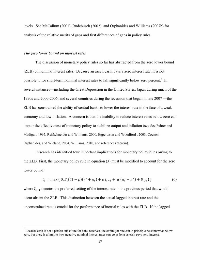
The discussion of monetary policy rules so far has abstracted from the zero lower bound

(ZLB) on nominal interest rates. Because an asset, cash, pays a zero interest rate, it is not

possible to for short-term nominal interest rates to fall significantly below zero percent.4 In

several instances—including the Great Depression in the United States, Japan during much of the

1990s and 2000-2006, and several countries during the recession that began in late 2007 —the

ZLB has constrained the ability of central banks to lower the interest rate in the face of a weak

economy and low inflation. A concern is that the inability to reduce interest rates below zero can

impair the effectiveness of monetary policy to stabilize output and inflation (see See Fuhrer and

Madigan, 1997, Reifschneider and Williams, 2000, Eggertsson and Woodford , 2003, Coenen ,

Orphanides, and Wieland, 2004, Williams, 2010, and references therein).

Research has identified four important implications for monetary policy rules owing to

the ZLB. First, the monetary policy rule in equation (3) must be modified to account for the zero

lower bound:

max 0, 1 ̃ (6)

where ̃ denotes the preferred setting of the interest rate in the previous period that would

occur absent the ZLB. This distinction between the actual lagged interest rate and the

unconstrained rate is crucial for the performance of inertial rules with the ZLB. If the lagged

                                                            4 Because cash is not a perfect substitute for bank reserves, the overnight rate can in principle be somewhat below zero, but there is a limit to how negative nominal interest rates can go as long as cash pays zero interest.

18  

interest rate appears in the rule, deviations from the unconstrained policy are carried into the

future, exacerbating the effects of the ZLB (Reifschneider and Williams 2000, Williams 2006).

Second, the ZLB can imply the existence of multiple steady states (Reifschneider and

Williams 2000, Benhabib, Schmitt-Grohe, and Uribe 2001). For a wide set of macroeconomic

models, one steady state is characterized by a rate of inflation equal to the negative of the

equilibrium real interest rate, a zero output gap zero, and a zero nominal interest rate. Assuming

the target inflation rate exceeds the negative of the equilibrium real interest rate, a second steady

state exists. It is characterized by a rate of inflation equal to the central bank’s target inflation

rate, a zero output gap, and a nominal interest rate equal to the equilibrium real interest rate plus

the target inflation rate. In standard models, the steady state associated with the target inflation

rate is locally stable in the sense that the economy returns to this steady state following a small

disturbance. But, due to the existence of the ZLB, if a large contractionary shock hits the

economy, monetary policy alone may not be sufficient to bring the inflation rate back to the

target rate. Instead, depending on the nature of the model economy’s dynamics, the inflation rate

will either converge to the deflationary steady state or will diverge to an infinitely negative

inflation rate. Fiscal policy can be used to eliminate the deflationary steady state and assure that

the economy returns to the desired steady state inflation rate (Evans, Guse, and Honkapohja,

2008).5

Third, the ZLB has implications for the specification and parameterization of the

monetary policy rule. For example, Reifschneider and Williams (2002) find that increasing the

response to the output gap helps reduce the effects of the ZLB. Such an aggressive response to

output gaps prescribes greater monetary stimulus before and after episodes when the ZLB

                                                            5 See also Eggertsson and Woodford (2006). In addition to fiscal policy, researchers have examined the use of alternative monetary policy instruments, such as the quantity of reserves, the exchange rate, and longer-term interest rates. See McCallum (2000), Svensson (2001), and Bernanke and Reinhart (2004) for discussions of these topics.

19  

constrains policy, which helps lessen the effects when the ZLB constrains policy. However,

there are limits to this approach. First, it generally increases the variability of inflation and

interest rates, which may be undesirable. In addition, Williams (2010) shows that too large a

response to the output gap can be counterproductive. The ZLB creates an asymmetry between

the very strong responses to positive output gaps and truncated responses to negative output gaps

that increases output gap variability overall.

Given the limitations of the approach of simply responding more strongly to output gaps,

Reifschneider and Williams (2000, 2002) argue for modifications to the specification of the

policy rule. They consider two alternative specifications of simple policy rules. In one, the

policy rule is modified to lower the interest rate more aggressively than otherwise in the vicinity

of the ZLB. In particular, they consider a rule where the interest rate is cut to zero if the

unconstrained interest rate falls below 1 percent. This asymmetric rule encapsulates the principle

of adding as much monetary stimulus as possible near the ZLB in order to offset the effects of

constraint on monetary stimulus when the ZLB binds. In the second version of the modified

rule, the interest rate is kept below the “notional” interest rate following episodes when the ZLB

is a binding constraint on policy. Specifically, the interest rate is kept at zero until the absolute

value of the cumulative sum of negative deviations of the actual interest rate from the notional

values equals that that occurred during the period that ZLB constrained policy. This approach

implies that the rule “makes up” afterwards for lost monetary stimulus resulting from the ZLB.

Both of these approaches work well at mitigating the effects of the ZLB in model

simulations when the public is assumed to know the features of the modified policy rule.

However, these approaches rely on unusual behavior by the central bank in the vicinity of the

ZLB, which may confuse private agents and thereby entail unintended and potentially

20  

undesirable consequences. An alternative approach advocated by Eggertsson and Woodford

(2003) is to adopt an explicit price-level target, rather than an inflation target. Reifschneider and

Williams (2000) and Williams (2006, 2010) find that such price-level targeting rules are

effective at reducing the costs of the ZLB as long as the public understands the policy rule. Such

an approach works well because, like the second modified policy rule discussed above, it

promises more monetary stimulus and higher inflation in the future than a standard inflation-

targeting policy rule. This anticipation of future monetary stimulus boosts economic activity and

inflation when the economy is at the ZLB, thereby mitigating its effects. This channel is highly

effective in models where expectations of future policy have important effects on current output

and inflation. But, as pointed out by Walsh (2009), central bankers have so far been unwilling to

embrace this approach in practice.

Finally, the ZLB provides an argument for a higher target inflation rate than otherwise

would be the case. The quantitative importance of the ZLB depends on the frequency and degree

to which the ZLB constraint is expected to bind, a key determinant of which is the target

inflation rate. If the target inflation rate is sufficiently high, the ZLB will rarely impinge on

monetary policy and the macroeconomy. As discussed in Williams (2010), the consensus from

the literature on the ZLB is that a 2 percent inflation target is sufficient to avoid significant costs

in terms of macroeconomic stabilization, based on the historical pattern of disturbances hitting

the economy over the past several decades. This figure is close to the inflation targets followed,

either explicitly or implicitly, by many central banks today (Kuttner 2004).

21  

Responding to other variables

A frequently-heard criticism of simple monetary policy rules is that they ignore valuable

information about the economy. In other words, they are simply too simple for the real-world

(Svensson 2003 and Mishkin 2007). However, as shown in Williams (2003), even in large-scale

macroeconometric models like FRB/US, adding additional lags or leads of inflation or the

output gap to the three-parameter rule of the type discussed above yields trivial gains in terms of

macroeconomic stabilization. The same is true for other empirical macro models (Rudebusch

and Svensson 1999, Levin and Williams 2003, Levin, Wieland, and Williams 1999). Similar

results are found using micro-founded DSGE models where the central bank aims to maximize

household welfare (Levin, Onatski, Williams, and Williams, 2005, Edge, Laubach, and

Williams, 2010).

One specific issue that has attracted a great deal of attention is adding various asset

prices, such as the exchange rate or equity prices, to the policy rule (see Clarida, Gali, and

Gertler, 2001, Bernanke and Gertler, 1999, and Woodford, 2003, for discussions and references).

Research has shown that he magnitude of the benefits from responding to asset prices is

generally found to be small in existing estimated models. For example, the FRB/US model

includes a wide variety of asset prices which may deviate from fundamentals. Nonetheless,

including asset price movements (or, alternatively, non-fundamental movements in asset prices)

to simple policy rules yields negligible benefits in terms of macroeconomic stabilization in this

model. One reason for this is that asset price movements unrelated to fundamentals lead to

movements in output and inflation in the model. The simple policy rule responds to and offsets

these movements in inflation and the output gap.6 Moreover, in practice it is difficult to

                                                            6 Of course, if the policy objective included the stabilization of asset prices, then the optimal simple rule

would need to contain the asset prices as well as the other objective variables.

22  

accurately measure nonfundamental movements in asset prices, arguing for muted responses to

these noisy variables.

3. Robustness of Policy Rules

Much of the early research focused on the performance of simple policy rules under

“ideal” circumstances where the central bank has an excellent knowledge of the economy and

expectations are rational. But, it had long been recognized that such assumptions are unlikely to

hold in real-world policy applications and that policy prescriptions needed to be robust to

uncertainty (McCallum 1988, Taylor 1993b). Research has therefore focused on the issue of

designing robust policy rules that perform well in a wide set of economic environments (see, for

example, Brock, Durlauf, and West, 2003, 2007, Brock, Durlauf, Nason, and Rondina , 2007,

Levin and Williams, 2003, Levin, Wieland, Williams, 1999, 2003, Orphandies and Williams,

2002, 2006, 2007b, 2008, Taylor and Wieland , 2009, and Tetlow, 2006).

Evaluating policy rules in a variety of models has the advantage of helping identify

characteristics of policy rules that are robust to model misspecification and those that are not.

Early efforts at evaluating robustness took the form of taking evaluating candidate policy rules

through a set of models and comparing the results with regard to macroeconomic performance.

Later, this approach was formalized as a problem of decision making under uncertainty.

One example of robustness evaluation is the joint effort of several researchers to compare

the effects of policy rules in different models, reported in Taylor (1999b). In that project, five

different candidate policy rules were checked for robustness across a variety of models. These

policy rules were of the form of equation (3); the parameters are reported in Table 1. Note that

the interest rate reacts to the lagged interest rate with a coefficient of one in Rules I and II, with

23  

Rule I having higher weight on inflation compared to output and Rule II has a smaller weight on

inflation compared to output. Thus these two rules have considerable “inertia” in the terminology

used above. Rule III is the Taylor Rule. Rule IV has a coefficient of 1.0 rather than 0.5 on real

output, which had been suggested by Brayton, Levin, Tryon, and Williams (1997). Rule V is the

rule proposed by Rotemberg and Woodford (1999); it places very little weight on real output and

incorporates a greater than unity coefficient on the lagged interest rate.

Table 1

Policy Rule Coefficients _____________α_____β_____ ρ___

Rule I 3.0 0.8 1.0 Rule II 1.2 1.0 1.0 Rule III 0.5 0.5 0.0 Rule IV 0.5 1.0 0.0 Rule V 1.5 .06 1.3

_____________________________

In this exercise, nine models were considered (see Taylor 1999b). For each of the

models, the standard deviations of the inflation rate, of real output, and of the interest rate were

computed. Taylor (1999b) reports that the sum of the ranks of the three rules shows that Rule I

is most robust if inflation fluctuations are the sole measure of performance; it ranks first in terms

of inflation variability for all but one model for which there is a clear ordering. For output, Rule

II has the best sum of the ranks, which reflects its relatively high response to output. However,

regardless of the objective function weights, Rule V has the worst sum of the ranks of these three

policy rules, ranking first for only one model (the Rotemberg-Woodford model) in the case of

output. Comparing rules I, II, III with Rules III and IV) shows that the lagged interest rate rules

24  

do not dominate rules without a lagged interest rate. Indeed, for a number of models the rules

with lagged interest rates are unstable or have extraordinarily large variances.

This type of exercise has been expanded to include other models and to formally search

for the “best” simple rule evaluated over a set of models. One issue that this literature has faced

is the characterization of the problem of optimal policy under uncertainty. Different approaches

have been used, including Bayesian, minimax, and minimax regret (see Brock, Durlauf, and

West, 2003, and Kuester and Wieland, 2010, for detailed discussions).

The Bayesian approach assumes that the existence of well-defined probabilities, pj, for

each model j in a set of n models The choice of the optimal rule under uncertainty then is the

choice of the parameters of the rule that minimizes the expected loss over the set of models. In

particular, denote the central bank loss generated in model j by Lj. The Bayesian central bank’s

expected loss, LB, is given by:

∑ . (7)

This formulation treats the probabilities as constant; see Brock, Durlauf, and West 2003 for the

description of the expected loss in a dynamic context where the probabilities are updated each

period.

Levin and Williams (2003) apply this methodology to a set of three models taken from

Woodford (2003), Fuhrer (2000), and Rudebusch and Svensson (1999). They place equal

probabilities on these three models. They find that the Bayesian optimal simple three-parameter

rule is characterized by a moderate degree of policy inertia, with ρ no greater than 0.7. In the

two forward-looking models, the optimal response to the lagged interest rate is much higher than

0.7. In contrast, in the backward-looking Rudebusch-Svensson model, the optimal policy is

25  

characterized by very little inertia. In fact, in that model, highly inertial policies can lead to

explosive behavior.

The robustness of simple rules to alternative parameterizations can be illustrated using

the concept of fault tolerance (Levin and Williams 2003). Figure 5 plots percent the deviations of

the central bank loss relative to the fully optimal policies for the three models studied by Levin

and Williams for variations in the three parameters of the policy rule. This figure shows results

for the case of λ = 0. The upper panel shows how the central bank loss changes in the three

models as the value of ρ ranges from 0 to 1.5. In constructing these curves, the other two

parameters of the policy rule are held constant at their respective optimal values. The middle and

bottom panels show the results when the coefficient on inflation and the output gap, respectively,

are varied. In cases where the curves are relatively flat, the policy is said to be fault tolerant,

meaning that model misspecification does not lead to a large increase in loss relative to what

could be achieved. If the curve is steep, the policy is said to be fault intolerant. Robust policies

are those that lie in the fault tolerant regions of the set of models under consideration.

As seen in the figure, inertial policies lead to very large increases in the central bank loss

in the Rudebusch-Svensson model. And highly inertial policies with values of ρ greater than one

are damaging in the Fuhrer model as well. The reason for this result in the Rudebusch-Svensson

models is that monetary policy effects grow slowly over time and there is no feedback of these

future effects of policy back onto the current economy. A highly inertial policy will be behind

the curve in shifting the stance of policy, amplifying fluctuations and potentially leading to

explosive oscillations. In forward-looking models, in contrast, expected future policy actions

help stabilize the current economy, which reduces the need for large movements in interest rates.

26  

Nonetheless, excessive policy inertia with ρ > 1 is undesirable in forward-looking models with

strong real and nominal frictions such as the Fuhrer model and FRB/US.

The choice of the responses to inflation and the output gap can be quite different when

viewed from the perspective of robustness across models rather than optimality in a single

model. For example, in the case shown here, macroeconomic performance in the Fuhrer model

suffers when the response to inflation is too great. The case of the optimal response to the output

illuminates the tension between optimal and robust policies. In two of the models, the optimal

response is near zero. However, such a response is highly costly in the third (Rudebusch-

Svensson) model. Similarly, the relatively large response to the output gap called for by the

Rudebusch-Svensson model performs poorly in the other two models. Evidently, the robust

policy differs significantly from each optimal policy by having a modest response to the output

gap that is suboptimal in each model, but highly costly in none.

Orphanides and Williams (2006) conduct a robustness analysis, where the uncertainty is

over the way that agents form expectations and the magnitude of fluctuations in the equilibrium

real interest rate and the natural rate of unemployment. Figure 6 plots the fault tolerances for

three models that they study. For this exercise, the coefficient on the lagged interest rate was set

to zero. In one model, labeled “perfect knowledge,” private agents possess rational expectations

and the equilibrium real interest rate and the natural rate of unemployment are constant and

known. The second model, labeled ‘learning,” replaces the assumption of rational expectations

with the assumption that private agents form expectations using an estimated forecasting model.

The third model, labeled “learning + natural rate misperceptions,” adds uncertainty about the

equilibrium real interest rate and the natural rate of unemployment to the model with learning.

27  

The optimal policy in the “perfect knowledge” model performs poorly in the models with

learning and natural rate misperceptions. In particular, as seen in the upper panel of the figure,

the “perfect knowledge” model prescribes a modest response to inflation in the policy rule. Such

a policy is highly problematic in the other models with learning because it allows inflation

expectations to drift over time. The optimal policies in the models with learning feature much

stronger responses to inflation and thereby tighter control of inflation expectations. Such policies

engender relatively small cost in performance in the “perfect knowledge” model and represent a

robust strategy for this set of models.

As mentioned above, the Bayesian approach to policy rule evaluation under model

uncertainty requires one to specify probabilities on the various models. In practice, this may be

difficult or impossible to do. In such cases, alternative approaches are minimiax and minimax

regret. The minimiax criterion, LM, is given by:

max , , … , . (8)

Levin and Williams (2003) and Kuester and Wieland (2010) analyze the properties of minimax

simple rules. One problem with this approach is that it can be very sensitive to outlier models.

Hybrid approaches such as that of Kuester and Wieland (2010) and ambiguity aversion described

by Brock, Durlauf, and West (2003) allow one to combine the Bayesian approach with

robustness to “worst-case” models. This is done less formally by examining the performance of

the candidate policy not only in terms of the average performance across the models, but also in

each individual model.

A recurring result in the literature is that optimal Bayesian policy rules entail relatively

small stabilization costs, relative to the optimal policy, in nearly all the models in the set (see

Levin and Williams, 2003, Levin, Wieland, Williams, 1999, 2003, Orphandies and Williams,

28  

2002, 2008, and references therein). That is, the cost of robustness to model uncertainty tends to

be relatively small, while the benefits can be very large.

4. Optimal Policy vs. Simple Rules

An alternative approach to that of simple monetary policy rules is that of optimal policy

(Giannoni and Woodford, 2005, Svensson, 2010, Woodford, 2010). The optimal policy

approach treats the monetary policy problem as a standard intertemporal optimization problem,

which yields optimalilty conditions in terms of first-order conditions and Lagrange multipliers.

As discussed in Giannoni and Woodford (2005), the optimal policy can be formulated as a single

equation in terms of leads and lags of the objective variables (inflation rate, output gap, etc.). A

key theoretical advantage of the optimal policy approach is that it, unlike simple monetary policy

rules, takes into account all relevant information for monetary policy.

The value of this informational advantage has been found to be surprisingly small in

model simulations, even when the central bank is assumed to have perfect knowledge of the

model. Of course, in small enough models, the optimal policy may be equivalent to a simple

policy rule, as in Ball (1999). But, in larger models, this is no longer the case. Williams (2003),

using the large-scale Federal Reserve Board FRB/US model, finds that a simple three-parameter

monetary policy rule yields outcomes in terms of the weighted sum of variances of the inflation

rate and the output gap that are remarkably close to those obtained under the fully optimal

policy. This result is illustrated in Figure 4, which shows the policy frontiers from the FRB/US

model between the fully optimal policy and the three-parameter rule. For a policymaker who

cares equally about inflation and the output gap (λ = 1), the standard deviations of both the

inflation rate and the output gap are less than 0.1 percentage point apart between the frontiers.

29  

Similar results are obtained for a wide variety of estimated macroeconomic models

(Rudebusch and Svensson, 1999, Levin and Williams, 2003, Levin, Onatski, Williams, and

Williams, 2005, Schmitt-Grohe and Uribe, 2006, Edge, Laubach, and Williams 2010). Giononni

and Woodford (2005) provide the theoretical basis for why simple rules perform so well. They

show that the fully optimal policy can be described as a relationship between leads and lags of

the variables in the loss function. Evidently, simple rules of the type studied in the literature

capture the key aspects of this relationship between the objective variables.

One potential shortcoming of the optimal control approach is that it ignores uncertainty

about the specification of the model (see McCallum and Nelson 2005 for a discussion).

Although in principle one can incorporate various types of uncertainty to the analysis of optimal

policy, in practice computational feasibility limits what can be done. As a result, existing

optimal control policy analysis is typically done using a single reference model, which is

assumed to be true.

Levin and Williams (2003) and Orphanides and Williams (2008) find that optimal

policies can perform very poorly if the central bank's reference model is misspecified, while

simple robust rules perform well in a wide variety of models, as discussed above. This research

provides examples where optimal polices can be overly fine tuned to the particular assumptions

of the model. If those assumptions prove to be correct, all is well. But, if the assumptions turn

out to be false, the costs can be high. In contrast, simple monetary policy rules are designed to

take account of only the most basic principle of monetary policy of leaning against the wind of

inflation and output movements. Because they are not fine tuned to specific assumptions, they

are more robust to mistaken assumptions. Figure 7, taken from Orphanides and Williams (2008),

illustrates this point. The optimal control policy derived under the assumption of rational

30  

expectations performs slightly better than the two simple rules if the model where expectations

are in fact rational. But, in the alternative models where agents form expectations using

estimated forecasting models, indexed by the learning parameter κ, the performance of the

optimal control policy deteriorates sharply while that of the simple rules holds up well.

One potential solution to this lack of robustness is to design optimal control rules that are

more robust to model misspecification. One such approach is to use robust control techniques

(Hansen and Sargent 2007). A n alternative approach is to bias the objective function so that the

optimal control policy is more robust to model uncertainty. The results for such a “modified

optimal policy” is shown in Figure 5. In this case, the modification is to reduce the weights

placed on stabilizing unemployment and interest rates in the objective function when computing

the optimal policy (see Orphanides and Williams 2008 for a discussion). Interestingly, although

this policy is more robust than the standard optimal policy, overall it doesn’t do as well as the

optimal simple inertial rule, as seen in the figure.

A final issue with optimal policies is that they tend to be very complicated and potentially

difficult to communicate to the public, relative to simple rules. In an environment where the

pubic lacks a perfect understanding of the policy strategy, this complexity may make it harder for

private agents to learn, creating confusion and expectational errors, as discussed by Orphanides

and Williams (2008).

These robustness studies characterize optimal policy in terms of an optimal feedback

rule—a function relating policy instruments to lagged policy instruments and other observable

variables in such a way that the objective function is maximized for a particular model. This

optimal feedback rule is then compared with simple (not fully optimal) rules by simulating the

rules in different models. There are a variety of ways other than feedback rules to characterize

31  

optimal policy. For example, as mentioned above the policy instruments could depend on

forecasts of future variables, as discussed by Giannoni and Woodford (2005). In general there

are countless ways of representing optimal policy in a given model. When simulating how

optimal policy works in a different model, the results could depend on which of these

representations of optimal policy one uses An open question, therefore, is whether one

characterization of optimal policy might be more robust than those studied so far.

5. Learning from Experience Before, During and After the Great Moderation

Another approach to learn about the usefulness of simple policy rules is look at actual

macroeconomic performance when policy operates, or does not operate, close to such rules. The

Great Moderation period is good for this purpose because economic performance was unusually

favorable during that period, either compared to the period before or, so far at least, the period

after.

By all accounts the Great Moderation in the United States began in the early 1980s. In

particular, it is reasonable to date the beginning of the Great Moderation with the first month of

the expansion following the 1981-82 recession (November 1982) and to date its end at the

beginning of the 2007-09 recession (December 2007). Not only did inflation and interest rates

and their volatilities diminish compared with the experience of the 1970s, but the volatility of

real GDP reached lows never seen before. Economic expansions became longer and stronger

while recessions became shorter and shallower. No matter what metric you use—the variance of

real GDP growth, the variance of the real GDP gap, the average length of expansions, the

frequency of recessions, or the duration of recessions—there was a huge improvement in

economic performance. There was also an improvement in price stability with the inflation rate

32  

much lower and less volatile than the period from the late 1960s to the early 1980s. This same

type of improved macroeconomic performance also occurred in other developed countries and

most developing countries (Cecchetti, Flores-Lagunes, and Krause, 2006).

Is there evidence that policy adhered more to simple policy rules during the Great

Moderation? Yes. Indeed the evidence shows that not only the Fed, but also many other central

banks became markedly more responsive and systematic in adjusting to developments in the

economy when changing their policy interest rate. This is a policy regime change in the

econometric sense: one can observe it by estimating, during different time periods, the

coefficients of the central bank’s policy rule which describes of how the central bank sets its

interest rate in response to inflation and real GDP.

A number of researchers used this technique to detect a regime shift, including Judd and

Rudebusch (1998), Clarida, Gali, and Gertler (2000), Woodford (2003), and Stock and Watson

(2002). Such studies have shown that the Fed’s interest rate moves were less responsive to

changes in inflation and to real GDP in the period before the 1980s. After the mid 1980s, the

reaction coefficients increased significantly. The reaction coefficient to inflation nearly doubled.

The estimated reaction of the interest rate to a one percentage point increase in inflation rose

from about three-quarters to about one-and-a-half. The reaction to real output also rose. In

general the coefficients are much closer to the parameters of a policy rule like the Taylor rule in

the post mid-1980s period than they were before. Similar results are found over longer sample

periods for the United States. The implied reaction coefficients were also low in the highly

volatile pre-World War II period (Romer and Romer 2002).

33  

Cecchetti et al (2007) and others have shown that this same type of shift occurred in other

countries. They pinpoint the regime shift as having occurred for a number of countries in the

early 1980s by showing that deviations from a Taylor rule began to diminish around that time.

While this research establishes that the Great Moderation and the change in policy rules

began about the same time, it does not prove they are connected. Formal statistical techniques or

macroeconomic model simulation can help assess causality. Stock and Watson (2002) used a

statistical time-series decomposition technique to assess the causality. They found that the

change in monetary policy had an effect on performance, though they also found that other

factors—mainly a reduction in other sources of shocks to the economy (inventories, supply

factors)—were responsible for a larger part of the reduction in volatility. They showed that the

shift in the monetary policy rule led to a more efficient point on the output-inflation variance

tradeoff. Similarly, Cecchetti, Flores-Lagunes, and Krause (2006) used a more structural model

and empirically studied many different countries. For 20 of the 21countries which had

experienced a moderation in the variance of inflation and output, they found that better monetary

policy accounted for over 80 percent of the moderation.

Some additional evidence comes from establishing a connection between the research on

policy rules and the decisions of policy makers. Asso, Kahn, and Leeson (2007) have

documented a large number of references to policy rules and related developments in the

transcripts of the FOMC in the 1990s. Meyer (2004) makes it clear that there was a framework

underlying the policy based on such considerations. If you compare Meyer’s (2004) account with

Maisel’s (1973), you see a very clear difference in the policy framework.

So far we have considered evidence in favor of a shift in the policy rule and improved

economic performance during the Great Moderation. Is it possible that the end of the Great

34  

Moderations was due to another monetary policy shift? In thinking about this question, it is

important to recall that the Great Moderation was already nearly 15 years old before economists

started noticing it, documenting it, determining the date of its beginning, and trying to determine

whether or not it was due to monetary policy. It will probably take as long to draw definitive

conclusions about the end of the Great Moderation, and after all we hope that Great Moderation

II will start soon. Nevertheless, Taylor (2007) provides evidence that in 2003-2005, policy

deviated from the policy rule that worked well during the Great Moderation.

Rules as Measures of Accountability

This review of historical performance distinguishes periods when policy is close to a

policy rule and when it is not. In other words, it focuses on whether or not there is a deviation

from a policy rule. In a sense, such deviations from policy rules—at least large persistent

deviations—can serve as measures of accountability for monetary policy makers. Congressional

or parliamentary committees sometimes use such measures when questioning central bankers,

and public debates over monetary policy decisions are frequently about whether policy is

deviating from a policy rule or not.

It is important to point out that using policy rules in this way, while quite natural, was not

emphasized in the many of the original proposals for interest rate rules, such as the one in Taylor

(1993a). Rather the policy recommendation was that the rule should be used as an aid for

making decisions in a more predictable, rule-like, manner: Accordingly, the Federal Reserve

staff would show to the FOMC the paths of the federal funds rate under the Taylor rule and other

policy rules, and the FOMC would then use the information in making the decision about

35  

whether or not to change the interest rate. Policy rules would thus inform policy decisions; it

would serve as a rough benchmark for making decisions not a mechanical formula. As Kohn

(2007) has described in his analysis of the 2002-2004 period and the response to Taylor (2007),

this is how policy rules came to be used at the FOMC.

The rationale for using deviations from policy rules as measures of accountability came

later and is based on historical and international experience over the past two decades. Historical

work has shown that there were big deviations from policy rules at the times that performance

was less than satisfactory. A question is whether in the future policy rules will be used more

often in this more specific way as a measure of accountability rather than as simply a guide or

aid for policy decisions. If rules become more commonly used for accountability, then policy

makers will have to explain the reasons for the deviations from the rules and be held accountable

for them. As stated by Levin and Taylor (2009) “on occasion, of course, policymakers might

find compelling reasons to deviate from the prescriptions of any simple rule, but in those

circumstances, transparency and credibility might well call for clear communication about the

rationale for that policy strategy.”

Conclusion

Research on rules for monetary policy rules over the past two decades has made

important progress in understanding the properties of simple policy rules and their robustness to

model misspecification. Simple normative rules to guide central bank decisions for the interest

rate first emerged from research on simulations of empirical monetary models with rational

expectations and sticky prices in the 1970s and 1980s; this research built on work going back to

Smith, Ricardo, Fisher, Wicksell, and Friedman in the sense that the research objective was to

36  

find a monetary policy which both cushioned the economy to shocks and did not cause its own

shocks.

Over the past two decades, research on policy rules has shown that simple rules have

important robustness advantages over fully optimal or more complex rules in that they work well

in a variety of models. Experience has shown that simple rules also have worked well in the real

world. Progress has also been made in understanding how to adjust simple rules to deal with

measurement error, expectations, learning, and the lower bound on interest rates. That said, the

search for better and more robust policy rules is never done and further research is needed that

incorporates a wider set of models and economic environments, especially models that take

account international linkages of monetary policy and economies. In addition, many of the

studies of robustness have looked at only a handful of models in isolation from all the other

potential models. A desirable goal is to include large numbers of alternative models in one

study. Another goal of future research should be to gain a better understanding of the

implications of deviations from policy rules due to discretionary policy actions.

37  

References

Asso, Francesco, George Kahn, and Robert Leeson (2007) “Monetary Policy Rules: from Adam

Smith to John Taylor,” presented at Federal Reserve Bank of Dallas Conference, October

2007 http://dallasfed.org/news/research/2007/07taylor_leeson.pdf

Ball, Lawrence (1999) “Efficient Rules for Monetary Policy,” International Finance, Vol. 2, No.

1, 63-83.

Batini, Nicoletta and Andrew Haldane (1999). “Forward-Looking Rules for Monetary Policy,” in

John B. Taylor, ed., Monetary Policy Rules, Chicago: University of Chicago Press, 157–

92.

Benhabib, Jess, Stephanie Schmitt-Grohe, and Matin Uribe (2001), “The Perils of Taylor Rules,”

Journal of Economic Theory, 96(1-2), January, 40-69.

Bernanke, Ben, and Mark Gertler (1999), Monetary Policy and Asset Price Volatility,”

Federal Reserve Bank of Kansas City Economic Review, Fourth quarter, 18-51.

Bernanke, Ben S., and Vincent R. Reinhart (2004), “Conducting Monetary Policy at Very Low

Short-Term Interest Rates,” American Economic Review, Papers and Proceedings, 94(2),

85-90.

Brayton, Flint, Andrew Levin, Ralph Tryon, and John C. Williams (1997), “The Evolution of

Macro Models at the Federal Reserve Board,” Carnegie-Rochseter Conference Series on

Public Policy, December, 47, 43-81.

Brock, William A., Steven N. Durlauf, James Nason, and Giacomo Rondina (2007),” Journal of

Monetary Economics, 54(5), 1372-1396.

Brock, William A., Steven N. Durlauf, and Kenneth D. West (2003), “Policy Analysis in

Uncertain Economic Environments,” Brookings Papers on Economic Activity, 1, 235-

322.

Brock, William A., Steven D. Durlauf, and Kenneth D. West (2007), “Model Uncertainty and

Policy Evaluation: Some Theory and Empirics,” Journal of Econometrics, 136, 2, 629-

664.

Bryant, Ralph, Peter Hooper and Catherine Mann (1993), Evaluating Policy Regimes: New

Empirical Research in Empirical Macroeconomics, Brookings Institution, Washington,

D.C.

38  

Cecchetti, Stephen G., Alfonso Flores-Lagunes, and Stefan Krause (2006) “Has Monetary Policy

Become More Efficient? A Cross-country Analysis” Economic Journal, Vol. 116, No.

115, pp. 408-433.

Cecchetti, Stephen G., Peter Hooper, Bruce C. Kasman, Kermit L. Schoenholtz, and Mark W.

Watson (2007), “Understanding the Evolving Inflation Process,” presented at the U.S.

Monetary Policy Forum 2007.

Clarida, Richard, Jordi Gali, and Mark Gertler (2000), “Monetary Policy Rules and

Macroeconomic Stability: Evidence and Some Theory,” Quarterly Journal of Economics

(February), 115, 1, 147-180.

Clarida, Richard, Jordi Gali, and Mark Gertler (2001), “Optimal Monetary Policy in Open

Versus Closed Economics: An Integrated Approach,” American Economic Review

Papers and Proceedings, 91, May, 248-252.

Coenen , Guenter, Athansios Orphanides, and Volker Wieland (2004), “Price Stability and

Monetary Policy Effectiveness when Nominal Interest Rates are Bounded at Zero,”

Advances in Macroeconomics, 4(1).

Dewald, William G., and Harry G. Johnson (1963), ``An Objective Analysis of the Objectives of

American Monetary Policy, 1952-61,'' in Banking and Monetary Studies, edited by

Deane Carson, 171-189. Homewood, Illinois: Richard D. Irvin.

Edge, Rochelle M., Thomas Laubach, and John C. Williams (2010), “Welfare-Maximizing

Monetary Policy under Parameter Uncertainty,” Journal of Applied Econometrics, 25,

January/February, 129-143.

Eggertsson, Gauti B., and Michael Woodford (2003), “The Zero Interest-Rate Bound and

Optimal Monetary Policy,” Brookings Papers on Economic Activity, 1, 139-211.

Eggertsson, Gauti B., and Michael Woodford (2006), ``Optimal Monetary and Fiscal Policy in a

Liquidity Trap,” NBER International Seminar on Macroeconomics 2004, Richard H.

Clarida, Jeffrey Frankel, Francesco Giavazzi and Kenneth D. West, eds., Cambridge,

MA.: MIT Press, 75-131.

Evans, George W., Eran Guse, and Seppo Honkapohja (2008), “Liquidity Traps, Learning and

Stagnation,” European Economic Review, 52, 1438 – 1463.

39  

Fair, Ray C. (1978), “The Sensitivity of Fiscal Policy Effects to Assumptions about the Behavior

of the Federal Reserve,”' Econometrica, 46, 1165-1179.

Fair, Ray C. and Howrey, E. Philip (1996), “Evaluating Alternative Monetary Policy Rules,”

Journal of Monetary Economics, 38(2), 173--193.

Fuhrer, Jeffrey C. (1997), Inflation/Output Variance Trade-offs and Optimal Monetary Policy.''

Journal of Money, Credit and Banking, May, 29(2), 214-234.

Fuhrer, Jeffrey C. (2000), “Habit Formation in Consumption and Its Implications for Monetary-

Policy Models,” American Economic Review, June, 90(3), 367-90.

Fuhrer, Jeffrey C., and Brian Madigan (1997), “Monetary Policy when Interest Rates are

Bounded at Zero,” Review of Economics and Statistics, 79, November, 573-85.

Giannoni, Marc P. and Michael Woodford (2005), “Optimal Inflation Targeting Rules,'' In:

Bernanke, B.S., Woodford, M. (Eds.), The Inflation Targeting Debate, Chicago:

University of Chicago Press, 93—162.

Hansen, Lars Peter, and Thomas J. Sargent (2007), Robustness, Princeton University Press .

Henderson, Dale W., and Warwick J. McKibbin (1993), “An Assessment of Some Basic

Monetary Policy Regime Pairs: Analytical and Simulation Results from Simple Multi-

Region Macroeconomic Models,” in R. Bryant, P. Hooper, and C. Mann (eds),

Evaluating Policy Regimes: New Research in Empirical Macroeconomics, Brookings

Institution, Washington, D.C., 45–218.

Judd, John, and Glenn D. Rudebusch (1998), “Taylor's Rule and the Fed: 1970-1997,” Federal

Reserve Bank of San Francisco Economic Review 3, pp. 1-16.

Kohn, Donald (2007), “John Taylor Rules,” paper presented at a conference at the Federal

Reserve Bank of Dallas, October, 2007.

Kuester, Keith, and Volker Wieland (2010), “Insurance Policies for Monetary Policy in the Euro

Area,” Journal of the European Economic Association.

Kuttner, Kenneth N. (2004), “A Snapshot of Inflation Targeting in its Adolescence,” in

Christopher Kent and Simon Guttmann (ed.), The Future of Inflation Targeting, Sydney,

Australia: Reserve Bank of Australia, November, 6-42.

Kydland, Finn E., and Edward C. Prescott (1977), “Rules Rather Than Discretion: The

Inconsistency of Optimal Plans,” Journal of Political Economy, 85(3), 473–491.

40  

Laubach, Thomas and John C. Williams (2003), “Measuring the Natural Rate of Interest,”

Review of Economics and Statistics, 85(4), November, 1063-1070.

Levin, Andrew T., Alexei Onatski, John C. Williams, and Noah Williams (2005), “Monetary

Policy Under Uncertainty in Micro-Founded Macroeconometric Models,” NBER

Macroeconomics Annual 2005, 229-289.

Levin, Andrew T., and John B. Taylor (2009), “Falling Behind the Curve: A Positive Analysis

of Stop-Start Monetary Policies and the Great Inflation,” NBER Working Paper.

Levin, Andrew T., Volker Wieland, and John C. Williams (1999), "Robustness of Simple

Monetary Policy Rules under Model Uncertainty." In Monetary Policy Rules, John B.

Taylor (Ed), pp. 263-299. Chicago: Chicago University Press.

Levin, Andrew T., Volker Wieland, and John C. Williams (2003), “The performance of forecast-

based policy rules under model uncertainty,” American Economic Review, 93 (3), 622–

645.

Levin, Andrew T., and John C. Williams (2003), “Robust Monetary Policy with Competing

Reference Models,” Journal of Monetary Economics, 50, 945--975.

Lucas, Robert E., Jr. (1976), “Econometric Policy Evaluation: A Critique,” Carnegie Rochester

Conference Series on Public Policy, 1, 19-46.

Maisel, Sherman J. (1973), Managing the Dollar, W.W. Norton, New York.

McCallum, Bennett T. (1988), “Robustness Properties of a Rule for Monetary Policy,” Carnegie-

Rochester Conference Series on Public Policy, Autumn, 29, 173--203.

McCallum, Bennett T. (1999) “Issues in the Design of Monetary Policy Rules,” Handbook of

Macroeconomics, John B. Taylor and Michael Woodford (eds).

McCallum, Bennett T. (2000), “Theoretical Analysis Regarding a Zero Lower Bound on

Nominal Interest Rates,” Journal of Money, Credit and Banking, 32(4), November.

McCallum, Bennett T. (2001), “Should Monetary Policy Respond Strongly to Output Gaps?''

American Economic Review Papers and Proceedings, 91(2), May, 258-62.

McCallum, Bennett T., and Edward Nelson (2005), “Targeting versus Instrument Rules for

Monetary Policy,” Federal Reserve Bank of St. Louis Review, September/October, 87(5),

597-611.

McNees, Stephen K. (1986), “Modeling the Fed: A Forward-Looking Monetary Policy Reaction

Function,” New England Economic Review, November/December, 3-8.

41  

Meyer, Laurence (2004), A Term at the Fed: An Insider’s View, HarperCollins, New York.

Meyer, Laurence (2009), “Dueling Taylor Rules,” unpublished paper, August.

Mishkin, Frederick (2007), “Housing and the Monetary Policy Transmission Mechanism,”

Federal Reserve Bank of Kansas City, Jackson Hole Conference.

Orphanides, Athanasios (1998), “Monetary Policy Evaluation with Noisy Information,” Board of

Governors of the Federal Reserve System, FEDS 1998-50, October.

Orphanides, Athanasios (2001), “Monetary Policy Rules Based on Real-Time Data,” American

Economic Review, 91(4), September, 964-985.

Orphanides, Athanasios (2002), "Monetary Policy Rules and the Great Inflation", American

Economic Review, Papers and Proceedings, 92(2), 115-120, May.

Orphanides, Athanasios (2008), “Taylor rules,” in S.N. Durlauf and L. E. Blume (eds) The New

Palgrave, Second Edition, New York: Palgrave Macmillian.

Orphanides, Athanasios, Richard D. Porter, David Reifschneider, Robert Tetlow, and Frederico

Finan (2000), “Errors in the Measurement of the Output Gap and the Design of Monetary

Policy,” Journal of Economics and Business, 52(1-2), 117–41.

Orphanides, Athanasios and Simon van Norden (2002), “The Unreliability of Output Gap

Estimates in Real Time,” Review of Economics and Statistics, 84(4), 569-583, November.

Orphanides, Athanasios and John C. Williams (2002). “Robust Monetary Policy Rules with

Unknown Natural Rates.” Brookings Papers on Economic Activity, 2:2002, 63-118.

Orphanides, Athanasios and John C. Williams (2006), "Monetary Policy with Imperfect

Knowledge,” Journal of the European Economic Association, 4(2-3), 366-375.

Orphanides, Athanasios and John C. Williams (2007a), “Inflation Targeting under Imperfect

Knowledge,” in Frederic Mishkin and Klaus Schmidt-Hebbel (ed.) Monetary Policy

under Inflation Targeting, Central Bank of Chile.

Orphanides, Athanasios and John C. Williams (2007b), “Robust Monetary Policy with Imperfect

Knowledge,” Journal of Monetary Economics 54, August, 1406-1435.

Orphanides, Athanasios and John C. Williams (2008) “Learning, Expectations Formation, and

the Pitfalls of Optimal Control Monetary Policy,” Journal of Monetary Economics, Vol.

55S, pp. S80-S96, October.

42  

Orphanides, Athanasios, and John C. Williams (2010), “Monetary Policy Mistakes and the

Evolution of Inflation Expectations,” Federal Reserve Bank of San Francisco Working

Paper, April.

Patinkin, Don (1956), Money, Interest and Prices: An Integration of Monetary and Value

Theory, Evanston: Row, Peterson.

Reifschneider, David L. and John C. Williams (2000), “Three Lessons for Monetary Policy in a

Low Inflation Era,” Journal of Money, Credit and Banking, 32(4), November, 936-966.

Reifschneider, David L. and John C. Williams (2002), “FOMC Briefing,” Board of Governors

of the Federal Reserve System, January.

Romer, Christina D., and David H. Romer (2002), “A Rehabilitation of Monetary Policy in The

1950's,” American Economic Review, 92(2), May, 121-127.

Rotemberg, Julio and Michael Woodford (1997), “An Optimization-Based Econometric

Framework for the Evaluation of Monetary Policy,” NBER Macroeconomics Annual, Ben

S. Bernanke and Julio Rotemberg (Eds.) pp. 297 – 361.

Rotemberg, Julio J. and Woodford, Michael (1999), ``Interest-Rate Rules in an Estimated Sticky

Price Model.'' in John B. Taylor, ed., Monetary Policy Rules, Chicago: University of

Chicago Press, 57-119.

Rudebusch, Glenn D. (2001), “Is the Fed Too Timid? Monetary Policy in an Uncertain World,”

Review of Economics and Statistics, 83, May, pp. 203-217.

Rudebusch, Glenn D. (2002), “Assessing Nominal Income Rules for Monetary Policy with

Model and Data Uncertainty,” The Economic Journal, 112, 402-432.

Rudebusch, Glenn D. (2006), “Monetary Policy Inertia: Fact or Fiction?” International Journal

of Central Banking, 2(4), December, 85-135.

Rudebusch, Glenn D. and Svensson, Lars E. O. (1999). “Policy Rules for Inflation Targeting,”

in John B. Taylor, ed., Monetary Policy Rules, Chicago: University of Chicago Press,

203-53.

Schmitt-Grohe, Stephanie and Martin Uribe (2007), “Optimal Simple and Implementable

Monetary and Fiscal Rules,” Journal of Monetary Economics, 54 (6), September, 1702-

1725.

43  

Smets, Frank (1999), “Output Gap Uncertainty: Does it matter for the Taylor Rule?” in:

Benjamin Hunt and Adrian Orr, eds., Monetary Policy under Uncertainty, Wellington,

New Zealand: Reserve Bank of New Zealand, 10--29.

Stock, James and Mark Watson (2002), “Has the Business Cycle Changed,” in Monetary Policy

and Uncertainty: Adapting to a Changing Economy, Jackson Hole Conference, Federal

Reserve Bank of Kansas City, pp 9-56.

Svensson, Lars E. O. (1999), “Price-Level Targeting vs. Inflation Targeting: A Free Lunch?''

Journal of Money, Credit and Banking, 31, 277-295.

Svensson, Lars E.O. (2001), “The Zero Bound in an Open Economy: A Foolproof Way of

Escaping from a Liquidity Trap,” Monetary and Economic Studies, 19(S-1), February,

277-312.

Svensson, Lars E.O. (2003), “What Is Wrong with Taylor Rules? Using Judgment in Monetary

Policy through Targeting Rules,” January, Journal of Economic Literature, 41, 426-477.

Svensson, Lars E.O. (2010), “Inflation Targeting,” prepared for Handbook of Monetary

Economics.

Taylor, John B. (1979), “Estimation and Control of a Macroeconomic Model with Rational

Expectations,” Econometrica, 47, September 1979.

Taylor, John B (1993a). “Discretion versus Policy Rules in Practice,” Carnegie Rochester

Conference Series on Public Policy, 39, 195-214.

Taylor, John B (1993b), Macroeconomic Policy in a World Economy: From Econometric Design

to Practical Operation, W.W. Norton, New York.

Taylor, John B. (1999a), Monetary Policy Rules, (Editor), University of Chicago Press.

Taylor, John B (1999b), “The Robustness and Efficiency of Monetary Policy Rules as

Guidelines for Interest Rate Setting by the European Central Bank,” Journal of Monetary

Economics, June, 43(3), 655-79.

Taylor, John B. (2007), ``Housing and Monetary Policy,'' In: Housing, Housing Finance, and

Monetary Policy, Kansas City, MO: Federal Reserve Bank of Kansas City, 463-476.

Taylor, John B., and Volker Wieland (2009), “Surprising Comparative Properties of Monetary

Models: Results from a New Data Base,” NBER Working Papers 14849, National Bureau

of Economic Research.

44  

Taylor, John B., and Michael Woodford (Editors), (1999), Handbook of Macroeconomics,

Elsevier.

Tetlow, Robert J. (2006), “Real-time Model Uncertainty in the United States: ‘Robust’ policies

put to the test,” mimeo, Federal Reserve Board, May 22.

Walsh, Carl E. (2009), “Using monetary policy to stabilize economic activity,” Federal Reserve

Bank of Kansas City, Jackson Hole Conference.

Williams, John C. (2003), “Simple Rules for Monetary Policy,” Federal Reserve Bank of San

Francisco Economic Review, 2003.

Williams, John C. (2006), “Monetary Policy in a Low Inflation Economy with Learning,” in:

Monetary Policy in an Environment of Low Inflation; Proceedings of the Bank of Korea

International Conference 2006, Seoul: Bank of Korea, 199-228.

Williams, John C. (2010), “Heeding Daedalus: Optimal Inflation and the Zero Lower Bound,”

Brookings Papers on Economic Activity 2009, 1-37.

Woodford, Michael (1999), “Optimal Monetary Policy Inertia,” Manchester School, Supplement,

67, 1-35.

Woodford, Michael (2001), “The Taylor Rule and Optimal Monetary Policy,” American

Economic Review, Papers and Proceedings, Vol. 91, No. 2, 232-7.

Woodford, Michael (2003), Interest and Prices, Princeton, NJ: Princeton University Press.

Woodford, Michael (2010), “Optimal Monetary Stabilization Policy,” prepared for Handbook of

Monetary Economics.

45  

Figure 1

Figure 2

0

0.5

1

1.5

2

2.5

3

3.5

4

4.5

5

1.2 1.4 1.6 1.8 2 2.2

Price level

Inflation rate

Policy Frontiers in the FRB/US Model

σπ

Policy rule responds to:

λ=0

λ=1/3λ=1

λ=3 λ→∞

σy

1

1.5

2

2.5

3

3.5

4

4.5

5

1.2 1.4 1.6 1.8 2 2.2

Inertial Rule

Level rule

Level vs. Inertial Rules in FRB/US Model

σπ

σy

46  

Figure 3

 

0

0.1

0.2

0.3

0.4

0.5

0.6

0.7

0.8

0.9

1

0 1 2 3

Optimal Response to Lagged Interest Rate (ρ)

Degree of misperceptions

0

0.1

0.2

0.3

0.4

0.5

0 1 2 3

Optimal Response to Inflation (α)

Degree of misperceptions

-2

-1.5

-1

-0.5

0

0 1 2 3

Optimal Response to Unemployment Gap (γ)

Degree of misperceptions

-6

-5

-4

-3

-2

-1

0

0 1 2 3

Optimal Response to Change in Unemployment Rate (δ)

Degree of misperceptions

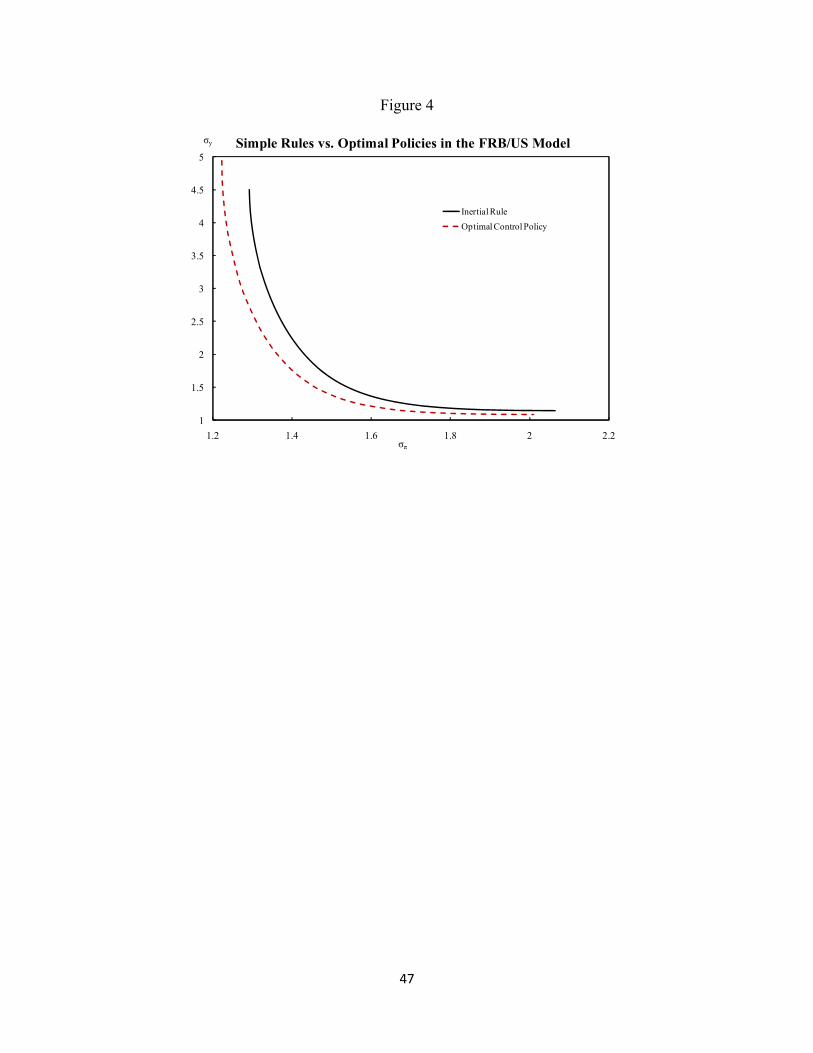
47  

Figure 4

1

1.5

2

2.5

3

3.5

4

4.5

5

1.2 1.4 1.6 1.8 2 2.2

Inertial Rule

Optimal Control Policy

Simple Rules vs. Optimal Policies in the FRB/US Model

σπ

σy

48  

Figure 5

0

50

100

150

200

0 0.3 0.6 0.9 1.2 1.5

Coefficient on Lagged Interest Rate (ρ)%ΔL

Woodford

Fuhrer

Rudebusch-Svensson

0

50

100

150

200

0 1 2 3 4

Coefficient on Inflation Rate (α)%ΔL

0

50

100

150

200

0 1 2 3

Coefficient on Output Gap (β)%ΔL

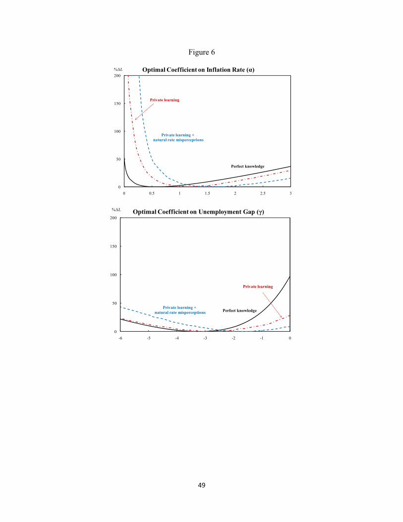
49  

Figure 6

 

 

 

0

50

100

150

200

0 0.5 1 1.5 2 2.5 3

Optimal Coefficient on Inflation Rate (α)

Perfect knowledge

Private learning

Private learning +natural rate misperceprions

%ΔL

0

50

100

150

200

-6 -5 -4 -3 -2 -1 0

Optimal Coefficient on Unemployment Gap (γ)

Perfect knowledge

Private learning

Private learning + natural rate misperceptions

%ΔL

50  

Figure 7

6

8

10

12

14

16

18

0 0.005 0.01 0.015 0.02 0.025 0.03

Robustness to Learning

κ

L

Modified OptimumControl Policy

Optimum ControlPolicy

Inertial RuleDifference Rule