simple beginning 3d openfoam...

Simple beginning 3D OpenFOAM Tutorial

Eng. Sebastian Rodriguez

www.libremechanics.com

Background. 1

Case definition. 1

3D modeling. 2

Units. 4

Physical parameters. 4

Meshing. 6

Structuring the case folders. 7

Boundary conditions. 7

Solving the case. 9

Post processing. 9

Comparing. 10


Eng. Sebastian Rodriguez 1 www.libremechanics.com

Simple beginning 3D OpenFoam Tutorial

OpenFOAM (Open Source Field Operation and

Manipulation) it’s an Open Source Software project

claim to be one of the best CFD tools currently

available, principally be its constant development

and its highly technical structure, the fine

implementation of common solvers and the

possibility to edit and create equations and

mathematical cases make OpenFOAM useful tool

on researching. OpenFOAM is a C++ toolbox for

the development of customized numerical solvers,

and pre-/post-processing utilities for the solution of

continuum mechanics problems, including

computational fluid dynamics (CFD). The code is

released as free and open source software under

the GNU General Public License

It is obvious a first contact that OpenFoam have a

more complex structure that most CAE and even

OpenSource engineering programs that request

much more capabilities from the user in other to

solve even the most common set cases; this is way

OpenFOAM it’s considered a “tough” program to

learn and work with, mostly by the lack of SIMPLE

documentation.

“In common plastic analysis, deformations are

easily inferred, but de fluid computational

dynamics its governed by a wide group of less

known physics laws and variables that make

the results almost unpredictable by simple

observation”

There it’s, actually, a great amount of technical

documentation on the web for users and

developers but in some cases y relays on strong

previous mathematical knowledge. Currently a

great variety of tutorials and examples are

emerging from investigation and work groups

around the world to help new user to understand

the program.

As the user is probably aware by now, the document make a number of simplifying assumptions as the tutorial progressed, this is done in the interest of gaining a clearer understanding of these fundamental without getting bogged down in

special details and exceptions. By no means it hast the complete history of 3D fluid analysis handling on OpenFoam, it is much broader in scope that can be presented in a single document such as this, but it is sincerely hoped that this tutorial will enable one to do a better job on the definition, solution and study of this kind of analysis.

Background

This may be a simple OpenFoam tutorial but it’s

necessary for the user to have some previous

experience on meshing tools, FEA analysis, result

reading and computational skills.

There is a tool called SalomeMECA, a useful

multipurpose CAE tool which has the capability to

preprocessing OpenFOAM cases with more user

friendly interface. The installation and use of

SalomeMeca, even easy may complicated this

beginning tutorial, for that reason will not be used

for preparing the model, even so the user is

encourage to review this software for further

implementation.

Case introduction.

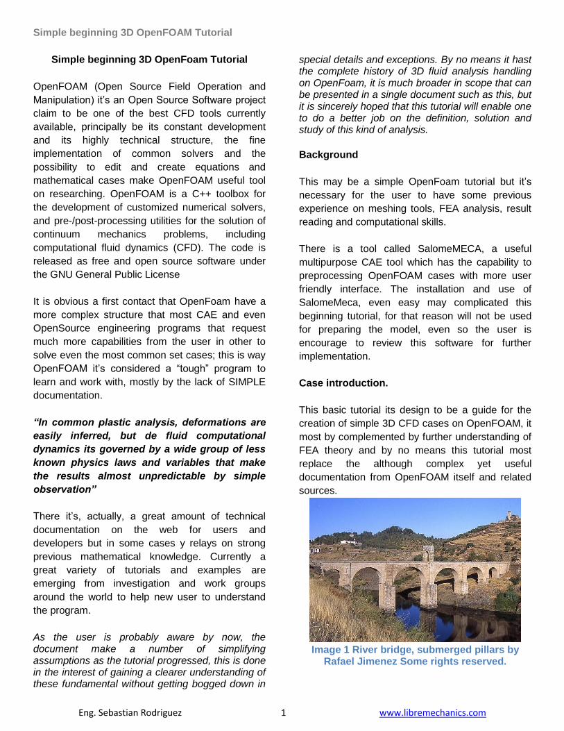
This basic tutorial its design to be a guide for the

creation of simple 3D CFD cases on OpenFOAM, it

most by complemented by further understanding of

FEA theory and by no means this tutorial most

replace the although complex yet useful

documentation from OpenFOAM itself and related

sources.

Image 1 River bridge, submerged pillars by

Rafael Jimenez Some rights reserved.



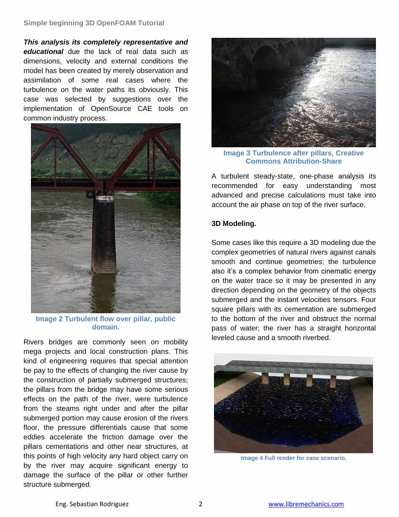
This analysis its completely representative and

educational due the lack of real data such as

dimensions, velocity and external conditions the

model has been created by merely observation and

assimilation of some real cases where the

turbulence on the water paths its obviously. This

case was selected by suggestions over the

implementation of OpenSource CAE tools on

common industry process.

Image 2 Turbulent flow over pillar, public

domain.

Rivers bridges are commonly seen on mobility

mega projects and local construction plans. This

kind of engineering requires that special attention

be pay to the effects of changing the river cause by

the construction of partially submerged structures;

the pillars from the bridge may have some serious

effects on the path of the river, were turbulence

from the steams right under and after the pillar

submerged portion may cause erosion of the rivers

floor, the pressure differentials cause that some

eddies accelerate the friction damage over the

pillars cementations and other near structures, at

this points of high velocity any hard object carry on

by the river may acquire significant energy to

damage the surface of the pillar or other further

structure submerged.

Image 3 Turbulence after pillars, Creative

Commons Attribution-Share

A turbulent steady-state, one-phase analysis its

recommended for easy understanding most

advanced and precise calculations must take into

account the air phase on top of the river surface.

3D Modeling.

Some cases like this require a 3D modeling due the

complex geometries of natural rivers against canals

smooth and continue geometries; the turbulence

also it’s a complex behavior from cinematic energy

on the water trace so it may be presented in any

direction depending on the geometry of the objects

submerged and the instant velocities tensors. Four

square pillars with its cementation are submerged

to the bottom of the river and obstruct the normal

pass of water; the river has a straight horizontal

leveled cause and a smooth riverbed.

Image 4 Full render for case scenario.



Image 5 Front render view of pillars.

Image 6 Side full render for case scenario.

Image 7 Side render view for pillars.

A classic no real 3D model was prepared for the

analysis which is not presentation or any real

structure or location, where the “worst case

scenario” was sought. An advise must be done for

the roughness of the model and the arrange of

pillars over the riverbed, in real cases the pillars are

not perfect squares and are not arranged like in the

model, but it this fictitious design should show

exactly way there is commonly rejected by

designers.

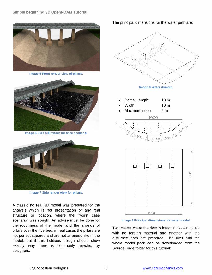
The principal dimensions for the water path are:

Image 8 Water domain.

Partial Length: 10 m

Width: 10 m

Maximum deep: 2 m

Image 9 Principal dimensions for water model.

Two cases where the river is intact in its own cause

with no foreign material and another with the

disturbed path are prepared. The river and the

whole model pack can be downloaded from the

SourceForge folder for this tutorial:



Units

http://www.openfoam.org/docs/user/basic-file-

format.php

Units on OpenFoam need to be set in order to be

accepted by the solver, the program makes an

early check for unit’s congruency and stops if

anything unusual is detected. In this case there is

no need for unit combinational scheme as other

FEA tool which makes easiest the reading of

results.

No. Property SI unit USCS unit

1 Mass kilogram

(kg)

pound-mass (lbm)

2 Length metre (m)

foot (ft)

3 Time second (s)

4 Temperature Kelvin

(K)

degree Rankine

(R)

5 Quantity kilogram-

mole (kgmol)

pound-mole

(lbmol)

6 Current ampere (A)

7 Luminous intensity

candela (cd)

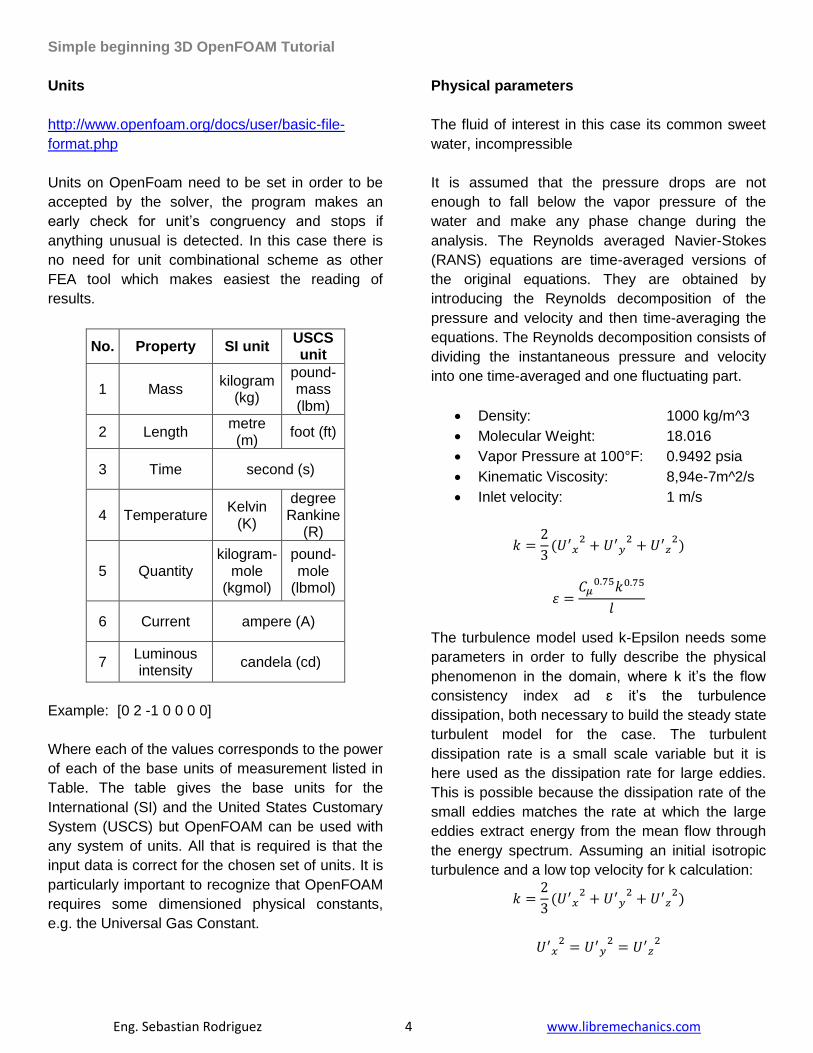
Example: [0 2 -1 0 0 0 0]

Where each of the values corresponds to the power

of each of the base units of measurement listed in

Table. The table gives the base units for the

International (SI) and the United States Customary

System (USCS) but OpenFOAM can be used with

any system of units. All that is required is that the

input data is correct for the chosen set of units. It is

particularly important to recognize that OpenFOAM

requires some dimensioned physical constants,

e.g. the Universal Gas Constant.

Physical parameters

The fluid of interest in this case its common sweet

water, incompressible

It is assumed that the pressure drops are not

enough to fall below the vapor pressure of the

water and make any phase change during the

analysis. The Reynolds averaged Navier-Stokes

(RANS) equations are time-averaged versions of

the original equations. They are obtained by

introducing the Reynolds decomposition of the

pressure and velocity and then time-averaging the

equations. The Reynolds decomposition consists of

dividing the instantaneous pressure and velocity

into one time-averaged and one fluctuating part.

Density: 1000 kg/m^3

Molecular Weight: 18.016

Vapor Pressure at 100°F: 0.9492 psia

Kinematic Viscosity: 8,94e-7m^2/s

Inlet velocity: 1 m/s

The turbulence model used k-Epsilon needs some

parameters in order to fully describe the physical

phenomenon in the domain, where k it’s the flow

consistency index ad ɛ it’s the turbulence

dissipation, both necessary to build the steady state

turbulent model for the case. The turbulent

dissipation rate is a small scale variable but it is

here used as the dissipation rate for large eddies.

This is possible because the dissipation rate of the

small eddies matches the rate at which the large

eddies extract energy from the mean flow through

the energy spectrum. Assuming an initial isotropic

turbulence and a low top velocity for k calculation:

http://www.openfoam.org/docs/user/basic-file-format.php

http://www.openfoam.org/docs/user/basic-file-format.php



The turbulence length scale , is a physical quantity

describing the size of the large energy-containing

eddies in a turbulent flow. The turbulent length

scale is often used to estimate the turbulent

properties on the inlets of a CFD simulation. Since

the turbulent length scale is a quantity which is

intuitively easy to relate to the physical size of the

problem it is easy to guess a reasonable value of

the turbulent length scale.

The turbulent length scale should normally not be

larger than the dimension of the problem, since that

would mean that the turbulent eddies are larger

than the problem size.

For This open channel flow the l dimension its

assumed to be:

Where the area and wet perimeter correspond to

the inlet velocity face of the water model.

Having the specific length and knowing is a

constant for this fluid k-epsilon case of 0.09 the

equation goes:

Commonly for achieving an specific grade of

turbulence some Reynolds number its specify to

determine an equivalent value of kinematic

viscosity, in this case the viscosity is already known

so the next calculation it’s just to check the

Reynolds number for the initial case:

| |

|

|

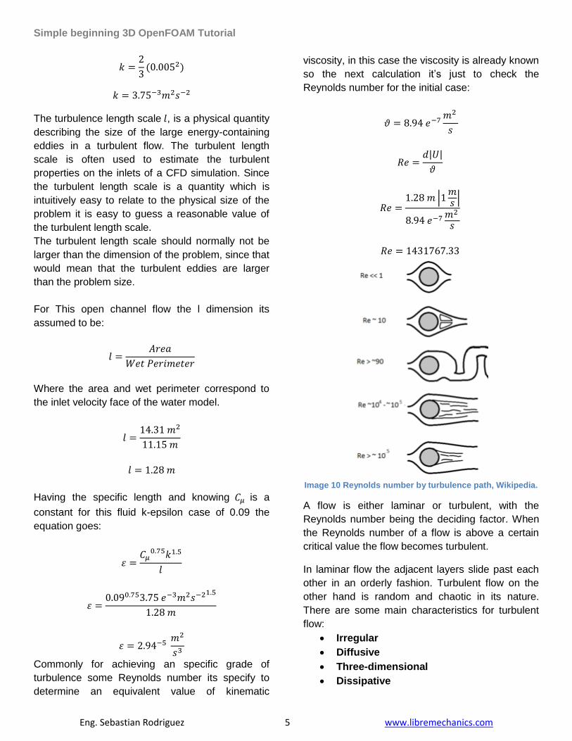
Image 10 Reynolds number by turbulence path, Wikipedia.

A flow is either laminar or turbulent, with the

Reynolds number being the deciding factor. When

the Reynolds number of a flow is above a certain

critical value the flow becomes turbulent.

In laminar flow the adjacent layers slide past each

other in an orderly fashion. Turbulent flow on the

other hand is random and chaotic in its nature.

There are some main characteristics for turbulent

flow:

Irregular

Diffusive

Three-dimensional

Dissipative



Meshing

Meshing for CFD analysis it’s always a challenge or

at least dong it thoroughly, 2D internal areas and

3D volumes must have a smooth distributed

element density, on contrast to plastic and elastic

FEA analysis where just a fine superficial and a

rough internal mesh its enough the CFD media

have a strong internal dependency for transient

conditions like velocity and pressure.

Even though OpenFOAM have a build in tool called

blockMesh for multi-block simple geometry

meshing, there is a need in CFD for multiple

meshing tools that cover a range of complexity of

meshing task. At one extreme, there is meshing

software that allows the user to define simple

geometries and mesh to those geometries. At the

other extreme, there is software that meshes to

highly complex CAD surfaces. In between, there is

room for one or two tools that generate optimal

meshes for moderately complex surfaces.

The user may choose its preferred meshing tool for

the geometry, in this case a simple NetGen mesh

will be used keeping in mind the recommendations

for this case; has to be noted that NetGen may be

not the best meshing tool for CFD analysis mainly

by the tetrahedral optimization process which is

recognized by, but it’s simple use and speed make

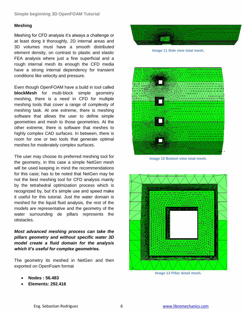
it useful for this tutorial. Just the water domain is

meshed for the liquid fluid analysis, the rest of the

models are representative and the geometry of the

water surrounding de pillars represents the

obstacles.

Most advanced meshing process can take the

pillars geometry and without specific water 3D

model create a fluid domain for the analysis

which it’s useful for complex geometries.

The geometry its meshed in NetGen and then

exported on OpenFoam format

Nodes : 56.483

Elements: 292.416

Image 11 Side view total mesh.

Image 12 Bottom view total mesh.

Image 13 Pillar detail mesh.



Structuring the case folders

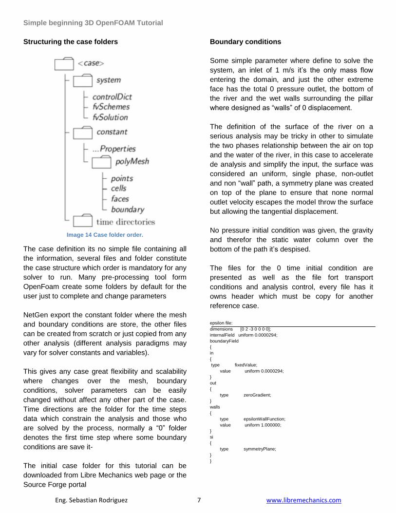
Image 14 Case folder order.

The case definition its no simple file containing all

the information, several files and folder constitute

the case structure which order is mandatory for any

solver to run. Many pre-processing tool form

OpenFoam create some folders by default for the

user just to complete and change parameters

NetGen export the constant folder where the mesh

and boundary conditions are store, the other files

can be created from scratch or just copied from any

other analysis (different analysis paradigms may

vary for solver constants and variables).

This gives any case great flexibility and scalability

where changes over the mesh, boundary

conditions, solver parameters can be easily

changed without affect any other part of the case.

Time directions are the folder for the time steps

data which constrain the analysis and those who

are solved by the process, normally a “0” folder

denotes the first time step where some boundary

conditions are save it-

The initial case folder for this tutorial can be

downloaded from Libre Mechanics web page or the

Source Forge portal

Boundary conditions

Some simple parameter where define to solve the

system, an inlet of 1 m/s it’s the only mass flow

entering the domain, and just the other extreme

face has the total 0 pressure outlet, the bottom of

the river and the wet walls surrounding the pillar

where designed as “walls” of 0 displacement.

The definition of the surface of the river on a

serious analysis may be tricky in other to simulate

the two phases relationship between the air on top

and the water of the river, in this case to accelerate

de analysis and simplify the input, the surface was

considered an uniform, single phase, non-outlet

and non “wall” path, a symmetry plane was created

on top of the plane to ensure that none normal

outlet velocity escapes the model throw the surface

but allowing the tangential displacement.

No pressure initial condition was given, the gravity

and therefor the static water column over the

bottom of the path it’s despised.

The files for the 0 time initial condition are

presented as well as the file fort transport

conditions and analysis control, every file has it

owns header which must be copy for another

reference case.

epsilon file:

dimensions [0 2 -3 0 0 0 0];

internalField uniform 0.0000294;

boundaryField

{

in

{

type fixedValue;

value uniform 0.0000294;

}

out

{

type zeroGradient;

}

walls

{

type epsilonWallFunction;


}

si

{

type symmetryPlane;

}

}



k file:

dimensions [0 2 -2 0 0 0 0];

internalField uniform 0.00375;

boundaryField

{

in

{

type fixedValue;

value uniform 0.1;

}

out

{

type zeroGradient;

}

walls

{

type kqRWallFunction;


}

si

{

type symmetryPlane;

}

}

P file:

dimensions [0 2 -2 0 0 0 0];

internalField uniform 0;

boundaryField

{

in

{

type zeroGradient;

}

out

{

type fixedValue;

value uniform 0;

}

walls

{

type zeroGradient;

}

si

{

type symmetryPlane;

}

}

U file:

dimensions [0 1 -1 0 0 0 0];

internalField uniform (0 0 0);

boundaryField

{

in

{

type fixedValue;

value uniform (1.000000 0.000000 0.0000);

}

out

{

type zeroGradient;

}

walls

{

type fixedValue;

value uniform (0. 0. 0.);

}

si

{

type symmetryPlane;

}

}

transportProperties file:

transportModel Newtonian;

nu nu [ 0 2 -1 0 0 0 0 ] 0.000000894;

CrossPowerLawCoeffs

{

nu0 nu0 [ 0 2 -1 0 0 0 0 ] 1e-06;

nuInf nuInf [ 0 2 -1 0 0 0 0 ] 1e-06;

m m [ 0 0 1 0 0 0 0 ] 1;

n n [ 0 0 0 0 0 0 0 ] 1;

}

BirdCarreauCoeffs

{

nu0 nu0 [ 0 2 -1 0 0 0 0 ] 1e-06;

nuInf nuInf [ 0 2 -1 0 0 0 0 ] 1e-06;

k k [ 0 0 1 0 0 0 0 ] 0;

n n [ 0 0 0 0 0 0 0 ] 1;

}

ControlDic for pillars model

application simpleFoam;

startFrom latestTime;

startTime 0;

stopAt endTime;

endTime 500;

deltaT 10;

writeControl timeStep;

writeInterval 1;

purgeWrite 0;

writeFormat ascii;

writePrecision 6;

writeCompression off;

timeFormat general;

timePrecision 6;

runTimeModifiable true;

ControlDic for clean model:

application simpleFoam;

startFrom latestTime;

startTime 0;

stopAt endTime;

endTime 300;

deltaT 10;

writeControl timeStep;

writeInterval 1;

purgeWrite 0;

writeFormat ascii;

writePrecision 6;

writeCompression off;

timeFormat general;

timePrecision 6;

runTimeModifiable true;

The files for the 0 step are similar for both cases,

the controlDict file most change in order to give the

solver the steps scheme need it to converge in the

equations resolution. The accurate formula to

define the step length and the dertaT interval its

given by the Courant number:

http://inside.mines.edu/~epoeter/583/13/discussion/

courant.htm

http://en.wikipedia.org/wiki/Courant%E2%80%93Fri

edrichs%E2%80%93Lewy_condition

http://inside.mines.edu/~epoeter/583/13/discussion/courant.htm

http://inside.mines.edu/~epoeter/583/13/discussion/courant.htm

http://en.wikipedia.org/wiki/Courant%E2%80%93Friedrichs%E2%80%93Lewy_condition

http://en.wikipedia.org/wiki/Courant%E2%80%93Friedrichs%E2%80%93Lewy_condition



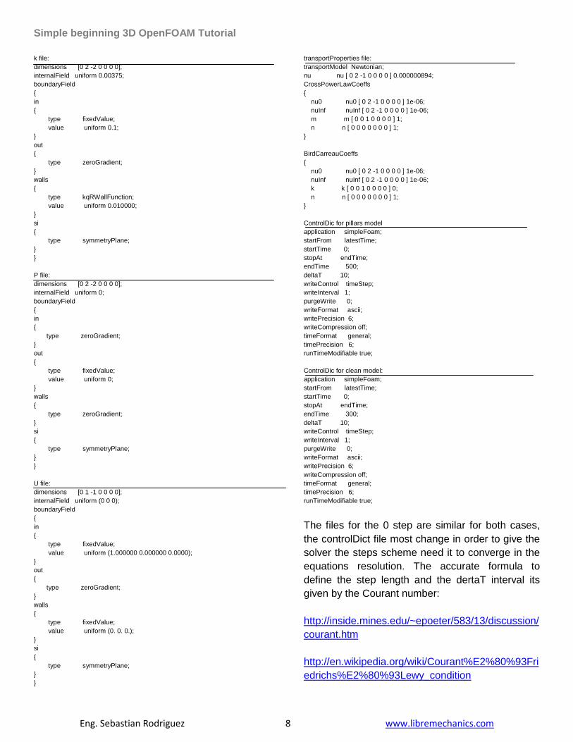
Solving the case:

The size of the mesh and the steps the solver must

run, request the use of multiple cores for the

OpenFOAM solver to decrease the solving time.

./cleanAll.sh

This command cleans the working folder

from previous results.

mpirun -np 4 simpleFoam -parallel

Image 15 Multi core use for the OpenFoam solver.

The solver creates the time step folders on the

main work case folder, each step contains the

velocity and pressure values, this structure allows

to exchange result data from case to case.

Its recommendable to pay attention to the console

output to capture any warning or error from the

solver messages.

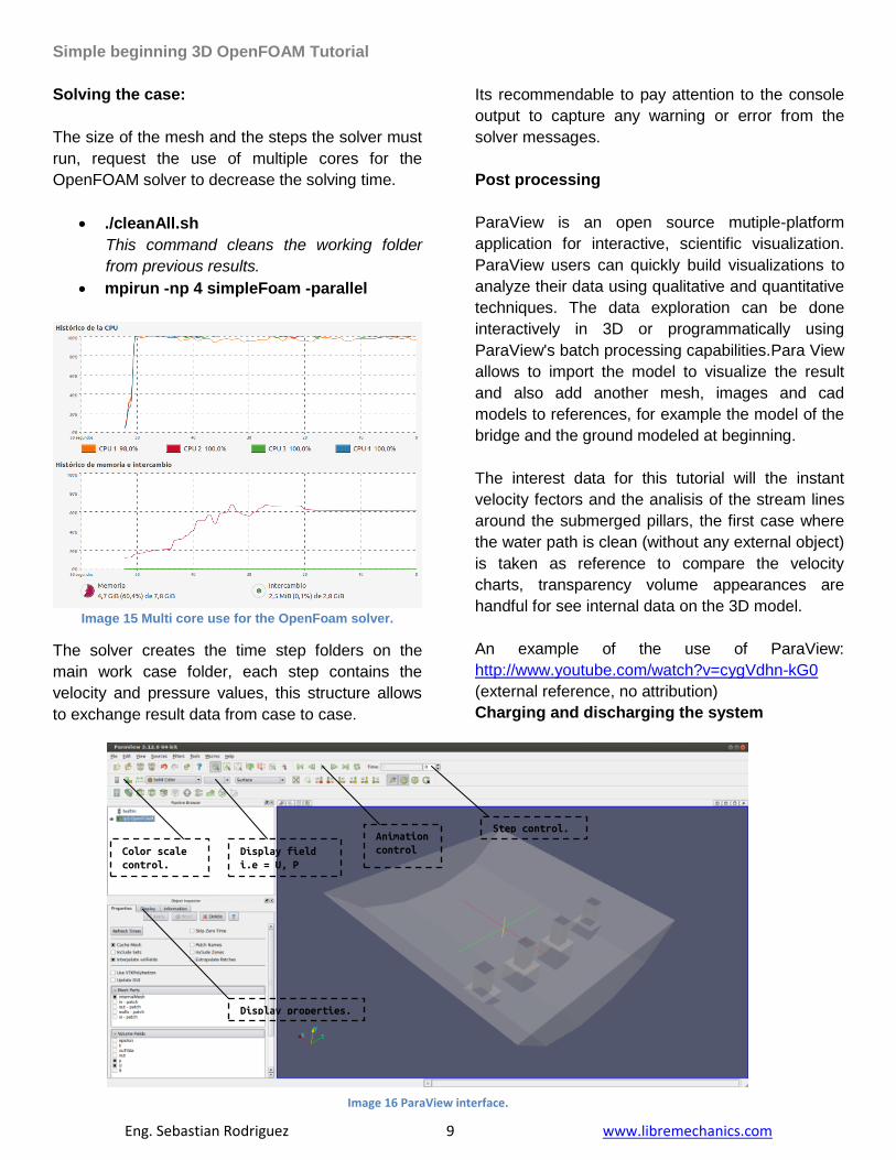
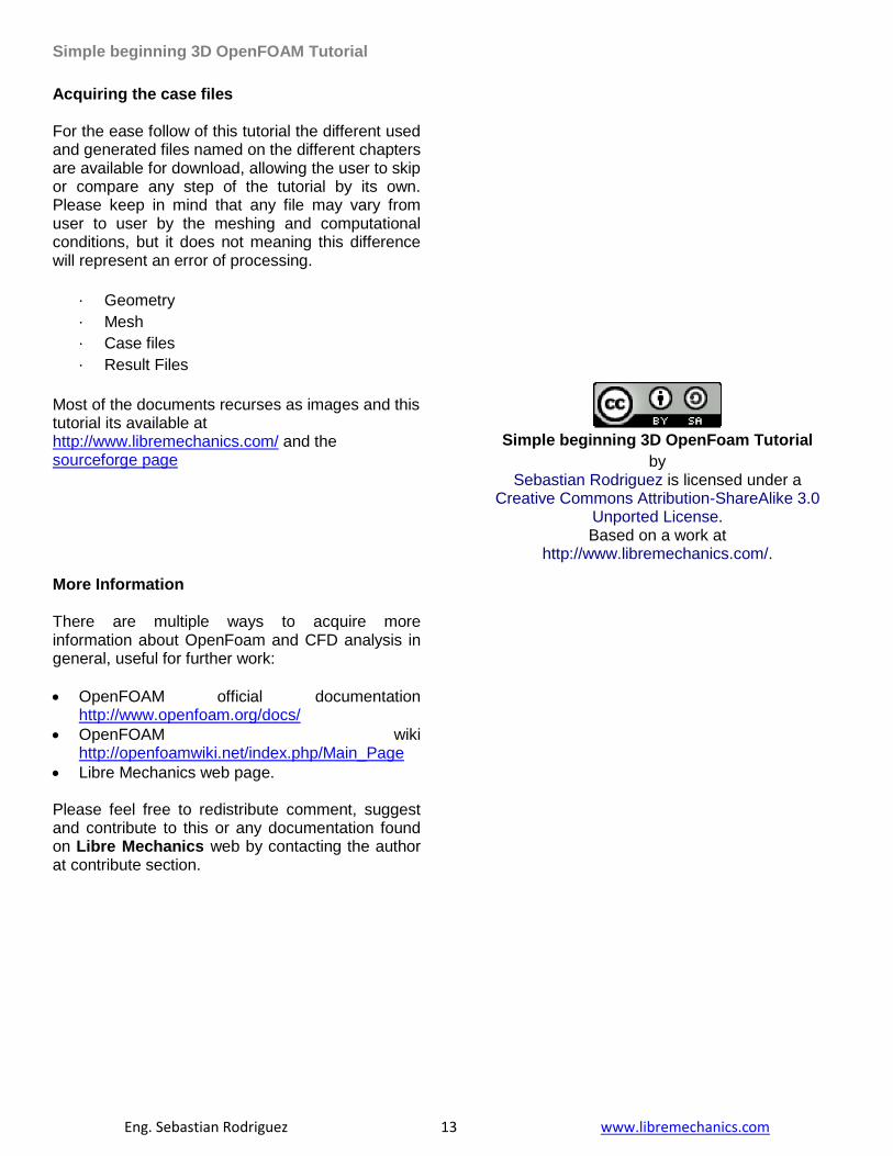
Post processing

ParaView is an open source mutiple-platform

application for interactive, scientific visualization.

ParaView users can quickly build visualizations to

analyze their data using qualitative and quantitative

techniques. The data exploration can be done

interactively in 3D or programmatically using

ParaView's batch processing capabilities.Para View

allows to import the model to visualize the result

and also add another mesh, images and cad

models to references, for example the model of the

bridge and the ground modeled at beginning.

The interest data for this tutorial will the instant

velocity fectors and the analisis of the stream lines

around the submerged pillars, the first case where

the water path is clean (without any external object)

is taken as reference to compare the velocity

charts, transparency volume appearances are

handful for see internal data on the 3D model.

An example of the use of ParaView:

http://www.youtube.com/watch?v=cygVdhn-kG0

(external reference, no attribution)

Charging and discharging the system

Image 16 ParaView interface.

Display properties.

Color scale

control.

Display field

i.e = U, P

Step control. Animation

control

http://www.youtube.com/watch?v=cygVdhn-kG0



Some result may seem inappropriate for the steady

state fluid analysis of the case, this respond to the

charging which the inlet velocity condition takes to

fully overload the domain and reached the outlet,

some time-steps must be overlooked to ensure the

continuity of the system.

Comparing the two cases

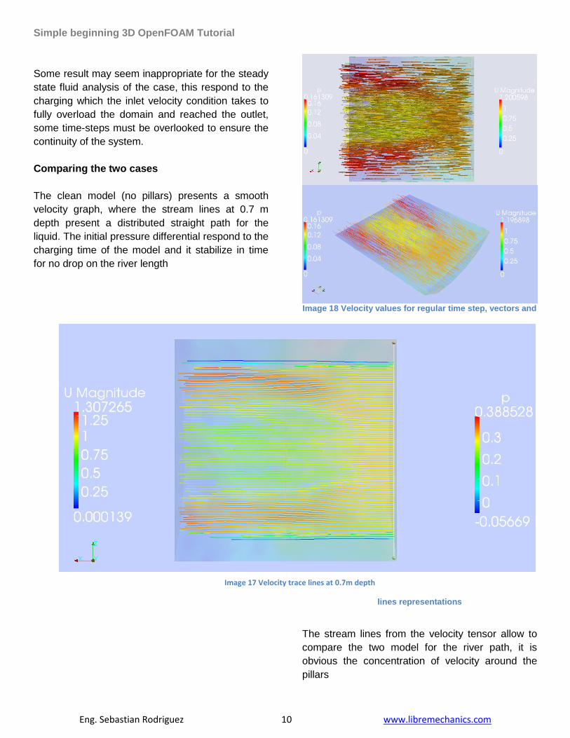
The clean model (no pillars) presents a smooth

velocity graph, where the stream lines at 0.7 m

depth present a distributed straight path for the

liquid. The initial pressure differential respond to the

charging time of the model and it stabilize in time

for no drop on the river length

Image 18 Velocity values for regular time step, vectors and

lines representations

The stream lines from the velocity tensor allow to

compare the two model for the river path, it is

obvious the concentration of velocity around the

pillars

Image 17 Velocity trace lines at 0.7m depth



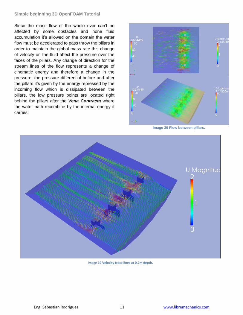
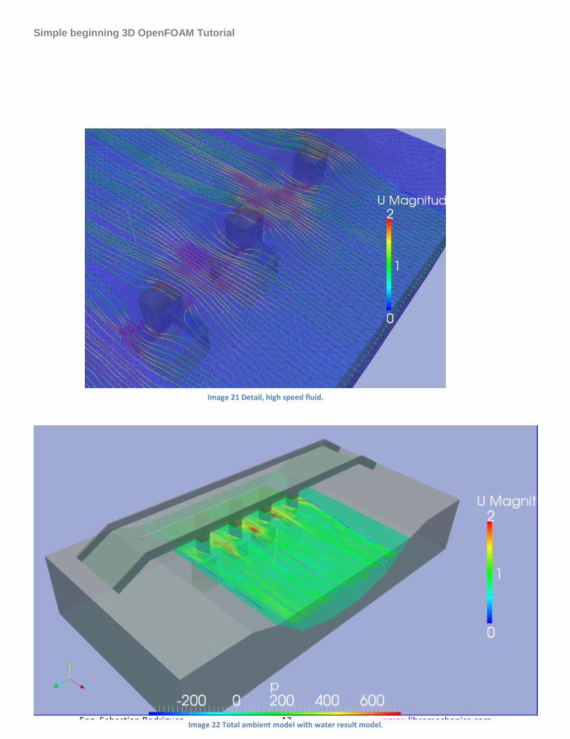
Since the mass flow of the whole river can’t be

affected by some obstacles and none fluid

accumulation it’s allowed on the domain the water

flow must be accelerated to pass throw the pillars in

order to maintain the global mass rate this change

of velocity on the fluid affect the pressure over the

faces of the pillars. Any change of direction for the

stream lines of the flow represents a change of

cinematic energy and therefore a change in the

pressure, the pressure differential before and after

the pillars it’s given by the energy repressed by the

incoming flow which is dissipated between the

pillars, the low pressure points are located right

behind the pillars after the Vena Contracta where

the water path recombine by the internal energy it

carries.

Image 20 Flow between pillars.

Image 19 Velocity trace lines at 0.7m depth.



Image 21 Detail, high speed fluid.

Image 22 Total ambient model with water result model.



Acquiring the case files For the ease follow of this tutorial the different used and generated files named on the different chapters are available for download, allowing the user to skip or compare any step of the tutorial by its own. Please keep in mind that any file may vary from user to user by the meshing and computational conditions, but it does not meaning this difference will represent an error of processing.

· Geometry

· Mesh

· Case files

· Result Files

Most of the documents recurses as images and this tutorial its available at http://www.libremechanics.com/ and the sourceforge page

More Information There are multiple ways to acquire more information about OpenFoam and CFD analysis in general, useful for further work:

OpenFOAM official documentation http://www.openfoam.org/docs/

OpenFOAM wiki http://openfoamwiki.net/index.php/Main_Page

Libre Mechanics web page. Please feel free to redistribute comment, suggest and contribute to this or any documentation found on Libre Mechanics web by contacting the author at contribute section.

Simple beginning 3D OpenFoam Tutorial

by Sebastian Rodriguez is licensed under a

Creative Commons Attribution-ShareAlike 3.0 Unported License. Based on a work at

http://www.libremechanics.com/.

http://www.libremechanics.com/

http://sourceforge.net/projects/libremechanics/

http://www.openfoam.org/docs/

http://openfoamwiki.net/index.php/Main_Page

simple beginning 3d openfoam...

Documents