simulating propagation of decoupled elastic waves … propagation of decoupled elastic waves using...

Simulating propagation of decoupled elastic waves

using low-rank approximate mixed-domain integral

operators for anisotropic mediaa

aPublished in Geophysics, 81, no. 2, T63-T77, (2016)

Jiubing Cheng1, Tariq Alkhalifah2, Zedong Wu3, Peng Zou4 and Chenlong Wang5

ABSTRACT

In elastic imaging, the extrapolated vector fields are decoupled into pure wavemodes, such that the imaging condition produces interpretable images. Conven-tionally, mode decoupling in anisotropic media is costly as the operators involvedare dependent on the velocity, and thus are not stationary. We develop an effi-cient pseudo-spectral approach to directly extrapolate the decoupled elastic wavesusing low-rank approximate mixed-domain integral operators on the basis of theelastic displacement wave equation. We apply k-space adjustment to the pseudo-spectral solution to allow for a relatively large extrapolation time-step. Thelow-rank approximation is, thus, applied to the spectral operators that simulta-neously extrapolate and decompose the elastic wavefields. Synthetic examples ontransversely isotropic and orthorhombic models show that, our approach has thepotential to efficiently and accurately simulate the propagations of the decou-pled quasi-P and quasi-S modes as well as the total wavefields, for elastic wavemodeling, imaging and inversion.

INTRODUCTION

Multicomponent seismic data are increasingly acquired on land and at the oceanbottom in an attempt to better understand the geological structure and characterizeoil and gas reservoirs. Seismic modeling, reverse-time migration (RTM), and full-waveform inversion (FWI) in areas with complex geology all require high-accuracynumerical algorithms for time extrapolation of waves. Because seismic waves propa-gate through the earth as a superposition of P- and S-wave modes, an elastic waveequation is usually more accurate for wavefield extrapolation than an acoustic waveequation. Wave mode decoupling can not only help elastic imaging to produce physi-cally interpretable images, which characterize reflectivities of various reflection types(Wapenaar et al., 1987; Dellinger and Etgen, 1990; Yan and Sava, 2008), but alsoprovide more opportunity to mitigate the parameter trade-offs in elastic waveforminversion (Wang and Cheng, 2015).

Cheng et al. 2Propagate decoupled anisotropic elastic waves

For isotropic media, far-field P and S waves can be separated by taking the diver-gence and curl in the extrapolated elastic wavefields (Aki and Richards, 1980; Sunand McMechan, 2001). Alternatively, Ma and Zhu (2003) and Zhang et al. (2007)extrapolated vector P and S modes separately in an elastic wavefield by decomposingthe wave equation into P- and S-wave components. In the meantime, decouplingof wave modes yields familiar scalar wave equations for P and S modes (Aki andRichards, 1980). In anisotropic media, one cannot, so simply, derive explicit single-mode time-space-domain differential wave equations. Generally, P and S modes donot respectively polarize parallel and perpendicular to the wave vectors, and thus arecalled quasi-P (qP) and quasi-S (qS) waves. They cannot be fully decoupled withdivergence and curl operations (Dellinger and Etgen, 1990).

Anisotropic wave propagation can be formally decoupled in the wavenumber-domain to yield single-mode pseudo-differential equations (Liu et al., 2009). Un-fortunately, these equations in time-space domain cannot be solved with traditionalnumerical schemes unless further approximation to the dispersion relation or phasevelocity is applied (Etgen and Brandsberg-Dahl, 2009; Chu et al., 2011; Fowler andKing, 2011; Zhan et al., 2012; Song and Alkhalifah, 2013; Wu and Alkhalifah, 2014;Du et al., 2014). To avoid solving the pseudo-differential equation, Xu and Zhou(2014) proposed a nonlinear wave equation for pseudoacoustic qP-wave with an aux-iliary scalar operator depending on the material parameters and the phase directionof the propagation at each spatial location. All these efforts are restricted to pure-mode scalar waves and do not honor the elastic effects such as mode conversion.Cheng and Kang (2014) and Kang and Cheng (2012) have proposed approaches topropagate the partially decoupled wave modes using the so-called pseudo-pure-modewave equations, and then obtain completely decoupled qP or qS waves by correct-ing the polarization deviation of the pseudo-pure-mode wavefields. Their approacheshonor the kinematics of all wave modes but may distort the reflection/transmissioncoefficients if high contrasts exist in the velocity fields.

Alternatively, many have developed approaches to decouple qP- and qS-wavemodes from the extrapolated elastic wavefields. Dellinger and Etgen (1990) general-ized the divergence and curl operations to anisotropic media by constructing separa-tors as polarization projection in the wavenumber-domain. To tackle heterogeneity,these mode separators were rewritten by Yan and Sava (2009) as nonstationary spatialfilters determined by the local polarization directions. Zhang and McMechan (2010)proposed a wavefield decomposition method to separate elastic wavefields into vectorqP- and qS-wave fields for vertically transverse isotropic (VTI) media. Accordingly,Cheng and Fomel (2014) proposed fast mixed-domain algorithms for mode separationand vector decomposition in heterogeneous anisotropic media by applying low-rankapproximation to the involved Fourier integral operators (FIOs) of the general form.

The motivation of this study is to develop an efficient approach to propagate anddecouple the elastic waves for general anisotropic media. The primary strategy isto merge the numerical solutions for time extrapolation and vector decompositioninto a unified Fourier integral framework and speed up the solutions using the low-


rank approximation. This paper is organized as follows. We first demonstrate apseudo-spectral solution to extrapolate the elastic displacement wavefields in time-domain. Then we propose to merge the spectral operations for time extrapolationinto the integral framework for vector decomposition of the wave modes. Applyinglow-rank approximations to the involved mixed-domain matrices, we obtain an effi-cient algorithm for simultaneous propagating and decoupling the elastic wavefields.We demonstrate the validity of the proposed method using 2-D and 3-D syntheticexamples on the transversely isotropic (TI) and orthorhombic models with increasingcomplexity.

PROPAGATING COUPLED ELASTIC WAVEFIELDS

Following Carcione (2007), we denote the spatial variables x, y and z of a right-handCartesian system by the indices i, j, . . . = 1, 2 and 3, respectively, the position vectorby x, a partial derivative with respect to a variable xi with ∂i, and the first and secondtime derivatives with ∂t and ∂tt. Matrix transposition is denoted by the superscript“T”. We also denote

√−1 by i, the scalar and matrix products by the symbol “ · ”,

the dyadic product by the symbol “⊗ ”. The Einstein convention of repeated indicesis assumed unless otherwise specified.

Pseudo-spectral solution of the elastic wave equation

Wave propagation in general anisotropic elastic media is governed by the linearizedmomentum balance law and a linear constitutive relation between the stress andstrain tensors. These governing equations can be combined to write the displacementformalism as,

ρ∂2ttu = 5·[C · (5T · u)] + f , (1)

with u = (ux, uy, uz)T represents the vector wavefields, f is the body force vector perunit volume, C is the 6 × 6 elasticity matrix representing the stiffness tensor withthe Voigt’s menu, and the spatial differential operator 5 has the following matrixrepresentation:

5 =

∂x 0 0 0 ∂z ∂y

0 ∂y 0 ∂z 0 ∂x

0 0 ∂z ∂y ∂x 0

. (2)

The pseudo-spectral method calculates the spatial derivatives using the fast Fouriertransform (FFT), while approximating the temporal derivative with a finite-difference.Neglecting the source term, equation 1 is rewritten in the spatial Fourier-domain fora homogeneous medium as,

∂2ttu + Γu = 0, (3)

in which u is the wavefields in the wavenumber-domain, k = (kx, ky, kz) is thewavenumber vector, and Γ = 1/ρL · C · LT represents the 3 × 3 density normalized


Christoffel matrix with the wavenumber-domain counterpart of the space differentialoperator (removing the imaginary unit i) satisfies,

L =

kx 0 0 0 kz ky

0 ky 0 kz 0 kx

0 0 kz ky kx 0

. (4)

To calculate the 2nd-order temporal derivatives, we use the standard leapfrogscheme, i.e.,

∂2ttu

(n)i =

u(n+1)i − 2u

(n)i + u

(n−1)i

∆t2, (5)

in which ∆t = tn+1 − tn is the time-step. For constant density homogeneous media,applying the two-step time-marching scheme leads to the pseudo-spectral formula:

∂2ttu

(n) = Ψu(n), (6)

with the spectral operator defined with the following kernel:

Ψ := (2π)−3

∫ ∫Γ(k)eik·(x−y)dydk. (7)

Phase terms in the integral operator can be absorbed into forward and inverse Fouriertransforms. This implies that the wavefields are first transformed into wavenumber-domain using forward FFTs, then multiplied with the corresponding components ofthe Christoffel matrix, and finally transformed back into space-domain using inverseFFTs. For locally smooth media, we use a spatially varying Christoffel matrix totackle the heterogeneity, i.e.,

Ψ := (2π)−3

∫ ∫Γ(x,k)eik·(x−y)dydk. (8)

The extended formation of this pseudo-spectral elastic wave propagator is shown inAppendix B. Spectral methods are charaterized by the use of Fourier basis functionsto describe the field variables and have the advantages over finite-difference schemesthat the mesh requirements are more relaxed (Kosloff et al., 1989; Liu and Li, 2000).

Adjustment to the pseudo-spectral solution

Generally, the two-step time-marching pseudo-spectral solution is limited to a smalltime-step, as larger time-steps lead to numerical dispersion and stability issues. Atmore computational costs, high-order finite-difference (Dablain, 1986) can be appliedto address this difficulty. As an alternative to second-order temporal differencing,a time integration technique based on rapid expansion method (REM) can providehigher accuracy with less computational efforts (Kosloff et al., 1989). As Du et al.(2014) demonstrated, one-step time marching schemes (Zhang and Zhang, 2009; Sun


and Fomel, 2013), especially using optimized polynomial expansion, usually give moreaccurate approximations to heterogeneous extrapolators for larger time-steps. In thissection, we discuss a strategy to extend the time-step for the previous two-step time-marching pseudo-spectral scheme according to the eigenvalue decomposition of theChristoffel matrix.

Since the Christoffel matrix is symmetric positive definite, it has a unique eigen-decomposition of the form:

Γ =3∑

i=1

λ2i ai ⊗ ai, (9)

where λ2i ’s are the eigenvalues and ai’s are the eigenvectors of Γ, with ai · aj = δij.

The three eigenvalues correspond to phase velocities of the three wave modes withλi = vik (in which k = |k|, and vi represents the phase velocity) representing thecircular frequency, and the corresponding eigenvector ai = (aix, aiy, aiz) representsthe normalized polarization vector for the given mode. An alternative form of theabove decomposition yields:

Γ = QΛQT , (10)

with

Λ =

λ21 0 0

0 λ22 0

0 0 λ23

, (11)

Q =

a1x a2x a3x

a1y a2y a3y

a1z a2z a3z

. (12)

Note Q is an orthogonal matrix, i.e., Q−1 = QT .

The eigenvalues represent the frequencies and satisfy the condition given by,

λi = vik ≤ 2πfmax, (13)

in which fmax is the maximum frequency of the source. Therefore, we suggest to filterout the high-wavenumber components in the wavefields beyond 2πfmax/vmin (vmin isthe minimum phase velocity in the computational model) caused by the numericalerrors to enhance numerical stability.

According to above eigen-decomposition, we apply the k-space adjustment to ourpseudo-spectral scheme by modifying the eigenvalues of Christoffel matrix for theanisotropic elastic wave equation (see Appendix C), i.e.,

Λ =

λ21sinc

2(λ1∆t/2) 0 00 λ2

2sinc2(λ2∆t/2) 0

0 0 λ23sinc

2(λ3∆t/2)

. (14)

Thus this adjustment inserts a modified Christoffel matrix, i.e., Γ = QΛQT , into theoriginal pseudo-spectral formula on the basis of equations 6 and 8. Note that the


k-space adjustment to the pseudo-spectral solution has been widely used in acousticand ultrasound (Bojarski, 1982; Tabei et al., 2002) and elastic isotropic wavefieldsimulation (Liu, 1995; Firouzi et al., 2012).

PROPAGATING DECOUPLED ELASTIC WAVEFIELDS

Above pseudo-spectral operators propagate the elastic wavefields as a superpositionof qP- and qS-wave modes. To obtain physically interpretable results for seismicimaging and waveform inversion, wave mode decoupling is required during wavefieldextrapolation. The key concept of mode decoupling is based on polarization. Ina general anisotropic medium, the qP and qS modes do not polarize parallel andperpendicular to the wave vectors. Moreover, unlike the well-behaved qP mode, thetwo qS modes do not consistently polarize as a function of the propagation direction(or wavenumber) and thus cannot be designated as SV and SH waves, except inisotropic and TI media (Winterstein, 1990; Crampin, 1991). Even for a TI medium,it is a challenge to find the right solution of the shear singularity problem and obtaintwo completely separated S-modes with correct amplitudes (Yan and Sava, 2011;Cheng and Fomel, 2014). Therefore, we restrict to extrapolate the decoupled qP- andqS- wave modes in this paper.

Vector decomposition of the elastic wave modes

According to Zhang and McMechan (2010), one can decompose qP and qS modes inthe elastic wavefields for a homogeneous anisotropic medium using:

u(m)i (k) = d

(m)ij (k)uj(k), (15)

where m = {qP, qS}, i, j = {x, y, z}, and the decomposition operators satisfy:

d(qP )xx (k) = a2

x(k),

d(qP )yy (k) = a2

y(k),

d(qP )zz (k) = a2

z(k),

d(qP )xy (k) = ax(k)ay(k),

d(qP )xz (k) = ax(k)az(k),

d(qP )yz (k) = ay(k)az(k),

(16)

andd

(qS)xx (k) = a2

y(k) + a2z(k),

d(qS)yy (k) = a2

x(k) + a2z(k),

d(qS)zz (k) = a2

x(k) + a2yk),

d(qS)xy (k) = −ax(k)ay(k),

d(qS)xz (k) = −ax(k)az(k),

d(qS)yz (k) = −ay(k)az(k),

(17)


in which ax(k), ay(k) and az(k) represent the x-, y- and z-components of the nor-malized polarization vector of qP-wave.

As demonstrated by Cheng and Fomel (2014), one can decompose the wave modesin a heterogeneous anisotropic medium using the following mixed-domain integraloperations:

u(m)x (x) =

∫eikxd

(m)xx (x,k)ux(k) dk +

∫eikxd

(m)xy (x,k)uy(k) dk

+∫eikxd

(m)xz (x,k)uz(k) dk,

u(m)y (x) =

∫eikxd

(m)xy (x,k)ux(k) dk +

∫eikxd

(m)yy (x,k)uy(k) dk

+∫eikxd

(m)yz (x,k)uz(k) dk,

u(m)z (x) =

∫eikxd

(m)xz (x,k)ux(k) dk +

∫eikxd

(m)yz (x,k)uy(k) dk

+∫eikxd

(m)zz (x,k)uz(k) dk.

(18)

Extrapolating the decoupled elastic waves

For heterogeneous anisotropic media, the wavefield propagator (equation 6) and thevector decomposition operators (equation 18) are both in the general form of FIOs.Naturally, we merge them to derive a new mixed-domain integral solution for extrap-olating the decoupled elastic wavefields:

u(m)x (x, t+ ∆t) = −u(m)

x (x, t−∆t) +∫eikxw(m)

xx (x,k)ux(k, t) dk+

∫eikxw(m)

xy (x,k)uy(k, t) dk +∫eikxw(m)

xz (x,k)uz(k, t) dk,

u(m)y (x, t+ ∆t) = −u(m)

y (x, t−∆t) +∫eikxw(m)

yx (x,k)ux(k, t) dk+

∫eikxw(m)

yy (x,k)uy(k, t) dk +∫eikxw(m)

yz (x,k)uz(k, t) dk,

u(m)z (x, t+ ∆t) = −u(m)

z (x, t−∆t) +∫eikxw(m)

zx (x,k)ux(k, t) dk+

∫eikxw(m)

zy (x,k)uy(k, t) dk +∫eikxw(m)

zz (x,k)uz(k, t) dk,(19)

with the propagation matrices for the decoupled wave modes given as

w(m)ij (x,k) = d

(m)ki (x,k)wkj(x,k), (20)

in which wkj(x,k) is defined by the spatially varying Christoffel matrix and the lengthof time-step, namely

wkk(x,k) = 2−∆t2Γkk(x,k),wkj(x,k) = −∆t2Γkj(x,k).

(21)

The extended formulation of equation 20 is given in Appendix B. Note the symmetryproperties exist: d

(m)ki = d

(m)ik and wkj = wjk, and the modified Christoffel matrix will

be used if the k-space adjustment is applied for the pseudo-spectral solutions.

To drive the time extrapolation of the decomposed wavefields using equation 19,we must update the total elastic wavefields by superposing qP- and qS-waves at eachtime-step using

ux(x) = u(qP )x (x) + u

(qS)x (x),

uy(x) = u(qP )y (x) + u

(qS)y (x),

uz(x) = u(qP )z (x) + u

(qS)z (x).

(22)


Thus equations 19 to 22 compose the spectral-like operators to simultaneously extrap-olate and decouple the elastic wavefields for 3D anisotropic media. The computationcomplexity of the straightforward implementation of the integral operators in equa-tions 8 and 19 is O(N2

x), which is prohibitively expensive when the size of model Nx

is large.

To tackle strong heterogeneity due to fast varying stiffness coefficients, we suggestto split the displacement equation into the displacement-stress equation and thensolve it using the staggered-grid pseudo-spectral scheme (Ozdenvar and McMechan,1996; Carcione, 1999; Bale, 2003). Note when using staggered grids, the operators toextrapolate the decoupled wave modes must be modified in order to account for theshifts in medium properties and fields variables. We will investigate this issue in thefuture work.

FAST ALGORITHM USING LOW-RANKDECOMPOSITION

As proposed by Cheng and Fomel (2014), low-rank decomposition of the mixed-domain matrix d(x,k) in equation 18 yields very efficient algorithm for mode de-coupling in heterogeneous anisotropic media. We find that the same strategy worksfor numerical implementations of above pseudo-spectral operators for elastic wavepropagation.

For example, the mixed-domain matrix, i.e., w(x,k) or w(x,k) in the FIOs, canbe approximated by the following separated representation (Fomel et al., 2013):

W (x,k) ≈∑M

m=1

∑Nn=1B(x,km)AmnC(xn,k), (23)

in which B(x,km) is a mixed-domain matrix with reduced wavenumber dimension M ,C(xn,k) is a mixed-domain matrix with reduced spatial dimension N , Amn is a M×Nmatrix with N and M representing the rank of this decomposition. Physically, a sep-arable low-rank approximation amounts to selecting a set of N (N � Nx) represen-tative spatial locations and M (M � Nx) representative wavenumbers. Constructionof the separated representation follows the method of Engquist and Ying (2009). Theranks M and N are dependent on the complexities (heterogeneity and anisotropy)of the medium and the estimate of the approximation accuracy to the mixed-domainmatrices (In the numerical examples, we aim for the relative single-precision accuracyof 10−6). More explainations on low-rank decomposition is available in Fomel et al.(2013) and Cheng and Fomel (2014). As we observe, the ranks are generally verysmall for our applications. For homogeneous media, the ranks naturally reduce to 1.If there is heterogeneity, the ranks increase to 2 for isotropic media but exceed 2 foranisotropic media. The k-space adjustment may slightly increase the ranks for theheterogeneous media.


Thus the above low-rank approximation speeds up computation of the FIOs since∫eikxW (x,k)uj(k) dk

≈∑M

m=1B(x,km)(∑N

n=1Amn

(∫eikxC(xn,k)uj(k) dk

)).

(24)

Evaluation of the last formula is effectively equivalent to applying N inverse FFTseach time-step. Accordingly, the computation complexity reduces to O(NNx logNx).In multiple-core implementations, the matrix operations in equation 24 are easy toparallelize.

EXAMPLES

We will first demonstrate the proposed approach on two-layer TI and orthorhombicmodels, and then on the complex SEG Hess VTI and BP 2007 TTI models, repec-tively.

2D two-layer VTI/TTI model

The first example is on a 2D two-layer model, in which the first layer is a VTI mediumwith vp0 = 2500m/s, vs0 = 1200m/s, ε = 0.2, and δ = −0.2, and the second layer isa tilted TI (TTI) medium with vp0 = 3600m/s, vs0 = 1800m/s, ε = 0.2, δ = 0.1 andθ = 30◦. A point source is placed at the center of this model. Firstly, we compare thesynthetic elastic wavefields by solving the elastic displacement wave equation usingthe 10th-order explicit finite-difference (FD) and low-rank pseudo-spectral schemes(with or without the k-space adjustment), respectively. Figure 1 shows the wavefieldsnapshots at the time of 0.3 s using the spatial sampling ∆x = ∆z = 5m and time-step ∆t = 0.5ms. Only the low-rank pseudo-spectral solutions with the k-spaceadjustment are displayed because the three schemes produce very similar results.The vertical slices through the z-components of the elastic wavefields show littledifferences among them (Figure 2). For the low-rank pseudo-spectral scheme, theranks are all 2 for the decomposition of the mixed-domain matrices wxx, wzz and wxz

in equation 21, and the k-space adjustment doesn’t change the ranks. It takes CPUtime of 0.20, 0.23 and 0.23 seconds for them to finish the wavefield extrapolation ofone time-step. Additional 4.3 and 8.2 seconds have been used to finish the low-rankdecomposition of the involved mixed-domain matrices before wavefield extrapolation.We observe the FD scheme unstable if the time-step is increased to 1.0 ms and thelow-rank pseudo-spectral scheme unstable if the time-step is increased to 2.0 ms (withunchanged spatial sampling). However, the low-rank pseudo-spectral solution usingthe k-space adjustment produces acceptable results even the time-step is increasedto 3.0 ms and the maximum time exceeds 3 s. Figure 3 and Figure 4 compare thewavefield snapshots and the vertical slices at the time of 0.6 s using the three schemeswith the increased spatial sampling (namely ∆x = ∆z = 10 m). The FD schemetends to exhibit dispersion artifacts with the chosen model size and extrapolation


step, while low-rank pseudo-spectral scheme exhibit acceptable accuracy. The k-space adjustment permits larger time-steps without reducing accuracy or introducinginstability. For this example, it has produced the best results with less numericaldispersion. Thanks to the larger spatial and temporal sampling, the same CPU timeis used for each scheme as in Figure 1. In addition, only the ranks for the low-rankdecomposition of the matrix w12 reduce to 1 when we change the tilt angle of thesecond layer to 0.

(a) (b)

Figure 1: Horizontal and vertical components of the elastic wavefields at the time of0.3 s synthesized by solving the 2nd-order elastic wave equation with ∆x = ∆z = 5m and ∆t = 0.5 ms.

(a) (b)

(c)

Figure 2: Vertical slices through the vertical components of the synthetic elasticwavefields at x = 0.75 km: (a) 10th-order FD, (b) low-rank pseudo-spectral and (c)low-rank pseudo-spectral using the k-space adjustment.

Secondly, we compare two approaches to get the decoupled elastic wavefields dur-ing time extrapolation. The first approach uses the low-rank pseudo-spectral algo-rithm to synthesize the elastic wavefields and then apply the low-rank vector decom-position algorithm (Cheng and Fomel, 2014) to get the vector qP- and qSV-wave fields


(a) (b) (c)

Figure 3: Vertical components of the elastic wavefields at the time of 0.6 s synthesizedusing three schemes with the same spatial sampling ∆x = ∆z = 10 m: (a) 10th-orderFD and (b) low-rank pseudo-spectral with ∆t = 1.5 ms, and (c) low-rank pseudo-spectral solution using the k-space adjustment with ∆t = 3.0 ms.

(a) (b)

(c)

Figure 4: Vertical slices through the vertical components at x = 1.5 km in Figure3: (a) 10th-order FD, (b) low-rank pseudo-spectral and (c) low-rank pseudo-spectralusing the k-space adjustment.


(Figure 5). The second extrapolates the decoupled qP- and qSV-wave fields using theproposed low-rank mixed-domain integral operations (Figure 6). Extrapolation stepsof ∆x = ∆z = 10 m and ∆t = 1.0 ms are used in this example. The ranks arestill 2 for the involved low-rank decomposition of the propagation matrices definedin equation 20. The Two approaches produce comparable elastic wavefields, in whichwe can observe all transmitted and reflected waves including mode conversions. Forone step of time extrapolation, it takes the CPU time of 0.6 ms for the first approachand 0.5 ms for the second. This means that merging time extrapolation and vectordecomposition into a unified Fourier integral framework provides more efficient so-lution than operating them in sequence for anisotropic media thanks to the reducednumber of forward and inverse FFTs.

(a) (b) (c) (d)

(e) (f)

Figure 5: Elastic wavefields at the time of 0.6 s synthesized by using low-rank pseudo-spectral solution of the displacement wave equation followed with low-rank vectordecomposition: (a) x- and (b) z-components of the displacement wavefields; (c) x-and (d) z-components of the qP-wave fields; (e) x- and (f) z-components of the qSV-wave fields.

3D two-layer VTI/orthorhombic model

Figure 7 shows synthetic vector displacement fields using the proposed approach fora 3-D two-layer model, with a horizontal reflector at 1.167 km. The first layer is aVTI medium with vp0 = 2500m/s, vs0 = 1400m/s, ε = 0.25, δ = 0.05, and γ = 0.15,and the second is an orthorhombic medium representing a vertically fratcured TIformation (Schoenberg and Helbig, 1997; Tsvankin, 2001), which has the parametersvp0 = 3000m/s, vs0 = 1600m/s, ε1 = 0.30, ε2 = 0.15, δ1 = 0.08, δ2 = −0.05, δ3 =−0.10, γ1 = 0.20 and γ2 = 0.05. A exploration source is located at the center of themodel. We achieve efficient simulation of dispersion-free 3D elastic wave propagation


(a) (b) (c) (d)

(e) (f)

Figure 6: Elastic wavefields at the time of 0.6 s synthesized by using low-rank pseudo-spectral operators for extrapolating and decomposing the elastic waves simultane-ously: (a) x- and (b) z-components of the qP-wave displacement wavefields; (c) x-and (d) z-components of the qSV-wave displacement wavefields; (e) x- and (f) z-components of the total elastic wavefields.

for the decoupled and total displacement fields. Shear wave splitting can be observedin the qS-wave fields.

SEG Hess VTI model

Then we demonstrate the approach in the 2D Hess VTI model (Figure 8). VerticalqS-wave velocity is set to equal half the vertical qP-wave velocity everywhere. Apoint-source is placed at location of (13.264, 4.023) km. For comparison, spatial steplength ∆x = ∆z = 40.0 ft and time-step ∆t = 1.0 ms are used in this example. Figure9 displays the decoupled and total displacement fields synthesized by using the low-rank pseudo-spectral algorithm that simultaneously extrapolate the decoupled qP-and qSV-wave modes. The ranks N,M are in [8,10] for the low-rank decompositionof the involved matrices (The ranks reduce to [1,3] if we only propagate the coupledelastic wavefields). The wavefield snapshots show that the proposed wave propagatorhonors the elastic effects such as mode conversion. It takes the CPU time of 111.6 s todecompose the mixed-domain matrices in advance, and about 9397.7 s to extrapolatethe decoupled wavefields to the maximum time of 1100.0 s. Figure 10 displays thetotal displacement fields synthesized by the 10th-order FD solution of the elasticwave equation and the decoupled qP- and qSV-wave fields using the low-rank vectordecomposition for heterogeneous TI media (Cheng and Fomel, 2014). The ranks arein [6, 7] for the decomposition of the involved mode decoupling matrices dij. The


(a) (b) (c)

(d) (e) (f)

(g) (h) (i)

Figure 7: Synthesized decomposed and total elastic wavefields for a orthorhombicmodel with a VTI overburden: qP (left), qS (mid) and total (right) elastic displace-ment fields (top: x-component, mid: y-component, bottom: z-component).


FD solution shows strong numerical dispersion of the qSV-waves due to inadequatesampling because the modeling of qSV-wave using FD scheme demands finer gridcell size. Except the CPU time of 36.7 s to decompose the mixed-domain matricesfor mode decoupling, it takes 568.0 s to extrapolate and 4690.3 s to decouple theelastic wavefields to get qP- and qS-wave fields for all the time-steps. To achieve thesame good quality as the low-rank pseudo-spectral solution in Figure 8, we decreasethe spatial sampling to ∆x = ∆z = 20.0 ft and the temporal sampling to 0.5 ms.Except the CPU time of 133.8 s to decompose the mixed-domain matrices for modedecoupling, it takes 3922.8 s to extrapolate and 14212.0 s to decouple the elasticwavefields to the maximum time. This means the low-rank pseudo-spectral schememore efficient to obtain decoupled elastic wavefields for TI media.

(a) (b)

(c)

Figure 8: SEG/Hess VTI model with parameters of (a) vertical P-wave velocity,Thomsen coefficients (b) ε and (c) δ.

BP 2007 TTI model

The last example displays the application to the BP 2007 TTI model (Figure 11).Vertical qS-wave velocity is set to equal sixty percent of the vertical qP-wave velocityeverywhere. Extrapolation steps of ∆x = ∆z = 12.5 m and ∆t = 1.0 ms are usedhere. Because the principal axes of the medium are not aligned with the Cartesianaxes, we have apply the Bond transformation to get the stiffness matrix under theCartesian system. Before wavefield extrapolation, separated representations of themixed operator matrixes are constructed using the low-rank decomposition approachwithin the computational zone. For this complex model, the ranks are about 30 forthe decomposition of the involved matrixes. As shown in Figure 12, the approachdescribes very well the propagations of the decoupled qP- and qS-waves as well as thetotal displacement fields even for this complex TTI model. We can clearly observethe converted waves from the dipping salt flanks and other strong-contrast interfaces.And the qP- and qS-waves are free of numerical dispersion in the decoupled and totalwavefields.


(a) (b) (c)

(d) (e) (f)

Figure 9: Synthesized decoupled and total displacement fields using the low-rankpseudo-spectral solution with the k-space adjustment that simultaneously extrapolateand decouple qP- and qSV-wave fields in SEG/Hess VTI model: (a) x- and (b) z-components of qP-wave fields; (c) x- and (d) z-components of qSV-wave fields; (e) x-and (f) z-components of the total displacement fields.


(a) (b) (c)

(d) (e) (f)

Figure 10: Elastic wavefield extrapolation using 10th-order FD scheme and low-rankvector decomposition in SEG/Hess VTI model: (a) x- and (b) z-components of thesynthetic elastic displacement wavefields at 1.1 s; (c) x- and (d) z-components ofvector qP-wave fields; (e) x- and (f) z-components of vector qSV-wave fields.

(a) (b) (c)

(d)

Figure 11: Partial of BP 2007 TTI model with parameters of (a) vertical P-wavevelocity, Thomsen coefficients (b) ε and (c) δ, and (d) tilt angle θ.


(a) (b) (c)

(d) (e) (f)

Figure 12: Synthesized decoupled and total displacement fields at the time of 1.2s using the low-rank pseudo-spectral solution with the k-space adjustment that si-multaneously extrapolate and decouple qP- and qSV-wave fields in the BP 2007 TImodel: (a) x- and (b) z-components of qP-wave fields; (c) x- and (d) z-componentsof qSV-wave fields; (e) x- and (f) z-components of the total displacement fields.


CONCLUSIONS

We have proposed a recursive integral method to simultaneously extrapolate anddecompose the elastic wavefields on the base of second-order displacement equationfor heterogeneous anisotropic media. The computational efficiency is guaranteed bymerging the operations of time extrapolation and vector decomposition into a uni-fied Fourier integral framework and speeding up the solutions using the low-rankapproximation. The use of the k-space adjustment permits larger time-steps withoutreducing accuracy or introducing instability in the low-rank pseudo-spectral scheme.The synthetic example shows that our method could produce dispersion-free decou-pled and total elastic wavefields efficiently. We expect that the proposed approachesto extrapolate the decoupled elastic waves have great potential for applications suchas elastic RTM and FWI of multicomponent seismic data acquired on land and atthe ocean bottom. The focus for future work will be on the staggered-grid pseudo-spectral solution of the displacement-stress or velocity-stress equation for anisotropicmedia with strong heterogeneity and lower order of symmetry.

ACKNOWLEDGMENTS

We would like to thank Sergey Fomel for sharing his experience in designing low-rankapproximate algorithms for wave propagation. The first author appreciates TengfeiWang and Junzhe Sun for useful discussion in this study. We acknowledge supportsfrom the National Natural Science Foundation of China (No.41474099) and ShanghaiNatural Science Foundation (No.14ZR1442900). This publication is also based uponwork supported by the King Abdullah University of Science and Technology (KAUST)Office of Sponsored Research (OSR) under Award No. 2230. We thank SEG, BP andHESS Corporation for making the 2D VTI and TTI models available.

APPENDIX A

COMPONENTS OF THE CHRISTOFFEL MATRIX

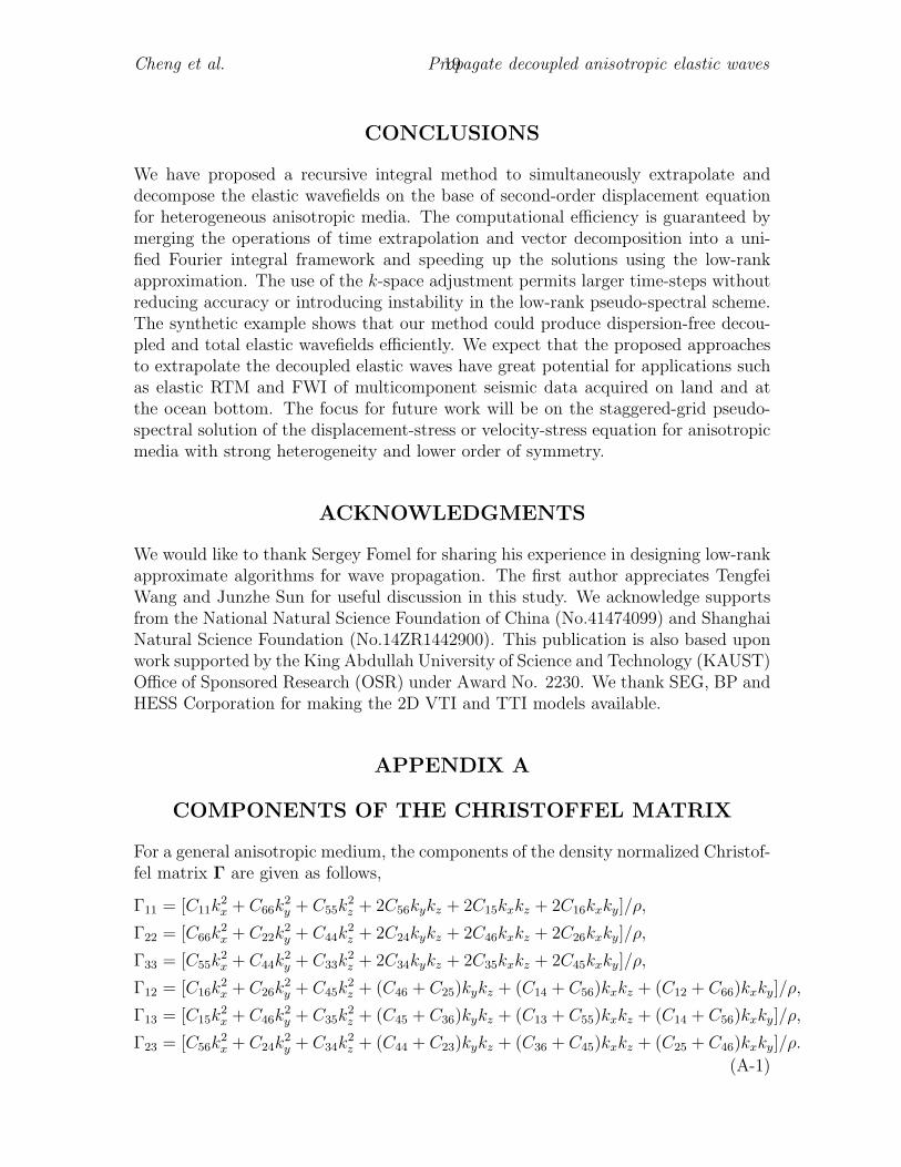
For a general anisotropic medium, the components of the density normalized Christof-fel matrix Γ are given as follows,

Γ11 = [C11k2x + C66k

2y + C55k

2z + 2C56kykz + 2C15kxkz + 2C16kxky]/ρ,

Γ22 = [C66k2x + C22k

2y + C44k


Γ33 = [C55k2x + C44k

2y + C33k


Γ12 = [C16k2x + C26k

2y + C45k

2z + (C46 + C25)kykz + (C14 + C56)kxkz + (C12 + C66)kxky]/ρ,

Γ13 = [C15k2x + C46k

2y + C35k

2z + (C45 + C36)kykz + (C13 + C55)kxkz + (C14 + C56)kxky]/ρ,

Γ23 = [C56k2x + C24k

2y + C34k

2z + (C44 + C23)kykz + (C36 + C45)kxkz + (C25 + C46)kxky]/ρ.

(A-1)


APPENDIX B

EXTENDED FORMULATIONS OF THEPSEUDO-SPECTRAL OPERATORS

According to equations 6 and 8, we express the pseudo-spectral operator that can beused to extrapolate the coupled elastic wavefields in its extended formation:

ux(x, t+ ∆t) = −ux(x, t−∆t) +∫eikxwxx(x,k)ux(k, t) dk

+∫eikxwxy(x,k)uy(k, t) dk +

∫eikxwxz(x,k)uz(k, t) dk,

uy(x, t+ ∆t) = −uy(x, t−∆t) +∫eikxwxy(x,k)ux(k, t) dk

+∫eikxwyy(x,k)uy(k, t) dk +

∫eikxwyz(x,k)uz(k, t) dk,

uz(x, t+ ∆t) = −uz(x, t−∆t) +∫eikxwxz(x,k)ux(k, t) dk

+∫eikxwyz(x,k)uy(k, t) dk +

∫eikxwzz(x,k)uz(k, t) dk,

(B-1)

in which ux(k, t), uy(k, t) and uz(k, t) represent the three components of the elasticwavefields in wavenumber-domain at the time of t.

For a VTI or orthorhombic medium, we express the stiffness tensor as a Voigtmatrix:

C =

C11 C12 C13 0 0 0C12 C22 C23 0 0 0C13 C23 C33 0 0 00 0 0 C44 0 00 0 0 0 C55 00 0 0 0 0 C66

, (B-2)

in which there are only five independent coefficient with C12 = C11−2C66, C22 = C11,C23 = C13 and C55 = C44, for a VTI medium. Therefore, the propagation matrix hasthe following extended formulation,

wxx(k) = 2−∆t2[C11k2x + C66k

2y + C55k

2z ],

wyy(k) = 2−∆t2[C66k2x + C22k

2y + C44k

2z ],

wzz(k) = 2−∆t2[C55k2x + C44k

2y + C33k

2z ],

wxy(k) = −∆t2[C12 + C66]kxky,wxz(k) = −∆t2[C13 + C55]kxkz,wyz(k) = −∆t2[C23 + C44]kykz.

(B-3)

If the principal axes of the medium are not aligned with the Cartesian axes, e.g.,for the tilted TI and orthorhombic media, we should apply the Bond transformation(Winterstein, 1990; Carcione, 2007) to get the stiffness matrix under the Cartesiansystem. This will introduce more mixed partial derivative terms in the wave equation,which demands lots of computational effort if a finite-difference algorithm is usedto extrapolate the wavefields. Fortunately, for the pseudo-spectral solution, it onlyintroduces negligible computation to prepare the propagation matrix and no extracomputation for the wavefield extrapolation.


Similarly, we can write the propagation matrix w(m)ij (in equation 20) for the

decoupled elastic waves in its extended formulation:

w(m)xx (x,k) = d

(m)xx (x,k)wxx(x,k) + d

(m)xy (x,k)wxy(x,k) + d

(m)xz (x,k)wxz(x,k),

w(m)xy (x,k) = d

(m)xx (x,k)wxy(x,k) + d

(m)xy (x,k)wyy(x,k) + d

(m)xz (x,k)wyz(x,k),

w(m)xz (x,k) = d

(m)xx (x,k)wxz(x,k) + d

(m)xy (x,k)wyz(x,k) + d

(m)xz (x,k)wzz(x,k),

w(m)yx (x,k) = d

(m)xy (x,k)wxx(x,k) + d

(m)yy (x,k)wxy(x,k) + d

(m)yz (x,k)wxz(x,k),

w(m)yy (x,k) = d

(m)xy (x,k)wxy(x,k) + d

(m)yy (x,k)wyy(x,k) + d

(m)yz (x,k)wyz(x,k),

w(m)yz (x,k) = d

(m)xy (x,k)wxz(x,k) + d

(m)yy (x,k)wyz(x,k) + d

(m)yz (x,k)wzz(x,k),

w(m)zx (x,k) = d

(m)xz (x,k)wxx(x,k) + d

(m)yz (x,k)wxy(x,k) + d

(m)zz (x,k)wxz(x,k),

w(m)zy (x,k) = d

(m)xz (x,k)wxy(x,k) + d

(m)yz (x,k)wyy(x,k) + d

(m)zz (x,k)wyz(x,k),

w(m)zz (x,k) = d

(m)xz (x,k)wxz(x,k) + d

(m)yz (x,k)wyz(x,k) + d

(m)zz (x,k)wzz(x,k).

(B-4)

APPENDIX C

K-SPACE ADJUSTMENT TO THE PSEUDO-SPECTRALSOLUTION

According to the eigen-decomposition of the Christoffel matrix (see Equations 9 to12), we can obtain the scalar wavefields for homogeneous anisotropic media using thetheory of mode separation (Dellinger and Etgen, 1990),

ui = Qijuj, (C-1)

in which ui with i = 1, 2, 3 represents the scalar qP-, qS1- and qS2-wave fields. Sothese wavefields satisfy the same scalar wave equation

∂2ttui + (vik)2ui = 0. (C-2)

The standard leapfrog scheme for this equation can be expressed as

u(n+1)

i − 2u(n)

i + u(n−1)

i

∆t2= −λ2

i u(n)

i . (C-3)

It is well known that this solution is limited to small time-steps for stable wavepropagation.

Fortunately, there is an exact time-steping solution for the second-order timederivatives allowing for any size of time-steps for homogeneous medium (Cox et al.,2007; Etgen and Brandsberg-Dahl, 2009), namely:

u(n+1)

i − 2u(n)

i + u(n−1)

i

∆t2=− sin2(λi∆t/2)

(∆t/2)2u

(n)

i . (C-4)


Comparing equations C-3 and C-4 shows that, it is possible to extend the length oftime-step without reducing the accuracy by replacing (λi∆t/2)2 with sin2 (λi∆t/2).This opens up a possibility by replacing k2 with k2sinc2(λi∆t/2) as a k-space adjust-ment to the spatial derivatives, which may convert the time-stepping pseudo-spectralsolution into an exact one for homogeneous media, and stable for larger time-steps(for a given level of accuracy) in heterogeneous media (Bojarski, 1982).

Nowadays, the k-space scheme is widely used to improve the approximation of thetemporal derivative in acoustic and ultrasound (Tabei et al., 2002; Cox et al., 2007;Fang et al., 2014). As far as we know, Liu (1995) was the first to apply k-space ideasto elastic wave problems. He derived a k-space form of the dyadic Green’s function forthe second-order wave equation and used it to calculate the scattered field iterativelyin a Born series. Firouzi et al. (2012) proposed a k-space scheme on the base of thefirst-order elastic wave equation for isotropic media.

Accordingly, we apply the k-space adjustment to improve the performance ofour two-step time-marching pseudo-spectral solution of the anisotropic elastic waveequation. To propagate the elastic waves on the base of equations 6 and 8, we needmodify the eigenvalues of Christoffel matrix as in Equation 14.


REFERENCES

Aki, K., and P. Richards, 1980, Quantitative Seismology (second edition): UniversityScience Books.

Bale, R. A., 2003, Modeling 3D anisotropic elastic data using the pseudospectralapproach: 70th EAGE Conference and Exhibition 2008, Expanded Abstracts.

Bojarski, N. N., 1982, The k-space formulation of the scattering problem in the timedomain: Journal of Acoustic Society of America, 72, 570–584.

Carcione, J. M., 1999, Staggered mesh for the anisotropic and viscoelastic wave equa-tion: Geophysics, 64, 1863–1866.

——–, 2007, Wave fields in real media: Wave propagation in anisotropic, anelastic,porous and electromagnetic media: Elsevier Ltd.

Cheng, J. B., and S. Fomel, 2014, Fast algorithms of elastic wave mode separation andvector decomposition using low-rank approximation for anisotropic media: Geo-physics, 79, C97–C110.

Cheng, J. B., and W. Kang, 2014, Simulating propagation of separated wave modesin general anisotropic media, Part I: P-wave propagators: Geophysics, 79, C1–C18.

Chu, C., B. Macy, and P. Anno, 2011, An accurate and stable wave equation forpure acoustic TTI modleing: 81st Annual International Meeting, SEG, ExpandedAbstracts, 179–184.

Cox, B. T., S. Kara, S. R. Arridge, and P. C. Beard, 2007, K-space propagation modelsfor acoustically heterogeneous media: Application to biomedical photoacoustics:Journal of Accoustic Society of America, 121, 3453–3464.

Crampin, S., 1991, Effects of point singularities on shear-wave propagation in sedi-mentary basin: Geophys. J. Int., 107, 531–543.

Dablain, M. A., 1986, The application of high-order differencing to the scalar waveequation: Geophysics, 51, 54–66.

Dellinger, J., and J. Etgen, 1990, Wavefield separation in two-dimensional anisotropicmedia: Geophysics, 55, 914–919.

Du, X., P. J. Fowler, and R. P. Fletcher, 2014, Recursive integral time-extrapolationmethods for waves: A comparative review: Geophysics, 79, T9–T26.

Engquist, B., and L. Ying, 2009, A fast directional algorithm for high frequencyacoustic scattering in two dimensionsr: Communications Mathematical Sciences,7, 327–345.

Etgen, J., and S. Brandsberg-Dahl, 2009, The pseudo-analytical method: Applicationof pseudo-Laplacians to acoustic and acoustic anisotropic wave propagation: 79thAnnual International Meeting, SEG, Expanded Abstracts, 2552–2556.

Fang, G., S. Fomel, Q. Z. Du, and J. W. Hu, 2014, Lowrank seismic wave extrapolationon a staggered grid: Geophysics, 79, T157–T168.

Firouzi, K., B. T. Cox, B. E. Treeby, and N. Saffari, 2012, A first-order k-space modelfor elastic wave propagation in heterogeneous media: Journal of Acoustic Societyof America, 132, 1271–1283.

Fomel, S., L. Ying, and X. Song, 2013, Seismic wave extrapolation using lowranksymbol approximation: Geophysical Prospecting, 1–11.

Fowler, P., and R. King, 2011, Modeling and reverse time migration of orthorhom-


bic pseudo-acoustic P-waves: 81st Annual International Meeting, SEG, ExpandedAbstracts, 190–195.

Kang, W., and J. B. Cheng, 2012, Propagating pure wave modes in 3D generalanisotropic media, Part II: SV and SH wave: 82nd Annual International Meeting,SEG, Expanded Abstracts, 1234–1238.

Kosloff, D., A. Q. Filho, E. Tessmer, and A. Behle, 1989, Numerical solution of theacoustic and elastic wave equation a new rapid expansion method: GeophysicalProspecting, 37, 383–394.

Liu, F., S. Morton, S. Jiang, L. Ni, and J. Leveille, 2009, Decoupled wave equationsfor P and SV waves in an acoustic VTI media: 79th Annual International Meeting,SEG, Expanded Abstracts, 2844–2848.

Liu, Q., 1995, Generalization of the k-space formulation to elastodynamic scatteringproblems: Journal of Acoustic Society of America, 97, 1373–1379.

Liu, Y., and C. Li, 2000, Study of elastic wave propagation in two-phase anisotropicmedia by numerical modeling of pseudospectral method: Acta Seismologica Sinica,13, 143–150.

Ma, D. T., and G. M. Zhu, 2003, P- and s-wave separated elastic wave equationnumerical modeling (in Chinese): Oil Geophysical Prospecting, 38, 482–486.

Ozdenvar, T., and G. McMechan, 1996, Causes and reduction of numerical artifacts inpseudo-spectral wavefield extrapolation: Geophysical Journal International, 126,819–829.

Schoenberg, M., and K. Helbig, 1997, Orthorhombic media: Modeling elastic wavebehavior in a vertically fractured earth: Geophysics, 62, 1954–1974.

Song, X., and T. Alkhalifah, 2013, Modeling of pseudoacoustic p-waves in orthorhom-bic media with a low-rank approximation: Geophysics, 78, C33–C40.

Sun, J., and S. Fomel, 2013, Low-rank one-step wave extrapolation: 83rd AnnualInternational Meeting, SEG, Expanded Abstracts, 1123–1127.

Sun, R., and G. A. McMechan, 2001, Scalar reverse-time depth migration of prestackelastic seismic data: Geophysics, 66, 1514–1527.

Tabei, M., T. D. Mast, and R. C. Waag, 2002, A k-space method for coupled first-roder acoustic propagation equations: Journal of Acoustic Society of America, 111,56–63.

Tsvankin, I., 2001, Seismic signatures and analysis of reflection data in anisotropiocmedia: Elsevier Science Ltd.

Wang, T. F., and J. B. Cheng, 2015, Elastic wave mode decoupling for full waveforminversion: 85th SEG Annual International Meeting, Expanded Abstracts, 1461–1466.

Wapenaar, C. P. A., N. A. Kinneging, and A. J. Berkhout, 1987, Principle of prestackmigration based on the full elastic two-way wave equation: Geophysics, 52, 151–173.

Winterstein, D., 1990, Velocity anisotropy terminology for geophysicists: Geophysics,55, 1070–1088.

Wu, Z., and T. Alkhalifah, 2014, The optimized expansion based low rank methodfor wavefield extrapolation: Geophysics, 79, T51–T60.

Xu, S., and H. Zhou, 2014, Accurate simulations of pure quasi-p-waves in complex


anisotropic media: Geophysics, 79, T341–T348.Yan, J., and P. Sava, 2008, Isotropic angle domain elastic reverse time migration:

Geophysics, 73, S229–S239.——–, 2009, Elastic wave-mode separation for VTI media: Geophysics, 74, WB19–

WB32.——–, 2011, Improving the efficiency of elastic wave-mode separation for heterogenous

tilted transverse isotropic media: Geophysics, 76, T65–T78.Zhan, G., R. C. Pestana, and P. L. Stoffa, 2012, Decoupled equations for reverse time

migration in tilted transversely isotropic media: Geophysics, 77, T37–T45.Zhang, J., Z. Tian, and C. Wang, 2007, P- and s-wave separated elastic wave equation

numerical modeling using 2d staggered-grid: 77th Annual International Meeting,SEG, Expanded Abstracts, 2104–2108.

Zhang, Q., and G. A. McMechan, 2010, 2D and 3D elastic wavefield vector decom-position in the wavenumber domain for VTI media: Geophysics, 75, D13–D26.

Zhang, Y., and G. Zhang, 2009, One-step extrapolation method for reverse timemigration: Geophysics, 74, A29–A33.

simulating propagation of decoupled elastic waves … propagation of decoupled elastic waves using...

Documents