INSTITUTE OF PHYSICS PUBLISHING PHYSICS IN MEDICINE AND BIOLOGY

Phys. Med. Biol. 51 (2006) 2237–2252 doi:10.1088/0031-9155/51/9/009

Simulation and visualization of dose uncertainties dueto interfractional organ motion

D Maleike, J Unkelbach and U Oelfke

Department of Medical Physics in Radiation Oncology, German Cancer Research Center(DKFZ), Im Neuenheimer Feld 280, 69120 Heidelberg, Germany

E-mail: d.maleike@dkfz.de, j.unkelbach@dkfz.de and u.oelfke@dkfz.de

Received 19 September 2005, in final form 16 March 2006Published 19 April 2006Online at stacks.iop.org/PMB/51/2237

AbstractIn this paper, we deal with the effects of interfractional organ motion duringradiation therapy. We consider two problems: first, treatment plan evaluationin the presence of motion, and second, the incorporation of organ motioninto IMRT optimization. Concerning treatment plan evaluation, we face theproblem that the delivered dose cannot be predicted with certainty at the time oftreatment planning but is associated with uncertainties. We present a methodto simulate stochastic properties of the dose distribution. This provides thetreatment planner with information about motion-related risks of different plansand may support the decision for or against a treatment plan. This informationincludes the display of probabilities of individual voxels to receive doses froma therapeutical interval or above critical levels, as well as a diagram that showsthe variability of the dose volume histogram. Concerning the incorporation oforgan motion into IMRT planning, we further analyse the approach of inverseplanning based on probability distributions of possible patient geometries.We consider three different sources of uncertainty, namely uncertainty aboutthe amplitude of motion, a systematic error and a random error. We analysethe impact of these sources of uncertainty on the optimized treatment plans forprostate cancer.

1. Introduction

In fractionated radiation therapy, treatment results are affected by organ motion, which occursduring treatment. Although this is a well-known fact, treatment plans are regularly evaluatedin terms of a single dose distribution, which shows the dose that would be delivered if thepatient’s geometry was always like in the planning CT scan. As the patient’s geometry mayvary between the fractions of a treatment (or during dose delivery in a single fraction), and

0031-9155/06/092237+16$30.00 © 2006 IOP Publishing Ltd Printed in the UK 2237

2238 D Maleike et al

because these variations cannot be known prior to treatment, there are usually differencesbetween the planned and the finally realized dose distribution (Langen and Jones 2001).

In this paper, we propose a method to overcome this simplified notion. In the presence oforgan motion, the delivered dose distribution is uncertain. The dose delivered to an elementof tissue must be considered as a random variable. We present tools to assess the stochasticcharacteristics of a dose distribution.

A mathematical model to describe organ motion induced geometric changes of the patientis the basis of an improved description of organ motion effects on the dose distribution. Withmodern imaging modalities inside the treatment room, it is possible to acquire several imagedata sets of a patient prior to or during the first fractions of a treatment, with the patient inthe treatment position. We assume that we have a set of such images, which can be used toestimate the parameters of the model of interfractional organ motion. In order to characterizethe potentially delivered dose distribution, we simulate a large number of treatments withrandom motion parameters, drawn from the motion model.

Another aspect of this paper is the inclusion of organ motion into the treatment planningprocess. In this context, the current paper is the fourth paper in a series of papers dealingwith the inclusion of organ motion in IMRT optimization (the previous papers are Unkelbachand Oelfke (2004, 2005a, 2005b)). The current paper is thus an extension of the previouslypublished work. In order to minimize redundancy, this paper is not self-contained but refersto a large extent to the previously published work. In the previous papers, we consideredthree types of errors that occur due to interfractional organ motion: first, random errorsthat describe random displacements of the tumour in different fractions; second, systematicerrors that describe a shift of the true mean position of the tumour from its estimatedmean position; and third, uncertainties in the magnitude of interfractional organ motion.In Unkelbach and Oelfke (2005a), we applied the concept of Bayesian inference to formulatea motion model that describes all three types of errors within a unified framework. Themotion model was used to calculate the expectation value of the dose distribution and itsvariance as a measure of the uncertainty of the dose prediction. The incorporation ofinterfractional motion into IMRT optimization was demonstrated for a model of idealizedgeometry. In Unkelbach and Oelfke (2005b), we considered the application of the conceptto clinical data of prostate patients. However, in this first application, we discussed randomerrors in detail, but we neglected systematic errors and uncertainties in the magnitude ofmotion.

In the current paper, we deal with the inclusion of systematic errors and an uncertainmagnitude of motion into treatment plan optimization and evaluation for prostate cancer. Thepaper contains two major result parts. In section 3.2, we focus on the incorporation of organmotion into IMRT optimization. We analyse the impact of the three types of uncertaintieson the optimized treatment plan. In brief, this part represents the transfer of the conceptdeveloped in Unkelbach and Oelfke (2005a) from an idealized geometric model to clinicaldata of prostate patients. In section 3.1, we investigate problems in treatment plan evaluationthat generally occur in the presence of interfractional motion, independent of the foregoingtreatment plan optimization method. The dose distribution becomes a random variable, whichrepresents the underlying problem in treatment plan evaluation. In a first step, the dosedelivered to a voxel can be characterized by an expectation value of the dose and its variance.However, this information may not always be easy to interpret. Therefore, we provideadditional surrogates to characterize the dose. For example, we display the probabilitythat the dose delivered to a voxel is within predefined dose intervals. Such illustrationsallow for an estimation of sufficient target coverage and the risk of overdosing criticalstructures.

Simulation and visualization of dose uncertainties 2239

2. Materials and methods

In this section, we describe methods to calculate stochastic properties of a dose distributionfor a given treatment plan. Section 2.1 summarizes the assumptions on the treatment planningprocess, section 2.2 introduces the mathematical model of internal organ motion, which isdescribed in detail in Unkelbach and Oelfke (2005a). Sections 2.3–2.5 describe the methodsused to calculate characteristics of the random variable dose distribution based on the motionmodel. Section 2.6 concerns the inverse IMRT planning concept in order to include the motionmodel in the treatment plan optimization.

2.1. Assumptions on the treatment process

Concerning the treatment process, we apply the assumptions introduced in a previous paper(Unkelbach and Oelfke 2004) dealing with IMRT optimization for prostate cancer. The mostimportant aspects are repeated here for convenience.

• There are one or more planning CT scans at the time of treatment planning, i.e. oneplanning CT scan plus additional verification scans.

• For more than one CT, voxel positions in the first CT are matched with their correspondingvoxels in the other images. The resulting set of vectors can be used to estimate parametersof a motion model.

• A treatment plan defines a constant dose distribution in space, which we refer to as thestatic dose distribution, denoted by Dstat. The static dose distribution is calculated on theplanning CT scan and is assumed to be unaffected by changes of the patient geometry indifferent fractions. Tissue elements move through this ‘dose cloud’ and accumulate dose.For prostate patients, this approximation may be justified. For a discussion of the validityof the ‘dose cloud’ method, see e.g. Bortfeld et al (2004) and the notes in the previouspaper (Unkelbach and Oelfke 2005b, section IIA).

• Intrafractional organ motion is neglected.

2.2. The model of organ motion

We apply the motion model introduced in Unkelbach and Oelfke (2005a); this section onlyrecalls the results and the notation needed for following sections. Movement of tissue isdescribed as a movement of individual volume elements. Each volume element can be locatedat different positions r and the movement is assumed to be Gaussian, i.e. there is an assumedmean position of the tissue element r = (x, y, z) plus a random displacement r − r, which isnormally distributed around zero.

In this paper, we consider the simplified case that random displacements are uncorrelatedin the three spatial dimensions, so that the probability distribution for a three-dimensionaldisplacement factorizes. Therefore, we provide the formulae for a single coordinate x only.For a generalization to correlated movements in three dimensions, see Lam et al (2005). Theprobability of finding a certain tissue element at a position x can be described as

P(x|x, σx) = 1√2πσx

exp

(− (x − x)2

2σ 2x

). (1)

The parameters of this model (x and σx) have to be estimated from the patient images thatare obtained prior to the simulation of a plan’s uncertainties. After registration of the patientimages, there should be a set of M measured positions {pxµ}Mµ=1 for the tissue element.

For the practical estimation of x and σx , we use the technique of Bayesian inference,which takes into account the inevitable estimation errors. The method yields not single

2240 D Maleike et al

estimated values, but probability distributions P(x|σx, {pxµ}) and P(σx |{pxµ}), describinghow probable each pair of parameters is—given the data measured from the patient imagesand (optionally) data about organ motion in previous patients.

The probability that x is the ‘true’ mean position of the tissue element is given by

P(x|x, σx) = 1√2π

σ 2x

M

exp

(− (x − x)2

2 σ 2x

M

), (2)

where x = 1M

∑Mµ=1 pxµ is the mean position of the voxel as estimated by the arithmetic mean

of the measured voxel positions in the individual images. P(x|x, σx) describes systematicerrors.

We consider two situations for the calculation of the probability distribution P(σx |{pxµ})for the amplitude of motion: estimation based on the patient images alone and estimationbased on patient images plus motion data from previous patients.

When we base the estimation on the measured positions pxµ alone, we get

P(σx

∣∣σ datax

) ∝ 1

(√

2πσx)M−1exp

(−

(σ data

x

)2

2 1M

σ 2x

), (3)

where(σ data

x

)2 = 1M

∑Mµ=1(pxµ − x)2 is the magnitude of motion estimated from the patient

images.However, there are many motion studies, performed for a variety of organs (Tinger et al

1998, Roeske et al 1995). Thus, it is sensible to incorporate prior knowledge about σ (whichis often reported in studies) into the model. This means considering some a priori distributionP(σx), which describes the probabilities of different values of σx independent of the individualpatient. Using a gamma prior, the estimation for σx is

P(σx

∣∣σ datax

) ∝ σα−1x

(√

2πσx)M−1exp(−λσx) exp

(−

(σ data

x

)2

2 1M

σ 2x

). (4)

Both parameters α and λ of the gamma prior can be expressed in terms of the expectationvalue σ

popx and the standard deviation σ var

x of the prior distribution P(σx) for a population ofpatients:

α =(σ

popx

)2(σ var

x

)2 and λ = σpopx(

σ varx

)2 . (5)

For uncorrelated movement in the three spatial directions, the probability to find a tissueelement at the three-dimensional position r = (x, y, z) given a mean position r = (x, y, z) isgiven by

P(r|r, σ) = P(x|x, σx)P (y|y, σy)P (z|z, σz). (6)

Also, the probability distributions P(r|σ, r) and P(σ|σdata) factorize:

P(r|r, σ) = P(x|x, σx)P (y|y, σy)P (z|z, σz), (7)

P(σ|σdata) = P(σx

∣∣σ datax

)P

(σy

∣∣σ datay

)P

(σz

∣∣σ dataz

). (8)

For the general case, P(r|r, σ) and P(r|σ, r) are given by three-dimensional multivariatenormal distributions and P(σ|σdata) is given by a Wishard distribution.

In the case that a structure can only move as a rigid body, all tissue elements in thisstructure are characterized by the same parameter value for σdata. Tissue deformations canbe described by allowing for different motion amplitudes σdata for different elements of astructure.

Simulation and visualization of dose uncertainties 2241

2.3. The expectation value and the variance of the dose

Based on the motion model and a given static dose distribution, we can formally define theexpectation value of the cumulative dose after N fractions in a certain tissue element:

〈D〉 =∫

· · ·∫

1

N

N∑µ=1

Dstat(rµ)

N∏

µ=1

P(rµ|r, σ)P (r|σ, r)P (σ|σdata)

N∏µ=1

drµ dr dσ.

(9)

The dose Dstat(r) refers to the dose value of the static dose field at position r. The varianceof the cumulative dose is given by

V = (〈D2〉 − 〈D〉2), (10)

where

〈D2〉 =∫

· · ·∫

1

N

N∑µ=1

Dstat(rµ)

2N∏

µ=1

P(rµ|r, σ)P (r|σ, r)P (σ|σdata)

N∏µ=1

drµ dr dσ.

(11)

The standard deviation of the dose is the square root of the variance (SD = √V ).

2.4. Simulation of stochastic properties

Due to the stochastic nature of interfractional organ motion, the dose applied to a tissue elementis a random variable. We have to find appropriate surrogates to characterize the random variable‘dose to a tissue element’. Here, we want to calculate three types of characteristics.

(i) The expected value of the dose received by individual tissue elements.(ii) The corresponding standard deviation of the dose received by individual tissue elements.

(iii) The probability for individual tissue elements of receiving doses within defined doseintervals.

In order to calculate these quantities based on the motion model and a given static dosedistribution, we implemented a stand-alone program. Concerning the expectation value andthe variance of the dose, the tool performs an evaluation of the integrals in equations (9) and(11) by Monte Carlo simulation. The algorithm works as follows: repeat steps (i)–(iv) Qtimes1.

(i) Randomly generate a ‘true’ amplitude of motion σ = (σx, σy, σz). If prior knowledgeabout the amplitude of motion is available, use equation (4), otherwise use equation (3)(for M = 1 CTs one must have prior knowledge, since one cannot estimate the magnitudeof motion from one data point).

(ii) Use σ from step (i) to randomly generate a ‘true’ mean position r. Use equation (2).(iii) Use the complete motion model from steps (i) and (ii) to generate N random treatment

positions rµ from equation (1).(iv) Accumulate the total dose for these treatment positions from the static dose distribution

(q is an index for the simulation number):

Dq = 1

N

N∑µ=1

Dstat(rµ). (12)

The static dose distribution is assumed to be constant within a static voxel, i.e. nointerpolation between neighbouring voxels is implemented.

1 We choose Q in the order of 10 000.

2242 D Maleike et al

Basically, this simulation is done for every single tissue element2. For example, for theexpectation values of the dose in different tissue elements, we have to display a 3D spatialdistribution of expectation values. The result has to be interpreted within a moving, tissue-fixed coordinate system. Each tissue element has its fixed position within this system, andwhen tissue elements move, they change positions only in the static coordinate system ofthe treatment room where the static dose distribution is defined. Practically, we associateeach voxel in the planning CT with a tissue element and then apply the planning CT scan tovisualize the spatial distribution of dose expectation values in the deforming tissue.

For the generation of random numbers, we use two different techniques. For thedistributions in equations (3) and (4), we utilize the rejection method, which is a generalpurpose method of random number generation, described in Press et al (1994, chapter 7.3).The numbers from a uniform distribution, which are needed for this method, are generatedby an implementation of the Mersenne twister algorithm (Matsumoto and Nishimura 1998),which was recommended in a recent review of random number generators (L’Ecuyer 2004,chapter 2). For the normal distribution, there are much faster algorithms available for randomnumber generation. We decided to use the FastNorm algorithm (Wallace 1996) because of itsspeed.

2.5. Simulation output

In this section, we describe the output of our simulations. Examples for these results will bepresented in section 3.1.

2.5.1. Expected value and standard deviation. The easiest way to characterize a stochasticquantity or a random variable is the expected value of that quantity, in our case the dose to avoxel. When predicting the outcome of a probability experiment, the expected value representsthe best possible guess, and this is the reason why we estimate it with our simulations.

Inherently connected with the expected value is the standard deviation, which describeshow far from the expected value actual realizations typically are. We estimate this measuretogether with the expected value, because it provides us a hint about the quality of theprediction by the expected value. If the standard deviation is small, the realizations of ourrandom variable will most probably be found in a small region around the expected value. Anincreased standard deviation indicates the spreading of the observed realizations around theexpected value.

According to the simulation procedure described in section 2.4, we estimate the expectedvalue of dose 〈D〉 and the standard deviation SD of a tissue element with

〈D〉 ≈ 1

Q

Q∑q=1

Dq (13)

and

SD =√

〈D2〉 − 〈D〉2, (14)

with

〈D2〉 ≈ 1

Q

Q∑q=1

D2q . (15)

2 Practically, we group voxels that are characterized by the same motion parameters σdata, σpop, and σvar. We thenuse the same displacements for these tissue elements to accumulate dose.

Simulation and visualization of dose uncertainties 2243

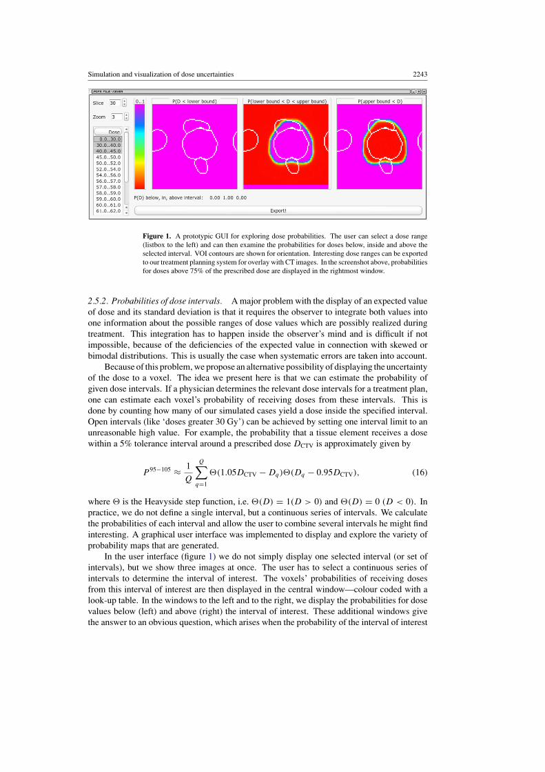
Figure 1. A prototypic GUI for exploring dose probabilities. The user can select a dose range(listbox to the left) and can then examine the probabilities for doses below, inside and above theselected interval. VOI contours are shown for orientation. Interesting dose ranges can be exportedto our treatment planning system for overlay with CT images. In the screenshot above, probabilitiesfor doses above 75% of the prescribed dose are displayed in the rightmost window.

2.5.2. Probabilities of dose intervals. A major problem with the display of an expected valueof dose and its standard deviation is that it requires the observer to integrate both values intoone information about the possible ranges of dose values which are possibly realized duringtreatment. This integration has to happen inside the observer’s mind and is difficult if notimpossible, because of the deficiencies of the expected value in connection with skewed orbimodal distributions. This is usually the case when systematic errors are taken into account.

Because of this problem, we propose an alternative possibility of displaying the uncertaintyof the dose to a voxel. The idea we present here is that we can estimate the probability ofgiven dose intervals. If a physician determines the relevant dose intervals for a treatment plan,one can estimate each voxel’s probability of receiving doses from these intervals. This isdone by counting how many of our simulated cases yield a dose inside the specified interval.Open intervals (like ‘doses greater 30 Gy’) can be achieved by setting one interval limit to anunreasonable high value. For example, the probability that a tissue element receives a dosewithin a 5% tolerance interval around a prescribed dose DCTV is approximately given by

P 95−105 ≈ 1

Q

Q∑q=1

�(1.05DCTV − Dq)�(Dq − 0.95DCTV), (16)

where � is the Heavyside step function, i.e. �(D) = 1(D > 0) and �(D) = 0 (D < 0). Inpractice, we do not define a single interval, but a continuous series of intervals. We calculatethe probabilities of each interval and allow the user to combine several intervals he might findinteresting. A graphical user interface was implemented to display and explore the variety ofprobability maps that are generated.

In the user interface (figure 1) we do not simply display one selected interval (or set ofintervals), but we show three images at once. The user has to select a continuous series ofintervals to determine the interval of interest. The voxels’ probabilities of receiving dosesfrom this interval of interest are then displayed in the central window—colour coded with alook-up table. In the windows to the left and to the right, we display the probabilities for dosevalues below (left) and above (right) the interval of interest. These additional windows givethe answer to an obvious question, which arises when the probability of the interval of interest

2244 D Maleike et al

is very low. In these cases, a user would probably want to know whether the dose will behigher or lower than the specified interval.

The advantage of these probability maps is that they can be displayed as a simple, intuitiveinformation. The user has not to integrate several pictures into one piece of information as withthe expected value and the standard deviations. Although we show three separate windows,each of them could be considered isolated, and each answers a single question, namely whatis the probability of receiving a dose within a given range.

2.6. Inclusion of organ motion into the optimization

In order to integrate organ motion into IMRT optimization, we further investigate the approachof inverse planning based on probability distributions of patient geometries which has beensubject to detailed investigation in the previous papers (Unkelbach and Oelfke 2004, 2005a,2005b). In comparison to Unkelbach and Oelfke (2005b), which deals with random errorsalone, we generalized the implementation in the inverse planning tool KonRad in order to dealwith systematic errors and uncertainties in the magnitude of motion.

For the optimization of the fluence maps, we adopt the quadratic objective function thatwas introduced in Unkelbach and Oelfke (2005b):

E =∑

i∈CTV

αCTV[(〈Di〉 − DCTV)2 + Vi] +∑

n

∑

i∈OARn

αn

(〈Di〉 − Dmaxn

)2+

, (17)

where(〈Di〉 − Dmax

n

)+ = (〈Di〉 − Dmax

n

)for 〈Di〉 > Dmax

n and(〈Di〉 − Dmax

n

)+ = 0 for

〈Di〉 < Dmaxn . DCTV is the dose prescribed to the tumour, Dmax

n is a maximum dose for theorgan at risk (OAR) with index n, and αCTV and αn are penalty factors for the CTV and organsat risk, respectively. Contoured organs at risk are rectum, bladder and the pelvic bones. Theunclassified tissue that surrounds the CTV and the contoured organs at risk is also treated asan organ at risk.

The index i refers to a tissue element, i.e. a voxel in the planning CT scan. The expectationvalue of the dose 〈Di〉 in voxel i is given by equation (9) and the variance Vi is given byequations (10) and (11). The objective function can be minimized by means of standardgradient methods. The expectation value 〈Di〉 can be expressed as a linear function of thebeamlet weights by defining an effective dose contribution matrix that stores the expectationvalue of the dose contribution of a beamlet to the voxel for unit fluence. The variance Vi isevaluated by defining a variance contribution tensor that stores the variance contribution ofa pair of beamlets to the voxel for unit fluence. The concept was described in Unkelbachand Oelfke (2005b) and the generalization to the extended motion model considered now isstraightforward. Exemplarily, the calculation of the variance contribution tensor is describedin the appendix.

3. Results

3.1. Tools for treatment plan evaluation

In this section, we demonstrate the application of the treatment plan evaluation tools describedin section 2. We consider a treatment plan that is optimized by minimizing the objectivefunction in equation (17). It is assumed that M = 5 CT scans are performed prior to treatmentand that the following set of motion model parameters was estimated from these images forall voxels: σdata = M−1

M(3 mm, 4 mm, 3 mm), where the x-coordinate corresponds to the LR

Simulation and visualization of dose uncertainties 2245

direction, the y-coordinate to the AP direction and the z-coordinate to the CC direction3. Noprior knowledge about the amplitude of motion is incorporated. The estimated mean positionsr for the tissue elements are assumed to be identical to their respective positions in the planningCT. The treatment plan is optimized for N = 30 fractions. For a clinical application, the 3Ddistribution for σdata and mean positions of the tissue elements had to be estimated from theimages of the individual patient as described in section 2.2. Due to ongoing work on elasticimage registration in our department, we have not yet realized this approach and demonstratethe treatment plan evaluation tools for this idealized movement.

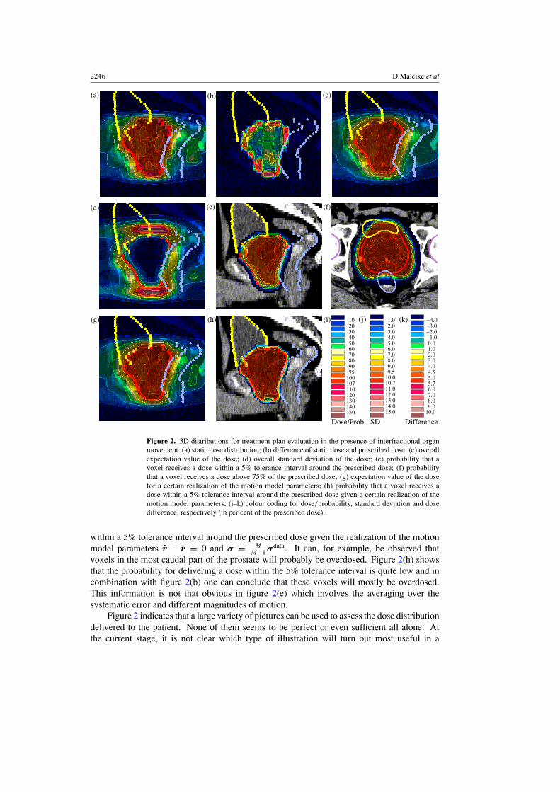
Figure 2(a) shows the static dose distribution of the optimized treatment plan for aprostate patient. As expected, the static dose distribution shows some moderate dose peaksat the edge of the tumour. The highest dose peaks are approximately 110% of the prescribeddose. In figure 2(b), the modulation pattern of the static dose field is illustrated in moredetail. It shows the difference of the static dose and the prescribed dose in each voxel. Thestatic dose distribution is important to understand the generic features of the probabilistictreatment planning approach. However, it is per definition not the dose distribution we expectto be realized in the patient. In the context of treatment plan evaluation we are primarilyinterested in assessing the dose that is finally delivered to the patient. We can look at theexpectation value of the dose (figure 2(c)) which provides the best estimate of the delivereddose for each voxel. The overall expectation value of the dose is relatively difficult to interpretbecause the expected dose can never be realized in all voxels simultaneously. The expectationvalue involves averaging over the systematic error and different magnitudes of motion. Thisaveraging process occurs only for a population of patients but not for the individual patient.The spatial 3D distribution of dose expectation values is therefore not a good surrogate forthe delivered dose distribution as a whole. It has to be interpreted for each voxel separately.Since we know that the expectation value is not realized, we can in addition look at the overalluncertainty of this dose prediction, too, i.e. the standard deviation in figure 2(d). The doseuncertainty is relatively small in the inner region of the CTV (in the order of 1–2% of theprescribed dose). At the edge of the CTV, the standard deviation is approximately 5% of theprescribed dose. The largest values occur in the adjacent healthy tissue above and belowthe CTV, with peaks of 10–15% of the prescribed dose.

One aspect of treatment plan evaluation is to ensure a sufficient target coverage. To assessthe target coverage, the treatment planner has to combine the information of the expectationvalue and the standard deviation. When the expected dose in a voxel is close to the prescribeddose and the standard deviation of the dose is small, this voxel will very likely receive asufficient dose. Figure 2(e) shows the probability that a voxel receives a dose within a5% tolerance interval around the prescribed dose. Such an illustration allows for directlyassessing the probability of sufficient target coverage. It may be a valuable tool for treatmentplan evaluation. Similar pictures can be used to estimate the risk for overdosing an organ atrisk. Figure 2(f) shows the probability that a voxel receives a dose above 75% of the prescribeddose.

Figure 2(g) shows the expectation value of the dose for a certain realization of the motionmodel parameters r and σ. We choose r − r = 0 and σ = M

M−1σdata. Thus, the blurring ofthe static dose distribution is due to the random error only. Figure 2(g) is therefore a bettersurrogate for the 3D dose distribution which may approximately be realized (in contrast tothe overall expectation value in figure 2(c)). However, it does not contain the informationabout the systematic error. Figure 2(h) shows the probability that a voxel receives a dose

3 The factor M−1M

is introduced in order to make 3 mm and 4 mm the unbiased estimates of the standard deviationof voxel displacements whereas σdata refers to the maximum likelihood estimate (Unkelbach and Oelfke 2005a).

2246 D Maleike et al

10.711.0

10.0

12.013.014.015.0

9.59.08.07.06.05.04.03.02.01.0

107110

100

120130140150

95908070605040302010

10.0

0.01.02.03.04.04.5

5.75.0

6.07.08.09.0

−1.0−2.0−3.0−4.0

(b) (c)(a)

(e) (f)(d)

(g) (h) (i) (k)(j)

Dose/Prob SD Difference

Figure 2. 3D distributions for treatment plan evaluation in the presence of interfractional organmovement: (a) static dose distribution; (b) difference of static dose and prescribed dose; (c) overallexpectation value of the dose; (d) overall standard deviation of the dose; (e) probability that avoxel receives a dose within a 5% tolerance interval around the prescribed dose; (f) probabilitythat a voxel receives a dose above 75% of the prescribed dose; (g) expectation value of the dosefor a certain realization of the motion model parameters; (h) probability that a voxel receives adose within a 5% tolerance interval around the prescribed dose given a certain realization of themotion model parameters; (i–k) colour coding for dose/probability, standard deviation and dosedifference, respectively (in per cent of the prescribed dose).

within a 5% tolerance interval around the prescribed dose given the realization of the motionmodel parameters r − r = 0 and σ = M

M−1σdata. It can, for example, be observed thatvoxels in the most caudal part of the prostate will probably be overdosed. Figure 2(h) showsthat the probability for delivering a dose within the 5% tolerance interval is quite low and incombination with figure 2(b) one can conclude that these voxels will mostly be overdosed.This information is not that obvious in figure 2(e) which involves the averaging over thesystematic error and different magnitudes of motion.

Figure 2 indicates that a large variety of pictures can be used to assess the dose distributiondelivered to the patient. None of them seems to be perfect or even sufficient all alone. Atthe current stage, it is not clear which type of illustration will turn out most useful in a

Simulation and visualization of dose uncertainties 2247

(c)(a) (b)

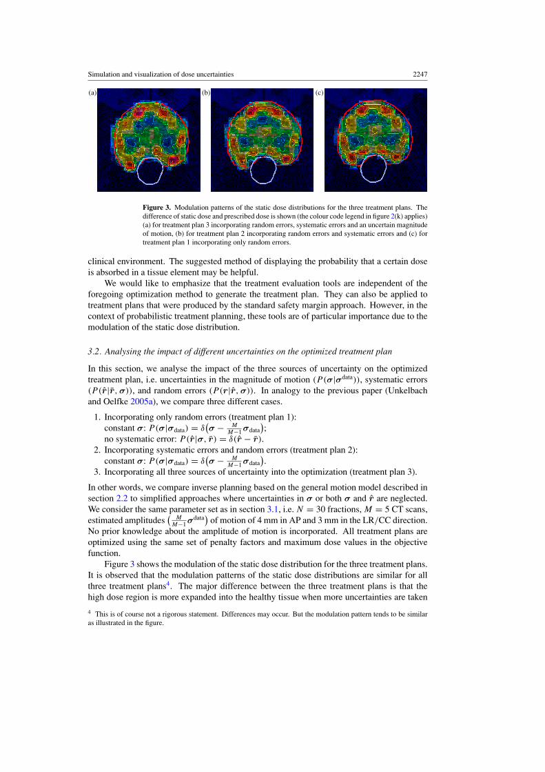
Figure 3. Modulation patterns of the static dose distributions for the three treatment plans. Thedifference of static dose and prescribed dose is shown (the colour code legend in figure 2(k) applies)(a) for treatment plan 3 incorporating random errors, systematic errors and an uncertain magnitudeof motion, (b) for treatment plan 2 incorporating random errors and systematic errors and (c) fortreatment plan 1 incorporating only random errors.

clinical environment. The suggested method of displaying the probability that a certain doseis absorbed in a tissue element may be helpful.

We would like to emphasize that the treatment evaluation tools are independent of theforegoing optimization method to generate the treatment plan. They can also be applied totreatment plans that were produced by the standard safety margin approach. However, in thecontext of probabilistic treatment planning, these tools are of particular importance due to themodulation of the static dose distribution.

3.2. Analysing the impact of different uncertainties on the optimized treatment plan

In this section, we analyse the impact of the three sources of uncertainty on the optimizedtreatment plan, i.e. uncertainties in the magnitude of motion (P (σ|σdata)), systematic errors(P (r|r, σ)), and random errors (P (r|r, σ)). In analogy to the previous paper (Unkelbachand Oelfke 2005a), we compare three different cases.

1. Incorporating only random errors (treatment plan 1):constant σ: P(σ|σdata) = δ

(σ − M

M−1σdata);

no systematic error: P(r|σ, r) = δ(r − r).2. Incorporating systematic errors and random errors (treatment plan 2):

constant σ: P(σ|σdata) = δ(σ − M

M−1σdata).

3. Incorporating all three sources of uncertainty into the optimization (treatment plan 3).

In other words, we compare inverse planning based on the general motion model described insection 2.2 to simplified approaches where uncertainties in σ or both σ and r are neglected.We consider the same parameter set as in section 3.1, i.e. N = 30 fractions, M = 5 CT scans,estimated amplitudes

(M

M−1σdata)

of motion of 4 mm in AP and 3 mm in the LR/CC direction.No prior knowledge about the amplitude of motion is incorporated. All treatment plans areoptimized using the same set of penalty factors and maximum dose values in the objectivefunction.

Figure 3 shows the modulation of the static dose distribution for the three treatment plans.It is observed that the modulation patterns of the static dose distributions are similar for allthree treatment plans4. The major difference between the three treatment plans is that thehigh dose region is more expanded into the healthy tissue when more uncertainties are taken

4 This is of course not a rigorous statement. Differences may occur. But the modulation pattern tends to be similaras illustrated in the figure.

2248 D Maleike et al

0

20

40

60

80

100

120

140

0 20 40 60 80 100

prob

abili

ty [%

]

distance [mm]

all uncertaintiessystematic and randomonly randomtumour

0

2

4

6

8

10

12

0 20 40 60 80 100

SD

[% o

f pre

scrib

ed d

ose]

distance [mm]

all uncertaintiessystematic and randomonly randomtumour

(b)(a)

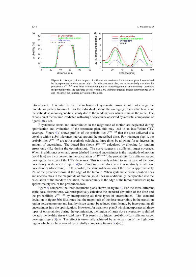
Figure 4. Analysis of the impact of different uncertainties for treatment plan 1 (optimizedby incorporating random errors only). For this treatment plan, we retrospectively calculate theprobability P 95−105 three times while allowing for an increasing amount of uncertainty: (a) showsthe probability that the delivered dose is within a 5% tolerance interval around the prescribed doseand (b) shows the standard deviation of the dose.

into account. It is intuitive that the inclusion of systematic errors should not change themodulation pattern too much. For the individual patient, the averaging process that levels outthe static dose inhomogeneities is only due to the random error which remains the same. Theexpansion of the volume irradiated with a high dose can be observed by a careful comparison offigures 3(a)–(c).

If systematic errors and uncertainties in the magnitude of motion are neglected duringoptimization and evaluation of the treatment plan, this may lead to an insufficient CTVcoverage. Figure 4(a) shows profiles of the probabilities P 95−105 that the dose delivered to avoxel is within a 5% tolerance interval around the prescribed dose. For treatment plan 1, theprobabilities P 95−105 are retrospectively calculated three times by allowing for an increasingamount of uncertainty. The dotted line shows P 95−105 calculated by allowing for randomerrors only (like during the optimization). The curve suggests a sufficient target coverage.When, in addition, systematic errors (dashed line) and uncertainties in the magnitude of motion(solid line) are incorporated in the calculation of P 95−105, the probability for sufficient targetcoverage at the edge of the CTV decreases. This is closely related to an increase of the doseuncertainty as depicted in figure 4(b). Random errors alone result in relatively small doseuncertainties (dotted line). In this profile, the standard deviation of the dose is approximately2% of the prescribed dose at the edge of the tumour. When systematic errors (dashed line)and uncertainties in the magnitude of motion (solid line) are additionally incorporated into thecalculation of the standard deviation, the uncertainty at the edge of the tumour increases up toapproximately 6% of the prescribed dose.

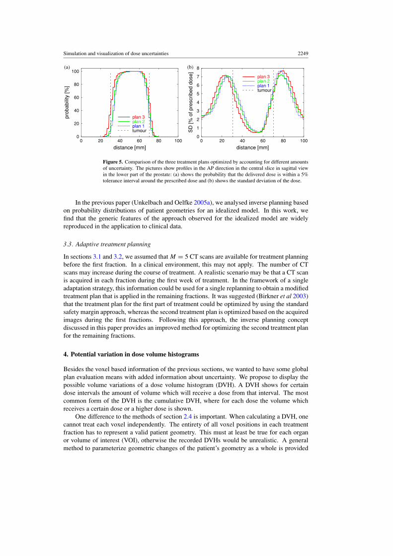
Figure 5 compares the three treatment plans shown in figure 3. For the three differentstatic dose distributions, we retrospectively calculate the standard deviation of the dose andthe probabilities P 95−105 by incorporating all three types of uncertainties. The standarddeviation in figure 5(b) illustrates that the magnitude of the dose uncertainty in the transitionregion between tumour and healthy tissue cannot be reduced significantly by incorporating alluncertainties into the optimization. However, for treatment plan 3 which incorporates all threetypes of uncertainties during the optimization, the region of large dose uncertainty is shiftedtowards the healthy tissue (solid line). This results in a higher probability for sufficient targetcoverage (figure 5(a)). The effect is essentially achieved by an expansion of the high doseregion which can be observed by carefully comparing figures 3(a)–(c).

Simulation and visualization of dose uncertainties 2249

0

20

40

60

80

100

0 20 40 60 80 100

prob

abili

ty [%

]

distance [mm]

plan 3plan 2plan 1tumour

0

1

2

3

4

5

6

7

8

0 20 40 60 80 100

SD

[% o

f pre

scrib

ed d

ose]

distance [mm]

plan 3plan 2plan 1tumour

(b)(a)

Figure 5. Comparison of the three treatment plans optimized by accounting for different amountsof uncertainty. The pictures show profiles in the AP direction in the central slice in sagittal viewin the lower part of the prostate: (a) shows the probability that the delivered dose is within a 5%tolerance interval around the prescribed dose and (b) shows the standard deviation of the dose.

In the previous paper (Unkelbach and Oelfke 2005a), we analysed inverse planning basedon probability distributions of patient geometries for an idealized model. In this work, wefind that the generic features of the approach observed for the idealized model are widelyreproduced in the application to clinical data.

3.3. Adaptive treatment planning

In sections 3.1 and 3.2, we assumed that M = 5 CT scans are available for treatment planningbefore the first fraction. In a clinical environment, this may not apply. The number of CTscans may increase during the course of treatment. A realistic scenario may be that a CT scanis acquired in each fraction during the first week of treatment. In the framework of a singleadaptation strategy, this information could be used for a single replanning to obtain a modifiedtreatment plan that is applied in the remaining fractions. It was suggested (Birkner et al 2003)that the treatment plan for the first part of treatment could be optimized by using the standardsafety margin approach, whereas the second treatment plan is optimized based on the acquiredimages during the first fractions. Following this approach, the inverse planning conceptdiscussed in this paper provides an improved method for optimizing the second treatment planfor the remaining fractions.

4. Potential variation in dose volume histograms

Besides the voxel based information of the previous sections, we wanted to have some globalplan evaluation means with added information about uncertainty. We propose to display thepossible volume variations of a dose volume histogram (DVH). A DVH shows for certaindose intervals the amount of volume which will receive a dose from that interval. The mostcommon form of the DVH is the cumulative DVH, where for each dose the volume whichreceives a certain dose or a higher dose is shown.

One difference to the methods of section 2.4 is important. When calculating a DVH, onecannot treat each voxel independently. The entirety of all voxel positions in each treatmentfraction has to represent a valid patient geometry. This must at least be true for each organor volume of interest (VOI), otherwise the recorded DVHs would be unrealistic. A generalmethod to parameterize geometric changes of the patient’s geometry as a whole is provided

2250 D Maleike et al

0

0.2

0.4

0.6

0.8

1

0.6 0.7 0.8 0.9 1 1.1

Vol

ume

[frac

tion]

Dose [fraction of prescribed dose]

Median75%-97.5% , 2.5%-25%

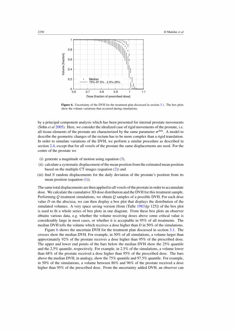
Figure 6. Uncertainty of the DVH for the treatment plan discussed in section 3.1. The box plotsshow the volume variations that occurred during simulations.

by a principal component analysis which has been presented for internal prostate movements(Sohn et al 2005). Here, we consider the idealized case of rigid movements of the prostate, i.e.all tissue elements of the prostate are characterized by the same parameter σdata. A model todescribe the geometric changes of the rectum has to be more complex than a rigid translation.In order to simulate variations of the DVH, we perform a similar procedure as described insection 2.4, except that for all voxels of the prostate the same displacements are used. For thecentre of the prostate we

(i) generate a magnitude of motion using equation (3),

(ii) calculate a systematic displacement of the mean position from the estimated mean positionbased on the multiple CT images (equation (2)) and

(iii) find N random displacements for the daily deviation of the prostate’s position from itsmean position (equation (1)).

The same total displacements are then applied to all voxels of the prostate in order to accumulatedose. We calculate the cumulative 3D dose distribution and the DVH for this treatment sample.Performing Q treatment simulations, we obtain Q samples of a possible DVH. For each dosevalue D on the abscissa, we can then display a box plot that displays the distribution of thesimulated volumes. A very space saving version (from (Tufte 1983)[p 125]) of the box plotis used to fit a whole series of box plots in one diagram. From these box plots an observerobtains various data, e.g. whether the volume receiving doses above some critical value isconsiderably large in most cases, or whether it is acceptable in 95% of all treatments. Themedian DVH tells the volume which receives a dose higher than D in 50% of the simulations.

Figure 6 shows the uncertain DVH for the treatment plan discussed in section 3.1. Thecrosses show the median DVH. For example, in 50% of all simulations, a volume larger thanapproximately 92% of the prostate receives a dose higher than 95% of the prescribed dose.The upper and lower end points of the bars below the median DVH show the 25% quantileand the 2.5% quantile, respectively. For example, in 2.5% of the simulations, a volume lowerthan 68% of the prostate received a dose higher than 95% of the prescribed dose. The barsabove the median DVH, in analogy, show the 75% quantile and 97.5% quantile. For example,in 50% of the simulations, a volume between 86% and 96% of the prostate received a dosehigher than 95% of the prescribed dose. From the uncertainty added DVH, an observer can

Simulation and visualization of dose uncertainties 2251

e.g. see whether a significant fraction of the CTV receives a dose below some critical value inmany cases, or whether the target coverage is acceptable in almost all the treatments.

5. Discussion

In this paper, we deal with uncertainties of the dose distribution which occur as a result ofinterfractional organ motion. Organ motion was simulated based on a Gaussian distributionto describe the interfractional displacements of the prostate. We considered three sources ofuncertainty: random errors, systematic errors and uncertainties in the magnitude of motion.The motion model was introduced in a previous paper (Unkelbach and Oelfke 2005a) anddemonstrated in the context of a very idealized geometry. In this paper, an application toclinical data of prostate cancer patients is provided.

We addressed two problems: first, the problem of treatment plan evaluation in the presenceof interfractional motion, and second, the inclusion of organ motion in IMRT optimization bymeans of inverse planning based on probability distributions, also referred to as probabilistictreatment planning.

In the context of interfractional organ motion, the dose cannot be predicted with certaintybut becomes a random variable. With regards to treatment plan evaluation, different surrogatescan be used to assess the potentially delivered dose. One method is to display two colour-coded maps of the expected values of dose and the associated standard deviations overlaidon the planning CT. A major drawback of this method is that information from both mapshas to be combined inside the observer’s mind in order to estimate the risk of overdosingor underdosing a structure. We try to solve this problem by calculating the probability thatthe delivered dose to a voxel is within a predefined dose interval. The resulting probabilitymaps are intuitive and relatively easy to interpret. They may prove helpful for assessing theprobability for sufficient target coverage or the risk of overdosing a critical structure. Thedeveloped tools are independent of the treatment plan optimization method. However, theyare of particular interest in the context of probabilistic treatment planning.

Regarding the inclusion of organ motion in IMRT optimization, we further investigated theapproach of inverse planning based on probability distributions. This method was introducedin previous papers and the current one is an extension of the previous work. We investigated theimpact of the three sources of uncertainty (random errors, systematic errors and uncertaintiesin the magnitude of motion) on the optimized treatment plan for a prostate case. It wasobserved that the inclusion of systematic errors and uncertainties in the magnitude of motioninto the optimization leads to qualitatively similar treatment plans compared to the simplifiedcase where only random errors are incorporated (this simplified case was extensively discussedin Unkelbach and Oelfke (2005b)). The inclusion of additional uncertainties primarily leadsto an increase of the integral dose, i.e. an extension of the region around the target which isirradiated with a high dose. We demonstrated the feasibility of including multiple uncertaintiesincluding systematic errors into the probabilistic optimization of a treatment plan in order tomake this a more general and robust approach.

Appendix. Evaluation of the variance during the optimization

The variance Vi in voxel i is

Vi = 1

N

∑α,β

Qiαβ�β�α. (A.1)

2252 D Maleike et al

The tensor element Qiαβ is calculated according to

Qiαβ =∫

· · ·∫

1

N

N∑µ=1

Gstatα (rµ)

1

N

N∑µ=1

Gstatβ (rµ)

N∏

µ=1

P(rµ|ri , σi )

×P(ri |σi , ri )P(σi |σdata

i

) N∏µ=1

drµ dri dσi

− GiαGiβ, (A.2)

where the effective dose contribution matrix element Giα is given by

Giα =∫

· · ·∫

1

N

N∑µ=1

Gstatα (rµ)

N∏

µ=1

P(rµ|ri , σi )

×P(ri |σi , ri )P(σi |σdata

i

) N∏µ=1

drµ dri dσi . (A.3)

Gstatα (rµ) is the dose contribution of beamlet α to the point rµ in the static coordinate system.

The integrals in (A.2) are evaluated by Monte Carlo calculation for the dose distributions ofall pairs of beamlets α and β using the procedure described in section 2.4.

References

Baldi P and Brunak S 1998 Bioinformatics—The Machine Learning publication Approach (Cambridge, MA: MITPress)

Birkner M, Yan D, Alber M, Liang J and Nusslin F 2003 Adapting inverse planning to patient and organ geometricalvariation: algorithm and implementation Med. Phys. 30 2822–31

Bortfeld T, Jiang S B and Rietzel E 2004 Effects of motion on the total dose distribution Sem. Radiat. Oncol. 14 41–51Lam K L, Ten Haken R K, Litzenberg D, Balter J M and Pollock S M 2005 An application of Bayesian statistical

methods to adaptive radiotherapy Phys. Med. Biol. 50 3849–58Langen K M and Jones D T L 2001 Organ motion and its management Int. J. Radiat. Oncol. Biol. Phys. 50 265–78L’Ecuyer P 2004 Handbook of Computational Statistics (Berlin: Springer)Matsumoto M and Nishimura T 1998 Mersenne twister: a 623-dimensionally equidistributed uniform pseudorandom

number generator ACM Trans. Model. Comput. Simul. 8 3–30Press W H, Teukolsky S A, Vetterling W T and Flannery B P 1994 Numerical Recipes in C: The Art of Scientific

Computing 2nd edn (Cambridge: Cambridge University Press)Roeske J C, Forman J D, Mesina C F, He T, Pelizzari C A, Fontenla E, Vijayakumar S and Chen G T Y 1995

Evaluation of changes in the size and location of the prostate, seminal vesicles, bladder and rectum during acourse of external beam radiation therapy Int. J. Radiat. Oncol. Biol. Phys. 33 1321–29

Sohn M, Birkner M, Yan D and Alber M 2005 Modelling individual geometric variation based on dominant eigenmodesof organ deformation: implementation and evaluation Phys. Med. Biol. 50 5893–908

Tinger A, Michalski J M, Cheng A, Low D A, Zhu R, Bosch W R, Purdy J A and Perez C A 1998 A critical evaluationof the planning target volume for 3D conformal radiotherapy of prostate cancer Int. J. Radiat. Oncol. Biol.Phys. 42 213–21

Tufte E R 1983 The Visual Display of Quantitative Information (Cheshire, CT: Graphics Press)Unkelbach J and Oelfke U 2004 Inclusion of organ movements in IMRT treatment planning via inverse planning

based on probability distributions Phys. Med. Biol. 49 4005–29Unkelbach J and Oelfke U 2005a Incorporating organ movements in inverse planning: assessing dose uncertainties

by Bayesian inference Phys. Med. Biol. 50 121–39Unkelbach J and Oelfke U 2005b Incorporating organ movements in IMRT treatment planning for prostate cancer:

minimizing uncertainties in the inverse panning process Med. Phys. 32 2471–83Wallace C S 1996 Fast pseudorandom generators for normal and exponential variates ACM Trans. Math

Softw. 22 119–27