Simulation-Based Estimation with Applications in

S-PLUS to Probabilistic Discrete Choice Models and

Continuous-Time Financial Models

Eric Zivot

Department of Economics, University of Washington

and Insightful Corporation

Research funded by NSF SBIR Phase II

DMI-0132076

Note: Original PI: Dr. Jiahui Wang, Insightful

Corporation

Slides and scripts available at

http://faculty.washington.edu/ezivot

1 Efficient Method of Moments

Theory

1. Gallant, A. R., and G. Tauchen (1996). “Which

Moments to Match?,” Econometric Theory

2. Gallant, A. R., and J.R. Long (1997). “Estimat-

ing Stochastic Differential Equations Efficiently

by Minimum Chi-Squared,” Boimetrika.

Applications

1. Andersen, T.G. and J. Lund (1997). “Estimating

Continuous-Time Stochastic Volatility Models of

the Short-term Interest Rate,” Journal of Econo-

metrics

2. Gallant, A.R., and G. Tauchen (2001). “Efficient

Method of Moments,” manuscript, Dept. of Eco-

nomics, University of North Carolina

3. Gallant, A.R., and G. Tauchen (2002). “Sim-

ulated Score Methods and Indirect Inference for

Continuous-time Models,” forthcoming in the Hand-

book of Financial Econometrics.

4. Gallant, R. and G. Tauchen (2001). “SNP: A

Program of Nonparametric Time Series Analysis,

Version 8.9, User’s Guide,” available at

ftp.econ.econ.duke.edu

5. Gallant, R. and G. Tauchen (2002). “EMM: A

Program for Efficient Method of Moments, Ver-

sion 1.6, User’s Guide,” available at

ftp.econ.econ.duke.edu

1.1 Estimating Dynamic Models with Un-

observed States

• Standard statistical methods, both classical andBayesian, are usually not applicable either be-cause it is not practicable to obtain the densityof the state vector or because the integration re-quired to eliminate unobserved states from thelikelihood is infeasible.

• On a case-by-case basis, statistical methods aresometimes available, However, the purpose here isto describe methods that are generally applicable.

• Simulating the evolution of the state vector is of-ten practicable. The methods described here relyon this.

• Simulated method of moments methods are de-scribed in general, and then the discussion fo-cusses on the efficient method of moments.

Outline of lectures

• Dynamical Systems with Unobserved States

— Continuous-time diffusion models

— Example: stochastic volatilty models for inter-

est rates

• Simulated Method of Moments

— Relationship between GMM and ML

— Simulated moments estimation using EMM

— Asymptotics

— MA(1) example

• The SNP Auxiliary Model

— Projection

— Estimation

— Reprojection

• Simulating from continuous time models

— Euler’s method

• EMM estimation of continuous time models

— One factor generalized CIR model

— Two factor model

1.2 General Diffusion Processes

Many continuous time financial models describe the

evolution of state variables in terms of a system of

stochastic differential equations (SDEs)

Ut = state variables

dUt = A(Ut, ρ)dt+B(Ut, ρ)dWt 0 ≤ t <∞A(Ut, ρ) = drift

B(Ut, ρ) = diffusion

ρ = model parameters

Wt = Wiener process

The state variables are determined by solving the SDE

Ut − U0 =Z t

0A(Us, ρ)ds+

Z t

0B(Us, ρ)dWs

Observables yt are regarded as discretely sampled ob-

servations from part of the above system. Lo (1988

ET ) showed that the likelihood of the observed pro-

cess yt given ρ is generally not available in closed

form.

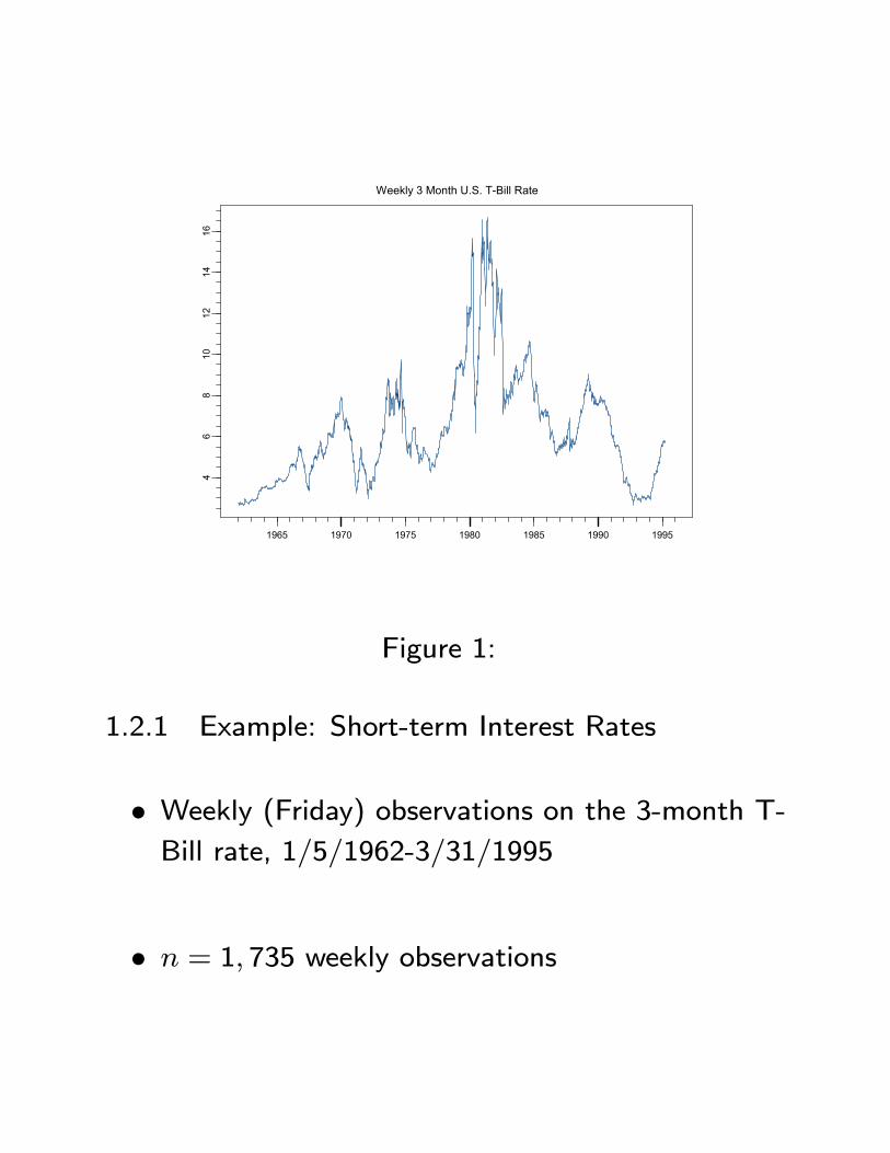
Weekly 3 Month U.S. T-Bill Rate

1965 1970 1975 1980 1985 1990 1995

46

810

1214

16

Figure 1:

1.2.1 Example: Short-term Interest Rates

• Weekly (Friday) observations on the 3-month T-Bill rate, 1/5/1962-3/31/1995

• n = 1, 735 weekly observations

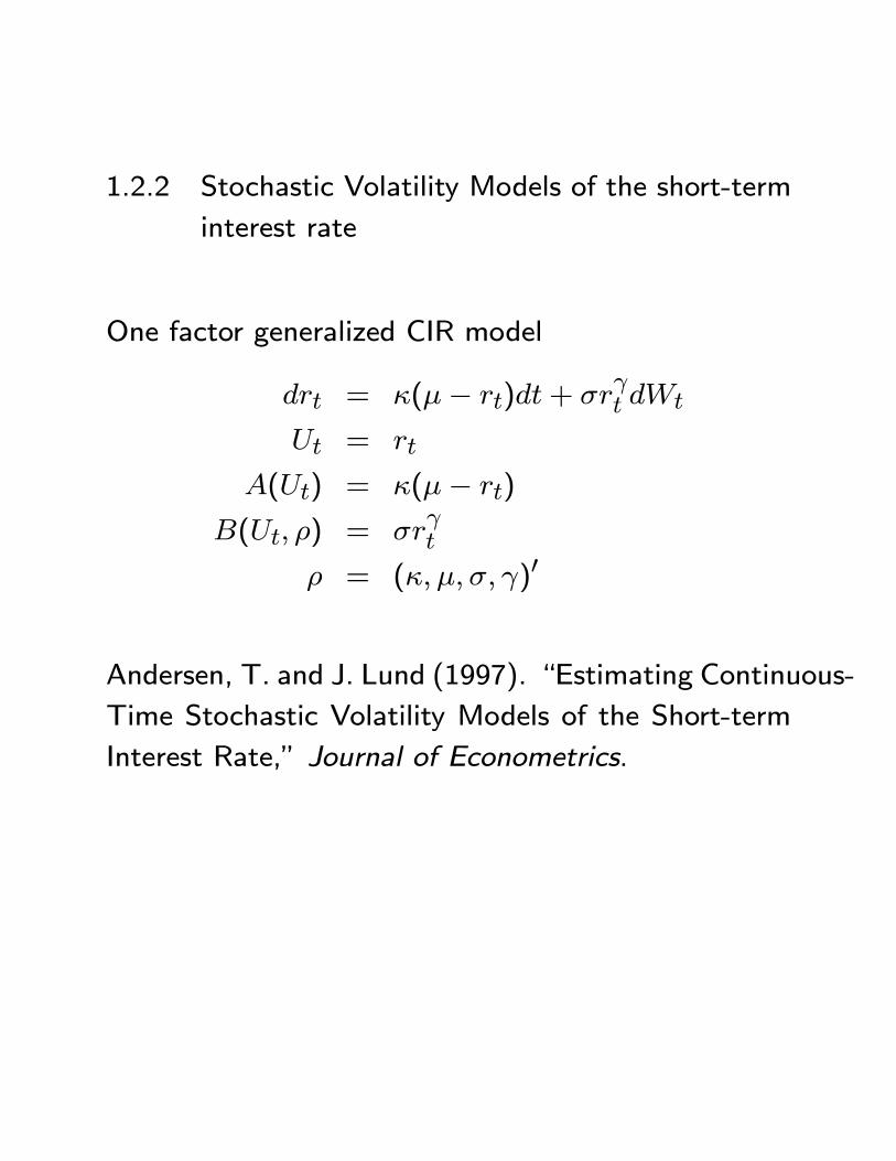
1.2.2 Stochastic Volatility Models of the short-term

interest rate

One factor generalized CIR model

drt = κ(µ− rt)dt+ σrγt dWt

Ut = rt

A(Ut) = κ(µ− rt)

B(Ut, ρ) = σrγt

ρ = (κ, µ, σ, γ)0

Andersen, T. and J. Lund (1997). “Estimating Continuous-

Time Stochastic Volatility Models of the Short-term

Interest Rate,” Journal of Econometrics.

Two factor model

dvt = (av + avvvt + avrrt)dt

+(b1v + b1vvvt + b1vrrt)dW1t + b2vdW2t

drt = (ar + arrrt)dt+ (b2r + b2rrrt) exp(vt)dW2t

where

Ut = (vt, rt)0, Wt = (W1t,W2t)

0

A(Ut, ρ) =

Ãav + avvvt + avrrt

ar + arrrt

!

B(Ut, ρ) =

Ãb1v + b1vvvt + b1vrrt b2v(b2r + b2rrrt) exp(vt) 0

!Identification restrictions

b1vv = 0, b2v = 0, av = −avv

1. Gallant, R. and G. Tauchen (1998). “Reproject-

ing Partially Observed Systems with Application

to Interest Rate Diffusions,” Journal of the Amer-

ican Statistical Association.

1.3 ML and GMM Estimation

yt ∼ iid p(yt|ρ), ρ is L× 1y = (y1, . . . , yn)

0 = random sample

MLE

The MLE for ρ solves

ρmle = argminρ

nXt=1

ln p(yt|ρ)

Equivalently,

0 =nXt=1

∂

∂ρln p(yt|ρmle)

=nXt=1

s(yt|ρmle)

Under regularity conditions, ρmle is consistent and

asymptotically efficient

ρmlep→ ρ0√

n(ρmle − ρ0)d→ N(0, I−10 )

I0 = −E"∂2 ln p(yt|ρ0)

∂ρ∂ρ0

#= E[s(yt|ρ0)s(yt|ρ0)0]

GMM

Suppose there are K ≥ L moment functions

m(yt, ρ) = (m1(yt, ρ), . . . ,mK(yt, ρ))0

such that

Eρ0[m(yt, ρ)] = 0

For example,

m1(yt, ρ) = yt − µ

m2(yt, ρ) = y2t − (σ2 − µ2)

The method of moments estimator of ρ is based on

matching sample moments to population moments,

and solves

mn(ρ) =1

n

nXt=1

m(yt, ρ) = 0

If K > L, there is no solution to the above equation.

For a symmetric and positive definite weight matrix

W, the GMM estimator of ρ solves

ρGMM = argminρ

mn(ρ)0Wmn(ρ)

Under regularity conditions ρGMM is consistent and

asymptotically normally distributed. The efficient GMM

estimator uses a weight matrix that is the inverse of

a consistent estimate of the asymptotic variance of√nmn(ρ0) :

WE = davar(√nmn(ρ0))−1

Remarks:

• The efficient GMM estimator uses the best weight

matrix for a given set of moment conditions.

• A different question is: What are the moment

conditions such that the GMM estimator is effi-

cient in the class of consistent and asymptotically

normal estimators?

Relationship between MLE and GMM

If

mn(ρ) =1

n

nXt=1

s(yt|ρ)

then the GMM estimator is equivalent to MLE. That

is, the best moment conditions to use are based on

the score of the true model.

Remark

The efficient GMM weight matrix in this case is a

consistent estimate of

avar(√nmn(ρ0))

−1 = I−10=³E[s(yt|ρ0)s(yt|ρ0)0]

´−1

1.4 Simulated Method of Moments

Notation

Random Variables : yt, t = −∞, . . . ,∞Data : yi, i = −L, . . . , n

Simulation : yi(ρ), i = −L, . . . , NDummy arguments of summation

(yt−L, . . . , yt−1,yt)yt, xt−1 = (yt−L, . . . , yt−1)

Dummy arguments of integration (put t = 0)

(y−L, . . . , y−1, y0)y = y0, x = (y−L, . . . , y−1)

Assumption underlying the methodology

For ρ in the parameter space, the model generating

the data is presumed to be stationary, ergodic and

convenient to simulate

Consequence

For any lag length L and parameter setting ρ there

exists a stationary density for observables

(yt−L, . . . , yt) ∼ p(y−L, . . . , y0|ρ)And, an unconditional expectation

Eρ£ψ(y−L, . . . , y0)

¤can be computed by generating a long simulation

{yt(ρ)}Nt=−Land averaging

Eρ£ψ(y−L, . . . , y0)

¤ ≈ 1

N

NXt=0

ψ(yt−L(ρ), . . . , yt(ρ))

1.4.1 EMM Estimator

For a quasi-maximum likelihood estimator of an aux-

iliary model with conditional density f(yt|xt−1, θ)

θn = argmaxθ

1

n

nXt=1

ln f(yt|xt−1, θ)

a sample average satisfies

0 =1

n

nXt=1

∂

∂θln f(yt|xt−1, θn),

because these are the first order conditions of the op-

timization problem

Therefore a large simulation from the model with pa-

rametes ρ should satisfy the estimating equations

0 = m(ρ, θn) =1

N

NXt=1

∂

∂θln f(yt(ρ)|xt−1, θn)

except for sampling variation in θn. These estimating

equations hold exactly in the limit as n and N tend

to infinity.

The EMM estimator attempts to find the parameter

vector ρ that solves these estimating equations in a

sense to be made precise below.

1.4.2 Minimum Chi-Squared Estimators

If the equations

m(ρ, θn) = 0

cannot be solved because the dimension of θ is larger

than the dimension of ρ, then

• Use a nonlinear optimizer to solve

ρn = argminρ

m(ρ, θn)0 ³In´−1m(ρ, θn)0³

In´−1

= weight matrix

• In estimates the asymptotic variance of√nm(ρ, θn).If f(y|x, θ) is a good approximation to the truedata generating process p(y|x, ρ0) then an ade-quate estimator is

In = 1

n

NXt=1

·∂

∂θln f(yt|xt−1, θn)

¸ ·∂

∂θln f(yt|xt−1, θn)

¸0Otherwise a HAC estimator of the asymptotic

variance should be used.

1.4.3 Asymptotics

Let ρ0 denote the true value and let θ0 denote an

isolated solution to m(ρ0, θ) = 0. If f(y|x, θ) encom-passes p(y|x, ρ0) , then under regularity conditions

ρnp→ ρ a.s.

√n(ρn − ρ0)

d→ N(0,hM 00I−10 M0

i−1)

where

limn→∞ Mn =M0

limn→∞ In = I0

Mn =M(ρn, θn),M0 =M(ρ0, θ0)

M(ρ, θ) =∂

∂ρ0m(ρ, θ)

I0 = Eρ0

"µ∂

∂θln f(y0|x−1, θ0)

¶µ∂

∂θln f(y0|x−1, θ0)

¶0#Result: The better the auxiliary model approximates

the true structural model, the closer ρn is to the maxi-

mum likelihood estimator based on the true structural

model.

1.4.4 (1− α) · 100% Confidence Intervals

• Wald-type intervalsρi,n ± zα/2 · SE(ρi,n)

SE(ρi,n) =

rhnM 0

nI−1n Mn

i−1ii

Always symmetric - may be misleading

• Invert EMM objective function

qi(ρi) = n · maxρ,ρi fixed

m(ρ, θn)0 ³In´−1m(ρ, θn)0

= profile objective function

{ρi : qi(ρ)− qi(ρi) ≤ χ21−α(1)}Better captures nonlinearity of EMM objective

function

1.4.5 Specification Test and Diagnostics

Under the null hypothesis that p(y−L, . . . , y0|ρ) is thecorrect model

L(ρn, θn) = n ·m(ρn, θn)0³In´−1

m(ρn, θn)0 ∼ χ2(q)

q = dim(θ)− dim(ρ)and

√nm(ρn, θn)

d→ N(0, I0 −M0

hM 00I−10 M0

i−1M 00)

Remarks:

• L(ρn, θn) is the EMM equivalent of the GMM

J−statistic. It is an omnibus statistics for mis-specification. Large values indicate model mis-

specification

• Inspection of the t− ratios

Tn(ρn, θn) = S−1n√nm(ρn, θn)

Sn =·diag(In − Mn

hM 0

nI−1n Mn

i−1M 0

n)¸1/2

can suggest reasons for model failure. Different

elements of the score correspond to different char-

acteristics of the data. Large t− ratios reveal

those characteristics that are not well approxi-

mated.

• The t−ratios Tn(ρn, θn) do not account for un-certainty in ρn and are biased downward (toward

zero). They are therefore conservative.

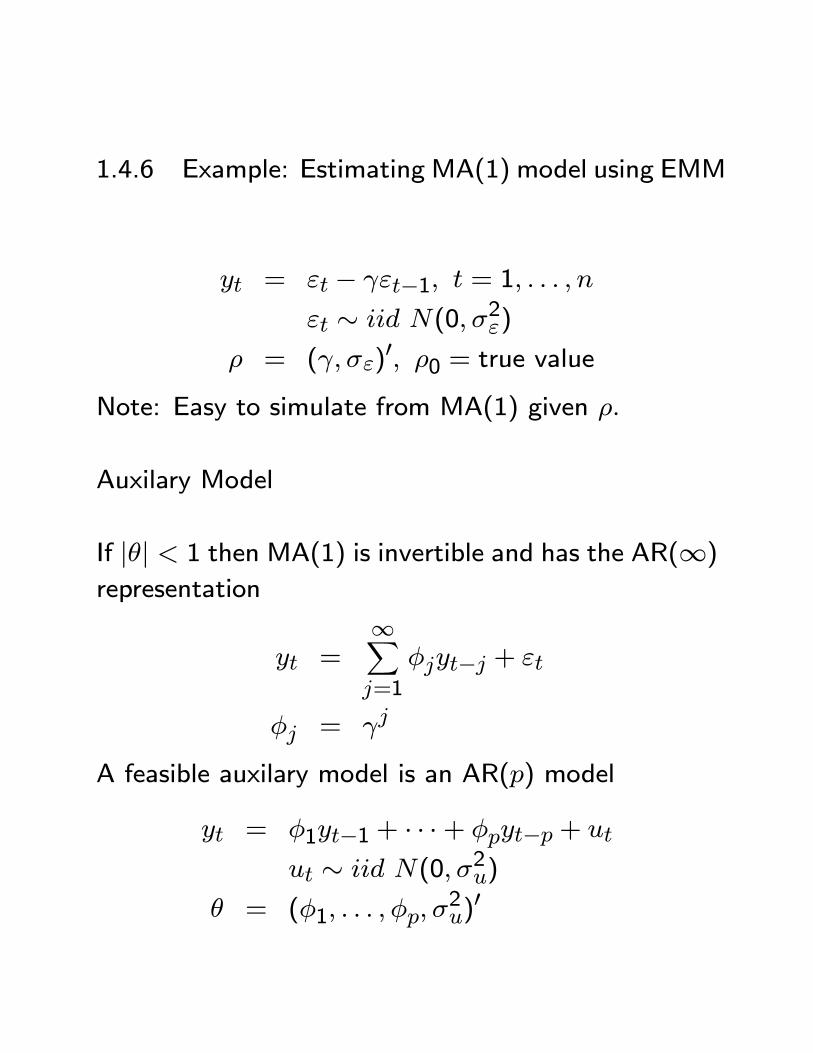
1.4.6 Example: Estimating MA(1) model using EMM

yt = εt − γεt−1, t = 1, . . . , nεt ∼ iid N(0, σ2ε)

ρ = (γ, σε)0, ρ0 = true value

Note: Easy to simulate from MA(1) given ρ.

Auxilary Model

If |θ| < 1 then MA(1) is invertible and has the AR(∞)representation

yt =∞Xj=1

φjyt−j + εt

φj = γj

A feasible auxilary model is an AR(p) model

yt = φ1yt−1 + · · ·+ φpyt−p + ut

ut ∼ iid N(0, σ2u)

θ = (φ1, . . . , φp, σ2u)0

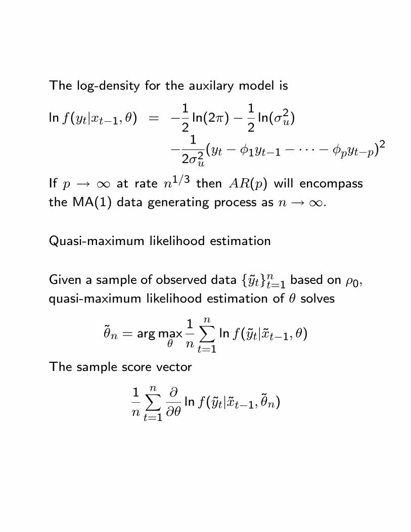
The log-density for the auxilary model is

ln f(yt|xt−1, θ) = −12ln(2π)− 1

2ln(σ2u)

− 1

2σ2u(yt − φ1yt−1 − · · ·− φpyt−p)2

If p → ∞ at rate n1/3 then AR(p) will encompass

the MA(1) data generating process as n→∞.

Quasi-maximum likelihood estimation

Given a sample of observed data {yt}nt=1 based on ρ0,quasi-maximum likelihood estimation of θ solves

θn = argmaxθ

1

n

nXt=1

ln f(yt|xt−1, θ)

The sample score vector

1

n

nXt=1

∂

∂θln f(yt|xt−1, θn)

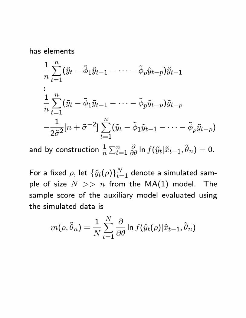
has elements

1

n

nXt=1

(yt − φ1yt−1 − · · ·− φpyt−p)yt−1...1

n

nXt=1

(yt − φ1yt−1 − · · ·− φpyt−p)yt−p

− 1

2σ2[n+ σ−2]

nXt=1

(yt − φ1yt−1 − · · ·− φpyt−p)

and by construction 1n

Pnt=1

∂∂θ ln f(yt|xt−1, θn) = 0.

For a fixed ρ, let {yt(ρ)}Nt=1 denote a simulated sam-ple of size N >> n from the MA(1) model. The

sample score of the auxiliary model evaluated using

the simulated data is

m(ρ, θn) =1

N

NXt=1

∂

∂θln f(yt(ρ)|xt−1, θn)

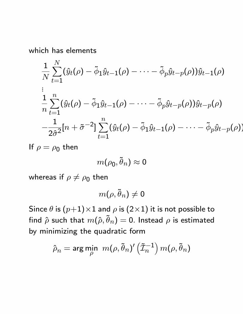
which has elements

1

N

NXt=1

(yt(ρ)− φ1yt−1(ρ)− · · ·− φpyt−p(ρ))yt−1(ρ)

...1

n

nXt=1

(yt(ρ)− φ1yt−1(ρ)− · · ·− φpyt−p(ρ))yt−p(ρ)

− 1

2σ2[n+ σ−2]

nXt=1

(yt(ρ)− φ1yt−1(ρ)− · · ·− φpyt−p(ρ))

If ρ = ρ0 then

m(ρ0, θn) ≈ 0whereas if ρ 6= ρ0 then

m(ρ, θn) 6= 0Since θ is (p+1)×1 and ρ is (2×1) it is not possible tofind ρ such that m(ρ, θn) = 0. Instead ρ is estimated

by minimizing the quadratic form

ρn = argminρm(ρ, θn)

0 ³I−1n ´m(ρ, θn)

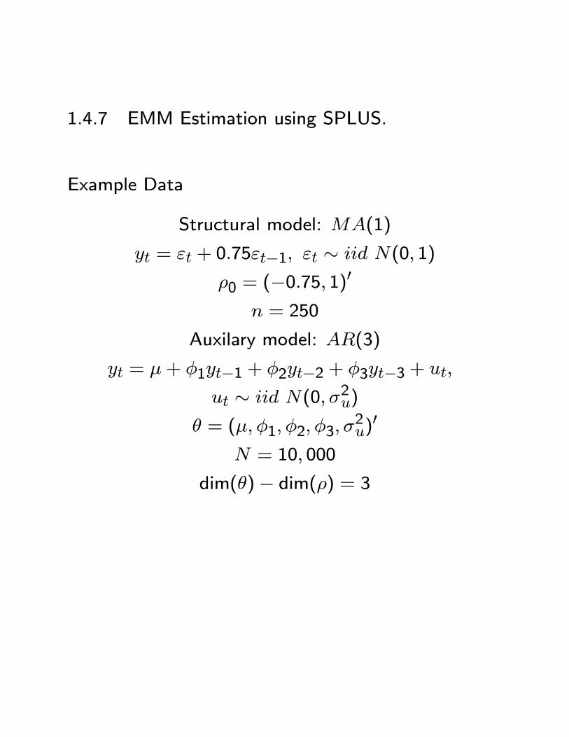
1.4.7 EMM Estimation using SPLUS.

Example Data

Structural model: MA(1)

yt = εt + 0.75εt−1, εt ∼ iid N(0, 1)

ρ0 = (−0.75, 1)0n = 250

Auxilary model: AR(3)

yt = µ+ φ1yt−1 + φ2yt−2 + φ3yt−3 + ut,

ut ∼ iid N(0, σ2u)

θ = (µ, φ1, φ2, φ3, σ2u)0

N = 10, 000

dim(θ)− dim(ρ) = 3

1.5 General Purpose Auxiliary Model: SNP

• SNP is a Semi-NonParametric method, based onan expansion in Hermite functions, for estimation

of the one-step-ahead conditional density f(yt|xt−1, θ).

• It consists of applying classical parametric estima-tion and inference procedures to models derived

from nonparametric truncated series expansions.

• Estimation of SNP models entails using a stan-dard maximum likelihood procedure together with

a model selection strategy that determines the ap-

propriate degree of the nonparametric expansion.

Under reasonable regularity conditions, the esti-

mator is consistent and efficient.

• An important usage of SNP models is to act as ascore generator for EMM estimation.

1.5.1 Assumptions

1. Stationary multivariate data

yt = (y1t, . . . , yMt)0

Stationarity is assumed so that densities for a

stretch of data are time invariant.

2. Markovian structure: the conditional density of

yt given the entire past depend only on a finite

number of lags xt−1 = (yt−L, . . . , yt−1)

3. Smoothness: the density f(yt, xt−1) must havederivatives to the orderML/2 or higher and have

tails that are bounded above by

P (yt−L, . . . , yt) exp12

LXt=0

y2t−L

where P is a polynomial of large but finite degree.

4. Focus is on the estimation of the transition den-

sity

f(yt|xt−1) = f(yt|yt−L, . . . , yt−1)

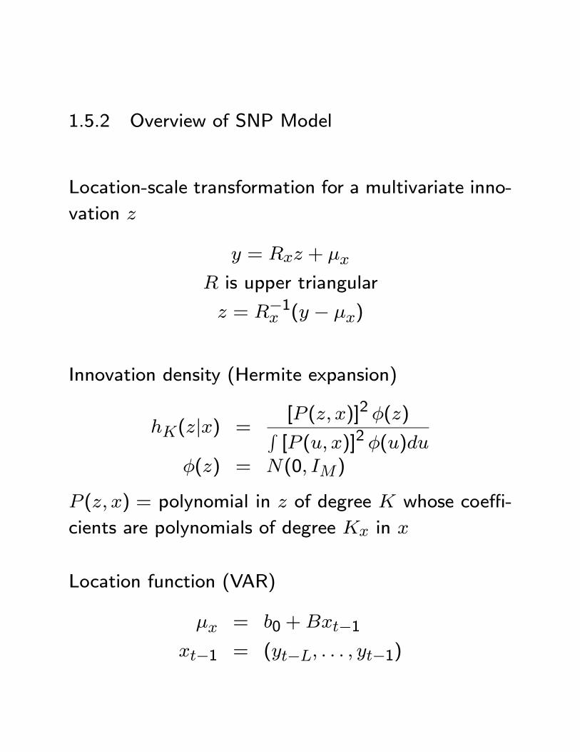
1.5.2 Overview of SNP Model

Location-scale transformation for a multivariate inno-

vation z

y = Rxz + µx

R is upper triangular

z = R−1x (y − µx)

Innovation density (Hermite expansion)

hK(z|x) =[P (z, x)]2 φ(z)R[P (u, x)]2 φ(u)du

φ(z) = N(0, IM)

P (z, x) = polynomial in z of degree K whose coeffi-

cients are polynomials of degree Kx in x

Location function (VAR)

µx = b0 +Bxt−1xt−1 = (yt−L, . . . , yt−1)

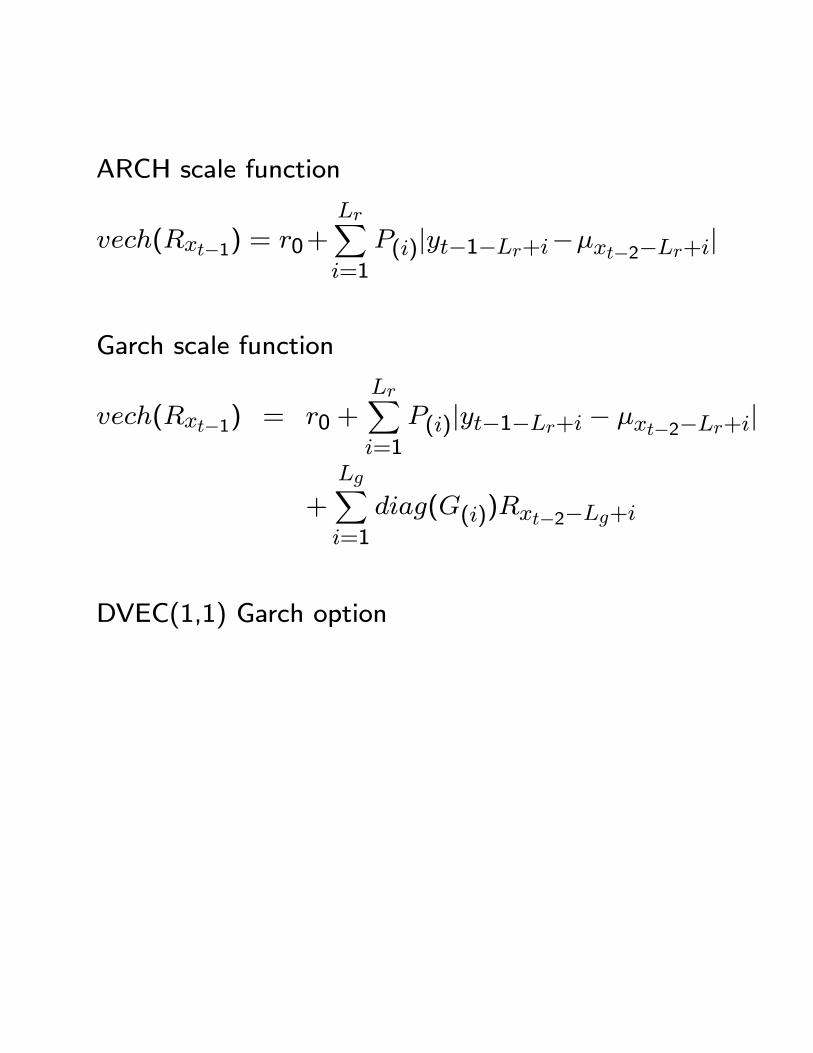
ARCH scale function

vech(Rxt−1) = r0+LrXi=1

P(i)|yt−1−Lr+i−µxt−2−Lr+i|

Garch scale function

vech(Rxt−1) = r0 +LrXi=1

P(i)|yt−1−Lr+i − µxt−2−Lr+i|

+

LgXi=1

diag(G(i))Rxt−2−Lg+i

DVEC(1,1) Garch option

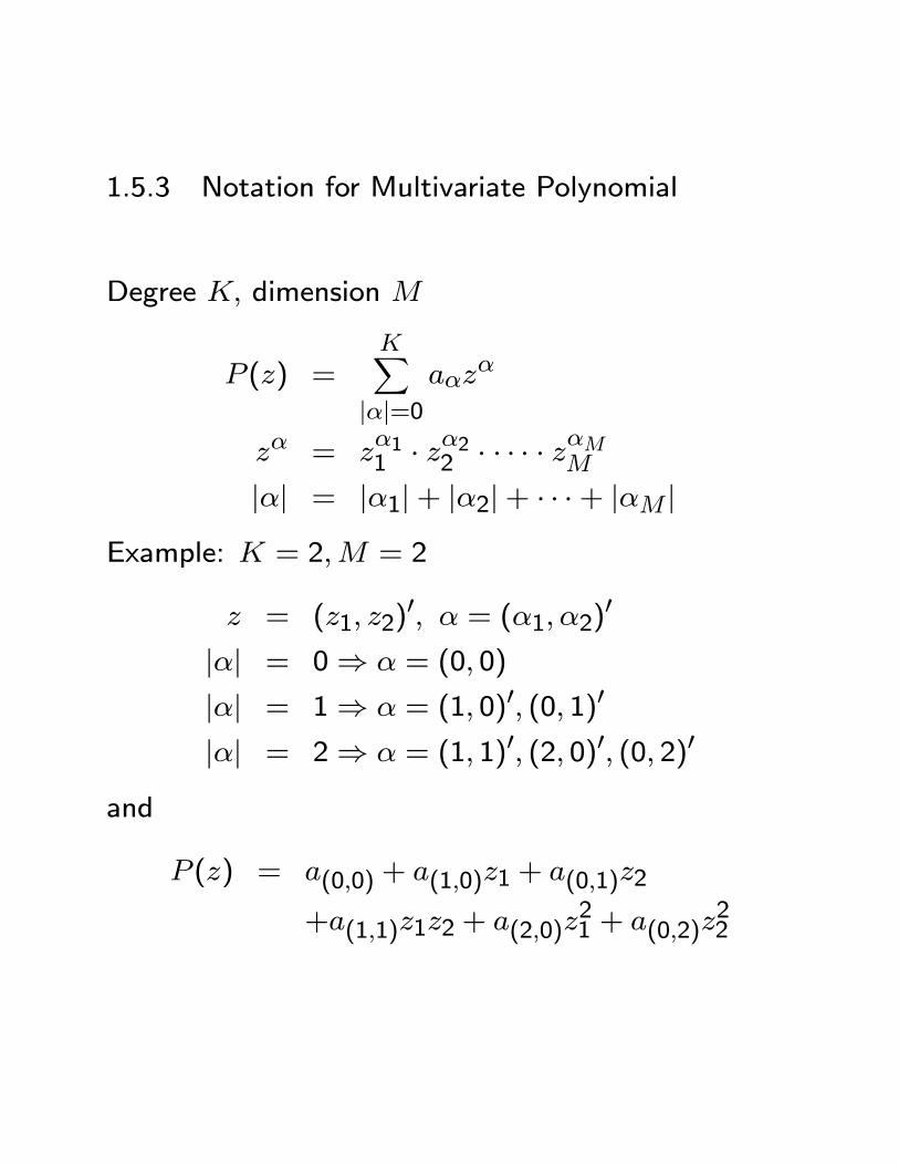
1.5.3 Notation for Multivariate Polynomial

Degree K, dimension M

P (z) =KX

|α|=0aαz

α

zα = zα11 · zα22 · · · · · zαMM

|α| = |α1|+ |α2|+ · · ·+ |αM |Example: K = 2,M = 2

z = (z1, z2)0, α = (α1, α2)0

|α| = 0⇒ α = (0, 0)

|α| = 1⇒ α = (1, 0)0, (0, 1)0

|α| = 2⇒ α = (1, 1)0, (2, 0)0, (0, 2)0

and

P (z) = a(0,0) + a(1,0)z1 + a(0,1)z2

+a(1,1)z1z2 + a(2,0)z21 + a(0,2)z

22

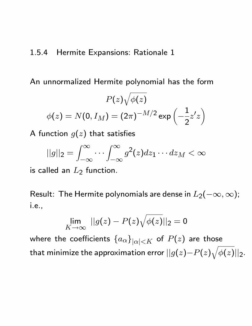
1.5.4 Hermite Expansions: Rationale 1

An unnormalized Hermite polynomial has the form

P (z)qφ(z)

φ(z) = N(0, IM) = (2π)−M/2 exp

µ−12z0z

¶A function g(z) that satisfies

||g||2 =Z ∞−∞

· · ·Z ∞−∞

g2(z)dz1 · · · dzM <∞is called an L2 function.

Result: The Hermite polynomials are dense in L2(−∞,∞);i.e.,

limK→∞ ||g(z)− P (z)

qφ(z)||2 = 0

where the coefficients {aα}|α|<K of P (z) are those

that minimize the approximation error ||g(z)−P (z)qφ(z)||2.

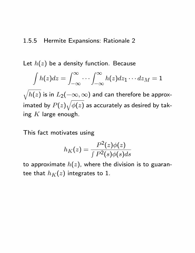
1.5.5 Hermite Expansions: Rationale 2

Let h(z) be a density function. BecauseZh(z)dz =

Z ∞−∞

· · ·Z ∞−∞

h(z)dz1 · · · dzM = 1qh(z) is in L2(−∞,∞) and can therefore be approx-

imated by P (z)qφ(z) as accurately as desired by tak-

ing K large enough.

This fact motivates using

hK(z) =P 2(z)φ(z)RP 2(s)φ(s)ds

to approximate h(z), where the division is to guaran-

tee that hK(z) integrates to 1.

1.5.6 The Main Idea

Take h(z) as the parent density and use a location-

scale transform

y = Rz + µ

to generate a location-scale family of densities

f(y|θ) =nP [R−1(y − µ)]

o2φ[R−1(y − µ)]

| det(R)| R P 2(s)φ(s)dswhich can be estimated from data {yt}nt=1 by quasimaximum likelihood

θ = argmaxθ

nYt=1

f(yt|θ)

The density estimate is

f(y) = f(y|θ)The consistency of the estimator was established by

Gallant and Nychka (1987), “Semi-Nonparametric Max-

imum Likelihood Estimation,” Econometrica.

1.5.7 SNP Density: iid Data

Location-scale transform

y = Rz + µ, z = R−1(y − µ)

R = upper triangular

Density

f(y|θ) ∝ P 2[R−1(y − µ)] ·N(y|µ,Σ)Σ = RR0

Example: K = 2, M = 2

R =

ÃR11 R120 R22

!θ = (a(0,0), a(1,0), a(0,1),

a(1,1), a(2,0), a(0,2),

µ1, µ2, R11, R12, R22)

a(0,0) = 1 (normalization)

How well does SNP do at approximating densities?

• SNP performs well relative to kernel estimators

• SNP performs well on the Marron andWand (1992)test suite densities.

References

1. Fenton, V.M. and R. Gallant (1996). Conver-

gence Rates of SNP Density Estimators, Econo-

metrica.

2. Fenton, V.M. and R. Gallant (1996). Qualitative

and Asymptotic Performance of SNP Density Es-

timators, Journal of Econometrics.

1.5.8 Choice of K

Results in Coppejans and Gallant (2000), “Cross Val-

idated SNP Density Estimates,” indicate that mini-

mizing the BIC seems to work well for determining

the degree K of the polynomial P (z)

Estimation: Eqivalent to maximum likelihood, but

more numerically stable is to minimize the negative

of the average log likelihood

θn = argminθ

sn(θ)

sn(θ) = −1n

nXt=1

ln f(yt|θ)

Schwarz criterion (BIC): Choose K to minimize

BIC(p) = sn(θ) +p

2nln(n)

p = number of free parameters in θ

1.5.9 SNP Transition Density for Time Series

The idea is to modify the location and scale trans-forms of the SNP density for iid data to be functionsof the past, which is the standard method of modify-ing a model for iid data for application to time seriesdata. Lastly, the SNP density itself is modified to ac-comodate non-homogeneous innovations. The stepsare as follows.

VAR location function:

y = Rz + µxt−1µxt−1 = b0 +Bxt−1xt−1 = (yt−Lu, . . . , yt−1)

0Lu = VAR order

b0 is M × 1, B is M × Lu.

Density

f(y|θ) ∝ P 2[R−1(y − µxt−1)] ·N(y|µ,RR0)Kz = 0⇒ Gaussian VAR

Kz > 0⇒ non-Gaussian VAR

ARCH-type scale function

y = Rxt−1z + µxt−1µxt−1 = b0 +Bxt−1

vech(Rxt−1) = r0 +LrXi=1

P(i)|yt−1−Lr+i − µxt−2−Lr+i|Lr = ARCH order

where

r0 is M(M + 1)/2× 1P = [P(1)| · · · |P(Lr)] is M(M + 1)/2× Lr

Density

f(y|θ) ∝ P 2[R−1xt−1(y − µxt−1)] ·N(y|µ,Rxt−1R0xt−1)

Kz = 0, Lr > 0⇒ Gaussian VAR-ARCH

Kz > 0, Lr > 0⇒ non-Gaussian VAR-ARCH

GARCH-type scale function

y = Rxt−1z + µxt−1µxt−1 = b0 +Bxt−1

vech(Rxt−1) = r0 +LrXi=1

P(i)|yt−1−Lr+i − µxt−2−Lr+i|

+

LgXi=1

diag(G(i))Rxt−2−Lg+i

Lg = ARCH order

where

G = [G(1)| · · · |G(Lg)] is M(M + 1)/2× Lg

Density

f(y|θ) ∝ P 2[R−1xt−1(y − µxt−1)] ·N(y|µ,Rxt−1R0xt−1)

Kz = 0, Lg > 0⇒ Gaussian VAR-GARCH

Kz > 0, Lr > 0⇒ non-Gaussian VAR-GARCH

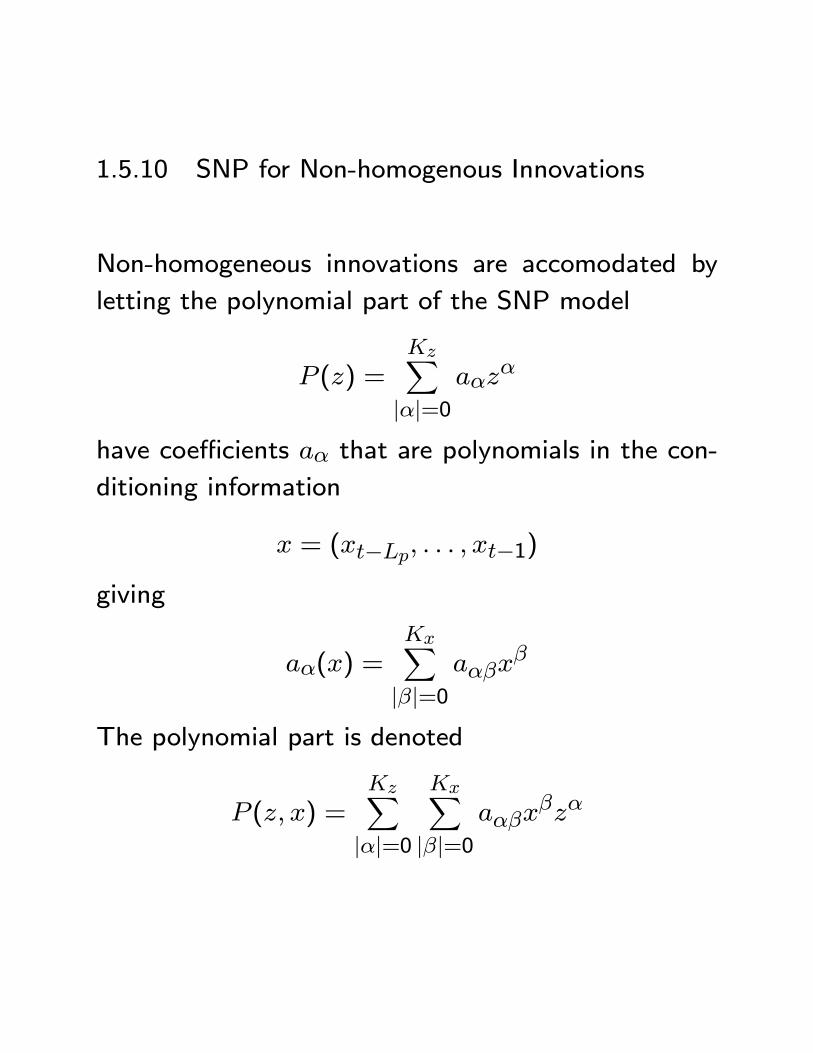
1.5.10 SNP for Non-homogenous Innovations

Non-homogeneous innovations are accomodated by

letting the polynomial part of the SNP model

P (z) =KzX|α|=0

aαzα

have coefficients aα that are polynomials in the con-

ditioning information

x = (xt−Lp, . . . , xt−1)

giving

aα(x) =KxX|β|=0

aαβxβ

The polynomial part is denoted

P (z, x) =KzX|α|=0

KxX|β|=0

aαβxβzα

The SNP density for the non-homogeneous innova-

tions is a Hermite polynomial in z whose coefficients

are polynomials in x

hK(z|x) =P (z, x)φ(z)RP (s, x)φ(s)ds

K = (Kz,Kx)0

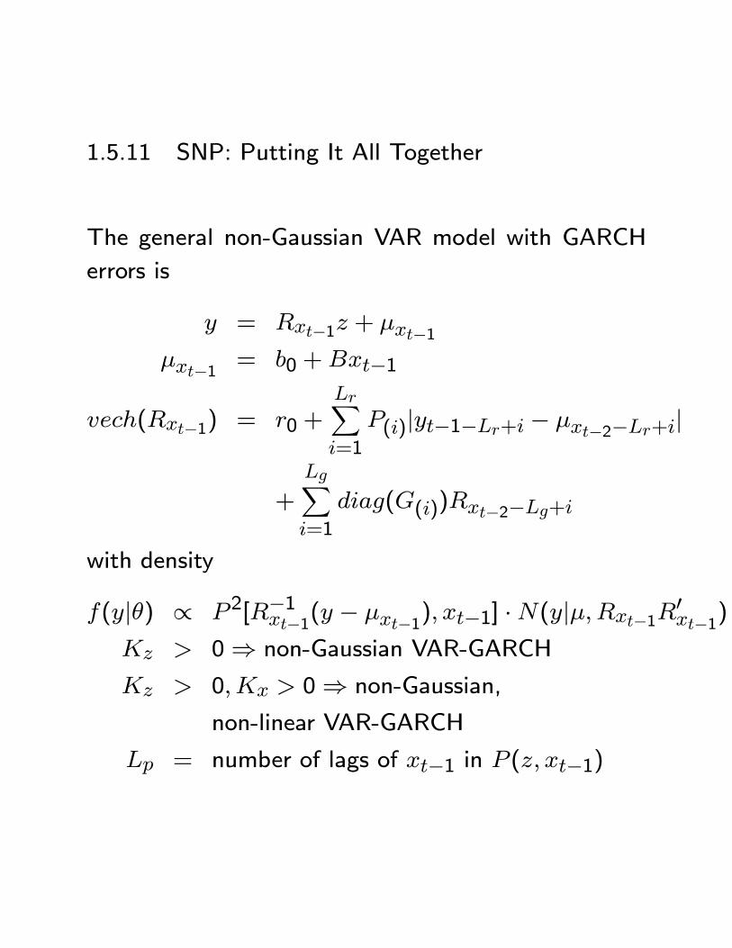
1.5.11 SNP: Putting It All Together

The general non-Gaussian VAR model with GARCH

errors is

y = Rxt−1z + µxt−1µxt−1 = b0 +Bxt−1

vech(Rxt−1) = r0 +LrXi=1

P(i)|yt−1−Lr+i − µxt−2−Lr+i|

+

LgXi=1

diag(G(i))Rxt−2−Lg+i

with density

f(y|θ) ∝ P 2[R−1xt−1(y − µxt−1), xt−1] ·N(y|µ,Rxt−1R0xt−1)

Kz > 0⇒ non-Gaussian VAR-GARCH

Kz > 0,Kx > 0⇒ non-Gaussian,

non-linear VAR-GARCH

Lp = number of lags of xt−1 in P (z, xt−1)

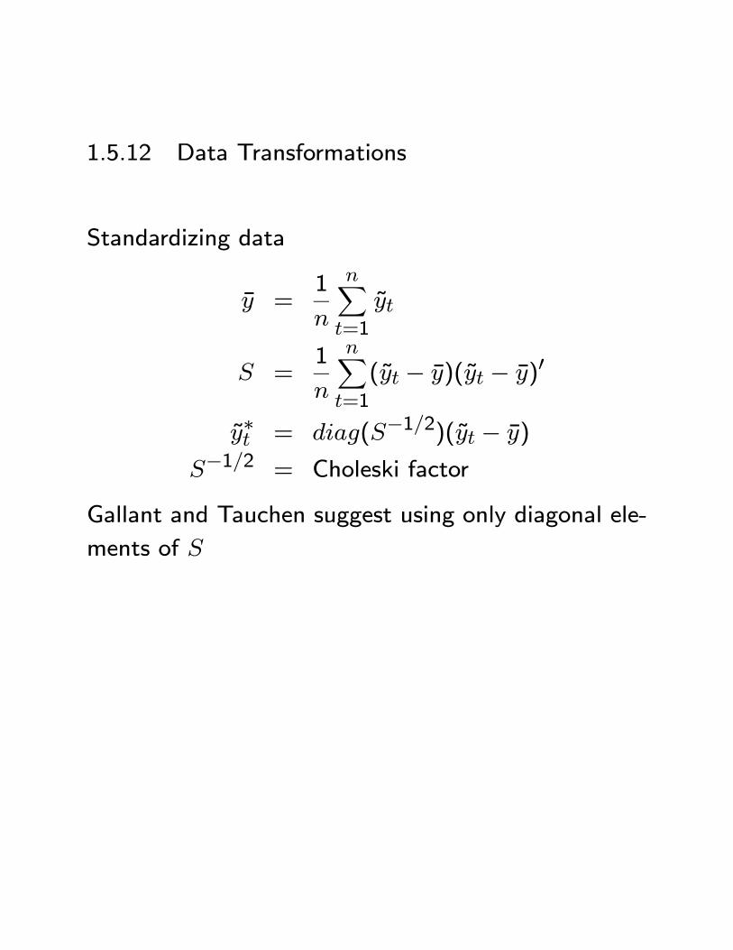
1.5.12 Data Transformations

Standardizing data

y =1

n

nXt=1

yt

S =1

n

nXt=1

(yt − y)(yt − y)0

y∗t = diag(S−1/2)(yt − y)

S−1/2 = Choleski factor

Gallant and Tauchen suggest using only diagonal ele-

ments of S

Adjusting for extreme values in xt−1

Problem: If the ture density f(y|x) is heavy tailed,then xt−1 will contain extreme observations, whichhave a strong and undesirable influence on estimates

when Lr > 0 (ARCH terms). Additionally, if data

are highly persistent (like interest rates), fitted SNP

models can generate explosive simulations

Cure: Replace each component of x by its log spline

transform

x∗i =

12 [xi − σtr − ln(1− xi − σtr)] xi < −σtr

xt −σtr ≤ xi ≤ σtr12 [xi + σtr + ln(1− σtr + xi)] σtr < xi

σtr = 4

Note: Spline transformation attenuates potential ex-

plosive simulations yt(ρ) that may occur during course

of EMM estimation

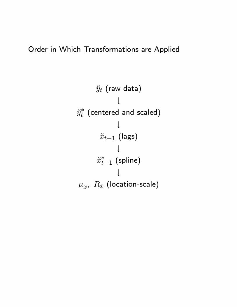
Order in Which Transformations are Applied

yt (raw data)

↓y∗t (centered and scaled)

↓xt−1 (lags)

↓x∗t−1 (spline)

↓µx, Rx (location-scale)

1.5.13 Asymptotics

If the parameters of f(y|x, θ) are estimated by quasi-maximum likelihood

θn = argminθ

sn(θ)

sn(θ) = −1n

nXt=1

ln f(yt|xt−1, θ)

and K = (Kz,Kx)0 grows with the sample size, thenthe estimator

fn(y|x) = f(y|x, θ)converges almost surely to the true transition density

f(y|x) in Sobolev norm as n→∞. Moreover, K can

depend on the data.

Reference:

Gallant, R. and D. Nychka (1987). “Seminonparamet-

ric Maximum Likelihood Estimation,” Econometrica.

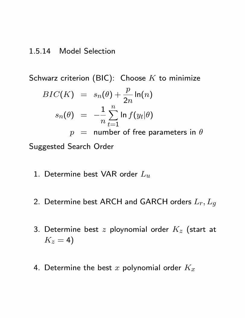
1.5.14 Model Selection

Schwarz criterion (BIC): Choose K to minimize

BIC(K) = sn(θ) +p

2nln(n)

sn(θ) = −1n

nXt=1

ln f(yt|θ)p = number of free parameters in θ

Suggested Search Order

1. Determine best VAR order Lu

2. Determine best ARCH and GARCH orders Lr, Lg

3. Determine best z ploynomial order Kz (start at

Kz = 4)

4. Determine the best x polynomial order Kx

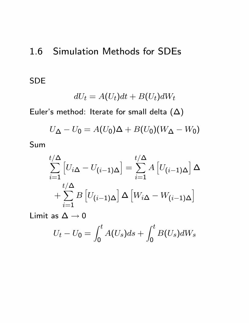
1.6 Simulation Methods for SDEs

SDE

dUt = A(Ut)dt+B(Ut)dWt

Euler’s method: Iterate for small delta (∆)

U∆ − U0 = A(U0)∆+B(U0)(W∆ −W0)

Sum

t/∆Xi=1

hUi∆ − U(i−1)∆

i=

t/∆Xi=1

AhU(i−1)∆

i∆

+t/∆Xi=1

BhU(i−1)∆

i∆hWi∆ −W(i−1)∆

iLimit as ∆→ 0

Ut − U0 =Z t

0A(Us)ds+

Z t

0B(Us)dWs

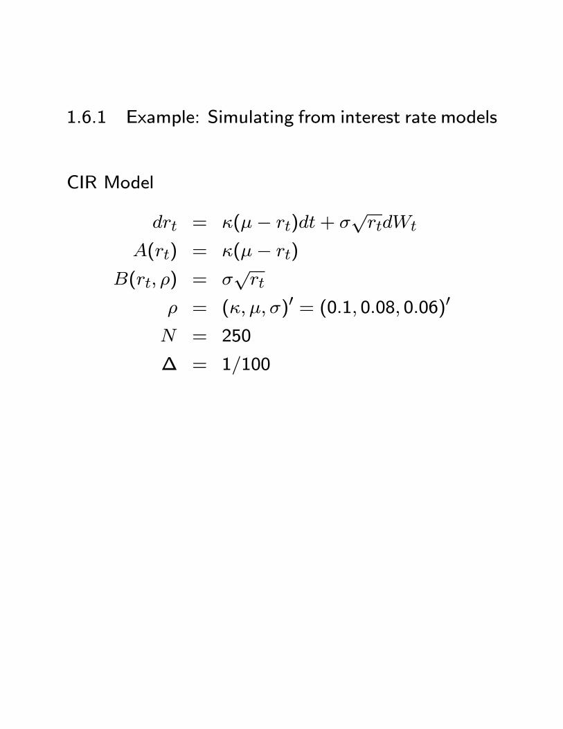
1.6.1 Example: Simulating from interest rate models

CIR Model

drt = κ(µ− rt)dt+ σ√rtdWt

A(rt) = κ(µ− rt)

B(rt, ρ) = σ√rt

ρ = (κ, µ, σ)0 = (0.1, 0.08, 0.06)0

N = 250

∆ = 1/100

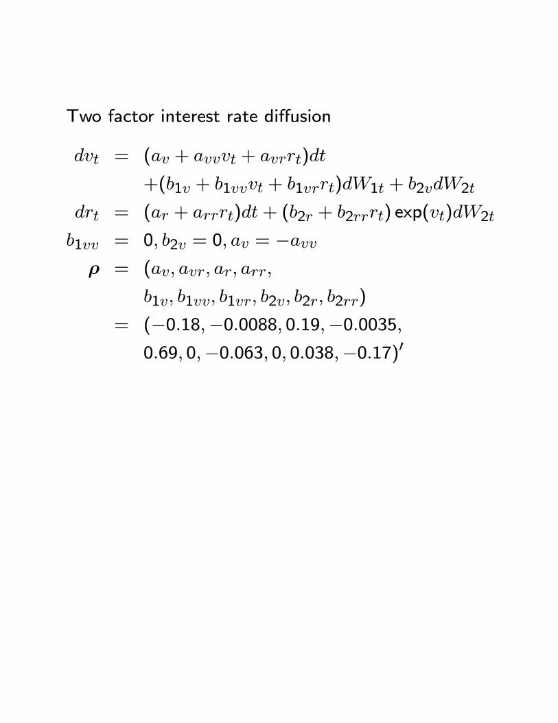
Two factor interest rate diffusion

dvt = (av + avvvt + avrrt)dt

+(b1v + b1vvvt + b1vrrt)dW1t + b2vdW2t

drt = (ar + arrrt)dt+ (b2r + b2rrrt) exp(vt)dW2t

b1vv = 0, b2v = 0, av = −avvρ = (av, avr, ar, arr,

b1v, b1vv, b1vr, b2v, b2r, b2rr)

= (−0.18,−0.0088, 0.19,−0.0035,0.69, 0,−0.063, 0, 0.038,−0.17)0

1.7 EMM Estimation of Continuous Time

Models for Interest Rates

1. Fit SNP Model to observed data

2. Create simulator functon for continuous time model

3. Estimate model by EMM

4. Check EMM diagnostics