simulation methods for estimation of blocking
TRANSCRIPT

Simulation Methods for Estimation of BlockingProbabilities in Cellular Telecommunication Networks
Felisa J. Vazquez-Abad∗
Department of Computer Science and Operations Research
University of Montreal, Montreal, Canada H3C 3J7
Email: [email protected]
also Principal Fellow, Department of Electrical and Electronic Engineering
The University of Melbourne
Lachlan L. H. Andrew †
ARC Special Research Centre for Ultra-Broadband Information Networks
Department of Electrical and Electronic Engineering
The University of Melbourne, Victoria 3010, Australia
Email: [email protected]
January 5, 2001CUBIN Technical Report 2001-01-01
∗Supported in part by NSERC-Canada grant # WFA0184198†Supported by the Australian Research Council (ARC).
1

Contents
1 Introduction 3
2 Blocking Probabilities 5
3 Fast Simulation Methods 83.1 Relative Ef"ciency . . . . . . . . . . . . . . . . . . . . . . . . . . . . . . . . 83.2 Rare Events . . . . . . . . . . . . . . . . . . . . . . . . . . . . . . . . . . . . 93.3 Importance Sampling and BRE . . . . . . . . . . . . . . . . . . . . . . . . . . 103.4 Large Deviations and Asymptotic Optimality . . . . . . . . . . . . . . . . . . 12
4 Estimation of Closed Form Probabilities 144.1 Acceptance/Rejection Method . . . . . . . . . . . . . . . . . . . . . . . . . . 154.2 Markov Chain Monte Carlo Methods . . . . . . . . . . . . . . . . . . . . . . . 174.3 Numerical Results . . . . . . . . . . . . . . . . . . . . . . . . . . . . . . . . . 19
5 Model for Fast Simulation 22
6 Static ISSC Estimation for Light Traffic 256.1 Change of Measure . . . . . . . . . . . . . . . . . . . . . . . . . . . . . . . . 256.2 Numerical Results . . . . . . . . . . . . . . . . . . . . . . . . . . . . . . . . . 27
7 Dynamic ISSC Estimation for High Capacity 297.1 Change of Measure . . . . . . . . . . . . . . . . . . . . . . . . . . . . . . . . 297.2 Implementation considerations . . . . . . . . . . . . . . . . . . . . . . . . . . 31
7.2.1 Subsampling the ribs . . . . . . . . . . . . . . . . . . . . . . . . . . . 317.2.2 Choice of quasi-regenerative cycles . . . . . . . . . . . . . . . . . . . 32
7.3 Simulation results . . . . . . . . . . . . . . . . . . . . . . . . . . . . . . . . . 33
8 Concluding Remarks 34
A Estimating Variance 37
2

Abstract
Blocking probabilities in FDMA/TDMA cellular mobile communication networks us-ing dynamic channel assignment are hard to compute for realistic sized systems. Thiscomputational dif"culty is due to the structure of the state space, which imposes strongcoupling constraints amongst components of the occupancy vector. Tractable models fordynamically recon"gurable networks have been proposed, and for those, the stationarydistribution of the occupancy vector is a product of truncated Poisson random variables.Nonetheless, even in such cases realistic network sizes prevent computation of the closedform within reasonable time and the only viable way to estimate blocking seems to bethrough simulation.
Alas! Simulation as a means for estimating blocking probability suffers from the factthat the relative error of the estimates can grow without bound for the same number of sam-ples, as the blocking probability diminishes. Small blocking probabilities thus typicallyrequire an enormous amount of CPU time for the estimates to be meaningful. Advancedsimulation approaches use importance sampling (IS) to overcome this problem. This isknown in the simulation literature as rare event simulation.
Two simulation approaches can be identi"ed. The "rst one attempts to use simula-tion as a means for generating the stationary distribution directly. We review the Accep-tance/Rejection (A/R) method and a fast simulation approach applied to it. While it doesgive a remarkable variance reduction, this method requires solving a complex optimisationproblem before IS can be applied. Next we describe a Markov Chain Monte Carlo methodthat we have call the Filtered Gibbs Sampler (FGS), which dramatically outperforms A/Rand does not need any set-up to perform the simulations.
The second simulation method is to simulate the actual occupancy process and estimateblocking from the measurements. This method can in principle be more robust than estima-tion of the product form probabilities, because realistic channel assignments can be dealtwith, and not just models that satisfy the product form. In this paper we study two regimesunder which blocking is a rare event: low utilisation and high capacity. Our simulationsuse the Standard Clock (SC) method that generates directly the birth and death process andwe propose a change of measure that we call static ISSCwhich has bounded relative error:as the traf"c intensity decreases, the relative ef"ciency of this method becomes in"nitelybetter than the FGS method. For high capacity, we use a change of measure that dependson the current state of the network occupancy. This is the dynamic ISSCmethod, for whichwe can prove optimality in single clique models and we empirically show the advantagesof this method over na1ve simulation for networks of moderate size and traf"c loads.
1 Introduction
Ef"cient design of communications networks requires the ability to determine the quality ofservice provided by a particular network con"guration. A common quality of service mea-sure is the blocking probability, which is the probability that a new call will not be admittedto the network due to insuf"cient network resources. This paper will consider techniques fordetermining the blocking probability in cellular telephony systems with frequency reuse, in-cluding "rst generation systems such as the Advanced Mobile Phone System, AMPS (Lee,1995), and second generation systems such as the Global System for Mobile communication,GSM (Mouly and Pautet, 1992, Redl, Weber, and Oliphant, 1995).
3

In cellular networks, each mobile station communicates with a base station connected to thewireline telephone network. The region in which mobiles connect to a given station is calleda cell. Each mobile station communicates with its base station using a speci"c frequency pairor frequency/timeslot pair known as a channel. To avoid interference, this channel cannotbe used in nearby cells; however, it may be reused in cells suf"ciently remote that interferencecaused by the reused channel is below a speci"ed threshold.
In static assignment schemes, each cell is allocated a "xed subset of the available channels,and calls arriving in a cell are connected only when there are free channels available fromthose channels. While simple to implement, this strategy may result in wasted resources: allthe channels for one cell may be in use, but adjacent cells may have free capacity that couldbe used to connect incoming calls without causing interference. Network capacity can beimproved by dynamic channel assignment(Cox and Reudink, 1972, Cox and Reudink, 1973),in which channels not
currently in use in the nearby cells may be used. It is these systems which are the focus ofthis paper.
Many techniques have been developed for determining the performance of such networks.For Markov models (Poisson arrivals and exponential holding times), when the system is re-versible (Kelly, 1979), the stationary state distribution has a simple product form expressionon a state space S which is a small subset of a hypercube H . When there is no mobility ofusers, this is the case under maximum packing (Everitt and Macfadyen, 1983 and see below),in which calls in progress can be rearranged. There are also models of mobility which preservethis property (see Pallant and Taylor (1995), Boucherie and Mandjes (1998)). Moreover, theresult remains valid even when call holding times have non-exponential distributions (Kelly,1979).
The product form expression involves a normalising constant, from which the blockingprobability can be determined directly, without needing to determine speci"c state probabil-ities. However, it is computationally prohibitive to calculate explicitly for large systems.Product form systems have been studied extensively (see for example the survey of Nelson(1993)). When the number of channels is large but the number of cells is small, it can besolved exactly by recursive methods (Dziong and Roberts, 1987, Pinsky and Conway, 1992),mean value analysis (Reiser and Lavenberg, 1980), generating function inversion
methods (Choudhury, Leung, andWhitt, 1995) or uniform asymptotic approximation (MitraandMorrison, 1994). However, these techniques all have exponential complexity in the numberof cells.
Systems with a large number of cells can be analysed by Monte Carlo techniques, either toestimate the normalising constant (Ross and Wang, 1992 or to avoid the need to calculate it.The simplest approach of the second type is acceptance/rejection (A/R) method, in which statesare generated in the full hypercubeH: those lying outside the state space S are rejected, whilefor those on the boundary of the feasible region, the proportion of blocked cells is recorded(see for example Everitt and Macfadyen, 1983). As the number of cells grows, generation ofa sample point inside the state space S ⊂ H may become a rare event, and so importancesampling has been applied to these methods (see Ross, Tsang, and Wang, 1994, Lassila andVirtamo, 2000, Mandjes, 1997). An alternative approach is to use Markov chain Monte Carlo(MCMC) techniques such as the Gibbs sampler used by Vazquez-Abad and Andrew (2000),Lassila and Virtamo (1998a) and Lassila and Virtamo (1998b). These generate a Markov chainwhose state probabilities satisfy the target product form, and they may be simulated more
4

ef"ciently.Most dynamic channel assignment implementations do not have such a product form solu-
tion. It is common in such cases is to use closed form approximations, such as the ubiquitousreduced load approximation Kelly, 1991, developed for circuit switched networks. This ap-proximation works well if there is minimal correlation between blocking due to con#icts withdifferent reuse constraints, but poorly if there is signi"cant correlation. Due to the spatial na-ture of the reuse constraints in the cellular case, it can be expected that there will be signi"cantcorrelation. Other approximations are described in Harvey and Hills (1979) and Zahorjan,Eager, and Sweillam (1988).
A very #exible, straightforward and hence common approach is simply to simulate thedirect arrival and departure process of calls. This allows any parameters of the system tobe measured, and allows arbitrary channel allocation schemes to be compared directly. Forthese reasons, this is the approach most commonly taken by engineers investigating differentdynamic channel assignment systems. However, this approach can be very slow, especiallywhen blocking rates are low. Then the method is not suitable for the dimensioning of large realworld networks. In this paper, we present two importance sampling schemes for the ef"cientdirect simulation of systems with low blocking probabilities.
2 Blocking Probabilities
A cellular network is a surface in a two-dimensional space that is covered by a partition of Ksubsets (called cells). Each cell has a base station that supports C channels, each of whichallows one user to communicate with the base station. The principle behind cellular networksis that the limited number of channels available can be reused across the network, provided thatthe so-called reuse constraints are satis"ed. These constraints ensure that the performance inany given cell is not excessively degraded by the interference caused by other cells using thesame channel elsewhere. The reuse constraints hence depend on the precise
layout of the cells. For the examples in this paper, we shall assume that the cells form ahexagonal grid and 3-cell reuse is employed. That is, the reuse constraints are that no channelmay be used more than once in any group of three mutually adjacent cells. In general, a set ofcells in which a channel may only be used once is called a clique. Figure 1 shows a simpleseven-cell network, with one clique highlighted.
1
2
3
4
5
6
7
Figure 1: Simple cellular network model
5

Calls can arrive at the cell in one of two ways. They may be new calls or they may beexisting calls being handed off from neighbouring cells due to user mobility. Using dynamicchannel assignment, calls arriving to a cell are assigned one of the available channels. If nochannel can be allocated without violating a reuse constraint, then the call is blocked. Other-wise it is accepted, and uses the selected channel. In practice, the call will generally use thesame channel until it leaves the cell. Thus in general the state of the system depends not onlyon the number of calls in each cell, but also on which particular channels they use.
Let K be the number of cells in the network, M be the number of cliques, and C be thenumber of channels. Let cj be the jth clique, j = 1, . . . ,M . For the seven cell network ofFigure 1, cj : j = 1, . . . ,M = (1, 2, 3), (1, 3, 4), (1, 4, 5), (1, 5, 6), (1, 6, 7), (1, 2, 7).
When the channel assignment cannot be changed while a call is in progress, very little canbe said about the occupancy of cell i in the states when blocking occurs, except that it must ofcourse be less than C. In particular, it is possible for calls to be blocked when there are no callsat all in cell i, if all the channels are used elsewhere in the cliques to which i belongs. However,since some channels may be used in one clique and some in another, there is not even a usefullower bound on the number of calls in any of the individual cliques containing i. De"ne thecluster associated with cell i to be the union of all cliques containing i:
Ci =⋃cj3i
cj.
It is then possible to say that the occupancy of the clusterCi must be at least C when callsarriving to cell i are blocked, since each channel must be blocked by at least one of the cliquescontaining cell i. This is the fundamental property of blocking states on which the methodspresented here rely.
Most of the techniques described in the introduction rely on having a known closed form forthe blocking probability. There is such a closed form for the maximum packing bound proposedby Everitt and Macfadyen (1983), in which channels may be reassigned on the arrival of a newcall. However, the operation of reassigning calls is not feasible in practice, and so this closedform does not apply to real channel assignment algorithms. The techniques presented later onin Sections 6 and 7 are applicable to real channel assignment algorithms and are thus of moregeneral applicability than most of the techniques described in the introduction. However, itwill simplify the description to describe the algorithm initially for the maximum packing case.This removes the dependence on which particular channels are occupied; the behaviour of thesystem is determined entirely by the number of calls in each cell. Moreover, we will make theclique packing approximation of Everitt and Macfadyen (1983), Raymond (1991), which onlyconsiders constraints local to each clique.
Under clique packing, a state is feasible if eachof the cliques contains no more calls thanthere are channels:
n(cj) ≤ C ∀j = 1, . . . ,M (1)
where n(A) is the number of calls in a set of cells, A, in a given network state, n.In general, the state of the process is n(t) = (n1,1(t), . . . , nK,C(t)), where n(i, j)(t) = 1
if channel j is used in cell i at time t, and zero otherwise. Under maximum packing, this canbe simpli"ed to n(t) = (n1(t), . . . , nK(t)), where ni(t) represents the number of channels inuse at cell i at time t, At each cell i calls arrive following independent Poisson process with
6

corresponding intensities λi, i = 1, . . . , K. Upon arrival of a call at cell i at time t, it is acceptedif there is still at least one channel available. Under maximum packing, the requirement is that
maxcj3i
(n(cj)) ≤ C − 1.
An accepted call on channel j causes ni,j(t) = ni,j(t−)+1 (ni(t) = ni(t
−)+1 under maximumpacking), all other components of the state remaining unchanged. We say that at this time thecall is
connected. If an incoming call to cell i "nds no channels available (under maximum pack-ing, the current state satis"es (1) with equality for some cj 3 i) then all channels are used andthe call is blocked, with no change to the state.
Calls stay connected for a random length of time called the holding time, assumed to beexponentially distributed and independent of the rest of the process history. All holding timesare identically distributed with mean 1/µ. When a call using a channel on cell i terminates, thecorresponding occupancy component is decreased by one unit. Although the holding times areassumed to be exponential in this paper, the network performance is in fact independent of theholding time distribution for many channel assignment schemes, including maximum packing(Kelly, 1979). This model gives rise to a continuous-time Markov process.
Because the process consists of independent arrivals and departures, it may be expectedthat it is a form of birth and death process. Indeed it can be expressed as a quasi birth anddeath(QBD) process (Neuts, 1981). In QBD processes, states can be arranged in layers, suchthat transitions from layer n can only be to states in layers n − 1, n or n + 1. If the nth layerconsists of states in which a cluster Ci contains n calls, then the system is clearly a QBD, sincea call arrival within the cluster causes a transition from layer n to layer n + 1, a departurewithin the cluster causes a transition from n to n − 1, and an arrival or departure outside thecluster causes a transition entirely within level n. In this representation, all blocking states arein layers C or higher.
Let S be the state space consisting of all integer vectors n = (n1, . . . , nK) ∈ NK satisfying(1). The process can be seen as a truncated multidimensional birth and death process for eachcomponent: a particular case of a QBD where the rates and barriers depend on all componentsof the process. When the process is in state n ∈ S, the birth rate of component i is λi1n6∈Bi,where 1A is the indicator function of event A and the set Bi is the set of blocking states forcell i, that is:
Bi = n ∈ S : ∃cj 3 i, n(cj) = C, i = 1, . . . , K (2)
The death rate at cell i in state n ∈ S is niµ.The performance measure of interest is called the blocking probability, and it is de"ned as
the long term probability that an incoming arrival is lost:
B = limt→∞
∑Ki=1 Yi(t)
A(t)=
K∑i=1
(λiλ
)Bi =
K∑i=1
(λiλ
)π(Bi) (3)
where Yi(t) is the total number of calls lost in cell i up to time t and A(t) is the total numberof arrivals up to time t. The term Bi is the long term proportion of calls arriving to cell i thatare blocked, and π(Bi) is the stationary probability that the state is in the blocking set Bi.
Evaluating blocking probabilities using (3) is a dif"cult numerical problem. Everitt andMacfadyen (1983) propose a methodology that identi"es geometrical structures corresponding
7

to the cliques within the network and characterizes the constraint sets in terms of the geometryof the cells. This is used to calculate the normalization factor G(C), where the sums have torespect (1). This method for calculating blocking probabilities is computationally prohibitivewhen the number of cells is large, which means that simulation is often superior.
The renewal theorem can be used to re-write (3) in terms of expectations within regenerativecycles. However, as the system state has many components, regeneration cycles are frequentlytoo long to be a feasible basis for simulation. The concept of quasi-regenerationwas introducedto calculate stationary averages for such systems, as explained in Gaivoronski and Messina(1996) and Chang, Heidelberger, and Shahabuddin (1995). Consider a random process, n, andassume it starts with the stationary distribution P[n(0) = n] = π(n). Consider a set of points,A, such that there is an a.s. "nite stopping time T1 de"ned as the "rst entry time to the setA from its complement A′ and such that the distribution of the process n(t + T1); t > 0is identical to that of the process n(t); t > 0 with n(0) ∈ A drawn from the stationarydistribution of the process, conditioned on being on the boundary of the set A. The set A iscalled a quasi-regenerative set. Because the channel occupancy process n(t) described above isan irreducible Markovian process on a "nite state space, all subsets of the state space are quasi-regenerative sets and a unique stationary measure π exists. The times between consecutiveentries to the set A are termed A-cycles. Unlike true regenerative cycles, A-cycles may notbe independent, but they are still identically distributed.
It will be useful to consider different quasi-regeneration sets, Ai, for different cells i. LetT (i) be the time of the "rst reentry to set Ai, and Xi(T
(i)) be the amount of time within anAi-cycle that the process spends in Bi. Then (Breiman, 1992)
Bi =E[Xi(T
(i))]
E(T (i)). (4)
The sets Ai will be chosen in such a way as to minimise the required simulation time.
3 Fast Simulation Methods
3.1 Relative Efficiency
To approximate the value ofB, simulation can be used to produce a sample of random variablesYs, s = 1, . . . , S whose sample average is consistent for B, namely,
E[Y (S)] =1
S
S∑s=1
E[Ys]→ B
as S →∞. In some cases Y (S) is unbiased, that is, E[Y (S)] = B. When consecutive samplescome from independent replicas of a simulation, the variance of Y (S) can easily be estimated.Under some conditions on the boundedness of this variance, Alexopoulos and Seila (1998)show that the Central Limit Theorem (CLT) holds:
Y (S)−BVar[Y (S)]
L=⇒N (0, 1)
8

whereL
=⇒ represents convergence in distribution andN (0, 1) is the standard normal distribu-tion. Con"dence intervals (see Larson, 1973) can then be approximated using:
limS→∞
P
B 6∈ Y (S)± z(1−α/2)
√Var[Y (S)]
≤ α,
where z1−α/2 is the upper (1 − α/2) quantile of the normal distribution. In order to achieve aprespeci"ed precision within a
con"dence level α, S must be large enough for Var[Y (S)] to be within the speci"ed limits.Some estimators have less variance than others, yet they may require extremely long simulationtimes. A commonly used measure which takes this into account (see for example Glynn andWhitt, 1992) is that of the efficiencyof an estimator. When estimating probabilities, one oftenrequires estimating the probabilities within a given relative error, in terms of a percentage ofthe (unknown) probability. In these cases, the sample size must grow in order for√
Var[Y (S)]
B
to remain at the required level.
Definition 1 Therelative ef"ciency of a consistent estimatorY (S) is:
Er(Y (S)) =B2
CPU[Y (S)]Var[Y (S)], (5)
whereCPU[Y (S)] denotes the average CPU time of the simulation that produces theS samples.Theasymptotic relative ef"ciency is defined aslimS→∞ Er(Y (S)), if this limit exists.
In particular, if the simulation has produced a sample of i.i.d. random variables, then therelative ef"ciency is independent of S: CPU times tend to grow linearly with the sample sizeand Var[Y (S)] decreases as 1/S. When estimating ef"ciencies, we shall often use the esti-mated values of B and of Var[Y (S)] in the de"nition of Er. If the estimators are known notto be consistent, i.e., limS→∞ E[Y (S)] 6= B, then the actual de"nitions of ef"ciency use themean square errors instead of the variances. In this paper we deal with consistent or unbiasedestimation, so the problem of estimating the MSE is not present.
In this paper we will compare several simulation methods for estimating B, in terms oftheir ef"ciencies.
3.2 Rare Events
The occupancy process n(t); t ≥ 0, as described in Section 2 is a continuous time Markovprocess on (Ω,P) referring to a truncated birth and death process with state-dependent re#ect-ing boundaries. The arrival rate of calls into cell i is λi, i = 1, . . . , K, and the average holdingtime per call is 1/µ.
Fix any cell i and consider expression (4) of the blocking probability Bi using A-cycles.Then T (i) is the duration of an A-cycle, which is adapted to the natural filtrationof the processn(t); t > 0; that is, knowledge of the process history up to time t is suf"cient to determine
9

if the A-cycle terminates at this epoch, and note that T (i) must necessarily coincide with anarrival to one of the cliques where cell i belongs.
De"ne now τi to be the stopping time when blocking states are reached and Ri to be theevent that the occupancy process enters the blocking set Bi before the cycle is over:
τi = mink : Sk ≤ T (i) and n(Sk) ∈ Bi, and Ri = Sτi < T (i). (6)
Equation (4) requires estimation of the proportion of time that the process spends in block-ing states. For all ω with 1Ri(ω) = 0, Xi(T
(i))(ω) = 0, thus the numerator in (4) can beestimated with:
E[Xi(T(i))] = E
(E[Xi(T
(i))|Ri] 1Ri).
Definition 2 Letn(t) be a process defined on a probability space(Ω, Fk, k ≥ 0,P) and letε > 0 be a parameter of the distribution of the processn(t). Denote byPε the correspondingdistribution. The eventR ⊂ Ω is called arare event if limε→0 Pε(R) = 0.
EXAMPLE: In the cellular network problem, Ri is a rare event under several different param-eterizations. In particular, if λi(ε) → 0 as ε → 0, then the blocking probability tends to zero.We will study this light traf"c regime. As well, it is of importance to study the case whenC → ∞, where C is the maximum number of available channels in the cellular network. An-other high capacity regime, GI/G/s queues with buffer size C has been thoroughly studied(see for example Sadowsky, 1991), but the methods for that system are not applicable to ourcase.
÷×÷×÷×If p(ε) = Pε(Ri) is estimated via simulation using 1Ri for S consecutive A-cycles, then
the variance of the estimator is at least p(ε)(1−p(ε))/S because consecutiveA-cycles introducepositive correlation on the Bernoulli sequence. The relative error in the estimation is boundedbelow by: √
p(ε)(1− p(ε))/Sp(ε)
≈√
(1− p(ε))S p(ε)
→∞
as ε → 0. Larger and larger sample sizes S must be used to obtain the same accuracy in theestimation for different parameter values. The ef"ciency in the estimation of rare events can beimproved using a change of measure approach via importance sampling (see Bratley, Fox, andSchrage, 1987, Asmussen and Nielsen, 1995, and Devetsikiotis and Townsend, 1993 amongothers).
3.3 Importance Sampling and BRE
Assume an underlying Markovian process Uk with natural "ltration Fk = σ(U1, . . . , Uk),such that the occupancy process n(t) can be embedded into a discrete event process
adapted to the "ltration Fk, k = 1, 2, . . .. Use the notation n(k), k = 1, 2, . . . for theembedded process (with the obvious abuse in notation).
EXAMPLE:Discrete event simulation is commonly performed by generating, for each cell, the inter-
arrival times Ak(i), k = 1, 2, . . . according to a Poisson process with rate λi, and the holding
10

times Hk(i), k = 1, 2, . . . as independent exponential variables with mean 1/µ. At the arrivalepochs to cell i, given by the expression:
St(i) =t∑
k=1
Ak(i),
the occupancy process ni increases by one, provided n 6∈ Bi. At the call termination epochsSk(i)+Hk(i) the corresponding component decreases by one. Identify Uk(i) = (Ak(i), Hk(i)).Then the embedded process is adapted to the "ltration Fk = σ(U1(i), . . . , Uk(i)(i); i = 1, . . . , K),where k(i) is the number of arrivals occurring at cell i amongst the "rst k total arrivals.
÷×÷×÷×The general structure of the evolution of the Markovian process Uk is assumed to satisfy:
P[Uk+1 ∈ A|Fk] = P[Uk+1 ∈ A|n(k)]. In the example above, Uk+1 is actually independent ofthe state n(k); the more general formulation will prove useful for the standard clock techniquein Section 5.3. Let fn(u) be the conditional density of Uk+1 given the state n(k) = n (the casewhere Uk has discrete components can be treated in a similar way). Then for any real valuedfunctional of the process Ψ(U1, U2, . . .) with "nite expectation, and any "nite integer T ,
E[Ψ(U1, . . . , UT )] =
∫Ψ(u1, . . . , uT )
[T−1∏k=0
fn(k)(uk+1)
]du1, . . . duT , n0 : initial state.
Let now f∗n(·) be anotherconditional density. Multiplying and dividing each term in the prod-uct above by the new densities, we obtain:
E[Ψ(U1, . . . , UT )] =
∫Ψ(u1, . . . , uk)
(T−1∏k=0
fn(k)(uk+1)
f ∗n(k)(uk+1)
)[T−1∏k=0
f ∗n(k)(uk+1)
]du1, . . . duk
= E∗[Ψ(U1, . . . , UT )L(U1, . . . , UT )];
L(U1, . . . , UT ) =T−1∏k=0
fn(k)(Uk+1)
f ∗n(k)(Uk+1)≡ LT (7)
where E∗ denotes the expectation w.r.t. a different probability: here the process Ukevolves according to the transition densities f ∗. When Lk is interpreted as a statistics depend-ing on the observations, it is called the likelihood ratio. The above expression is valid forgeneral functionals only when the support of the old distributions is contained within that of thenew distributions, i.e., if for every u > 0, fn(u) > 0 implies f ∗n(u) > 0 for the correspondingdensities. In such cases one says that the original measure P is absolutely continuousw.r.t. P∗,denoted by P << P∗. In the case of rare event estimation for the cell blocking probability,we will identify T = τi and Ψ = 1Ri. The change of measure approach can be specializedto the important region and (7) can be used for densities such that P∗(Ri) is as close to 1as desired, even if P is not absolutely continuous w.r.t. P∗, as long as PcRi is, where PcRithe restriction of P to the important set Ri (see Vazquez-Abad and LeQuoc, 2001). In thiscase the Radon-Nikodym derivative is no longer called a likelihood ratio, but it still satis"esE[1Ri] = E∗[Lτi1Ri].
Remark: The random process Lk, k = 1, 2 . . . is what is known as a (multiplicative)P∗-martingale adapted to the "ltration, because it satis"es E∗[Lk+1|Fk] = Lk. This martingale
11
de"nes the appropriate Radon-Nikodym derivative for functionals of the process Uk, andthe change of measure (7) is valid also when T is a stopping time, which is a consequence ofWald's identity, as explained in detail in Asmussen and Nielsen (1995), Sadowsky (1991).
Definition 3 An unbiased IS estimator for the rare event probabilityP(Ri) = p(ε), E∗[Lτi1Ri]has asymptoticbounded relative error (BRE) if there are constantsb <∞, ε0 > 0 such that:
supε≤ε0
√Var∗[Lτi1Ri]
E∗[Lτi1Ri]≤ b. (8)
It is usually desirable to "nd a new probability P∗ such thatP∗(Ri) → 1 as ε → 0, with Lτi1Ri ≤ 1 w.p.1. for all ε. It is in this sense that the
estimation can be performed faster and with variance reduction. Indeed, the variance of theestimator without IS is Var(1Ri) = p(ε)[1− p(ε)], but under the new measure,
Var∗(Lτi1Ri) = E∗[L2τi1Ri]− p2(ε) = E[Lτi1Ri]− p2(ε) ≤ p(ε)− p2(ε),
because (7) can be applied to Ψ = Lτi and we have assumed that Lτi1Ri ≤ 1 w.p.1. Thefollowing lemma is a direct consequence of De"nition 3.
Lemma 1 If there are constantsd1, d2 and b such thatp(ε) ≥ d1εb andL1R ≤ d2ε
b a.s.,then the IS estimatorL1R is BRE forp(ε).
3.4 Large Deviations and Asymptotic Optimality
By construction, under any change of measure with bounded Radon-Nikodym derivative itholds that p(ε) = Pε(R) = E∗[L1R]. Often the new measure depends on ε, and L will ingeneral also be a function of ε, although we will not make this explicit in our notation. Becausevariances are non negative, it must always be true that:
E∗[L2 1R] ≥ p2(ε). (9)
Estimators that satisfy (9) with equality are optimal.
Definition 4 Suppose that there is a constantv and a functionh(v, ε) such thath(v, ε)→ 0 asε→ 0, at a rate which increases with increasingv, and
limε→0
h−1(p(ε), ε) = v,
whereh−1(p, ·) is the inverse ofh(v, ·) with respect to the first argument, so thath−1(h(v, ε), ε) =v. An IS estimator ofp(ε) is is said to beasymptotically optimal (a.o) if it satisfies:
limε→0
h−1(√
E∗[L2 1R], ε)
= v. (10)
In particular, if the rare event probability is exponentially decreasing, p(ε) ≈ e−v/ε, thenh(v, ε) = e−v/ε and h−1(p, ε) = −ε log(p). If the rare event probability is geometricallydecreasing, p(ε) ≈ εv, then h(v, ε) = εv and h−1(p, ε) = log(p)/ log(ε).
It follows that a BRE estimator of rare event probability will be asymptotically optimal.
12

Definition 5 For a distributionF (·), theexponentially twisted distribution is defined by:
dF (α)(x) =e−αx
M(−α)dF (x) = e−αx−Γ(α)dF (x),
whereM(α) = E[eαX ] is the moment generating function (MGF) ofF andΓ(α) = log(M(−α))is correspondingly called the log-MGF.
In the case that exponential twisting is used for a change of measure, the likelihood ratiois given by L(X) = eαX+Γ(α). In many known problems, exponential twisting can yield BREand asymptotically optimal estimators.
EXAMPLE: The model is a GI/G/s/∞ queueing system: s parallel servers with in"nitequeueing capacity. Interarrival times Ai are i.i.d. following a distribution FA with log-MGFΓA(α) and all services are i.i.d. with distribution FB with log-MGF ΓB(α). Sadowsky (1991)shows the large deviations result for the over#ow probability:
limn→∞
1
nlog p(n) = ΓA(sα∗),
where p(n) is the probability that the queue size will reach n customers in waiting within eachA-cycle, and α∗ satis"es ΓA(sα∗)+ΓB(−α∗) = 0. Sadowsky uses the following de"nition: thestart of an A-cycle is the arrival time of a customer that "nds s− 1 servers busy. Let the initialdistribution of the s residual service times H(i)
0 , i = 1, . . . , s be the stationary distribution atthe start of the A-cycle. For the Markovian model all residual service times are exponentiallydistributed. De"ne T as the index of the next customer that "nds again s−1 servers busy. Nextde"ne τ as the index of the "rst customer that "nds n customers in the queue. Necessarily, allthe s servers must be busy at this time and other n customers wait in queue. This implies thaton the set τ < T , for each server i:
Ni(τ)∑k=0
H(i)k < Sτ ≤
Ni(τ)+1∑k=0
H(i)k , (11)
whereH(i)k are the consecutive service times at server i andNk(i) are the number of customers
that have departed from server i by the time of the k-th arrival. Furthermore, because at timeSτ there are still n customers waiting, then necessarily:
s∑i=1
Ni(τ)+1∑k=0
H(i)k =
τ−n∑k=0
Hk
where Hk is the service time of the k-th customer (regardless of which server it goes to).
Theorem 1 (Sadowsky)The IS estimator obtained using the exponentially twisted measuresF ∗A(x) = F sα∗
A (x), F ∗B(y) = F(−α∗)B (y) is the only asymptotically optimal IS estimator.
Consider the "ltration of the process Ft = σ((Ak, Hk); k = 0, . . . , t), and notice that knowl-edge of the interarrival and service requirements is suf"cient to determine which server is
13

assigned to each customer (FCFS). Using independence between Ai, Hi, under the proposedchange of measure, the Radon-Nikodym derivative is the adapted process:
Lt =t∏
k=0
e−sα∗Ak+ΓA(−sα∗) eα
∗Hk+ΓB(α∗)
which, evaluated at time τ , can be re-written as:
Lτ1τ<T = exp
α∗s∑i=1
Sτ − Ni(τ)+1∑k=0
H(i)k
− α∗ τ∑k=τ−n+1
Hk
= exp
−α∗
(s∑i=1
H(s)0 +
τ∑k=τ−n+1
Hk
),
where H(i)0 is the residual service time at server i at the time of the τ arrival Sτ . For the
exponential model, these are simply the exponentials. For Poisson arrivals, these would havethe stationary distribution at a full busy cycle. Call R(s, α∗) = log
∏i E∗[eα
∗H(i)0 ] its log-
MGF and assume that it is bounded (as would be in the case of exponential residual times).By assumption, the service times of the customers in queue are independent of these residualtimes (under the original as well as the star measure). We will use the fact that under thenew measure, over#ow is asymptotically certain, that is, P∗(R) → 1 as n → ∞. The largedeviations rate can be calculated using:
p(n) = E∗[Lτ 1R] = E∗[Lτ |1R]P∗(R)→ eR(s,α∗)[E∗(e−α∗H1)]n = eR(s,α∗)+nΓA(sα∗),
where we have used that (Hk; k = τ − n, . . . , n) are i.i.d. independent of τ . The last identityis a consequence of the de"nition of the conjugate twisted exponentials:
E∗[e−α∗Hk+ΓB(−α∗)−ΓB(−α∗)] = e−ΓB(α∗) = eΓA(sα∗).
It is now straightforward to evaluate limn→∞1n
log p(n).In the special case of an M/M/s/∞ server, where FA(·) ∼ exp(λ), FB(·) ∼ exp(µ) the
conjugate exponential twisting yields:
MA(α) = E[eαA1] =λ
λ− α, F(α)A ∼ exp(λ− α), α > −λ
α∗ =sµ− λs
, F ∗A ∼ exp(sµ), F ∗B ∼ exp(λ/s),
and it is known as rate swapping: one again simulates an M/M/s/∞ server, with the newrates:
λ∗ = sµ, µ∗ = λ/s. (12)
In Sections 6 and 7 we discuss the implementation of the IS that swaps arrival and servicerates for the cellular network problem.
÷×÷×÷×
14
4 Estimation of Closed Form Probabilities
This section presents two methods for estimating blocking probabilities by means of (3), whenthe channel assignment model satis"es the product form solution. In particular, for the maxi-mum packing model, the stationary cell occupancy probability is a truncated multivariate Pois-son distribution
(Boucherie and Mandjes, 1998, Everitt and Macfadyen, 1983)
π(n) =1
G(C)
K∏i=1
(ρniini!
), n ∈ S (13)
where ρi = λi/µ is the offered traf"c to cell i, and
G(C) =∑n∈S
K∏i=1
(ρniini!
)is the normalizing constant. This section studies the estimation of the blocking probabilities in(3) by generating a sample of random variables Xs ∈ S with distribution π(·) to calculate:
B =K∑i=1
(λiλ
)π(Bi).
4.1 Acceptance/Rejection Method
The method of acceptance/rejection explained in Ross (1997) and Bratley, Fox, and Schrage(1987) is used for generating random variables. In the case of truncated distributions, it is anatural method of generating a random variable n with the stationary probability π(n) of (13).The method follows the recursion:
Algorithm 1: A/R
1. Repeat
(a) GenerateM1, . . . ,MK independent variables withMi ∼Poisson(ρi).
Until N = (M1, . . . ,MK) ∈ S
2. Xs = N
3. s← s+ 1, go to 1.
The resulting random variables Xs have distribution π in (13).This method is used in Everitt and Macfadyen (1983) and Yates (1997) to calculate (3) as
follows. Random variables Xs are generated according to Algorithm 1. Next, compute:
Ys =K∑i=1
(λiλ
)1Xs∈Bi (14)
15

which identi"es for which cells the state Xs is in a blocking state and weights the probabilityaccordingly. By de"nition, Bi ∩ Bj 6= ∅ for i 6= j, and this overlapping means that some statesmay block several adjacent cells. By construction, Ys is an unbiased estimator of the blockingprobability: E[Ys] = B. Clearly the samples Ys, s = 1, . . . , S are independent, and the CLTcan be used to build con"dence intervals (35) for the estimation.
The acceptance probability G(C) can be very low for moderately large networks. Tosee this, imagine the feasible region of the seven-cell network projected on (ni, ni+1, ni−1)as shown in Figure 2.
ni-1
ni+1
ni
Tetrahedron Hypercube of side length C
of edges of length C- n1
Figure 2: Projection of the feasibility region S.
For each value of n1 ≤ C a tetrahedron contained in the hypercube of side length C sym-bolizes the feasible region on the projected coordinates. Clearly other coordinates will be alsoconstrained by the values of ni−1 and ni+1. Even if a pre-calculated table is used to generatePoisson random variables truncated to the hypercube, that is, Mi ∼Poisson(ρi)cC ,Mi ≤ Ca.s., the volume of the feasible region can be considerably smaller than the whole space. Thissuggests the use of IS as follows (refer to Section 6.2).
EXAMPLE: The canonical large deviations example deals with sample averages, as in Boucherieand Mandjes (1998), Bucklew (1990). Suppose that Sn =
∑ni=1 Xi where Xi, i = 1, 2, . . . are
zero-mean i.i.d. random variables with well de"ned MGFM(α). The rare eventR = Sn/n >a, for a > 0 is exponentially decreasing with increasing n, and it is well known that:
limn→∞
1
nlog P[Sn/n > a] = −α∗ a+ Γ(−α∗) ≡ −v(a),
where α∗ satis"es α∗ a − Γ(α∗) = supα∈R(α a − Γ(α)). The rate of convergence is clearlythe same as the exponent of the likelihood ratio for the exponential twisting with parameter α∗.Using this change of measure for each Xi, by independence the Radon-Nikodym derivative is:
L(X1, . . . , Xn) =n∏i=1
e−α∗Xi+Γ(−α∗) = e−α
∗Sn+nΓ(−α∗)
16

so that logL1R ≤ −α∗(na) + nΓ(−α∗), where we have used 1R = Sn ≥ na. Non-negativity of the variance implies that
1
nlog E∗[L21R] ≥ −2v(a), as n→∞.
Identifying ε = 1/n, it then follows that this change of measure yields an asymptoticallyoptimal IS estimator.
Boucherie and Mandjes (1998) and Mandjes (1997) use a scaling large deviations resultfrom Kelly to establish the limit rate of the exponential decay of the blocking probability forroute i when both the capacity and the load are scaled, namely nC and nρi, respectively. Boththe state spaceS(n) and the blocking sets B(n)
i depend on n through the capacity nC. It is shown in theabove references that
limn→∞
1
nlog P[M (n) ∈ B(n)
i ] = − infx∈B(n)
i
R∑r=1
(xr log
(xrρr
)− xr + ρr
),
which gives rise to the heuristic argument for the change of measure: use a multivariate Poissondistribution with parameter nx∗, where x∗ is the minimizer of the expression in the right handside. Indeed under this change of measure, the likelihood ratio is:
R∏i=1
e−nρi(nρi)mi
mi!
enx∗imi!
(nx∗i )mi
= exp
[−n
R∑i=1
(mi
nlog
(x∗iρi
)− (ρi − x∗i )
)].
Notice that it is not necessarily true thatmi ≤ nx∗i on the set m ∈ B(n)i , which would parallel
the canonical arguments for a.o. when we dealt with a sample average. While Mandjes (1997)does not show asymptotic optimality of this IS estimator, numerous simulation results seem toexhibit BRE.
÷×÷×÷×
4.2 Markov Chain Monte Carlo Methods
The computational inef"ciency of the acceptance/rejection method for generatingXk is mainlydue to the fact that most of the generated variables lie outside the region S. Although theIS estimator proposed by Mandjes (1997) seems to overcome this problem under the scalingregime, the potential advantages of variance reduction may be outweighed by the amount oftime and programming effort to set up the simulation methods: the optimisation problem tobe solved may require a lot of computational effort. An algorithm based on the MetropolisHastings method (see Ross, 1997) is built here. It de"nes a Markov chain that evolves withinthe state space S and whose stationary probabilities are the probabilities π given by (13). Firstwe present the metropolis-Hastings algorithm, next we build the so-called Filtered
Gibbs Sampler proposed in Vazquez-Abad and Andrew (2000)For each state n ∈ S de"ne a neighborhoodN(n) ⊂ S. The requirement of the neighbor-
hoods is that for every m0,mf ∈ S there exists a "nite sequence of states m1,m2, . . . ,mp =
17

mf such thatmk ∈ N(mk−1). In addition, if n ∈ N(m) thenm ∈ N(n). The name neighbor-hood therefore does not necessarily mean that the elements within are adjacent to each other.To generate the successive values of the process Xn use:
Algorithm 2: Metropolis Hastings
1. Set n = Xk,
2. Choosem ∈ N(n) uniformly,
3. Generate U ∼ U [0, 1] and de"ne the next state:
Xk+1 =m if U < α(n,m)n otherwise
4. k ← k + 1, go to 1.
where:
α(n,m) = min
(1,π(m)‖N(n)‖π(n)‖N(m)‖
), m ∈ N(n)
and ‖N(n)‖ is the number of elements in the neighborhood of n.Then the Markov chain Xk, k ≥ 1 has stationary probabilities π given by (13). To see
this, "rst notice that the chain is irreducible by the requirement on the neighborhoods: allstates communicate. Since it is a "nite state chain, all the states are positive recurrent. Usingthe reversibility theorem of Ross (1993), the process is reversible with stationary probabilitiesπ∗ if and only if
π∗(n)Pn,m = π∗(m)Pm,n (15)
where Pn,m = PXk+1 = m|Xk = n is the transition matrix. Proving (15) with π∗ = π is nothard. Letm ∈ N(n) be any element of the neighborhood of n. Then by construction
Pn,m =
1
‖N(n)‖ α(n,m) ifm 6= n
1
‖N(n)‖ α(n, n) +1
‖N(n)‖∑k 6=n
(1− α(n, k)) ifm = n.
Ifm 6= n in (15), assume w.l.o.g. that α(n,m) < 1 and notice that this implies that α(m,n) =1. Then
π(n)Pn,m = π(n)1
‖N(n)‖ ×π(m)‖N(n)‖π(n)‖N(m)‖
and
π(m)Pm,n = π(m)1
‖N(m)‖so that (15) is satis"ed and the claim that the stationary probabilities are indeed π(n) is veri"ed.
Remark: Implementation of our Metropolis-Hastings algorithm still leaves the choice of theneighborhoods N(n), n ∈ S, which signi"cantly in#uences the ef"ciency of the resultingestimator.
18

A sequential version of the Metropolis-Hastings algorithm that uses algorithm can be im-plemented as explained in Gilks, Richardson, and Spiegelhalter (1996): when calculatingXk+1
from a value Xk, the updates are performed one component at a time. Let
X−jk = (Xk+1(1), . . . , Xk+1(j − 1), Xk(j + 1), . . . , Xk(K))
be the current vector at the j-th stage of iteration k, when component j = 1, . . . , K is tobe updated: all previous components i < j have their new value while all components withi > j are yet to be updated. Then generate a new jth component from the conditional targetdistribution,
qj(m|X−jk ) = π(m|X−jk ).
Once the K stages of the k-th iteration are "nished, the resulting value Xk+1 is the next stateof the Markov chain. This is the Gibbs sampler, and it is a variant of the Metropolis Hastingsalgorithm that uses a distribution q(·) to draw the next sample, instead of a uniform distribution.Under this interpretation, the new generated sample is always accepted, as explained in Chapter7, Bremaud (1999).
Algorithm 3: Sequential Gibbs Sampler
1. For each j = 1, . . . , K do:
(a) Generate Xk+1(j) ∼ π(·|X−jk )
2. k ← k + 1, go to 1.
The ensuing process Xk also possesses stationary distribution π. Irreducibility of the"nite state chain ensures the existence of a unique ergodic measure for this example. Supposenow that Xk ∼ π(·) has the target distribution π given in (13). Then by construction
P[Xk+1 = m] =∑n∈S
π(n) P[Xk+1 = m|Xk = n]
=∑n∈S
π(n)K∏j=1
P[Xk+1(j) = mj|X−jk = (m1, . . . ,mj−1, nj+1, . . . , nK)]
= π(m)
which can be shown by proving that the sum above is proportional to ρmii /mi!.As in the case of A/R, if Ys = is given by (14) then lims→∞ E[Ys] = B. Once the chain
Xs has been simulated for a warm-up stage, X−k0 , . . . , X−1, the distribution of the chainis nearly stationary. Sample averages of Ys, s ≥ 0 can then be used to derive a con"dence in-terval for B (see the Appendix). To achieve variance reduction, a variant of the method, calledFGS, was studied in Vazquez-Abad and Andrew (2000) and Lassila and Virtamo (1998a). In-stead of (14) it uses:
Y (S) =R
S
S∑k=1
(λσkλ
)P[Xk+1 ∈ Bσk |Xk], (16)
with σk = kmod(K), where mod(K) takes values 1, . . . , K.
19

Load per cell, ρi 7 cells 19 cells 37 cells14 0.42 2.4 1316 4.2 69 700018 17 16660 5.3e08
Table 1: Average number of candidate states N rejected per accepted state.
The FGS algorithm becomes very simple to implement. De"ne:
Pc(−1) = 0, Pc(i) =i∑
n=0
ρncn!, for all i ≤ Λ.
Algorithm 4: Filtered Gibbs Sampler
1. For each k = 1, . . . , N do:
(a) Set j = σk
(b) Generate Xk+1(j) ∼ π(·|X−jk )
(c) Set c = Λ− maxi:j∈Ci,i6=j
∑k∈Ci nk
(d) Yk = (Pc(c)− Pc(c− 1))/Pc(c)
2. Evaluate weighted average1
S
S∑k=1
(λσkλ
)Yk
4.3 Numerical Results
In order to evaluate the methods described above, numerical experiments were carried out todetermine the relative ef"ciency using S = 1000 samples, Er(Y (S)). In all cases, a batchsize of β = 1000 was used, to facilitate comparison (see Appendix). These experiments wereconducted on a 266MHz Pentium II processor using the gnu C++ compiler under the Linuxoperating system. In the simulations that follow, the arrival rate was the same over all of thecells, so that ρi ≡ ρ is constant. The clique limit was C = 50, typical of Advanced MobilePhone System (AMPS) networks (Lee, 1995).
Acceptance/rejection:For ef"ciency, after each componentMi was generated, the samplewas immediately rejected if any clique constraints (1) were violated, without generating Mj ,j > i.
Table 1 shows the super-exponential increase in the average number of candidate states Nrejected by the acceptance/rejection method.
Gibbs Sampler:For this problem, the conditional distribution π(·|X−ik ) is a one dimen-sional truncated Poisson random variable on 0, . . . , Ck(i), with:
Ck(i) = C −maxcj3i
n(cj) + ni (17)
A look-up table, P , of the cumulative probabilities of the Poisson distribution from 0 to Ccan be used to generateM ∼ π(·|X−ik ). Let
Pm(j) =m∑n=0
ρnjn!×(
C∑n=0
ρnjn!
)−1
, m = 1, . . . , C. (18)
20

The distribution of a Poisson random variable M truncated at c < C satis"es P[M ≤ m] =Pm(j)/Pc(j),m = 0, . . . , c, by whichM can easily be generated.
Step 1(a) of Algorithm 3 thus becomes
i) Set c = Ck(j) as in (17),
ii) Generate U ∼ U [0, 1] and set nj = minm : Pm(j) ≥ U Pc(j), using (18),
iii) Set Xk+1(j) = nj .
The relative ef"ciency of the acceptance/rejection and Gibbs sampler methods on hexago-nal grids of 7, 19 and 37 cells are shown in Figure 3 as a function of the load. As the blockingprobability or size of the grid increases, the relative ef"ciency of the acceptance/rejection al-gorithm initially increases, but then degrades dramatically. The initial increase is due to thedif"culty in estimating small blocking probabilities, which is the focus of Sections 5 to 7.As the load decreases, the reduction in the number of observed blocking events degrades ef-"ciency. The degradation at high loads is because the CPU time required is approximatelyinversely proportional to the probability that a state is feasible. For small blocking probability,this is approximately unity even for small networks, but as the blocking probability or networksize increases, the probability decreases rapidly.
When the probability of a state being infeasible is negligible, the Gibbs sampler performssimilarly to the acceptance/rejection method, since the only overhead required is determiningthe occupancy of the (six or fewer) cliques containing each newly generated cell. Consecu-tive samples are approximately independent since the truncation of the Poisson distribution topreclude infeasible states is negligible. As the blocking probability increases, the correlationbetween successive samples increases, but this effect is dominated by the variance reductionmentioned above.
Let P be the probability that the candidate state N is feasible under acceptance/rejection.The dependence of P on load, capacity and network size is qualitatively captured by
P (feasible) ∼ (1− V )K ,
where K is the number of cells in the network and V is the probability that a given cell willbe excessively loaded, which depends on the load and the capacity. The impact of this canbe seen in Figure 4, which shows the relative ef"ciency of each estimator against the blockingprobability, 7-, 19- and 37-cell grids. In contrast, the computational time of the Gibbs samplergrows linearly with network size.
5 Model for Fast Simulation
Estimation of blocking probabilities can be especially dif"cult in the case that blocking is stud-ied as a rare event, where the MCMC techniques of the previous section will not be appropriate.The following sections address fast simulation of blocking probabilities for two regimes underwhich blocking is a rare event: low utilisation and high capacity. For both problems we use thesame simulation model, described shortly.
21

100
1000
10000
100000
1e+06
1e+07
1e+08
12 13 14 15 16 17 18
effic
ienc
y (1
/s)
load (Erlangs/cell)
Accept/rejectMetropois-Hastings
Gibbs sampler
(a) 7 cells
100
1000
10000
100000
1e+06
1e+07
1e+08
12 13 14 15 16 17 18
effic
ienc
y (1
/s)
load (Erlangs/cell)
Accept/rejectMetropois-Hastings
Gibbs sampler
(b) 19 cells
100
1000
10000
100000
1e+06
1e+07
1e+08
12 13 14 15 16 17 18
effic
ienc
y (1
/s)
load (Erlangs/cell)
Accept/rejectMetropolis-Hastings
Gibbs sampler
(c) 37 cells
Figure 3: Relative ef"ciency vs. load for three algorithms and different grid sizes.
22
100
1000
10000
100000
1e+06
1e+07
1e+08
0 2 4 6 8 10 12 14 16 18
effic
ienc
y (1
/s)
blocking (%)
7 cells19 cells37 cells
(a) Accept/reject
100
1000
10000
100000
1e+06
1e+07
1e+08
0 2 4 6 8 10 12 14 16 18 20
effic
ienc
y (1
/s)
blocking (%)
7 cells19 cells37 cells
(b) Gibbs sampler
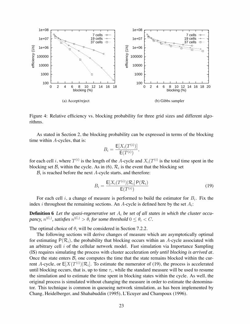
Figure 4: Relative ef"ciency vs. blocking probability for three grid sizes and different algo-rithms.
As stated in Section 2, the blocking probability can be expressed in terms of the blockingtime within A-cycles, that is:
Bi =E[Xi(T
(i))]
E(T (i)),
for each cell i, where T (i) is the length of the A-cycle and Xi(T(i) is the total time spent in the
blocking set Bi within the cycle. As in (6),Ri is the event that the blocking setBi is reached before the next A-cycle starts, and therefore:
Bi =E[Xi(T
(i))|Ri] P(Ri)
E(T (i))(19)
For each cell i, a change of measure is performed to build the estimator for Bi. Fix theindex i throughout the remaining sections. An A-cycle is de"ned here by the set Ai:
Definition 6 Let the quasi-regenerative setAi be set of all states in which the cluster occu-pancy,n(Ci), satisfiesn(Ci) > θi for some threshold0 ≤ θi < C.
The optimal choice of θi will be considered in Section 7.2.2.The following sections will derive changes of measure which are asymptotically optimal
for estimating P(Ri), the probability that blocking occurs within an A-cycle associated withan arbitrary cell i of the cellular network model. Fast simulation via Importance Sampling(IS) requires simulating the process with cluster acceleration only until blocking is arrived at.Once the state enters Bi one computes the time that the state remains blocked within the cur-rent A-cycle, or E[X(T (i))|Ri]. To estimate the numerator of (19), the process is accelerateduntil blocking occurs, that is, up to time τi, while the standard measure will be used to resumethe simulation and to estimate the time spent in blocking states within the cycle. As well, theoriginal process is simulated without changing the measure in order to estimate the denomina-tor. This technique is common in queueing network simulation, as has been implemented byChang, Heidelberger, and Shahabuddin (1995), L'Ecuyer and Champoux (1996).
23

Let X(t) be the occupancy process of the clusterCi of all the cliques where i belongs. Usethe aggregate arrival process at this cluster of surrounding cells, which is Poisson with intensityλ ≡
∑j∈Ci λj . The original process is modeled now using this arrival process to generate the
inter-arrival times Ak(i) ∼ exp(λ). Under this relabeling, Sk(i) is the epoch of the k-th localarrival at cluster Ci. Next, at arrival epochs Sk(i), the cell to which the arrival to the cluster isassigned is chosen to be cell j ∈ C with probability λj/λ. Holding times Hk(i) ∼ exp(µ) arei.i.d. exponential, as before. These quantities correspond to the actual holding times of the k-thcall to be connected within the cluster, regardless of the particular cell j ∈ Ci where it happensto belong. If the k-th arriving call to the cluster is blocked we setHk(i) = 0 by convention (thecall is not connected), rather than queueing the customer for future service. The process X(t)can be seen as a queueing model with parallel servers, but it behaves very differently from theGI/G/s/n model that was treated in Section3.4. The latter can be viewed as a truncation of aGI/G/s/∞ queue, while the former is a truncation of an infinite server queue.
In many queueing studies the discrete event model is used for simulation as well as forIS estimation. The discrete event simulation model for the process considers the generationof inter-arrival and holding times as needed, that is, Uk(i) = (Ak(i), Hk(i), Dk(i)) whereDk(i) ∈ Ci is the cell where the arrival occurs within the cluster. Let Uk(j) = (Ak(j), Hk(j))be the inter-arrival and holding times for cells j 6∈ Ci. The natural "ltration is given by:
FDEk = σ(U1(i), . . . , Uk(i)(i);U1(j), . . . , Uk(j)(j); j 6∈ Ci); k = 1, 2, . . . (20)
where exactly k(i) arrivals have occurred within the cluster Ci and k(j) arrivals at cell j 6∈ Ci atthe epoch of the k-th global arrival. The embedded occupancy process n(k) can be evaluatedfrom the information in FDEk and is therefore adapted to the "ltration (20), as required.
The usual problem for these systems is that the acceleration affects several holding timeseven after blocking has been detected and may slow down termination of the cycles. Sadowsky(1991) stops the change of measure for the service times from the arrival (τ−n) of the customerthat will be in service when customer τ
arrives "nding n in waiting. Although this is mathematically convenient, it turns out to beimpossible to simulate using the above DESmodel because τi is not measurable w.r.t. FDEk , k <τi: at the time of arrivals of the customers presently in the queue when τ "nds blocking,this fact is unknown. Devetsikiotis and Townsend (1993) propose to use another change ofmeasure from the moment that blocking occurs, in order to emptythe occupancy quickly forfast termination of theA-cycle. L'Ecuyer and Champoux (1996) seek to "nd a smaller stoppingtime in the hope of stopping the acceleration before blocking occurs. Instead we propose to doit using a different simulation model which in addition is
much simpler to code than the Discrete Event model.The simulation model is the Standard Clock technique of Vakili (1991), which corresponds
to the dynamical description of a multidimensional birth and death process. When the totaloccupancy of the current state is n, an exponential random variable with intensity Λn is usedto determine the inter-event time, or the time for the next event. Here
Λn =∑j
λj + nµ.
24

Next, the event typeis determined as a discrete random variable with distribution:
D =
aj : arrival at cell j w.p.
λjΛn
sj : termination of call at cell j w.p.njµ
Λn
where nj is the number of calls at cell j, so that n =∑
j nj .The appropriate "ltration for this process is
Fk = σ(T1, . . . , Tk;D1, . . . , Dk), k = 1, 2, . . . (21)
where Tk are the successive inter-event times and Dk the corresponding event types or deci-sions. The embedded occupancy process is updated by setting
nj(k + 1) =
nj(k) + 1 if n(k) 6∈ Bi and Dk+1 = aj ,nj(k)− 1 if Dk+1 = sj
n(Ci)k =
∑j∈Ci
nj(k), total cluster occupancy
Work has been done on applying importance sampling to other problems though uni-formization (Heidelberger, Shahabuddin, and Nicola, 1994), which creates events a a maximalrate Λ independent of the state, and then adjusts the probabilities by adding "ctitious, or nullevents. Use of the SC model for simulation may be more ef"cient because there is no needfor simulating null events. To emphasize that we apply Importance Sampling to the StandardClock simulation model, use the acronym ISSC.
Remark: Notice that, although the two models describe the same process (in distribution),the partial histories FDEk and Fk are not equivalent. Filtration (20) contains "ltration (21) butclearly, Hk is not measurable w.r.t. σ(T1, . . . , Tk; D1, . . . , Dk). If a particular change of mea-sure (such as rate-swapping) is BRE for the DES formulation, it does not necessarily mean thatit is also BRE for the SC formulation and vice versa, however for some models this may wellbe the case.
6 Static ISSC Estimation for Light Traffic
6.1 Change of Measure
In the light traf"c regime, assume that λi = kiε, i = 1, . . . K. Unlike the GI/G/s/∞ case,(11) need not hold for each channel on the trajectories where blocking occurs before the A-cycle ends and swapping rates as in (12) will not be optimal. Instead, consider the change ofmeasure that swaps aggregate arrival rates per cluster and inverse holding times.
Proposition 1 Consider the ISSC simulation model with initial state as the start of anA-cycle.Arrivals at the clusterCi have rateλ∗ = µ and holding times for the calls in the cluster have
25

rate µ∗ = λ. Other inter-arrival and holding times (outside the cluster) have the originalexponential distribution. Call the underlying measureP∗. Then:
P(Bi) = E∗
[e−(µ−λ)
∑τi−1
k=θ+1(n(Ci)(k)−1)Tk+1
(λ
µ
)k1−k2
1Ri
],
wherek1(j) is the total number of arrivals to cellj up to event numberτi (including blockedcalls), k1 =
∑j∈Ci k1(j) andk2 is the corresponding number of call completions (excluding
blocked calls).
Proof : Given the history of the process up to the k-th event (that is, given Fk) Tk+1 ∼exp(Λ∗n(k)), for n(k) = n1(k) + . . . + nK(k) the total occupancy of the process after eventk has occurred. The new event rate is a Fk-measurable random variable:
Λ∗n(k) = µ+∑j 6∈Ci
λj + λ∑j∈Ci
nj(k) + µ∑j 6∈Ci
nj(k),
and the event types now follow:
Dk+1 =
arrival at cell j ∈ Ci w.p.λiλ
µ
Λ∗n
arrival at cell j 6∈ Ci w.p.λjΛ∗n
termination of call at cell j ∈ Ci w.p.njλ
Λ∗ntermination of call at cell j 6∈ Ci w.p.
njµ
Λ∗n
.
Within an A-cycle, we perform this change of measure until the τi-th event occurs, whichis the "rst time that the state is in Bi. Because the
distributions of Tk+1 and Dk+1 are conditional on Fk, the change of measure de"nes amultiplicative martingale which is adapted to the "ltration Fk, k ≥ 1, and the correspondingRadon-Nikodym derivative is given by:
Lτi =
τi−1∏k=1
(Λn(k)
Λ∗n(k)
)e(Λ∗
n(k)−Λn(k))Tk+1 (22)
×τi−1∏k=1
(Λ∗n(k)
Λn(k)
)(∑j∈Ci
(λj
µ(λj/λ)
)1Dk+1=aj +
(µλ
)1Dk+1∈Si + 1Dk+1 6∈Si∩Ai
)
whereAi = aj : j ∈ Ci is the set of event types which are arrivals to the cluster and similarly,Si = sj : j ∈ Ci is the set of event types which are termination of calls within the cluster.From their de"nitions, it follows that:
Λ∗n − Λn = (µ− λ) + (λ− µ)∑j∈Ci
nj = −(µ− λ)(n(Ci) − 1)
where n(Ci) =∑
j∈Ci nj is the total occupancy of the cluster.
26

Simplifying the expression above,
Lτi = e−(µ−λ)∑τi−1
k=θ+1(n(Ci)(k)−1)Tk+1
[∏j∈Ci
(λ
µ
)k1(j)](µ
λ
)k2
= e−(µ−λ)∑τi−1
k=θ+1(n(Ci)(k)−1)Tk+1
(λ
µ
)k1−k2
, (23)
which proves the claim. /
Lemma 2 Whenλ < µ,Lτi1Ri < (λ/µ)C−θ,P∗ − w.p.1. (24)
In particular, Lτi1Ri < 1,P∗ − w.p.1., guaranteeing variance reduction of the ImportanceSampling estimator with the Standard Clock (ISSC).
Proof : Clearly λj < λ =∑
j∈Ci λj , and there are at least C on-going calls within the cluster atthe blocking time τi. At the time the A-cycle begins, there are (by De"nition 6) θ calls withinthe cluster. Thus acceleration begins when there are θ + 1 calls in the cluster. Because thestopping time within an A-cycle counts only the transitions from the start of the A-cycle upuntil blocking, on the set ω : τi < T (i) we have n(Ci)(k) ≥ θ + 1, k = 1, . . . , τi, whence
(µ− λ)
τi−1∑k=1
(n(Ci)(k)− 1)Tk+1 ≥ 0. (25)
Moreover, k1 =∑
j∈Ci k1(j) ≥ k2 + C − θ, giving the result. /
Theorem 2 The ISSC estimation that swaps the ratesλ andµ is BRE forP[Ri] as ε → 0,whenλi = kiε, for all cells i andθi = 0.
Proof : The proof is an application of Lemma 1. The upper bound is obtained with the resultof Lemma 2:
Lτi ≤(λ
µ
)C= d2ε
C , (26)
where d2 =∑
j∈Ci kj .It remains to show p(ε) ≥ d1ε
C . In order for blocking of cell i arrivals to occur, theoccupancy of one of the cliques in the cluster must necessarily attain level C. Let a minimalpath be a trajectory in which the "rst C events in an A-cycle which involve the acceleratedcluster are arrivals to the same clique. All minimal paths will cause blocking, and thus theirprobability is a lower bound for p(ε). The probability of such minimal paths is the probabilitythat each of the "rst C events be an arrival, and so:
p(ε) ≥(λiΛn
)C≥(kiε
Cµ
)C≥ d1ε
C , (27)
where λi is the smallest aggregate clique rate within cluster Ci and d1 = (ki/Cµ)C , with ki thesmallest of
∑s∈cj ks over the cliques cj ∈ Ci.
It follows by Lemma 1 that in this case, ISSC is BRE. /
Note that the condition θi = 0 is not a major limitation, since the modal cluster occupancywill be zero, and so θi = 0 gives the shortest A-cycles, which is desirable for simulations.
27

Acc
eler
ated
pro
cess
ing
Res
me
back
bone
fro
m s
ame
stat
e
Figure 5: Backbone and ribs simulation framework.
6.2 Numerical Results
An A-cycle must start with the state distribution being the equilibrium distribution conditionalon being on the boundary between A and A′. In the absence of importance sampling, this willalso be the distribution at
the end of the A-cycle. That means that multiple A-cycles can be simulated simply bysimulating the system for a long period, and marking off the A-cycles. However, importancesampling disturbs the distribution, and the distribution of the state at the end of an A-cyclecannot be used as the starting state for the next A-cycle. Instead of this, when the start ofan A-cycle is detected, the simulation will be suspended, and a second simulation will bestarted from the current state n. This second simulation will be accelerated until blockingoccurs (or the current A-cycle ends) and the original measure is used to determine the timespent in blocking states until the end of the current A-cycle. The original simulation is thenrecommenced from state n, until the start of the next A-cycle. This gives rise to the backboneand ribs arrangement, seen in Figure 5. A second advantage of this approach is that the lengthof an A cycle, as required by (4), may be estimated more accurately (with lower variance) fromthe unaccelerated A-cycles.
Each A-cycle only estimates the blocking probability in a single cell. Thus in order toestimate the blocking probability in each cell, it is necessary to run separate simulations foreach cell. Fortunately, it is not necessary to simulate the backbone separately. Instead,separate ribs can be started each time the backbone starts an Ai-cycle for any cell i. Notethat a single event may be the start of Ai-cycles for more than one i, and each of these must beconsidered.
The ribs may be further simpli"ed by noting that the set A′i contains no blocking statesfor cell i. Thus, once an accelerated Ai-cycle has left the set Ai, the entire time spent inblocking states will already have occurred. This means that the rest of the Ai-cycle need notbe simulated, even though a considerable amount of time may be spent in the set A′i before theAi cycle is truly over.
The ISSC with θi = 0 for ρ → 0 was tested on three sizes of network: 4, 7 and 37 cells.Figure 6 compares these results with those of the "ltered Gibbs sample of Section 4.2. Theresults clearly show that the relative error of the estimated network blocking probability is
28

10
100
1000
10000
0.0001 0.001 0.01 0.1 1 10
rela
tive
effic
ienc
y
load (Erlangs / cell)
4 cells, IS7 cells, IS
37 cells, IS4 cells, FGS7 cells, FGS
37 cells, FGS
(a) ef"ciency against load
0.001
0.01
0.1
1e-06 1e-05 0.0001 0.001 0.01 0.1 1
rela
tive
stan
dard
dev
iatio
n (1
e5 s
ampl
es)
blocking probability
4 cells, IS7 cells, IS
37 cells, IS4 cells, FGS7 cells, FGS
37 cells, FGS
(b) error against blocking
Figure 6: Relative ef"ciency and relative error for importance sampling (IS) and "ltered Gibbssampler (FGS) for light loads
bounded as ρ→ 0.
7 Dynamic ISSC Estimation for High Capacity
7.1 Change of Measure
It is unlikely that future networks will be operated at extremely low utilisation, as was assumedin the previous section. Engineers are more interested in the behaviour as the capacity in-creases. This is particularly true of wavelength continuous WDM trunk networks, which aremathematically analogous to the cellular networks described so far (see Andrew and Vazquez-Abad, 2001). It is possible to overcome the restriction that λ < µ in the previous section byallowing the arrival and service rates to be state dependent.
This section addresses the simulation of the important regimes of C →∞ with ρ constant,and C → ∞ with ρ/C constant, both of which cause blocking to become a rare event. Swap-ping λ and µ as in the previous section will not yield BRE for high capacity regimes (evenwhen λ < µ) because as C → ∞ the lower bound on P[Ri] goes to zero, and blocking doesnot become more likely under the star measure P∗. A change of measure which is optimal inthe case of a C parallel server system with no waiting will be presented, and applied to thecellular case. It is suboptimal in this latter context, but it provides a dramatic improvementover simulation using the original measure.
Consider again the Standard Clock simulation model and let the change of measure be suchthat the total event rate is the same as for the original measure: Λ∗(n) = Λ(n), when the state isn. When an event occurs, it is a departure (or an arrival) to cell j 6∈ Ci with probability λj/Λn
(equivalently, njµ/Λn) just as for the original measure. Arrivals (departures) to the cluster willnow occur with probability λ∗(n)/Λn (or µ∗(n)/Λn, respectively). The proportion of arrivalsto the cluster that go to cell j ∈ Ci remains "xed at λj/λ. Under this change of measure, therates are no longer constant, but depend on the state, hence the name dynamic ISSC.
29

It is straightforward to calculate now the Radon-Nikodym derivative:
Lτi =
τi−1∏k=1
(∑j∈Ci
(λ
λ∗(n(k))
)1Dk+1=aj +
(µ
µ∗(n(k))
)1Dk+1∈Si + 1Dk+1 6∈Si∩Ai
),
independent of the inter-arrival times.Speci"cally, if n = n(Ci)(k) is the clusteroccupancy of the process at event k, let the rates
be de"ned by the recurrence relation:
µ∗(n) =λµ
λ∗(n− 1)(28a)
λ∗(n) = λ+ n(µ− µ∗(n)). (28b)
Notice that the rates under the star measure (28) only depend on the cluster occupancy,rather than the whole state of the process n(k). This is related to swapping the arrival andservice rates of (12) in the following sense.
Lemma 3 Under the update rule (28), for any initial0 < µ∗(1) < µ,
limn→∞
λ∗(n)/n = µ (29a)
limn→∞
µ∗(n)n = λ. (29b)
Proof : We will "rst show that µ∗(n) → 0 as n → ∞. By induction, 0 < µ∗(n) < µ for alln ≥ 1, and hence µ∗(n) has a convergent subsequence. To see that µ is not an accumulationpoint, note that this would imply µ∗(n) = µ − φ(n) for some φ(n) = o(1), φ(n) 6≡ 0. Thenby (28a), λ∗(n)− λ ∼ φ(n), but by (28b), λ∗(n)− λ ∼ nφ(n), which is a contradiction. Thusthere is a strictly increasing sequence n(m) ∈ N and a µ∗ ∈ [0, µ) such that µ∗(n(m)) → µ∗
asm→∞. Thus there is a δ = µ− µ∗ > 0 such that
λ∗(n(m+ 1))− λ∗(n(m)) = (n(m+ 1)− n(m))(µ− µ∗) + o(1) > δ + o(1).
Thus λ∗(n(m)) → ∞, and by (28a), µ∗(n(m)) → µ∗ = 0. Since the sequence m(i) wasarbitrary, 0 is the unique accumulation point, and µ∗(n)→ 0 as n→∞.
By (28b) and the convergence of µ∗(n),
λ∗(n+ 1)− λ∗(n) = µ+ o(1).
Thus λ∗(n) = λ∗(1) +∑n
k=2(µ+o(1)) = nµ+o(n), and λ∗(n)/n→ µ as n→∞. The resultthen follows from (28a). /
This asymptotic form is analogous to the static change of measure for an M/M/n/∞queue. AnM/M/s/∞ queue has a maximum of s servers active in the limit, and so the changeof measure is static in that case. The change of measure of (28) is dynamic, re#ecting the factthat the number of active servers increases continually as the size of the system increases.
Theorem 3 Consider a birth and death process with ratesλ(n) ≡ λ, µ(n) = nµ onθ, . . . , C.Let τ be the first hitting time ofC, T the first return to stateθ andR = τ < T. Then theISSC estimator forP(R) using the dynamic rates in (28) starting withµ∗(θ+ 1) = 0 is asymp-totically optimal in the limit ofC → ∞. Moreover, it is exactly optimal: the variance of theestimate is zero even for finiteC.
30

Proof : With µ∗(θ + 1) = 0, P∗(R) = 1 since the A-cycle is not allowed to end until blockingoccurs. This violates the absolute continuity condition that for every x ∈ S, P(x) > 0 ⇒P∗(x) > 0. However, as mentioned in Section 6, PcRi << P∗. This follows because onthe event Ri, blocking occurs before the A-cycle is over, thus no trajectory on Ri can havea transition from θ + 1 back to θ (this would start a new A-cycle). Thus for every x ∈ Ri,P(x) > 0⇒ P∗(x) > 0, and the change of measure is valid for the estimation of P(Ri).
On any path leading to the blocking boundary C, any transition due to a call terminationfrom state n to n−1must necessarily be followed in some future stage by a matching transitionfrom n−1 to n: otherwise it is impossible to achieve full occupancy. The corresponding factorscontributing to Lτ are then:(
µ(n)
µ∗(n)
)(λ(n− 1)
λ∗(n− 1)
)=
(λ(n− 1)
λ
)(λ
λ∗(n− 1)
)= 1,
therefore all such loops cancel out their contributions. The only remaining contributions to Lτare the factors for the minimal blocking path θ + 1 → θ + 2 → θ + 3 → . . . → C, whichyields:
Lτ =C−1∏k=θ+1
λ
λ+ k(µ− µ∗(k)), (30)
which is a deterministic function of C, thus optimal. /
Note that for a "xed µ∗(θ+ 1), the rates are independent of C. The optimal adaptivity to Ccomes from the fact that the rates change as the actual current occupancy changes.
In the cellular network case, we identify the birth and death process as the cluster occu-pancy process: while it remains true that to achieve blocking at a state nτ ∈ Bi all backwardtransitions from n to n − 1 will cancel out from forward transitions from n − 1 to n, now theISSC estimator is:
Lτi =
n(Ci)τ −1∏k=θ
λ
λ+ k(µ− µ∗(k)),
and the "nal cluster occupancy n(Ci)τ satis"es C ≤ n
(Ci)τ ≤ mC, where m is the number
of cliques in the given cluster, which depends on the interconnectivity of the network. Thevariance of Lτi is thus dependent on the variation of the distribution of the cluster occupancyat blocking.
7.2 Implementation considerations
7.2.1 Subsampling the ribs
The correlation between consecutive A-cycles in the backbone can be very signi"cant. Inorder to reduce this, it is possible to subsample the A-cycles, and only start a rib for everykth A-cycle. This greatly increases the amount of work required to simulate the backbone.However, an A-cycle which is blocked may be very much longer than a typical A-cycle,especially when the load is a small fraction of the number of channels, and so the backboneis often a small proportion of the simulation time. Moreover, the backbone is shared betweenmany cells, making subsampling very worth while. Estimating the variance of a ratio can be
31

performed following Bratley, Fox, and Schrage (1987), when both numerator and denominatorare sample averages of Markov processes with exponentially decaying covariances, instead ofiid random variables. In this case, if Bi = E[Y ]/E[T ], then the random variable obtainedduring the l-th A-cycle:
Zl = kYl1lmodk=0 −Bi Tl
has zero expectation. Here Yi represents the estimate of the numerator obtained from the l-thrib (of which only one out of k is used) and Tl is the estimate of the cycle length (which wecalled T (i) before). Then the estimator obtained with S consecutive A-cycles satis"es:
Var[Bi(S)] = Var
(kS
∑Sl=1 Yl1lmodk=0
1S
∑Sl=1 Tl
)≈ K1 Var
(1
S
S∑l=1
Zl
),
whereK1 is a constant depending on E[T ]2, but independent of the sample size S. The optimalvalue of k can be obtained by noting that
Var
(1
S
S∑l=1
Zl
)≈ KY (k/S) +KT/S,
where KY depends on Var[Y ] and KT depends on B2i Var[T ]. The covariance term decreases
as S2. On the other hand,CPU[Bi(S)] = lT (k/S) + lY S,
where lT and lY are the mean lengths of unaccelerated and accelerated A-cycles respectively.The ef"ciency (5) is then maximised by setting
k∗ ≈√KY lYKT lT
. (31)
These values can be estimated coarsely from a short pilot simulation, which can also serve asthe warm-up to achieve steady state. When acceleration
is used, k∗ is of the order of 10, to within one order of magnitude. Without acceleration, k∗
is actually often less than 1, indicating that there may be value in running multiple ribs fromthe same point in the backbone.
7.2.2 Choice of quasi-regenerative cycles
When the load, λ/µ, is not negligible, the probability that the cluster will be completely emptyis small. Thus if θ is too small, like θ = 0 as is used for single server queues, then the A-cyclesbecome unmanageably long. This has several implications. The most obvious result is that thesimulation time increases in proportion. The seriousness of this is to some extent alleviatedby the fact that longer A-cycles produce better estimates of the proportion of time spent inblocking states within an A-cycle.
The more serious problem with long A-cycles is that the blocking states become a smallproportion of the A-cycles, even given that blocking occurs. The assumption behind the ISscheme proposed here is that A-cycles in which blocking occurs are rare events, but if blockingdoes occur, it does so for a signi"cant proportion of theA-cycle. Thus the system is accelerateduntil the point when blocking "rst occurs, and is then allowed to relax back to "nish itsA-cycle.
32

If λ and C are both large, then empty clusters become rarer than blocking, and most A-cyclescontain a period of blocking, reducing the effectiveness of the acceleration.
The length of A-cycles is minimised by maximising the rate of crossing the boundary be-tween sets A and A′ of the embedded Markov Chain. Since the stationary rate at which theprocess crosses from any state with n(Ci) = θ to n(Ci) = θi + 1 equals the stationary rate atwhich it crosses from n(Ci) = θi + 1 to n(Ci) = θ. This rate is state dependent:
λπ(θi)
Λn
, n ∈ S(θi)
where S(θi) is the subset of the state space S that has n(Ci) = θ channels busy in cluster Ci.Naturally, one seeks a unique value θi that maximises this rate, such as a maxmin optimiser. Asimple observation however simpli"es this task: for many systems with several cells, for theregime where both C and λ grow, the value of Λn will be nearly constant, and the value thatmaximises the numerator is the mode of the stationary distribution π(·), or θi ≈
∑j∈Ci λj/µ
(assuming that blocking does not signi"cantly distort the state distribution, and that the meanand mode of π are very close).
Next, in order to guarantee that Lτi < 1 when blocking occurs, it was required that θi ≤ C,since Lτi can exceed 1 whenever the number of departures exceeds the number of arrivalsduring the acceleration period. Thus we use the value
θi = max
(∑j∈Ci
λj/µ, C
). (32)
It is possible that in some instances the overall variance can be reduced by using θi > C,since the probability of a greater number of departures than arrivals leading to blocking maybe small. This is the subject of ongoing research. There may also be bene"t in using values ofθi larger than
∑j∈Ci λj/µ
(but less thanC). AlthoughA cycles become longer, the time spent in the setA′ (n(Ci) < θi)need not be simulated in the ribs, since blocking cannot occur in this case. It must still besimulated in the backbone to estimate the mean duration of an A-cycle, but this is sharedbetween all cells.
7.3 Simulation results
The dynamic change of measure was shown to be a.o. for the probability of blocking occurringwithin an A-cycle, P(Ri), in the case of a single cell. Figure 7 shows the relative ef"ciency forthe true probability of blocking in this case. As C increases, the proportion of each time spentin a blocking state decays, even on those A-cycles which contain blocking. This accounts forthe slight reduction in ef"ciency as the blocking rate decreases. However, this reduction is verymuch smaller than occurs without acceleration.
Figure 8 shows the relative ef"ciency of the accelerated and non-accelerated methods fora seven-cell cellular system, for a range of loads and a range of capacities (normalised bythe load). The ISSC subsamples the A-cycles in the backbone by a factor of k = 10. Thesimulations without acceleration use k = 1, as the rib A-cycles are shorter and the variance ofthe corresponding estimator is higher. These results do not suggest that ISSC is a.o. for network
33

0.1
1
10
100
1000
10000
100000
0 5 10 15 20 25
rela
tive
effic
ienc
y
C / ρ
accnon-accρ = 0.5
ρ = 1ρ = 2ρ = 4ρ = 8
(a) ef"ciency against load
0.1
1
10
100
1000
10000
100000
1e-35 1e-30 1e-25 1e-20 1e-15 1e-10 1e-05 1
rela
tive
effic
ienc
y
pr(blk)
accnon-accρ = 0.5
ρ = 1ρ = 2ρ = 4ρ = 8
(b) ef"ciency against blocking
Figure 7: Relative ef"ciency for importance sampling (ISSC), A-cycle framework without IS,and the simple simulation, all in a single cell.
blocking as C → ∞. However, IS substantially reduces the rate at which the performancedegrades for large C.
The reason for the reduced ef"ciency is that the acceleration is applied to all cells in acluster. For a constant load, as C increases the (true)
expected cluster occupancy on blocking satis"es E[n(Ci)|Bi]/C → 1, since arrivals at eachcell are independent, and only one clique need be full. However, because the accelerationis applied to all cells in the cluster, the cells outside the clique which caused blocking arealso "lled up. Thus the expected cluster occupancy at blocking under the new measure issigni"cantly larger than under the original measure. That is, outcomes with a high clusteroccupancy are accelerated too much, increasing the variance.
It seems from Figure 8(a) that the improvement decreases as the load increases. However,this is largely due to the fact that the rate at which the blocking decreases for increasing C isdifferent. Figure 8(b) shows the relative ef"ciency against the blocking probability. This showsthat the change in slope of the curves is similar over a range of loads. Note that in the rangewhich is of most interest to engineers, with blocking between 10−6 and 10−2, the accelerationconsistently outperforms the non-accelerated simulation.
Figure 8(b) also includes results for a simple estimation scheme, which does not sim-ulate A-cycles and use (4), but instead simulates only the backbone and simply counts theproportions of calls which are blocked. This shows a constant factor improvement over thenon-accelerated A-cycles, which is largely due to its ability to estimate blocking over the en-tire network at once, rather than focusing on a single cell in each A-cycle.
The key advantage of ISSC over the "ltered Gibbs sampler is that it can be used even whenthe stationary distribution does not have a product form, or the closed form is not know. Thisis the case when existing calls cannot be rearranged. Figure 9 shows the performance of ISSCfor a seven cell network when existing calls are not rearranged.
34
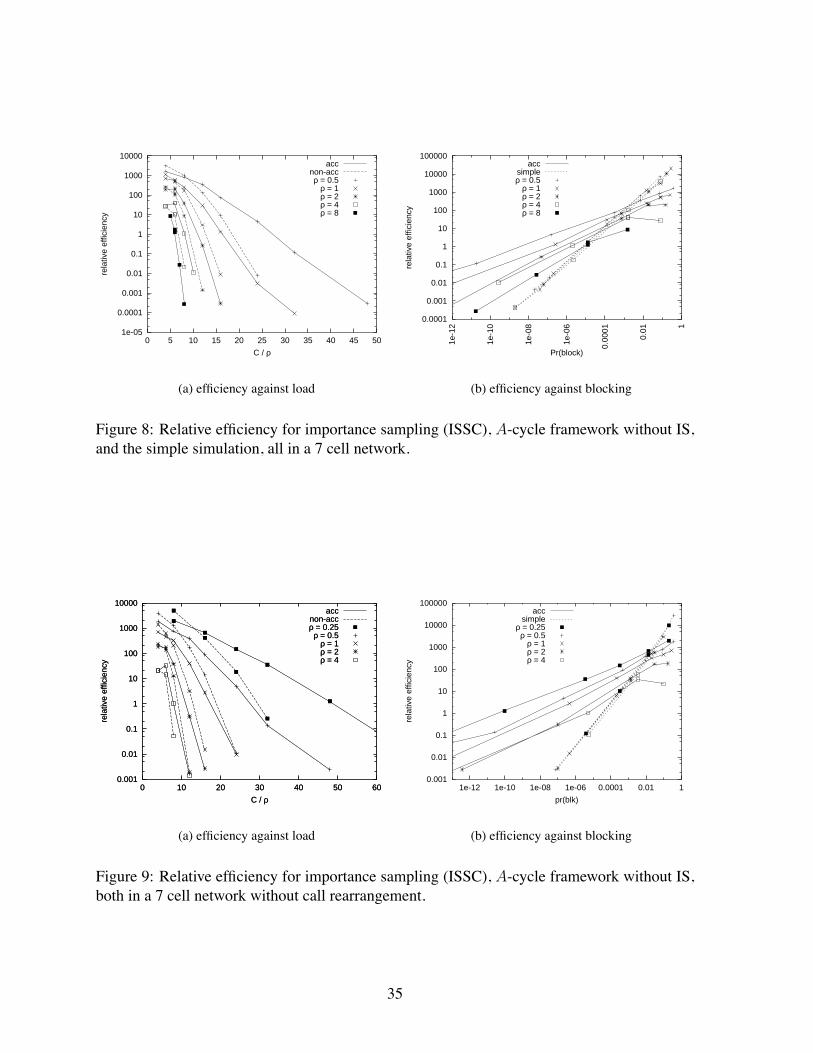
1e-05
0.0001
0.001
0.01
0.1
1
10
100
1000
10000
0 5 10 15 20 25 30 35 40 45 50
rela
tive
effic
ienc
y
C / ρ
accnon-accρ = 0.5
ρ = 1ρ = 2ρ = 4ρ = 8
(a) ef"ciency against load
0.0001
0.001
0.01
0.1
1
10
100
1000
10000
100000
1e-1
2
1e-1
0
1e-0
8
1e-0
6
0.00
01
0.01 1
rela
tive
effic
ienc
y
Pr(block)
accsimpleρ = 0.5
ρ = 1ρ = 2ρ = 4ρ = 8
(b) ef"ciency against blocking
Figure 8: Relative ef"ciency for importance sampling (ISSC), A-cycle framework without IS,and the simple simulation, all in a 7 cell network.
0.001
0.01
0.1
1
10
100
1000
10000
0 10 20 30 40 50 60
rela
tive
effic
ienc
y
C / ρ
accnon-accρ = 0.25
ρ = 0.5ρ = 1ρ = 2ρ = 4
0.001
0.01
0.1
1
10
100
1000
10000
0 10 20 30 40 50 60
rela
tive
effic
ienc
y
C / ρ
accnon-accρ = 0.25
ρ = 0.5ρ = 1ρ = 2ρ = 4
(a) ef"ciency against load
0.001
0.01
0.1
1
10
100
1000
10000
100000
1e-12 1e-10 1e-08 1e-06 0.0001 0.01 1
rela
tive
effic
ienc
y
pr(blk)
accsimple
ρ = 0.25ρ = 0.5
ρ = 1ρ = 2ρ = 4
(b) ef"ciency against blocking
Figure 9: Relative ef"ciency for importance sampling (ISSC), A-cycle framework without IS,both in a 7 cell network without call rearrangement.
35

8 Concluding Remarks
This paper has addressed two aspects of rare events in the calculation of network blockingprobabilities. The "rst, the rarity of feasible states in acceptance/rejection Monte Carlo tech-niques, is merely an artifact of a common technique. This is removed by using a MCMCmethod, namely the Gibbs sampler. The Gibbs sampler clearly outperform the usual accep-tance/rejection method and its relative ef"ciencies grow with problem size and with increasingload.
The second class of rare events is intrinsic to the problem. It is that blocking is a rare eventwhen the load is relatively low. To overcome this problem, we implemented the main ideasof fast simulation using standard queueing-like results under the discrete event framework forsimulation. Next we suggest using this change of measure for the standard clock frameworkfor simulation, which entails signi"cantly less computational effort.
When dealing with cellular network lay-outs, it may be that some regions of the spacesatisfy the conditions for which the MCMC methods are best suited, while other regions mayfall under the rare event framework. We believe that hybrid methods may well prove to be themost ef"cient ones in practice.
References:
Alexopoulos, C., and A. Seila. 1998. Output data analysis. chapter 7. In Handbook ofSimulation, ed. J. Banks, 225272. John Wiley & Sons.
Andrew, L., and F. Vazquez-Abad. 2001. Fast simulation of wavelength-continuous WDMnetworks. (In preparation).
Asmussen, S., and H. Nielsen. 1995. Ruin probabilities via local adjustment coef"cients. J.Appl. Probab., 32:736755.
Boucherie, R. J., andM.Mandjes. 1998. Estimation of performance measures for product formcellular mobile communications networks. Telecommunication Systems, 10:321354.
Bratley, P., B. Fox., and L. Schrage. 1987. A Guide to Simulation. Second ed. New York:Springer-Verlag.
Breiman, L. 1992. Probability. Classics in Applied Mathematics, SIAM.Bremaud, P. 1999. Markov Chains, Gibbs Fields, Monte Carlo Simulation, and Queues. Texts
in Applied Mathematics, 31, New York: Springer.Bucklew, J. A. 1990. Large Deviations Techniques in Decision Simulation and Estimation.
New York: Wiley.Chang, C.-S., P. Heidelberger., and P. Shahabuddin. 1995. Fast simulation of packet loss rates
in a shared buffer communications switch. ACM Trans. Model. Comput. Simul., 5(4):306325.
Choudhury, G. L., K. K. Leung., and W. Whitt. 1995. An algorithm to compute block-ing probabilities in multi-rate multi-class multi-resource loss models. Adv. Appl. Prob.,27:11041143.
Cox, D., and D. Reudink. 1972. Dynamic channel assignment scheme in large cellular-structured mobile communication systems. IEEE Trans. Commun., COM-26:432438.
Cox, D., and D. Reudink. 1973. Increasing channel occupancy in large scale mobile radiosystems: dynamic channel reassignment. IEEE Trans. Vehic. Technol., VT-22:218222.
Devetsikiotis, M., and K. Townsend. 1993. Statistical optimization of dynamic importancesampling parameters in ef"cient simulation of communication networks. IEEE/ACM Trans.
36

Networking, 1(3):293305.Dziong, Z., and J. W. Roberts. 1987. Congestion probabilities in a circuit-switched integrated
services network. Perf. Eval., 7:267284.Everitt, D., and N. Macfadyen. 1983. Analysis of multicellular mobile radiotelephone systems
with loss. Br. Telecom Technol. J., 1(2):3745.Gaivoronski, A., and E.Messina. 1996. Optimization of stationary behavior of general stochas-
tic discrete event dynamic systems. In Proceedings of WODES ’96. IEE Editors.Gilks, W., S. Richardson., and D. Spiegelhalter. 1996. Markov Chain Monte Carlo in Practice.
London: Chapman and Hall.Glynn, P., andW.Whitt. 1992. The asymptotic ef"ciency of simulation estimators. Operations
Research, 40(3):505520.Harvey, C., and C. Hills. 1979. Determining grades of service in a network. In 9th Interna-
tional Teletraffic Congress ITC9, paper 626.Heidelberger, P., P. Shahabuddin., and V. Nicola. 1994. Bounded relative error in estimating
transient measures of highly dependable non-Markovian systems. ACM Trans. Model.Comput. Simul., 4(2):137164.
Kelly, F. P. 1979. Reversibility and Stochastic Networks. New York: Wiley.Kelly, F. P. 1991. Loss networks. The Annals of Probability, 1:319378.Larson, H. J. 1973. Introduction to the Theory of Statistics. New York: John Wiley & Sons.Lassila, P., and J. Virtamo. 2000. Nearly optimal importance sampling for Monte Carlo simu-
lation of loss systems. COST report COST257TD(00), Helsinki University of Technology.Lassila, P. E., and J. T. Virtamo. 1998a. Ef"cient Monte Carlo simulation of product form
systems. In Proc. Nordic Teletraffic Seminar (NTS) 14, Copenhagen Denmark.Lassila, P. E., and J. T. Virtamo. 1998b. Variance reduction in Monte Carlo simulation of
product form systems. Electronics Letters, 34(12):12041205.L'Ecuyer, P., and Y. Champoux. 1996. Importance sampling for large ATM-type queueing
networks. In Proceedings of the 1996 Winter Simulation Conference, 309316. IEEEPress.
Lee, W. 1995. Mobile Cellular Telecommunications. 2nd ed. McGraw Hill.Mandjes, M. 1997. Fast simulation of blocking probabilities in loss networks. European
Journal of operations Research, 101:393405.Mitra, D., and J. A. Morrison. 1994. Erlang capacity and uniform approximations for shared
unbuffered resources. In Proc. 14th Int. Teletraffic Congress, 875886, Amsterdam. Else-vier.
Mouly, M., and M.-B. Pautet. 1992. The GSM System for Mobile Communications. TelecomPublishing. ISBN 2-9507190-0-7.
Nelson, R. 1993. The mathematics of product form queuing networks. Computing Surveys,25(3):339369.
Neuts, M. F. 1981. Matrix-Geometric Solutions in Stochastic Models: An Algorithmic Ap-proach. Baltimore, MD: Johns Hopkins University Press.
Pallant, D. L., and P. G. Taylor. 1995. Modeling handovers in cellular mobile networks withdynamic channel allocation. Operations Research, 43(1):3342.
Pinsky, E., and A. E. Conway. 1992. Computational algorithms for blocking probabilities incircuit-switched networks. Ann. Operat. Res., 35:3141.
Raymond, P.-A. 1991. Performance analysis of cellular networks. IEEE Trans. Commun.,39(12):17871793.
37

Redl, S., M. Weber., and M. Oliphant. 1995. An Introduction to GSM. Artech House.Reiser, M., and S. Lavenberg. 1980. Mean-value analysis of closed multichain queuing net-
works. J. ACM, 27(2):313322.Ross, K., and J. Wang. 1992. Monte-Carlo summation applied to product-form loss networks.
Probability in the Engineering and Information Sciences, 6:323348.Ross, K. W., D. H. K. Tsang., and J. Wang. 1994. Monte Carlo summation and integration
applied to multiclass queuing networks. J. ACM, 41(6):11101135.Ross, S. 1993. Introduction to Probability Models. Fifth ed. Boston: Academic Press.Ross, S. 1997. Simulation. Second ed. Boston: Academic Press.Sadowsky, J. S. 1991. Large deviations theory and ef"cient simulation of excessive backlogs
in a GI/GI/m queue. IEEE Trans. Autom. Control, 36(12):13831394.Vakili, P. 1991. Using a standard clock technique for ef"cient simulation. Operations Research
Letters, 10:445452.Vazquez-Abad, F., and L. Andrew. May, 2000. Filtered Gibbs sampler for estimating blocking
probabilities in WDM optical networks. In Proc. 14th European Simulation Multiconfer-ence, ed. D. Landeghem, 548ff, Ghent, Belgium. Society for Comuter Simulation.
Vazquez-Abad, F., and P. LeQuoc. 2001. Sensitivity analysis for ruin probabilities. Journal ofthe Operational Research Society, 52(1):7181.
Yates, J. 1997. Performance analysis of dynamically-recon"gurable wavelength division mul-tiplexed networks. PhD thesis, University of Melbourne, Australia.
Zahorjan, J., D. Eager., and H. Sweillam. 1988. Accuracy, speed and convergence of approxi-mate mean value analysis. Perf. Eval., 8:255270.
A Estimating Variance
Whenever each sample Ys is unbiased, their mean Y (S) will also be unbiased. However, thevariance of Y (S) may be dif"cult to estimate when the samples are highly correlated. Weare interested in estimating blocking probabilities. The general simulation framework usedis to simulate some underlying process Xk, k = 1, 2, . . ., such as a Markov Chain MonteCarlo (MCMC) process or the birth and death process of Section 2. Then it is possible toset Ys ∈ 0, 1 to be an indicator of Xs being a blocking state. Some underlying processesintroduce considerable correlation, so that from a point when Ys = 0, it may take a long time tbefore an observation yields a non-zero value for Ys+t. In order to calculate a variance of Y (S)in the presence of correlation, the batch means method reviewed in Alexopoulos and Seila(1998) can be used. It is based on regrouping β consecutive samples to form a batch meanYs, s = 1, . . . , S and simulating a total of S batches. The idea is that if β is large enough, thenconsecutive batch means will be approximately independent and the CLT is applied to thesequantities. An extensive study on the choice of β, S for accurate estimation of the con"denceinterval is provided in Alexopoulos and Seila (1998) and suggests that choosing β ≈ S may beoptimal.
To alleviate the problem of high correlations of consecutive values,periodic sampling of the sequence Ys could in principle be used to reduce the variance
of the estimation. Let t denote the sampling period. Then if Ys, s = 1, 2, . . . are unbiased,
38

the average of the observations Ykt, k = 1, 2, . . . is also unbiased, yielding the estimator:
Ys =1
β
β∑k=1
Ysβt+kt (33)
Y (S) =1
S
S∑s=1
Ys (34)
V (S) =1
S − 1
S∑s=1
(Ys − Y (S))2,
where V (S) is the estimated variance of a single batch mean, Ys, derived from S batches.For S ≥ 10 the normal approximation gives the approximate con"dence interval:
CI : Y (S)± z1−α/2
√V (S)
S. (35)
As t grows, it may suf"ce to consider smaller values of β, as the samples themselves becomeless correlated.
39