simulation for locating marine...

SIMULATION FOR LOCATING MARINE OUTFALLS

DR. R MANIVANAN Assistant Research Officer

Central Water And Power Research Station, Pune-24

1. INTRODUCTION

In coastal areas seawater provides an inexhaustible source of cooling water and also a sink for disposal of heated water from power station. For optimizing the efficiency of power generation, it is essential to locate the intake/outfall to minimize the recirculation of warm water discharge under the prevailing environmental site conditions. Desalination plants are also being widely used in coastal areas for providing freshwater to overcome the water shortage. Here also it is essential to locate the intake/outfall to minimize the recirculation of brine water discharge under the prevailing environmental site conditions. Two typical mathematical model studies are described here. One is regarding warm water dispersion and the other is regarding brine water dispersion. 2. MODELLING TECHNIQUE For these studies, numerical models MIKE21-HD (DHI, 2004) and MIKE21-AD (DHI, 2004) were used for simulation of coastal hydrodynamics and dispersion of warm/brine water in coastal waters respectively. These mathematical models are developed for two-dimensional free surface flows by Danish Hydraulics Institute (DHI), Denmark and are widely used commercial software. Brief descriptions of these models are given below. 2.1 The Hydrodynamic Model

The hydrodynamic model MIKE21-HD was used for simulation of water levels and flows in coastal areas. It simulates unsteady two-dimensional flows in coastal area and is based on the following non-linear vertically integrated 2-D equations of conservation of mass and momentum.

[ ]

)2(0)(

)()(122

222

=+−Ω−

+−+

++

+

+

xaw

y

yxyxxxw

xyx

t

phfVVQ

hhhC

QPgPghS

hPQ

hPP

ρ

ττρ

)1(0=++ yxt QPS[ ]

)3(0)(

)()(122

222

=+−Ω−

+−+

++

+

+

yaw

x

xxyyyyw

yxy

t

phfVVP

hhhC

QPgQghS

hPQ

hQQ

ρ

ττρ

Training Course on Coastal Engineering & Coastal Zone Management

“Simulation for Locating Marine Outfalls” by Dr. R Manivanan, ARO, CWPRS 2

2

where S=surface elevation (m), P, Q = flux densities in x, y directions (m2/s), h=water depth (m), C=Chezy resistance (m1/2/s), V, Vx, Vy = wind speed and components in x, y directions (m/s), f=wind friction factor, Ω= Coriolis parameter, pa=atmospheric pressure, τxx, τyy, τxy=components of effective shear stress(kg/m2), x,y = space coordinates (m), t= time (s). These equations are numerically solved by Alternate Direction Implicit (ADI) finite difference technique leading to formation of tri-diagonal matrices, which can be solved efficiently. 2.2 The thermal/salinity dispersion model The numerical model MIKE21-AD simulates dispersion of warm/saline water in coastal waters. It is based on the following non-linear vertically integrated 2-D equation of conservation of heat/salinity which takes into account advection, dispersion, warm/saline water source and sink.

(hC)t +(uhC)x +(vhC)y = (h Dx Cx )x + (h Dy Cy )y + S (5)

where, T = rise in temperature (deg. C), u,v =horizontal velocity components in x, y directions (m/s), Dx , Dy =dispersion coefficients in x, y directions (m2/s), S = source/sink discharge ( m3/s/m2). F = heat decay coefficient(s-1). C = rise in salinity (ppt). These equations are numerically solved by an explicit finite difference scheme. As it is well known, 2D models are depth averaged. Therefore the variation of parameters over the vertical is not simulated. It is to be noted that model simulates the far field advection-dispersion of the warm/saline water. It does not simulate the near field consisting of strong mixing near the point of outfall. 3. SIMULATION OF WARM WATER DISPERSION Kalpakkam is located on the east coast of India, about 70 km south of Chennai in TamilNadu State. Madras Atomic Power Station (MAPS) having two units of 220 MW was established at Kalpakkam in 1983-85. MAPS is operating on once-through cooling

)4()()()()()( SThFThDThDvhTuhThT yyyxxxyxt +−+=++



3

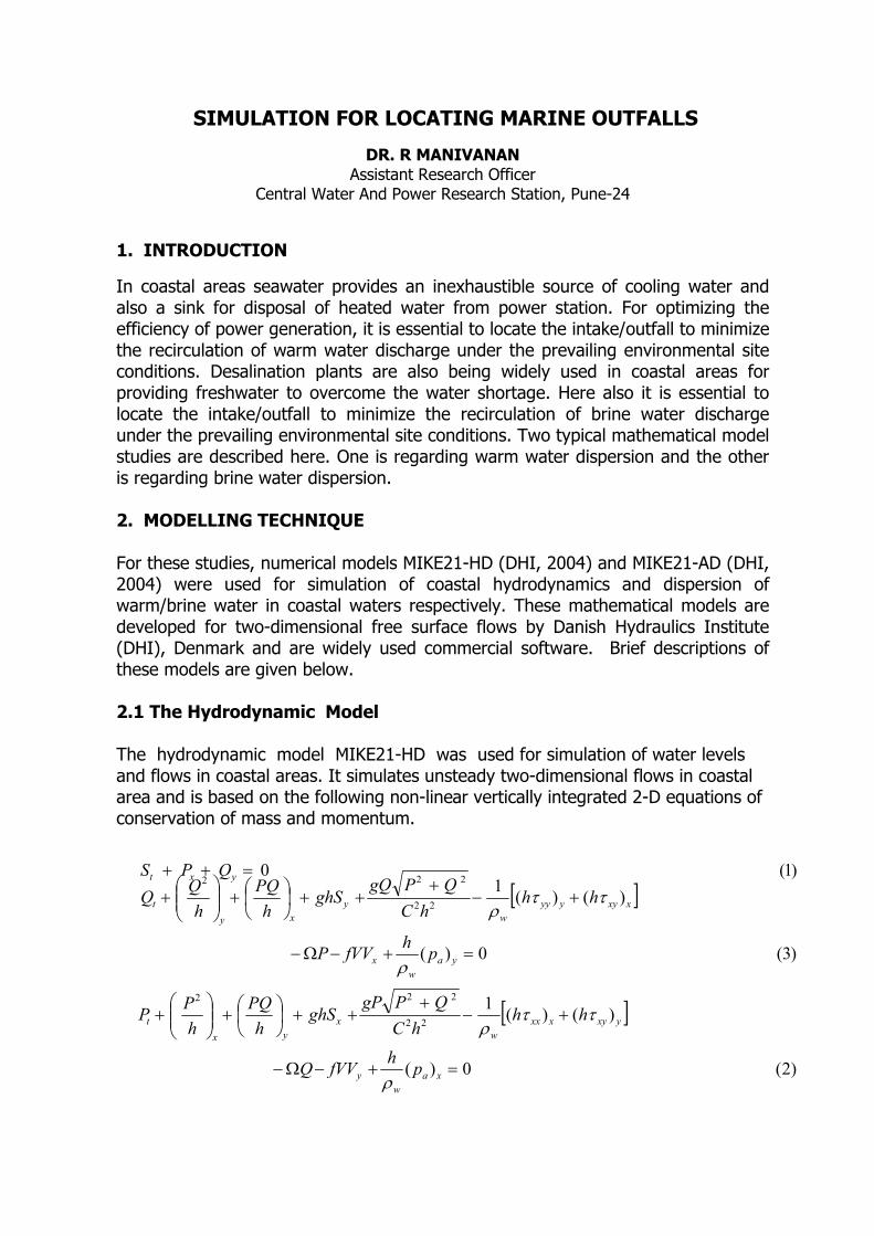
Fig. 1 : Index map water system for which the cooling water required for the power station (i.e. about 35 m3/s) is drawn from the sea through an intake well which is located at 360 m (Fig.1) from the shore and connected to the forebay of the pump-house by a submarine tunnel. An approach jetty is constructed for carrying out maintenance of the intake well. The warm water from the condensers with rise in temperature of 10 0C is discharged back to sea at the root of the approach jetty. Due to warm water discharge and littoral drift prevailing at the site, a sand-spit of about 2 km length parallel to the coast is formed (Fig.1). There is a proposal to establish a Prototype Fast Breeder Reactor (PFBR) of 500 MW capacity at 500 m south of MAPS. The cooling water requirement for this proposal would be 22 m3/s and the warm water from the condensers would be with a rise in temperature of 100 C. The intake structure of PFBR is to be located in the sea at 460 m from the shoreline and 680 m towards south from the MAPS intake structure (Fig.1). A suitable location of outfall for PFBR was to be determined to minimize warm water recirculation through the intakes, while both MAPS and PFBR projects are operating simultaneously. Mathematical model studies carried out for this purpose are described in this lecture. 3.1 Site Conditions Tides are semi-diurnal with maximum spring tidal range and minimum neap tidal range to be 1.22 m and 0.25 m respectively. The tidal currents are quite weak and do not exhibit any correlation with the tide or tidal phase. The currents are unidirectional. They are northerly during February to September with magnitude up to 0.5 m/s and southerly during October to January with magnitude of the order of 0.1. The current pattern (as well as thermal dispersion due to MAPS) at the site is also described in Gole et al (1975).



4

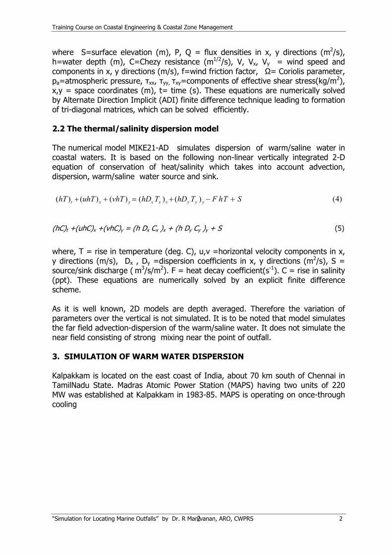
Due to combined action of the warm water discharge and the prevailing littoral drift of the order of 0.5 million m3 annually towards north, a sand-spit of about 2 km length parallel to the coast has formed. This has created a warm water channel between the shore and sand-spit. The length of the sand spit varies seasonally corresponding to the change in the magnitude and direction of the littoral drift. The ambient seawater temperature varies from 270 C to 320 C. The field studies in the region of the MAPS intake/outfall indicated that the thermal plume has a thickness of about 2 m from the surface (Anup Kumar, 1994) and has a tendency to get attached to the shore. The wind data of the site indicated that in general, during SW monsoon, wind blows predominantly from SW with intensity of about 13-17 m/s and during NE monsoon it blows predominantly from NE direction with the same intensity. 3.2 Model Operation The region considered for the model study is 2.5 km X 11 km with 50 m grid size, covering about 5.5 km on either side of the MAPS jetty and extending up to –15 m contour. The western side of the model region consists of the shoreline while the remaining sides are open to sea. Before using the model for predictive purpose, it is calibrated. The recirculation temperature limit is considered to be 10 C. However, it can be exceeded provided the recirculating water temperature is less than the design inlet seawater temperature of MAPS/PFBR which is 300/ 31.50 C respectively and/or duration of such increased temperature is for a short period. With this criteria for recirculation, several cases of outfall location were examined taking into consideration the seasonal changes in currents, length of outfall channel/ sand spit/guided bund etc. During 6-8 months (from February to September) the current direction is towards north with magnitude up to 0.5 m/s and during 3-4 months (October to January) the current direction is towards south with magnitude of the order of 0.1 m/s. Hence the model operation for northward current up to 0.5 m/s and for southward current of 0.1 m/s was considered. Several alternatives (Fig.2) were considered for studies, which are described below. Alternative A1 One of the alternatives considered for the PFBR outfall location is that the outflows from PFBR and MAPS to be let out through a channel parallel to coastline formed by construction of a guided bund. The channel would consist of a guided bund of 680 m length from PFBR outfall to MAPS outfall and would extend further towards north by some length. Trials for determining this extension were made and finally the optimum length of 500 m for the extension was determined by the model studies. In general, the model results indicated that the temperature plume (with temperature rise more than 1 0 C ) is shore attached extending along the shore



5

towards north/south for about more than 5 km and towards south/north for about 500-600 m from the point of outfall in the sea and the cross-shore spread was of the order of about 900 m from

) Fig. 2 : Alternatives of PFBR outfall (Schematic

the shore for the northward/southward current of the order of 0.1 m/s. Increase in thecurrent magnitude causes increase in the longshore spread while the cross-shore spread decreases considerably. During the period of northward current no recirculation was predicted while during southward current some recirculation may occur. Alternative A2 In order to avoid recirculation during the period of southward current, this alternative is considered. The outflows from PFBR and MAPS to be let out through a channel parallel to coastline formed by constructing a guided bund. As in the case of Alternative A1, the channel would consist of a guided bund of 680 m length from the PFBR outfall to MAPS outfall and would extend further towards north by 500 m. In addition, it is being extended from PFBR outfall towards south by some suitable length. With the arrangement of gates the outflows from MAPS and PFBR would be let out through the channel to the north side during the period of northerly current and to the south side during the period of southerly current. The optimum length of the southward extension was determined to be 300 m from the model studies. In this case, care has to be taken regarding operation of the gates. Alternative B Another option is to take PFBR outflow along a jetty perpendicular to the coastline and discharge into deep sea at some distance from the shore. Trials were made to

680m

MAPS PFBR

(A1) 500m

N

680m (A2) 500m 300m

680m

MAPS

PFBR OUTFALL

(B)750m

G

MAPS PFBR

• INTAKE

OUTFALL GATE

G

460m360m

460m 360m

360m 460m

GUIDE BUND

G



6

determine the optimum distance from the shore, which was found to be 750 m. Fig. 3 shows typical thermal flow field for northward and southward currents of the order of 0.1 m/s. The longshore and cross-shore spread of the plume was observed to be similar to the case of Alternative A1.

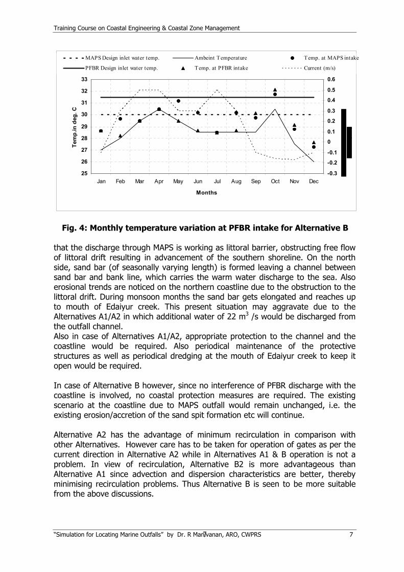
Fig. 3 : Dispersion of warm water in Alternative B In order to get an idea about the possibility of recirculation of warm water at the intakes, the monthly temperature variations at the MAPS and PFBR intakes were examined (Fig.4). It is seen that during April and October the ambient temperature itself is more than the design inlet water temperature of MAPS (i.e. 300 C). The maximum rise in temperature at the intakes is of the order of 1.50 C above the ambient temperature. Therefore there is a possibility that the water temperature at the intakes would be higher by about 1-1.50 C than the design inlet water temperature for a short duration when the ambient temperature itself is high and the currents are weak. MAPS have been commissioned in the years 1983-1985. Since then the warm water from MAPS (35 m3/s) is being discharged into the sea from the bank line. It is seen

Current

Current



7

25

26

27

28

29

30

31

32

33

Jan Feb Mar Apr May Jun Jul Aug Sep Oct Nov Dec

Months

Tem

p.in

deg

. C

-0.3

-0.2

-0.1

0

0.1

0.2

0.3

0.4

0.5

0.6

MAPS Design inlet water temp. Ambeint Temperature Temp. at MAPS intake

PFBR Design inlet water temp. Temp. at PFBR intake Current (m/s)

Fig. 4: Monthly temperature variation at PFBR intake for Alternative B that the discharge through MAPS is working as littoral barrier, obstructing free flow of littoral drift resulting in advancement of the southern shoreline. On the north side, sand bar (of seasonally varying length) is formed leaving a channel between sand bar and bank line, which carries the warm water discharge to the sea. Also erosional trends are noticed on the northern coastline due to the obstruction to the littoral drift. During monsoon months the sand bar gets elongated and reaches up to mouth of Edaiyur creek. This present situation may aggravate due to the Alternatives A1/A2 in which additional water of 22 m3 /s would be discharged from the outfall channel. Also in case of Alternatives A1/A2, appropriate protection to the channel and the coastline would be required. Also periodical maintenance of the protective structures as well as periodical dredging at the mouth of Edaiyur creek to keep it open would be required. In case of Alternative B however, since no interference of PFBR discharge with the coastline is involved, no coastal protection measures are required. The existing scenario at the coastline due to MAPS outfall would remain unchanged, i.e. the existing erosion/accretion of the sand spit formation etc will continue. Alternative A2 has the advantage of minimum recirculation in comparison with other Alternatives. However care has to be taken for operation of gates as per the current direction in Alternative A2 while in Alternatives A1 & B operation is not a problem. In view of recirculation, Alternative B2 is more advantageous than Alternative A1 since advection and dispersion characteristics are better, thereby minimising recirculation problems. Thus Alternative B is seen to be more suitable from the above discussions.



8

3.3 CONCLUSIONS From this mathematical model study, the following conclusions are drawn. 1. Alternative A2 has the advantage of minimum recirculation in comparison with other Alternatives. However care has to be taken for operation of discharge as per the current direction in Alternative A2 while in Alternatives A1 & B operation is not a problem. 2. With the Alternative A1 & A2, appropriate protection to the channel and coastline would be needed and periodical maintenance of the protective structures will have to be carried out. Also, periodical dredging would be required to keep open the mouth of Edaiyur creek. 3. Alternative B has the following advantages over Alternatives A1 & A2.

• Advection and dispersion characteristics are better, thereby recirculation problems are minimized.

• No interference of outfall water with the coastline. The existing scenario at the coastline due to MAPS outfall would remain unchanged.

• No impact on Edaiyur creek mouth • MAPS outfall and PFBR outfall would be independent of each other thereby

minimizing the interaction of the two. Hence the Alternative B is preferable compared to Alternative A1 & A2.

4. With Alternative B the intake may be suitably designed for selective withdrawal of cold water since the warm water plume extends up to 2 m from the water surface. 4. SIMULATION OF BRINE WATER DISPERSION

Chennai Petroleum Corporation Ltd (CPCL) has installed a 5.8 MGD sea water Desalination Plant at Ennore at about 25 km north of Chennai in Tamilnadu to cater for their existing refinery. The intake and outfall system of the plant is located at about 2-3 km north of the Ennore port. The layout of intake and outfall of the plant is shown in Fig. 5. Sea water is taken from the intake well at about 350 m from the shore and the brine water discharge coming out from the plant is let out in the sea through pipeline at the outfall location at about 750 m from the shore. The sea water requirement of the plant would be going to be doubled to 12 MGD in the near future.

Larsen and Toubro(L & T) along with Tamilnadu Industrial Development Corporation (TIDCO) is developing a Shipyard cum Port facility at Kattupalli which is about 3-4 km north of Ennore port (Fig.5). The existing intake/outfall system of Chennai Petro Chemicals Ltd (CPCL) is falling within the proposed harbour basin of the Shipyard cum Port facility at Kattupalli. It is proposed to relocate the CPCL intake and outfall outside the port basin on the south side of the south breakwater such that there would be minimum recirculation in the intake. Mathematical model studies were carried out for determining suitable locations of the intake/outfall of



9

CPCL during temporary stages of construction of breakwaters and permanently outside the proposed port basin.

Fig. 5: Existing Locations of Intake & Outfall

4.1 MODEL OPERATION The region considered for the model is about 8.5 km X 11.5 km covering about 5.75 km on the either side of the proposed port and extending up to about -27 m contour. The western side of the model region consist the shoreline while the remaining sides are open to sea. The mathematical model studies were to be carried out taking into account construction stages of the north and south breakwaters (i) with existing locations of intake and outfall (ii) with existing location of intake and temporary location of outfall on the south side of the south breakwater (iii) with the permanent locations of intake and outfall outside the proposed port basin. Accordingly three scenarios

2 -10

-15

-20 -25

2

-10 -15

-20

-25

2 -8 -15

-25

2 -5 -10 -15

-25

2 -8 -20 -25

2

-8 -10

-20

-25

2

-8 -10-15

-25 -29

2 -10 -15 -25

2 -10 -15

-25

2 -10 -15

-25

Untitled (meter)Above 10

2 - 10-2 - 2-3 - -2-5 - -3-8 - -5

-10 - -8-15 - -10-20 - -15-25 - -20-29 - -25-35 - -29-40 - -35-45 - -40

Below -45

01/01/2002 00:00:00

0 20 40 60 80 100 120 140 160(Grid spacing 50 meter)

0

10

20

30

40

50

60

70

80

90

100

110

120

130

140

150

160

170

180

190

200

210

220

230(G

rid s

paci

ng 5

0 m

eter

)

Intake Outfall



10

of the intake and outfall of CPCL are considered for the mathematical model operation namely Existing, Temporary and Permanent. The ambient temperature of sea water is assumed to be 270C. Ambient salinity of sea water is assumed to be 32 ppt. The rise in salinity of brine water to be discharged at the outfall is given to be 31 ppt above ambient. For the salinity model, as the open boundaries have been taken sufficiently away from the outfall locations, zero rise in salinity is assumed at the open boundaries. It is observed that in the open sea at the site, the flow is unidirectional, either northerly or southerly generally parallel to the coastline. During the period February-September the flow is northward, while during the period October-January the flow is southward. The model is operated for different current conditions namely northward 0.25 m/s, southward 0.25 m/s and weak current i.e. 0.05 m/s. The direction of the weak current is considered to be northward or southward depending on the locations of intake and outfall to simulate the critical condition. In order to maintain efficiency of the desalination plant, the recirculation of salinity in the intake should be avoided by selecting proper locations of intake and outfall. For avoiding the recirculation the limiting salinity rise at the intake above ambient is considered as 0.1 ppt. Existing Scenario: The model was operated with existing locations of intake and outfall enclosed by the proposed north and south breakwaters with outfall discharge of 0.312 m3/s with length of both north & south breakwaters extended up to 200 m, 500m. With length of breakwaters = 200 m The model was first operated with lengths of both north and south breakwaters = 200 m with northward and southward average current of 0.25 m/s. The model was operated for 15 days period. As expected, the brine water was dispersing without much significant effect due to the 200 m long breakwaters. The time history of salinity rise indicated oscillations in salinity rise according to tidal phase. The average salinity rise at the outfall was of the order of 0.35 ppt and the average salinity rise at the intake was less than 0.1 ppt. The model was further operated with lengths of both north and south breakwaters = 200 m and for weak current of 0.05 m/s. It was seen that after 15 days, dispersion of salinity is very slow with average salinity rise at the intake and outfall to be of the order of 0.25 ppt and 0.6ppt respectively. This situation of weak current may occur for short period less than 15 days in a year. With length of breakwaters = 500 m The model was operated with lengths of both north and south breakwaters = 500 m with northward and southward average current of 0.25 m/s. The model was operated for 15 days period. The brine water was dispersing without much significant effect due to the 500 m long breakwaters. The average salinity rise at



11

the outfall was of the order of 0.35 ppt and the average salinity rise at the intake was less than 0.1 ppt.(Fig.6) The model was further operated with lengths of both north and south breakwaters = 500 m and for weak current of 0.05 m/s. It was seen that after 15 days, dispersion of salinity is very slow with average salinity rise at the intake and outfall to be of the order of 0.35 ppt and 8 ppt respectively.

(Southward Current) (Northward Current) Fig. 6: Distribution of Rise in Salinity at LW Slack After 15 Days, Exisitng Scenario : Length of North & South Bws=500m Thus the construction of both north and south breakwater can progress to 500m without any interference to intake water salinity. Temporary Scenario The model was operated with outfall discharge of 0.312 m3/s for the Temporary Scenario i. e. for the existing location of intake inside the harbour and temporary location of outfall outside the harbour on south side of the south breakwater as shown in Fig 7. The model was run with the stages of construction of north and south breakwaters with lengths = 500 m, 750m and 1000m. The model was operated for northward and southward average current of 0.25 m/s, and weak current i.e. 0.05 m/s.



12

Fig. 7: Temporary Scenario with North & South BW=1000 M With length of breakwaters = 500 m In this case the average salinity rise at the outfall was of the order of 1.5 ppt. The average salinity rise at the intake was of the order of 0.15 ppt and 0.06 ppt for northward and southward currents respectively. This situation of 500 m breakwaters may exist for a period of 2-3 months after which the breakwaters would be extended further. For weak current. the average salinity rise at the intake and outfall was of the order of 0.3 ppt and 2.0 ppt respectively. This situation of weak current may occur for a short period less than 10-15 days in a year. With length of breakwaters = 750 m In this case, the model results indicated that the average salinity rise at the outfall is of the order of 1.7 ppt. The average salinity rise at the intake is of the order of 0.12 ppt and 0.04 ppt for northward and southward currents respectively. This situation of 750 m breakwaters may exist for a period of 2-3 months after

Untitled [-]Above 7.5

5 - 7.52.5 - 5

0 - 2.5-2.5 - 0

-5 - -2.5-7.5 - -5-10 - -7.5

-12.5 - -10-15 - -12.5

-17.5 - -15-20 - -17.5

-22.5 - -20-25 - -22.5

-27.5 - -25Below -27.5Undefined Value

0 20 40 60 80 100 120 140 160(Grid spacing 50 meter)

0

10

20

30

40

50

60

70

80

90

100

110

120

130

140

150

160

170

180

190

200

210

220

230

(Grid

spa

cing

50

met

er)

Untitled

INTAKE

OUTFALL



13

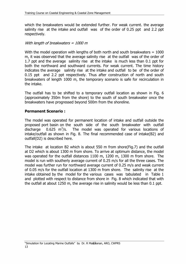
which the breakwaters would be extended further. For weak current. the average salinity rise at the intake and outfall was of the order of 0.25 ppt and 2.2 ppt respectively. With length of breakwaters = 1000 m With the model operation with lengths of both north and south breakwaters = 1000 m, it was observed that the average salinity rise at the outfall was of the order of 1.7 ppt and the average salinity rise at the intake is much less than 0.1 ppt for both the northward and southward currents. For weak current. The time history indicates the average salinity rise at the intake and outfall to be of the order of 0.15 ppt and 2.2 ppt respectively. Thus after construction of north and south breakwaters of length 1000 m, the temporary scenario is safe for recirculation in the intake. The outfall has to be shifted to a temporary outfall location as shown in Fig. 6 (approximately 350m from the shore) to the south of south breakwater once the breakwaters have progressed beyond 500m from the shoreline. Permanent Scenario : The model was operated for permanent location of intake and outfall outside the proposed port basin on the south side of the south breakwater with outfall discharge 0.625 m3/s. The model was operated for various locations of intake/outfall as shown in Fig. 8. The final recommended case of intake(B2) and outfall(D2) is described here. The intake at location B2 which is about 550 m from shore(Fig.7) and the outfall at D2 which is about 1300 m from shore. To arrive at optimum distance, the model was operated for the outfall distances 1100 m, 1200 m, 1300 m from shore. The model is run with southerly average current of 0.25 m/s for all the three cases. The model was further run for northward average current of 0.25 m/s and weak current of 0.05 m/s for the outfall location at 1300 m from shore. The salinity rise at the intake obtained by the model for the various cases was tabulated in Table 1 and plotted with respect to distance from shore in Fig. 8 which indicated that with the outfall at about 1250 m, the average rise in salinity would be less than 0.1 ppt.



14

Fig. 8 : Permanent Intake/Outfall Locations TABLE 1 : RISE IN SALINITY ABOVE AMBIENT FOR PERMANENT SCENARIO WITH INTAKE AT B2 & OUTFALL D2

Rise in salinity (ppt) above ambient S. No

Outfall distance from shore(m)

Current Range Average

1 1100 Southward 0.00-0.30 0.15 2 1200 Southward 0.00-0.22 0.11 3 1300 Southward 0.00-0.17 0.08 4 1300 Northward 0.00-0.09 0.04 5 1300 Weak 0.00-0.50 0.40

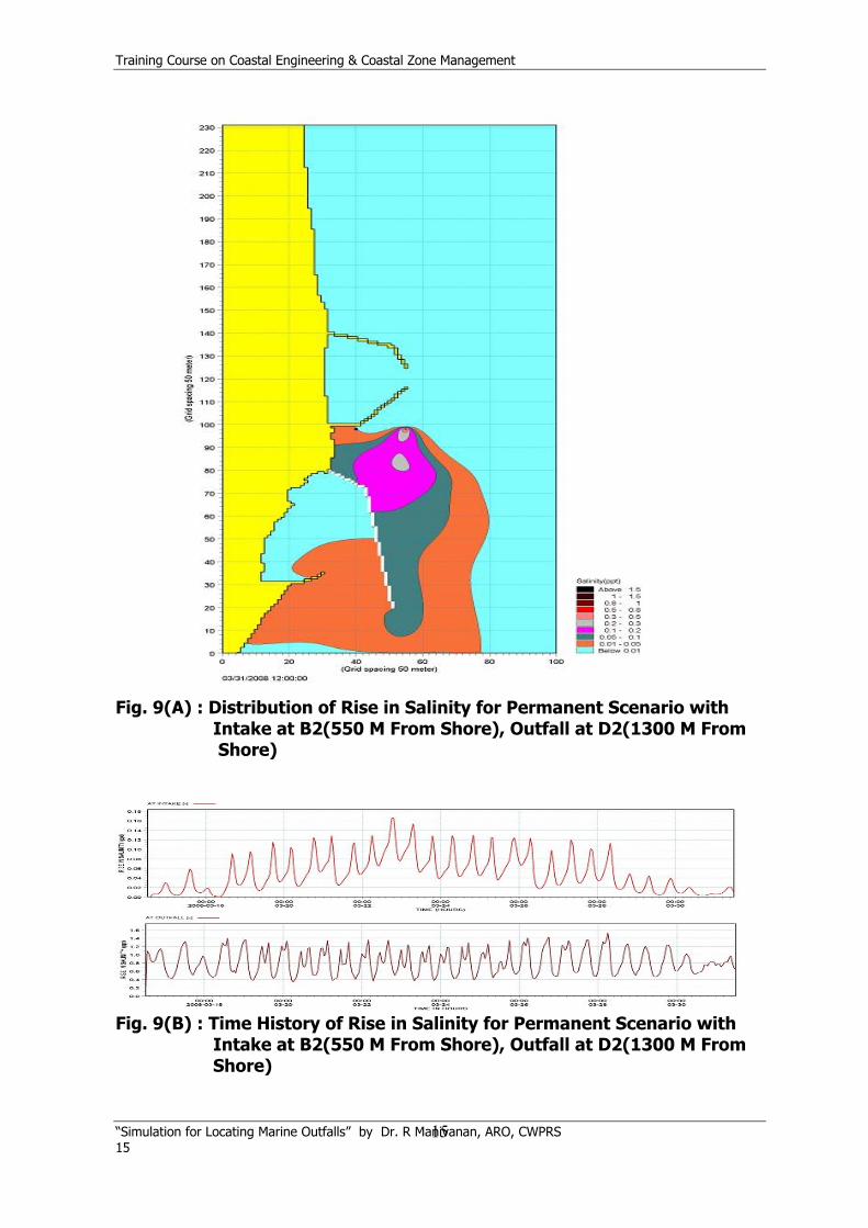
Typically, distribution of salinity rise and time history at intake and outfall for outfall distance of 1300 m from shore are shown in Figs.9(A, B).

B1

B2

D1

2

A1

1500 m

1300 m

550 m 700 m

A1, A2, B1, B2 : INTAKE LOCATIONS D1, D2 : OUTFALL LOCATIONS

D2



15

Fig. 9(A) : Distribution of Rise in Salinity for Permanent Scenario with Intake at B2(550 M From Shore), Outfall at D2(1300 M From Shore)

Fig. 9(B) : Time History of Rise in Salinity for Permanent Scenario with Intake at B2(550 M From Shore), Outfall at D2(1300 M From Shore)



16

4.2 CONCLUSIONS

1. The construction of both north and south breakwater can progress to 500m without any interference to intake water salinity

2. The outfall has to be shifted to a temporary outfall location as shown in Fig. 6 (approximately 350m from the shore) to the south of south breakwater once the breakwaters have progressed beyond 500m from the shoreline.

3. The permanent locations of intake and outfall relocation outside the port basin with the intake at B2 (approximately 550m from the shoreline) and outfall at D2 (approximately 1300 m from shoreline) as shown in Fig. 8 would be suitable to avoid brine recirculation in the intake.

5 REFERENCES Anup Kumar B., Rao T. S., Venugopalan V.P. and Narasimhan S.V, 2002,

Thermal mapping in the Kalpakkam coast (Bay of Bengal) in the vicinity of Madras atomic Power station, Int. Conf. On Hydrology and watershed Management with a Focal Theme on water quality and Conservation for sustainable development (ICHWAM-2002), held at JNTU, Hyderabad.

Danish Hydraulic Institute, 2004, MIKE21-HD, Coastal Hydraulics and

Oceanography – Hydrodynamic Module, User’s guide and reference manual. Danish Hydraulic Institute, 2004, MIKE21-AD, Environmental Hydraulics –

Advection Dispersion Module, User’s Guide and reference manual. Gole, C V., Tarapore, Z S and Parcure, T M (1975) “Thermal discharges into

the marine environment- Model studies for Madras Atomic Power Project, Kalpakkam”. Proc. of 4th Annual Research Session of CBIP Publication no.123, Paper no.4.

simulation for locating marine...

Documents