i

Simulation of coordinated traffic light control using model predictive control

Wieberen Kooistra Research paper Business Analytics August 2012 Supervised by Sandjai Bhulai

ii

Preface This research paper is a compulsory part of the Master program Business Analytics at VU University Amsterdam. The purpose of the paper is to do research on a subject that is related to business, computer science, and mathematics. The main purpose of this paper is a simulation of traffic light control in a network of intersections. This is done with Model Predictive Control (MPC). I would like to thank my supervisor, Sandjai Bhulai, for the advice and support he gave me during the programming stage and for the feedback he gave me during the writing stage. I also want to thank Sjoerd Linders from the planning service department of Amsterdam for the information and data he gave me of the traffic lights in Amsterdam.

iii

Summary There is a lot of traffic in urban areas, which can lead to long traffic jams and large traffic delays. To reduce these problems it is important that there is good traffic light control. Traffic light control can be done by isolated or coordinated control. Isolated control is used for the control of a single intersection and coordinated control is used for the control of a network of intersections. An example of coordinated control is Model Predictive Control (MPC). MPC uses a prediction model to determine the future traffic states, and an optimization algorithm uses these traffic states to determine the optimal traffic control for the next period. When there is real-time data available a rolling horizon approach can be used to update the begin states. In this paper the BLX model is described, this a prediction model that can be used for the MPC controller. When the BLX model is used as prediction model for the MPC method, a binary non-linear optimization problem with the total waiting time as objective function and the constraints of the model as constraint should be solved to control the traffic lights. This optimization problem is solved with a heuristic approach. The goal of this paper is to see what the pros and contras of the BLX model and the chosen heuristic are. To do this the following main question will be answered: Is the BLX model a reliable and fast model to use for Model Predictive Control? What is the influence of changing different input parameters of the model? Is the used heuristic approach a good way to solve the optimization problem? With a simulation model and a dataset from a row of intersection at the Wibautstraat in Amsterdam different tests are performed to give an answer to the above questions. For the heuristic approach two methods to determine the order of the lights are compared with each other; the simple and fast method give almost the same results as the extensive and slow method. And thus the simple method is used for the other test. The intersections at the Wibautstraat all have a cycle time of 66 seconds, to see if this is the optimal value the model is run with different cycle times. The graph with results has a u-shape with 60 seconds as minimum. When the cycle time is higher, the lights at one intersection cannot react fast on the lights at other intersections and when the cycle time is lower the green time period of the green wave becomes lower. To be sure that all lights are green once during a cycle time a minimum green time length is set. The total waiting time is the lowest when there is a minimum of one and it grows when the minimum grows, but when the minimum is four the waiting time is lower then at three and five. A minimum of one is the best, but then the cars at the queue have not enough time to leave, so the optimal minimum time will set to four seconds. The BLX model is a fast model, but when you use an extensive approach in the optimization part it becomes slower. When you use the model in a real time situation is should be very fast to use it. So if you use the BLX model with a simple method to solve the optimization problem it is suitable to use, but when the model has run a lot of times in the optimization part it is not fast enough. The results using the heuristic approach are compared with the real results and the results have the same pattern. They are not exact the same, but a reason for this could be the fact that the used methods in practice also have to deal with other road users. The heuristic approach does not give the globally optimal solution but it gives a good local solution.

iv

Table of Contents 1. Introduction .............................................................................................................................................. 1

2. Prediction model ....................................................................................................................................... 3

2.1 BLX Model ....................................................................................................................................... 3

2.2 Extended model .............................................................................................................................. 5

3. Model Predictive Control .......................................................................................................................... 7

3.1 Prediction model ............................................................................................................................. 7

3.2 Optimization problem ..................................................................................................................... 7

3.3 Rolling horizon ................................................................................................................................ 8

4. Simulation ................................................................................................................................................. 9

4.1 Input ................................................................................................................................................ 9

4.2 Simulation model ............................................................................................................................ 9

4.3 Assumptions .................................................................................................................................... 9

4.4 Intersection structure ..................................................................................................................... 9

4.5 Traffic light constraints ................................................................................................................. 10

5. Optimization problem ............................................................................................................................. 11

5.1 Heuristics ....................................................................................................................................... 12

6. Traffic light control in Amsterdam .......................................................................................................... 13

7. Results ..................................................................................................................................................... 16

7.1 Order of the lights ......................................................................................................................... 16

7.2 Different cycle times ..................................................................................................................... 17

7.3 Boundaries .................................................................................................................................... 18

7.4 Green Wave .................................................................................................................................. 19

8. Conclusion and further research............................................................................................................. 19

9. References .............................................................................................................................................. 20

1

1. Introduction In large cities there is a lot of traffic, which can lead to traffic jams and large traffic delays. This is not favourable for the environment, it decreases the safety of road users, and for companies it could be a reason to move to a city that is better reachable. To reduce the waiting time of cars, the infrastructure of a city could be improved by building new roads or by changing existing roads. But this could be expensive and it is limited by the existing geography of cities. An easier and cheaper way to reduce the traffic problem is by traffic light control. When you use this in a good way it can lead to a better traffic flow, which reduces the waiting times. Traffic light control can be done in different ways; you can use isolated control or coordinated control. Isolated control is used for the control of a single intersection and coordinated control is used in urban areas to control a network of intersections. When you use coordinated control, the intersections in a specified area interact with each other. This is good for the traffic flow of the cars and reduces the overall waiting time, but the implementation of this is complicated. If you use one of these control mechanisms an algorithm that determines the optimal state of a traffic light at each time step is needed. There are already some traffic control algorithms developed [3]. These can be divided into fixed-time algorithms and traffic response algorithms. Fixed time algorithms use historical data to make a fixed planning for the traffic lights for a specified future period. Traffic response algorithms interact with sensors that measure the number of cars that are waiting at the intersections, and it uses these real-time measures to control the traffic lights. Model Predictive Control (MPC) uses real time data to predict future traffic states. These future traffic states are found with a prediction model, and then the optimal traffic control for the next period is determined using an optimization algorithm and the traffic states for this period. Different prediction models and optimization algorithms could be used for this control method. An example of a prediction model is the BLX model of Lin, Schutter, Xi and Hellendoorn [2], with this model the number of cars that arrive and leave at the intersection at each time step can be calculated and it calculates the total time that all cars are waiting in the traffic network. When the BLX model is used as prediction model for the MPC method, a binary non-linear optimization problem with the total waiting time as objective function and the constraints of the model as constraint should be solved to control the traffic lights. For this paper a simulation program is made, which uses the BLX model as basis. To make it easier to work within the simulation some changes on the model are made. The simulation program solves the optimization problem with a heuristic approach. This paper gives an explanation of the BLX model and the use of Model Predictive Control. After that it gives a description of the simulation program and how it is used to find an answer for the following main questions: Is the BLX model a reliable and fast model to use for Model Predictive Control? What is the influence of chancing different input parameters of the model? Is the used heuristic approach a good way to solve the optimization problem?

2

To test if the BLX model is a good and fast model and to see what the impact of different parameters is, a dataset of a network of intersections in Amsterdam is used. This dataset is also used to see if the heuristic approach gives good results. These tests are also used to optimize the heuristic approach.

3

2. Prediction model When you use a model predictive control (MPC) approach for controlling and coordinating a traffic network, a fast model with low online computational complexity is needed. As basis for this model, the BLX model of Lin, Schutter, Xi and Hellendoorn[2] is used. In this model the simulation time step is set to one second and all variables are updated at each step. To reduce the computational time a few changes are made on this model.

2.1 BLX Model

To describe the BLX model some notation for this model is introduced. J = set of nodes (intersections) L = set of links (roads) (u,d) = link with upstream node u (u J) and downstream node d (d J) Iu,d = set of input nodes of link (u,d) Ou,d = set of output nodes of link (u,d) k = simulation step counter nu,d(k) = number of vehicles in link (u,d) at step k qu,d(k) = queue length at step k in link (u,d) qu,d,o(k) = queue length at step k in link (u, d) of the sub-stream turning to link o

= number of cars leaving link (u,d) at step k and turning to o

= number of cars arriving at the end of the queue in link (u,d) at step k

= number of cars arriving in the sub stream towards o in link (u,d) at step k

= flow rate arriving at the end of the queue in link (u,d) at step k

= arriving flow rate of the sub-stream towards o in link (u,d) at step k

Su,d(k) = available storage space of link (u,d) at step k expressed in number of vehicles = relative fraction of the traffic in (u,d) turning to link o at step k

µu,d = saturated flow rate leaving link (u,d) gu,d,o(k) = Boolean value indicating whether the traffic signal at intersection d for the traffic

stream in link (u,d) turning to o is green (1) or red (0) at step k

= free flow vehicle speed in link (u,d)

Cu,d = capacity of link (u,d) expressed in number of vehicles

= number of lanes in link (u,d)

lveh = average vehicle length cu = cycle time for intersection u Ts = Simulation time step = time to drive, expressed in simulation time steps, from the beginning of the link to the

end of the queue at step k, rounded to an lower integer. = Exact time to drive, expressed in simulation time steps, from the beginning of the link

to the end of the queue at step k minus .

4

Fig. 1 A link connecting two traffic signal controlled intersections.

In the BLX model a queue is modelled as follows. For each destination a separate queue is constructed. The simulation time step Ts is set to one second and cars arriving at the end of a queue in simulation period [kTs,(k+1)Ts] are allowed to cross the intersection in that same period (if their traffic light is green, there is enough free space in the outgoing link, and there are no other restrictions). Consider link (u,d), for each outgoing link o Ou,d the number of cars leaving link (u,d) for destination o in the period [kTs,(k+1)Ts] is given by

.

There are only cars leaving the queue when the traffic lights is green, otherwise the number of leaving cars is zero. When the traffic light is green, the number of cars leaving the link (u,d) depends on the number of cars waiting and arriving at the queue, the available space in the outgoing link, and the saturated flow rate during the period. These three variables are all upper bounds for the number of cars leaving the link. Then the number of leaving cars is the minimum of these three variables. The traffic arriving at the end of the queue in link (u,d) at time step k is given by the traffic entering the link via the input links delayed by the time needed to drive from the beginning of the link to the end of the queue in the link. So the fraction of cars that arrive at the queue at step k and enters the link at step is equal to ). And the fraction of cars that arrive at the queue at step k and enters the link during step is 1 . The number of cars arriving is calculated by the sum of cars that leaves the input links at simulation step and the sum of cars that leave the input links at step .

,

where

,

5

.

is the number of simulation steps that it takes to drive from the beginning to the end of the link. Floor(x) is used to round to the largest integer smaller than or equal to x. is the remainder of the number of simulation steps. Rem(x) is the remainder of x. The number of arriving cars in link (u,d) turning to o Ou,d is the number of arriving cars at the end of the queue in link (u,d) multiplied by the relative fraction that turns to link o.

.

The new queue lengths at link (u,d) for each o Ou,d are given by the old queue lengths plus the arriving traffic minus the leaving traffic

.

The new available storage of link (u,d) is given by the old available storage minus the number of cars that enters the link (u,d) plus the number of cars that leaves the link (u,d) in the period [kTs,(k+1)Ts]:

.

2.2 Extended model

In the extended model a difference is made between the location of a link in the network: there are incoming, outgoing and network links. An incoming link is a link that only has output links (no input links), an outgoing link is a link that has only input links and a network link is a link that has input and output links (lies between two intersections).

Each incoming link has a pre-defined arrival rate , and the number of arriving cars at queue

qu,d,o,is calculated each time the status of the traffic light changes (from red to green or from green to red). The number of arriving cars is calculated by the arrival rate multiplied with the length of the interval.

.

When the traffic light changes from red to green, the interval is [time – begin red period]. When the lights change from green to red, the interval is [time – begin green period]. The number of arriving cars at a network link is calculated in the same way as in the BLX model. So in case of a network link the number of arriving cars is still updated every second, but in case of an incoming link it is only updated when there is change of the status of the traffic lights. This reduces the computation time. The intersections in the network could have different cycle times and the control time interval is adopted by all the intersections in the network, with Nj an integer, as Tctrl = Nj *cj for all j J. So Tctrl is the least common multiple, of all the intersection cycle times in the traffic network.

6

3. Model Predictive Control Model Predictive Control is a model-based optimization control method for urban traffic networks. The MPC method applies Optimal Control in a rolling horizon way. At each step only the first part of the optimal control solution is used. Then the horizon is shifted one step forward and then the optimization is started again with new information of the measurements. The optimization is based on the prediction model of the process and an estimate of the future traffic disturbance. The advantages of MPC are that it can deal with the uncertainty of the process, which can be caused by the unpredictable disturbance, changing parameters over time and model mismatches in the prediction model. Another advantage is that you can easily change the prediction model. The MPC framework has three typical features: The prediction model, optimization of the control input, and the rolling time horizon. These three steps can be described as follows:

1) 3.1 Prediction model The MPC controller uses a prediction model to predict the future traffic states, which can be used to calculate the objective function. The model predicts these traffic states based on information of current states, predicted disturbances and future control inputs. In the previous chapter the BLX model is described, this is an example of a prediction model. The prediction of future traffic states can be described as , where n(k) is the traffic state (number of vehicles in a link at time step k); d(k) is the predicted disturbance; g(kc) is the future control input (green time of the traffic lights)

2) 3.2 Optimization problem For a given control time interval Tctrl and a given simulation interval Ts, we have Tctrl = M*Ts, where M is the number of stimulation steps that fits in one control interval. In each step we predict the future traffic states for the prediction horizon Np. Np is a number of control time intervals. So the number of simulation steps in the prediction horizon is equal to Np * M. The future traffic states are predicted at simulation time step k as

.

These are based on the predicted traffic demands at simulation time step k

,

and on the future traffic control input (status of the lights) at control step kc

.

The total queue length in a link is give by ql.

7

The Total Waiting Time at the queues (TWT) is chosen as objective function then the optimization problem becomes:

,

s.t. model constraints, s.t. traffic light constraints. The model constraints are all the constraints of the used prediction model. The traffic light constraints are needed to handle the traffic control in a good way. For example lights that disturb each other could not be green at the same time. In the optimization chapter these constraints will be described. Because g(kc) is a binary matrix this is a binary non linear optimization problem, such problems cannot be solved exactly. The optimization problem can be rewritten to a tractable non-linear problem or to a MILP problem to solve it in an exact way. Or a heuristic approach can be used to get a locally optimal solution.

3) 3.3 Rolling horizon When the optimization problem is solved with a SQP algorithm the optimal control input g*(kctrl) is found. The first part of this control input g*(kctrl| kctrl) is the input for the prediction model. In the next control step kc +1 the prediction model gets real measured traffic states and the prediction horizon is moved one step forward. Then this whole process is repeated again. This rolling horizon approach enables the system to get feedback from the real traffic network; this makes the MPC controller robust to the uncertainty of the future traffic flows.

8

4. Simulation A simulation model is built that implements the described prediction model and a model predictive controller is built that uses this simulation model and an optimization algorithm to optimize the traffic light control.

4.1 Input

The input parameters of the MPC are:

- Hashtable with intersections, - Hashtable with links, - Hashtable with lights, - Number of control intervals, - Vehicle length.

With the cycle times of the intersections the length of a control interval is calculated. And then the optimal traffic control input, the status of each traffic light at each second, for the next control interval are defined using an optimization method. A heuristic method is implemented, but other methods can be easily implemented.

4.2 Simulation model

When the traffic control input for the next control interval is found the prediction model is started. The input parameters of this model are:

- Hashtable with intersections, - Hashtable with links, - Hashtable with lights, - Traffic control input, - Current control interval, - Vehicle length, - Length of control interval.

With the traffic control input an event list is made, the event list contains three different events:

- Red, when a traffic light changes from green to red an event with type Red is made. - Green, when a traffic light changes from red to green an event with type Green is made. - Arrival, when a car enters a network link an arrival event is made. This arrival event describes

the arrival of this car at the queue of one the lights at this link. So after handling the control input the event list is filled with red and green events for the whole control interval. Then, using a step size of one second, all events in the list are processed. The actions that are done depend on the type of the event; there are again three different choices.

- Red, first the number of arriving cars in the period that the light was green is determined; the method of calculating the arriving cars depends on the type of the link. This number is rounded up or down, both with probability 0.5. Then the number of cars that leave the link is calculated. This number is also rounded up or down with probability 0.5. With these data the new queue length, capacity and number of vehicles in the link are updated. When the outgoing link is a network link, new arrival events are made. After this the total waiting time is updated, using the number of cars that are in the queue during the past interval.

9

- Green, when the lights change from red to green, the light was red in the previous interval. So there are only arriving cars, these are calculated in the same way as in the case of a red event. Now again the new queue length, capacity and the number of vehicles in the link are updated, and the total waiting time during the interval is calculated.

- Arrival, when there is an arrival event, a car in a network link arrives at one of the three queues in that link. The queue length for the traffic light is updated.

4.3 Assumptions

To avoid that the model becomes too complex the following assumptions are made:

- The arrival rate from cars from outside the network is deterministic.

- Cars in the network have a constant speed.

- When a traffic light becomes green it takes one second before the first car leaves the queue.

- The cars in the network only leave it using the outgoing links.

- The cars in the network only arrive using incoming links.

- If a light at the begin of a network link is green at the same time as the light at the end of the

corresponding network link, the leaving cars at the beginning will not arrive at the queue at the

end of that link during the green time period. So we assume that the distance between these

two intersections is big enough to avoid this problem.

- There is a minimum and a maximum time a light is green during a control interval, these are

equal for all lights.

- The cycle times of all intersections are equal.

4.4 Intersection structure

For the model we use the following structure for an intersection. On each incoming and network link there are three traffic lights, traffic can turn to left or right or can go straight. Each intersection with four incoming links has in total twelve different traffic lights. Such an intersection is called an F12C4 intersection[1]. The twelve different traffic lights are divided into four different groups. The lights in one group are served in the same way, so the lights in one group are non-conflicting flows. When one light in a group is green all lights in that group are green. When the lights in one group are green the lights in the other groups are red. The four different groups are shown in figure two.

Fig 2. F12C4: Serve 12 flows in 4 combinations.

10

4.5 Traffic light constraints

The control input matrix cannot be every possible binary matrix, because there are also some

constraints for the control of the traffic lights. The following traffic light constraints decrease the

number of possible solutions.

- All lights in one group are green/red on the same time,

- If the lights in one group are green, the lights in the other groups are red,

- The sum of green time of the four groups must be equal to the length of the cycle time of an

intersection,

- Each light has a minimum green time, this minimum is equal for all lights,

- Each light has a maximum green time, this maximum is equal for all lights.

11

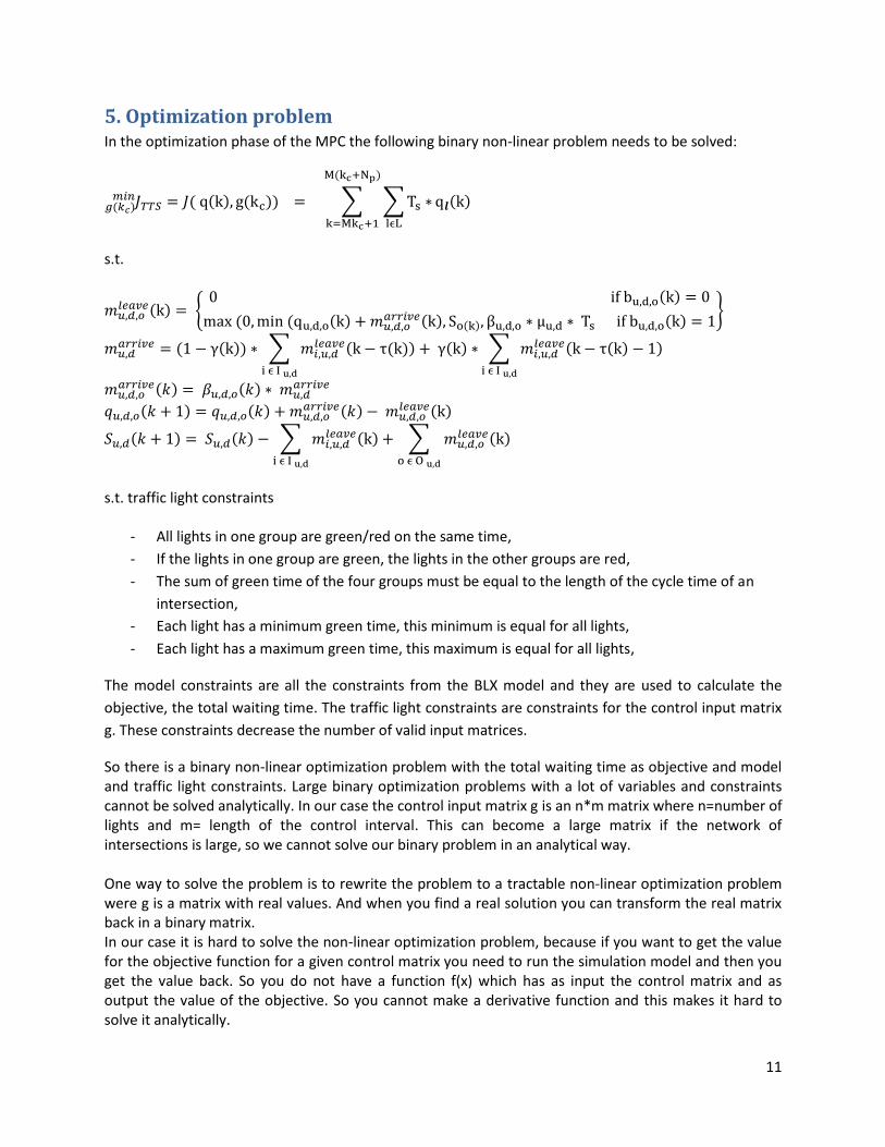
5. Optimization problem In the optimization phase of the MPC the following binary non-linear problem needs to be solved:

s.t.

s.t. traffic light constraints

- All lights in one group are green/red on the same time,

- If the lights in one group are green, the lights in the other groups are red,

- The sum of green time of the four groups must be equal to the length of the cycle time of an

intersection,

- Each light has a minimum green time, this minimum is equal for all lights,

- Each light has a maximum green time, this maximum is equal for all lights,

The model constraints are all the constraints from the BLX model and they are used to calculate the

objective, the total waiting time. The traffic light constraints are constraints for the control input matrix

g. These constraints decrease the number of valid input matrices.

So there is a binary non-linear optimization problem with the total waiting time as objective and model and traffic light constraints. Large binary optimization problems with a lot of variables and constraints cannot be solved analytically. In our case the control input matrix g is an n*m matrix where n=number of lights and m= length of the control interval. This can become a large matrix if the network of intersections is large, so we cannot solve our binary problem in an analytical way. One way to solve the problem is to rewrite the problem to a tractable non-linear optimization problem were g is a matrix with real values. And when you find a real solution you can transform the real matrix back in a binary matrix. In our case it is hard to solve the non-linear optimization problem, because if you want to get the value for the objective function for a given control matrix you need to run the simulation model and then you get the value back. So you do not have a function f(x) which has as input the control matrix and as output the value of the objective. So you cannot make a derivative function and this makes it hard to solve it analytically.

12

By the fact that we have constraints for the control input and constraints for a model that you need to use to calculate the objective it is not easy to find some numerical algorithms that solve the problem. So that is the reason a heuristics is developed to solve the optimization problem.

5.1 Heuristics

First some basic ideas for a heuristic approach were made, and some tests are made to check if this basic heuristics give some reasonable result. After that different changes were made in the heuristics and if these changes gave a better result they were saved. In the results section some of these test are shown and a there is a deeper description of how the heuristics were formed. The following heuristic approach is used:

- First determine in which order the traffic lights are green, this is done using the following method: At the start of each control interval for each order an initial matrix is made. This is a matrix where each group has a green time period of the length of a control interval divided by the number of groups. The begin time of the green period of a group depends on the order of the lights. For each order the total waiting time for the following control interval, using this matrix as control input is calculated. The order that has the lowest waiting time is chosen as order for the next interval.

- Given the specified order the lengths for all groups are decreased and increased to all possible lengths. If the length of group one is increased the length of the following group is decrease. Each time when a new matrix is made the simulation model is run with this matrix and the total waiting time is calculated. When the waiting time is lower than the current optimal value the matrix and the corresponding waiting time are stored as optimal values.

When the model is used for the first time for a given dataset the optimal values for different variables like, the minimum green time and the cycle time, should be calculated.

13

6. Traffic light control in Amsterdam In Amsterdam there are a lot of intersections that use traffic light control, and the control of these lights is done by the spatial planning service department of Amsterdam. The control of these traffic lights is a very complex problem, which is caused by the high number of different road users like cars, cyclists, pedestrians, trams, metros, and busses. These different road users also have different priorities, at the intersections in the centre of the city bikes and pedestrians have more priority then cars. And at intersections with a tram, bus or metro line, these have a higher priority than the other road users. So they cannot use the same control technique for all intersections; there are a lot of different optimization problems. This is the reason that in the most parts of Amsterdam isolated traffic light control are used, because if two intersections in a row have different priorities it is not optimal to solve this in a coordinated way. There are only a few networks of intersections were they use coordinated control; there are some green waves in the city for cars and bikes. And in Amsterdam-Southeast they are working on a coordinated control for a network of intersections. This is possible because there are not many other road users than cars. Most traffic light controllers use traffic -response algorithms, given the current traffic states a fixed planning is made for the next control interval, but the green time slots for the lights can be made longer or shorter if the controller measures that the number or cars is higher or lower than the expectations. During rush hours the insensitivity of cars is higher and then the cycle time of an intersection is longer. From the planning service department of Amsterdam a dataset with information of a green wave at the Wibautstraat in Amsterdam is received. This green wave is a route with thirteen intersections; for this paper only a network with four of these intersections is used. In figure 3 this route is presented.

Fig 3. Map of the green wave at the Wibautstraat

14

The dataset of this network includes the distance between the intersections, the arriving rates, the fraction of cars that turns left/right, the cycle times and the green time periods. The data is from a Tuesday in April 2012 between 14:00 and 15:00. In table one the most important data is shown.

Weesperplein Rijnspoorplein Ruyschstraat 1e oosterparkstraat

Cycle time 66 66 66 66

Arriving cars (city in)

900 840 940 1000

Arriving cars(city out)

950 1085 1000 985

Arriving cars (side roads)

100 300 50 50

Green time (city in)

25 24 29 28

Green time (city out)

23 19 25 26

Distance to next intersection

130 300 130 0

Table 1. Data of the intersections at the Wibautstraat

The given dataset is used for all tests in the results section.

15

7. Results In this section the results of different tests are presented, some tests are done to determine the best approach to find the order of the lights and to find the optimal values for different variables in the BLX model. For all tests we use the data from the green wave at the Wibautstraat in Amsterdam. There are four intersections; the cycle time of each intersection is 64 seconds. The minimum green time length is 5 seconds and the maximum green time length is 64-3*5= 49 seconds. The model is run over 20 control intervals each interval has a length of 64 seconds. When average values are calculated, the model is run fifty times (50*20=1000 control intervals).

7.1 Order of the lights

First we want to check what the influence of the order of the four groups is. When we have for example the order 2,3,4,1 then first the second group is green, then the third group is green etc. At the moment we assume that this order is the same for all intersections. The following two methods are used to determine the best order of the lights.

- At the start of each control interval for each order an initial matrix is made. This is a matrix where each group has a green time period of the length of a control interval divided by the number of groups. The begin time of the green period of a group depends on the order of the lights. For each order the total waiting time for the following control interval, using this matrix as control input is calculated. The order that has the lowest waiting time is chosen as order for the next interval.

- At the begin of each interval for each possible order the second part of the heuristic approach (increasing and decreasing of the green time periods) is used to calculate the best control input for the next control interval using that order. Then the order that gives the best result is chosen as order for the lights for the next interval.

To see if it is important to choose an order, a plot is made of the waiting time for one control interval for all twenty-four different orders using both methods.

Fig. 4 The total waiting time for two different order methods

16

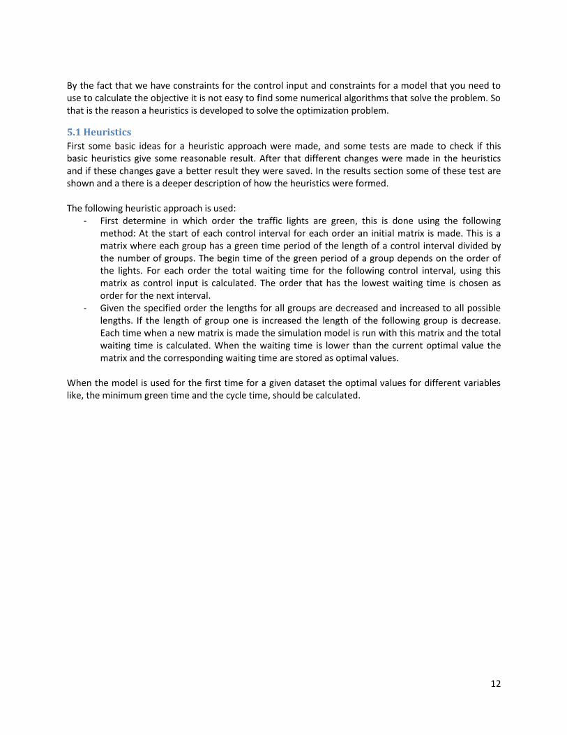
In figure four we see that the variation is high between the different orders. So the influence of the order of the groups is high and it is important to determine the best order. The lines of both methods have almost the same trend, so in most cases they should give the same outcome. The difference in calculation time is high between the two methods. When we run the model with twenty control intervals using the heuristic order method it takes more than two minutes, the model with the initial matrix order method takes a few seconds. To see what the overall performance of both methods is, the total waiting time over twenty control intervals is calculated for fifty runs. In figure five the results are shown:

Fig. 5 The average waiting time over 20 control intervals for 50 runs

In figure five we see that the results for both methods are lying in the same array, the average for the initial order method is 2104 and the average for the heuristic order method is 2187. The model is much faster when the initial order method is used and the results are almost the same as when the heuristic order method is used. So for the next tests the order of the traffic lights will be determined by using the initial order method.

7.2 Different cycle times

The cycle time of an intersection is the time that it takes before all traffic lights at that intersection had a green time period. We assume that the cycle time is the same for all intersections in the network and that the cycle time is the same for a specified period and does not change each control interval. To see what the influence of the cycle time is on the total waiting time the following test was performed: The model is run for different cycle times; the cycle times must be a multiple of four. Because the length of a control interval is equal to the cycle time, the number of control intervals is chosen such that the total simulation time lies around 1280 seconds. For each cycle time the model is performed fifty times, and the average total waiting time for the fifty runs is calculated. The simulation time is not the same for each cycle time, so these average values are scaled to the average value for 1280 seconds. The values are shown in the following graph.

17

Fig. 6 The total waiting time for different cycle times

From figure six we can see that a low cycle time gives high waiting times, this can be explained by the fact that the lights at links with a high arrival rate (the green wave) have smaller green time periods. When the cycle times are high the waiting time is also high, because the intersections are linked with each other and when the cycle times are high the intersections could not react fast on each other. The best cycle time for the intersections at the Wibautstraat is 60 seconds. For the next tests we assume a cycle time of 60 seconds instead of 64 seconds.

7.3 Boundaries

In the simulation model there is a maximum and a minimum value for the length of the green time period for each light. A cycle time of 60 seconds and a maximum time of 60-3*4= 48 seconds are used to calculate the average waiting time for different minimum values.

Fig 7. The total waiting time for different minimum lengths of the green time period

In figure seven we could see that the total waiting time is the lowest when the minimum length is one, this can be explained by the fact that in our dataset the side roads at the green wave have low arrival rates and it is optimal to put these lights on red and the lights with high arrival rates on green. But it is

18

not friendly to use this minimum length, because then it could be possible that some cars have to wait a long time. So then the best values should be four seconds, because then the waiting time is lower than we you use three or five as minimum. And in four seconds the few cars at the queue could leave. With a minimum green time length of four seconds the best maximum boundary is the largest possible green time length. This maximum value is 48 seconds (60-3*4).

7.4 Green Wave

The optimal values for the above variables are found and now the model is run with these values and the average lengths for all groups of lights and all intersections are calculated. These are shown in table two.

Group/Intersection Weesperplein Rijnspoorplein Ruyschstraat 1e oosterparkstraat

1 10 15 14 10

2 34 23 20 32

3 8 14 16 9

4 8 8 10 9 Table 2. The average green time lengths for all groups of lights and all intersections.

We see that the green time period of group two is the highest for each intersection. This is what we expected, because these are the lights that are lying on the green wave. At the intersection Rijnspoorplein the value for group two is lower in comparison with the order intersections; the reason for this is that the arrival rates for the other lights at this intersection are higher. At last the lengths of the green time period of group two of each intersection are compared with the green time periods given by the spatial planning service department of Amsterdam.

Intersection Simulation Model Real Values

Weesperplein 34 25

Rijnspoorplein 23 24

Ruyschstraat 20 29

1e oosterparkstraat 32 28 Table 3: Green time lengths given by the simulation model and the real values

In table three we see that the results of the simulation model are not exact the same as the green time

periods given by the spatial planning service department of Amsterdam. This can be declared by the fact

that the model that is used in practice also has to deal with other road users.

19

8. Conclusion and further research An answer is given to the main question, and a advice on further research is given Is the BLX model a reliable and fast model to use for Model Predictive Control? The BLX model is a fast model, but when you use an extensive approach in the optimization part it becomes slower. When you use the model in a real time situation is should be very fast to use it. So if you use the BLX model with a simple method to solve the optimization problem it is suitable to use, but when the model has to run a lot of times in the optimization part it is not fast enough. What is the influence of changing different input parameters of the model? For the heuristic approach two methods to determine the order of the lights are compared with each other; the simple and fast method give almost the same results as the extensive and slow method. And thus the simple method is used for the other test. The intersections at the Wibautstraat all have a cycle time of 66 seconds, to see if this is the optimal value the model is run with different cycle times. The graph with results has a u-shape with 60 seconds as minimum. When the cycle time is higher the lights at one intersection cannot react fast on the lights at other intersections and when the cycle time is lower the green time period of the green wave becomes lower. To be sure that all lights are green once during a cycle time a minimum green time length is set. The total waiting time is the lowest when there is a minimum of one and it grows when the minimum grows, but when the minimum is four the waiting time is lower then at two and five. A minimum of four is the best, but then the cars at the queue have not enough time to leave, so the optimal minimum time is then four seconds. Is the used heuristic approach a good way to solve the optimization problem? The results using the heuristic approach are compared with the real results and the results have the same pattern. They are not exact the same, but a reason for this could be the fact that the methods used in practice also have to deal with other road user. The heuristic approach does not give the globally optimal solution but it gives a good local solution. Further research can be done on other prediction models, are there better and faster models than the BLX model? An other important question is how to solve the optimization problem, can the problem be rewritten in such a way it is easy to solve?

20

9. References

1: Haijema, R. (2008), “Solving large structured Markov Decision Problems for perishable inventory management and traffic control”. 2: Lin, S. and Schutter, B. de and Xi, Y. and Hellendoorn, H. (2009), “Study on fast model predictive controllers for large urban traffic networks”, Proceedings of the 12th International IEEE conference on Intelligent Transportations Systems (ITCS 2009), St. Louis, Missouri, pp. 691-696. 3: Papageorgiou, M. and Diakaki, C. and Dinopoulou, V. and Kotsialos, A. and Wang, Y. (2003), “Review of road traffic control strategies”, Proceedings of the IEEE, 91 (12). pp. 2043-2067. 4: Tettamanti, T. And Varga, I. (2009),“Distributed traffic control system based on model predictive control”, Periodica polytechnic.