simulation of the heat exchangers dynamics in...

Simulation of the Heat Exchangers Dynamics in MATLAB&Simulink

PAVEL NEVRIVA, STEPAN OZANA, LADISLAV VILIMEC Department of Measurement and Control, Department of Energy Engineering

VŠB-Technical University of Ostrava 17. listopadu 15/2172, Ostrava-Poruba, 708 33

CZECH REPUBLIC [email protected] http://kat455.vsb.cz

Abstract: - Heat exchangers that transfer energy from flue gas to steam are important units of thermal power stations. Their inertias are often decisive for the design of the steam temperature control system. In this paper, the analysis and the simulation of the dynamics of the steam superheater are discussed. Superheater is simulated as a unit of a control loop that generates steam of desired state values. To simulate the steam superheater on the computer, the exchanger is described by the set of partial differential equations. The equations are then solved numerically by modified finite difference method. Discussion of method and qualitative and quantitative results are presented. Paper describes use of Simulink S-functions which make it possible to set-up the most complex systems with complicated dynamics. There’s a comparison of M and C S-functions, which are two main approaches when building user-defined blocks in Simulink, regarding both the performance and the efficiency of the simulation for M and C versions of the codes and the possibility to perform a real-time simulation. Key-Words: - Simulation, Heat exchangers, Superheaters, Partial differential equations, Finite difference method, MATLAB&Simulink, S-functions, Real-time

1 Introduction Heat exchangers convert energy from a heating medium to a heated medium. In this paper, the steam superheater is the heat exchanger that transfers energy from flue gas to steam in the boiler of a thermal power station or a heating plant. The heating medium is usually the flue gas generated by combustion of some kind of fuel. The heated medium is usually steam or the mixture of steam and air. Fig.1 presents the example of an arrangement of superheaters and reheaters in a big boiler. In this paper, the analysis and the simulation of the dynamics of thermal state variables of a superheater are discussed. Superheater is considered to be the part of the control loop that generates steam of desired state values. Note that there are many types and configurations of superheaters. Moreover, one energy block of a power station usually contains several different superheaters. The interconnections of superheaters differ from case to case. The mathematical model of the superheaters has to be therefore universal. It has to accommodate different types of heat exchanging units and has to interface models of piping, valves, controllers, and other parts of the control system. The numerical method applied to construction of numerical models of superheaters should be also suitable for numerical simulation of those very heterogeneous parts of a boiler. Technical designs of the superheaters result in constructions that are complicated and complex. Accuracy of a three-dimensional dynamical model of a superheater is limited by the accuracy of its parameters.

To simulate the dynamics of the superheater, the one-dimensional model of the superheater was developed and tested. The following paragraphs deal with superheaters that operate in a normal operating mode.

Fig.1 The example of an arrangement of superheaters and reheaters in a big boiler, [7]

WSEAS TRANSACTIONS on SYSTEMS and CONTROL Pavel Nevriva, Stepan Ozana, Ladislav Vilimec

ISSN: 1991-8763 519 Issue 10, Volume 4, October 2009

3 The role of superheaters The thermal power station transfers thermal energy into electrical one. The physical model of operation of steam heat engine of a common power plant can be simulated by the Rankine cycle. The Rankine cycle is sometimes referred to as a practical Carnot cycle. The main difference is that a pump is used to pressurize liquid instead of compressing gas. The expansion of steam is expected here through a turbine. The ideal Rankine cycle when acting as a heat engine consists of the four steps:

• Process 1-2: Isentropic pressurizing of the working saturated liquid (water) from low to high pressure.

• Process 2-3: Isobaric heating of the high pressure liquid at a boiler by a heat source (flue gas) to become a dry saturated vapor.

• Process 3-4: Isentropic expansion of the dry saturated vapor through a turbine, generating power. Some condensation may occur.

• Process 4-1: Isobaric isothermal cooling the wet vapor at a condenser to become a saturated liquid.

In an ideal Rankine cycle, the processes 1-2 and 3-4 are isentropic represented by vertical lines on the Ts diagram. In real Rankine cycle, adiabatic models of pump and turbine are more physical. See Fig. 1., where T stands for temperature and s for entropy. There is also a small pressure drop at the point 3'.

Fig.1 Rankine cycle with superheating The Rankine cycle 1-2-3-4 prevents the vapor ending up in the superheat region after the expansion in the turbine, which reduces the energy removed by the condensers but as the water condensates, water droplets

hit the turbine blades, decreasing the life of turbine blades and efficiency of the turbine . To increase the efficiency η of the thermomechanical cycle and to limit the droplet formation, in thermal power stations the saturated steam is superheated in superheaters. By superheating the steam, state 3 moves to the right of the diagram (3'). Efficiency of the cycle is increasing, inout QQ−=η 1 ,

where inQ is heat in and in outQ is heat out.

Throughout the expansion (3'- 4'), the water droplets do not occur inside the turbine. Many modifications of this principal idea are used in modern steam turbines.

2 Mathematical model of a superheater In the basic form, the thermal model of a superheater is defined by seven state variables. They are as follows:

( )txT ,1 temperature of steam

( )txT ,2 temperature of flue gas

( )txTS , temperature of the wall of the heat

exchanging surface of the superheater ( )txp ,1 pressure of steam

( )txp ,2 pressure of flue gas

( )txu ,1 velocity of steam

( )txu ,2 velocity of flue gas where x is the space variable along the active length of the wall of the heat exchanging surface of the superheater and t is time. Fig.2 shows the principal schema of the physical state variables at a counterflow steam superheater.

Fig.2 Principal schema of the physical state variables at a counterflow steam superheater. In the model, presented in this paper, both the pressure and the flow velocity of the flue gas are assumed to be



the given functions independent of length. That is the pressure ( ) ( )tptxp 22 , = acts usually as the input and

velocity ( ) ( )tutxu 22 , = is the function of ( )tp2 . Three of the five remaining state variables are selected to be the input and output variables, and the two are the superheater’s state variables. Input and output variables are usually temperature of steam ( )txT ,1 , temperature of

flue gas ( )txT ,2 , and pressure of steam ( )txp ,1 . Superheater’s state variables are velocity of the steam

( )txu ,1 and temperature of the wall of the heat exchanging surface of the superheater, temperature of the wall, ( )txTS , .

Applying the energy equations, Newton’s equation, and heat transfer equation, and principle of continuity the behavior of five state variables of superheater can be well described by five nonlinear partial differential equations, PDE, as follows: Reduced energy equation for flue gas:

( ) 0α

ρ

222

222

222 =−+⎥⎦

⎤⎢⎣

⎡

∂∂+

∂∂

SS

TTt

T

x

Tu

O

Fc (1)

Heat transfer equation describes the transfer of heat from burned gases to steam via the wall:

0

αα 22

2

11

1 =−−−−∂

∂

O

GcTT

O

GcTT

t

T

S

SS

S

SSS (2)

Principle of continuity for steam:

0

1

11

1

11

1

11

1

1

11

1

1

1

111

1

1

11

1

11

1

=∂∂+

⎪⎭

⎪⎬⎫⎟⎟⎠

⎞⎜⎜⎝

⎛

∂∂

∂ρ∂+

∂∂

∂ρ∂+⎟⎟

⎠

⎞⎜⎜⎝

⎛

∂∂

∂∂+

∂∂

∂∂ρ+

⎪⎩

⎪⎨⎧

⎟⎟⎠

⎞⎜⎜⎝

⎛

∂∂

∂∂+

∂∂

∂∂ρ+⎟⎟

⎠

⎞⎜⎜⎝

⎛

∂∂

∂ρ∂+

∂∂

∂ρ∂

ρ

x

u

t

T

Tt

p

pF

t

T

T

F

t

p

p

F

x

T

T

F

x

p

p

Fu

x

T

Tx

p

pFu

F

(3)

Newton’s partial differential equation for steam:

( )0

sin

1111

11

11

111

=λρ+

θρ+∂

∂ρ+

∂∂

ρ+∂

∂

uu

gt

u

x

uu

x

p (4)

Energy partial equation for steam:

{ } { } ( ) 01

....

22

1111111

21

1111

21

111

=−α−∂∂+

∂∂+

⎪⎭

⎪⎬⎫

⎪⎩

⎪⎨⎧

⎟⎟

⎠

⎞

⎜⎜

⎝

⎛+ρ

∂∂+

⎪⎭

⎪⎬⎫

⎪⎩

⎪⎨⎧

⎟⎟

⎠

⎞

⎜⎜

⎝

⎛+ρ

∂∂

FTTOzgup

xup

x

uTcu

x

uTc

t

SS

(5)

( )Tpcc ,11 = heat capacity of steam at constant pressure

J.kg-1

K-1

( )Tpcc ,22 = heat capacity of flue gas at constant pressure

J.kg-1

K-1

Sc heat capacity of superheater’s wall material

J.kg-1

K-1

( )xFF 11 = steam pass crossection m2

( )xFF 22 = flue gas channel crossection

m2

g acceleration of gravity m.s-2

( )xGG = weight of wall per unit of length in x direction

kg.m-1

L active length of the wall m ( )xOO 11 = surface of wall per unit of

length in x direction for steam

m

( )xOO 22 = surface of wall per unit of length in x direction for steam

m

( )txpp ,11 = pressure of steam Pa

( )txpp ,22 = pressure of flue gas Pa

t time s ( )txTT ,11 = temperature of steam ºC

( )txTT ,22 = temperature of flue gas ºC

( )txTT SS ,= temperature of the wall ºC

( )txuu ,11 = velocity of the steam in x direction

m.s-1

( )txuu ,22 = velocity of the steam in x direction

m.s-1

x space variable along the active length of the wall

m

( )xzz = ground elevation of the superheater

m

1Sα heat transfer coefficient between the wall and steam

J.m-2

s-1

K-1

2Sα heat transfer coefficient between the wall and flue gas

J.m-2

s-1

K-1

( )x1λ steam friction coefficient 1

θ superheater’s constructional gradient

1

( )Tp,11 ρ=ρ density of steam kg.m-3

( )Tp,22 ρ=ρ density of flue gas kg.m-3

3 Numerical method The set of PDE (1)-(5) can be solved by many methods. Equations (1)-(5) have two independent variables. They are space variable length [ ]Lx ,0∈ and time [ )∞∈ ,0t .



It follows that PDE (1)-(5) are not suitable for solution by finite elements method. Here, the finite difference method was used. The method was modified to facilitate the simulation of control problems. The modification can be demonstrated as follows: Let PDF (6) is given.

( ) ( ) ( ) ( ) ( )[ ] [ )∞∈∈

=∂

∂+∂

∂

,0,,0

,,

,,

,

tLx

txCt

txytxB

x

txytxA (6)

where

( )( ) ( ) ( ) functionsknownare,,,,,

variablephysicalany is

txCtxBtxA

x,ty

PDF (6) is to be solved by the modified finite difference method. The interval L of the space coordinate x is divided into

1−� intervals of discretization of x . Intervals are of

constant length 1−

=�

Lh .

The derivatives ( )x

txy

∂∂ ,

of ( )txy , are in the grid points

�,,2,1, �=ixi , approximated by the differences of

the second order as follows:

( ) ( ) ( )

( ) ( ) ( )

( ) ( ) ( )

( ) ( ) ( )�

�

Dh

tytyy

x

txy

Dh

tyty

x

txy

Dh

tyty

x

txy

Dh

tytyy

x

txy

nnn

xx

xx

xx

xx

=+−

≈∂

∂

=−

≈∂

∂

=−

≈∂

∂

=−+−

≈∂

∂

−−

=

=

=

=

2

34,

2

,

2

,

2

43,

12

324

213

1321

3

2

1

�

(7)

where

( ) ( ) �,,2,1,, �== = itxytyixxi

The derivatives ( )

t

txy

∂∂ ,

of ( )txy , in grid points

�,,2,1, �=ixi can be assigned as

( ) ( )

�,,2,1,,

�=≈∂

=i

dt

tdy

dt

txy i

xx i

(8)

The PDE is approximated by the set of � ordinary differential equations, ODE. The independent variable of ODE is time.

( ) ( ) ( ) ( ) �,,2,1,,,, �==∂

∂+ itxC

t

tytxBDtxA i

iiii (9)

Integration of the set of ODE by some standard numerical method, Euler method, Runge-Kutta methods, linear multistep methods, or any other numerical formula can be applied. The order of the model may be rather large. Let us neglect the complex model of boiler and turbine and consider only its part consisting of four heat exchangers and five interconnecting steam lines. Representing the length coordinate of every exchanger and every interconnecting steam line at twenty nods, we obtain (4+5)*5*20=900 ODE of the first order. Adaptation of the method covers the advantages of the standard finite element method and is applicable to simulation of the complex superheater control problems, where the integration in time is frequent. Dynamics of superheater’s state variables is unequal. The change of the input pressure of steam ( )tp ,01 propagates through the superheater’s tract with velocity of the sound. Velocity of both, the steam and the flue gas is up to ten meters per second. On the other hand, the time inertia of the steam output temperature with respect to the change of the flue gas input temperature may be measured in tens of minutes. It results in small integration step of numerical method used for integration of the system of ODE. As for the computation time, numerical methods for the stiff equations have certain advantage over the standard methods. In example presented below, the MATLAB Stiff/NDF formula was used. Sometimes, in operating point, the derivatives of parameters of in PDE (3) can be neglected. Then, also the flow velocity and the pressure of steam can be assumed to be the known functions of time. Under these presumptions, the mathematical model of superheater describes only the relatively slow heat transfer between media. For constant steam pass crossection ( ) 11 FxF = steam velocity and steam pressure act as known inputs independent of length x ,

( ) ( )tutxu 11 , = , ( ) ( )tptxp 11 , = . For horizontal wall the equations (1)-(5) are replaced by equations (10)-(12):



Reduced energy equation for flue gas:

( ) 0222

222

222 =−+⎥⎦

⎤⎢⎣

⎡

∂∂+

∂∂

αρ

SS

TTt

T

x

Tu

O

Fc (10)

Heat transfer equation of the wall:

0

22

2

11

1 =

α

−−

α

−−

∂∂

O

GcTT

O

GcTT

t

T

S

S

S

S

S

SS (11)

Reduced energy equation for steam:

( ) 0111

111

111 =−+⎥⎦

⎤⎢⎣

⎡

∂∂+

∂∂

αρ

STTt

T

x

Tu

O

Fc (12)

4 Example The dynamics of the superheater of the medium-size experimental steam generator was simulated. The superheater is of a counter-flow arrangement. At time −= 0t the superheater is at its steady-state. Temperatures of the steam, flue gas, and the wall are stabilized. It follows that pressure of the steam and flue gas is stabilized too. The steady state of the superheater is defined by PDE (1)-(5) for actual parameters of the superheater and actual parameters of both heat transferring media at the inputs to the superheater. Exact description of all parameters of the superheater is beyond the extent of this paper. Typical parameters of the selected superheater are as follows: active length of the wall 60≈L m, weight of wall per unit of length in x

direction 1kg.m350 −≈G .

Steam velocity 11 m.s11 −≈u .Flue gas velocity

12 m.s7 −−≈u .

Such superheater represents an unit of an extremely great thermal inertia. Steam input temperature

( ) C950,01�=T . Flue gas input temperature

( ) C4600,2�=LT .

The finite difference method approximates the PDE (1)-(5) by 100205 =× nonlinear ODE of the first order. Calculating the steady state of the superheater, 100 steady-states of its numerical approximation were found.

Note that in presented example, the steady-state steam

output temperature ( ) C4410,1�=LT , steady state flue

gas output temperature ( ) C1750,02�=T . Solution of

PDE (1)-(5) is usually made by method of simulation, parameters of superheater are optimized with respect to technology. To study the dynamics of the superheater, two simulation experimens are presented below.

4.1 Step change of steam At time 0=t , there is the step change of parameters of the steam at the input to the superheater. The temperature of the input steam is increased by the step

value ( ) 0C10,0Δ 1 ≥+= ttT � .

Change of one state variable results in changes of all remaining state variables. Fig.3 shows the temperature increase ( )tLT ,Δ 1 of the steam at the output and the

temperature increase ( )tT ,0Δ 2 of the flue gas at the output.

Fig.3 Increase of temperatures of media at the outputs of the superheater as the response to the step

increase ( ) 0C10,0Δ 1 ≥+= ttT � of the temperature of

the steam at the input. ( )tLT ,1Δ is increase of the temperature of the steam

at the output, ( )tT ,02Δ is increase of the temperature of the flue gas

at the output Fig.4 shows, in logarithmic scale, the temperature wave

( )txT ,1 in the beginning of the process.



Fig.4 Increase of temperature ( )txT ,Δ 1 of steam in the superheater as the response to the step increase

( ) 0C10,0Δ 1 ≥+= ttT � of the temperature of the steam

at the input. 4.2 Step change of flue gas At time 0=t , there is the step change of parameters of the flue gas at the input to the superheater. The temperature of the input flue gas is increased by the step

value ( ) 0C10,Δ 2 ≥+= ttLT � . Fig.5 corresponds to

Fig.3. It shows the temperature increase ( )tLT ,Δ 1 of the steam at the output and the temperature increase

( )tT ,0Δ 2 of the flue gas at the output.

Fig.5 Increase of temperatures of media at the outputs of the superheater as the response to the step

increase ( ) 0C10,Δ 2 ≥+= ttLT � of the temperature of

the flue gas at the input. ( )tLT ,1Δ is increase of the temperature of the steam

at the output, ( )tT ,02Δ is increase of the temperature of the flue gas

at the output.

Fig.6 shows, in logarithmic scale, the temperature wave

( )txT ,2 in the beginning of the process.

Fig.6 Increase of temperature ( )txT ,2 of flue gas in the superheater as the response to the step increase

( ) 0C10,Δ 2 ≥+= ttLT � of the temperature of the flue

gas at the input.

5 Simulation Software for Concurrent and Counter-flow Heat Exchangers The paragraph 5 presents the problems of construction of the simulation software used for the simulation of the superheaters dynamics in MATLAB&Simulink. It is demonstrated the difference between the codes for those two types of heat exchangers. In the Paragraph 5, the theme is illustrated on the simplified model of the superheater, see equations (10)-(12).

5.1 Simplified Mathematical Model of the Supertheater Simplified mathematical model of the superheater is given by a set of equations (10)-(12) which can be transformed to the form (13)-(15)

⎥⎦

⎤⎢⎣

⎡

∂∂+

∂∂=−

t

T

x

TuTTS

11111 τ ( (13)

⎥⎦

⎤⎢⎣

⎡

∂∂+

∂∂=−

t

T

x

TuTTS

22222 τ (14)

t

TTTTT S

S

S

S

S∂

∂=−+−

2

2

1

1ττ

(15)

where Sτandτ,τ 21 are time constants of the

system. For purposes of applying finite difference method by means of Simulink S-functions, particular partial derivatives of state variables must be expressed as follows:



( )x

TuTT

t

TS ∂

∂−−=∂

∂ 111

1

1τ

1 (16)

( )x

TuTT

t

TS ∂

∂−−=∂

∂ 222

2

2τ

1 (17)

( ) ( )SS

SS

S TTTTt

T −+−=∂

∂2

21

1 τ

1τ

1 (18)

5.2 Software Solution of the Simplified Model in Simulink S-functions (system-functions) provide a powerful mechanism for extending the capabilities of Simulink. This paragraph describes what S-function is and when and why it is convenient to use one. S-functions make it possible to add customized algorithms to Simulink models, either written in MATLAB or C. By following a set of simple rules it possible to implement the algorithms in an S-function. After S-function has been written and placed its name in an S-Function block (available in the User-defined Functions sublibrary), it’s time to customize the user interface by using masking. An S-function is a computer language description of a dynamic system. S-functions can be written using MATLAB or C. C language S-functions are compiled as MEX-files using the mex utility described in the Application Program Interface Guide. As with otherMEX-files, they are dynamically linked into MATLAB when needed. S-functions use a special calling syntax that enables you to interact with Simulink’s equation solvers. This interaction is very similar to the interaction that takes place between the solvers and built-in Simulink blocks. The form of an S-function is very general and can accommodate continuous, discrete, and hybrid systems. As a result, nearly all Simulink models can be described as S-functions. The most common use of S-functions is to create custom Simulink blocks. S-functions can be effectively used for a variety of applications, including: •Adding new general purpose blocks to Simulink •Incorporating existing C code into a simulation •Describing a system as a mathematical set of equations •Using graphical animations An advantage of using S-functions is that it is possible to build a general purpose block that can be used many times in a model, varying parameters with each instance of the block, as it can be seen on Fig.7.

Fig.7 Principal scheme of simulation in Simulink An M-file or a CMEX-file that defines an S-Function block must provide information about the model; Simulink needs this information during simulation. As the simulation proceeds, Simulink, the ODE solver, and the M-file interact to perform specific tasks. These tasks include defining initial conditions and block characteristics, and computing derivatives, discrete states, and outputs. Simulink provides a template M-file S-function that includes statements that define necessary functions, as well as comments to help with writing the code needed for a particular S-function block. M-file S-functions work by making a sequence of calls to S-function routines, which are M-code functions that perform tasks required by customized S-function. This table lists the S-function routines available to M-file S-functions. C MEX-file S-functions have the same structure and perform the same functions as M-file S-functions. In addition, C MEX S-functions provides more functionality than M-file S-functions.The physical interpretation of simplified model of both concurrent and counter-flow superheater demonstrated on Fig.8 and Fig.9, where ( )txT ,1 is the temperature of steam,

( )txT ,2 is the temperature of flue gas and ( )txTS , is

the temperature of the sperheater’s heat exchanging surface, i.e. superheater’s wall.



T (0,t)1 STEAMT (x,t)1

T (0,t)S T (x,t)S T (L,t)S

T (0,t)2

T (L,t)1

FLUE GAST (x,t)2 T (L,t)2

Lx0

WALL

Fig.8 Simplified model. Physical state variables of a concurrent superheater

T (0,t)1 STEAMT (x,t)1

T (0,t)S T (x,t)S T (L,t)S

T (0,t)2

T (L,t)1

FLUE GAST (x,t)2 T (L,t)2

Lx0

WALL

Fig.9 Simplified model. Physical state variables of a counter-flow superheater For a concurrent heat exchanger, the main goal of this task is to determine temperatures of a steam and a flue gas ( )tLT ,1 and ( )tLT ,2 as reactions on inlet

temperatures ( )tT ,01 and ( )tT ,02 . As for a counter-

flow heat exchanger, it is determination of temperatures of a steam and a flue gas ( )tLT ,1 and ( )tT ,02 as

reactions on temperatures ( )tT ,01 and ( )tLT ,2 .

5.3 Concurrent Heat Exchanger This paragraph describes use of finite difference method applied on a concurrent heat exchanger in detail, assuming C version of S-function. The principle of method see Paragraph 3 of this paper. The length L is divided into �+1 equidistant slices (nods) along x-axis according the scheme on Fig.10.

T1in

T2in

TS

x[0]

n = 0

x[N]

n = N

x[2N]

n = 2N

x[1]

x[N+1]

x[2N+1]

x[N-1]

n = N-1

x[2N-1]

n = 2N-1

x[3N-1]

n = 3N-1

x[N-2]

x[2N-2]

x[3N-2]

x[N-3]

x[2N-3]

x[3N-3]

T1out

T2out

Tsout

INLET SLICE 1 SLICE 2 SLICE N-1SLICE N(OUTLET)

T (0,t)1 T1(L, )t

T2(L, )tT (0,t)2

L0

h=L/N

...

...

...

Fig.10 Simplified model. Concurrent superheater. Notation of finite differences for state variables Notice: All of the following equations are stated for C S-functions, the first index starts from zero. For M version, the syntax is a bit different, round brackets are used for indexes and the first index starts with one. In accordance

with Fig.10, the following Simulink variables are introduced for state variables, their derivatives and outputs:

[ ] [ ] [ ] [ ][ ] [ ] [ ] [ ][ ] [ ] [ ] [ ]13,23,,12,2:

12,22,,1,:1,2,,1,0:

2

1

−−+−−+

−−

��

��

��

�

�

�

STTT

[ ] [ ] [ ] [ ]

[ ] [ ] [ ] [ ]

[ ] [ ] [ ] [ ]13,23,,12,2

12,22,,1,

1,2,,1,0

:

:

:

2

1

−−+

−−+

−−

��

��

��

�

�

�

dt

dt

dt

SdT

dT

dT

[ ][ ]12

1

2

1−≡

−≡��

��

out

outTT

Applying formulas (7) on a set of equations (16)-(17), the derivatives of the new discrete state variables can be approximated as follows: SLICE 1 (n = 0):

[ ] [ ] [ ]( ) [ ]h

Tux in

2

102

10 1

11

−−−

τ=

��

[ ] [ ] [ ]( ) [ ]h

Tu in

2

12

1 22

2

−+−−

τ=

��

[ ] [ ] [ ]( ) [ ] [ ]( )�� 21

201

221

−τ

+−τ

=SS

x

Due to the formula (7), the first and the last slice must be treated separately. For inner slices, there is a loop containing the formulas as follows: SLICES 2 to �– 1 (for n = 1 to �– 2):

[ ] [ ] [ ]( )[ ] [ ]

h

nnu

nnn

2

11

21

1

1−−+−

−+τ

=

��

��

[ ] [ ] [ ]( )[ ] [ ]

h

nnu

nnn

2

21

21

2

2��

��

+−++−

−+−+τ

=+

[ ] [ ] [ ]( )

[ ] [ ]( )��

��

21

21

2

2

1

+−τ

+

++−τ

=+

n

nnn

S

S



SLICE � (outlet, n = � – 1):

[ ] [ ] [ ]( )[ ] [ ] [ ]

hu

2

13243

1131

1

1

1−+−−−−

−−−−τ

=−

��

��

[ ] [ ] [ ]( )[ ] [ ] [ ]

hu

2

12322432

12131

12

2

2−+−−−−

−−−−τ

=−

��

��

[ ] [ ] [ ]( )

[ ] [ ]( )13121

1311

13

2

1

−−−τ

+

+−−−τ

=−

��

��

S

S

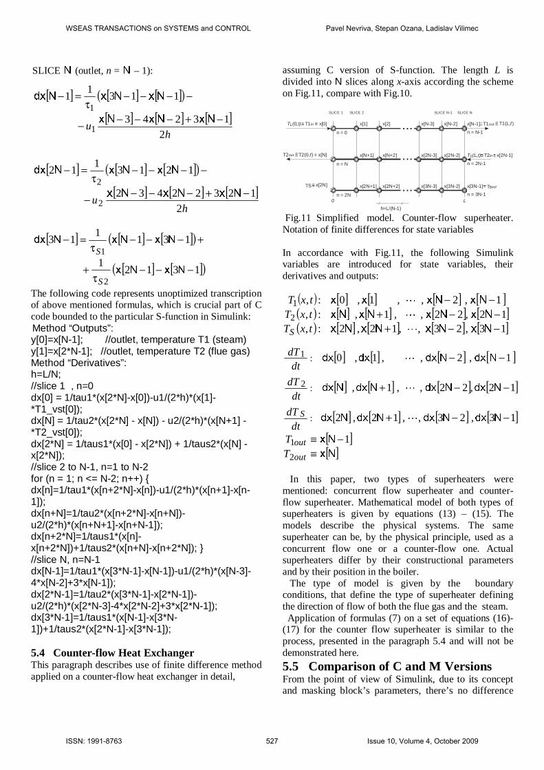
The following code represents unoptimized transcription of above mentioned formulas, which is crucial part of C code bounded to the particular S-function in Simulink: Method “Outputs”: y[0]=x[N-1]; //outlet, temperature T1 (steam) y[1]=x[2*N-1]; //outlet, temperature T2 (flue gas) Method “Derivatives”: h=L/N; //slice 1 , n=0 dx[0] = 1/tau1*(x[2*N]-x[0])-u1/(2*h)*(x[1]-*T1_vst[0]); dx[N] = 1/tau2*(x[2*N] - x[N]) - u2/(2*h)*(x[N+1] - *T2_vst[0]); dx[2*N] = 1/taus1*(x[0] - x[2*N]) + 1/taus2*(x[N] - x[2*N]); //slice 2 to N-1, n=1 to N-2 for (n = 1; n <= N-2; n++) { dx[n]=1/tau1*(x[n+2*N]-x[n])-u1/(2*h)*(x[n+1]-x[n-1]); dx[n+N]=1/tau2*(x[n+2*N]-x[n+N])-u2/(2*h)*(x[n+N+1]-x[n+N-1]); dx[n+2*N]=1/taus1*(x[n]-x[n+2*N])+1/taus2*(x[n+N]-x[n+2*N]); } //slice N, n=N-1 dx[N-1]=1/tau1*(x[3*N-1]-x[N-1])-u1/(2*h)*(x[N-3]-4*x[N-2]+3*x[N-1]); dx[2*N-1]=1/tau2*(x[3*N-1]-x[2*N-1])-u2/(2*h)*(x[2*N-3]-4*x[2*N-2]+3*x[2*N-1]); dx[3*N-1]=1/taus1*(x[N-1]-x[3*N-1])+1/taus2*(x[2*N-1]-x[3*N-1]); 5.4 Counter-flow Heat Exchanger This paragraph describes use of finite difference method applied on a counter-flow heat exchanger in detail,

assuming C version of S-function. The length L is divided into N slices along x-axis according the scheme on Fig.11, compare with Fig.10.

n = 0

n = N

n = 2N

x[1]

x[N+1]

x[2N+1]

x[2]

x[N+2]

x[2N+2]

x[N-1]

n = N-1

x[2N-1]

n = 2N-1

x[3N-1]

n = 3N-1

x[N-2]

x[2N-2]

x[3N-2]

x[N-3]

x[2N-3]

x[3N-3]

T1out

Tsout

SLICE 1 SLICE 2 SLICE N-1 SLICE N

T1(L, )t

L0

h (=L/ N-1)

T2inT (L,t)2x[N]T2out T2(0, )t

x[0]T1inT (0,t)1

TS x[2N]

...

...

...

Fig.11 Simplified model. Counter-flow superheater. Notation of finite differences for state variables In accordance with Fig.11, the following Simulink variables are introduced for state variables, their derivatives and outputs:

( ) [ ] [ ] [ ] [ ]( ) [ ] [ ] [ ] [ ]( ) [ ] [ ] [ ] [ ]13,23,,12,2:,

12,22,,1,:,1,2,,1,0:,

2

1

−−+−−+

−−

��

��

��

�

�

�

txTtxTtxT

S

[ ] [ ] [ ] [ ]

[ ] [ ] [ ] [ ]

[ ] [ ] [ ] [ ]13,23,,12,2

12,22,,1,

1,2,,1,0

:

:2

:1

−−+

−−+

−−

��

��

��

�

�

�

dtdT

dtdT

dtdT

S

[ ][ ]��

≡−≡

out

outTT

2

1 1

In this paper, two types of superheaters were mentioned: concurrent flow superheater and counter-flow superheater. Mathematical model of both types of superheaters is given by equations (13) – (15). The models describe the physical systems. The same superheater can be, by the physical principle, used as a concurrent flow one or a counter-flow one. Actual superheaters differ by their constructional parameters and by their position in the boiler. The type of model is given by the boundary conditions, that define the type of superheater defining the direction of flow of both the flue gas and the steam. Application of formulas (7) on a set of equations (16)-(17) for the counter flow superheater is similar to the process, presented in the paragraph 5.4 and will not be demonstrated here.

5.5 Comparison of C and M Versions From the point of view of Simulink, due to its concept and masking block’s parameters, there’s no difference



between working with C and M version of an S-function because the blocks behaves the same, as it is demonstrated on Fig.12.

TP6TP5TP4

TP3TP2TP1

800

T2_in2

800

T2_in1

200

T1_in2

200

T1_in1

Scope2

Scope1

superheaterC superheaterC superheaterC

superheaterM superheaterM superheaterM

Fig.12 Simulink scheme of M and C versions of S-functions, three heat exchangers set up in series The syntax of the codes inside the blocks is different. Generally, M structure of S-function has syntax of MATLAB language and the abilities are limited. C structure requires a bit of C programming but the performance and effectiveness are uncomparably higher. The comparison was done for simulation of 10 seconds for M and C version, depending on number of blocks in series and number of slices. Particular simulations are also compared to real time. Fig. 13 and Fig. 14 show the ratio MC tt vs. both the

number N of slices and the number B of blocks in series. Ct stands for time established for simulation in C

code Mt stands for time needed to perform the M code.

10 20 30 40 50 60 70 80 90 1000

1000

2000

3000

4000Tfinal=10

Number N of slices

t Mt C

/

B=3

B=6

B=12

B=24B=48

B=96

Fig.13 C and M S-functions time ratio vs. number of slices

0 10 20 30 40 50 60 70 80 90 1000

1000

2000

3000

4000Tfinal=10s

Number B of blocks

N=10

N=20

N=50

N=100

t Mt C

/

Fig.14 C and M S-functions time ratio vs. number of blocks in series Fig. 15 then describes the time needed for simulation of C code vs. real time. It states that even for a large

number of blocks in series and a large number of slices (B=96, N=100) the simulation is still 6 times faster than real time. On the other hand, Fig. 16 shows that M S-functions are inconvenient to use for systems with so complicated dynamics and it’s impossible to perform a real time simulation because even for a small number of slices and blocks in series (N=3, B=10) the simulation is much slower than real time.

10 20 30 40 50 60 70 80 90 1000

10

20

30

40

50

60

Number N of slices

t rt C

/

B=3

B=6

B=12

B=24

B=48B=96

Fig.15 Performance of C S-functions vs. real time

10 20 30 40 50 60 70 80 90 1000

0.2

0.4

0.6

0.8

Number N of slices

B=3B=6B=12

t rt M

/

Fig.16 Performance of M S-functions vs. real time 6 Performing Real-time Simulation There are some approaches how to implement the designed models on a specific hardware. It might be useful in some special cases, for example for adaptive control scheme with reference model, while the real data from the process can be measured, evaluated and performed on a hardware. It can also be used to control the process, provided the hardware is robust enough to be used in industry, for example IPC DAS controllers mentioned below. Generally as for real-time control, commonly used tools are Real Time Toolbox, Real Time Windows Target and xPC Target. They all include libraries with I/O blocks to access the hardware devices but they differ in concepts. The lowest programming level is offered by xPC Target which doesn't need any other operating system, only its own real time kernel. Generally, C-code for given platforms is generated by Real Time Workshop. xPC Target offers possibility to handle the model by communication cable (TCP/IP) by a host computer or by the LAN, using web explorer and any computer connected to the network. Web page is generated automatically, the needed sole is the Simulink scheme.



The main advantage of xPC Target is that the control scheme can stay absolutely the same and can be converted directly to the form executable on the hardware. On the other hand, this solution is very expensive due to licensing conditions. Besides PC/embedded PC platform with PC Target, it is also possible to use compact controllers. A programmable automation controller (PAC) is a compact controller that combines the features and capabilities of a PC-based control system with that of a typical programmable logic controller (PLC). A PAC thus provides not only the reliability of a PLC, but also the task flexibility and computing power of a PC. PACs are most often used in industrial settings for process control, data acquisition, remote equipment monitoring, machine vision, and motion control. Additionally, because they function and communicate over popular network interface protocols like TCP/IP, OLE for process control (OPC) and SMTP. As a typical PAC producer, ICP DAS will be mentioned, particularly its WinPAC series, which is up-to-date modern product to be used for required purposes. WinPAC Series, particularly WP-8841, runs on Windows CE operating system. It provides OPC communication to visualize trends and store the data. It can be programmed in .NET platform or in Simulink environment, but the way of the design is rather different. There's a very elegant way how to program these controllers, using REX Control system as described below. REX is the multiplatform real-time control system compatible with the globally spread MATLAB&Simulink. At present, REX is implemented for MS Windows, Windows CE .NET and for real-time operating system Phar Lap ETS. The compatibility between REX and MATLAB&Simulink is ensured by the large function block library RexLib, which exists for MATLAB&Simulink and all target platforms. The control algorithm can be designed directly in MATLAB&Simulink (or even simulated) or in a special RexDraw SW (part of REX). The system is purchased with a software license bound to the particular WinPAC station. The version is suitable for: • Control application of medium-rate machines and processes • Good price/performance ratio applications where the HMI (human machine interface) software runs on the same station as the control algorithm. REX OPC server (included in the product) is used for the communication between REX and HMI software • Both centralized and distributed applications with a wide range of input/output modules • “Hard real-time” applications with strict requirements on the sampling period stability. Minimum

achievable sampling period is 2 msec, typical minimum sampling period is 5 - 10 msec The main advantages of REX are the following: • MATLAB&Simulink compatibility. The complete control algorithm can be simulated and tuned before final implementation • OPC support - visualization screens can be done in all common SCADA/HMI systems (Genesis, Labview, Indusoft, Reliance, ... ) • Java support. The visualization screens or applets embedded into web pages can be written in Java. The client side can be run at all common operating systems and all common web browsers. The visualization screens can be done also in C#. • The complete diagnostic and any changes in control strategy can be done remotely via Internet.

7 Conclusion The mathematical model of superheater presented in this paper describes the heat exchanger as a dynamic unit of a large distributed and diversified control loop. The goal of the control loop is to generate steam of desired state values. Generally speaking, the end of control is to generate optimally energy. The system covers many aggregates and technological sets. Mathematical model of the process is very vast. The boiler with its heat exchangers is in the middle of the model. The complexity of the system and demand for the real-time simulation led to the construction of models in MATLAB&Simulink / C++ environment. The C code is from 100 to almost 4000 times faster than M code. The approach described in Paragraph 5 of this paper has been successfully used and tested for full mathematical model of the superheaters, which incorporates pressure of both steam and flue gas. MATLAB&Simulink environment has been chosen for more reasons: it has a powerful computational engine and wide possibilities of customization. It provides implementation of the modeled parts on a given hardware platform. It offers many numerical integration methods, including stiff methods, to simulate the complex scheme consisting of different parts of power plant. Here, in detailed calculation, the integration step size is usually limited by the equations describing dynamics of propagation of hydraulic head in the lines. Note, that MATLAB&Simulink environment also integrates the powerful XSteam library, which has been designed for determination of IAPWS IF97 steam and water properties. The library is used in the project. Other advantage of MATLAB&Simulink is the measurements and simulations under the common software and hardware platform (ICP DAS Compact Controllers).



There are many coefficients in the equations (1)-(5). The accuracy of simulation results depends on both accuracy and correctness of these coefficients. The problem is there are no sufficient tools to quantify the accuracy of simulation quickly. Ideal technique would be the comparison of the simulated and actual measured values. There is the big time lag between the boiler design and power plant actuation. In the meantime, the requirement on simulation correction may expire. Comparison between simulated and measured data converges with technological research tasks. It is not easy to convert the optimized parameter values from one superheater structure to other superheater designs. Note that the required measurement at power plant is extremely expensive. Adequate method of accuracy estimation results from experience. It compares selected steady-state values of physical variables obtained by simulation with values specified by the thermal and hydraulic boiler calculation, T&HBC. Such quantification of accuracy is partial und incomplete. The T&HBC defines operating parameters of the superheater primarily. It also defines various operating steady-state values of state variables at both the input and the output of the superheater. It would be possible slightly rectify coefficients of PDE to obtain the solution of system of ODE that generates the solution that has the steady-state inputs and outputs equal to those defined by the T&HBC. In practice, only heat transfer coefficient between steam and steal structure of the wall of the heat exchanging surface of the superheater is adapted. Thus, there remains a little difference between both simulated and T&HBC data. Acknowledgement: The work was supported by the grant “Simulation of heat exchangers with the high temperature working media and application of models for optimal control of heat exchangers”, No.102/09/1003, of the Czech Science Foundation. References: [1] Cook R. D. at al.: Applications of Finite Element

Analysis. John Wiley and Sons, 2002, ISBN 0-471-350605-0

[2] Dmytruk I.: Integrating Nonlinear Heat Conduction Equation with Source Term. WSEAS Transactions on Mathematics, Issue 1, Vol.3, January 2004, ISSN 1109-2769

[3] Dukelow S. G.: The Control of Boilers. 2nd Edition, ISA 1991, ISBN 1-55617-300-X

[4] Haberman R.: Applied Partial Differential Equations with Fourier Series and Boundary Value Problems.

4th Edition, Pearson Books, 2003, ISBN13: 9780130652430

[5] Hanuš B.: Regulační charakteristiky příhřívačů páry u kotlů československé výroby. Strojírenství 11, 1961, č.3., str. 179-184

[6] http://www.x-eng.com/XSteam_MATLAB.htm [7] IHI, Steam Generators, Technical Note of

Ishikawajima-Harima Heavy Industries Co., Ltd. Japan, 2004. 381210-11*1000-0403R(Y)

[8] Jaluria Y., Torreance K.E.: Computational Heat Transfer. Taylor and Francis, New York, 2003 ISBN 1-56932-477-5

[9] Kattan. P.I.: MATLAB Guide to Finite Elements: An Interactive Approach. Seconnd Edition. Springer New York 2007. ISBN-13 978-3-540-70697-7

[10] Nevriva P., Plesivcak P., Grobelny D.: Experimantal Validation of Mathematical Models of Heat Transfer Dynamics of Sensors. WSEAS Transactions on Systems, Issue 8, Vol.5, August 2006. ISSN 1109-2777

[11] Rosenblueth J.F.: Admissible Variations for Optimal Control Problems with Mixed Constraints. WSEAS Transactions on Systems, Issue 12, Vol.4, December 2005, ISSN 1109-2777

[12] Saleh M., El-Kalla I. L., Ehab M. M.: Stochastic Finite Element for Stochastic Linear and Nonlinear Heat Equation with Random Coefficients. WSEAS Transactions on Mathematics, Issue 12, Vol.5, December 2006, ISSN 1109-2769

[13] Yung-Shan Chou, Chun-Chen Lin, Yen-Hsin Chen Multiplier-based Robust Controller Design for Systems with Real Parametric Uncertainties. WSEAS Transactions on Mathematics, Issue 5, Vol.6, December 2007, ISSN 1109-2777



simulation of the heat exchangers dynamics in...

Documents