simulation record
TRANSCRIPT

1
Sl.
No.
Name of Exercise Page
Number
Remarks
THERMAL ANALYSIS using ANSYS
1 Study of Introduction to Finite Element Analysis
2 Simulation of One Dimensional Heat Conduction Flow
3 Simulation of One Dimensional Heat Flow with Internal Heat Generation
4 Simulation of Two Dimensional Steady State Heat Conduction Flow
5 Simulation of Two Dimensional Steady State Heat Convection Flow
6 Simulation of Two Dimensional Unsteady State (Transient) Heat
Conduction
7 Simulation of Heat Flow on Two Dimensional Axi-Symmetric Plane
8 Simulation of Thermal Stress Analysis of Stepped Shaft
9 Simulation of Coupled Field Structural And Thermal Analysis
COMPUTATIONAL FLUID DYNAMICS using ANSYS
10 Simulation of Steady State Fluid Flow Analysis
HEAT EXCHANGER ANALYSIS using MATLAB
11 Study of basics of MATLAB
12 Determination of Matrix Operations
13 Determination of Eigen Values and Eigen Vectors
14 Solution of Simultaneous Equations
15 Plot 2-D and 3-D Graphs
16 Simulation of Heat Exchanger – NTU Method
17 Simulation of Heat Exchanger – LMTD Method

2
EX.NO.01: STUDY OF INTRODUCTION TO FINITE ELEMENT ANALYSIS
DATE:
AIM:
To study of introduction to finite element analysis.
INTRODUCTION:
Finite element analysis has now become an integral part of computer aided engineering
and is being extensively used in the analysis and design of many complex real life systems.
FEA consists of a computer model of a material or design that is stressed and analyzed
for specific results. It is used in new product design and existing product refinement. Modifying
an existing product or structure is utilized to qualify the product or structure for a new service
condition. In case of structural failure, FEA may be used to help determine the design
modifications to meet the new condition.
There are generally two types of analysis that are used in industry, 2D modeling and
3D modeling. While 2D modeling conserues simplicity and allows the analysis to be run on a
relatively normal computer, it tends to yield less accurate results. 3D modeling however
produces more accurate results while specifying and sacrificing the ability to run on all but the
fastest computers effectively.
Within each of these modeling schemes the programmer can inset numerous algorithms
(functions) which may make the system behave linearly or non – linearly. Linear systems are for
less complex and generally do not take into account plastic deformation, and many also are
capable of testing a material all the way to fracture.
HOW DOES FEA WORKS?
FEA uses a complex system of points called nodes which make a grid called a mesh. The
mesh is programmed to contain the material and structural properties which define how the
structural will react to certain loading conditions. Nodes are assigned at a certain density
throughout the material depending on the anticipated stress usually have a higher node density
than those which experience little or no stress.
Points of interest may consist of fracture point of previously tested material, fillets,
corners, complex details and high stress areas. The mesh acts like a spider web in that from each
node, there extends a mesh element to each of the adjacent nodes. This (element) web of vectors
is what carries the material properties to the object creating many elements.

3
A wide range of objective function are available for minimization (or) maximization.
Mass, Volume, Temperature.
Strain energy, Stress-strain.
Force, Displacement, Velocity, Acceleration.
Synthetic [User Defined].
There are multiple loading conditions which may be applied to a system.
Point, pressure, thermal, gravity and centrifugal static loads.
Thermal loads from solution of heat transfer analysis.
Heat flux and conviction.
Point, pressure and gravity dynamic loads.
Each FEA program may come with an element library, or one in constructed overtime.
Some sample elements are
Bar elements
Beam elements
Plate / Shell / Composite elements
Solid elements
Spring elements
Mass elements
Viscous damping elements
Many FEA programs also equipped with the capability to use multiple materials within
the structure such as,
Isotropic, Identical throughout.
Orthotropic, Identical at 90 degree.
General anisotropic, different throughout.
TYPES OF ENGINEERING ANALYSIS
STRUCTURAL ANALYSIS:
Structural analysis consists of linear and non-linear models. Linear models use simple
parameters and assume that the material is not plastically deformed. Non-linear models consist
of stressing the material post its elastic capabilities. The stresses in the material then vary with
the amount of deformation.
VIBRATIONAL ANALYSIS
4
Vibrational analysis is used to test a material against random variation vibrations, shock
and impact. Each of these incidences may act on the natural vibrational frequency of the
material, which in turn, may cause resonance and subsequent failure.
FATIGUE ANALYSIS
Fatigue analysis helps designers to predict the life of a material or structure by showing
the effects of cyclic loading on the specimen. Such analysis can show the areas where crack
propagation is most likely to occur. Failure due to fatigue may be also show the damage
tolerance of the material.
HEAT TRANSFER ANALYSIS
Heat transfer analysis models the conductively or thermal fluid dynamics of the material
or structure. This may consist of a steady- state or transient transfer. Steady-state, transfer refers
to constant thermo properties in the material that yield linear heat diffusion.
STEPS INVOLVED IN FINITE ELEMENT ANALYSIS
Step 1: Discretization of the structure.
This first step involves dividing the structure or domain of the problem into small
divisions or elements. The analyst has to decide about the type, size and arrangement of the
elements.
Step 2: Selection of proper interpolation (or displacement) model.
A simple polynomial equation (liner/quadratic/cubic) describing the variation of state
variable within an element is assumed. This model generally is of the interpolation shape
function type. Certain conditions are to be satisfied by this model in order that the results are
meaningful and converging.
Step 3: Derivation of element stiffness matrices and load vectors
Response of an element to the loads can be represented by element equation of the form where,
=
= Element stiffness matrix.
= Element response matrix or element nodal displacement vector,
= Element load matrix or element nodal vector.

5
From the assumed displacement model, the element properties, namely stiffness matrix and the
load vector are deriving Element stiffness matrix is characteristics property of element and
depends on geometry as well as material. There are three approaches for deriving element
equations. They are,
(a) Direct approach,
(b) Variational approach (Piece wise Rayleigh Ritz method)
(c) Weighted residual approach (e.g., Galerkin method).
(a) Direct approach:
Direct approach:
In this method, direct physical reasoning is used to establish the element properties
(Stiffness matrices and load vectors) in terms of pertinent variables. Although this approach is
limited to simple types of elements, it helps to understand the physical interpretation of the finite
element method.
Variational approach:
This approach can be adopted when variational theorem (extreme principle) that governs
the physics of the problem is available. The method involves minimizing a scalar quantity known
as functional that is typical of the problem at hand (e.g., potential energy in stress analysis
problems)
Weighted residual approach:
This approach is more general in the sense that it applicable to all situations where
governing differential equation of the problem available. The method involves minimizing error
resulting from substituting trial solution in to the differential equation.
Step 4: Assembling of element equations to obtain the global equations
Element equations obtained in step 3 are assembled to form global equation of the form
=
That describes the behaviour of entire structure.
Where, is the global stiffness matrix
Is the vector of global nodal displacements and
Is the global load vector of nodal forces for the complete structure.
Step 5: Solution for the unknown nodal solution displacements

6
The global equations are to be modified to account for the boundary conditions of the
problem. After specifying the boundary conditions, the equilibrium equations can be expressed
as,
=
For linear problems, the vector r can be solved very easily.
Step 6: Computation of element strains and stresses
Form the known nodal displacements the element strains and stresses can be computed
by using predefined equations for structure.
The terminology used in the previous six steps has to be modified if we want to extend the
concept to other fields. For example, field variable in place of displacement, characteristics
matrix in place of stiffness matrix and element resultants in place of element strains.
METHODS OF PRESCRIBING BOUNDARY CONDITIONS
There are two methods of prescribing boundary conditions.
This method is useful while performing hand calculations and poses difficulties in
implementing in software. This method has been used in this book for solving the problems by
finite element method using hand calculations. This method is explained below in brief. Consider
following set of global equations,
=
Let be prescribed i.e., u= s. This condition is imposed as follows:
(1) Eliminate the row corresponding to u
(2) Transfer the column corresponding to u to right hand side after multiplying it by„s‟.
These steps result in the following set of modified equations,
(3) = - s
This set of equation now may be solved for non trivial solution.
RESULT: Thus, the introduction to finite element analysis and steps involved in finite
element analysis are studied.
7
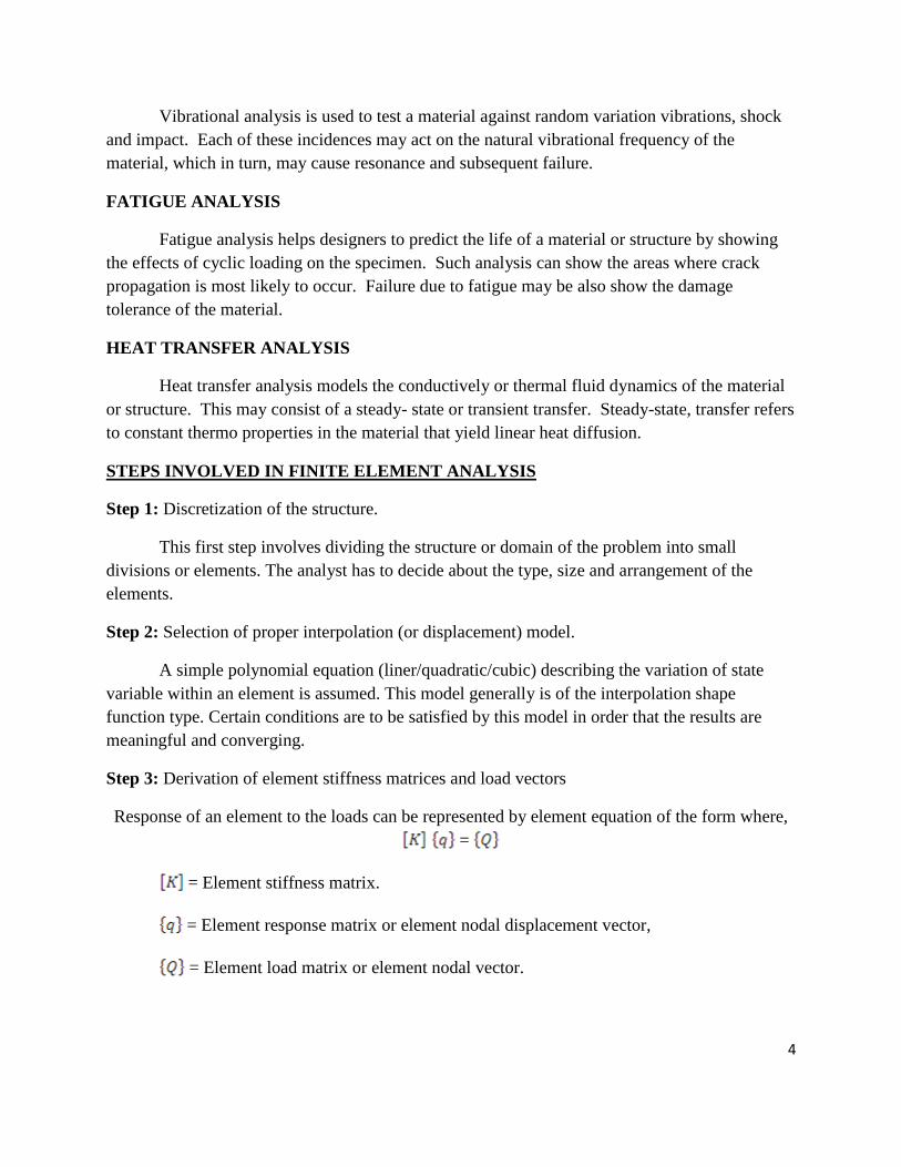
Fig.2.1 PROBLEM DESCRIPTION
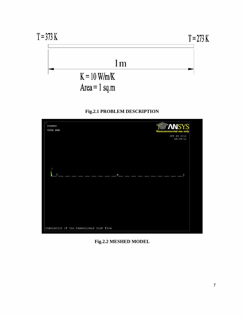
Fig.2.2 MESHED MODEL

8
EX.NO.02: SIMULATION OF ONE DIMENSIONAL HEAT CONDUCTION FLOW
DATE:
AIM:
To perform simulation of one dimensional heat conduction flow of given component
using ANSYS software and plot the results.
PROCEDURE:
Step 1: Set the analysis title
Utility Menu > File > Change the title > simulation of one dimensional heat flow > ok.
Step 2: Define the type of the problem
Main Menu > Preference> Turn on Thermal>ok
Step 3: Define the Type of Elements
Main Menu > Preprocessor > Element Type > Add/Edit/Delete > Add > Link > 3D
conduction 33 > ok>close.
Step 4: Define the Real constant
Main Menu > Preprocessor > Real constant > Add/Edit/Delete > Add > Link > ok >Enter
cross sectional area = 1> ok >close.
Step 5: Define the Material Properties
Main Menu > Preprocessor > Material Props > Material Models > Thermal >
Conductivity > Isotropic > KXX = 10 (Thermal conductivity) > ok >close.
Step 6: Create the Key points
Main Menu > Preprocessor > Modeling > Create > Key points > In Active CS>
Key point
Number
X y Z
1 0 0 0
2 1 0 0
9
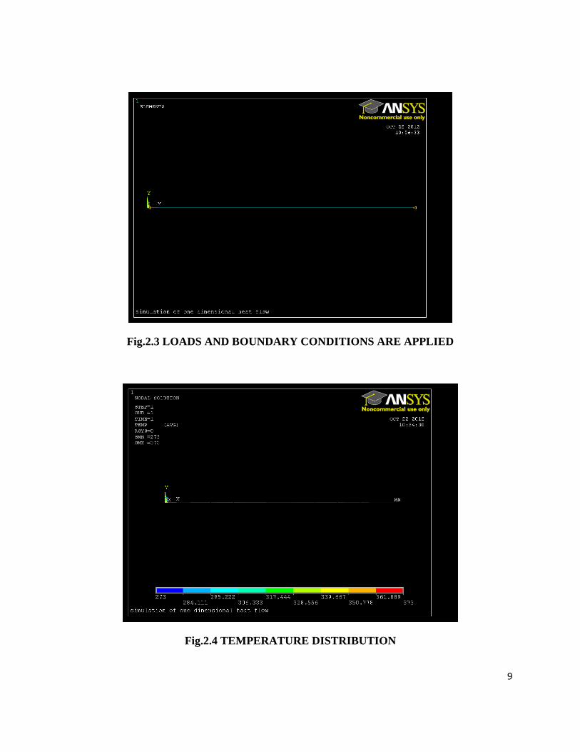
Fig.2.3 LOADS AND BOUNDARY CONDITIONS ARE APPLIED
Fig.2.4 TEMPERATURE DISTRIBUTION

10
Step 7: Create the line
Main Menu > Preprocessor > Modeling > Create > Lines > Lines>Straight Line > pick
the Key Points 1 and 2>ok
Step 8: Mesh Size
Main Menu > Preprocessor > Meshing > Size Cntrls > Manual Size > Lines> All Lines >
Enter Element Edge Length =0.05 > ok.
Step 9: Mesh
Main Menu > Preprocessor > Meshing > Mesh > Lines > Free > Pick All
Step 10: Define Analysis Type
Solution > Analysis Type > New Analysis > Steady-State > ok.
Step 11: Apply the Boundary conditions and loads
Solution > Define Loads > Apply > Thermal > Temperature > On Key points> Select
Key point 1 > ok>select TEMP>Enter Temperature Value = 373.
Solution > Define Loads > Apply > Thermal > Temperature > On Key points> Select
Key point 1 > ok>select TEMP>Enter Temperature Value = 273.
Step 12: Solve the System
Solution > Solve > Current LS > ok >close.
Step 13: Reviewing the Result
Main Menu > General Postproc > Plot Results > Contour Plot > Nodal Solu > DOF
solution > Nodal Temperature >ok
RESULT:
Simulation of one dimensional heat conduction flow of the given component using
ANSYS software are performed and the results are plotted.
11
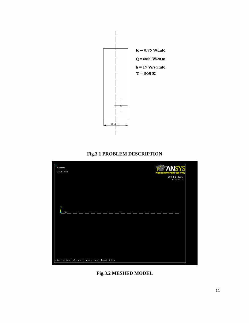
Fig.3.1 PROBLEM DESCRIPTION
Fig.3.2 MESHED MODEL
12
EX.NO.03: SIMULATION OF ONE DIMENSIONAL HEAT FLOW WITH INTERNAL
HEAT GENERATION
DATE:
AIM:
To perform simulation of one dimensional heat flow with internal heat generation of the
given component using ANSYS software and plot the results.
PROCEDURE:
Step 1: Set the analysis title
1. Choose menu path Utility Menu > File > Change Title
2. Type the text thermal analysis of one dimensional heat flow and click on OK.
Step 2: Define the Type of problem
Main Menu > Preferences > select Thermal > ok
Step 3: Define the element types
Main Menu > Preprocessor > Element Type > Add/Edit/Delete > Add > Link > 2D
conduction 32 > ok > Add > Link > 3D conduction 34 > ok > Close.
Step 4: Define the real constants
Main Menu > Preprocessor > Real constants > Add/Edit / Delete > Add > select link 32 >
ok > Enter the Cross-sectional area AREA > Enter 1 > ok > Add > Click on Link 34 > ok > Enter
the Cross-sectional area AREA > Enter 1 > ok
Step 5: Define the material properties
Main Menu>Preprocessor>Material Props> Material Models
Material Model Number 1:
Click Thermal > Conductivity > Isotropic

13
Fig.3.3 LOADS AND BOUNDARY CONDITIONS ARE APPLIED
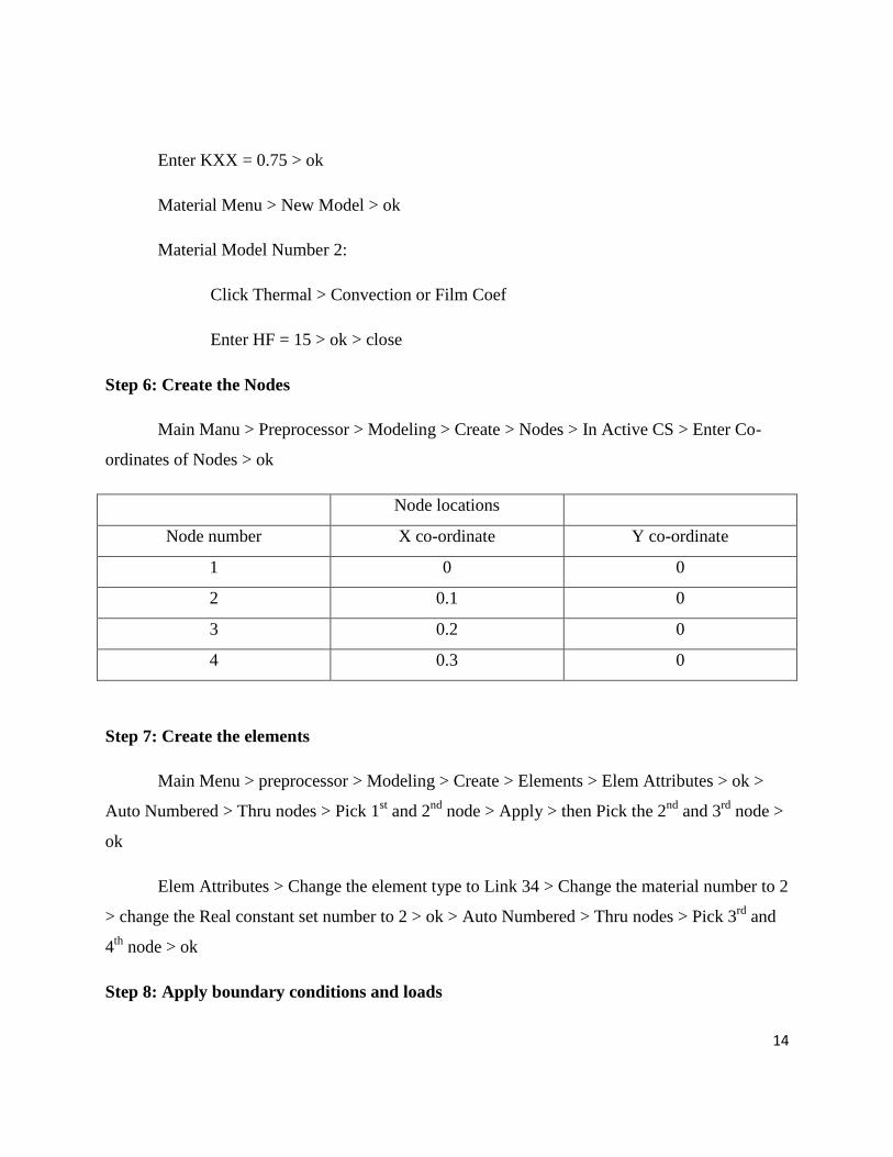
Fig.3.4 TEMPERATURE DISTRIBUTION
14
Enter KXX = 0.75 > ok
Material Menu > New Model > ok
Material Model Number 2:
Click Thermal > Convection or Film Coef
Enter HF = 15 > ok > close
Step 6: Create the Nodes
Main Manu > Preprocessor > Modeling > Create > Nodes > In Active CS > Enter Co-
ordinates of Nodes > ok
Node locations
Node number X co-ordinate Y co-ordinate
1 0 0
2 0.1 0
3 0.2 0
4 0.3 0
Step 7: Create the elements
Main Menu > preprocessor > Modeling > Create > Elements > Elem Attributes > ok >
Auto Numbered > Thru nodes > Pick 1st and 2
nd node > Apply > then Pick the 2
nd and 3
rd node >
ok
Elem Attributes > Change the element type to Link 34 > Change the material number to 2
> change the Real constant set number to 2 > ok > Auto Numbered > Thru nodes > Pick 3rd
and
4th
node > ok
Step 8: Apply boundary conditions and loads
15
Apply Loads
Main Menu > Preprocessor > Loads > Define Loads > Apply > Thermal > Temperature >
On Nodes > Pick the 4th
node > Apply > Click on TEMP and Enter Value = 35 > ok
Apply temperature load
Main Menu > Preprocessor > Loads > Define Loads > Apply > Thermal > Heat Generat
> On Nodes > Pick the 1st, 2
nd and 3
rd nodes > Apply > Enter HGEN Value = 6000 > ok
Step 9: Solve the model
Main Menu > Solution > solve > Current LS > ok > close
Step 10: Review the results
Temperature Distribution
Main Menu > General Postproc > Plot Results > Contour Plot > Nodal Solu > DOF
Solution > Temperature > ok
Main Menu > General Postproc > List Results > Nodal Solu > Select Temperature > ok
RESULT:
Simulation of one dimensional heat flow with internal heat generation of the given
component using ANSYS software are performed and the results are plotted.

16
Fig.4.1 PROBLEM DESCRIPTION
Fig.4.2 MESHED MODEL

17
EX.NO.04: SIMULATION OF TWO DIMENSIONAL STEADY STATE HEAT CONDUCTION FLOW
DATE:
AIM:
To perform simulation of two dimensional steady state heat conduction flow of the
given component using ANSYS software and plot the results.
PROCEDURE:
Step 1: Set the analysis title
Utility Menu > File > Change the title > Conductive Heat Transfer Analysis of a 2D
Component > ok.
Step 2: Define the Type of Elements
Main Menu > Preprocessor > Element Type > Add/Edit/Delete > Add > Solid > Quad
4Node 55 > ok.
Step 3: Define the Material Properties
Main Menu > Preprocessor > Material Props > Material Models > Thermal >
Conductivity > Isotropic > KXX = 10 (Thermal conductivity) > ok >close.
Step 4: Create the Geometry
Main Menu > Preprocessor > Modeling > Create > Areas > Rectangle > By 2 Corners >
X=0, Y=0, Width=1, Height=1 > ok
Step 5: Mesh Size
Main Menu > Preprocessor > Meshing > Size Cntrls > ManualSize > Areas > All Areas >
0.05 > ok.
Step 6: Mesh
Main Menu > Preprocessor > Meshing > Mesh > Areas > Free > Pick All
Step 7: Define Analysis Type
Solution > Analysis Type > New Analysis > Steady-State > ok.
18
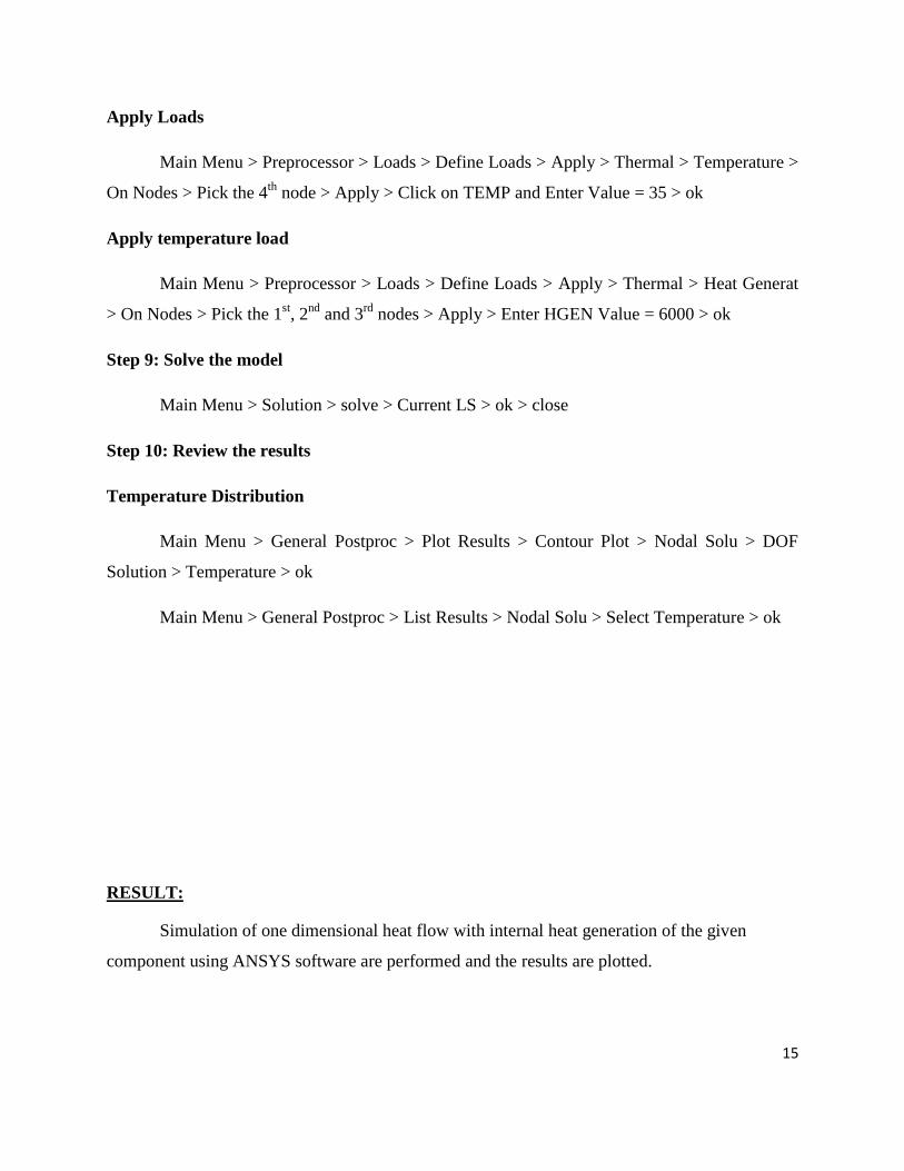
Fig.4.3 LOADS AND BOUNDARY CONDITIONS ARE APPLIED
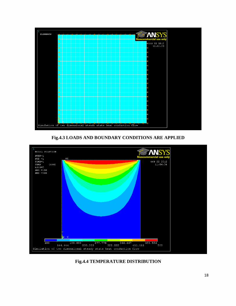
Fig.4.4 TEMPERATURE DISTRIBUTION

19
Step 8: Apply the Boundary conditions and loads
Solution > Define Loads > Apply > Thermal > Temperature > On Nodes > Click the Box
option and draw a box around the nodes on the top line > ok.
Select the Temperature > Enter the constant temperature 500 > ok
Using the same method, constrain the remaining 3 sides to a constant value of 100
Step 9: Solve the System
Solution > Solve > Current LS > ok >close.
Step 10: Reviewing the Result
Main Menu > General Postproc > Plot Results > Contour Plot > Nodal Solu > DOF
solution > Nodal Temperature >ok
RESULT:
Simulation of two dimensional steady state heat conduction flow of the given
component using ANSYS software are performed and the results are plotted.

20
Fig.5.1 PROBLEM DESCRIPTION
Fig.5.2 MESHED MODEL
21
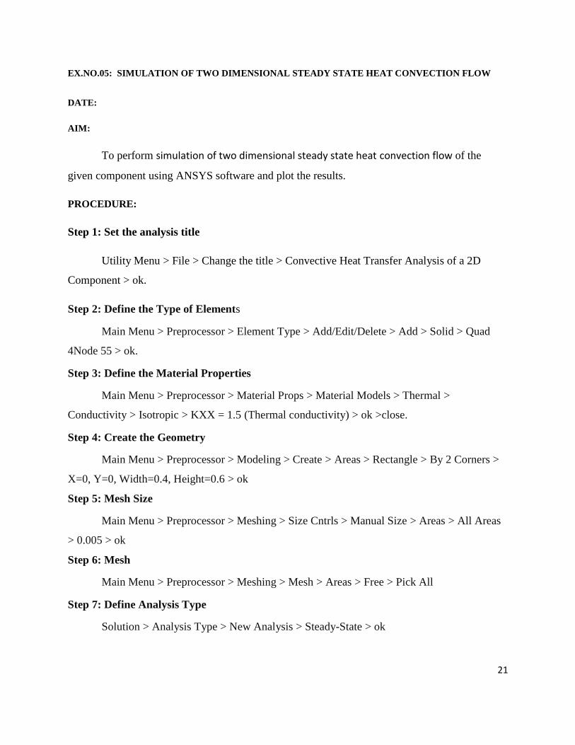
EX.NO.05: SIMULATION OF TWO DIMENSIONAL STEADY STATE HEAT CONVECTION FLOW
DATE:
AIM:
To perform simulation of two dimensional steady state heat convection flow of the
given component using ANSYS software and plot the results.
PROCEDURE:
Step 1: Set the analysis title
Utility Menu > File > Change the title > Convective Heat Transfer Analysis of a 2D
Component > ok.
Step 2: Define the Type of Elements
Main Menu > Preprocessor > Element Type > Add/Edit/Delete > Add > Solid > Quad
4Node 55 > ok.
Step 3: Define the Material Properties
Main Menu > Preprocessor > Material Props > Material Models > Thermal >
Conductivity > Isotropic > KXX = 1.5 (Thermal conductivity) > ok >close.
Step 4: Create the Geometry
Main Menu > Preprocessor > Modeling > Create > Areas > Rectangle > By 2 Corners >
X=0, Y=0, Width=0.4, Height=0.6 > ok
Step 5: Mesh Size
Main Menu > Preprocessor > Meshing > Size Cntrls > Manual Size > Areas > All Areas
> 0.005 > ok
Step 6: Mesh
Main Menu > Preprocessor > Meshing > Mesh > Areas > Free > Pick All
Step 7: Define Analysis Type
Solution > Analysis Type > New Analysis > Steady-State > ok

22
Fig.5.3 LOADS AND BOUNDARY CONDITIONS ARE APPLIED
Fig.5.4 TEMPERATURE DISTRIBUTION
23
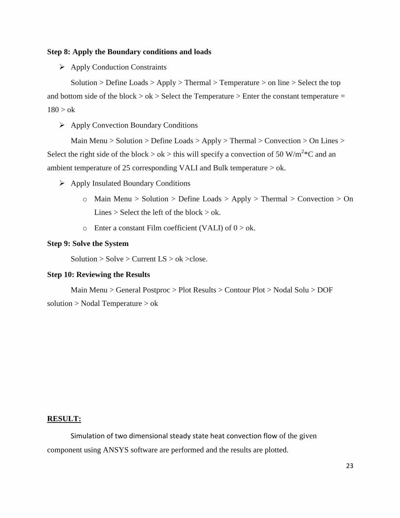
Step 8: Apply the Boundary conditions and loads
Apply Conduction Constraints
Solution > Define Loads > Apply > Thermal > Temperature > on line > Select the top
and bottom side of the block > ok > Select the Temperature > Enter the constant temperature =
180 > ok
Apply Convection Boundary Conditions
Main Menu > Solution > Define Loads > Apply > Thermal > Convection > On Lines >
Select the right side of the block > ok > this will specify a convection of 50 W/m2*C and an
ambient temperature of 25 corresponding VALI and Bulk temperature > ok.
Apply Insulated Boundary Conditions
o Main Menu > Solution > Define Loads > Apply > Thermal > Convection > On
Lines > Select the left of the block > ok.
o Enter a constant Film coefficient (VALI) of 0 > ok.
Step 9: Solve the System
Solution > Solve > Current LS > ok >close.
Step 10: Reviewing the Results
Main Menu > General Postproc > Plot Results > Contour Plot > Nodal Solu > DOF
solution > Nodal Temperature > ok
RESULT:
Simulation of two dimensional steady state heat convection flow of the given
component using ANSYS software are performed and the results are plotted.

24
Fig.6.1 PROBLEM DESCRIPTION
Fig6.2 MESHED MODEL

25
EX.NO.06: SIMULATION OF TWO DIMENSIONAL UNSTEADY STATE (TRANSIENT) HEAT CONDUCTION
FLOW.
DATE:
AIM:
To perform simulation of two dimensional unsteady state heat conduction flow of the
given component using ANSYS software and plot the results.
PROCEDURE:
1. Give example a Title
Utility Menu > File > Change Title>Transient Thermal Conduction
2. Open preprocessor menu
ANSYS Main Menu > Preprocessor
3. Create geometry
Preprocessor > Modeling > Create > Areas > Rectangle > By 2 Corners
X=0, Y=0, Width=1, Height=1
4. Define the Type of Element
Preprocessor > Element Type > Add/Edit/Delete... > click 'Add' > Select Thermal
Mass Solid, Quad 4Node 55
5. Element Material Properties
Preprocessor > Material Props > Material Models > Thermal > Conductivity >
Isotropic > KXX = 5 (Thermal conductivity)
Preprocessor > Material Props > Material Models > Thermal > Specific Heat > C
= 2.04
Preprocessor > Material Props > Material Models > Thermal > Density > DENS =
920
6. Mesh Size Preprocessor > Meshing > Size Cntrls > ManualSize > Areas > All Areas > 0.05
7. Mesh Preprocessor > Meshing > Mesh > Areas > Free > Pick All
Solution Phase: Assigning Loads and Solving
1. Define Analysis Type
Solution > Analysis Type > New Analysis > Transient
2. Set Solution Controls
Solution > Analysis Type > Sol'n Controls
A) Set Time at end of loadstep to 300 and Automatic time stepping to ON.

26
Fig.6.3 LOADS AND BOUNDARY CONDITIONS ARE APPLIED
Fig.6.4 TEMPERATURE DISTRIBUTION
27
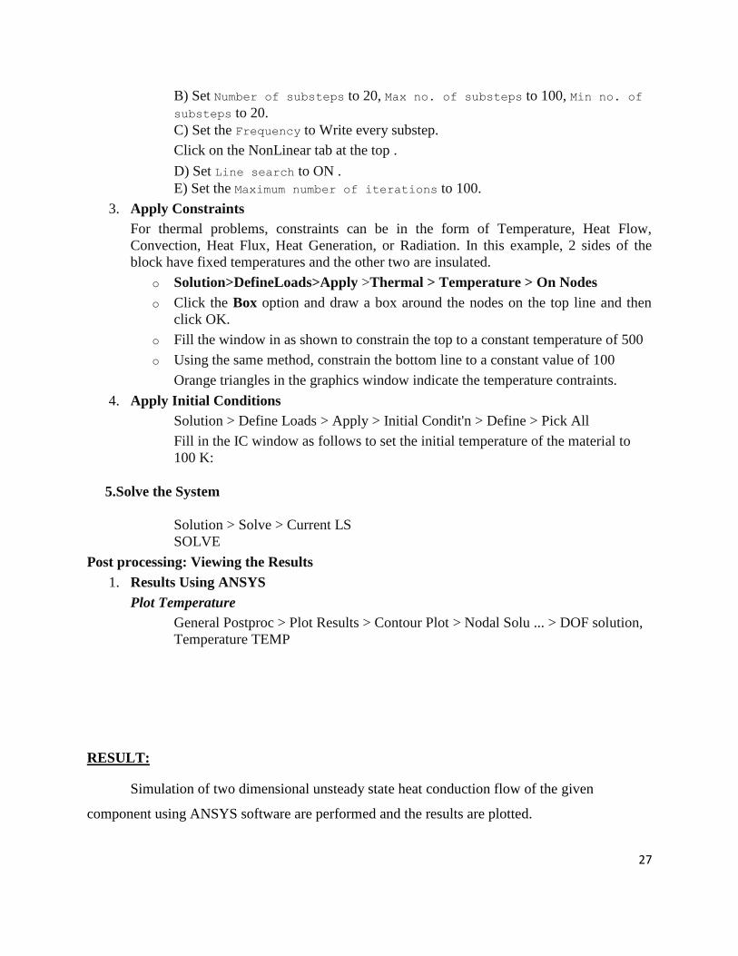
B) Set Number of substeps to 20, Max no. of substeps to 100, Min no. of
substeps to 20.
C) Set the Frequency to Write every substep.
Click on the NonLinear tab at the top .
D) Set Line search to ON .
E) Set the Maximum number of iterations to 100.
3. Apply Constraints
For thermal problems, constraints can be in the form of Temperature, Heat Flow,
Convection, Heat Flux, Heat Generation, or Radiation. In this example, 2 sides of the
block have fixed temperatures and the other two are insulated.
o Solution>DefineLoads>Apply >Thermal > Temperature > On Nodes
o Click the Box option and draw a box around the nodes on the top line and then
click OK.
o Fill the window in as shown to constrain the top to a constant temperature of 500
o Using the same method, constrain the bottom line to a constant value of 100
Orange triangles in the graphics window indicate the temperature contraints.
4. Apply Initial Conditions
Solution > Define Loads > Apply > Initial Condit'n > Define > Pick All
Fill in the IC window as follows to set the initial temperature of the material to
100 K:
5.Solve the System
Solution > Solve > Current LS
SOLVE
Post processing: Viewing the Results
1. Results Using ANSYS
Plot Temperature
General Postproc > Plot Results > Contour Plot > Nodal Solu ... > DOF solution,
Temperature TEMP
RESULT:
Simulation of two dimensional unsteady state heat conduction flow of the given
component using ANSYS software are performed and the results are plotted.

28
Fig.7.1 PROBLEM DESCRIPTION

29
EX.NO.07: SIMULATION OF HEAT FLOW ON TWO DIMENSIONAL AXI-SYMMETRIC PLANE
DATE:
AIM:
To perform simulation of heat flow on two dimensional axi symmetric plane of the given
component using ANSYS software and plot the results.
PROCEDURE:
Step 1: Set the analysis title
1. Choose menu path Utility Menu > File > Change Title
2. Type the text thermal analysis of 2d axi-symmetric component > ok.
Step 2: Define the Type of problem
Main Menu > Preferences > select Thermal > ok
Step 3: Define the element types
Main Menu > Preprocessor > Element Type > Add/Edit/Delete > Add > Solid > Quad 8
node 77 > ok > close.
Step 4: Define the material properties
Main Menu > Preprocessor > Material Props > Material Models > Thermal >
Conductivity > Isotropic
Enter KXX = 0.031 > ok
Step 5: Create the Geometry
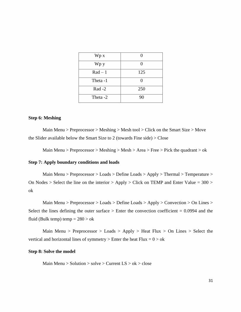
Main Manu > Preprocessor > Modeling > Create > Areas > Circle > Partial Annulus >
Enter the data > ok

30
Fig.7.2 TEMPERATURE DISTRIBUTION
31
Wp x 0
Wp y 0
Rad – 1 125
Theta -1 0
Rad -2 250
Theta -2 90
Step 6: Meshing
Main Menu > Preprocessor > Meshing > Mesh tool > Click on the Smart Size > Move
the Slider available below the Smart Size to 2 (towards Fine side) > Close
Main Menu > Preprocessor > Meshing > Mesh > Area > Free > Pick the quadrant > ok
Step 7: Apply boundary conditions and loads
Main Menu > Preprocessor > Loads > Define Loads > Apply > Thermal > Temperature >
On Nodes > Select the line on the interior > Apply > Click on TEMP and Enter Value = 300 >
ok
Main Menu > Preprocessor > Loads > Define Loads > Apply > Convection > On Lines >
Select the lines defining the outer surface > Enter the convection coefficient = 0.0994 and the
fluid (Bulk temp) temp = 280 > ok
Main Menu > Preprocessor > Loads > Apply > Heat Flux > On Lines > Select the
vertical and horizontal lines of symmetry > Enter the heat Flux = 0 > ok
Step 8: Solve the model
Main Menu > Solution > solve > Current LS > ok > close

32
Step 9: Review the results
Temperature Distribution
Main Menu > General Postproc > Plot Results > Contour Plot > Nodal Solu > DOF
Solution > Temperature > ok
Main Menu > General Postproc > List Results > Nodal Solu > Select Temperature > ok
RESULT:
Simulation of heat flow on two dimensional axi symmetric plane of the given component using
ANSYS software are performed and the results are plotted.
33
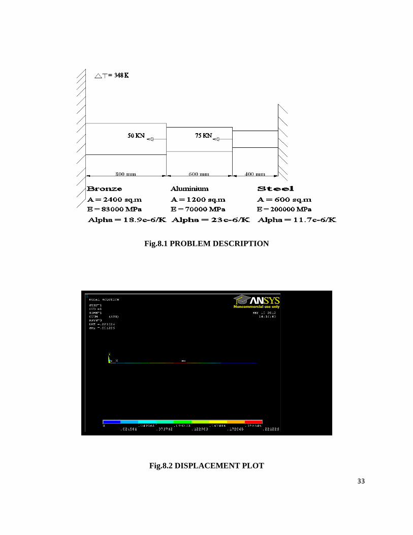
Fig.8.1 PROBLEM DESCRIPTION
Fig.8.2 DISPLACEMENT PLOT

34
EX.NO.08: SIMULATION OF THERMAL STRESS ANALYSIS OF STEPPED SHAFT
DATE:
AIM:
To perform simulation of thermal stress analysis of the given component using ANSYS
software and plot the results.
PROCEDURE:
Step 1: Set the analysis title
1. Choose menu path Utility Menu>File>Change Title
2. Type the text Stepped Bar Analysis > ok.
Step 2: Define the element types
Main Menu>Preprocessor>Element Type>Add/Edit/Delete>Add>Structural>Link>2D
spar>OK>Close.
Step 3: Define the real constants
Main Menu>Preprocessor>Real constants>Add/Edit>Delete>Add>OK
1st element: Cross-sectional area AREA>Enter 2400>OK>Add>OK
2nd
element: Cross-sectional area AREA>Enter 1200>OK>Add>OK
3rd
element: Cross-sectional area AREA>Enter 600>OK>Add>OK>close.
Step 4: Define the material properties
Main Menu>Preprocessor>Material Props> Material Models
Material Model Number 1:
Click Structural > Linear > Elastic > Isotropic
Enter EX = 0.83E5 and PRXY 0.34 > OK
Enter the coefficient of thermal expansion α
Click Structural > Thermal expansion > Secant coefficient > Isotropic
Enter ALPX = 18.9E-6 >OK
Material Menu > New Model > OK

35
Fig.8.3 STRESS PLOT

36
Material Model Number 2:
Click Structural > Linear > Elastic > Isotropic
Enter EX = 0.75E5 and PRXY 0.35 > OK
Enter the coefficient of thermal expansion α
Click Structural > Thermal expansion > Secant coefficient > Isotropic
Enter ALPX = 23E-6 >OK
Material Model Number 3:
Click Structural > Linear > Elastic > Isotropic
Enter EX = 2E5 and PRXY 0.3 > OK
Enter the coefficient of thermal expansion α
Click Structural > Thermal expansion > Secant coefficient > Isotropic
Enter ALPX = 11.7E-6 >OK
Step 5: Create the Nodes
Main Manu > Preprocessor> Modeling > Create > Nodes > In Active CS >Enter Co-
ordinates of Nodes
Node locations
Node number X co-ordinate Y co-ordinate
1 0 0
2 800 0
3 1400 0
4 1800 0
Step 6: Create elements
Main Menu > preprocessor > Modeling > Create > Elements > Elem Attributes > ok >
Auto Numbered > Thru nodes > Pick 1st and 2
nd node > ok
Elem Attributes > Change the material number to 2 > change the Real constant set
number to 2 ok > Auto Numbered > Thru nodes > Pick 2nd
and 3rd
node > ok
Elem Attributes > Change the material number to 3 > change the Real constant set
number to 3 ok > Auto Numbered > Thru nodes > Pick 3rd
and 4th
node > ok

37
Step 7: Apply boundary conditions and loads
Constraint
Main Menu > Preprocessor > Loads > Define Loads > Apply > structural > Displacement
> On Nodes > Pick the 1st node and 4
th node > Apply > All DOF = 0 > ok
Apply Loads
Main Menu > Preprocessor > Loads > Define Loads > Apply > structural >
Force/Moment > On Nodes > Pick the 2nd
node > ok > Force/Moment value = -50e3 in FX
direction > ok > Force/Moment > On Nodes > Pick the 3rd
node > ok > Force/Moment value = -
75e3 in FX direction > ok
Apply temperature load
Main Menu > Preprocessor > Loads > Define Loads > Apply > structural > Temperature
> On Elements > Pick the 1st element, 2
nd element, 3
rd element > ok > Enter Temperature at
location N =75 > ok
Step 8: Solve the model
Main Menu > Solution > solve > Current LS > ok > close
Step 9: Review the results
Displacement
Main Menu > General Postproc > Plot Results > Contour Plot > Nodal Solu > DOF
Solution > Displacement vector sum > ok
Stress
Main Menu > General Postproc > Element Table > Define Table > Add > Select By
sequence num and 1 after LS > ok
Main Menu > General Postproc > Plot Results > Contour Plot > Elem Table > Select LS1
> ok
RESULT:
Simulation of thermal stress analysis of the given component using ANSYS software are
performed and the results are plotted.

38
Fig.9.1 PROBLEM DESCRIPTION
Fig9.2 MESHED MODEL

39
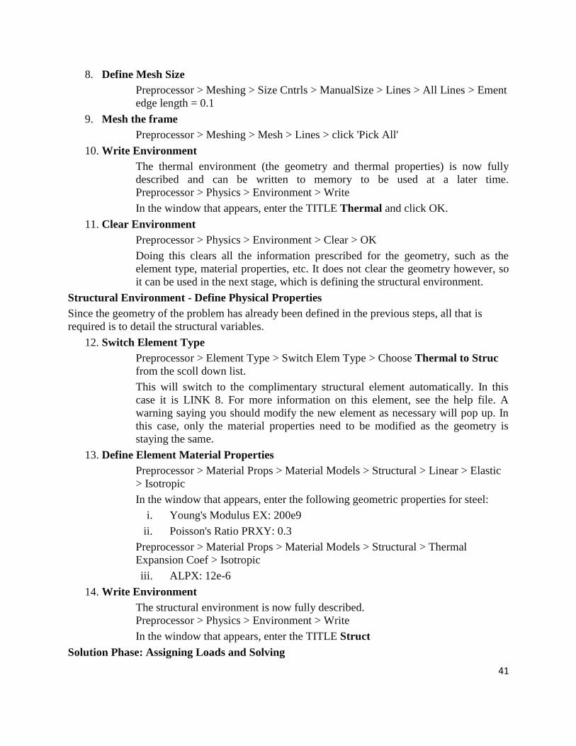
EX.NO.09: SIMULATION OF COUPLED FIELD STRUCTURAL AND THERMAL ANALYSIS
DATE:
AIM:
To perform simulation of coupled field structural and thermal analysis of the given component
using ANSYS software and plot the results.
PROCEDURE:
Thermal Environment - Create Geometry and Define Thermal Properties
1. Give example a Title
Utility Menu > File > Change Title >Enter Coupled Field Thermal Stress
2. Open preprocessor menu
ANSYS Main Menu > Preprocessor
3. Define Keypoints
Preprocessor > Modeling > Create > Keypoints > In Active CS
Keypoint Coordinates (x,y,z)
1 (0,0)
2 (1,0)
4. Create Lines
Preprocessor > Modeling > Create > Lines > Lines > In Active Coord
Create a line joining Key points 1 and 2, representing a link 1 meter long.
5. Define the Type of Element
Preprocessor > Element Type > Add/Edit/Delete
For this problem we will use the LINK33 (Thermal Mass Link 3D conduction)
element.
6. Define Real Constants
Preprocessor > Real Constants... > Add...
In the 'Real Constants for LINK33' window, enter the following geometric
properties:
i. Cross-sectional area AREA: 4e-4
This defines a beam with a cross-sectional area of 2 cm X 2 cm.
7. Define Element Material Properties
Preprocessor > Material Props > Material Models > Thermal > Conductivity >
Isotropic
In the window that appears, enter the following geometric properties for steel:
i. KXX: 60.5

40
Fig.9.3 LOADS AND BOUNDARY CONDITIONS ARE APPLIED
Fig.9.4 TEMPERATURE DISTRIBUTION
41
8. Define Mesh Size
Preprocessor > Meshing > Size Cntrls > ManualSize > Lines > All Lines > Ement
edge length = 0.1
9. Mesh the frame
Preprocessor > Meshing > Mesh > Lines > click 'Pick All'
10. Write Environment
The thermal environment (the geometry and thermal properties) is now fully
described and can be written to memory to be used at a later time.
Preprocessor > Physics > Environment > Write
In the window that appears, enter the TITLE Thermal and click OK.
11. Clear Environment
Preprocessor > Physics > Environment > Clear > OK
Doing this clears all the information prescribed for the geometry, such as the
element type, material properties, etc. It does not clear the geometry however, so
it can be used in the next stage, which is defining the structural environment.
Structural Environment - Define Physical Properties
Since the geometry of the problem has already been defined in the previous steps, all that is
required is to detail the structural variables.
12. Switch Element Type
Preprocessor > Element Type > Switch Elem Type > Choose Thermal to Struc
from the scoll down list.
This will switch to the complimentary structural element automatically. In this
case it is LINK 8. For more information on this element, see the help file. A
warning saying you should modify the new element as necessary will pop up. In
this case, only the material properties need to be modified as the geometry is
staying the same.
13. Define Element Material Properties
Preprocessor > Material Props > Material Models > Structural > Linear > Elastic
> Isotropic
In the window that appears, enter the following geometric properties for steel:
i. Young's Modulus EX: 200e9
ii. Poisson's Ratio PRXY: 0.3
Preprocessor > Material Props > Material Models > Structural > Thermal
Expansion Coef > Isotropic
iii. ALPX: 12e-6
14. Write Environment
The structural environment is now fully described.
Preprocessor > Physics > Environment > Write
In the window that appears, enter the TITLE Struct
Solution Phase: Assigning Loads and Solving
42
15. Define Analysis Type
Solution > Analysis Type > New Analysis > Static
ANTYPE, 0
16. Read in the Thermal Environment
Solution > Physics > Environment > Read
Choose thermal and click OK.
If the Physics option is not available under Solution, click Unabridged Menu at the
bottom of the Solution menu. This should make it visible.
17. Apply Constraints
Solution > Define Loads > Apply > Thermal > Temperature > On Keypoints
Set the temperature of Keypoint 1, the left-most point, to 348 Kelvin.
18. Solve the System
Solution > Solve > Current LS
SOLVE
19. Close the Solution Menu
Main Menu > Finish
It is very important to click Finish as it closes that environment and allows a new
one to be opened without contamination. If this is not done, you will get error
messages.
The thermal solution has now been obtained. If you plot the steady-state temperature on
the link, you will see it is a uniform 348 K, as expected. This information is saved in a
file labelled Jobname.rth, were .rth is the thermal results file. Since the jobname wasn't
changed at the beginning of the analysis, this data can be found as file.rth. We will use
these results in determing the structural effects.
20. Read in the Structural Environment
Solution > Physics > Environment > Read
Choose struct and click OK.
21. Apply Constraints
Solution > Define Loads > Apply > Structural > Displacement > On Keypoints
Fix Keypoint 1 for all DOF's and Keypoint 2 in the UX direction.
22. Include Thermal Effects
Solution > Define Loads > Apply > Structural > Temperature > From Therm
Analy
As shown below, enter the file name file.rth. This couples the results from the
solution of the thermal environment to the information prescribed in the structural
environment and uses it during the analysis.
23. Define Reference Temperature
Preprocessor > Loads > Define Loads > Settings > Reference Temp
For this example set the reference temperature to 273 degrees Kelvin.
43
Fig.9.5 DISPLACEMENT PLOT
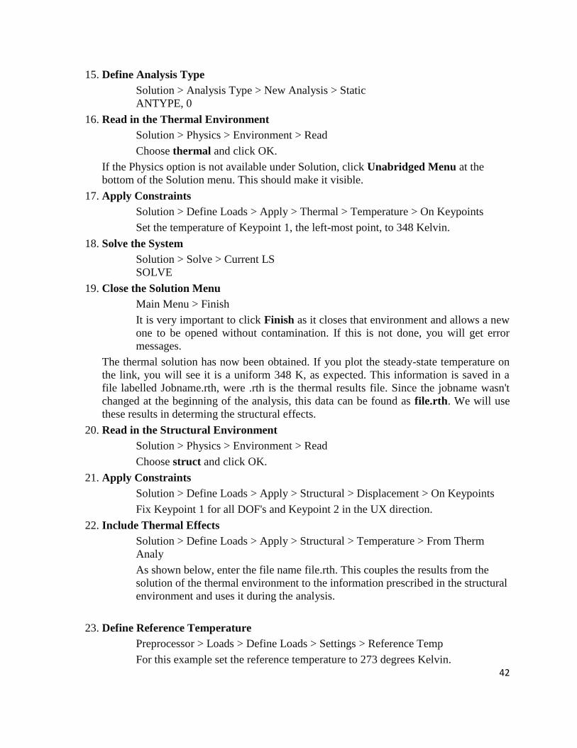
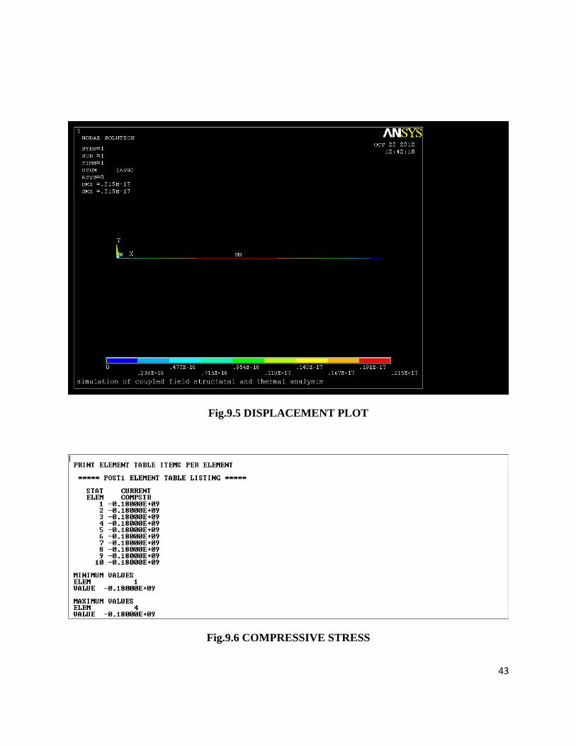
Fig.9.6 COMPRESSIVE STRESS

44
24. Solve the System
Solution > Solve > Current LS
SOLVE
Postprocessing: Viewing the Results
1. Get Stress Data
Since the element is only a line, the stress can't be listed in the normal way.
Instead, an element table must be created first.
General Postproc > Element Table > Define Table > Add
Fill in the window as shown below.
Eff NU for EQV strain = 0
User lable for item = CompStr
Select >By Sequence Num > LS
Enter > LS,1
2. List the Stress Data
General Postproc > Element Table > List Elem Table > COMPSTR > OK
3. Hand Calculations
Hand calculations were performed to verify the solution found using ANSYS:
As shown, the stress in the link should be a uniform 180 MPa in compression.
RESULT:
Simulation of coupled field structural and thermal analysis of the given component using
ANSYS software are performed and the results are plotted.

45
Fig.10.1 PROBLEM DESCRIPTION
Fig.10.2 MESHED MODEL
46
EX.NO.10: SIMULATION OF STEADY STATE FLUID FLOW ANALYSIS
DATE:
AIM:
To perform simulation of steady state fluid flow analysis of the given component using
ANSYS software and plot the results.
PROCEDURE:
Step 1: Set the analysis title
. Utility Menu>File>Change Title>Enter simulation of steady state fluid flow
Step 2: Define type of problem
Main Menu > Preferences, then select FLOTRAN CFD > OK
Step 3: Define the element types
Main Menu > Preprocessor > Element Type > Add/Edit/Delete > Add > FLOTRAN CFD
> 2D FLOTRAN 141 > OK
Step 4: Create Rectangle
Main Menu > Preprocessor > Modeling > Create > Areas > Rectangle > By 2 Corners
Enter (Lower left corner) WP X = 0.0 and Width = 2, Height = 1 > OK
Step 5: Create solid circle
Main Menu > Preprocessor > Modeling > Create > Areas > Circle > Solid Circle. Enter
WP X = 1, WP Y = 0.5 and Radius = 0.2 > OK
Step 6: Subtract Circle from Rectangle
Utility Manu > Plot controls > Numbering > Turn on Areas
Now subtract the circle (Numbered 2) from the rectangle (Numbered 1). (Read the
messages in the window at the bottom of the screen as necessary)
Main Manu > Preprocessor > Modeling > Operate > Booleans > Subtract > Areas > Enter
1>OK>Enter 2 > OK

47
Fig.10.3 LOADS AND BOUNDARY CONDITIONS ARE APPLIED
Fig.10.4 VELOCITY VECTOR PLOT
48
Step7: Meshing
Create a mesh of quadrilateral elements over the area.
Main Manu > Preprocessor > Meshing > Mesh Tool
The Mesh Tool dialog box appears. Close the Mesh Tool box.
Main Menu > Preprocessor > Meshing > Mesh > Areas > Free > Pick the area > OK
Step8: Apply Boundary Conditions and Constraints
Apply the velocity boundary conditions and pressure.
Main Menu > Preprocessor > Loads > Define Loads > Apply > Fluid/CFD > Velocity >
On Lines Pick the left edge of the plate > OK > Enter VX = 1 > OK
Main Menu > Preprocessor > Loads > Define Loads > Apply > Fluid/CFD > Velocity >
On Lines Pick the edges around the cylinder > OK > Enter VX = 0 and VY = 0 > OK
Main Menu > Preprocessor > Loads > Define Loads > Apply > Fluid/CFD > Pressure
DOF > On Lines Pick the top, bottom and right edges of the plate > OK > OK
Step9: Solution.
1. Main Menu > Solution > FLOTRAN Set Up > Fluid Properties > A dialog box appears in
that select against density as liquid and against viscosity as liquid. > OK
Then another dialog box appears in that enter the value of density = 1000 and viscosity
value = 0.001 > OK
2. Main Menu > Solution > FLOTRAN Set Up > Execution Ctrl > a dialog box appears in
that Enter in the first row “Global iterations EXEC” = 200
3. Main Menu > Solution > Run FLOATRAN
When the solution is complete, close the „Solution is Done!‟ window.
Step10: Post processing
We can now plot the results of this analysis and also list the computed values.
Main Menu > General Postproc > Read Results > List Set
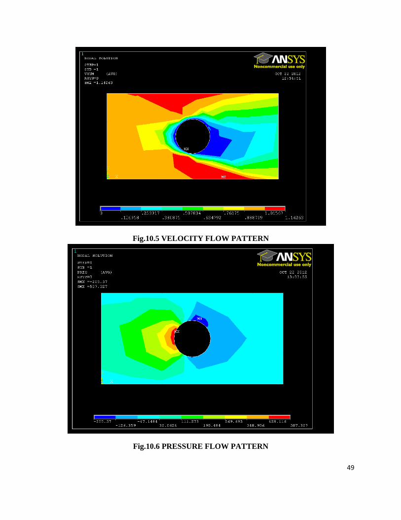
General Postproc > Plot Results > Contour Plot > Nodal Solu
Select DOF Solution and Fluid Velocity and click OK
49
Fig.10.5 VELOCITY FLOW PATTERN
Fig.10.6 PRESSURE FLOW PATTERN
50
Next, go to Main Menu > General Postproc > Plot Results > Vector Plot > Predefined.
General Postproc > Plot resulst > Contour Plot > Nodel Sol
Select DOF Solution and Pressure and Click OK.
RESULT:
Simulation of steady state fluid flow analysis of the given component using ANSYS
software are performed and the results are plotted.
51
EX.NO.11: STUDY OF BASICS OF MATLAB
DATE:
AIM:
To study the basic operations, commands and codes of MATLAB.
INTRODUCTION
This chapter is a brief introduction to MATLAB ( an abbreviation of MATrix LABoratory)
basics, registered trademark of computer software, version 4.0 or later developed by the Math
Works Inc. The software is widely used in many of science and engineering fields, MATLAB is
an interactive program for numerical computation and data visualization. MATLAB is supported
on unix, macintosh, and windows environments. for more information on MATLAB, contact the
Math Work.com. a windows version of MATLAB is assumed here. The syntax is very similar
for the dos version.
MATLAB integrates mathematical computing, visualization, and a powerful language to provide
a flexible environment for technical computing. The open architecture makes it easy to use
MATLAB and its companion products to explore data, create algorithms, and create custom
tools that provides early insights and competitive advantages.
Known for its highly optimized matrix and vector calculations, MATLAB offers on intuitive
languages for expressing problems and their solutions both mathematically and visually.
Typically uses include:
o Numeric computation and algorithm development
o Symbolic computation (with the built-in symbolic math function)
o Modeling, simulation, and prototyping
o Data analysis and signal processing
o Engineering graphics and scientific visualization
In this chapter, We will introduce the MATLAB environment, We will learn how to create , edit,
save, run, and debug m-files (ASCII files with series of MATLAB statements). We will see how
to create arrays (matrices and vectors), and explore the built-in MATLAB linear algebra
functions for matrix and vector multiplication, do not cross products, transpose, determinates,
and inverses and for the solution linear equations. MATLAB is based on the language c, but is
generally much easier to use. We will also see how to program logic constructs and oops in
MATLAB, how to use subprograms and functions, and how to use comments (%) for explaining
the programs and tabs for easy readability, and how to print and plot graphics both two and three
dimensional MATLAB's functions for symbolic mathematics are presented. use of these
functions to perform symbolic operations, to develop closed from expression for solution to
52
algebraic equations, ordinary differential equations , and system equation for presented .
Symbolic mathematics can be used to determine analytical expression for the derivative and
integral of an expressions.
Starting and Quitting MATLAB
To start MATLAB click on the MATLAB icon or type in MATLAB , followed by pressing the
enter or return key at the system prompt. the screen will produce the MATLAB prompt >>(or
EDU>>), which indicates that MATLAB is waiting for a command to be entered.
in order to quit MATLAB, type quit or exit after prompt , followed by pressing the enter or
return key.
Display Windows
MATLAB has three display windows. They are
1. A command Windows which is used to enter commands and data to display plots and graphs.
2.A Graphic Windows which is used to display plots and graphs
3. A Edit window which used to crate and modify m-files. m-flies are the files that contain a
program are script of MATLAB commands.
Entering Commands
Every command has to be followed by a carrier return <cr> (enter key) in order that the
command can be executed. MATLAB command are case sensitive and lower case letters are
used throughout.
To execute an M-files (such as Project_1.m ). simply enter the name of the file without its
extension (as in project_1).
MATLAB expo
In order to see some of the, MATLAB capabilities , enter the demo command this will initiate
the MATLAB expo , MATLAB Expo is a graphical demonstration environment that shows the
some of the different type of operations which can be conducted with MATLAB.
Abort
In order to abort a command in MATLAB , hold down the control key and press c to generate a
local abort with MATLAB.
The Semicolon (;)

53
If a semicolon (;) is typed at the end of the command , the output of the command is not
displayed.
Typing %
When percent symbol (%) is typed in the beginning of a line, the line is designated as a
command . W.....hen the enter key is pressed , the line is not executed.
The clc Command
The typing clc command and pressing enter cleans the command windows. once the clc
command is executed a clear windows is displayed.
Help
The MATLAB has a host of bulit in fuctions. For complete list , refer to MATLAB user's guide
or refer to online Help . To obtain the help on the particular topic in the list, eg. inverse , type
help inv.
Statements and Variables
Statements have the form
>> variable = expression
the equal sign implies the asssign ment of the expression to the variable. for instance to enter a
2x2
matrix with a variable name A, we write
>> A= ={1 2 ; 3 4 } <ret>
the statement is executed after the carriage return (or enter ) key is pressed to display
A=
1 2
3 4
ARITHMATIC OPERATION
The symbols for arithmetic operations with scalars are summarized below in tables 2.1
Table

54
Arithmatic operation Symbol Example
Addition + 6+3=9
Subtraction - 6-3=3
Multiplication x 6*3=18
Right division / 6/3=2
Left division \ 6\3=3/6=1/2
Exponentiation ^ 6^3(63=261)
Table Common Math Functions
Function Description
abs(x) Computes the absolute value of x
sqrt(x) Computes the square root of x
round(x) Rounds x to nearest integer
fix(x) Rounds (or truncates ) x to the nearest integer
floor(x) Rounds x to the earest integer toward -∞
ceil(x) Rounds x to the earest integer toward ∞
sign(x) Returns a value of -1 if x is less than 0, a value
of 0 if equals 0, and a value of 1 otherwise
rem(x,y) Returns the remainder of x/y. for example,
rem(25,4) is 1, and rem (100,21) is 16. This
function is also called a modulus function
exp(x) Computes ex, where e is the base for natural
logarithms , or approximately 2.718282
log(x) Computes ln x, the atural logarithm of x to the
base e.
log10(x) Computes log10 x, the common logarithm of x
to the base 10

55
Table Exponential Functions
Function Description
exp(x) Exponential (ex)
log(x) Natural logarithm
log10(x) Base 10 logarithm
sqrt(x) Square root
Table trigonometric and hyperbolic functions
Function Description
sin(x) Computes the sine of x, where x is in radians
cos (x) Computes the cosine of x, where x is in
radians
tan(x) Computes the tangent of x, where x is in
radians
asin(x) Computes the arcsine or inverse sine of x,
where x is must be between -1 and 1. the
function returns an angle oin radians between
- and
acos(x) Computes the arccosine or inverse cosine of
x, where x is must be between -1 and 1. the
function returns an angle oin radians between
0 and π
atan(x) Computes the arctangent or inverse tangent
of x. the function returns an angle oin radians
between - and

56
atan2(y,x) Computes the arctangent or inverse tangent
of y/x. the function returns an angle oin
radians between x and y
sinh(x) computes the hyperbolic sine of x,which is
equal to ex-e
-x/2
cosh(x) computes the hyperbolic cosine of x,which is
equal to ex+e
-x/2
tanh(x) compute the hyperbolic tangent of x, which is
equal to sinhx/coshx
asinh(x) compute the hyperbolic sine of x, which is
equal to x+
acosh(x) compute the hyperbolic cosine of x, which is
equal to x+
atanh(x) compute the inverse hyperbolic tangent of x,
which is equal to
Table on- line help
function description
help lists topics on which help is available
helpwin opens the interactive help window
helpdesk opens the web browser based help facility
helptopic provides help on topic
lookfor string lists help topics containing string
demo runs the demo program
Workplace information
function description

57
who lists variables currently in the workplace
whos lists variables currently in the workplace with
their size
what lists m, mat, and mex- files on the disk
clear clears the workplace, all variables are
removed
clear x y z clears only variables x, y, and z.
clear all clears all variables and functions from
workplace
mlock fun looks fun so that clear cannot remove it
munlock fun unlocks function fun so that clear can remove
it
clc clear command window, command histo0ry
is lost
home same as clc
clf clears figure window
ARRAYS
An array ia a list of numbers arranged in rows and or columns. a one dimensional arrray is a row
or a column of numbers and a two dimensional array has a set of numbers arranged in rows and
columns. an array operation is performed element by element.
ROW VECTOR
A vector is a row or column of elements.
In a row vector the elements are entered with a space or a comma between the elements inside
the square brackets. for example,
x=[7 -1 2 -5 8]
COLUMN VECTOR

58
In a column vector the elements or enterd with asemicolun between the elements inside the
square brackets. for example,
x= [7; -1; 2; -5; 8;]
MATRIX
A matrix is a two dimensional array which has numbers in rows and columns. A matrix is a
enterd a row wise with consecutive elements of a rows sepearted by a space or a comma, and the
rows seperated by a semi colon or carriage returns, the entire matrix is enclosed with in square
brackets, in the elements of matrix may be real numbers or comples numbers. for example to
enter the matrix
A=
The mat lab input command is
A=[1 3 -4; 0 -2 8]
similarly for complex number elements of a matrix B
B=
The matlab input command is
B=[-5*x log(2*x)+7*sin(3*y); 3i 5-13i ]
ADDRESING ARRAYS
A colon can be used in mat lab to addres a range of elements in a vector or a matrix
COLON FOR A VECTOR
Va(:) - refers to all the elements of the vector Va (either a row or a column vector)
Va(m:n) - refers to a elements m through n of the vector Va
For instance
>> V =[2 5 -1 11 8 4 7 -3 11]
>> U= V(2:8)

59
U= 5 -1 11 8 4 7 -3 11
COLUMN FOR A MATRIX
Table gives the use of colon in addresing arrays in a matrix\
colon use for a matrix
Command Description
A(:,n)
A(n,:)
A(:,m:n)
A(m:n, :)
A(m:n, p:q)
refers to the elements in alll the rows of a coloumn n of the matrix A
Refers to the elements in all the columns of row n of the matrix A
Refers to the elements in all the rows between coloumns m and n of the
matrix A
Refers to the elements in all the coloumns between rows m and n of the
matrix A
Refers to the elements in all the rows m through n and coloumns p through
q of the matrix A
Adding elements to a vector or a matrix
A variable that exists as a vector, or a matrix, can be changed by adding elements to it. Addition
of elements is done by assigining values of the additional elements, or by appending existing
varibales . rows and or coloumns can be added to an existing matrix by assigning values to the
new rows or columns.
DELETING ELEMENTS
An element, or a range of elements. of an existing variable can be deleted by reassigning blanks
to these elements. this is done simply by the use of square brackets with nothing typed in
between them.
BUILT-IN FUNCTIONS
Some of the built-in functions available in MATLAB for managing and handling arrays as listed
Built-in functions for handling arrays
Function Description

60
Length(A) Returns the number of elements in the vector A.
Size(A) Returns a row vector [m,n], Where m and n are the size mxn of the array A.
Reshape(A,m,n) Rearrange a matrix A that has r rows and a coloumns to have m rows and n
columns r times s must be equal to m times n.
Diag(v) When v is a vector, create a square matrix with the elements of v in the
diagonal
Ia (A0 When A is a matrix, creates a vector from the diagonal of A.
2.10 OPERATIONS WITH ARRAYS
We consider here matrices that have than one row and more than one column
ADDITION AND SUBTRACTION OF MATRICES
The addition ( the sum) or the subtraction (the difference) of the two arrays is obtained by adding
or subtracting their corresponding elements. These operations are performed with arrays of
identiacal size (same number of rows and columns.)
for example if A and B are two arrays (2x3 matrices)
A = and B=
then, the matrix addition (A+B) is obtained by adding A and B is
DOT PRODUCT
The product is a scalar computed from two vectors of the same size. the scalar is the sum of the
products of the values in corresponding positions in the vectors.
for n elements in the vectors A and B
dot product = A.B =
61
dot (A,B) computes the dot product of A and B. if A and B are matrices , the dot product is a
vector containing the dot products for the corresponding columns of A and B
ARRAY MULTIPLICATION
The value in positon ci,j of the product C of two matrices , A and B, is the dot product of row I of
the first matrix and column j of the second matrix:
Ci,j =
Array division
The division operation can be explained by means of the identity matrix and the inverse matrix
operation .
Identity matrix
An identity matrix is a square matrix in which all the diagonal elements are 1‟ds, and the
remaining elements are 0‟s. if a matrix A is square, then it can be multiplied by the identity
matrix, I, from the left or from the right
AI=IA=A
Inverse of a matrix
The matrix B is the inverse of the matrix A if when the two matrices are multiplied the product is
the identity matrix. Both matrices A and B must be square and the order of the multiplication can
be AB or BA
AB=BA=I
Transpose
The transpose of a matrix is a new matrix in which the rows of the orginal matrix are the
columns of the new matrix. The transopse of a given matrix A is denoted by AT. in MATLAB,
the transpose of the matrix A is denoted by A‟
Determinant
A determinant is a scalar computed from the entries in a square matrix. For a 2x2 matrix A, the
determinant is
|A| = a11a22-a21a12

62
MATLAB will compute determinant of a matrix using the det function:
Det (A) computes the determinant of a suare matrix A .
Array Division
MATLAB has two types of array divisions, which are the left division and the right
division.
Left division
The left division is used to solve the matrix equation Ax=B where x and B are column
vectors.
Multiplying both sides of this equation by inverse of A, A-1
, we have
A-1
Ax=A
-1 B
or Ix = ᵪ = A-1
B
In MATLAB, the above equation is written by using the left division character:
ᵪ = A\B
Right Division
The Right division is used to solve the matrix equation xA = B where x and B are row
vectors.
Multiplying both sides of this equation by the inverse of A, A-1
, we have
ᵪ.A A-1
= B.A-1
ᵪ = B . A-1
or
In MATLAB, this equation is written by using the right division character:
ᵪ = A / B
Eigenvalues and Eigenvectors
Consider the following equation,

63
AX = λX
Where A is an n X n square matrix, X is a column vector with n rows and λ is a scalar.
The values of λ for which X are nonzero are called the eigenvalues of the matrix A, and
The corresponding values of X are called the eigenvalues of the matrix A .
Equation (2.1) can also be used to find the following equation
(A – λI) X = 0
Where IIs an n x n identity matrix. Equation (2.2) corresponding to a set of homogeneous
Equation and has nontrivial solutions only if the determinant is equal to zero, or
│A – λI│ = 0
Equation (2.3) is known as the characteristic equation of the matrix A. The solution to
Eq. (2.3) gives eigenvalues of the matrix A.
MATLAB determines both the eigenvalues and ei8genvectors for a matrix A.
eig (A) Computes a column vector containing the eigenvalues of A.
[Q,d] = eig(A)Computes a square matrix Q containing the eigenvectors of A as columns
And a square matrix d containing the eigenvalues (λ) of A on the diagonal.
The values of Qand d are such thatQ*Qis the identity matrix and A*X
Equals (λ) times X.
Element – by element operations
Arithmetic operations
Matrix operators
Array operators
+ Addition
+ Addition

64
- Subtraction
* Multiplication
^ Exponentiation
/ Left division
\ Right division
- Subtraction
.* Array Multiplication
.^ Array Exponentiation
./ Array Left division
.\ Array Right division
Matrix Division
The solution to the matrix equation AX = B is obtained using matrix division , or X =
A/B. The vector X then contains the values of x
Matrix Inverse
For the solution of the matrix equation AX = B , we premultiply both sides of the
equation by A-1
A-1
AX = A-1
B
Or IX = A-1
B
Where I is the identity matrix
Hence X = A-1
B
In MATLAB , we use the command x = inv (A)*B. Similarly , for XA = B, we use the
command x = B*inv (A)

65
The basic computional unit in MATLAB is the matrix . A matrix expression is enclosed
in square brackets , [ ].Blanks or commas seprate the column elements , and semisolons or
carriage return separate the rows.
Matrix operations require that the matrix dimensions be compatible . If A is an n * m and
B is a p * r then A ± B is allowed only if n = p and m = r . similarly , matrix product A*B is
allowed only if m = p.
SCRIPT FILES
A script is a sequence of ordinary statement and functions used at the command prompt
level. A Script is invoked at the command prompt level by typing the file-name or by using the
pull down menu. Script can also invoke other scripts.
The commands in the command window cannot be saved and executed again. Also, the
command window is not interactive. To overcome these difficulties, the procedure is first to
create a file with a list of command, save it, and then run the file. In this way the commands
contained are executed in the order they are listed when the file is run. In addition, as the need
arises, one can change or modify the commands in the file, the file can be saved and run again
the file that are used in this fashion are known as script file. Thus, a script file is a text file that
contains a sequence of MATLAB commands. Script file can be edited (corrected and/or
changed)and executed many times.
Creating and Saving a script File
Any text editor can be used to create script files. In MATLAB script file are created and edited in
the Editor/Debugger window .this window can be opened from the command window, select file,
New, and then M-file. Once the window is open, the commands of the script file are typed line.
The commands can also be typed in any text editor or word processor program and then copied
and pasted in the edit/debugger window. The second type of M-File is the function file. Function
file enables the user to extend the basic library function by adding one‟s own computational
procedures. Function M-files are expected to return one or more results. Script files and function
files may include reference to other MATLAB toolbox routines.
MATLAB function file begins with a header statement of the form:
Function (name of result or results)=name (argument list)
Before a script file can be executed it must be saved. All script files must be saved with the
extension “.m”. MATLAB refers to them as m-files. When using MATLAB M-files editor, the
files will automatically be saved with the “.m” extension. If any other text editor is used, the file
must be saved with the “.m” extension, or MATLAB will not be able to find and run the script
file. This is done by choosing save As… from the file menu, selecting a location, and entering a
66
name for the file. The names of user defined variables, predefined variables, MATLAB
commands or functions should not be used to name script files.
Running a script file
A script file can be executed either by typing its name in the command window and then
pressing the enter key, directly from the Editor Window by clicking on the Run icon. File The is
assumed to be in the current directly, or in the search path.
Input to a script file
There are three ways of assigning a value to variable in a script file.
1. The variable is defined and assigned value in the script file
2. The variable is defined and assigned value in the command windows
3. The variable is defined in the script file, but a specified value
Output commands
There are two commands that are commonly used to generate output. They are the disp
and fprintf commands.
1. The disp command
The disp command displays the elements of a variable without displaying the name of the
variable, and displays text
2. The fprintf command
The fprint command displays output (text and data) on the screen or saves it to a file.
The output can be formatted using this command
PROGRAMMING IN MATLAB
One most significant of MATLAB is its extendibility through user-written programs such as the
M-files. M-files are ordinary ASCII text files written in MATLAB language. A function file is a
subprogr
Relational and logical operators
A relational operator compares two numbers by finding whether a comparison statement is true
or false. A logical operator examines true/false statements and produces a result which is true or
false according to the specific operator. Relational and logical operators are used in mathematical
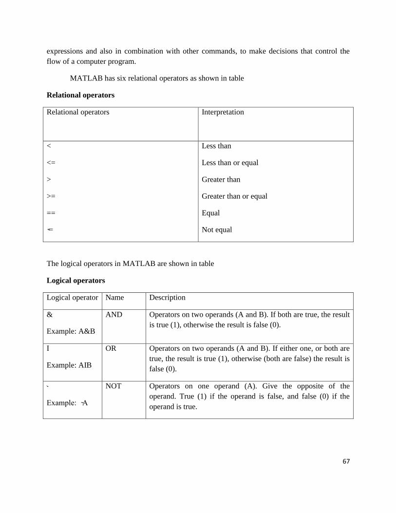
67
expressions and also in combination with other commands, to make decisions that control the
flow of a computer program.
MATLAB has six relational operators as shown in table
Relational operators
Relational operators
Interpretation
<
<=
>
>=
==
=
Less than
Less than or equal
Greater than
Greater than or equal
Equal
Not equal
The logical operators in MATLAB are shown in table
Logical operators
Logical operator Name Description
&
Example: A&B
AND Operators on two operands (A and B). If both are true, the result
is true (1), otherwise the result is false (0).
I
Example: AIB
OR Operators on two operands (A and B). If either one, or both are
true, the result is true (1), otherwise (both are false) the result is
false (0).
˞
Example A
NOT Operators on one operand (A). Give the opposite of the
operand. True (1) if the operand is false, and false (0) if the
operand is true.

68
Order of precedence
The following table shows the order of precedence used by MATLAB.
Precedence Operation
1 (highest)
2
3
4
5
6
7
8 (lowest)
Parentheses (If nested parentheses exist, inner have precedence).
Exponentiation
Logical NOT ( )
Multiplication, Division.
Addition, Subtraction.
Relational operators ( , , =, =,==, =)
Logical AND (&).
Logical OR (I)
2.16.3 Built-in logical Functions
The MATLAB built-in functions which are equivalent to the logical operators are:
And (A, B) Equivalent to A & B
Or (A, B) Equivalent to A I B
Not (A) Equivalent to A
List of the MATLAB logical built-in functions are described in table
GRAPHICS
MATLAB has many commands that can be used to create basic 2-D plots, overlay plots,
specialized 2-D plots, 3-D plots, mesh, and surface plots.
Basic 2-D plots
The basic command for producing a simple 2-D plots is
69
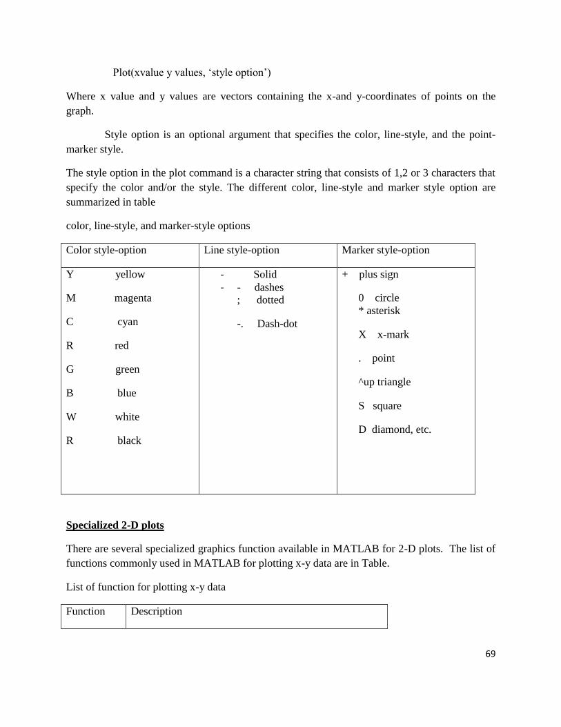
Plot(xvalue y values, „style option‟)
Where x value and y values are vectors containing the x-and y-coordinates of points on the
graph.
Style option is an optional argument that specifies the color, line-style, and the point-
marker style.
The style option in the plot command is a character string that consists of 1,2 or 3 characters that
specify the color and/or the style. The different color, line-style and marker style option are
summarized in table
color, line-style, and marker-style options
Color style-option Line style-option Marker style-option
Y yellow
M magenta
C cyan
R red
G green
B blue
W white
R black
- Solid
- - dashes
; dotted
-. Dash-dot
+ plus sign
0 circle
* asterisk
X x-mark
. point
^up triangle
S square
D diamond, etc.
Specialized 2-D plots
There are several specialized graphics function available in MATLAB for 2-D plots. The list of
functions commonly used in MATLAB for plotting x-y data are in Table.
List of function for plotting x-y data
Function Description

70
Area
Bar
Barh
Comet
Compass
Contour
Contourf
Errobar
Feather
Fill
Fplot
Hist
Loglog
Pareto
pcolor
Creates a filled area plot.
Creates a bar graph.
Creates a horizontal bar graph.
Makes an animated 2-D plots.
Creates arrow graph for complex number.
Makes contour plots
Makes filled contour plots.
Plots a graph and puts error bars.
Makes a feather plot.
Draws filled polygons of specified color.
Plots a function of a single variable.
Makes histograms.
Creates plots with log scale on both x and y axes.
Makes pareto plots.
Makes pseudo color plot matrix
command Description
Pie
Plotyy
Plotmatrix
Polar
Quiver
Rose
Scatter
Creates a pie chart.
Makes a double y-axis plot.
Makes a scatter plot of a matrix.
Plots curves in polar coordinates.
Plots vector fields.
Makes angled histograms.
Creates a scatter plot.

71
Semilogx
Semilogy
Stairs
stem
Makes semilog plot with log scale on the x-axis.
Makes semilog plot with log scale on the y-axis.
Plots a stair graph.
Plots a stem graph.
Overlay plots
There are three ways of generating overlay plots in MATLAB, they are
(a)Plot command
(b)Hold command
(c)Line command
(a)Plot command. Example E2.7(a) shows the use of plot command used with matrix
argument, each column of the second argument matrix plotted against the corresponding column
of the first argument matrix.
(b)Hold command . invoking hold on at any point during a session freezes the current plot in
the graphics window. All the next plots generated by the plot command are added to the exiting
plot. See Example E2.7(a).
(c)Line command. The line command takes a pair of vectors (or a triplet in 3-D) followed by
a parameter name/parameter value pairs as argument. For instance, the command: line (x data, y
data, parameter name, parameter value) adds lines to the existing axes. See Example E2.7(a).
3-D plots
MATLAB provides various options for displaying three-dimensional data. They include line and
wire, surface, mesh plots, among many others. More information can be found in the Help
window under plotting and Data visualization. Table lists commonly used function.
Functions used for 3-D graphics
command Description
Plot3
Plots three-dimensional graph of the trajectory of a set of thee
parametric equations x(t), y(t), and z(t) can be obtained using
plot3(x,y,z).

72
Meshgrid
Mesh(X,Y,z)
If x and y are two vectors containing a range of points for the evaluation
of a function, [X,Y]=meshgrid(x,y) returns two rectangular matrices
containing the x and y values at each point of a two-dimensional grid.
If X and Y are rectangular arrays containing the values of the x and y
coordinates at each point of a rectangular grid, and if z is the value of a
function evaluated at each of these points, mesh(X,Y,z) will produce a
three-dimensional perspective graph of the points. The same results can
be obtained with mesh(x,y,z) which can also b used.
command Description
Mesch,meshz
Surf
Surfc
Colormap
If the xy grid is rectangular, these two function are merely variations of
the basic plotting program mesh, and they operate in an identical
fashion. Meshc will produce a corresponding contour plot drawn on the
xy plane below the three dimensional figure, and meshz will add a
vertical wall to the outside features of the figures drawn by mesh.
Produces a three-dimensional perspective drawing. Its use is usually to
draw surfaces, as opposed to plotting functions, although the actual
tasks are quite similar. The output of surf will be a shaded figure. If
row vectors of length n are defined by x=y cos and y=r sin , with 0_<
2they correspond to a circle of radius r. if r is column vector equal to
r=[0 1 2]‟;then z=r*ones(size(x)) will be a rectangular, 3 x n,arrays of
0‟s and 2‟s, and surf(x,y,z) will produce a shaded surface bounded by
three circles; i.e., a cone.
This function is related to surf in the same way that meshc is related to
mesh.
Used to change the default coloring of a figure. See the MATLAB
reference manual or the help file.
Controls the type of color shading used in drawing figures. See the
MATLAB reference manual or the help file.
View(az,el) controls the perspective view of a three-dimensional plot.
The view of the figure is from angle ”el” above the xy plane with the
coordinate axes (and the figure) rotated by an angle “az” in a clockwise
direction about the z axis. Both angles are in degrees. The default

73
View
Axis
Contour
Plot3
values are az=371/2 and el=30
Determines or changes the scaling of p plot. If the coordinate axis
limits of a two dimensional of three-dimensional graph are contained in
the row vector r=[] axis will return the values in this vector, and axis(r)
can b used to alter them. The coordinate axes can be turned on and off
with axis(„on‟) and axis(„off‟). A few other string constant inputs to
axis and their effects are given below:
Axis(„equal‟) x and y scaling are forced to be the same.
Axis(„square‟) The box formed by the axes is square.
Axis(„auto‟) Restores the scaling to default settings.
Axis(„normal‟) Restoring the scaling to full size, removing any effects
of
square or equal settings.
Axis(„image‟) Alters the aspect ratio and the scaling so the screen
pixels are
square shaped rather than rectangular.
The use is contour(x,y,z). A default value of N=10 contour lines will be
drawn. An optional fourth argument can be used to control the number
of contour lines that are drawn. Contour(x,y,z,V), if V is a vector
containing values in the range of z values, will draw contour lines at
each value of z=V.
Plots line or curves in three dimensions. If x,y, and z are vectors of
equal length, plot3(x,y,z)will draw, on a three-dimensional coordinate
axis system, the lines connecting the points. A fourth argument,
representing the color and symbols to b used at each point can be added
in exactly the same manner as with plot.
Grid on adds grid lines to a to-dimensional or three-dimensional graph;
grid off removes them.
Draws “slices” of a volume at a particular location within the volume.

74
Grid
slice
Result :-
Thus the basic commands and codes of MATLAB were studied.

75
EX.NO.12: DETERMINATION OF MATRIX OPERATIONS
DATE:
AIM:
Consider two matrices A = and B = Using MATLAB, determine
the following, (a) A+B, (b) AB, (c) A2, (d) A
T, (e)B
-1, (f) B
TA
T, (g) A
2+B
2-AB, and (h)
determinant of A, determinant of B and determinant of AB
SOLUTION
>> A=[1 0 1;2 3 4;-1 6 7]
A =1 0 1
2 3 4
-1 6 7
>> B=[7 4 2;3 5 6;-1 2 1]
B =7 4 2
3 5 6
-1 2 1
>> C=A+B
C =8 4 3
5 8 10
-2 8 8
>> D=A*B
D =6 6 3
19 31 26

76
4 40 41
>> E=A^2
E =0 6 8
4 33 42
4 60 72
>> %Let F=transpose of A
>> F=A'
F = 2 -1
0 3 6
1 4 7
>> H=inv(B)
H = 0.1111 0.0000 -0.2222
0.1429 -0.1429 0.5714
-0.1746 0.2857 -0.3651
>> J=A'*B'
13 7 2
24 51 12
37 65 14
>> I=B'*A'
I =6 19 4
6 31 40
3 26 41
>> K=A^2+B^2-A*B
K =3 52 45
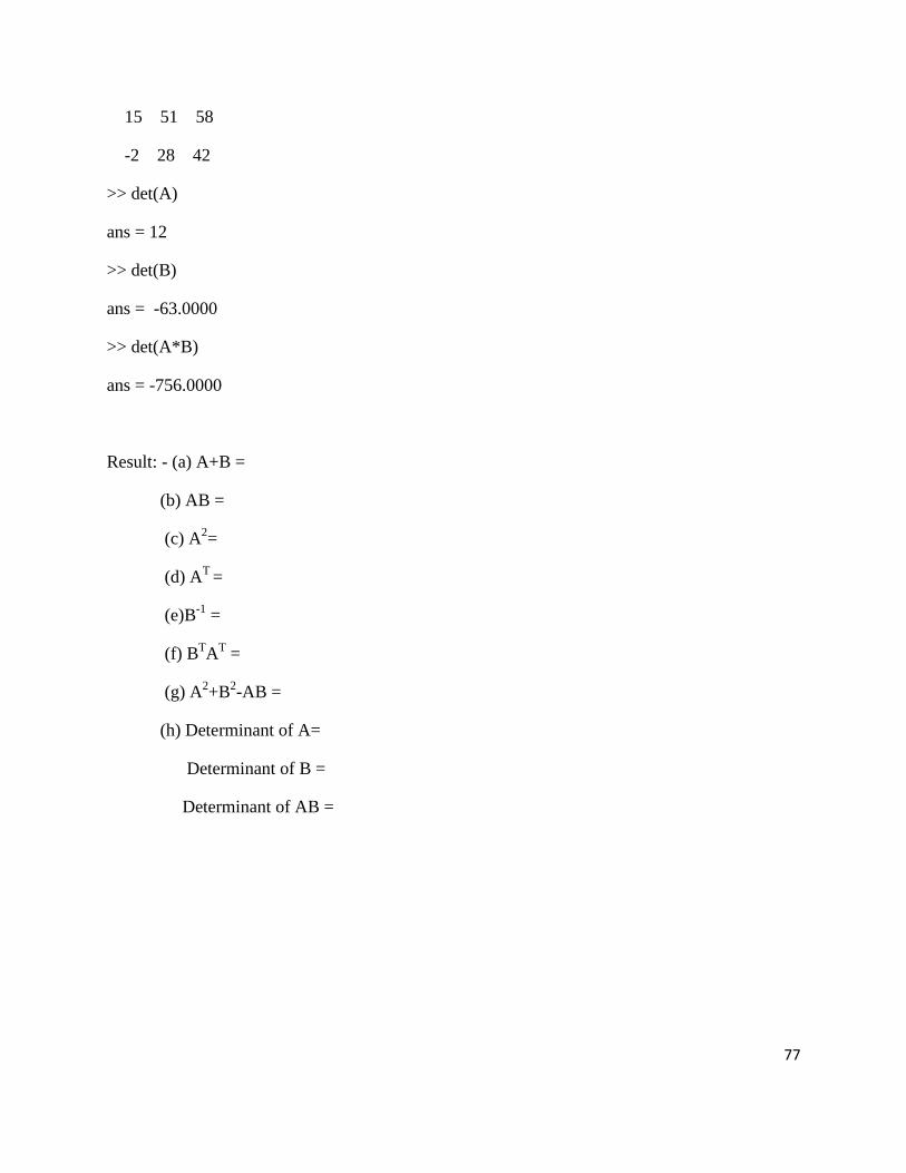
77
15 51 58
-2 28 42
>> det(A)
ans = 12
>> det(B)
ans = -63.0000
>> det(A*B)
ans = -756.0000
Result: - (a) A+B =
(b) AB =
(c) A2=
(d) AT
=
(e)B-1
=
(f) BTA
T =
(g) A2+B
2-AB =
(h) Determinant of A=
Determinant of B =
Determinant of AB =

78
EX.NO.13: DETERMINATION OF EIGEN VALUES AND EIGEN
VECTORS
DATE:
AIM:
To determine the eigenvalues and eigenvectors of A and B using MATLAB
A = and B =
Solution
>> A=[4 2 -3; -1 1 3; 2 5 7]
A =4 2 -3
-1 1 3
2 5 7
>> B=[1 2 3; 8 7 6; 5 3 1]
B =1 2 3
8 7 6
5 3 1
>> eig(A)
ans =0.5949
3.0000
8.4051
>> lamda=eig(A)
lamda = 0.5949
3.0000
79
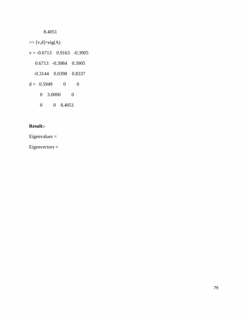
8.4051
>> [v,d]=eig(A)
v = -0.6713 0.9163 -0.3905
0.6713 -0.3984 0.3905
-0.3144 0.0398 0.8337
d = 0.5949 0 0
0 3.0000 0
0 0 8.4051
Result:-
Eigenvalues =
Eigenvectors =
80
EX.NO.14: SOLUTION OF SIMULTANEOUS EQUATIONS
DATE:
AIM:
Solve the following set of equations using MATLAB
x1+2x2+3x3+5x4=21
-2x1+5x2+7x3-9x4=18
5x1+7x2+2x3-5x4=25
-x1+3x2-7x3+7x4=30
Solution
[A][x] = [B]
x =
[x] = [A]-1
B
>> A=[1 2 3 5; -2 5 7 -9; 5 7 2 -5; -1 3 -7 7]
A= 1 2 3 5
-2 5 7 -9
5 7 2 -5
-1 3 -7 7
>> B=[21; 18; 25; 30]
B = 21
18
25
30
81
>> X=inv(A)*B
X = -1.5130
5.9108
0.3762
1.9126
>> check=A*X
check =
21.0000
18.0000
25.0000
30.0000
Result:-
=

82
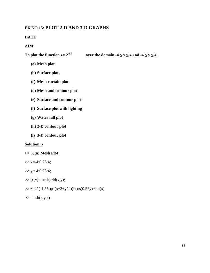
83
EX.NO.15: PLOT 2-D AND 3-D GRAPHS
DATE:
AIM:
To plot the function z= 2-1.5
over the domain -4 ≤ x ≤ 4 and -4 ≤ y ≤ 4.
(a) Mesh plot
(b) Surface plot
(c) Mesh curtain plot
(d) Mesh and contour plot
(e) Surface and contour plot
(f) Surface plot with lighting
(g) Water fall plot
(h) 2-D contour plot
(i) 3-D contour plot
Solution :-
>> %(a) Mesh Plot
>> x=-4:0.25:4;
>> y=-4:0.25:4;
>> [x,y]=meshgrid(x,y);
>> z=2^(-1.5*sqrt(x^2+y^2))*cos(0.5*y)*sin(x);
>> mesh(x,y,z)

84
(b) Surface Plot
(c) Mesh curtain plot

85
>> %(b) Surface Plot
>> x=-4:0.25:4;
>> y=-4:0.25:4;
>> [x,y]=meshgrid(x,y);
>> z=2^(-1.5*sqrt(x^2+y^2))*cos(0.5*y)*sin(x);
>> surf(x,y,z)
>> %(c) Mesh curtain plot
>> x=-4:0.25:4;
>> y=-4:0.25:4;
>> [x,y]=meshgrid(x,y);
>> z=2^(-1.5*sqrt(x^2+y^2))*cos(0.5*y)*sin(x);
>> meshz(x,y,z)
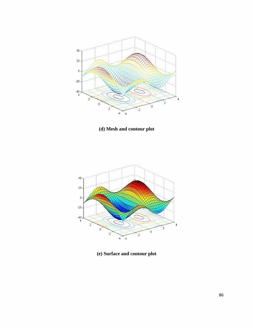
86
(d) Mesh and contour plot
(e) Surface and contour plot
87
>> %(d) Mesh and contour plot
>> x=-4:0.25:4;
>> y=-4:0.25:4;
>> [x,y]=meshgrid(x,y);
>> z=2^(-1.5*sqrt(x^2+y^2))*cos(0.5*y)*sin(x);
>> meshc(x,y,z)
>> %(e) Surface and contour plot
>> x=-4:0.25:4;
>> y=-4:0.25:4;
>> [x,y]=meshgrid(x,y);
>> z=2^(-1.5*sqrt(x^2+y^2))*cos(0.5*y)*sin(x);
>> surfc(x,y,z)

88
(f) Surface plot with lighting
(g) Water fall plot

89
>> %(f) Surface plot with lighting
>> x=-4:0.25:4;
>> y=-4:0.25:4;
>> [x,y]=meshgrid(x,y);
>> z=2^(-1.5*sqrt(x^2+y^2))*cos(0.5*y)*sin(x);
>> surfl(x,y,z)
>> %(g) Water fall plot
>> x=-4:0.25:4;
>> y=-4:0.25:4;
>> [x,y]=meshgrid(x,y);
>> z=2^(-1.5*sqrt(x^2+y^2))*cos(0.5*y)*sin(x);
>> waterfall(x,y,z)

90
(h) 2-D Contour plot
(i) 3-D Contour plot
91
>> %(h) 2-D Contour plot
>> x=-4:0.25:4;
>> y=-4:0.25:4;
>> [x,y]=meshgrid(x,y);
>> z=2^(-1.5*sqrt(x^2+y^2))*cos(0.5*y)*sin(x);
>> contour(x,y,z,15)
>> %(i) 3-D Contour plot
>> x=-4:0.25:4;
>> y=-4:0.25:4;
>> [x,y]=meshgrid(x,y);
>> z=2^(-1.5*sqrt(x^2+y^2))*cos(0.5*y)*sin(x);
>> contour3(x,y,z,15)
Result:-
The following plots were drawn Mesh plot, Surface plot, Mesh curtain plot, Mesh and
contour plot, Surface and contour plot, Surface plot with lighting, Water fall plot, 2-D
contour plot and 3-D contour plot
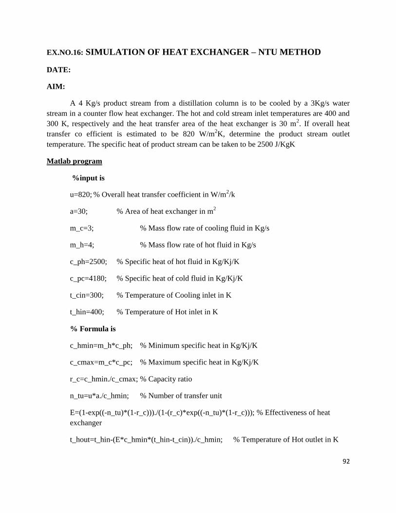
92
EX.NO.16: SIMULATION OF HEAT EXCHANGER – NTU METHOD
DATE:
AIM:
A 4 Kg/s product stream from a distillation column is to be cooled by a 3Kg/s water
stream in a counter flow heat exchanger. The hot and cold stream inlet temperatures are 400 and
300 K, respectively and the heat transfer area of the heat exchanger is 30 m2. If overall heat
transfer co efficient is estimated to be 820 W/m2K, determine the product stream outlet
temperature. The specific heat of product stream can be taken to be 2500 J/KgK
Matlab program
%input is
u=820; % Overall heat transfer coefficient in W/m2/k
a=30; % Area of heat exchanger in m2
m_c=3; % Mass flow rate of cooling fluid in Kg/s
m_h=4; % Mass flow rate of hot fluid in Kg/s
c_ph=2500; % Specific heat of hot fluid in Kg/Kj/K
c_pc=4180; % Specific heat of cold fluid in Kg/Kj/K
t_cin=300; % Temperature of Cooling inlet in K
t_hin=400; % Temperature of Hot inlet in K
% Formula is
c_hmin=m_h*c_ph; % Minimum specific heat in Kg/Kj/K
c_cmax=m_c*c_pc; % Maximum specific heat in Kg/Kj/K
r_c=c_hmin./c_cmax; % Capacity ratio
n_tu=u*a./c_hmin; % Number of transfer unit
E=(1-exp((-n_tu)*(1-r_c)))./(1-(r_c)*exp((-n_tu)*(1-r_c))); % Effectiveness of heat
exchanger
t_hout=t_hin-(E*c_hmin*(t_hin-t_cin))./c_hmin; % Temperature of Hot outlet in K
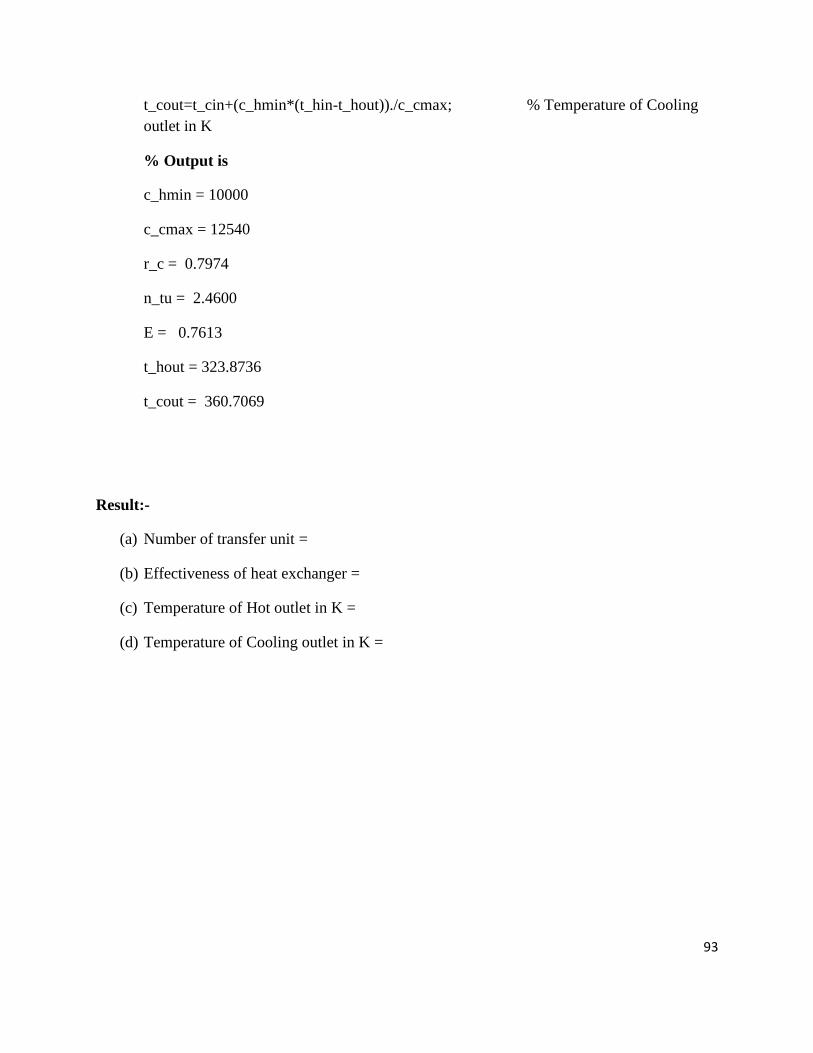
93
t_cout=t_cin+(c_hmin*(t_hin-t_hout))./c_cmax; % Temperature of Cooling
outlet in K
% Output is
c_hmin = 10000
c_cmax = 12540
r_c = 0.7974
n_tu = 2.4600
E = 0.7613
t_hout = 323.8736
t_cout = 360.7069
Result:-
(a) Number of transfer unit =
(b) Effectiveness of heat exchanger =
(c) Temperature of Hot outlet in K =
(d) Temperature of Cooling outlet in K =

94
EX.NO.16: SIMULATION OF HEAT EXCHANGER – NTU METHOD
DATE:
AIM:
The flow rates of hot and cold water streams running through a parallel flow heat
exchanger are 0.2 Kg/s and 0.5 kg/s respectively. The inlet temperatures on the hot and cold
sides are 75oC and 20
oC respectively. The exit temperature of hot water is 45
oC. If the individual
heat transfer coefficients on both sides are 650 W/m2o
C, calculate the area of heat exchanger.
Matlab program
>> %input is
m_h=0.2; % Mass flow rate of cooling fluid in Kg/s
m_c=0.5; %Mass flow rate of cooling fluid in Kg/s
t_hin=75; % Temperature of Hot inlet in K
t_hout=45; %Temperature of Hot outlet in K
t_cin=20; %Temperature of Cooling inlet in K
h_in=650; %heat transfer coefficient inlet in w/m2/oC
h_out=650; % heat transfer coefficient inlet in w/m2/oC
c_ph=4187; % Specific heat of hot fluid in Kg/KJ/oC
c_pc=4187; %Specific heat of cold fluid in Kg/KJ/ oC
%formula is
q=m_h*c_ph*(t_hin-t_hout); % heat transfer in watts
t_cout=t_cin+(m_h*c_ph*(t_hin-t_hout))./(m_c*c_pc);% Temperature of Cooling outlet in oC
l_mtdpf=(t_hin-t_cin)-(t_hout-t_cout)./log((t_hin-t_cin)./(t_hout-t_cout)); %log mean temp. diff.
u=(h_in*h_out)./(h_in+h_out); %Overall heat transfer coefficient in W/m2/k
a=q./(u*l_mtdpf); %area of heat exchanger in m2
% Output is
95
q = 2.5122e+04
t_cout = 32
l_mtdpf = 45.9871
u = 325
a =21.6809
Result:-
(a) heat transfer in watts =
(b) Temperature of Cooling outlet in oC =
(c) LMTDPF =
(d) Overall heat transfer coefficient in W/m2/k =
(e) area of heat exchanger in m2 =