six sigma green belt part 3 - institute of industrial and …1).pdf · 3-1 six sigma green belt...
TRANSCRIPT

3-1
Six Sigma Green Belt
Part 3
Statistics

© 2011 IIE and Aft Systems, Inc. 3-2
Statistics
1. Central Location
1. Mean
2. Median
3. Mode
2. Variability
1. Range
2. Standard Deviation
3. Shape

© 2011 IIE and Aft Systems, Inc. 3-3
Measures of Central Location
The average is the expected value or the balance point
– Mode is the most frequently occurring value
– Median is the middle value
– Arithmetic mean is the total of the individual values divided by the number of individual values
average population theis
average sample theis
x

© 2011 IIE and Aft Systems, Inc. 3-4
Which Mean do you Mean?
• Use the median or the mode if the shape of the distribution is not symmetrical
• Use the arithmetic mean if the shape of the distribution is symmetrical

© 2011 IIE and Aft Systems, Inc. 3-5
Example
Determine the mode, median, and the mean of the following sample:
6,7,7,8,8,8,9,9,9,9,10,10,11,11,12,13

© 2011 IIE and Aft Systems, Inc. 3-6
Example
Calculate the mean of the following samples:
1) 2 3 6 9 1
2) 3 6 4 1 11
3) 2 7 22 0 9
4) -4 8 0 14 0

© 2011 IIE and Aft Systems, Inc. 3-7
Measures of Variability
• The range is the difference between the largest and the smallest values in the sample. The symbol for the range is R.
• The standard deviation is a mathematical measure of the variability of the data about the mean. Its symbol is either s or s.

© 2011 IIE and Aft Systems, Inc. 3-8
Exercise
Calculate the range of the following samples:
1) 2 3 6 9 1
2) 3 6 4 1 11
3) 2 7 22 0 9
4) -4 8 0 14 0
© 2011 IIE and Aft Systems, Inc. 3-9
Calculating Sample Standard
Deviation
Where n is the number of values in the sample

© 2011 IIE and Aft Systems, Inc. 3-10
Standard Deviation Significance
Between plus and minus one standard deviation of the mean, we normally expect to find about 68% of the values
1s 1s
© 2011 IIE and Aft Systems, Inc. 3-11
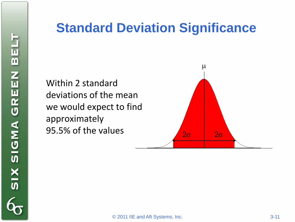
Standard Deviation Significance
Within 2 standard deviations of the mean we would expect to find approximately 95.5% of the values 2s 2s

© 2011 IIE and Aft Systems, Inc. 3-12
Standard Deviation Significance
Within 3 standard deviations of the mean we would expect to find about 99.73% of the values. This is virtually all of the values and represents the expected limits of common cause variation necessary for a stable and predictable process.
3s 3s
© 2011 IIE and Aft Systems, Inc. 3-13
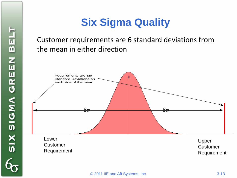
Six Sigma Quality
Customer requirements are 6 standard deviations from the mean in either direction
Requirements are Six
Standard Deviations on
each side of the mean
6s 6s
Lower
Customer
Requirement
Upper
Customer
Requirement
© 2011 IIE and Aft Systems, Inc. 3-14
Grand Average
• The grand average is the process average. It is usually the average of the sample averages. (As long as all of the samples are the same size.)
• It is also the average of all the individuals.
x

© 2011 IIE and Aft Systems, Inc. 3-15
Exercise
Calculate the grand average for the following:
1) 2 3 6 9 1
2) 3 6 4 1 11
3) 2 7 22 0 9
4) -4 8 0 14 0
© 2011 IIE and Aft Systems, Inc. 3-16
Average Range
The average range is the estimate for total process variability. The average range is the average of the sample ranges.
R

© 2011 IIE and Aft Systems, Inc. 3-17
Exercise
Calculate the R bar for the following data:
1) 2 3 6 9 1
2) 3 6 4 1 11
3) 2 7 22 0 9
4) -4 8 0 14 0

© 2011 IIE and Aft Systems, Inc. 3-18
Describing Data
• We describe data to assist with the analyze in six sigma. In order to completely describe data we need to know the following:
– Location
– Spread
– Shape
– Variation Over Time

© 2011 IIE and Aft Systems, Inc. 3-19
Target
Most measures have targets. For example, an organization may promise delivery in 24 hours. That is the target. (In manufacturing that is called the nominal. In service it may be called the customer requirement.)

© 2011 IIE and Aft Systems, Inc. 3-20
Shape
The histogram shows us the shape of the distribution. Many measurements follow the normal or bell shaped curve.

© 2011 IIE and Aft Systems, Inc. 3-21
Shape
• Sometimes the shape is not normal
• We must compare our shape with the expected shape to see if the process is behaving like it always has

© 2011 IIE and Aft Systems, Inc. 3-22
Shape
• We can use the histogram to compare the observed shape with the expected shape
• If the pattern is different from what we expect, then we may not be doing what we always have. We may not be predictable. We may not be stable.