size value and momentum in international stock returns nov 2010
TRANSCRIPT

8/3/2019 Size Value and Momentum in International Stock Returns Nov 2010
http://slidepdf.com/reader/full/size-value-and-momentum-in-international-stock-returns-nov-2010 1/38
First draft: May 2010
This draft: November 2010
Size, Value, and Momentum in International Stock Returns
Eugene F. Fama and Kenneth R. French*
Abstract
In the four regions (North America, Europe, Japan, and Asia Pacific) we examine, there are value
premiums in average stock returns that, except for Japan, decrease with size. Except for Japan, there is
return momentum everywhere, and spreads in average momentum returns also decrease from smaller to
bigger stocks. We test whether empirical asset pricing models capture the value and momentum patterns
in international average returns and whether asset pricing seems to be integrated across the four regions.
Integrated pricing across regions does not get strong support in our tests, but local models for three
regions (North America, Europe, and Japan) provide passable stories for local average returns, which is
consistent with integrated pricing within these regions.
* Booth School of Business, University of Chicago (Fama) and Amos Tuck School of Business, Dartmouth College
(French). We thank Stanley Black and Tu Nguyen of Dimensional Fund Advisors for painstaking work in
assembling the data for this paper.

8/3/2019 Size Value and Momentum in International Stock Returns Nov 2010
http://slidepdf.com/reader/full/size-value-and-momentum-in-international-stock-returns-nov-2010 2/38
2
Banz (1981) finds that stocks with lower market capitalization (small stocks) tend to have higher
average returns. There is also evidence that value stocks, that is, stocks with high ratios of a fundamental
like book value or cash flow to price, have higher average returns than growth stocks, which have low
ratios of fundamentals to price (Rosenberg, Reid, and Lanstein (1985), DeBondt and Thaler (1985), Fama
and French (1992), Lakonishok, Shleifer, and Vishny (1994)). U.S. stock returns also exhibit momentum:
stocks that have done well over the past year tend to continue to do well for a few months (Jegadeesh and
Titman (1993)). The value premium (higher average returns of value stocks relative to growth stocks)
and momentum are also observed in international stock returns (Chan, Hamao, and Lakonishok (1991),
Fama and French (1998), Rouwenhurst (1998), Asness, Moskowitz, and Pedersen (2009)).
Fama and French (1993) propose a three-factor model to capture the patterns in U.S. average
returns associated with size and value versus growth,
(1) Ri(t) – RF(t) = ai + bi[RM(t) – RF(t)] + siSMB(t) + hiHML(t) + ei(t).
In this regression, Ri(t) is the return on asset i for month t, RF(t) is the riskfree rate, RM(t) is the
market return, SMB(t) is the difference between the returns on diversified portfolios of small stocks and
big stocks, and HML(t) is the difference between the returns on diversified portfolios of high book-to-
market (value) stocks and low book-to-market (growth) stocks. In an attempt to also capture momentum
returns, Carhart (1997) proposes a four-factor model for U.S. returns,
(2) Ri(t) – RF(t) = ai + bi[RM(t) – RF(t)] + siSMB(t) + hiHML(t) + wiWML(t) + ei(t),
which is (1) enhanced with a momentum return, WML(t), the difference between the month t returns on
diversified portfolios of the winners and losers of the past year.
Regressions (1) and (2) are commonly used in applications, most notably to evaluate portfolio
performance (Carhart (1997), Kosowski et al. (2006), Fama and French (2010)). In the initial paper on
the three-factor model, however, Fama and French (1993) find that, although it captures the size and
value patterns in post-1962 U.S. average returns better than the CAPM, there are holes in the model’s

8/3/2019 Size Value and Momentum in International Stock Returns Nov 2010
http://slidepdf.com/reader/full/size-value-and-momentum-in-international-stock-returns-nov-2010 3/38
3
explanation of average returns. There is a large literature on momentum, but we know of no evidence on
how well the Carhart four-factor model captures momentum patterns in average returns.
This paper examines international stock returns, with two goals. The first is to detail the size,
value, and momentum patterns in average returns for major developed markets. Our main contribution is
evidence for different size groups. Most prior work on international returns focuses on large stocks. Our
sample covers all size groups, and tiny stocks (microcaps) produce some of the most interesting results.
Our second goal is to examine how well (1) and (2), and an extension of them, capture average returns for
portfolios formed on size and value or size and momentum. We examine local versions of the models in
which the explanatory returns (factors) and the returns to be explained are from the same region. To
develop perspective on whether asset pricing is integrated across regions, we also examine models that
use global factors to explain global and regional returns.
There is a literature on integrated international asset pricing, ably reviewed by Karolyi and Stulz
(2003). The papers closest to ours are Griffin (2002) and Hou, Karolyi, and Kho (2009). We add to their
work in many ways. For example, Griffin (2002) examines whether country-specific or aggregate
versions of (1) better explain returns on portfolios and individual stocks in the U.S., the U.K., Canada,
and Japan. We use 23 countries. Hou, Karolyi, and Kho (2009) do not examine how value premiums and
momentum returns differ across size groups and whether the size patterns in average value premiums and
momentum returns are captured by local and international asset pricing models – our main tasks.
Section I discusses the motivation for the asset pricing tests. Section II describes the data and
variables. Section III presents summary statistics for returns. Sections IV and V turn to tests of asset
pricing models. Section VI summarizes the results and presents conclusions.
I. Motivation
Regressions (1) and (2) are motivated by observed patterns in returns. They are examples of
empirical asset-pricing models; that is, they try to capture the cross-section of expected returns without
specifying the underlying economic model that governs asset pricing. When we propose regressions like

8/3/2019 Size Value and Momentum in International Stock Returns Nov 2010
http://slidepdf.com/reader/full/size-value-and-momentum-in-international-stock-returns-nov-2010 4/38
4
(1) or (2) as empirically motivated asset-pricing models, the hypothesis is that the regression slopes for
the explanatory returns capture the cross-section of expected returns, so the true intercepts are zero for all
left-hand-side (LHS) assets. This in turn implies that the portfolios on the right hand side (RHS) span the
ex ante mean-variance-efficient (MVE) tangency portfolio that can be created from all assets (Huberman
and Kandel (1987)). If we find a set of explanatory portfolios that spans the MVE tangency portfolio, we
capture the cross-section of expected returns, whatever the underlying model generating asset prices.
That the true MVE tangency portfolio can be used to describe expected returns on all assets is, on
the most general level, an algebraic result (e.g., Roll (1997)). By way of economic motivation, the MVE
tangency portfolio has a role in all versions of Merton’s (1973) ICAPM, including the CAPM of Sharpe
(1964) and Lintner (1965). Specifically, the MVE tangency portfolio is always one of the “multifactor
efficient” portfolios relevant for choice by investors (Fama (1996)). Thus, in an ICAPM world, using the
tangency portfolio to describe expected returns has economic content.
Empirical asset pricing is empty if the search for the MVE tangency portfolio is unrestricted.
There is, after all, a tangency portfolio for any set of assets. To make empirical asset pricing interesting,
restrictions must be imposed. The restrictions focus on parsimony. Models like (1) and (2) ask whether a
small set of RHS portfolios, directed at patterns in average returns observed over long periods, capture the
MVE tangency portfolio implied by the expected returns and return covariances of assets.
We study international returns, and the goal is to examine two related issues; (i) whether
parsimonious empirical asset pricing models capture the value and momentum patterns in international
average returns, and (ii) the extent to which asset pricing is integrated across markets. The task faces bad
model problems. Any model is an approximation to the pricing process, and so likely to be rejected in
tests that have power. For example, the general form of the model may be incorrect; that is, there may be
no version of the RHS explanatory returns that spans the MVE tangency portfolio of interest.
Alternatively, the bad model problem may be the absence of integrated asset pricing in the region
covered by the RHS returns. Thus, suppose we have the correct asset pricing model; that is, applied to the
8/3/2019 Size Value and Momentum in International Stock Returns Nov 2010
http://slidepdf.com/reader/full/size-value-and-momentum-in-international-stock-returns-nov-2010 5/38
5
broadest region in which asset pricing is integrated, the model’s RHS portfolios span the MVE tangency
portfolio for the region. Then if we regress the excess returns on any assets from the integrated pricing
region on the model’s RHS returns for the region, we get intercepts that are indistinguishable from zero.
But we expect intercept tests to reject if we use explanatory returns for narrower or broader regions.
For example, suppose the true model generating asset prices is the CAPM and pricing is globally
integrated. Then βs with respect to the global market portfolio explain expected returns on all assets, but
local versions of the CAPM should not work. For example, βs with respect to the U.S. market portfolio
should not explain expected returns on all U.S. assets. On the other hand, if markets are not globally
integrated, the global CAPM should fail even if a local CAPM prices assets in each market.
We shall see that power is often a problem in tests of these predictions. We sometimes have too
little and sometimes we have too much. When the dependent and explanatory returns in our asset pricing
regressions are for the same region (local or global), the tests typically have power because the regression
fits are tight (R2 is high). As a result, we shall see some formal rejections of models that in economic
terms seem to be reasonable approximations. On the other hand, when the RHS portfolios are global and
the LHS assets are local (that is, restricted to one of the four regions), the regressions fit less tightly and
power is often a problem. Perhaps as a result, we shall see tests in which we fail to reject global models
that seem far off target in explaining local average returns.
The results from the tests for global integration are at best mixed, which opens the door for local
models. Moreover, we shall see that in tests to explain local LHS returns, local RHS returns produce
tighter fits and more precise parameter estimates than global RHS returns. Thus, even if global models
produced clean evidence of integrated pricing, local models may be attractive in applications to explain
local LHS returns as long as the local RHS portfolios produce a passable approximation to the MVE
tangency portfolio for local assets. For example, even with integrated global pricing, a passable local
model that uses RHS returns for North America may be attractive for evaluating the performance of a

8/3/2019 Size Value and Momentum in International Stock Returns Nov 2010
http://slidepdf.com/reader/full/size-value-and-momentum-in-international-stock-returns-nov-2010 6/38
6
mutual fund that holds only North American stocks because the local model provides more precise alpha
estimates than the global model.
We examine local asset pricing models for each of our four regions. The tests of local models
typically have power. Nevertheless, the local models perform rather well in capturing the returns on local
portfolios. We take this to be good news for potential applications of such models.
II. Data and Variables
Our international stock returns and accounting data are primarily from Bloomberg. The sample
period for all 23 countries we examine is November 1989 to September 2010. There are other sources for
international returns on big stocks prior to 1989, but our goal is to extend the international evidence to
small stocks. The cost is a rather short 20+ year sample period. All our returns are in U.S. dollars and
monthly excess returns are returns in excess of the one-month U.S. Treasury bill rate (from CRSP).
To ensure that we have plenty of stocks in each of the LHS portfolios, we combine our 23
developed markets into four regions: (i) North America (NA), which includes the United States and
Canada; (ii) Japan; (iii) Asia Pacific, including Australia, New Zealand, Hong Kong, and Singapore (but
not Japan); and (iv) Europe, including Austria, Belgium, Denmark, Finland, France, Germany, Greece,
Ireland, Italy, the Netherlands, Norway, Portugal, Spain, Sweden, Switzerland, and the United Kingdom.
We also examine global portfolios that combine the four regions. On average, North America, Europe,
Japan, and Asia Pacific account for 47.3%, 30.0%, 18.4%, and 4.3% of global market capitalization.
Parsimony in the choice of regions is important in the power of our tests, but we also want
regions in which market integration is a reasonable assumption. It seems reasonable to assume that the
U.S. and Canada are close to one market for goods and securities during our sample period. The
countries of Europe are almost all members of the European Union, and those that are not formal
members (e.g., Switzerland) participate in most of the EU’s open market provisions. In terms of countries
with mutually open markets, the (rather small) Asia Pacific region is most questionable, and we shall see
that it is a problem in some of our tests.
8/3/2019 Size Value and Momentum in International Stock Returns Nov 2010
http://slidepdf.com/reader/full/size-value-and-momentum-in-international-stock-returns-nov-2010 7/38
7
In each region, we sort stocks on size (market cap) and momentum, and on size and the ratio of
book equity to market equity (B/M). In our previous work on U.S. stocks (Fama and French (1993)) we
use NYSE breakpoints for size and B/M, to avoid sorts that are dominated by the plentiful but less
important tiny Amex and NASDAQ stocks. For the same reason, in our current tests we use B/M and
momentum breakpoints based on large stocks and size breakpoints that are percents of aggregate market
cap chosen to avoid undo weight on tiny stocks.
Specifically, the explanatory returns in our asset pricing tests are for portfolios constructed from
2x3 sorts on size and B/M or size and momentum. At the end of June of each year t we sort the stocks in
a region on market cap and B/M. Big stocks are those in the top 90% of market cap for the region, and
small stocks are those in the bottom 10%. (For North America, 90% of market cap corresponds roughly
to the NYSE median, used to define small and big stocks in Fama and French (1993).) The B/M
breakpoints in the 2x3 sorts for the four regions are the 30th
and 70th
percentiles of B/M for the big stocks
of a region, where, as in Fama and French (1993), book value is for the fiscal year ending in calendar year
t-1 and market cap is for the end of December of calendar year t-1. The global portfolios use global size
breaks. Because we worry about differences in accounting rules across the four regions, however, we use
each region’s B/M breakpoints to allocate its stocks to the global portfolios. Similarly, we use regional
momentum breakpoints (described below) when forming global size-momentum portfolios.
For each region, the intersection of the independent 2x3 sorts on size and B/M produces six
portfolios, SG, SN, SV, BG, BN, and BV, where S and B indicate small or big and G, N, and V indicate
growth, neutral, and value (bottom 30%, middle 40%, and top 30% of B/M) respectively. We compute
monthly value-weight returns for each portfolio from July of year t to June of t+1. The size factor, SMB,
for a region is the equal-weight average of the returns on the three small stock portfolios from the 2x3
size-B/M sorts for the region minus the average of the returns on the three big stock portfolios. For each
region, we construct value – growth returns for small and big stocks, HML_S = SV – SG and HML_B =
BV – BG, and HML is the equal-weight average of HML_S and HML_B.

8/3/2019 Size Value and Momentum in International Stock Returns Nov 2010
http://slidepdf.com/reader/full/size-value-and-momentum-in-international-stock-returns-nov-2010 8/38
8
As in Fama and French (1993), at the end of June of each year we also construct 25 size-B/M
portfolios for each region, to be used as LHS assets in asset pricing regressions. The size breakpoints for
a region are the 3rd
, 7th, 13
th, and 25
thpercentiles of the region’s aggregate market capitalization. (These
correspond roughly to the average market caps for the NYSE quintile breakpoints for size used in Fama
and French (1993).) The B/M breakpoints in the 5x5 sorts follow the same rules as the 2x3 sorts, except
we use the separate quintile B/M breakpoints (rather than 30-40-30 splits) for big (top 90% of market cap)
stocks in each region to allocate the region’s big and small stocks. The 25 value-weight size-B/M
portfolios for the region are the intersections of the independent 5x5 size and B/M sorts.
We do 2x3 and 5x5 sorts on size and momentum using the same breakpoint conventions as the
size-B/M sorts, except that the size-momentum portfolios are formed monthly and the lagged momentum
return takes the place of B/M. For portfolios formed at the end of month t, the lagged momentum return
is a stock’s average monthly return for t-11 to t-1. (Skipping the sort month is standard in momentum
tests.) The intersection of the independent 2x3 sorts on size and momentum produces six value-weight
portfolios, SL, SN, SW, BL, BN, and BW, where S and B indicate small and big, and L, N, and W
indicate losers, neutral, and winners (bottom 30%, middle 40%, and top 30% of lagged momentum). In
the 2x3 sorts we construct winner – loser returns for small and big stocks, WML_S = SW – SL and
WML_B = BW – BL, and WML is the equal-weight average of WML_S and WML_B. The intersections
of the independent 5x5 size and momentum sorts for a region produce 25 value-weight portfolios, to be
used as LHS assets in asset pricing regressions. The first momentum sort absorbs a year of data, so the
sample period for all tests is November 1990 through September 2010 (henceforth 1991-2010).
III. Summary Statistics
We begin by examining summary statistics for the RHS explanatory returns in our asset pricing
regressions. We then turn to the 25 portfolios formed on size and B/M, and the 25 size-momentum
portfolios that are the LHS assets in the regressions.

8/3/2019 Size Value and Momentum in International Stock Returns Nov 2010
http://slidepdf.com/reader/full/size-value-and-momentum-in-international-stock-returns-nov-2010 9/38
9
A. Explanatory Returns
Equity premiums for 1991-2010 (the average differences between monthly value-weight market
returns and the one-month U.S. Treasury bill rate) are large in three of the four regions, ranging from
0.52% per month in Europe to 0.86% in Asia Pacific. Japan is the exception, with a negative premium of
-0.15% per month. As usual, the estimates of equity premiums are imprecise. The equity premiums for
our sample period of 20+ years are above the traditional two-standard-error bound in only two of the four
regions, Asia Pacific and North America. The global premium, a respectable 0.39% per month despite
Japan’s poor return, is 1.37 standard errors from zero.
There is no size premium in any region during our sample period. Average SMB returns are of
random sign and all are close to zero. In contrast, there are value premiums everywhere. Average HML
returns for the four basic regions range from 0.35% per month (t = 1.51) for North America to 0.76% (t =
3.51) for Asia Pacific. Echoing Loughran’s (1995) results for the U.S., value premiums are larger for
small stocks. The exception is Japan, where the value premium is similar for small and big stocks, 0.43%
(t = 2.13) and 0.47% per month (t = 1.90). The average global HML return is 0.46% per month (t = 2.83),
but the premium for small stocks 0.68% (t = 3.71) is much larger than the premium for big stocks, 0.24%
(t = 1.34), and the difference, 0.44% per month, is 2.79 standard errors from zero.
The evidence that international value premiums are larger for small stocks seems contrary to the
results in Fama and French (2006). The sample of the earlier paper is, however, thin on small stocks.
The more complete current sample suggests that larger value premiums for small stocks are typical.
There are similar size patterns in momentum returns that are common to all our regions except
Japan. Like Asness, Moskowitz, and Pedersen (2009), we find strong momentum returns everywhere,
except Japan. Average WML returns for the other three regions range from 0.67% per month (t = 1.97)
for North America to 0.91% (t = 3.29) for Europe. Echoing previous results for the U.S. (Hong, Stein,
and Lim (2000)), average WML returns for all regions except Japan are larger for small stocks. The
global results are a good summary. The average global WML return is 0.61% per month (t = 2.24), the

8/3/2019 Size Value and Momentum in International Stock Returns Nov 2010
http://slidepdf.com/reader/full/size-value-and-momentum-in-international-stock-returns-nov-2010 10/38
10
result of 0.81% (t = 3.01) for small stocks and 0.42% (t = 1.37) for big stocks. The differences between
average WML returns for small and big stocks exceed two standard errors for all regions, except Japan.
For Japan, average WML returns are close to zero for small and big stocks.
B. Excess Returns for the 25 Size-B/M and the 25 Size-Momentum Portfolios
For a sample period preceding that used here, Fama and French (1993) find that the low returns of
small U.S. growth stocks are a problem in their asset pricing tests. Part A of Table 2 shows that for our
new 1991-2010 sample, low returns for small growth stocks are common to all regions except Japan.
Japan aside, for extreme growth stocks (the left column of the 5x5 size-B/M matrices), the small stock
portfolios have lower average returns than the big stock portfolios – a reverse size effect.
Japan aside, there is a standard size effect in the right column of the 5x5 size-B/M matrices; small
extreme value (high B/M) stocks have higher average returns than big extreme value stocks. For every
region including Japan, there are value premiums in all size groups; average returns increase from left to
right in every row of the size-B/M matrices. But lower average returns of small stocks in the left column
of the matrices for North America, Europe, and Asia Pacific combine with a typical size effect in the right
column to produce larger value premiums for small stocks, especially microcaps. This common size
pattern in value premiums is a major factor in our later rejections of the three-factor model (1).
Part B of Table 2 shows matrices of average excess returns for the 25 size-momentum portfolios
of our four regions. For Japan there is no hint of momentum in any size group. For all other regions
there are momentum returns in all size groups; average returns increase from left ( last year’s losers) to
right (winners) in all rows of the 5x5 matrices. There is no consistent relation between average return and
size in the first two columns of the matrices; losers lose similarly in all size groups. A typical size effect
(higher average returns for small stocks) shows up in the fourth column of the matrices, and it is more
evident in the fifth column. Thus, last year’s winners show positive momentum returns in all size groups,
but the persistence is stronger for small stocks, especially microcaps. The size pattern in momentum
returns is a major factor in our eventual rejections of the four-factor model (2).

8/3/2019 Size Value and Momentum in International Stock Returns Nov 2010
http://slidepdf.com/reader/full/size-value-and-momentum-in-international-stock-returns-nov-2010 11/38
11
IV. Regressions for Size-B/M Portfolios
Tables 3 and 4 summarize regressions to explain excess returns on the portfolios from the 5x5
sorts on size and B/M. Table 3 shows the F-test of Gibbons, Ross, and Shanken (GRS, 1989) and other
summary statistics for the regression intercepts for the four models we consider. Table 4 shows matrices
of the intercepts and their t-statistics for selected models. (Detailed regression results are available on
request.) For the global LHS portfolios we use only global explanatory returns. For the four regions, we
examine results for local and global explanatory returns.
A. Global Models for Global Size-B/M Portfolio Returns
The regressions in which global portfolios provide both dependent and explanatory returns
illustrate many of the asset pricing problems we encounter. Because the global LHS size-B/M portfolios
are quite diversified, they identify the problems with precision. Moreover, if we use the correct asset
pricing model, the tests to explain global returns with global factors provide evidence on whether asset
pricing is integrated across our four developed regions. The tests that use global factors to explain returns
for the four regions then give details about sources of success and failure.
The global CAPM fares poorly in our tests. The GRS statistic for the CAPM regressions, 4.54 in
Table 3, is in the distant right tail of the relevant F-distribution, and the CAPM intercepts (Table 4) are
always negative for extreme growth portfolios and positive for extreme value portfolios. The CAPM fails
because market betas for the 25 global size-B/M portfolios (not shown) are, if anything, higher for growth
than for value portfolios, the reverse of what is needed to explain the value premium in global returns.
Switching to the three-factor model (1) improves the description of average returns on the global
portfolios; the GRS statistic falls to 4.02 and the average absolute intercept falls from 0.21% to 0.14%.
Nevertheless, the GRS statistic is far above the 99.9% threshold of 2.26, and we confidently reject the
global three-factor model. The rejection is due in part to tight regression fits. Adding the global SMB
and HML returns raises the average R2
from 0.81 for the CAPM to 0.95 for the three-factor model, and
the average standard error of the intercepts falls by half, from 0.14% to 0.07%. But there are also three-

8/3/2019 Size Value and Momentum in International Stock Returns Nov 2010
http://slidepdf.com/reader/full/size-value-and-momentum-in-international-stock-returns-nov-2010 12/38
12
factor pricing problems. The global model leaves a value pattern in the intercepts for global microcaps
(first row of the intercept matrix in Table 4), and it creates a reverse value pattern (positive intercepts for
growth portfolios and negative for value portfolios) among megacaps (the last row). There is a simple
story. Global value-growth spreads in average returns are larger for small stocks, especially microcaps
(Table 2), but the spreads in three-factor HML slopes (not shown) are not wider for small stocks. Similar
three-factor problems are observed for other regions where value premiums are larger for small stocks.
The global version of Carhart’s (1997) four -factor model (2), which adds the global momentum
return WML to the explanatory returns of the three-factor model (1), lowers the GRS statistic, from 4.02
for the three-factor model to 3.60, and the average absolute intercept falls from 0.14 to 0.12. But the four-
factor model is still rejected, and its intercepts (Table 4) are similar to those from the three-factor model.
Like the three-factor model (1), the four-factor model (2) leaves a value pattern in the intercepts
for microcaps and it creates a reverse value pattern among megacaps. In our later tests to explain the
returns on portfolios formed on size and momentum, the more extreme momentum returns of smaller
stocks, especially microcaps, lead to similar problems (a momentum pattern in the intercepts for
microcaps and a reverse momentum pattern among megacaps) in the estimates of (2). Our response to
these problems is to estimate a six-factor model that uses HML_S, HML_B, WML_S, and WML_B, the
small and big components of HML and WML, as separate explanatory returns,
(3) Ri(t) – RF(t) = ai + bi[RM(t) – RF(t)] + siSMB(t)
+ hsiHML_S(t) + hbiHML_B(t) + wsiWML_S(t) + wbiWML_B(t) + ei(t).
Regression (3) is overkill for explaining size-B/M returns; splitting WML into its small and big
components doesn’t add much. Likewise, s plitting HML into its small and big components doesn’t add
much in the later tests on size-momentum returns. We focus on (3) to have a single model that potentially
provides a unified story for value and momentum returns.
Data dredging is a concern in empirically motivated models like (1) and (2) that are directed at
capturing observed patterns in average returns, and the concern is more serious when we split HML and
8/3/2019 Size Value and Momentum in International Stock Returns Nov 2010
http://slidepdf.com/reader/full/size-value-and-momentum-in-international-stock-returns-nov-2010 13/38
13
WML into small and big components in response to rejections of (1) and (2). We do not want the tests to
degenerate into a search for the ex post MVE tangency portfolio implied by sample-specific patterns in
average returns. Aware of this problem, we offer a justification for (3). Our goal is to capture the ex ante
MVE tangency portfolio implied by the patterns in expected returns. Larger value and momentum
premiums for small stocks are common to all our regions except Japan. If the value and momentum
patterns in expected returns are in fact different for small and big stocks, (1) and (2) may have bad model
problems that are cured in a parsimonious way by (3). At a minimum, estimates of (3) provide
diagnostics that help us understand the shortcomings of (1) and (2).
The six-factor model (3) improves the explanation of returns on the 25 global size-B/M
portfolios. The GRS statistic falls from 3.60 for the four-factor model to 2.61, and the average absolute
six-factor intercept is a respectable 0.11%. But in part due to the tight fit of the six-factor regressions –
the average R2
is 0.96 and the average standard error of the intercepts is 0.07% – the GRS test rejects with
confidence. The matrix of intercepts (Table 4) provides perspective. Microcaps are the global six-factor
model’s big challenge. Though weaker than the pattern left by the four-factor model, a value pattern
remains in the six-factor intercepts for microcaps, with estimates of -0.17% for microcap growth and
0.23% for microcap value. The model has almost no problems with in the three largest size quintiles; the
absolute intercepts for all but one of these 15 portfolios are 0.15% or less. The intercepts for four of the
five portfolios in the second (small) quintile also fall in this band.
The systematic intercept problems of the six-factor model (3) in the tests on global returns seem
limited to microcaps. It is possible that for global size-B/M portfolios, (3) is a passable model for the four
largest size quintiles, asset pricing is globally integrated for stocks in the four largest size quintiles, and
the formal rejection of (3) is due either to the absence of integrated global pricing for microcaps or other
bad model problems exposed by microcaps. As suggestive evidence, Table 3 summarizes tests on the
intercepts from (3) for the global size-B/M portfolios when the microcap (first) row of the intercept
matrix is deleted. Dropping microcaps causes the GRS statistic to fall from 2.61 to 2.34, which still

8/3/2019 Size Value and Momentum in International Stock Returns Nov 2010
http://slidepdf.com/reader/full/size-value-and-momentum-in-international-stock-returns-nov-2010 14/38
14
rejects – even if we ignore the selection bias created by omitting the quintile with the biggest problems.
The tests, however, have substantial power (average R2 is 0.96), and microcaps aside, the performance of
the six-factor model seems acceptable. For example, without microcaps the average absolute intercept in
(3) is 0.09, among the lowest in Table 3.
More interesting, without microcaps the global four-factor model performs as well as the six-
factor model. The GRS statistic, 2.25, and the average absolute intercept, 0.09, just about match the no-
microcap values for the six-factor model, 2.34 and 0.09. These results suggest that, microcaps aside,
integrated global pricing and the four-factor model are a passable story for global size-B/M portfolio
returns – an attractive conclusion, given the data dredging concerns raised by the six-factor model.
It is possible that global LHS portfolios, which mix assets from our four basic regions, conceal
asset pricing problems. For example, the expected returns of the assets of a region (e.g., North America)
may not be captured well by global RHS portfolios, but this information may be buried in tests that use
global LHS portfolios. To check this possibility, we turn now to regressions that use global RHS returns
to explain the returns on LHS portfolios for each of the four basic regions.
B. Global Models for Regional Size-B/M Portfolio Returns
When the tests include microcaps, the GRS statistic (Table 3) cleanly rejects the global versions
of the CAPM, the three-factor model (1), and the four-factor model (2) for the size-B/M portfolio returns
of North America, Europe, and Asia Pacific. The six-factor model (3) fares better, producing a strong
rejection only in the Asia Pacific tests, and marginal rejections for North America and Europe. Again,
microcaps are a problem. When microcaps are dropped, the GRS statistics improve and, if we continue to
ignore the selection bias, only the Asia Pacific tests clearly reject the global six-factor model. Once
again, with microcaps out, the six-factor model is not systematically better than the four-factor model on
the GRS test, and without microcaps the average absolute intercepts are smaller for the four-factor model.
Thus, the tests on regional LHS size-B/M returns seem roughly consistent with the earlier conclusion that,

8/3/2019 Size Value and Momentum in International Stock Returns Nov 2010
http://slidepdf.com/reader/full/size-value-and-momentum-in-international-stock-returns-nov-2010 15/38
15
microcaps aside, integrated four-factor global pricing is a reasonable approximation for size-B/M
portfolio returns.
There are, however, power problems in the tests to explain regional size-B/M returns with global
factors. Japan is the extreme case. Judged on the GRS test, the four global models pass easily when
asked to explain Japanese size-B/M portfolio returns. The four GRS statistics (Table 3) are safely below
1.41, the 90% percentile of the relevant F-distribution. But the power of the tests is low. Average R2
ranges from 0.28 for the CAPM regressions to 0.42 for the six-factor model, and the standard error of the
intercepts averages 0.38% or higher. Moreover, the intercepts (not shown) in the regressions for all
Japanese portfolios and all global models are negative, and the average intercepts (Table 3) are strongly
negative, from -0.49% per month to a huge -1.02%. Thus, in economic terms, the global models fail
badly for Japan. The problem traces to low average excess returns on the 25 Japanese size-B/M portfolios
(Table 2) combined with slopes close to 1.0 (not shown) for the global market excess return, which has a
large positive average value. As a result, average returns on the Japanese size-B/M portfolios are far
lower than predicted by the global models. We can’t reject global CAPM, three-factor, four-factor, or
six-factor pricing for Japan, but we can’t imagine an application in which it is sensible to apply the global
models to Japanese returns.
Global models also have problems in the regressions to explain size-B/M returns for other
regions. With global explanatory returns, the average R2 values are lowest for Japan, but they are also
low for Asia Pacific (around 0.55), and for North America and Europe (around 0.75, versus 0.95 in the
regressions to explain the global size-B/M portfolio returns). With global explanatory returns, the
average standard errors of the intercepts for Asia Pacific size-B/M portfolios (around 0.35) are similar to
the averages for Japan. The averages for the size-B/M portfolios of North America and Europe are lower
(around 0.20), but still large. Finally, with global explanatory returns, there is an average intercept
problem in the regressions for North America like that in the Japan tests, but of opposite sign. The NA
intercepts are systematically positive and large (around 0.40), and as in Japan, the extreme NA intercepts

8/3/2019 Size Value and Momentum in International Stock Returns Nov 2010
http://slidepdf.com/reader/full/size-value-and-momentum-in-international-stock-returns-nov-2010 16/38
16
are common to all size groups, not just microcaps . Again, we can’t imagine an application in which it is
sensible to apply global models to NA returns.
Extreme average intercepts in the estimates of global models on the size-B/M portfolio returns of
Japan and North America suggest that differences in the level of average returns in the four regions are a
problem for the global models. As a check, we use the global models to explain the market portfolio
returns of the regions. Despite poor regression fits (the average R2
is 0.68) the GRS test (Table 5) rejects
the global CAPM for the market returns of the four regions at the 90% level. The GRS test comes close
to rejecting the global three-, four-, and six-factor models for regional market returns at the 95% level.
Once again, the intercepts for the North America market return are large and positive (0.24% to 0.34%) in
the four global models in Table 5, and the intercepts for Japan are large and negative (-0.51% to -0.89%).
Solnik (1974), Harvey (1991), and Fama and French (1998) fail to reject the global CAPM as a model for
country market returns. Our stronger evidence against global models for regional market portfolio returns
may be specific to our sample period, but enhanced power is also a possibility. Previous papers typically
use LHS market portfolios for many countries. In multiple comparisons tests like GRS, more LHS
portfolios can imply less power. Collapsing countries into four regions, with a presumption of integrated
pricing in each region, reduces the power loss.
In short, poor regression fits and large intercepts suggest that global models do not do well when
asked to explain the returns on regional size-B/M portfolios. We see next that local (regional) models are
better for that task.
C. Local Models for Regional Size-B/M Portfolio Returns
The GRS statistic (Table 3) testing whether the Japanese market, SMB, and HML returns capture
the average returns for the 25 Japanese size-B/M portfolios, 0.71, is below the median of the relevant F-
distribution, there are no notable patterns in the matrix of three-factor regression intercepts (Table 4), and
the intercepts are almost all economically and statistically close to zero.
8/3/2019 Size Value and Momentum in International Stock Returns Nov 2010
http://slidepdf.com/reader/full/size-value-and-momentum-in-international-stock-returns-nov-2010 17/38
17
The GRS test suggests that the local CAPM also works in Japan. This failure to reject, however,
is probably due to low power. The average R2 from the CAPM regressions is only 0.78, the average
standard error of the intercepts is 0.22%, the average absolute intercept is 0.17%, and the CAPM leaves a
strong value pattern in the (unreported) intercepts for all five size groups. Adding the three-factor
model’s SMB and HML returns pushes the average R2 up to 0.93, shrinks the average standard error of
the intercepts to 0.12%, and lowers the average absolute intercept to 0.10%. The local four- and six-
factor models do not improve the explanation of the Japanese size-B/M average portfolio returns provided
by the local three-factor model. This is not surprising since Japan is the only region where there is no
momentum and there is no size pattern in value premiums (Table 2).
Judged by GRS statistics, the local six-factor model is the choice for returns on the 25 European
size-B/M portfolios. The GRS test (Table 3) says that the European version of the CAPM does not
capture the cross-section of average returns for the region’s 25 size -B/M portfolios, and there is a value
pattern in the (unreported) CAPM intercepts. The European three-factor model does better, but the
regressions leave a value pattern in the intercepts for microcaps, and they create a reverse value pattern
for megacaps. The added flexibility of the six-factor model allows it to absorb these patterns in the
intercepts. There are no apparent patterns in the six-factor intercepts and the average absolute intercept is
only 0.10% per month. As a result, the GRS statistic for the European six-factor model is only 1.33.
Despite the six-factor model’s GRS victory, one might argue that for applications, the average
absolute intercept is a better metric. On this score, the six-factor model is no better than the three-factor
model in Europe; the average absolute intercept is 0.09 for both (and for the local four-factor model). The
six-factor model absorbs the microcap and megacap patterns in the three-factor intercepts, but it pushes
other intercepts away from zero (Table 4). The European six-factor model also does not offer much more
explanatory power than the three-factor model. The average R2
for the 25 European size-B/M portfolios
is 0.93 for the three-factor model and 0.94 for the six-factor model, and the average standard error of the

8/3/2019 Size Value and Momentum in International Stock Returns Nov 2010
http://slidepdf.com/reader/full/size-value-and-momentum-in-international-stock-returns-nov-2010 18/38
18
intercepts is actually lower for the three-factor model, 0.09% versus 0.10%. In short, there is little net
benefit for the European six-factor model relative to the three-factor model.
The six-factor model also wins the GRS contest in Asia Pacific, but it is a hollow victory. The
problem is power. The GRS statistic is a large 2.28 for the Asia Pacific CAPM and it declines as we add
factors, from 1.82 and 1.42 for the three- and four-factor models to 1.03 for the six-factor model. Thus,
the GRS test easily rejects the CAPM, it struggles to reject the three- and four-factor models, and it
provides no evidence against the six-factor model. Like the regressions for the other three local models,
however, the six-factor AP regressions are imprecise and the estimated intercepts are economically far
from zero; the average R2
is 0.87, the average standard error of the intercepts is 0.19%, and the average
absolute intercept is least 0.18%. Imprecision creates a quandary: the six-factor intercepts may be far
from zero because they are imprecise or because the six-factor model does not describe Asia Pacific
expected returns.
The local three-, four-, and six-factor models for Japan, Europe, and Asia Pacific share a
common feature: dropping microcaps does not produce big improvements in the GRS statistic, and the
average absolute intercept falls by at most 0.01. We see next that microcaps are a bigger problem in the
tests of local models for North American size-B/M portfolio returns.
Since the three-factor model was developed to explain the returns on U.S. size-B/M portfolios, it
is ironic that in the tests of local three-factor models, the GRS statistic most strongly rejects for North
America. The rejection is not news (Fama and French (1993)). The patterns in the NA three-factor
intercepts are like those that show up in the local three-factor models for all regions except Japan; that is,
the three-factor model leaves a value pattern in the intercepts for microcap portfolios and it creates a
reverse value pattern in the intercepts for megacaps (Table 4). The local NA six-factor model produces a
big improvement in the GRS statistic, but it is still rejected at the 97.5% level. The six-factor model
leaves a smaller but noticeable value pattern in microcap intercepts. Dropping microcaps causes the
average absolute intercept for the six-factor model to fall from 0.10 to 0.08, and the GRS statistic falls

8/3/2019 Size Value and Momentum in International Stock Returns Nov 2010
http://slidepdf.com/reader/full/size-value-and-momentum-in-international-stock-returns-nov-2010 19/38
19
from 1.79 to 1.17. With microcaps out, however, the GRS statistic for the local NA four-factor model
also falls a lot, from 2.42 to 1.29, and the average absolute four-factor intercept, 0.09, is close to the 0.08
of the six-factor model. It seems reasonable to conclude that, except for microcaps, the North American
four-factor model does an acceptable job explaining the returns on NA size-B/M portfolios.
In short, local three-factor models are passable stories for average returns on local size-B/M
portfolios in Japan and Europe. Subject to a caveat about low precision, the local six-factor model is the
choice for Asia Pacific. Microcaps do not have a special role in the local models for Japan, Europe, and
Asia Pacific, but microcaps are important in the rejections of all local models for North America.
Microcaps aside, the local four-factor model does a reasonable job explaining size-B/M portfolio returns
for North America, and it is tempting to conclude that North America is an important contributor to the
earlier similar conclusion from the tests of global models on global size-B/M portfolios.
IV. Regressions for Size-Momentum Portfolios
Table 6 summarizes regressions to explain excess returns on size-momentum portfolios. The
intercepts for selected models are in Table 7. Preliminary tests on international returns confirmed earlier
U.S. results (Fama and French (1996)) that the CAPM and the Fama-French three-factor model (1) fare
poorly when the returns to be explained have momentum tilts. To save space, we show results here only
for the four-factor model (2) and the six-factor model (3), which include momentum explanatory returns.
We begin again with the results for the global region.
A. Global Models for Global Size-Momentum Portfolio Returns
In the regressions to explain returns on the 25 global size-momentum portfolios with global
explanatory returns, the GRS test (Table 6) rejects the four-factor model. Table 7 shows that the four-
factor model leaves a momentum pattern in the intercepts for microcaps and creates a reverse momentum
pattern (positive intercepts for losers and negative for winners) for megacaps. The patterns are due to a
combination of (i) stronger momentum returns for microcaps (Table 2) and (ii) WML slopes for losers
and winners (not shown) that are at least as extreme for megacaps as for microcaps. The six-factor model

8/3/2019 Size Value and Momentum in International Stock Returns Nov 2010
http://slidepdf.com/reader/full/size-value-and-momentum-in-international-stock-returns-nov-2010 20/38
20
(3), which splits WML into its small and big components, seems suited to absorb the patterns in the four-
factor intercepts for microcaps and megacaps. But the model is not a panacea. The GRS statistic (Table
6) fall from 4.40 for the four-factor model to 3.39, but it still cleanly rejects global six-factor pricing.
As with the global size-B/M tests above, the rejections of the global four- and six-factor models
in the global size-momentum tests are attributable in part to the tight fit of the regressions. The average
R2
is 0.94 in the four-factor regressions and 0.95 in the six-factor regressions, and the average standard
error of the intercepts is 0.08% for both models. As a result, even moderate violations of the models are
easily detected. And there are violations. The intercepts for four of the five microcap portfolios (Table
7) are at least 0.20% per month in both the four-factor and the six-factor regressions, and the largest, for
microcap extreme winners, are 0.80% (t = 6.56) and 0.61% (t = 5.25). The models are more successful in
the four larger size quintiles. Despite the reverse momentum pattern in the four-factor intercepts for
megacaps, the four- and six-factor intercepts for quintiles 2-5 are generally small. When microcaps are
dropped, the average absolute intercept falls from 0.14 to 0.09 for the four-factor model and 0.10% for the
six-factor model. Note that without microcaps, which are a problem for both models, the four-factor
model again performs as well as the six-factor model.
The parallels between the global size-momentum regressions and the regressions for global size-
B/M portfolios (Tables 3 and 4) are apparent. There are also parallels between the regressions that use
global models to explain regional size-momentum returns and regional size-B/M returns. Again, the GRS
test easily rejects the global four- and six-factor models in regressions to explain size-momentum returns
in North America, Europe, and Asia Pacific. The GRS statistics for Japan are smaller, but echoing our
earlier results, low R2 (0.36 and 0.43) and high average standard errors for the intercepts (0.38% for both
models) suggest lack of power. Again, the Japanese intercepts are far from the predicted value of zero,
with average absolute values of 0.56% and 0.98% per month for the four- and six-factor models. The
average absolute intercepts for the other regions are smaller, but all are far from zero.

8/3/2019 Size Value and Momentum in International Stock Returns Nov 2010
http://slidepdf.com/reader/full/size-value-and-momentum-in-international-stock-returns-nov-2010 21/38
21
In short, as in the tests on regional size-B/M returns, global models fail to explain average returns
on the size-momentum portfolios of our four regions. There is thus little support for integrated global
pricing for the size-momentum or size-B/M patterns in international average returns, at least with the
empirical asset pricing models we use.
B. Local Models for Regional Size-Momentum Portfolio Returns
The Carhart (1997) four-factor model (2) is commonly used in research on U.S. returns. Table 6
says the GRS test rejects the local four-factor model in tests on the 25 North American size-momentum
portfolios. The intercepts in Table 7 suggest that microcaps are again the problem. The four-factor model
leaves a momentum pattern in the intercepts for microcaps; the intercepts increase from -0.07% for the
prior year’s biggest losers to 0.75% (t = 4.87) for the biggest winners. The intercepts for the four larger
size groups are much smaller. There is a mild reverse momentum pattern in the intercepts for megacaps,
but the average absolute intercept for the four larger quintiles is only 0.10%, all intercepts are within
0.19% of zero, and the GRS statistic for these 20 portfolios is only 1.20. The six-factor model eliminates
the mild reverse momentum pattern in megacaps and shrinks the momentum pattern in microcaps a bit,
but there is no improvement in the average absolute intercept, so there is no overall gain from moving to
six factors. Given these results, one might conclude that the local four-factor model (2) is reasonable for
North American applications to portfolios that are not tilted toward microcaps.
The local six-factor model is more important for the European size-momentum portfolios. The
four-factor model leaves a huge momentum spread of 1.19% per month between winner and loser
intercepts for microcaps, the spread is 0.74% in quintile two, and the model creates a reverse momentum
spread of -0.73% for megacaps. Switching to the six-factor model shrinks the momentum pattern in the
intercepts for European microcaps and eliminates the patterns in the second and fifth quintiles. But the
six-factor model creates new problems in the third and fourth size quintiles. Three of the ten intercepts
are at least 0.25% from zero, with t-statistics of 2.13 or greater. The net result of switching from the four-
to the six-factor model is a reduction in the average absolute intercept from 0.19% to 0.14%; the GRS

8/3/2019 Size Value and Momentum in International Stock Returns Nov 2010
http://slidepdf.com/reader/full/size-value-and-momentum-in-international-stock-returns-nov-2010 22/38
22
statistic also falls, from 3.54 to 2.28, which still rejects. Dropping microcaps causes the average absolute
intercept to fall to a moderate 0.12, which, given the rather random distribution of intercepts for the four
largest quintiles, perhaps suggests that the local six-factor model can be used to explain the average
returns on European portfolios that have momentum tilts but are not dominated by microcaps.
There is no evidence of momentum in Japanese returns (Table 2), so it is not surprising that Japan
provides a rare case where the CAPM, with a local market portfolio, is a good model for average returns
on size-momentum portfolios. (The GRS statistic, not shown, is only 0.75.) It is also not surprising that
the local four- and six-factor models do little to improve the CAPM’s explanation of average Japanese
returns. Thus, from an asset pricing perspective, there is no reason to prefer the four- or six-factor models
over the simpler CAPM as the story for average returns on the Japanese size-momentum portfolios.
In applications, however, model fit is typically important for power, and the local momentum
factor does capture variation in monthly Japanese size-momentum portfolio returns. Adding WML
increases the average R2 from 0.87 in the three-factor regressions (unreported) to 0.92 in the four-factor
regressions. This is similar to the marginal explanatory power of local WML returns in the other regions,
which show strong positive average WML returns. Since there is a large value premium in Japanese
average returns, there is a good case for the four-factor model in applications in which there may be value
and momentum tilts. The Japanese six-factor model, however, provides no additional benefits.
As in the size-B/M tests, the local Asia Pacific factors lack power in regressions to explain the
returns on Asia Pacific size-momentum portfolios. The average R2 is 0.84 in the four-factor regressions
and 0.85 in the six-factor regressions, and the average standard error of the intercepts is 0.21% in both
models. Many of the intercepts are far from zero, however, and despite the imprecision of the estimates,
the GRS test is able to reject both models with ease.
V. Summary and Conclusions
There are common patterns in average returns in developed markets. Echoing earlier studies, we
find value premiums in average returns in all four regions we examine (North America, Europe, Japan,

8/3/2019 Size Value and Momentum in International Stock Returns Nov 2010
http://slidepdf.com/reader/full/size-value-and-momentum-in-international-stock-returns-nov-2010 23/38
23
and Asia Pacific), and there are strong momentum returns in all regions except Japan. Our new evidence
centers on how international value and momentum returns vary with firm size. Except for Japan, value
premiums are larger for small stocks. The spreads in momentum returns also decrease from smaller to
bigger stocks. In Japan there is no hint of momentum returns in any size group.
We test whether the value and momentum patterns in average returns are captured by empirical
asset pricing models and whether such models suggest that asset pricing is integrated across regions. For
evidence on market integration we examine how well global explanatory returns capture average returns
for global portfolios and for portfolios of the four regions.
In the tests of global models on global size-B/M and size-momentum portfolio returns, the GRS
test rejects the hypothesis that the true intercepts are zero, but, microcaps aside, the intercepts for the
global four-factor model (2) suggest that it is a passable story for average returns on global size-B/M and
size-momentum portfolios. We would be comfortable using the global four-factor model in applications
to explain the returns on global portfolios – for example, to evaluate the performance of a mutual fund
that holds a global portfolio of stocks – as long as the portfolio does not have a strong tilt toward
microcaps. This is the good news about global models and integrated asset pricing.
Unfortunately, rejections on the GRS test and large average absolute intercepts suggest that the
global models do not do well when we ask them to explain the returns on regional size-B/M or size-
momentum portfolios. This is bad news, perhaps damning news, for our global models. It suggests
shortcomings of integrated pricing across our four regions – or other bad model problems.
The failure of global models in tests to explain regional returns is one motivation for examining
the performance of local models. Local models are also attractive for applications because they provide
better fits and thus more precise parameter estimates than global models. The winning models differ
some from region to region, but with the possible exception of Asia Pacific, each region has one or two
models that are passable, but with some caveats.

8/3/2019 Size Value and Momentum in International Stock Returns Nov 2010
http://slidepdf.com/reader/full/size-value-and-momentum-in-international-stock-returns-nov-2010 24/38
24
Japan is the cleanest case. The local three-factor model is an excellent story for the average
returns on the local size-B/M portfolios of Japan. Momentum is not an issue in Japanese average returns,
but the local momentum (WML) factor captures lots of variation in monthly returns. Thus, for enhanced
power, the local four-factor model may be a better choice for Japanese assets that potentially have
momentum and value/growth tilts. We conclude that for Japan the local three- and four-factor models are
excellent stories for returns, and asset pricing is integrated within Japan.
The local three-factor model also performs well on European size-B/M portfolios, and the model
is quite acceptable for applications in which momentum tilts are absent. European momentum returns are
a bigger challenge. The local six-factor model is perhaps an acceptable story for the average returns on
the European size-momentum portfolios, but the case is not strong, and applications in which the assets or
portfolios to be evaluated have strong momentum tilts can be problematic. One possibility is that there is
integrated pricing across the 14 countries of Europe with respect to the value/growth patterns in returns,
but whatever underlies momentum is not priced in the same way across countries. It is, of course, also
possible that there are other bad model problems exposed by momentum returns.
Microcaps aside, the four-factor model does a passable job explaining size-B/M and size-
momentum portfolio returns for North America. North America is surely an important contributor to the
similar conclusion from the tests of global models on global size-B/M and size-momentum portfolios.
We are comfortable with the local four-factor model for applications to NA returns, as long as there are
not strong tilts toward microcaps. Moreover, asset pricing seems to be integrated within North America
(US plus Canada), but perhaps with the exclusion of microcaps. Again, however, microcaps may just
expose other problems of the local NA models.
The local four- and six-factor models are statistically acceptable on the GRS tests for Asia Pacific
size-B/M portfolio returns. Low precision is, however, a serious issue, and large average absolute
intercepts suggest that the models are not attractive for applications. Despite low precision, the tests on

8/3/2019 Size Value and Momentum in International Stock Returns Nov 2010
http://slidepdf.com/reader/full/size-value-and-momentum-in-international-stock-returns-nov-2010 25/38
25
Asia Pacific size-momentum portfolios reject four- and six-factor asset pricing. All this raises serious
doubt about whether the four Asia Pacific countries are an integrated market.
Finally, we have done lots of unreported robustness checks. Most notably, we have examined
5x5 and 2x3 sorts on size and different value variables, specifically, earnings-price (E/P) ratios and
variants of cashflow to price (CF/P) ratios, in lieu of the sorts on size and B/M. Details differ, but the
patterns in size-B/M average returns show up with the other value variables. For example, there is a size
pattern in average value premiums in the sorts on E/P and CF/P, but it is somewhat weaker than in the
sorts on B/M. The SMB, HML, HML_S, and HML_B explanatory returns from each of the 2x3 sorts on
the different value variables also lead to similar conclusions when used in tests on the 5x5 size-B/M, size-
E/P, size-CF/P, and size-momentum portfolios, except that (not surprisingly) regression fits are a little
tighter when the tests use the same value variable in the sorts that produce the LHS and RHS returns.

8/3/2019 Size Value and Momentum in International Stock Returns Nov 2010
http://slidepdf.com/reader/full/size-value-and-momentum-in-international-stock-returns-nov-2010 26/38
26
References
Asness, Clifford S., Tobias J. Moskowitz, and Lasse H. Pedersen, 2009, Value and momentum
everywhere, manuscript, Booth School of Business, University of Chicago, June.
Banz, Rolf W., 1981, The relationship between return and market value of common stocks, Journal of
Financial Economics 9, 3-18.
Barberis, Nicholas, Andrei Shleifer, and Robert W. Vishny, 1998, A model of investor sentiment, Journal
of Financial Economics 49, 307 – 343.
Chan, Louis K. C., Yasushi Hamao, and Josef Lakonishok, 1991, Fundamentals and stock returns inJapan, Journal of Finance 46, 1739 – 1764.
Carhart, Mark M., 1997, On persistence in mutual fund performance, Journal of Finance 52, 57-82.
Daniel, Kent, David Hirshleifer, and Avandihar, Subrahmanyam, A., 1998. Investor psychology and
security market under- and overreactions, Journal of Finance 53, 1839 – 1885.
DeBondt, Werner F.M., and Richard H. Thaler, 1985, Does the stock market overreact? Journal of
Finance 40, 793-805.
Fama, Eugene F., 1996, Multifactor portfolio efficiency and multifactor asset pricing, Journal of
Financial and Quantitative Analysis 31, 441 – 465.
Fama, Eugene F., and Kenneth R. French, 1992, The cross-section of expected stock returns, Journalof
Finance 47, 427 – 465.
Fama, Eugene F., and Kenneth R. French, 1993, Common risk factors in the returns on stocks and onds,
Journal of Financial Economics 33, 3 – 56.
Fama, Eugene F., and Kenneth R. French, 1996, Multifactor explanations of asset pricing anomalies,
Journal of Finance 51, 55 – 84.
Fama, Eugene F. and Kenneth R. French, 1998, Value versus growth: The international evidence,
Journal of Finance, 53, 1975-1999.
Fama, Eugene F., and Kenneth R. French, 2006, The value premium and the CAPM, Journal of Finance
51, 2163-2186.
Fama, Eugene F., and Kenneth R. French, 2010, Luck versus skill in the cross-section of mutual fund
returns, forthcoming in the Journal of Finance.
Gibbons, Michael R., Stephen A. Ross, and Jay Shanken, 1989, A test of the efficiency of a given
portfolio, Econometrica 57, 1121 – 1152.
Griffin, John M., 2002, Are the Fama and French factors global or country specific?, Review of Financial
Studies 15, 783-803.

8/3/2019 Size Value and Momentum in International Stock Returns Nov 2010
http://slidepdf.com/reader/full/size-value-and-momentum-in-international-stock-returns-nov-2010 27/38
27
Hong, Harrison, Jeremy Stein, and Terrence Lim, 2000, Bad news travels slowly: Size, analyst coverage
and the profitability of momentum strategies, Journal of Finance 55, 265 – 295.
Hou, Kewei, G. Andrew Karolyi, Bong Chan Kho, What factors drive global stock returns?, manuscript,
September 2009.
Huberman, Gur, and Shmuel Kandel, 1987, Mean-variance spanning, Journal of Finance 42, 873-888.
Jegadeesh, Narasimhan, and Sheridan Titman, 1993, Returns to buying winners and selling losers:
Implications for stock market efficiency, Journal of Finance 48, 65-91.
Karolyi, G. Andrew, and René M. Stulz, 2003, Are assets priced globally or locally?, Handbook of the
Economics of Finance, Edited by G.M. Constantinides, M. Harris and R. Stulz,Elsevier Science
B.V., chapter 16, 973-1018.
Kosowski, Robert, Allan Timmermann, Russ Wermers, and Hal White, 2006, Can mutual fund “stars”
really pick stocks? New evidence from a bootstrap analysis, Journal of Finance 61, 2551-2595.
Lakonishok, Joseph, Andrei Shleifer, and Robert W. Vishny, 1994, Contrarian investment, extrapolation,
and risk, Journal of Finance 49, 1541-1578.
Lintner, John, 1965, The valuation of risk assets and the selection of risky investments in stock portfolios
and capital budgets, Review of Economics and Statistics 47, 13 – 37.
Loughran, Tim, 1997, Book-to-market across firm size, exchange, and seasonality, Journal of
Financialand Quantitative Analysis 32, 249 – 268.
Merton, Robert C., 1973, An intertemporal capital asset pricing model, Econometrica, 41, 867-887.
Roll, Richard, 1977, A critique of the asset pricing theory’s tests Part I: On past and potential testability
of the theory, Journal of Financial Economics 4, 129-176.
Rouwenhorst, K Geert. 1998, International momentum strategies, Journal of Finance 53, 267-284.
Rosenberg, Barr, Kenneth Reid, and Ronald Lanstein, 1985, Persuasive evidence of market inefficiency,
Journal of Portfolio Management 11, 9 – 17.
Sharpe, William F., 1964, Capital asset prices: A theory of market equilibrium under conditions of risk,
Journal of Finance 19, 425 – 442.

8/3/2019 Size Value and Momentum in International Stock Returns Nov 2010
http://slidepdf.com/reader/full/size-value-and-momentum-in-international-stock-returns-nov-2010 28/38
28
Table 1 – Summary statistics for explanatory returns: November 1990 – September 2010, 239 months
We examine regional portfolios for North America, Europe, Japan, and Asia Pacific (excluding Japan)
and Global portfolios, which combine the four regions. We form portfolios at the end of June of eachyear t by sorting stocks in a region into two market cap and three book-to-market equity (B/M) groups.
Big stocks are those in the top 90% of market cap for the region, and small stocks are those in the bottom
10%. The B/M breakpoints for the four regions are the 30th and 70th percentiles of B/M for the big stocks
of a region. The global portfolios use global size breaks, but we use the B/M breakpoints for the four
regions to allocate the stocks of these regions to the global portfolios. The independent 2x3 sorts on size
and B/M produce six value-weight portfolios, SG, SN, SV, BG, BN, and BV, where S and B indicate
small or big and G, N, and V indicate growth, neutral, and value (bottom 30%, middle 40%, and top 30%
of B/M). SMB is the equal-weight average of the returns on the three small stock portfolios for the
region minus the average of the returns on the three big stock portfolios. We construct value – growth
returns for small and big stocks, HML_S = SV – SG and HML_B = BV – BG, and HML is the equal-
weight average of HML_S and HML_B. The 2x3 sorts on size and lagged momentum are similar, but the
size-momentum portfolios are formed monthly. For portfolios formed at the end of month t, the lagged
momentum return is a stock’s average monthly return for t-11 to t-1. The independent 2x3 sorts on size
and momentum produce six value-weight portfolios, SL, SN, SW, BL, BN, and BW, where S and B
indicate small and big and L, N, and W indicate losers, neutral, and winners (bottom 30%, middle 40%,
and top 30% of lagged momentum). We construct winner – loser returns for small and big stocks,
WML_S = SW – SL and WML_B = BW – BL, and WML is the equal-weight average of WML_S andWML_B. Dif is the difference between HML_S and HML_B or WML_S and WML_B. All returns are
in U.S. dollars. Market is the return on a region’s value-weight market portfolio minus the U.S. one
month T-bill rate. The mean value of the T-bill rate is 0.31%. Mean and Std Dev are the mean and
standard deviation of the return, and t-Mean is the ratio of Mean to its standard error.
Market SMB HML HML_S HML_B Dif WML WML_S WML_B Dif
Global
Mean 0.39 0.09 0.46 0.68 0.24 0.44 0.61 0.81 0.42 0.39
Std Dev 4.40 2.23 2.50 2.82 2.74 2.44 4.25 4.16 4.72 2.65
t-Mean 1.37 0.66 2.83 3.71 1.34 2.79 2.24 3.01 1.37 2.28
North America
Mean 0.59 0.21 0.35 0.58 0.12 0.47 0.67 0.87 0.48 0.40
Std Dev 4.44 3.33 3.59 4.46 3.35 3.27 5.30 5.39 5.64 3.03
t-Mean 2.07 0.97 1.51 2.02 0.54 2.21 1.97 2.50 1.31 2.02
Europe
Mean 0.52 -0.03 0.56 0.71 0.41 0.30 0.91 1.35 0.47 0.88
Std Dev 4.94 2.43 2.47 2.93 2.89 3.08 4.29 4.04 4.99 2.97
t-Mean 1.63 -0.22 3.50 3.74 2.20 1.50 3.29 5.18 1.46 4.58
Japan
Mean -0.15 -0.10 0.45 0.43 0.47 -0.04 0.06 -0.01 0.12 -0.13Std Dev 6.05 3.53 2.96 3.15 3.84 3.76 4.79 4.38 5.93 4.12
t-Mean -0.38 -0.44 2.36 2.13 1.90 -0.16 0.19 -0.03 0.32 -0.50
Asia PacificMean 0.86 -0.22 0.76 1.12 0.39 0.73 0.68 0.99 0.36 0.64
Std Dev 6.22 3.17 3.33 3.60 4.32 4.35 4.74 4.34 5.96 4.33
t-Mean 2.14 -1.09 3.51 4.81 1.41 2.58 2.20 3.54 0.93 2.28

8/3/2019 Size Value and Momentum in International Stock Returns Nov 2010
http://slidepdf.com/reader/full/size-value-and-momentum-in-international-stock-returns-nov-2010 29/38
29
Table 2 – Summary statistics for the 25 size-B/M and size-momentum excess returns for November 1990
– September 2010, 239 months.
At the end of June of each year t we construct 25 size-B/M portfolios for each region, to be used as LHSassets in asset pricing regressions. The size breakpoints for a region are the 3rd, 7th, 13th, and 25th
percentiles of aggregate market cap for the region. The B/M breakpoints follow the same rules as in the
2x3 sorts, except that the separate quintile B/M breakpoints for big (top 90% of market cap) North
American, European, Japanese, and Asia Pacific stocks are used to allocate the stocks of these regions to
the global portfolios. The intersections of the 5x5 independent size and B/M sorts for each region
produce 25 value-weight size-B/M portfolios. The 5x5 sorts on size and momentum use the same
breakpoint conventions as the size-B/M sorts, except that the size-momentum portfolios are formed
monthly. For portfolios formed at the end of month t, the lagged momentum return is a stock’s averagemonthly return for t-11 to t-1. The intersections of the independent 5x5 size and momentum sorts
produce 25 value-weight portfolios for each region. Part A: Monthly Excess Returns for 25 Portfolios Formed on Size and B/M
Mean Standard Deviation
Low 2 3 4 High Low 2 3 4 High
GlobalSmall 0.01 0.44 0.75 0.78 1.10 6.04 5.63 5.22 4.74 4.452 0.01 0.46 0.55 0.59 0.72 5.92 5.40 4.74 4.39 4.56
3 0.14 0.33 0.43 0.49 0.74 5.84 5.27 4.65 4.53 4.69
4 0.32 0.36 0.44 0.55 0.64 5.74 4.68 4.51 4.49 4.86
Big 0.25 0.31 0.44 0.48 0.50 4.63 4.34 4.43 4.46 5.40
North America
Small 0.41 0.66 1.12 0.96 1.36 8.64 7.24 6.81 5.57 5.50
2 0.21 0.60 0.85 0.83 1.00 7.91 6.90 5.75 4.96 5.28
3 0.77 0.61 0.81 0.75 0.99 7.42 6.17 5.19 4.69 5.06
4 0.79 0.63 0.80 0.79 0.87 7.10 5.41 4.77 4.80 4.95
Big 0.49 0.50 0.55 0.60 0.63 4.91 4.36 4.34 4.40 5.50
Europe
Small -0.20 0.31 0.43 0.61 0.86 5.93 5.59 5.21 4.99 4.94
2 0.09 0.47 0.46 0.68 0.82 6.16 5.59 5.00 5.11 5.29
3 0.13 0.48 0.63 0.51 0.96 5.91 5.30 5.32 5.31 5.49
4 0.37 0.52 0.54 0.61 0.83 5.55 4.97 5.07 5.25 5.80
Big 0.30 0.50 0.60 0.67 0.74 4.92 4.87 5.23 5.50 6.35
Japan
Small -0.31 -0.08 -0.08 -0.01 0.16 9.40 7.90 7.73 7.33 7.27
2 -0.44 -0.42 -0.20 -0.03 -0.05 8.39 7.84 7.20 7.12 7.26
3 -0.50 -0.33 -0.31 -0.19 0.08 7.93 7.09 6.79 6.49 7.004 -0.51 -0.25 -0.23 -0.04 0.00 7.51 6.51 6.09 6.02 6.91
Big -0.37 -0.14 -0.08 0.11 0.36 7.01 5.98 6.16 6.12 7.26
Asia Pacific
Small 0.22 0.60 0.78 1.11 1.92 8.62 8.14 7.56 7.66 9.15
2 -0.03 0.40 0.53 0.81 1.07 7.27 8.05 6.98 7.40 8.11
3 0.06 1.01 0.80 0.95 0.90 7.34 9.19 6.86 6.95 8.21
4 0.80 0.95 0.67 1.06 1.08 6.85 6.06 6.45 7.01 8.81Big 0.67 0.93 0.91 0.91 1.29 6.44 6.36 6.42 7.02 8.54

8/3/2019 Size Value and Momentum in International Stock Returns Nov 2010
http://slidepdf.com/reader/full/size-value-and-momentum-in-international-stock-returns-nov-2010 30/38
30
Table 2, Part B: Monthly Excess Returns for 25 Portfolios Formed on Size and Momentum
Mean Standard Deviation
Low 2 3 4 High Low 2 3 4 High
GlobalSmall 0.20 0.69 0.77 1.13 1.56 6.46 4.46 3.98 4.11 5.47
2 0.13 0.46 0.51 0.70 1.10 6.74 4.69 4.24 4.19 5.583 0.24 0.42 0.51 0.51 0.80 6.67 4.93 4.28 4.24 5.55
4 0.20 0.41 0.49 0.52 0.80 6.64 4.81 4.20 4.23 5.38
Big 0.10 0.25 0.32 0.54 0.56 6.24 4.57 4.13 4.16 5.39
North America
Small 0.49 0.89 1.17 1.44 1.95 7.76 5.08 4.77 5.26 7.20
2 0.44 0.88 0.94 0.90 1.46 7.96 5.22 4.84 4.90 7.49
3 0.48 0.69 0.81 0.99 1.21 7.49 5.15 4.50 4.75 6.93
4 0.43 0.73 0.80 0.75 1.22 7.34 4.80 4.34 4.43 6.56
Big 0.31 0.46 0.41 0.70 0.93 6.55 4.53 4.01 4.26 6.23
Europe
Small -0.26 0.34 0.49 1.05 1.79 6.62 4.88 4.61 4.47 5.62
2 -0.20 0.48 0.56 0.84 1.45 6.94 5.43 4.91 4.66 5.59
3 0.17 0.39 0.68 0.64 1.11 6.90 5.29 4.99 4.82 5.61
4 0.19 0.47 0.64 0.74 1.10 7.20 5.40 4.86 5.05 5.39
Big 0.24 0.43 0.61 0.64 0.70 7.40 5.65 4.78 4.75 5.54
Japan
Small 0.12 0.18 0.08 0.16 -0.15 8.90 7.22 6.73 6.50 7.92
2 -0.16 -0.10 -0.05 -0.03 -0.15 8.80 7.11 6.61 6.70 7.383 -0.18 -0.24 -0.14 -0.07 -0.08 8.12 6.89 6.16 6.27 6.90
4 -0.17 -0.16 -0.16 -0.20 -0.07 8.04 6.58 6.13 5.96 6.70
Big -0.11 -0.30 -0.40 -0.09 -0.09 8.24 6.61 6.18 5.90 6.86
Asia Pacific
Small 0.74 1.15 1.35 1.93 1.83 8.65 7.09 6.51 6.92 8.19
2 -0.13 0.73 0.88 1.48 1.31 9.11 7.09 6.37 8.13 7.89
3 0.16 1.50 0.71 1.13 1.13 8.69 15.03 6.28 6.61 7.89
4 0.45 0.94 0.80 1.05 1.10 8.50 7.17 5.89 6.03 8.00
Big 1.05 0.70 1.00 1.14 1.08 8.48 7.19 6.51 6.44 6.93

8/3/2019 Size Value and Momentum in International Stock Returns Nov 2010
http://slidepdf.com/reader/full/size-value-and-momentum-in-international-stock-returns-nov-2010 31/38
31
Table 3 – Summary statistics for regressions to explain monthly excess returns on portfolios from sorts on size and B/M, with (5x5) and without
(4x5) microcaps, November 1990 to September 2010
The regressions use the CAPM, Three-Factor (1), Four-Factor (2), and Six-Factor (3) models with Global and Local Factors to explain the returns
on Global, North American, European, Japanese, and Asia Pacific portfolios formed on size and B/M. The 5x5 results include all five size
quintiles, the 4x5 results exclude microcap portfolios. The GRS statistic tests whether all intercepts in a set of 25 (5x5) or 20 (4x5) regressions arezero; a is the average intercept; |a| is the average absolute intercept; R 2 is the average adjusted R2; and s(a) is the average standard error of the
intercepts. With 25 portfolios and 239 monthly returns, critical values of the GRS statistic for all four models are: 90%: 1.41; 95%: 1.56;
97.5%: 1.69; 99%: 1.86; and 99.9%: 2.26. Global Factors Local Factors
5x5 4x5 5x5 4x5
GRS a |a| R2
s(a) GRS |a| GRS a |a| R2
s(a) GRS |a|
CAPMGlobal 4.54 0.08 0.21 0.81 0.14 2.11 0.16
North America 2.99 0.35 0.38 0.62 0.23 1.56 0.34 2.79 0.10 0.23 0.73 0.20 1.29 0.18
Europe 2.08 0.13 0.24 0.66 0.20 1.40 0.23 2.05 0.01 0.19 0.80 0.15 1.39 0.16
Japan 1.27 -0.48 0.49 0.28 0.39 1.36 0.51 0.93 0.00 0.17 0.78 0.22 0.96 0.18
Asia Pacific 2.42 0.36 0.46 0.48 0.35 1.90 0.44 2.28 -0.08 0.27 0.75 0.24 1.77 0.22
Three-Factor (1)
Global 4.02 -0.04 0.14 0.95 0.07 2.69 0.11
North America 2.68 0.35 0.35 0.75 0.19 1.94 0.32 2.72 -0.03 0.14 0.92 0.11 1.59 0.11
Europe 1.87 -0.07 0.12 0.75 0.18 1.23 0.11 1.67 -0.03 0.09 0.93 0.09 1.51 0.08
Japan 1.07 -0.68 0.68 0.35 0.38 1.13 0.69 0.71 -0.02 0.10 0.93 0.12 0.85 0.09
Asia Pacific 2.17 0.15 0.32 0.54 0.34 1.66 0.28 1.82 -0.02 0.26 0.86 0.19 1.81 0.25
Four-Factor (2)
Global 3.60 -0.02 0.12 0.95 0.07 2.25 0.09North America 2.16 0.37 0.37 0.75 0.20 1.56 0.35 2.42 -0.00 0.12 0.92 0.11 1.29 0.09
Europe 1.84 -0.04 0.10 0.76 0.18 0.99 0.08 1.77 -0.01 0.09 0.93 0.10 1.50 0.08
Japan 1.04 -0.62 0.62 0.35 0.39 1.07 0.64 0.69 -0.02 0.09 0.93 0.12 0.83 0.09
Asia Pacific 1.78 0.13 0.29 0.54 0.35 1.33 0.25 1.42 0.03 0.22 0.86 0.19 1.32 0.21
Six-Factor (3)
Global 2.61 0.01 0.11 0.96 0.07 2.34 0.09
North America 1.49 0.44 0.44 0.75 0.21 1.04 0.39 1.79 0.04 0.10 0.93 0.11 1.07 0.08Europe 1.56 0.16 0.17 0.77 0.19 1.05 0.16 1.33 0.01 0.09 0.94 0.10 1.22 0.08
Japan 1.00 -1.02 1.02 0.42 0.39 1.08 1.02 0.70 -0.01 0.10 0.94 0.11 0.84 0.09Asia Pacific 1.83 -0.06 0.33 0.55 0.36 1.58 0.30 1.03 0.06 0.18 0.87 0.19 0.96 0.20

8/3/2019 Size Value and Momentum in International Stock Returns Nov 2010
http://slidepdf.com/reader/full/size-value-and-momentum-in-international-stock-returns-nov-2010 32/38
32
Table 4 Intercepts from CAPM, three-factor (1), four-factor (2), and six-factor (3) regressions to explain
monthly excess returns on portfolios from 5x5 sorts on size and B/M, November 1990 to September 2010
The regressions use the CAPM, Three-Factor (1), Four-Factor (2), and Six-Factor (3) models with Global
and Local Factors to explain the excess returns on Global, North American, European, Japanese, and Asia
Pacific portfolios formed from independent size and B/M sorts. The table reports intercepts, a, and t-
statistics, t(a), for the intercepts. a t(a)
Low 2 3 4 High Low 2 3 4 High
Global Size-B/M Returns Regressed on Global Factors
CAPM
Small -0.42 0.03 0.37 0.42 0.77 -1.82 0.14 1.96 2.56 4.71
2 -0.44 0.03 0.18 0.24 0.37 -2.19 0.17 1.24 1.96 2.46
3 -0.32 -0.09 0.05 0.12 0.37 -1.93 -0.63 0.42 1.00 2.69
4 -0.15 -0.03 0.06 0.18 0.25 -0.96 -0.37 0.64 1.64 1.84
Big -0.13 -0.06 0.06 0.10 0.06 -1.11 -0.93 0.83 1.10 0.42
Three-Factor (1)Small -0.34 0.02 0.26 0.20 0.45 -3.36 0.18 2.66 2.79 6.00
2 -0.32 0.02 0.03 -0.05 -0.03 -3.98 0.35 0.52 -0.88 -0.543 -0.13 -0.10 -0.14 -0.19 -0.02 -1.77 -1.47 -1.89 -2.72 -0.30
4 0.07 -0.11 -0.13 -0.10 -0.13 0.90 -1.44 -1.97 -1.26 -1.84
Big 0.20 -0.00 -0.05 -0.08 -0.23 3.24 -0.04 -0.79 -1.36 -2.64
Four-Factor (2)
Small -0.35 0.03 0.26 0.19 0.41 -3.39 0.33 2.56 2.59 5.43
2 -0.25 0.07 0.04 -0.02 -0.02 -3.14 0.93 0.63 -0.44 -0.28
3 -0.09 -0.11 -0.09 -0.14 -0.01 -1.16 -1.46 -1.20 -2.05 -0.15
4 0.07 -0.07 -0.12 -0.05 -0.08 0.80 -0.92 -1.73 -0.64 -1.03
Big 0.22 -0.02 -0.03 -0.08 -0.14 3.53 -0.39 -0.48 -1.29 -1.63
Six-Factor (3)
Small -0.17 0.18 0.29 0.14 0.23 -1.70 1.81 2.75 1.89 3.252 -0.12 0.22 0.07 -0.07 -0.15 -1.66 3.33 0.94 -1.30 -3.27
3 0.01 -0.04 -0.08 -0.18 -0.09 0.12 -0.48 -1.07 -2.40 -1.27
4 0.15 -0.10 -0.14 -0.08 -0.02 1.76 -1.24 -1.99 -1.05 -0.24
Big 0.04 -0.07 0.04 0.01 0.09 0.82 -1.07 0.63 0.09 1.40

8/3/2019 Size Value and Momentum in International Stock Returns Nov 2010
http://slidepdf.com/reader/full/size-value-and-momentum-in-international-stock-returns-nov-2010 33/38
33
Table 4 (continued)
a t(a)
Low 2 3 4 High Low 2 3 4 High
North American Size-B/M Returns Regressed on North American Factors
Three-Factor (1)Small -0.43 -0.14 0.27 0.12 0.40 -2.51 -1.00 1.59 1.33 4.54
2 -0.46 -0.15 0.02 -0.03 -0.01 -3.77 -1.50 0.19 -0.41 -0.15
3 0.11 -0.18 0.03 -0.08 0.05 0.89 -1.58 0.30 -0.77 0.58
4 0.23 -0.07 0.04 -0.02 -0.04 1.76 -0.62 0.41 -0.16 -0.40
Big 0.16 -0.00 -0.09 -0.08 -0.29 2.17 -0.00 -1.10 -0.89 -2.65
Four-Factor (2)
Small -0.42 -0.11 0.26 0.13 0.37 -2.41 -0.81 1.53 1.49 4.13
2 -0.34 -0.12 0.03 0.00 0.01 -2.95 -1.13 0.35 0.06 0.16
3 0.05 -0.14 0.09 -0.02 0.07 0.40 -1.23 0.86 -0.19 0.73
4 0.20 -0.03 0.05 0.02 0.02 1.51 -0.28 0.45 0.22 0.27
Big 0.18 -0.00 -0.05 -0.04 -0.24 2.32 -0.01 -0.60 -0.47 -2.21
Six-Factor (3)Small -0.26 0.06 0.27 0.08 0.24 -1.53 0.44 1.48 0.91 2.68
2 -0.16 0.03 0.04 -0.02 -0.11 -1.45 0.30 0.35 -0.20 -1.48
3 0.27 -0.08 0.09 0.01 0.00 2.23 -0.69 0.76 0.08 0.02
4 0.27 0.05 0.05 0.07 0.09 2.04 0.48 0.47 0.55 1.02
Big 0.02 -0.01 -0.01 0.12 -0.02 0.27 -0.18 -0.15 1.33 -0.24
European Size-B/M Returns Regressed on European Factors
Three-Factor (1)
Small -0.38 -0.00 0.03 0.07 0.18 -3.03 -0.01 0.34 0.91 2.26
2 -0.13 0.03 -0.08 -0.00 -0.02 -0.98 0.39 -1.07 -0.05 -0.25
3 -0.10 -0.02 0.00 -0.25 0.10 -0.87 -0.23 0.03 -2.91 0.94
4 0.09 -0.01 -0.11 -0.16 -0.11 0.81 -0.06 -1.34 -1.60 -1.13
Big 0.13 0.09 0.04 -0.03 -0.19 1.59 1.01 0.50 -0.34 -1.60
Six-Factor (3)
Small -0.18 0.14 0.13 0.05 0.08 -1.48 1.26 1.31 0.59 1.002 0.01 0.16 -0.12 -0.08 -0.14 0.04 1.74 -1.54 -0.95 -2.07
3 0.09 -0.05 0.04 -0.21 0.19 0.76 -0.50 0.28 -2.26 1.59
4 0.20 -0.08 -0.05 -0.10 0.02 1.64 -0.79 -0.54 -0.91 0.19
Big 0.03 -0.02 0.06 0.05 -0.02 0.39 -0.23 0.65 0.48 -0.19
Japanese Size-B/M Returns Regressed on Japanese Factors
Three-Factor (1)
Small 0.03 0.14 0.11 0.13 0.17 0.16 0.95 0.76 1.34 1.682 -0.06 -0.18 -0.05 0.07 -0.10 -0.37 -1.45 -0.49 0.76 -1.48
3 -0.11 -0.03 -0.20 -0.15 0.02 -0.74 -0.23 -2.01 -1.55 0.29
4 -0.13 -0.04 -0.15 -0.09 -0.10 -0.87 -0.33 -1.24 -0.83 -0.93Big 0.06 -0.03 -0.06 0.03 0.19 0.52 -0.28 -0.56 0.25 1.10
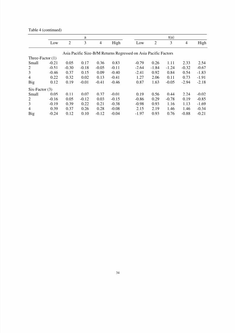
8/3/2019 Size Value and Momentum in International Stock Returns Nov 2010
http://slidepdf.com/reader/full/size-value-and-momentum-in-international-stock-returns-nov-2010 34/38
34
Table 4 (continued)
a t(a)
Low 2 3 4 High Low 2 3 4 High
Asia Pacific Size-B/M Returns Regressed on Asia Pacific Factors
Three-Factor (1)Small -0.21 0.05 0.17 0.36 0.83 -0.79 0.26 1.11 2.33 2.54
2 -0.51 -0.30 -0.18 -0.05 -0.11 -2.64 -1.84 -1.24 -0.32 -0.67
3 -0.46 0.37 0.15 0.09 -0.40 -2.41 0.92 0.84 0.54 -1.83
4 0.22 0.32 0.02 0.13 -0.41 1.27 2.06 0.11 0.73 -1.91
Big 0.12 0.19 -0.01 -0.41 -0.46 0.87 1.63 -0.05 -2.94 -2.18
Six-Factor (3)
Small 0.05 0.11 0.07 0.37 -0.01 0.19 0.56 0.44 2.24 -0.02
2 -0.16 0.05 -0.12 0.03 -0.15 -0.86 0.29 -0.78 0.19 -0.85
3 -0.19 0.39 0.22 0.21 -0.38 -0.98 0.93 1.16 1.13 -1.69
4 0.39 0.37 0.26 0.28 -0.08 2.15 2.19 1.46 1.46 -0.34
Big -0.24 0.12 0.10 -0.12 -0.04 -1.97 0.93 0.76 -0.88 -0.21

8/3/2019 Size Value and Momentum in International Stock Returns Nov 2010
http://slidepdf.com/reader/full/size-value-and-momentum-in-international-stock-returns-nov-2010 35/38
35
Table 5 Summary statistics and intercepts for CAPM, three-factor (1), four-factor (2), and six-factor (3)
regressions to explain monthly excess returns on value-weight market portfolios for North America,
Europe, Japan, and Asia Pacific with global factors, November 1990 to September 2010
The GRS statistic, in Part A, tests whether all intercepts in a set of four regressions are zero; a is the
average intercept; |a| is the average absolute intercept; R2 is the average adjusted R2; and s(a) is the
average standard error of the intercepts. With four portfolios and 239 monthly returns, critical values of the GRS statistic for all four models are: 90%: 1.97; 95%: 2.41; 97.5%: 2.84; and 99%: 3.40. In Part
B, a is the intercept for a region and t(a) is its t-statistic. Part A: Summary statistics
GRS a |a| R2
s(a)
CAPM 2.16 0.07 0.32 0.68 0.20Three-Factor (1) 2.30 0.02 0.30 0.70 0.20
Four-Factor (2) 2.35 0.02 0.30 0.70 0.20
Six-Factor (3) 2.35 -0.06 0.38 0.71 0.21
Part B: Intercepts
a t(a)
NA Europe Japan AP NA Europe Japan AP
CAPM 0.24 0.12 -0.51 0.43 1.98 0.92 -1.76 1.72Three-Factor (1) 0.33 0.02 -0.55 0.30 2.75 0.18 -1.89 1.22
Four-Factor (2) 0.34 0.01 -0.57 0.29 2.83 0.11 -1.91 1.12
Six-Factor (3) 0.32 0.16 -0.89 0.15 2.52 1.19 -2.95 0.57

8/3/2019 Size Value and Momentum in International Stock Returns Nov 2010
http://slidepdf.com/reader/full/size-value-and-momentum-in-international-stock-returns-nov-2010 36/38
36
Table 6 Summary statistics for regressions to explain monthly excess returns on portfolios from sorts on size and momentum, with (5x5) and
without (4x5) microcaps, November 1990 to September 2010
The regressions use the Four-Factor (2) and Six-Factor (3) models with Global and Local Factors to explain the returns on Global, North
American, European, Japanese, and Asian Pacific portfolios formed on size and momentum. The 5x5 results include all five size quintiles, the 4x5
results exclude microcaps. The GRS statistic tests whether all intercepts in a set of 25 or 20 regressions are zero; a is the average intercept; |a| isthe average absolute intercept; R2 is the average adjusted R2; and s(a) is the average standard error of the intercepts. With 25 portfolios and 239
monthly returns, critical values of the GRS statistic for all four models are: 90%: 1.41; 95%: 1.56; 97.5%: 1.69; 99%: 1.86; and 99.9%: 2.26. Global Factors Local Factors
5x5 4x5 5x5 4x5
GRS a |a| R2 s(a) GRS |a| GRS a |a| R2 s(a) GRS |a|
Four-Factor (2)
Global 4.40 0.07 0.14 0.94 0.08 2.56 0.09
NorthAmerica 2.40 0.46 0.46 0.75 0.19 1.22 0.41 2.80 0.12 0.15 0.91 0.11 1.20 0.10
Europe 3.85 0.05 0.21 0.75 0.19 3.04 0.15 3.54 0.07 0.19 0.92 0.10 2.82 0.16
Japan 1.37 -0.56 0.56 0.36 0.38 1.16 0.60 0.82 -0.01 0.10 0.92 0.13 0.68 0.07
AsiaPacific 2.78 0.33 0.43 0.52 0.37 2.33 0.37 3.51 0.27 0.38 0.84 0.21 2.37 0.29
Six-Factor (3)
Global 3.39 0.05 0.14 0.95 0.08 2.33 0.10
NorthAmerica 2.11 0.50 0.50 0.75 0.20 1.32 0.43 2.16 0.13 0.15 0.92 0.11 1.12 0.10
Europe 3.24 0.22 0.24 0.76 0.19 2.54 0.21 2.28 0.06 0.14 0.93 0.10 1.89 0.12
Japan 1.60 -0.98 0.98 0.43 0.38 1.56 1.00 0.83 -0.01 0.09 0.93 0.12 0.79 0.08
AsiaPacific 2.74 0.13 0.35 0.52 0.39 1.99 0.31 2.98 0.29 0.38 0.85 0.21 1.81 0.29

8/3/2019 Size Value and Momentum in International Stock Returns Nov 2010
http://slidepdf.com/reader/full/size-value-and-momentum-in-international-stock-returns-nov-2010 37/38
37
Table 7 Intercepts from four-factor (2), and six-factor (3) regressions to explain monthly excess returns
on portfolios from 5x5 sorts on size and momentum, November 1990 to September 2010
The regressions use the Four-Factor (2) and Six-Factor (3) models with Global and Local Factors to
explain the excess returns on Global, North American, European, Japanese, and Asian Pacific portfolios
formed from independent size and momentum sorts. The table reports intercepts, a, and t-statistics, t(a). a t(a)
Losers 2 3 4 Winners Losers 2 3 4 Winners
Global Size-Momentum Returns Regressed on Global Factors
Four-Factor (2)
Small 0.03 0.22 0.21 0.53 0.80 0.28 1.94 2.63 6.43 6.56
2 -0.01 0.01 -0.08 0.07 0.31 -0.15 0.12 -1.06 1.07 3.98
3 0.10 -0.05 -0.06 -0.16 -0.03 1.15 -0.69 -0.80 -2.03 -0.40
4 0.12 0.01 -0.03 -0.13 0.01 1.17 0.11 -0.37 -1.73 0.12
Big 0.23 0.02 -0.13 -0.07 -0.17 2.38 0.29 -1.74 -1.16 -1.90
Six-Factor (3)
Small 0.22 0.20 0.10 0.38 0.61 2.21 1.72 1.23 4.67 5.25
2 0.19 -0.00 -0.14 -0.02 0.18 3.01 -0.01 -1.84 -0.35 2.78
3 0.22 -0.06 -0.07 -0.23 -0.10 2.61 -0.77 -0.86 -2.83 -1.21
4 0.18 -0.01 -0.07 -0.14 0.02 1.73 -0.10 -0.86 -1.77 0.23
Big 0.08 -0.08 -0.18 -0.03 0.06 0.96 -1.29 -2.41 -0.54 0.88
North American Size-Momentum Returns Regressed on North American Factors
Four-Factor (2)
Small -0.07 0.17 0.37 0.54 0.75 -0.46 1.74 3.88 4.91 4.87
2 -0.05 0.19 0.15 0.03 0.15 -0.44 2.03 1.43 0.26 1.47
3 0.09 0.10 0.08 0.09 0.03 0.65 0.92 0.82 0.81 0.25
4 0.07 0.18 0.13 -0.04 0.05 0.50 1.87 1.26 -0.44 0.40
Big 0.14 0.09 -0.12 -0.03 -0.16 1.16 0.95 -1.19 -0.31 -1.45
Six-Factor (3)
Small 0.16 0.18 0.35 0.45 0.67 1.29 1.84 3.59 3.91 4.30
2 0.14 0.18 0.13 -0.02 0.05 1.53 1.95 1.20 -0.17 0.58
3 0.26 0.13 0.11 0.02 -0.04 2.05 1.19 1.11 0.21 -0.38
4 0.12 0.18 0.19 -0.02 0.12 0.89 1.76 1.83 -0.19 0.94
Big 0.03 -0.02 -0.15 0.02 0.08 0.26 -0.29 -1.47 0.19 0.89

8/3/2019 Size Value and Momentum in International Stock Returns Nov 2010
http://slidepdf.com/reader/full/size-value-and-momentum-in-international-stock-returns-nov-2010 38/38
Table 7 (continued)
a t(a)
Losers 2 3 4 Winners Losers 2 3 4 Winners
European Size-Momentum Returns Regressed on European Factors
Four-Factor (2)Small -0.22 -0.06 -0.10 0.37 0.97 -1.93 -0.63 -0.98 3.98 5.97
2 -0.18 0.09 -0.09 0.10 0.56 -1.92 0.77 -1.05 1.15 4.78
3 0.16 -0.03 0.06 -0.19 0.11 1.45 -0.32 0.60 -2.31 1.03
4 0.22 0.08 0.01 -0.13 0.06 1.58 0.83 0.14 -1.33 0.51Big 0.43 0.09 -0.00 -0.22 -0.30 3.53 0.88 -0.04 -2.57 -2.63
Six-Factor (3)
Small 0.07 0.02 -0.12 0.28 0.52 0.66 0.25 -1.21 2.94 3.57
2 0.06 0.15 -0.10 -0.00 0.19 0.64 1.20 -1.06 -0.05 1.96
3 0.36 0.06 0.09 -0.25 -0.14 3.40 0.66 0.84 -2.85 -1.39
4 0.31 0.12 0.05 -0.11 0.05 2.13 1.26 0.50 -1.06 0.45
Big 0.05 -0.14 -0.03 -0.10 0.07 0.47 -1.35 -0.37 -1.10 0.67
Japanese Size-Momentum Returns Regressed on Japanese Factors
Four-Factor (2)Small 0.31 0.25 0.13 0.18 -0.04 2.10 1.90 1.15 1.44 -0.22
2 0.05 -0.03 -0.02 0.00 -0.01 0.42 -0.32 -0.14 0.01 -0.09
3 -0.00 -0.19 -0.10 -0.02 0.04 -0.03 -1.82 -0.83 -0.13 0.30
4 -0.00 -0.10 -0.12 -0.13 0.04 -0.00 -0.84 -0.99 -1.02 0.30
Big 0.08 -0.15 -0.32 -0.06 0.04 0.50 -1.17 -2.51 -0.57 0.38
Six-Factor (3)
Small 0.26 0.22 0.12 0.19 0.00 2.21 1.84 1.11 1.60 0.03
2 0.02 -0.05 -0.02 0.02 0.03 0.19 -0.56 -0.21 0.17 0.22
3 -0.02 -0.20 -0.10 -0.01 0.06 -0.19 -1.94 -0.84 -0.06 0.45
4 -0.00 -0.10 -0.12 -0.13 0.05 -0.01 -0.84 -0.98 -1.02 0.34Big 0.13 -0.12 -0.32 -0.08 0.01 1.11 -1.05 -2.50 -0.74 0.14
Asian Pacific Size-Momentum Returns Regressed on Asia Pacific Factors
Four-Factor (2)
Small 0.30 0.77 0.77 1.16 0.76 1.69 4.38 4.86 5.55 3.84
2 -0.56 0.18 0.20 0.78 0.15 -3.67 1.08 1.15 2.07 0.813 -0.23 1.02 0.05 0.34 -0.06 -1.27 1.09 0.30 2.08 -0.31
4 -0.15 0.29 0.23 0.23 -0.08 -0.86 1.64 1.44 1.43 -0.41
Big 0.56 0.11 0.17 0.03 -0.31 2.86 0.82 1.10 0.22 -1.76
Six-Factor (3)
Small 0.54 0.80 0.80 1.16 0.55 3.39 4.34 4.84 5.36 2.942 -0.27 0.29 0.30 0.83 -0.10 -1.95 1.69 1.69 2.11 -0.61
3 -0.09 1.17 0.08 0.42 -0.17 -0.47 1.20 0.52 2.44 -1.004 -0.12 0.32 0.30 0.28 -0.17 -0.67 1.77 1.82 1.64 -0.81
Big 0.23 -0.05 0.13 0.26 -0.18 1.35 -0.40 0.80 1.86 -1.01