skew detection correction in scanned document...

Skew Detection & Correction in

Scanned Document Images

Avinash Chandra Kishan

Varun Sharda

Department of Computer Science and Engineering

National Institute of Technology Rourkela

Rourkela-769 008, Orissa, India

Skew Detection & Correction in

Scanned Document Images

Thesis submitted in partial fulfillment

of the requirements for the degree of

Bachelor of Technology

in

Computer Science and Engineering

by

Avinash Chandra Kishan(Roll: 10506001)

Varun Sharda(Roll: 10506055)

Department of Computer Science and Engineering

National Institute of Technology Rourkela

Rourkela-769 008, Orissa, India

May 2009

Department of Computer Science and EngineeringNational Institute of Technology RourkelaRourkela-769 008, Orissa, India.

Certificate

This is to certify that the work in the thesis entitled Skew Detection & Correction In

Scanned Document Images by Avinash Chandra Kishan & Varun Sharda is a record

of an original research work carried out by them under my supervision and guidance

in partial fulfillment of the requirements for the award of the degree of Bachelor of

Technology in Computer Science and Engineering during the session 2005–2009 in the

department of Computer Science and Engineering, National Institute of Technology

Rourkela. Neither this thesis nor any part of it has been submitted for any degree or

academic award elsewhere.

Date: 11 May 2009 Pankaj Kumar SaLecturer

CSE department of NIT Rourkela

Acknowledgment

We would like to gratefully acknowledge the enthusiastic supervision and guidance of

Prof. Pankaj Kumar Sa during this work. His suggestions and constant encourage-

ment proved to be an immense source of motivation.

We are very much indebted to Prof. Banshidhar Majhi, Head-CSE, for alloting us this

project and believing in us. Also for the resources and facilities that were available

to us whenever we needed, that proved to be a vital part of the success of this work.

Our sincere thanks to Prof. S.K. Rath, Prof. S.K. Jena, Prof. B. D. Sahoo, Prof. A.

K. Turuk, Prof. D. P. Mohapatra, Prof. S. Chinara, Prof. P. M. Khilar, Prof. R.

Baliarsingh, and Prof. K. S. Babu for being our knowledge resource. Their help can

never be penned in words.

We would like to thank all our friends , especially Shikhar for helping us. We would

also like to thank all those who have directly or indirectly contributed in the success

of our work.

Last but not the least, NIT Rourkela for providing us such a platform where we

learned a lot and gained so much experience.

Avinash Chandra Kishan

Varun Sharda

Abstract

During document scanning, skew is inevitably introduced into the incoming doc-

ument image. Skew detection is one the first operations to be applied to scanned

documents when converting data to a digital format. Its aim is to align an image be-

fore processing because text segmentation and recognition methods require properly

aligned next lines.

Different algorithms of skew detection are implemented. The first one is Scan line

based skew detection. In this method the image is projected at several angles and

the variance in the number of black pixels per projected scan line is determined. The

angle at which the maximum variance occurs is the angle of skew.

The second one is based on the Hough transform. Hough transform is performed

on the scanned document image and the variance in ρ values is calculated for each

value of θ. The angle that gives the maximum variance is the skew angle.

The third approach is based on the base-point method. Here a concept of base-

point is introduced. After the successive base-points in every text line within a suitable

sub-region were selected as samples for the straight-line fitting. The average of these

baseline directions is computed, which corresponds to the degree of skew of the whole

document image.

All the above mentioned algorithm have been implemented and the results of each

have been compared for accuracy.

Contents

Certificate ii

Acknowledgement iii

Abstract iv

List of Figures vii

List of Tables viii

1 Introduction 1

1.1 Image Processing . . . . . . . . . . . . . . . . . . . . . . . . . . . . . 1

1.2 Document Image Processing . . . . . . . . . . . . . . . . . . . . . . . 3

1.3 Problem Definition . . . . . . . . . . . . . . . . . . . . . . . . . . . . 5

1.4 Motivation . . . . . . . . . . . . . . . . . . . . . . . . . . . . . . . . . 5

1.5 Thesis Organisation . . . . . . . . . . . . . . . . . . . . . . . . . . . . 5

2 Scan Line based Skew Detection 7

2.1 Scan Line . . . . . . . . . . . . . . . . . . . . . . . . . . . . . . . . . 7

2.1.1 Algorithm . . . . . . . . . . . . . . . . . . . . . . . . . . . . . 7

2.2 Time Complexity . . . . . . . . . . . . . . . . . . . . . . . . . . . . . 8

2.3 Hough Transform . . . . . . . . . . . . . . . . . . . . . . . . . . . . . 8

2.3.1 Implementation of Hough Transform . . . . . . . . . . . . . . 14

2.4 Time Complexity . . . . . . . . . . . . . . . . . . . . . . . . . . . . . 15

3 Skew Detection based on Base-Point 20

3.1 Selection of a sub-region and objects . . . . . . . . . . . . . . . . . . 20

3.1.1 Sub-region selection . . . . . . . . . . . . . . . . . . . . . . . . 20

3.1.2 Objects choosing . . . . . . . . . . . . . . . . . . . . . . . . . 21

v

3.2 Base-points clustering . . . . . . . . . . . . . . . . . . . . . . . . . . 22

3.2.1 Definitions . . . . . . . . . . . . . . . . . . . . . . . . . . . . . 22

3.2.2 Base-points clustering . . . . . . . . . . . . . . . . . . . . . . 22

3.3 Time Complexity . . . . . . . . . . . . . . . . . . . . . . . . . . . . . 23

4 Conclusions 28

4.1 Achievements and Limitations of the work . . . . . . . . . . . . . . . 28

4.2 Further Development . . . . . . . . . . . . . . . . . . . . . . . . . . . 29

Bibliography 30

List of Figures

2.1 Deskewed document image of scanned book page with scan line scheme 9

2.2 Deskewed document image of scanned exam paper with scan line scheme 10

2.3 Deskewed document image of scanned telephone directory with scan

line scheme . . . . . . . . . . . . . . . . . . . . . . . . . . . . . . . . 11

2.4 Deskewed images applying the Scan line scheme . . . . . . . . . . . . 12

2.5 Normal Representation of a line . . . . . . . . . . . . . . . . . . . . . 13

2.6 Deskewed document image of scanned book page with the Hough trans-

form scheme . . . . . . . . . . . . . . . . . . . . . . . . . . . . . . . . 16

2.7 Deskewed document image of scanned exam paper with Hough trans-

form scheme . . . . . . . . . . . . . . . . . . . . . . . . . . . . . . . . 17

2.8 Deskewed document image of scanned telephone directory with Hough

transform scheme . . . . . . . . . . . . . . . . . . . . . . . . . . . . . 18

2.9 Deskewed images applying the Hough transform scheme . . . . . . . . 19

3.1 Representation of Bounding-box and Base-point for a scanned character 22

3.2 Deskewed document image of scanned book page with Base-point scheme 24

3.3 Deskewed document image of scanned exam paper with Base-point

scheme . . . . . . . . . . . . . . . . . . . . . . . . . . . . . . . . . . . 25

3.4 Deskewed document image of scanned telephone directory with Base-

point scheme . . . . . . . . . . . . . . . . . . . . . . . . . . . . . . . 26

3.5 Deskewed images applying the Base-point scheme . . . . . . . . . . . 27

vii

List of Tables

2.1 Comparative Results in Skew of different scanned document images as

calculated and original angles (as measured) using Scanline based skew

correction. . . . . . . . . . . . . . . . . . . . . . . . . . . . . . . . . . 8


calculated and original angles (as measured) using Hough Transform

Method. . . . . . . . . . . . . . . . . . . . . . . . . . . . . . . . . . . 15


calculated and original angles (as measured) using Base-Point Method. 23

viii

Chapter 1

Introduction

1.1 Image Processing

The sense of vision has been one of the most vital senses for human survival and

evolution. Humans use the visual system to see or acquire visual information, per-

ceive, i .e. process and understand it and then deduce inferences from the perceived

information. The field of image processing focuses on automating the process of gath-

ering and processing visual information. The process of receiving and analyzing visual

information by digital computer is called digital image processing.

An image may be described as a two-dimensional function I.

I = f(x, y) (1.1)

where x and y are spatial coordinates. Amplitude of f at any pair of coordinates

(x, y) is called intensity I or gray value of the image. When spatial coordinates and

amplitude values are all finite, discrete quantities, the image is called digital image [1].

Digital image processing may be classified into various subbranches based on meth-

ods whose: [1]

• input and output are images and

• inputs may be images where as outputs are attributes extracted from those

images.

Following is the list of different image processing functions based on the above two

classes.

1

1.1 Image Processing

• Image Acquisition

• Image Enhancement

• Image Restoration

• Color Image Processing

• Multi-resolution Processing

• Compression

• Morphological Processing

• Segmentation

• Representation and Description

• Object Recognition

For the first seven functions the inputs and outputs are images where as for the

rest three the outputs are attributes from the input images. With the exception of

image acquisition and display most image processing functions are implemented in

software. Image processing is characterized by specific solutions, hence the technique

that works well in one area can be inadequate in another. The actual solution of a

specific problem still requires a significant research and development [2].

Out of the ten sub-branches of digital image processing, cited above, this thesis

deals with image restoration. In thesis various restoration methodology are used and

various inputs are restored using these methods.

This is chapter is organized as follows. Document Image Processing is discussed

in Section 1.2. The problem definition is described in Section 1.3. Motivation behind

carrying out the work is stated in Section 1.4. Organization of the thesis is outlined

in Section 1.5.

2

1.2 Document Image Processing


Methods for the creation and persistent storage of text have existed since the Mesopot-

amian clay tablets, the Chinese writings on bamboo and silk as well as the Egyptian

writings on papyrus. For search and retrieval, methods for systematic archiving of

complete documents in a library were developed by monks and by the clerks of em-

perors and kings in several cultures. However, the technology of editing an existing

document by local addition and correction of text elements has a much younger his-

tory. Traditional copying and improvement of text was a painstakingly slow process,

sometimes involving many man years for one single document of importance. The

invention of the pencil and eraser in 1858 was one of the signs of things to come.

The advent of the typing machine by Sholes in 1860 allowed for faster copying and

a simultaneous on-the-fly editing of text. The computer, finally, allowed for a very

convenient processing of text in digital form. However, even today, methods for gen-

erating a new document are still more advanced and mature than are the methods

for processing an existing document.

This observation may sound unlikely to the fervent user of a particular common

word-processing system, since creation and correction of documents seems to pose

little problems. However, such a user has forgotten that his or her favorite word-

processor software will only deal with a finite number of digital text formats. The

transformation of the image of an existing paper document - without loss of content

or layout - into a digital format which can be textually processed is mostly difficult

and often impossible. Our user may try to circumvent the problem by using some

available software pack- age for optical-character recognition (OCR). Current OCR

software packages will do a reasonable job in aiding the user to convert the image

into a document format which can be handled by a regular word-processing system,

provided that there are optimal conditions with respect to:

• image quality

• separability of the text from its background image

• presence of standard character-font types

3


• absence of connected-cursive handwritten script and

• simplicity of page layout

Indeed, in those cases where strict constraints on content, character shape and

layout do exist, current methods will even do quite a decent job in faithfully convert-

ing the character images to their corresponding strings of digital character codes in

ASCII or Unicode. Examples of such applications are postal address reading or digit

recognition on bank checks.

On the other hand, if the user wants to digitally process the hand-written diary

of a grandparent or a newspaper snippet from the eighteenth century, the chances of

success are still dim. Librarians and humanities researchers worldwide will still prefer

to manually type ancient texts into their computer while copying from paper rather

than entrusting their material to current text-recognition algorithms. Not only is the

word processing of arbitrary-origin text images a considerable problem. Even if the

goal can be reduced to a mere search and retrieval of relevant text from a large digital

archive of hetero- geneous text images there are many stumbling blocks. Furthermore,

surprisingly, not only the ancient texts are posing problems.

Even the processing of modern, digitally created text in various formats such as

web pages with their mixed encoded and image-based textual content will require

reverse engineering before such a digital document can be loaded into the word pro-

cessor of the recipient.Indeed, classification of text within an image is so difficult that

the presence of human users of a web site is often gauged by presenting them with

a text fragment in a distorted rendering which is easy on the human reading system

but an insurmountable stumbling block for current OCR systems. This weakness of

the artificial reading system thus can be put to good use. The principle is known

as CAPTCHA: Completely Automated Public Turing Tests to Tell Computers and

Humans Apart . During recent years, yet another exciting challenge has become ap-

parent in pattern-recognition research. The reading of text from natural scenes as

recorded by a camera poses many problems, unless we are dealing with a heavily

constrained application such as, e.g., the automatic recognition of letters and dig-

its in snapshots of automobile license plates. Whereas license-plate recognition has

4

1.5 Thesis Organisation

become a mere technical problem, the camera-based reading of text in man-made

environments, e.g., within support systems for blind persons , is only starting to show

preliminary results. [3]

1.3 Problem Definition

Document Image Processing has many different tasks and methods to accomplish

those tasks. During document scanning, skew is inevitably introduced into the in-

coming document image. Skew is any deviation of the image from that of the original

document, which is not parallel to the horizontal or vertical. Skew Correction remains

one of the vital part in Document Processing.

1.4 Motivation

A literature survey of the existing solutions to the problem of skew detection leads to

the following conclusions:

• Solutions that provide accurate skew angles are slow.

• Solutions that reduce the required time result in lesser accuracy in skew angle

determination.

So a trade-off between accuracy and time complexity is the motivation for the

work.


The rest of the thesis is organized as follows:

Chapter 2 proposes two methods of skew detection. One is based on the

scanline method. And the other one based on the Hough transform. This method

outperforms its counterparts in terms of accuracy.

Chapter 3 proposes a method based on the base-point method. But this one

gives more emphasis on the connected component and is more accurate when

the document has clear connected components.

5


Finally Chapter 4 presents the concluding remarks, with scope for further

research work.

6

Chapter 2

Scan Line based Skew Detection

There are various methods to detect skew in an scanned document image. But here

we focus on the methods based on scanline i.e. on the scanline method and on the

Hough transform. Finally the result obtained from our implementation is added.

2.1 Scan Line

This method projects the image at several angles and determines the variation in the

number of black pixels per projected scan line. The angle at which the maximum

variance occurs is the angle of skew. [4]

2.1.1 Algorithm

1. Calculate the coordinates, in the image plane, for each of the parallel scan lines,

that lie at a slope tan(θ) in the image plane.The coordinates are calculated using

the Bresenham’s Line Drawing Algorithm.

2. For each scan line, count the number of non-background pixels that lie on the

line.

3. Calculate the variance v in the number of black pixels that lie on each scan line

for a given angle θ.

4. The angle of skew θ is given by the angle at which the maximum variance vmax

is found.

7

2.3 Hough Transform

Table 2.1: Comparative Results in Skew of different scanned document images ascalculated and original angles (as measured) using Scanline based skew correction.

Angles⇒Calculated Skew (θs) Original Skew (θ)

Scanned Document Images ⇓fig 2.6(a) 3 2

fig 2.6(c) 2 2

fig 3.3(a) −8 −8

fig 3.3(c) 6 6

fig 3.4(a) −7 −7

fig 3.4(c) 15 15

fig 3.5(a) 16 16

fig 3.5(c) −18 −18

The following are the results of the correction figures of the scanned document

images using Scanline based detection : fig. 2.1 , fig. 2.2, fig. 2.3, fig. 2.4

2.2 Time Complexity

Let N be the number of pixels in the scanned document image. Then, the time

complexity is O(N).

2.3 Hough Transform

The Hough transform is an edge linking and boundary detection technique used in

image analysis. The purpose of the technique is to find instances of objects within a

certain class of shapes by a voting procedure. This voting procedure is carried out

in a parameter space, from which object candidates are obtained as local maxima

in a so-called accumulator space that is explicitly constructed by the algorithm for

computing the Hough transform.

Consider a point (xi, yi) in the xy-plane and the general equation of a straight

line in slope-intercept form, yi = axi + b. Infinitely many lines pass through (xi, yi),

but they all satisfy the equation for yi = axi + b for varying values of a and b.

However writing this equation as b = −xia + yi and considering the ab-plane (also

8

2.3 Hough Transform

(a) First scanned image from book (b) Corrected image of (a)

(c) Second scanned image from book (d) Corrected image of (c)

Figure 2.1: Deskewed document image of scanned book page with scan line scheme

9

2.3 Hough Transform

(a) First scanned exam paper image (b) Corrected image of (a)

(c) Second scanned exam paper image (d) Corrected image of (c)

Figure 2.2: Deskewed document image of scanned exam paper with scan line scheme

10

2.3 Hough Transform

(a) First scanned telephone directory image (b) Corrected image of (a)

(c) Second scanned telephone directory image (d) Corrected image of (c)

Figure 2.3: Deskewed document image of scanned telephone directory with scan linescheme

11

2.3 Hough Transform

(a) Third scanned telephone directory image (b) Corrected image of (a)

(c) Fourth Scanned telephone directory image (d) Corrected image of (c)

Figure 2.4: Deskewed images applying the Scan line scheme

12

2.3 Hough Transform

Figure 2.5: Normal Representation of a line

called parameter space) yield the equation of a single line for a fixed pair (xi, yi).

Furthermore, a second point (xj , yj) also has a line in parameter space associated with

it, and unless they are parallel, this line intersects the line associated with (xi, yi) at

some point (a′, b′), where a′ is the slope and b′ the intercept of the line containing

both (xi, yi) and (xj , yj) in the xy-plane. In fact, all the points on this line have lines

in parameter space that intersect at (a′, b′).

In principle, the parameter-space lines corresponding to all points (xk, yk) in the

xy-plane could be plotted, and the principal lines in that plane could be found by

identifying points in parameter space where large numbers of parameter-space inter-

sect. A practical difficulty with this approach, however, is that a (the slope of a line)

approaches infinity as the line approaches the vertical direction. This problem can be

solved by using normal representation of a line:

x cos θ + y sin θ = ρ

Fig. 2.5 represents the geometrical interpretation of the parameters θ and ρ. A

horizontal line has θ = 0°, with ρ being equal to positive x-intercept. Similarly, a

vertical line has θ = 90, with ρ being equal to positive y-intercept or θ = −90, with

ρ being equal to negative y-intercept. Each sinusoidal curve in figure 1.2 represents

the family of lines that pass through a particular point (xk, yk) in the xy-plane. The

intersection point (ρ′, θ′) in fig. 2.5 corresponds to the line that passes through both

(xi, yi) and (xj , yj) in fig. 2.5.

13

2.3 Hough Transform

The computational attractiveness of the Hough Transform arises from subdivid-

ing the ρθ parameter space into so-called accumulator cells where (ρmin, ρmax) and

(θmin, θmax) are the expected ranges of the parameter values: -90°≤ θ ≤ 90°and -D

≤ ρ ≤ D, where D is the maximum distance between opposite corners in an image.

The cell at coordinates (i, j), with accumulator value A(i, j), corresponds to the square

associated with parameter-space coordinates (ρi, θj). Initially, these cells are set to

zero. Then, for every non-background point (xk, yk) in the xy-plane, we let θ equal

each of the allowed subdivision values on the θ axis and solve for the corresponding

ρ using the equation ρ = xkcosθ + yksinθ. The resulting ρ values are then rounded

off to the nearest allowed cell value along ρ axis. If a choice of an angle θq results

in solution ρp, then we let A(p, q) = A(p, q) + 1. The number of subdivisions in the

ρθ-plane determines the accuracy of the collinearity of the points.

The steps for finding skew angle using Hough transform is as follows:

1. For each non-background pixel P (′x′i,′ y′

i).

2. Calculate the corresponding values of ρ, ρj for each −90 <= θi <= 90. The

value of ρ is rounded of to the nearest allowed cell value along ρ axis.

3. Increment the corresponding Hough matrix cell, H(j, i), by one.

The above process results in a Hough matrix, whose each cell, (i, j), gives the

number of points that lie on the line with parameters ρ and θ, (ρi, θj). Each column

of the Hough matrix gives all points that lie on a set of parallel lines, irrespective of

the ρ values. Thus, finding the variance v of the values along each column gives us

the variance in the number of background pixels that lie on a set of parallel scan lines.

Again, the angle of skew is the angle at which this variance is maximum.

2.3.1 Implementation of Hough Transform

An input image is taken and Hough transform was implemented. The value of θ was

incremented across the rows and the value of ρ was incremented across the columns.

The variance was calculated for values in each column i.e. variance in the number of

14

2.4 Time Complexity

Table 2.2: Comparative Results in Skew of different scanned document images ascalculated and original angles (as measured) using Hough Transform Method.


Scanned Document Images ⇓fig 2.6(a) 1 2

fig 2.6(c) 1 2

fig 3.3(a) −8 −8

fig 3.3(c) 6 6

fig 3.4(a) −7 −7

fig 3.4(c) 15 15

fig 3.5(a) 16 16

fig 3.5(c) −18 −18

points between the number of points that lie on a set of parallel lines. The θ that

gave the maximum variance is the skew angle.

The following are the results of the corrected figures of the scanned document

images using hough based detection: fig. 2.7 , fig. 2.8, fig. 2.9

2.4 Time Complexity

Let Nnb be the number of non-background pixels in the scanned document image.

And let Nθ be the number of angles used to calculate the Hough Transform. Then

the time complexity is O(NnbNθ)

15

2.4 Time Complexity

(a) First scanned image from book (b) Resulting image from first scannedimage

(c) Second scanned image from book (d) Resulting image from secondscanned image

Figure 2.6: Deskewed document image of scanned book page with the Hough trans-form scheme

16

2.4 Time Complexity

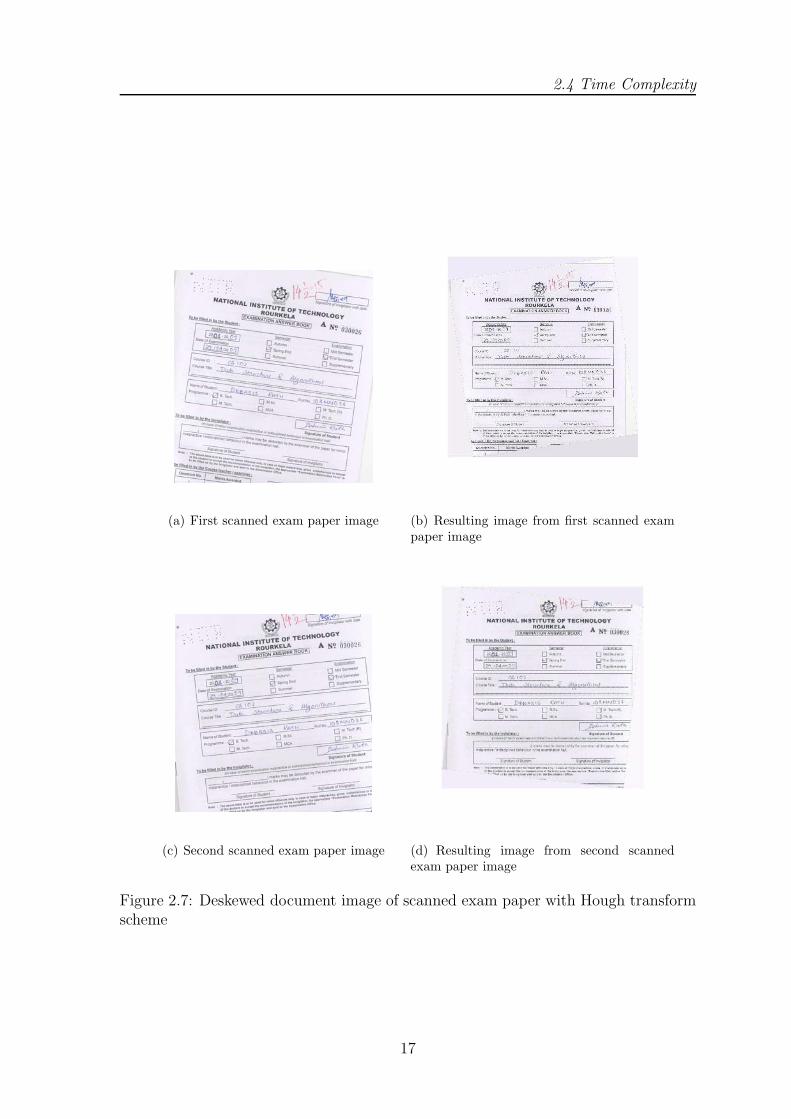
(a) First scanned exam paper image (b) Resulting image from first scanned exampaper image

(c) Second scanned exam paper image (d) Resulting image from second scannedexam paper image

Figure 2.7: Deskewed document image of scanned exam paper with Hough transformscheme

17

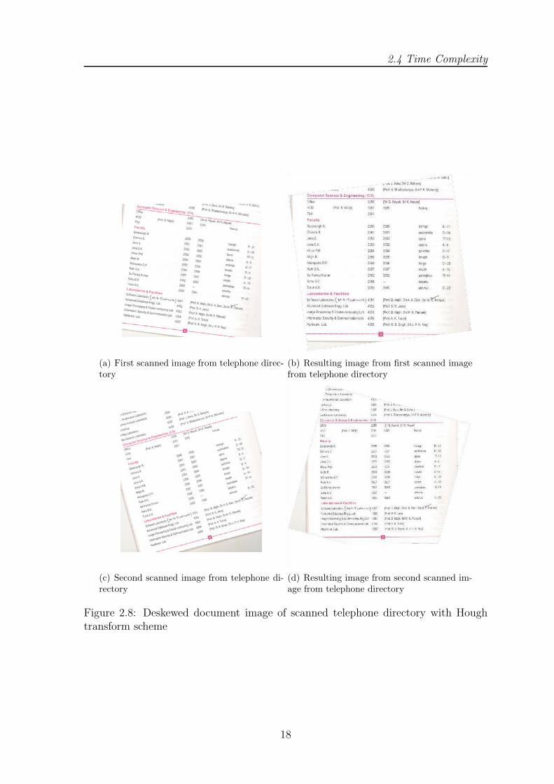
2.4 Time Complexity

(a) First scanned image from telephone direc-tory

(b) Resulting image from first scanned imagefrom telephone directory

(c) Second scanned image from telephone di-rectory

(d) Resulting image from second scanned im-age from telephone directory

Figure 2.8: Deskewed document image of scanned telephone directory with Houghtransform scheme

18

2.4 Time Complexity

(a) Third scanned image from telephone di-rectory

(b) Resulting image from third scanned imagefrom telephone directory

(c) Fourth scanned image from telephone di-rectory

(d) Resulting image from fourth scanned im-age from telephone directory

Figure 2.9: Deskewed images applying the Hough transform scheme

19

Chapter 3

Skew Detection based onBase-Point

In this chapter we are going to discuss the methods of skew detection using a staight

line fitting algorithm. The various steps involved and the additional criteria which

increases the efficiency of these algorithms have been discussed. Finally, the imple-

mentation with suitable examples are given.

3.1 Selection of a sub-region and objects

3.1.1 Sub-region selection

Text lines in a document are generally parallel to one another in the horizontal di-

rection, and the space between two successive text lines is relatively constant. Since

scanning every pixel in the whole document image is time-consuming, it is appropriate

to select a suitable sub-region to calculate the text line direction that corresponds to

the skew angle of the image.

Though pixels in one page image express all kinds of information, it is time-

consuming to analyze all the pixels in the image. Connected component, which is the

aggregation of related pixels, can also express the information in many aspects such

as page layout [5].

In a scanned document image, there might be some black edges that not only

affect the algorithm accuracy but also increase the computing cost. In order to avoid

the possible negative effects of black edges, the edges of a document image should

not be included in the selected sub-region. Furthermore, the size of the sub-region

20

3.1 Selection of a sub-region and objects

should be carefully selected to achieve higher speed and better accuracy. The selected

sub-region R should satisfy the following condition:

R = {(x, y)|w1 ≤ x ≤ w2, h1 ≤ y ≤ h2, (w2 − w1) ≥ Wc, (h2 − h1) ≥ Th} (3.1)

Here Wc is the average width of the alphanumeric characters, and Th is the space

threshold between the successive text lines. Given that the width of a document image

is W and the height is H, the left boundary of the sub-region should be w1 = W/3, the

right boundary w2 = W2/3, the top boundary h1 = H/3 and the bottom boundary

h2 = H2/3. Statistically, the number of connected components in one text line n

should be over 10, and the number of text lines in the subregion k should be more

than 3, which can ensure the precision of this algorithm.

At the same time the relationships between the adjacent connected components are

analyzed with some algorithms such as projection, which can make sure the selected

sub-region contains only one text column.

3.1.2 Objects choosing

The bounding box of every connected component is generated firstly. And a single

character or touched characters contained in the bounding box are regarded as an

object.

Statistically, most of the alphanumeric objects bottoms are on a baseline, such as ′

A′,′ s′,′ x′ , etc. Only a very few alphanumeric objects′ bounding boxes pass through a

baseline, such as ′ p′,′ q′, etc. The sizes of the punctuation mark objects are obviously

smaller than the alphanumeric ones. In order to remove the negative effects of these

punctuation marks, only the objects satisfying the following condition can be selected

as candidates for the skew detection algorithm:

C = {Ci|W (Ci) ≥ Dw ∨ H(Ci) ≥ Dh, 1 ≤ x ≤ k} (3.2)

Here C is the set of candidates for the skew detection algorithm, W (Ci) and H(Ci)

are the width and the height of the bounding box of the object Ci, respectively, Dw

21

3.2 Base-points clustering

Figure 3.1: Representation of Bounding-box and Base-point for a scanned character

is the threshold of the width of the objects′ bounding box, Dh is the threshold of the

height of the objects′ bounding box, and k is the number of candidate objects.

3.2 Base-points clustering

3.2.1 Definitions

Definition 1. Base-point of an object is the center at the bottom within the

bounding box of an object fig. 3.1.

Definition 2. Base-group is a group containing all the base-points in the same

text line.

3.2.2 Base-points clustering

In a pure text sub-region where the text lines are parallel, the base-points in different

text lines can be grouped into different base-groups according to the space threshold

Th. The following is the detailed procedure.

Step 1. Initialize every base-point so that it is not in any base-group, and set

k = 0.

Step 2. In the selected sub-region R, if the lefttop base-point Pi(xi, yi) not in

any basegroup is found, set k + + and put Pi, into a new base-group G(k).

Step 3. Within the rectangle area {(xi, yi − Th/2)}, {(w2, yi + Th/2)}, if the

leftmost base-point Pj(xj , yj) not in any base-group is found, put Pj into G(k)

and set Pi = Pj(i.e.xi = xj , yi = yj). Repeat this step until all the base-points

are in a certain base-group within this rectangle area.

22

3.3 Time Complexity

Table 3.1: Comparative Results in Skew of different scanned document images ascalculated and original angles (as measured) using Base-Point Method.


Scanned Document Images⇓fig 2.6(a) 1 2

fig 2.6(c) 1 2

fig 3.3(a) −4 −8

fig 3.3(c) −2 6

fig 3.4(a) −1 −7

fig 3.4(c) −1 15

fig 3.5(a) −4 16

fig 3.5(c) −3 −18

Step 4. Go to Step 2 until all the base-points in the sub-region R have been put

into different base-groups.

Apply straight line fitting, using least squares method, for each of the cluster ob-

tained at the end of Step 4 to get the slope of the line that is a best fit for each cluster.

Take the average of all slope values obtained in the previous step. This is our skew

angle.

3.3 Time Complexity

Let the number of pixels in the subregion R be NR. Then the base-point algorithm

has a time complexity of O(NR).

23

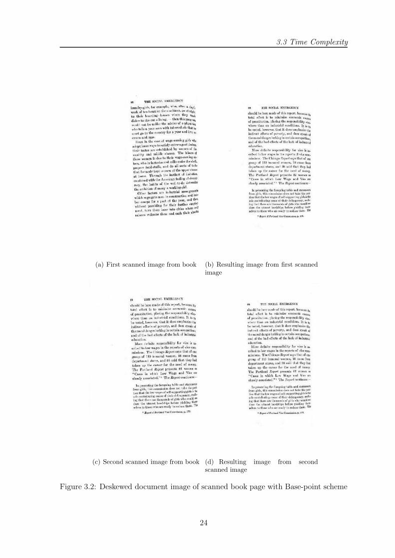
3.3 Time Complexity

(a) First scanned image from book (b) Resulting image from first scannedimage

(c) Second scanned image from book (d) Resulting image from secondscanned image

Figure 3.2: Deskewed document image of scanned book page with Base-point scheme

24

3.3 Time Complexity

(a) First scanned exam paper image (b) Resulting image from first scanned exampaper image

(c) Second scanned exam paper image (d) Resulting image from second scannedexam paper image

Figure 3.3: Deskewed document image of scanned exam paper with Base-point scheme

25

3.3 Time Complexity

(a) First scanned image from telephone direc-tory

(b) Resulting image from first scanned imagefrom telephone directory

(c) Second scanned image from telephone di-rectory

(d) Resulting image from second scanned im-age from telephone directory

Figure 3.4: Deskewed document image of scanned telephone directory with Base-pointscheme

26

3.3 Time Complexity

(a) Third scanned image from telephone di-rectory

(b) Resulting image from third scanned imagefrom telephone directory

(c) Fourth scanned image from telephone di-rectory

(d) Resulting image from fourth scanned im-age from telephone directory

Figure 3.5: Deskewed images applying the Base-point scheme

27

Chapter 4

Conclusions

The work in this thesis, primarily focuses on skew detection in scanned document

images. The work reported in this thesis is summarized in this chapter. Sec. 4.1 lists

the pros and cons of the work. 4.2 provides some scope for further development.

4.1 Achievements and Limitations of the work

The scan line algorithm, based on calculating the coordinates of lines in the image

plane and finding the number of non-background image pixels on a line and then

finding the skew angle on the basis of variance is a successful method, in terms of

skew detection and was found to reliably detect a range of skew angles over a range

of text document images. However, it has a drawback of being painstakingly slow as

compared to the other methods.

The hough transform method was found to be as good as the scan line algorithm

in terms of skew detection and has a much lesser time complexity.

The above two methods were found to provide the correct skew angle even when

the document image consists of many lines that are parallel to the text, since these

lines increase the number of votes because the number of votes along the direction

of these lines is much more as compared to any other direction. These methods are

particularly useful for detecting skews in documents that contain for scripts which

have lines as a major part of the script. For example, many Indian scripts such as

Devanagri, Bangla, Gurmukhi,etc. have lines, called headlines, connecting letters of

a word.

28

4.2 Further Development

The base point method has a much lesser time complexity than the other two,

since it operates on eigen points instead of working on all non-background image

pixels. Since this method relies on connected components to find the eigen points, if

the connected components so found are not distinct characters, the base point method

can result in false results. This was evident in the test images.

4.2 Further Development

The algorithms we have discussed works well with tilted skews and not with shear

skews in scanned document images. We can try to implement and/or modify the

existing algorithm so that it can detect also detect shear skews in scanned document

images.

29

Bibliography

[1] R. C. Gonzalez and R. E. Woods. Digital Image Processing. Addison Wesley, 2nd

edition, 1992.

[2] Anil K. Jain. Fundamentals of Digital Image Processing. Prentice Hall of India,

2008.

[3] Bidyut B. Chaudhuri. Reading Systems: An Introduction to Digital Document

Processing. Springer London, 2007.

[4] Katherine Marsden. Skew detection and correction overview.

http://www.eecs.berkeley.edu/ fateman/kathey/skew.html.

[5] Chandan Singha, Nitin Bhatiab, and Amandeep Kaur. Hough transform based

fast skew detection and accurate skew correction methods. Pattern Recognition,

41:3528 – 3546, 2008.

[6] Yang Cao, Shuhua Wang, and Heng Li. Skew detection and correction in document

images based on straight-line fitting. Pattern Recognition Letters, 24:1871 – 1879,

2003.

[7] Pankaj Kumar Sa. On the Development of Impulsive Noise Removal Schemes.

Master’s thesis, National Institute of Technology Rourkela, 2006.

30

skew detection correction in scanned document...

Documents