sl a - dtic · 2011-05-14 · integration, topology, and geometry in 14 lectures on nielsen fixed...

DTfCSL A LFCI(TR rjJUN I 1993e

C

Inverse Scafferingand Applications

Yt r\ l, - A\

Contemporary Mathematics

Standing orders are accepted for ('oitemporar ' V latt•,natics as well as other bookseries published by the American Mathematical Society. If you are interested in receivingpurchasing information on each new volume in the ContemporarYv Matheumatic's series as itis published, please write or call the American Mathematical Society.

Customer ServicesAmerican Mathematical SocietyPost Office Box 6248Providence, Rhode Island 02940-62481 -800-321 -4AMS (321 -4267) 93....13226

Titles in This Series

Volume

1 Markov random fields and their 13 Algebraists' homage: Papers inapplications, Ross Kindermann and ring theory and related topics,J. Laurie Snell S. A. Amitsur, D. J. Saltman, and

2 Proceedings of the conference on G. B. Seligman, Editors

integration, topology, and geometry in 14 Lectures on Nielsen fixed point theory,linear spaces, William H. Graves, Editor Boju Jiang

3 The closed graph and P-closed 15 Advanced analytic number theory.graph properties in general topology, Part 1: Ramification theoretic methods,T. R. Hamlett and L. L. Herrington Carlos J. Moreno

4 Problems of elastic stability and 16 Complex representations of GL(2, K) forvibrations, Vadim Komkov. Editor finite fields K, Ilya Piatetski-Shapiro

5 Rational constructions of modules 17 Nonlinear partial differential equations.for simple Lie algebras, George B. Joel A. Smoller, EditorSeligman 18 Fixed points and nonexpansive

6 Umbral calculus and Hopf algebras, mappings, Robert C. Sine, EditorRobert Morris, Editor 19 Proceedings of the Northwestern

7 Complex contour integral homotopy theory conference, Haynesrepresentation of cardinal spline R. Miller and Stewart B. Priddy, Editorsfunctions, Walter Schempp 20 Low dimensional topology, Samuel J.

8 Ordered fields and real algebraic Lomonaco, Jr., Editorgeometry, D. W. Dubois and T. Recio, 21 Topological methods in nonlinearEditors functional analysis, S. P. Singh,

9 Papers in algebra, analysis and S_ Thomeier, and B. Watson. Editorsstatistics, R. LidI, Editor 22 Factorizations of bn ± 1, b = 2,

10 Operator algebras and K-theory, 3, 5,6,7,10,11,12 up to highRonald G. Douglas and Claude powers, John Brillhart, D. H. Lehmer,Schochet, Editors J. L. Selfridge, Bryant Tuckerman, and

11 Plane ellipticity and related problems, S. S. Wagstaff, Jr.Robert P. Gilbert, Editor 23 Chapter 9 of Ramanujan's second

12 Symposium on algebraic topology in notebook-Infinite series identities,honor of Jose Adem, Samuel Gitler, transformations, and evaluations,Editor Bruce C. Berndt and Padmini T. Joshi

93


Volume24 Central extensions, Galois groups, and 43 Group actions on rings, Susan

ideal class groups of number fields, Montgomery, EditorA. Frohlich 44 Combinatorial methods in topology and

25 Value distribution theory and its algebraic geometry, John R. Harperapplications, Chung-Chun Yang, Editor and Richard Mandelbaum, Editors

26 Conference in modern analysis 45 Finite groups-coming of age, Johnand probability, Richard Beals, McKay, EditorAnatole Beck, Alexandra Bellow, and Mctay, EditorArshag Hajian, Editors 46 Structure of the standard modu(esfor the affine Lie algebra (•1),

27 Microlocal analysis, M. Salah Baouendi, James L 1epo ie algebra A.

Richrd Bals andLina PrissJames Lepowsky and Mirko PrimcRichard Beaals, and Linda Preiss

Rothschild, Editors 47 Linear algebra and its role in28 Fluids and plasmas: geometry and systems theory, Richard A. Brualdi.

28yFluids, and rold psMarsdety aditr David H. Carlson, Biswa Nath Datta,dynamics, Jerrold E. Marsden, EditorChreR.JnsadRortJCharles R. Johnson, and Robert J.

29 Automated theorem proving, W. W. Plemmons, EditorsBledsoe and Donald Loveland, Editors 48 Analytic functions of one complex

30 Mathematical applications of category variable, Chung-chun Yang andtheory, J. W. Gray, Editor Chi-tai Chuang, Editors

31 Axiomatic set theory, James E.Baumgartner, Donald A. Martin, and no Cnmplex differential geometry andSaharon Shelah. Editors nonlinear differential equations,

Yum-Tong Siu. Editor32 Proceedings of tho conference on

Banach algebras arid several complex 50 Random matrices and theirvariables, F. Greeneaf and D. Gulick, applications, Joel E. Cohen,Editors Harry Kesten, and Charles M. Newman.Edditors

33 Contributions to group theory, Editors

Kenneth I. Appel. John G. Ratcliffe, and 51 Nonlinear problems in gzometry,Paul E. Schupp. r*'rr Dennis M. DeTurck, Editor

34 Combinatorics and algebra, Curtis 52 Geometry of normed linear spaces,Greene, Editor R. G. Bartle, N. T. Peck. A. L. Peressini,

35 Four-manifold theory, Cameron Gordon and J. J. Uhl, Editors

and Robion Kirby, Editors 53 The Selberg trace formula and related

36 Group actions on manifolds, Reinhard topics, Dennis A. Hejhal, Peter Sarnak.Schultz, Editor and Audrey Anne Terras, Editors

37 Conference on algebraic topology in 54 Differential analysis and infinitehonor of Peter Hilton, Renzo Piccinini dimensional spaces, Kondaguntaand Denis Sjerve, Editors Sundaresan and Srinivasa Swaminathan,

38 Topics in complex analysis, Dorothy EditorsBrowne Shaffer, Editor 55 Applications of algebraic K-theory to

39 Errett Bishop: Reflections on him and algebraic geometry and number theory,his research, Murray Rosenblatt, Editor Spencer J. Bloch, R. Keith Dennis, Eric

40 Integial bases for affine Lie algebras M. Friedlander, and Michael R. Stein.

and their universal enveloping algebras, Editors

David Mitzman 56 Multiparameter bifurcation theory,

41 Particle systems, random media and Martin Golubitsky andlarge deviations, Richard Durrett, Editor John Guckenheimer, Editors

42 Classical real analysis, Daniel 57 Combinatorics and ordered sets,Waterman, Editor Ivan Rival, Editor


Volume

58.1 The Lefschetz centennial conference. 74 Geometry of group representations,Proceedings on algebraic geometry, William M. Goldman and Andy R. Magid,D. Sundararaman, Editor Editors

58.11 The Lefschetz centennial conference. 75 The finite calculus associated withProceedings on algebraic topology, Bessel functions, Frank M. CholewinskiS. Gitler. Editor 76 The structure of finite algebras,

58.111 The Lefschetz centennial conference. David C. Hobby and Ralph Mckenzie

Proceedings on differential equations, 77 Number theory and its applications inA. Verjovsky, Editor China, Wang Yuan, Yang Chung-chun,

59 Function estimates, J. S. Marron, Editor and Pan Chengbiao, Editors

78 Braids, Joan S. Birman and Anatoly60 Nonstrictly hyperbolic conservationLigerEdtr

laws, Barbara Lee Keyfitz and

Herbert C. Kranzer, Editors 79 Regular differential forms, Ernst Kunzand Rolf Waldi

61 Residues and traces of differential 90 Statistical inference 1rom stochasti-forms via Hochschild homology, processes, N. U. Prabhu, EditorJoseph Lipman 81 Hamiltonian dynamical systems,

62 Operator algebras and mathematical Kenneth R. Meyer and Donald G. Saari,physics, Palle E. T. Jorgensen and EditorsPaul S. Muhly, Editors 82 Classical groups and related topics,

63 Integral geometry, Robert L. Bryant, Alexander J. Hahn, Donald G. James,Victor Guillemin, Sigurdur Helgason, and and Zhe-xian Wan, EditorsR. 0. Wells, Jr., Editors 83 Algebraic K-theory and algebraic

64 The legacy of Sonya Kovalevskaya, number theory, Michael R. Stein andLinda Keen, Editor R. Keith Dennis, Editors

65 Logic and combinatorics, Stephen G. 84 Partition problems in topology,Simpson, Editor Stevo Todorcevic

66 Free group rings, Narian Gupta 85 Banach space theory, Bor-Luh Lin,

67 Current trends in arithmetical algebraic Editor

geometry, Kenneth A. Ribet, Editor 86 Representation theory and numbertheory in connection with the local

68 Differential geometry: The interface Langlands connecture, J. Rither, Editor

between pure and applied mathematics, 8 Abelan goupethe , L z Fuche ,

Mladen Luksic, Clyde Martin, and 87 Abelian group theory, Laszlo Fuchs,

William Shadwick, Editors REdiger Gsbel, and Phillip Schultz,Editors

69 Methods and applications of 88 Invariant theory, R. Fossum,mathematical logic, Walter A. Carnielli W. Haboush, M. Hochster, andand Luiz Paulo de Alcantara, Editors V. Lakshmibai, Editors

70 Index theory of elliptic operators, 89 Graphs and algorithms, R. Brucefoliations, and operator algebras, Richter, EditorJerome Kaminker, Kenneth C. Millett, 90 Singularities, Richard Randell, Editorand Claude Schochet, Editors90SnuaiisRcarRndlEto91 Commutative harmonic analysis,

71 Mathematics and general relativity, David Colella, EditorJames A. Isenberg, Editor 92 Categories in computer science and

72 Fixed point theory and its applications, logic, John W. Gray and Andre Scedrov,R. F. Brown, Editor Editors

73 Geometry of random motion, Rick 93 Representation theory, group rings, andDurrett and Mark A. Pinsky, Editors coding theory, M. Isaacs. A. Lichtman,


VolumeD. Passman, S, Sehgal, N. J. A. Sloane, 111 Finite geometries and combinatorialand H. Zassenhaus, Editors designs, Earl S. Kramer and Spyros S.

94 Measure and measurable dynamics, Magliveras, EditorsR. Daniel Mauldin, R. M. Shortt, and 112 Statistical analysis of measurementCesar E. Silva, Editors error models and applications,

95 Infinite algebraic extensions of finite Philip J Brown and Wayne A. Fuller,fields, Joel V. Brawley and George E. EditorsSchnibben 113 Integral geometry and tomography,

96 Algebraic topology, Mark Mahowald Eric Grinberg and Eric Todd Quinto,

and Stewart Priddy, Editors Editors97 Dynamics and control of multibody 114 Mathematical developments arising

systems, J. E. Marsden, P.S. from linear programming, Jeffrey C.

Krishnaprasad, and J. C. Simo, Editors Lagarias and Michael J. Todd. Editors98 Every planar map is four colorable, 115 Statistical multiple integration,

Kenneth Appel and Wolfgang Haken Nancy Flournoy and Robert K.

99 The connection between infinite Tsutakawa, Editors

dimensional and finite dimensional 116 Algebraic geometry: Sundance 1988,icolaenko, Brian Harbourne and Robert Speiser,dynamical systems, Basil Editorsko

Ciprian Foias, and Roger Temam, Editors

Editors 117 Continuum theory and dynamical

100 Current progress in hyperbolic systems: systems. Morton Brown, Editor

Riemann problems and computations, 118 Probability theory and its applications inW. Brent Lindquist, Editor China, Yan Shi-Jian, Wang Jiagang, and

101 Recent developments in geometry, Yang Chwtg-chun, Editors

S.-Y. Cheng, H. Choi, and Robert E. 119 Vision geometry, Robert A. Melter,Greene, Editors Azriel Rosenfeld, and Prabir

102 Primes associated to an ideal, Bhattacharya, Editors

Stephen McAdam 120 Selfadjoint and nonselfadjoint operatoralgebras and operator theory,

103 Coloring theories, Steve Fisk Robert S. Doran, Editor104 Accessible categories: The foundations 121 Spinor construction of vertex operator

of categorical model theory, Michael algebras, triality, and E Alex J.Makkai and Robert Part) 8lers raiy n () lxJFeingold, Igor B. Frenkel, and John F. X.

105 Geometric and topological invariants Riesof elliptic operators, Jerome Kaminker, 122 Invese scattering and applications,Editor 0. H. Sattinger, C. A. Tracy, and S.

106 Logic and computation, Wilfried Sieg, Venakides, EditorsEditor

107 Harmonic analysis and partialdifferential equations, Mario Milmanand Tomas Schonbek, Editors

108 Mathematics of nonlinear science,Melvyn S. Berger, Editor

109 Combinatorial group theory, BenjaminFine, Anthony Gaglione, and FrancisC. Y. Tang, Editors

110 Lie algebras and related topics,Georgia Benkart and J. Marshall Osborn,Editors

Inverse Scatteringand Applications

' """ A & I/,. ' TA&

NDisri

Di t A vl/ O-d O

7 M.

CONTEMPORARYMATHEMATICS

122

Inverse Scatteringand Applications

Proceedings of a Conferenceon Inverse Scattering on the Line

held June 7-13, 1990at the University of Massachusetts, Amherst

with support from the National Science Foundation,the National Security Agency,

and the Office of Naval Research

D. H. SattingerC. A. Tracy

S. VenakidesEditors

American Mathematical SocietyProvidence, Rhode Island

EDITORIAL BOARD

Richard W. Beals, managing editorSylvain E. Cappell Linda Preiss RothschildCraig Huneke Michael E. Taylor

The AMS-IMS-SIAM Joint Summer Research Conference in the MathematicalSciences on Inverse Scattering on the Line was held at the University of Mas-sachusetts, Amherst, Massachusetts, on June 7-June 13, 1990 with support fromthe National Science Foundation, Grant DMS-8918200, National Security AgencyMDA904-90-H-402. This work relates to Department of Navy Grant N00014-90-J-1157 issued by the Office of Naval Research. The United States Government hasa royalty-free license throughout the world in all copyrightable material containedherein.

1991 Mathematic,, Subject Classification. Primary 34825. 35P25, 35R30.

Library of Congress Cataloging-in-Publication Data

AMS-IMS-SIAM Joint Summer Research Conference in the Mathematical Sciences on InverseScatttering on the line (1990: University of Massachusetts, Amherst)

Inverse scattering and applications/[edited by] David Sattinger, Craig Tracy, StephanosVenakides.

p. cm.-(Contemporary mathematics)"Proceedings of AMS-IMS-SIAM Joint Summer Research Conference in the

Mathematical Sciences on Inverse Scattering on the Line, held June 7-13, 1990 at theUniversity of Massachusetts, Amherst, Massachusetts.

ISBN 0-8218-5129-2 (alk, paper)1. Inverse problems (Differential equations) -Congresses. 2. Scattering

(Mathematics) -Congresses. I. Sattinger, David H. II. American Mathematical Society.tli. Institute of Polathematical Statistics. IV. Society for Industrial and Applied Mathematics.V. Title. VI. Series.QA370.A57 1990 91-26094515'.353-dc2O CiP

Copying and reprinting. Individual readers of this publication, and nonprofit librariesacting for them, are permitted to make fair use of the material, such as to copy an article foruse in teaching or research. Permission is granted to quote brief passages from this publicationin reviews, provided the customary acknowledgment of the source is given.

Republication, systematic copying, or multiple reproduction of any material in this pub-lication (including abstracts) is permitted only under license from the American MathematicalSociety. Requests for such permission should be addressed to the Manager of Editorial Ser-vices, American Mathematical Society, P.O. Box 6248, Providence, Rhode Island 02940-6248.

The appearance of the code on the first page of an article in this book indicates thecopyright owner's consent for copying beyond that permitted by Sections 107 or 108 of theU.S. Copyright Law, provided that the fee of $1.00 plus $.25 per page for each copy be paiddirectly to the Copyright Clearance Center, Inc., 27 Congress Street, Salem, Massachusetts01970. This consent does not extend to other kinds of copying, such as copying for generaldistribution, for advertising or promotional purposes, for creating new collective works, or forresale.

Copyright (1991 by the American Mathematical Society. All rights reserved.The American Mathematical Society retains all rights except those granted

to the United States Government.Printed in the United States of America.

The paper used in this book is acid-free and falls within the guidelinesestablished to ensure permanence and durability. G

This volume was prepared using AVIS-TEX,the American Mathematical Society's TEX macro system.

Some of the articles were prepared by the authors.

10987654321 969594939291

Contents

Preface xi

Wiener-Hopf Factorization in Multidimensional Inverse SchrodingerScattering

TUNCAY AKTOSUN AND CORNELIS VAN DER MEE 1

Complete Integrability of "Completely Integrable" SystemsRICHARD BEALS AND DAVID SATTINGER 13

On the Determinant Theme for Tau Functions, Grassmannians, andInverse Scattering

ROBERT CARROLL 23

An Overview of Inversion Algorithms for Impedance ImagingMARGARET CHENEY AND DAVID ISAACSON 29

On the Construction of Integrable XXZ Heisenberg Models With

Arbitrary SpinHOLGER FRAHM 41

A Geometric Construction of Solutions of Matrix Hierarchies

G. F. HELMINCK 47

Lax Pairs, Recursion Operators, and the Perturbation of NonlinearEvolution Equations

RUSSELL HERMAN 53

Time and Temperature Dependent Correlation Function of Impen-etrable Bose Gas Field Correlator in the Impenetrable Bose Gas

A. R. ITS, A. G. IZERGIN, AND V. E. KOREPIN 61

Breathers and the sine-Gordon EquatiorSATYANAD KICHENASSAMY 73

Localized Solitons for the Ishimori EquationB. G. KONOPELCHENKO AND V. G. DuBROVSKY 77

ix

(CONTENTS

Tau FunctionsJOHN PALMER 91

Inverse Problems in Anisotropic MediaJOHN SYLVESTER AND GUNTHER UHLMANN 105

The Toda Shock ProblemSTEPHANOS VENAKIDES 119

Preface

This conference covered a variety of topics in inverse problems: inverse scatteringproblems on the line; inverse problems in higher dimensions: inverse conductivityproblems: and numerical methods. In addition, problems from statistical physicswere covered, including monodromy problems, quantum inverse scattering, and theBethe ansatz. One of the aims of the conference was to bring together researchers ina variety of areas of inverse problems. All of these areas have seen intensive activityin recent years.

Inverse conductivity problems

This class of problems was discussed by David Isaacson and Margaret Cheney ofRenssalaer Polytechnic Institute and by Gunther Uhlmann of the University of Wash-ington. Uhlmann discussed his work with John Sylvester on the problem of determin-ing anisotropic conductivities in a region from measurements made on the boundary.These measurements may include the Dirichlet-Neumann map or knowledge of thegeodesics. Margaret Cheney discussed various algorithms for reconstructing the con-ductivities from the data: these included iterative methods, and Calderon's methods.David Isaacson discussed experimental work being carried oat at Renssalaer Poly-technic Institute and ended his talk with an intriguing videotape of actual inverseimaging experiments on a human subject (himself).

Adrian Nachman, of the University of Rochester, gave an overview of inversescattering and conductivity problems. Joyce McLaughlin, of Renssalaer Polytech-nic Institute, presented recent results on inverse spectral problems for second orderdifferential operators.

Numerical methods

Vladimir Rokhlin of Yale University described a numerical algorithm for inversescattering based on a Riccati equation for the impedence function combined with cer-tain trace formulae for the unknown functions. Numerical experiments performed inonc dimension have shown themselves to be stable, rigorous, and extremely efficient.He hopes to be able to extend the methods to two and three dimensional problems.

Soliton problems

One dimensional inverse scattering methods are a fundamental tool in the theoryof completely integrable systems. Percy Deift of the Courant Institute opened the

'I

xii PREFACE

conference with a beautiful summary of the theory of inverse scattering for nth orderordinary differential operators. Thanks to recent work by Xin Zhou and Deift, thistheory is now complete. Thomas Kappeler of Brown University discussed actionangle variables for the periodic KdV equetion. Richard Beals of Yale Universityspoke on his recent work with D. Sattinger on action angle variables for integrablesystems based on first order n x n isospectral operators. The construction of actionangle variables for these infinite dimensional completely integrable systems is ,asedon the scattering transform.

Scattering theory was also used by Bjorn Birnir of University of California. SantaBarbara and S. Kichenessamy of the Courant Institute in their (independent) workshowing that only the Sine-Gordon equation can support breather solutions.

M. Wickerhauser of the University of Georgia reported on joint work with R. Coif-man of Yale University on some of the special problems of the scattering transformfor the Benjamin-Ono equation. Their work gives estimates for some previouslyformal work associated with the Benjamin-Ono hierarchy.

S. Venakides of Duke University reported on joint work with P. Delft of theCourant Institute and R. Oba of Tulane University on the Toda Shock problem.Long time asymptotic analysis of the explicit solution is carried out by the inversescattering method. Residual oscillations are derived and analyzed when the initialvelocity exceeds a critical value. The results are in agreement with earlier numericalexperiments by Straub and Holian, znd Flaschka and McLaughlin.

David McLaughlin of Princeton University discussed chaos and heteroclinic orbitsof perturbed integrable systems.

Three dimensional problems

A. Ramm of Kansas State University and T. Aktosun of the University of Texas atDallas presented their work on three dimensional problems. Ramm talKed about theC Property and Aktosun talked on the Wiener-Hopf factorization of the scatteringoperatoi in three dimensions, based on ideas of R. Newton.

Statistical physics

A number of problems in statistical physics lead to problems involving inversemonodromy or inverse scattering, and several of the talks addressed these areas.V. Korepin, of the University of New York at Stonybrook, discussed correlationfunctions for the quantized version of the nonlinear Schrodinger equation. In manycases, the correlation functions satisfy nonlinear differential equations of Painlevetype. The Pinlevý equations, in turn, are associated in a direct way with certainmonodromy problems; in fact, the monodromy problems play a role analogous tothe isospectral operators in the theory of completely integrable systems. Inversemonodromy problems thus play an important role. John Palmer of the Universityof Arizona talked about the Cauchy Riemann operators associated with such inversemonodromy problems and their infinite dimensional determinants as tau functions

PREFACE xiii

for the problem. The tau functions are in fact the partition function of statisticalmechanics. Hank Thacker of the University of Virginia talked about related topicsincluding spin chains and vertex models. Craig Tracy spoke on monodromy problemsin higher dimensions, specifically some isomonodromy problems for the Laplacianon the Poincare disk. The two point correlation function can be expressed in termsof Painleve VI.

During the course of the conference, Persi Diaconis, who was attending the otherconference at Amherst. overheard mention of the "Bethe ansatz" during an informaldiscussion at coffee break. It developed that there was a connection between the or-der/disorder transitions in "card shuffling" problems that Diaconis has been workingon, and the Bethe ansatz method used in connection with the statistical problemsbeing discussed by Korepin and Thacker. Diaconis agreed to give a special lecture.at 8:30 a.m. Sunday morning, on his work on order/disorder transitions. Severaldiscussions resulted, and a round table session took place on Monday evening tounderstand the relationships.

D. 14. Sattinger

Contemporary MathematicsVOlume 122, 1991

WIENER-HOPF FACTORIZATION

IN MULTIDIMENSIONAL INVERSE SCHR6DINGER SCATTERING'

Tuncay Aktosun2 and Cornelis van der Mee 3

ABSTRACT. We consider a Riemann-Hilbert problem arising in the study of the in-

verse scattering for the multidimensional Schr6dinger equation with a potential having

no spherical symmetry. It is shown that under certain conditions on the potential, the

corresponding scattering operator admits a Wiener-Hopf factorization. The solution of

the Riemann-Hilbert problem can be obtained using a similar factorization for the unitar-

ily dilated scattering operator. We also study the connection between the Wiener-Hopf

factorization and the Newton-Marchenko integral operator.

1. RIEMANN-HILBERT PROBLEM IN QUANTUM SCATTERING. Consider the

n-dimensional Schrbdinger equation (n > 2)

(1.1)AV + k2 V(X)

where x E R'. A is the Laplacian. k2 is energy. and V(x) is the potential. In nonrelativistic

quaritum mechanics the behavior of a particle in the force field of V(x) is governed by (1.1).

Mathematics Subject Classification (1991). 35Q 15. 81U05, 35R30. 47A40.'This );Pper is in final form and no version of it will be submitted for publication

elsewhere. . 1, authors are indebted to Roger Newton for his help.2The author is supported by the National Science Foundation under grant DMS

9001903.3The author is supported by the National Science Foundation under grant DMS

8823102.0 1991 Anwrican Mathematical Sovity

0271-4132/91 SO()O + $21) per page

"2 TUNCAY AKTOSUN AND CORNELIS VAN DER MEE

We assunme that V (x) - 0 as jai -' -x in some sense which will be Itiade precise il the

next paragraph, but we do not assume any spherical symmetry for V(x). As Ix! - x, the

wavefunction ii behaves as

r',(k,.x.) = e'9-" + if., I Ikx xYA(k, •-. 9) + o(. J

where O E S-'7 - is a unit vector in R7' arid A(k.O9O') is the scarttring anplir de. The

scattering operator S(k) is defined as

kS(k.O.G') = 6(0 - 0') + i( •-) (k. , W'.

2~r

where 6 is the Dirac delta distribution. In operator notation the above equation bec(omes

k t-IS(k) = I + A(k).

All our results presented in this paper hold for real and locally square-integrable

potentials V(x) E L' (R') belonging to the class Bc, with 0 < o < 2. Here B,. Qk E [0.2).3 t lr:)I{ )i o n e

denotes the class of potentials such that for some s > - ; (I + IT)AV(X) is a bounded

linear operator from H0 (R'n) into L2(R'), where H'(Rf) denotes the Sobolev space

of order (-. For the reader whose interest is restricted to the case it = 3. the following

conditions on the potential will be sufficient:

1. There exist positive constants a and b such that for all y E R3 we have

J dxIV(x)I (xkI+j.y+ a2 < b.

2. There exist constants c > 0 and s > 1/2 such that IV(x)I !__ (11 + jxj 2 )-" for allE 3,

.3. There exist constants -. > 0 and 3 E (0. 1] such that , dx JxI3 ]VJ(x)l < "•.

4. k = 0 is not an exceptional point. This condition is satisfied if there are neither bound

states nor half-bound states at zero energy.

The inverse quantum scattering problem consists of recovering the potential 1*(.) for

all x when S(k) is known for all k. Information about molecular, atomic. and sutbatomic

particles is usually obtained from scattering experiments. An important problem in physics

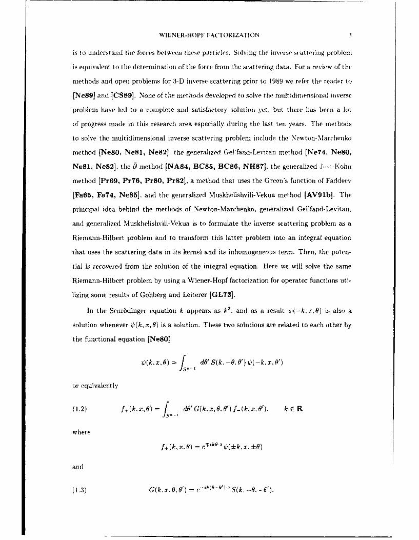
WIENER-HOPF FAC7"ORIZATION 3

is to understand tihe forces between these parficles. Solving the inverse scattering problem

is equivalent to the determination of the force from the scattering data. For a review of the

methods and open problems for 3-D inverse scattering prior to 1989 we refer the reader to

[Ne89] and [CS89]. None of the methods developed to solve the multidimensional inverse

problem have led to a complete and satisfactory solution yet. but there has been a lot

of progress made in this research area especially during the last ten years. The methods

to solve the multidimensional inverse scattering problem include the Newton- Marchenko

method (Ne8O, Ne8l, NeS2]. the generalized Gel'fand-Levitan method [Ne74, Ne8O,

Ne81, Ne82j. the j method [NA84, BC85, BC86, NH871, the generalized J,, Kohn

method [Pr69, Pr76, Pr8O, Pr82], a method that uses the Green's function of Faddeev

[Fa65, Fa74, Ne85], and the generalized Muskhelishvili-Vekua method [AV91b]. The

principal idea behind the methods of Newton-Marchenko. generalized Geffand-Levitan.

anrd generalized Muskhelishvili-Vekua is to formulate the inverse scattering problem as a

Riemann-Hilbert problem and to transform this latter problem into an integral equation

that uses the scattering data in its kernel and its inhomogeneous term. Then, the poten-

tial is recovered from the solution of the integral equation. Here we will solve the same

Riemann-Hilbert problem by using a Wiener-Hopf factorization for operator functions uti-

lizing some results of Gohberg and Leiterer [GL731.

In the Sclir6dinger equation k appears as k2. and as a result V,(-k,x.0) is also a

solution whenever i(k, x, 0) is a solution. These two solutions are related to each other by

the functional equation [Ne8OI

4(k.x.0) = - dO' S(k. -0.0') ý,(-kx,O')

or equivalently

(1.2) f+(k,x,0) f dO'G(k,x,0. 0')f-(k,x,0'), k ER

where

f±(k,x. 0) = eTtkOexmV(±k, x. ±0)

and

(1.3) G(k, T. O. 0') = e-k(°-G') `S(k, -0 -6').

4 TUNCAY AKTOSUN AND CORNELIS VAN DER MEF

For potentials specified in the beginning of this section, in the absen(re of boiund ut ate,.-

f± has an analytic extension in k E C±. If there are bound states, these c'an be renioved

by the reduction technique [Ne89] before the analysis is carried out. Let us supprss thie

x-dependence and write (1.2) in vector form as

f,(k) = G(k)f_(k). k E R,

or equivalently as

(1.4) X+(k) = G(k) X_(k) + [0(k) - 111, k E R.

where

X±(k) = f± (k) - 1.

For potentials considered in this paper X± C L 2 (Sn-1), the Hilbert space of square in-

tegrable functions on S". and the strong limit of f± is i as k - x in C±. Note that

in our notation I denotes the identity operator on L 2 (S- 1 ) and 1 denotes the vector in

L 2(S,-l) such that i{() -1 for 0 E Se-l. Hence. (1.4) constitutes a Riemann-Hilbert

problem: Given G(k). determine X±(k). Note also that from (1.3) it is seen that G(k) is

the unitarily dilated scattering operator.

2. SOLUTION OF THE RIEMANN-HILBERT PROBLEM. We have the following

result concerning the Wiener-Hopf factorization of the operator G(k) that appears in the

Riexnann- Hilbert problem (1.4). In order to keep the discussion short, we assumne that

there are no bound states. If there are bound states. these can be removed by a reduction

technique [Ne8O, Ne89] before the factorization is accomplished, For details we refer the

reader to [AV90].

THEOREM I. For potentials as specified in Section 1. G(k) defincd in (13) has a (left)

Wiener-Hopf factorization: i.e.. there exist operators G+(k) G.. (k). and D(k) such that

G(k) = G,(k) D(k) G_(kj where

1. G. (k) i.s continuous in C- in the operator norm of £(L2(S"-')) and is houndcdly

invertible there. Here C(L 2 (S - I)) denotes the Banach ipace of linear operators acting on

WIENER-H()PF FA(CTORIZATION

L2(q"-l). Similarly, G (k) is contiuous en C In tihe optrator norm of CLW'( " `) i) aned

is boundedly ti'ertible there.

2. G.(k) is analytic in C' and G,_(k) Is analytic in C-

3. (;(±x):=(G_(+x) =I.

4. D(k) - fl + =l - P u hre ... P are rn utually disjoint, rank-oru pro-

jections, and PI = I - EZ..• P'. Thc (left) partial indi'cs Pi p... p,,, are' nlozelo entgcres.

InI custe there arc no partial indic's: ;i... when D(k) = I. the resulting Wgtener-1fopf fac-

toirizatiiO bc•omecs cano cwd.l

Note that. as seen from (1.3). G(k) is a unitary transform of the scattering operator

S(k). In particular, when x = 0. G(k) reduces to S(k). The proof of Theorem I uses sonie

results of Gohberg and Leiterer regarding factorization of operator functions on cont ours in

the complex plane [GL73]. When S(k) is boundedly invertible, is a compact pert urbation

of the identity, ani Sd(•) = S(iL - ) is uniforily H6Mder continuous on the unit circle T

in the complex plane. its unitary transform G(k) also satisfies these three conditions and

admnits a Wieuer-Hopf factorization. The Hhlder-continuity of S(ý) and G(() = G(i )

can he established using either an additive representation of the scattering amplitude or a

multiplicative representation. We refer the reader to [AV90] for the proof that uses an ad-

ditive representation of the scattering amplitude and to [AV91a] for the proof that uses a

multiplicative representation of the scattering amplitude. The conditions on the potential

in 3-I) specified iin Section 1 were used in the additive representation, and the conditions

specified in that section in n-D were used in the multiplicative representation. We also

refer the reader to [Ne90 for various results related to the Wiener-Hopf factorization of

the scattering operator: in this reference Professor Newton introdtuced a related factor-

ization called the Jost finction factorization and studied the relationship between these

two factorizations: in this reference Theorem 5.1 gives a characterization of the scattering

operator for the existence of a potential.

Tlee solution of the Riemann-Hilbert problem (1.4) is obtained in terms of the Wiener-

liopf factors of G(k) [AV9o] and is given a;s

(2.1) X+(k) = [G+(k) - Ii + G+(k) Z ) (kW +i),1) >

A )

6 TUNCAY AKTOSUN AND CORNELIS VAN DER MEL

(2.2) X(k) = [G(k)_' - Ii + G(k) 1 z Oj(k)7r + [(k + )"'- (k - i)'j1P)i>0 (k - i)Pj

provided Pj i = 0 whenever pj < 0. Here 7rT is a fixed nonzero vector in the range of Pf.

and 0,(k) is all arbitrary polynomial of degree less than pj associated with each p, > 0.

We can state our result as follows.

THEOREM 2. For potentials as specified in Section 1. the Riemann-Hilbert problem (1.4)

has a solution if and only if P, 1i = 0 it whenever pj < 0. When this happens. the solution

is given by (2.1) and (2.2). The solution, if it exists, is unique when the operator G(k) has

no positive partial indices.

A simple condition that assures the unique solvability of tile Riemann-Hilbert prob-

lem (1.4) is given by SUPkER JUS(k) - IIl < 1, where the norm is the operator norm in

£(L2(Sn-1)). If this holds, neither the scattering operator S(k) nor its unitary transform

G(k) has any partial indices. As a result, in this case, (1.4) is uniquely solvable.

3. PARTIAL INDICES. In this section we relate the partial indices of the unitar-

ily dilated scattering operator given in (1.3) to the Newton-Marchenko integral operator

[Ne89]. We also discuss the relationship between solutions of the Rieniann-Hilbert prob-

lern and the Newton-Marchenko integral equation. The proofs of the results stated in this

section will be published elsewhere.

We let Q be the operator on L2(Sn-') such that (Qf)(O) = f(-O). As in [Ne89] we

define

(3.1) G(a) f ol e dk-ik- [G(k) - I]O

and we also define the operators g, g. and H" on L2(R+)

(3.2) (GO)(a) - / d/3G(a + /3)71(13), ,i > 0

(33•) (fr,)(a) J d/•G(-a - /3) r'(/3), a > 0

(1 1)('H ) = dil G(-( + /3) ir(fl), a > 0.

WIENER-HOPF FAtTORIZATION 7

The Fourier transform maps L2(R-) onto the Hardy space of analytic operator fute-

tions X+(k) on C+ such that

sup dk IIX+(k + i ()IIL,(S-1) < +*-.

We will denote this Hardy space by H+.

Defining

Sdke-ikaX+(k)27r jIC

f (a) =dk e-zck[G(k) - I]i.

from (1.4) we obtain

(3.4) q(C) = dO G(a + 0) 7(f0) + Q77(-a) + f(a), a E R.

Since X+ E H•. we have 71(a) = 0 for a < 0. Hence. we see that (3.4) is equivalent to

( 1(a) = f d/3 G(a + 3) il(/3) + f•(a). a > 0(3.5)

0=1 d3G(-a+MT)i(3)+Q'q(a)+f(-a), a> 0.

We can write (3.5) in the form

(3.6) { (Q+•'0= -fp

where f*(a) = f(-a). Since (1.4) and (3.6) are equivalent, it follows that every solution

X+ E Ht of the Riemann-Hilbert problem (1.4) leads to a solution q E L2(R÷) of (3.6).

and conversely. The first equation in (3.6) is the Newton-Marchenko integral equation and

G is the Newton-Marchenko integral operator.

Since d(ý) is Hh1der continuous on T. G(ý) - I is a compact operator, and G(ý) is

boundedly invertible for all ý E T, it follows that G(k) has a (left.) Wiener-Hopf factor-

ization [GL73, AV90, AV91a]. In that case., we can solve the Riemann-Hilbert problem

(1.4) in terms of the Wiener-Hopf factors of G(k) and obtain the following [AV90, AV91aI.

PROPOSITION 3. There are finitely many, namely E,, >0 pj, linearly independent solu-

tons of the homogeneous problem (1.4) where F(k) = 0. The inhomoqeneous terms F(k)

8 TUNCAY AKTOSUN AND CORNELIS VAN DER MEE

for which at least one solution of the Riemann-Hilbert problem (1.4) exzsts. form a closed

subspace of L2 (R) of co-dimension equal to - Ep) <0 P.'

Due to the fact that (1.4) and (3.6) are equivalent problems. the above results imply

that for all f,f* E L2 (R+), we have the following.

COROLLARY 4. There are EP, >0 Pj linearly independent solutions 7' of the homogeneous

problem (Q + -)y = 0. The right-hand sides -f* for which at least one solution rq of the

equation (Q +i*)77 = -f* exists, form a closed subspace of L2(R') of finite co-dimension

equal to - EP3 <0 P,"

The partial indices of the operator G(k) given in (1.3) is related to the Newton-

Marchenko operator G as in the following theorem. Note that g and G* are defined in

(3.2) and (3.3).

THEOREM 5. The partial indices of G(k) satisfy

Z Pi = dim Ker (I - 9) + dim Ker (I + 9).p" >0

- Z pj =dim Ker (I- g*) + dim Ker (I+ ).p, <0

Hence, G(k) has a canonical factorization if and only if 1 and-I are not eigenvalues of!P

andS*.

Combining the result of Theorem 5 given above and the results in Lemma 4.3 and

Theorem 4.7 in [Ne90]. we have the following result. In the absence of bound states. for

potentials whose scattering operators belong to the admissible class defined in [Ne90].

there are no partial indices. Also using Theorem 5 above and Corollary 4.5 in [Ne9O], we

see that not only the sum index of G(k) is independent of x (AV90, AV91a], but also the

sum of the negative partial indices of G(k) is independent of x and the sum of the positive

partial indices of G(k) is independent of x. Since supkER JIG(k) -Ill = SuPkER IIS(k) - I11.

noting that G(k) = S(k) for x = 0. it also follows that ! and 9* do not have eigenvalues

1 if suPkER iIS(k) - Ill < 1. Thus. the Newton-Marchenko integral equation is uniquely

solvable if SuPkER fIS(k) - Ill < 1. Here the norm)s are the operator norm on L2(S,-I),

4. CONCLUSION. If the potential in (1.1) causes bound states. the analysis given

in Sections 1, 2. and 3 remains valid. provided we replace G(k) by the reduced operator

WIENER-HOPF FACTORIZATION 9

G"et(k) obtained after removing the bound states by the redtuction technique of Newton

[Ne89, AV90]. Theorem 5 given in Section 3 remains valid for G(k) even in the presence

of bound stvttes.

Combining the result of Theorem 5 given above and the result in Lemma 4.3 in [Ne90],

we have the following result. When there are bound states, for potentials whose scattering

operators belong to the admissible class defined in [Ne90], the number of bound states K

for the Schr6dinger equation (1.1) is related to the sum of the negative partial indices of

G(k) as

AK= - p.Pj <0

For the same class of potentials, there are still no positive partial indices of G(k).

Using Theorem 5 above and Corollary 4.5 in [Ne90], it follows, even if there are

bound states, that both the sum of the negative partial indices of G(k) and that of the

positive partial indices of G(k) are independent of x.

BIBLIOGRAPHY

[AV90] T. Aktosun and C. van der Mee, Inverse Scattering Problem for the 3-D Schri6dinger

Equation and Wiener-Hopf Factorization of the Scattering Operator, J. Math. Phys.

31, 2172-2180 (1990).

[AV91a] T. Aktosun and C. van der Mee, Wiener-Hopf Factorization in the Inverse Scattering

Theory for the n-D Schrddinger Equation, Operator Theory: Advances and Applica-

tions 50, 1 -21 (1991).

[AV91b] T. Aktosun and C. van der Mee, Solution of the Inverse Scattering Problem for the

3-D Schridinger Equation Using a Fredhoim Integral Equation, SIAM J. Math. Anal.

22. 717 731 (1991).

[BC85] R. Beals and R. R. Coifman. Multidimensional Inverse Scattering and Nonlinear

P.D.E. 's, Proc. Symp. Pure Math. 43, 45- 70 (1985).

[BC86] R. B1als and R. R. Coifman, The D-bar Approach to Inverse Scattering and Nonlinear

Evolutions, Physica D 18, 242 249 (1986).

10 TUNCAY AKTOSUN AND CORNELIS VAN DER MEE

[CS89] K. Chadan and P. C. Sabatier, Inverse Problems in Quantum Scattering Theory. 2nd

ed., Springer, New York, 1989.

[Fa65] L. D. Faddeev, Increasing Solutions of the Schrddinger Equation. Soy. Phys. Dokl.

10, 1033-1035 (1965) tDokl. Akad. Nauk SSSR 165, 514--517 (1965) (Russian)].

[Fa74] L. D. Faddeev, Three-dimensional Inverse Problem in the Quantum Theory of Scat-

tering. J. Soy. Math. 5, 334-396 (1976) [Itogi Nauki i Tekhniki 3. 93- 180 (1974)

(Russian)].

[GL73] I. C. Gohberg and J. Leiterer, Factorization of Operator Functions with Respect to a

Contour. I11. Factorization in Algebras, Math. Nachrichten 55, 33-61 (1973) (Rus-

sian).

[NA84] A. I. Nachman and M. J. Ablowitz, A Multidimensional Inverse Scattering Method,

Studies in Appl. Math. 71, 243-250 (1984).

[Ne74] R. G. Newton, The Gel'fand-Levitan Method in the Inverse Scattering Problem in

Quantum Mechanics. In: J.A. Lavita and J.-P. Marchand (Eds.), Scattering Theory

in Mathematical Physics, Reidel, Dordrecht, 1974, pp. 193-225.

[Ne80] R. G. Newton, Inverse Scattering. II. Three Dimensions, J. Math. Phys. 21, 1698-

1715 (1980); 22, 631 (1981): 23, 693 (1982).

[Ne81] R. G. Newton, Inverse Scattering. III. Three Dimensions, Continued, J. Math. Phys.

22, 2191-2200 (1981); 23, 693 (1982).

[Ne82] R. G. Newton, Inverse Scattering. IV. Three Dimensions: Generalized Marchenko

Construction with Bound States, J. Math. Phys. 23, 2257--2265 (1982).

[Ne85] R. G. Newton, A Faddeev-Marchenko Method for Inverse Scattering in Three Dimen-

sions, Inverse Problems 1, 371-380 (1985).

[Ne89] R. G. Newton, Inverse Schrndinger Scattering in Three Dimensions, Springer, New

York, 1990.

[Ne90] R. G. Newton, Factorizations of the S Matrix, T. Math. Phys. 31, 2414--2424 (1990).

WIENER-HOPF FACTOR IZATION I1

[NH87] R. G. Novikov and G. M. Henkin. Solution of a AMultidimensional Inerse Scattering

Problem on the Basis of Generalized Dispersion Relations. Soy. Math. DokA. 35,

153 157 (1987) [Dokl. Akad. Nauk SSSR 292. 814 818 (1987) (Russian)].

[Pr69] R. T. Prosser, Flrmal Solution of Inverse Scattering Problems, J. Math. Phys. 10.

1819- 1822 (1969).

[Pr76] R. T. Prosser, Formal Solution of Inverse Scattering Problems. II, J. Math. Phys.

17, 1775--1779 (1976).

[Pr80] R. T. Prosser, Formal Solution of Inverse Scattering Problems. III, J. Math. Phys.

21, 2648--2653 (1980).

[Pr82] R. T. Prosser, Formal Solution of Inverse Scattering Problems. IV, J. Math. Phys.

23, 2127-2130 (1982).

Tuncay Aktosun Cornelis van der Mee

Department of Mathematics Department of Physics and Astronomy

Southern Methodist University Free University

Dallas. TX 75275 Amsterdam, The Netherlands

Contemporary MathemnaticsVolume 122, 1991

Complete integrability of "Completely Integrable" systems

Richard BealsDavid Sattinger

There is a well-known hierarchy of commuting flows associated with an n x n spectralproblem in one variable. These flows are Hamiltonian with respect to natural symplecticand Poisson structures on the manifold of potentials. It is common to speak of completeintegrability. in analogy with classical mechanics, although in the infinite dimensionalcase there is no question of the number of independent commuting flows being half thenumber of degrees of freedom.

The scattering transform linearizes these flows and decouples the spectral modes.but for n > e it does not trivially decouple the symplectic and Poisson structures.We find action-angle variables which do decouple these structures and thus show thatthe system on the scattering side is a direct integral of finite dimensional completelyintegrable systems. for general n.

An important tool is the analysis of a natural 2-form and symplectic foliation ofSL(n). Reductions of the system require further analysis. e.g. in SU(n). As an appli-cation we obtain the complete integrability of the three wave interaction equation andnote that even on the scattering side one must adjoin a nonlinear flow at each mode inorder to have a complete system of commuting Hamiltonian flows.

The detailed version of this paper will be published elsewhere.

This is an expository account of results concerning the classical complete inte-grability of nonlinear evolution equations which are solvable by the inverse scatteringor inverse spectral method. The method allows the question of complete integra-bility to be posed and (sometimes) answered in a finite-dimensional setting. In theprocess one encounters an interesting 2-form and symplectic foliation on classicalLie groups.

Section 1 gives the classical background and a discussion of the KdV equation.The n x n spectral problem and the associated Hamiltonian flows are described insection 2 and the main theorems are stated. The proofs depend on an analysis ofa 2-form and symplectic foliation on the groups SL(n) and SU(n). described insection 3. Details will appear in [BS1].

f1. Complete integrability in dimensions 2N. 2, and x.Classically a Hamiltonian flow with N degrees of freedom is described in suitable

*Research supported by NSF Grants DMS-8916968 and 8901607S9' % .1fiatheiwjari Sutiect (cau.vofwattion. 35Q55. 38F07.

This paper is in final form and no version of it will he submitted for publication elsewhere,

Q 1991 Amnqrica Matlheatical Sojiety(1271-4132/91 $1. 00 + $.25 per pag'

13

14 RICHARD BEALS AND DAVID SATTINGER

coordinates (x _ .. r. ..Y1. YN) by Hamilton's equations

OH OH(!.) JJ oyj ' = 3

The structure of these equations is linked to the geometry of the symplectic form

Q = E dxj A dy,

and the dual Poisson bracket for functions

= (Of D9 Of Og

Dxj Oyj DY, Xj

In fact, an arbitrary function changes along the trajectories (1.1) according to itsPoisson bracket with the Hamiltonian function H:

f={fH}.

The flow (1.1) is said to be completely integrable if there are N independent integralsof the motion which are in involution, i.e. functions I, .... , I, such that

(1,2) {Ij, H } = O = {I, Ik }, dlI A ... A dIN $ O.

It was shown by Liouville that (1.2) is equivalent to the existence of action-anglevariables for (1.1): coordinate functions P,.... PN, qI ..... qN such that

{pj, H} = O. Q = E dpj A dqj.

The last condition can be written in terms of the Poisson bracket as

(1.3) {pj.qk} = bjk: {PJ.Pk} = {qj,qk} = 0.

In fact. one may take pj = Ij,. and Liouville's method finds the qj by quadratures[WI.

Any Hamiltonian flow with 1 degree of freedom is completely integrable: takeI, = H (if dH : 0). An example is the mathematical pendulum

(1.4) ý = -- sin x, c = constant.

with y = i and H(x. y) = ½y 2 - c cos x. Action-angle variables for (1.4) are Jacobielliptic functions. Equation (1.4) appears in a natural but surprising way for thescattering data for the 3-wave interaction equation: see end of §2.

Sormewhat more generally. a system of k commuting flows with HamiltoniansHI..... Hk in involution is completely integrable if there are N independent func-tions I which are invariant under each flow and in involution with each other.

The question of complete integrability in a nontrivial nonlinear infinite-dimensionalcontext first. arose in c(onnection with the KdV equation

(1.5) ut - 6uu, + u, = 0.

"COMPLETELY INTEGRABLE- SYSTEMS 15

Kruskal and co-workers discovered that (1.5) has a countable family of polynomialconservation laws

au a.i = 0 I = ek(u, TX ..... )k1,)d.

It was shown hv Gardner [Ga] that (1.5) is a Hamiltonian flow with respect to thePoisson bracket(1.7) {F.G} = f ±(T d x:

I T,I TdX 6u d

moreover the constants of motion 1k in (1.6) are in involution. Of course one canno longer simply count degrees of freedom to see whether there are enough Ik's forcomplete integrability. However. Gardner. Greene. Kruskal, and Miura [GGKMihad shown that (1.5) can be integrated exactly by using the scattering theory ofthe linear spectral problem

(1.8) , t(X. t, 4) + (ý2 - tl(X. t)]N(X. t. 4) = 0.

In fact. ignore the t-dependence for a moment and suppose u vanishes at x- inx. Then for real 4. (1.8) has solutions C,± - exp(±ix4) as x - ±x. and thesesolutions are related by

(1.9) .(.4) = a(4)v,(x. -4) + b(j)_(x.4). 1a2 - b= 1.

In the absence of -'int spectrum, the potential u can be recovered from tihe reflectioncoefficient b/a IF). i. the potential u(.. t) evolves according to (1.6). then a. b evolveaccording to(1.10) a(ý.t) = 0. b(ý.t) = 8i43 b(4.t).

at 5

This suggests that the modulus and argument of b might serve as action-anglevariables. Indeed the complete integrability of KdV was established by Zakharovand Faddeev [ZF] by showing that the functions

(1.11) p(4) = log Ia(4)12 = " log[1 + jb(4)121, q(4) = arg b(4)

it 7r

satisfv the continuous version of (1.3):

(1.12) {p(4).q(71)} = 6(4 - q), {p(4).p(71)} = {q(4).q(TI)} = 0.

The equations (1.10) show that the scattering data a. b not only linearize the KdVflow, but also decouple the modes ý. Similarly (1.12) shows that the scatteringdata decouple the Hamiltonian structure (1.7) as a direct integral of 2-dimensionalstructures. Combining the two. one has decomposed KdV as a direct integral of

Hamiltonian flows with I degree of freedom.


There are now a large number of physically interesting nonlinear evolutionequations which are known to be similar to KdV in the following ways (see. e.g.[BuC]. [NMPZ]):

(a) they are Hamiltonian with respect to a Poisson structure similar to(1.7):

(b) there is a countable family of conserved quantities like (1.6) which arein involution:

(c) there is an associated linear spectral problem whose scattering theory (ifknown) gives a procedure for solving the nonlinear initial value problemexactly.

Such equations and systems are commonly called -integrable" or. because of(a), (b), "completely integrable". It is (c), however, which allows one to pose thequestion of complete integrability in a very precise sense: does the scattering dataprovide action-angle variables? This is essentially a finite-dimensional question, atleast after the fact, because for each appropriate value of the spectral parameter ý.the scattering data lives in a finite-dimensional space. In most of the cases where theanswer was known, the dimension of this space is two. so in some sense the problemis reduced to the trivial case of classical complete integrability. Examples are KdV,the cubic nonlinear Schrodinger equation [ZM21. the sine-Gordon equation [FT1].or any equation whose spectral problem is a 2 x 2 system of AKNS-ZS type: see[FT2]. The complete integrability of the 3-wave interaction equation, linked to a3 x 3 system, was investigated by Manakov [M].

In the remainder of this paper, we discuss n x n systems and the associatedflows. Proofs will appear elsewhere [BS1]. In a separate paper [BS2] we provecomplete integrability of the Gelfand-Dikii flows [GD]. These flows are associatedto eigenvalue problems for higher order ordinary differential operators and includethe Boussinesq equation. In this paper. as in the discussion of the KdV flow above,we consider only the case of purely continuous spectral data. Discrete data poses a

different type of question, which is studied in [BK].§2. The n x n spectral problem; flows; scattering dataThe isospectral problem is

(2.1) vQ(x, z) = zJo(x, z) + q(x)O(x, z). z E C. V)(x, z) E GL(n. C).

The potential q is off-diagonal with Schwartz-class entries and J is diagonal withdistinct eigenvalues. General references are [BY], [BC1], [BC21, [C]. [Ge]. [Ne].[Sal, [Sh].

The question of complete integrability can be reduced to the case J + J* = 0.which we now assume. We also reorder rows and columns so that

J = diag(iAi,-.. ,iA). A1 > A2 > . > A,.

"-COMPLETELY INTEGRABLE- SYSTEMS 17

There is a Haamiltonian structure on the manifold of potentials q given by thesymplectic form and Poisson bracket

(2.2) Q = tr{ bq(x) A [adJ] 1 6q(x)Idx,

(2.3) {F,G} = tr [J. 6F, dx.

bqbq

For each traceless constant diagonal matrix p there is a hierarchy of flows

(2.4) 4 = [J, Fk+1,,]

where the Fk,, are polynomials in q and its derivatives [Sal which are definedrecursively by

Fo.I ; [J, Fk+l,•,] = dFk- + [q, Fk•,], lim Fk+±,1t(x) = 0.

The flows (2.4) are Hamiltonian and in involution.For real ý there are normalized solutions V)±(x, ý) of (2.1) linked by the scatter-

ing matrix s(ý) E sl(n, C):

(2.5) lim P±+(x, ) exp[-xýJ] = 1, ¢_(x,V) = + )(8 E R.

Iff flq(x)[ldx < 1 then the scattering map q - s is injective. Under the flow (2.4),the scattering matrix evolves linearly:

(2.6) i(ý, t) = t)].

A complication is that s is subject to nonlocal constraints: the upper (resp. lower)principal minors of s are boundary values of functions which are holomorphic in thelower (resp. upper) half plane. This reflects the fact that the potential q maps theline to a space of dimension n2 - n. while the scattering matrix s maps to a spaceof dimension n2 - 1. Minimal scattering data can be obtained from s by factoring

(2.7) s± = sv+, s+ and v- are upper triangular,

sq and v+ are lower triangular, (v±)j, = 1.

The scattering data (v+, v- ) is a map to a space of dimension n2 - n. The scatteringmatrix s can be reconstructed from (v+, v-) by a process which includes solvingn - 1 scalar Riemann-Hilbert factorization problems.

18 RICHARD BEALS AND DAVI) SATTINGER

In terms of scattering data, the symplectic form and Poisson bracket are

(2.8) Q JR tr[v+i'(bv) A 9+' bs+ - v-1 (bv_) A s- _ bs]

(2.9){Sjk(0), S1m(7l)} =7r iSjm(0js8k(z)[sgn(f- j) - sgn(rn - k)]b(ý - r/)

1+ Sjk()Sfm(T[hft - 6kn] P.V. 1 -

where sgn(O) = 0 and p.v. denotes the principal value, [BC2], [BSI]. See [M] forthe Poisson bracket in the case n = 3 and [Sk], [KDI for R-matrix formulations.

THEOREM A. There are functions a ,, b,, I < v < (n12 - n) defined on a dense

open subset of SL(n, C) such that the composed functions p, = a1, o s. q, = b, o sare action-angle variables for the flows (2.4): the Hamiltonian for (2.4) is a linearcombination of the functionals f ýIp•,(ý)dý and

(2.10) = : Jd p, A dq1,

(2.11) {p(,() r)} = ( 6q) 6,(, - i); {p,()p.,((j)} = {q),q1 ,(vl)} 0.

In the case n = 2, there are just two functions which can be taken to be

(2.12) p(0) = log[s1(0)s22(W)], q(ý) = i 1og[s12 (0)/s2 1(0)]:

in the general case the pu, and iq , can be taken to be logarithms of products andratios of suitable minors of s.

This gives complete integrability of (2.4) in the complex sense. The most im-portant examples for (2.4) involve reduction. i.e. restriction to a submanifold ofthe manifold of potentials q, for which the form is real. An important case is thereduction

(2.13) q(x) + q(x)* = 0

which leads to real f2 and to s(ý) E SU(n). In this case. one would like real action-angle variables. The functions given above for n = 2 are real on SU(2). but ingeneral. real action-angle variables necessarily involve more complicated functionsof the matrix entries.

"COMPLETELY IN FEGRABLE- SYSTEMS 19

THEOREM B. With n = 3, the functions a•, and b, in Theorem A can be chosenso as to be real on SU(n).

This proves complete integrability for the 3-wave interaction. A different ap-proach. using nonlocal functions of s(•), was taken by Manakov [M].

One should note the following: the flows (2.4) do not constitute a full set ofcommuting Hamiltonian flows in any sense. when n > 3. The minimal scatteringdata has pointwise dimension I(n 2 -_1). while the space of flows (2.6) has pointwisedimension n- 1 (complex dimensions in the general case, real dimensions in thecase of the reduction (2.13)). The flows associated to the additional constants ofthe motion are not linear in the scattering data (as elements of the linear spaceMi(C)). Thus for n > 3 the existence of the infinite family of commuting flows(3.4) is not in itself very convincing evidence of complete integrability.

A final remark: under the natural third flow occuring in Theorem B to sup-plement the two linear flows (2.6) at a given point ý, the modulus IS22(0)1 is fixed,while arg s22(0) obeys the pendulum equation (1.4)!

§3. A 2-form and symplectic foliation on SL(n) and SU(n).Given s in SL(n) = SL(n. C), or SL(n, R). denote the upper and lower princi-

pal minors by

(3.1) d+(s) = det(sjk)j.k<c; d-((s) = det(sik)j,k>-.

If no d:y(s) vanishes, s has two unique factorizations (2.7). In terms of these fac-torizations. we may define a 2-form on (a dense open subset of) SL(n) by adapting(2.8):

(3.2) Q, = tr[v+1 (dv+) A s+lds+ - vZ-'(dv_) A s-'dsj1.

As a form on SL(n). it is not obvious that On is closed; it is certainly not symplectic,since the rank in a neighborhood of the identity is n2 - n.

THEOREM C. There are functions pL, qi,, 1 < v < 1.(n 2 - n), such that

(3.3) Q, = E dp,, A dqz,.

In particular. fl,1 is closed.

Although the proof of this theorem is purely algebraic, it is motivated by ob-servations from scattering theory. First, the result is not difficult when n = 2: p,and q, can be chosen as in (2.12). Second, the general result should follow fromthe result for n = 2. because the matrix J of section 2 can be taken as a limitof -generic" complex J for which the scattering data are 2 x 2 matrices living on

(7n2 - n) lines in the complex plane [BC1). These ideas lead to a multiplicativedecomposition of v = v11-v+ and a corresponding additihe decomposition of Q,


The functions (3.1) lead to a natural foliation of SL(n) by the functions

(3.3) pj(s) = d+(s)/d-+l(s), 1 < j < n.

PROPOSITION. The foliation of SL(n) by the functions (3.3) is sympL.,ctic for 9in.i.e. the pullback of Q,, to each leaf is a symplectic form on the leaf.

The symplectic foliation gives a (degenerate) Poisson structure ( , ) onSL(n): on each leaf L the symplectic structure determines a bracket ( )L andthe global bracket ( ) is characterized by

(fg)4L - (f=L,glL)"

It follows from (3.2) that

(3.4) (Pqqv) = 61Av, (pt,,P,,p) = (q,,,q,,) = 0.

As one might begin to expect. the functions denoted p,,, q•, here are the functionsdenoted a,, b, in Theorem A. This is further confirmed by the fact that the Poissonbracket ( . ) is the local part of the Poisson bracket as computed in (2.9):

THEOREM D. The Poisson bracket of matrix elements is given by

(3.5) (s3A = 1 S [sgn(i - j) - sgn(m - k)]? sgn(0) = 0.

The formula (3.5) was first calculated for n = 2 and n = 3 by Lu [L]. whoconjectured the general formula and pointed out its relation to the classical limit ofa quantum group structure defined in [D]. The proof in the general case proceedsthrough a reduction to the cases n < 4.

To complete the proof of Theorem A, one needs to show that the possiblenonlocal terms in (2.11) vanish.

The 2-form fn makes sense as a complex 2-form on SU(n), but it can be shownthat

(3.6) iil,7 is a real 2-form on SU(n).

Moreover, the foliation functions (3.3) have modulus 1 on SU(n). so the foliationis determined by their arguments and thus the Poisson bracket -i(fg) is real onSU(n) when the functions f and g are real.

THEOREM E. For SU(3) the functions p•, and q, in Theorem C can be chosen sothat p, and iq, are real.

In fact one can choose pj = loglsjjI and the qj may be found by Liouville'smethod: they are elliptic functions of the matrix entries; see [BS1].

"COMPLETELY INTEGRABLE" SYSTEMS 21

REFERENCES

[BY] D. Bar Yaacov, Analytic properties of scattering and inverse scatteringfor first order systems. Dissertation, Yale 1985.

[BC1] R. Beals and R.R. Coifman. Scattering and inverse scattering for firstorder systems. Comm. Pure Appl. Math. 37 (1984), 39-90.

[BC2] R. Beals and R.R. Coifrnan. Scattering and inverse scattering for firstorder systems. II. Inverse Problems 3 (1987), 577-593.

[BK] R. Beals and B.G. Konopelchenko, On nontrivial interactions and com-plete integrability for soliton equations, preprint.

[BS1] R. Beals and D.H. Sattinger, On the complete integrability of com-pletely integrable systems. Comm. Math. Phys., to appear.

[BS2] R. Beals and D.H. Sattinger, Complete integrability of the Gelfand-Dikii flows, in preparation.

[BuC] R.K. Bullough and P.J. Caudrey. eds., Solitons, Topics in CurrentPhysics no. 117, Springer, Berlin, 1980.

[C] P.J. Caudrey. The inverse problem for a general n x n spectral equation.Physica D6 (1982), 51-66.

[D] V.G. Drinfeld, -Quantum groups", in Proc. International Congress ofMathematicians, Berkeley, 1986.

[F] L.D. Faddeev, Properties of the S-matrix of the one-dimensional SchrodingEequation. Trudy Matem.Inst. Steklov 73 (1964), 314-333: Amer. Math.Soc. Translations, series 2, vol. 65, 139-166.

[FT 1] L.D. Faddeev and L.A. Takhtajan., Essentially nonlinear one-dimensionalmodel of classical field theory, Teor. Mat. Fyz. 21 (1974). 160-174.

[FT2] L.D. Faddeev and L.A. Takhtajan, A Hamiltonian Approach in SolitonTheory, Springer, Berlin, 1986.

[Ga] C.S. Gardner, Korteweg-de Vries equation and generalizations, IV. TheKorteweg-de Vries equation as a Hamiltonian system. J. Math. Physics12 (1971). 1548-1551.

[GGKM] C.S. Gardner. J.M. Greene, M.D. Kruskal, and R.M. Miura, Method forsolving the Korteweg-de Vries equation, Phys. Rev. Lett. 19 (1967).1095-1097.

[GD] I.M. Gelfand and L.A. Dikii, Fractional powers of operatI, ,id Hamil-tonian systems, Funct. Anal. Appl. 10 (1976), 259-273.

[GE] V.S. Gerdzhikov, On the spectral theory of the integro-differential op-erator A generating nonlinear evolution equations. Lett. Math. Physics6 (1982). 315-323. [MR 84b 34031].

[BD] B.G. Konopelchenko and V.G. Dubrovsky, Hierarchy of Poisson brack-ets for elements of a scattering matrix, Lett. Math. Phys. 8 (1984),273.

[L .J-h. Lu. personal communication.[Ma] S.V. Manakov. An example of a completely integrable nonlinear wave

22 RICHARI) BEALS AND) )AVID SATTIN(.ER

field with nontrivial dynamics (Lee Model), Teor. Mat. Phys, 28(1976), 172-179.

[Ne] A.C. Newell. The general strucui re of integrable evolution equations.Proc. Royal Soc. A365 (1979). 283-311.

[NMPZ] S. Novikov, S.V. Manakov, L.P. Pitaevskii. and V.E. Zakharov. Theoryof Solitons, the Inverse Scattering Method, Consultants Bureau1, NewYork, 1984.

[Sa] D.H. Sattinger. Hamiltonian hierarchies on senfisinple Lie algebras.Stud. Appl. Math. 72 (1984). 65-86.

[Slih A.B. Shabat. An inverse scattering problem, Diff. Uravn. 15 (1978).1824-1834: Diff. Equ. 15 (1980). 1299-1307.

[Sk] E.K. Sklyanin, Quantum variant of the method of the inverse scatteringproblem. Sap. Nauchn. Sem. Seningrad. Otdel. Mat. Inst. Steklov 95(1980), 55-128, 161.

[W) E.T. Whittaker. Analytical Mechanics. Dover, New York, 1944.[ZF] V.E. Zakharov and L.D. Faddeev. Korteweg-de Vries equation: a coni-

pletely integrable Hamiltonian system. Funct. Anal. Appl. 5 (1971).280-287.

jZM1j V.E. Zakharov and S.V. Manakov. On resonant interaction of wavepackets in nonlinear media, Zh. Eksp. Teor. Fyz. Lett. 18 (1973).413.

[ZM2] V.E. Zakaharov and S.V. Manakov. On the complete integrability of thenonlinear Schrodinger equation, Teor. Mat. Fyz. 19 (1974). 332-343.

[ZM3] V.E. Zakharov and S.. Manakov, The theory of resonant interactionof wave packets in nonlinear media. Soviet Physics JETP 42 (1976).842-850.

[ZS] V.E. Zakharov and A.B. Shabat, Exact theory of two-dimensional self-focussing and one-dimensional slef-modulation of waves in nonlinearmedia, Soviet Physics JETP 34 (1972). 62-69,

Yale UniversityUniversity of Minnesota

Contemporary MathematicsVolume 122. 1991

On the Determinant Theme for Tau Functions,Grassmannians, and Inverse Scattering

ROBERT CARROLL

ABSTRACT. One investigates relations between tau functions, dressing ker-nels, wave functions, and spectral asymptotics for KdV, KP, and AKNSsituations in a determinant context where emphasis is on the continuousspectrum.

1. Background (Cf. [2-5, 8, 13, 14, 19, 22-26)]

Consider first the KdV situation for (*) Lv' = (D 2 + q)y/ = -k 2 V andV == By/ = -4((X - 6q•x - 3qxV with q, + 6qqx + qx, = 0 (q real).One defines Jost solutions for (*) with f - exp(±ikx) as x - ±oc andwriting T = sl, R =s2, RL = sJ 2 , and rf(k) = f-(k) = f(-k) .we haveTf = Rf, + f+- with Tf, = Rf + f- . Assume there are no bound statesand say q E S (Schwartz space). The classical picture involves F(z, t) =( 1/2ir) f R(k, 0) exp(ikz+8ik3t) dk with K the solution of the Martenko

(M) equation

K(x, y, t) +F(x +y, t) + K(x, s, t)F(s + y, t) ds = 0

for y > x. Then q(x, t) = 2DcK(x, x. t) satisfies KdV. Now introducehierarchy variables x = (x,, x 3 .... ), x = x, sometimes, X3 -3 = 4t, andunless otherwise specified for hierarchy variables x, y we stipulate x,,+, =

Y2n4 1 for n > 1. Set ý(x, k) = o x2n+ and W0(xk) =exp(ý(x, k)) with

F(x, y) = fr V,0(x, k) ,0(y, k) dA = (V/0(x, k), v'0(y, k)).,

where F, A can be in general any "suitable" curve and measure (F =-c, ::) and dA = Rodk/2;r classically). Let (D. be the n x n

1980 Mathematics Subject Classification (1985 Revision). Primary 14K25. 35Q20, 58F07.The detailed version of this material has been submitted for publication elsewhere.

D 1991 American Mathematical Society

0271-4132/91 S1.00 - $25 per page

23

24 ROBERT CARROLL

matrix with entries F(s1 , s,) with Q, the (n + 1) x (n + 1) matrixhaving first row F(x, y), F(x, s,), ... , F(x, sn), first column F(x, y),F(s, , y), ... , F(s,,, y), and 0,, for the remainder. Then following [23-261one solves the Fredholm integral equation

(I + F,)K = -F (Fx -, f =--

in the form K+(x, y) = K(x, y) =D(x, y)/T(x), where

r(x) = I + (1/n!) ... det4Dflnds,;

D(x, y) = -F(x, y) - Z(1/n!) ...f det fi dsi.X x

This leads to q(x) 2DxK(x, x) = 2D~x logT(x) (x = (xI, x 3 1 ... ), x 3

4t, etc.). One defines wave functions now as

VU+ = V0+f K+(x, s) Vo(s, k)ds,

and similarly there is a K_ based on fE. with

TV_ = exp(-ý) + f K_ (x, s) exp(-'(s, k)) ds

(for KdV K = (1 + KT)-Y). One can write (cf. [2-81)

(2) K+(x, y) = - (i+(x, k), Vt(y, k))A (y > x);K_(x, y) = (Vt+(x, k), Vo(y, k))a (Y < X)

and the vertex operator equation (VOE) is X_ (k), = exp(ý)d_ (k)r = -r ,where

,•(k),r = exp(F:•)G±(k)r = exp(:Fý)r±

= exp(ZFý)T(x 1 + ±!ik, x 3 ± 1/3ik3 ,...).

The relation (1 + K T)(I + K+) = I leads directly (via Fourier transform) tothe classical completeness relation (C)

(1/27r) TV_ (y, k)V+ (x, k)dk = 6(x -. y).

This is based entirely on the structure ,+ = (1 + K,) exp(4) and TV_ =

(1 + K_)exp(-ý) with (1 + K') = (1 + K[+)- (for KP a similar argumentapplies for completeness using Laplace transforms-see below and cf. [3-6,221).

We indicate also some minimal background for KP (cf. (5, 6, 10, 15, 16,19-25, 27]). Thus writing 9,n = a/Oxn, 0 = /Ox1 I (x = (xI, x 2 ... )),

one requires a Lax operator L = 0 + u,(x)O-1 + -- , a gauge operator

DETERMINANT THEME 25

P = 1 + wJ(x)0- + such that LP = Pa, and hierarchy equations0,L = [B,,, L, where B, = (Ln)+. Set now c = Exkn with w =

Pexp(ý) = (1 + E> wik- )exp(Q) = zbexp(ý) and w* = (P*)-'e-. Thedressing picture involves upper and lower Volterra operators K+ such that,for n _> 2,(a,-Bn)(1 +K+) = (I + K)(cn -an). Then P,- I +K+,

(P*)-' - (1 + K')-' and formal residue calculations lead (when they make

scisc' to the Hircta bilinear formula (H) fc w(x, kIw*(y, k) dk = 0, whereC is a circle at "e o." This is proved first for x. = yn (n > 2) and then

extended to arbitrary x, y. A corresponding completeness relation (C)(I/2yri) fiw(x, k)w*(y, k)dk = 5(x- y) for xn = y, (n > 2) is provedas above for (C) (without extension to x, y arbitrary). Hence heuristicallywe record (cf. [3, 5, 6, 22])

THEOREM 1.1. The conceptual background for (H) and (C) is equivalent,

namely, w = Pexp(Q) and w* = (p*.)-I exp(-ý), with P ,, I + K+, etc.

REMARK 1.2. The problem is, of course, that for half plane analytic wavefunctions w, w* (or V/+, Ty/_ in KdV), the residue calculations generallymake no sense. However, the Hirota formula (H) is derived in many geo-metric and algebraic contexts where residue calculations do make sense (cf.[3, 10, 15, 16, 19-22, 25]) and its geometrical content must have a version inthe case of no discrete spectrum with tau functions constructed as above, forexample based on continuous spectrum. One wants to preserve the algebraof the hierarchy framework in the scattering situation and this is discussedin §2.

2. The Hirota bilinear identity in the Grassmannian picture for KdV

We go to the Grassmann picture of scattering developed in [12, 18] andrefer to [3, 4] for details (cf. also [11, 15, 19, 27]). Let H+ = FL 2 [0, oc) andH- = FL 2(-oc, 0] (Fourier transform) be the standard Hardy spaces withp: L2 _ H+ the orthogonal projection. The Grassmannian is GR = {H c

L , (1 -p): H -- H- is 1-1, onto, with continuous inverse}. One works withR = E S here (KdV situation with no bound states) and it is shown in [18]

that H E GR corresponds uniquely to s21 = R via H = L 2n{f; f- +Rf EH4 }. The approach of [12, 18] is part of a program on the geometry of KdVand one works there from the viewpoint of algebraic curves and divisors.The addition theory in [12], for example, is equivalent to the hierarchy (or asubstitute for the hierarchy) and involves updating R via R = R exp(2ikx)(or eventually k = R exp(2ý)) and k= R(w - k)/(o + k) (Imc> 0). We

define the Baker-Akhiezer (BA) function for k as L+ = V'÷ exp(-ý) and set

y/_ exp(ý) so Te_ = + -+R&e÷. Let en =(k+i))((k-i)/(k+i))n

26 ROBERT CARROLL

be a basis for the Hardy spaces and write

Fx1P(s) = 4 F(s, ý, x,, ... )(p(x)dý;

FX(o(s) = F(s +x, .a + x1 , x 3.... )(p(a)da.

Then TrF, = TrFX so the theta functions constructed in [12, 18] involveO(R) = det(l +prR•H•) - det(l + Fx) = det(l + ýF) = r(x) for F =(V0(x, k), Vo(y, k))A as above (x2,+, = Y2n+ 1 , n > 1). Using techniquesof [25], one knows that vertex operator action G&_(Co)r = r_ ( r based on1?) gives a tau function based on R+, and one obtains an alternative proofof a result in [18], namely (A- = R(wo + k)/(wo - k))

THEOREM 2.1. We have e+(co) = 0(R )/1(R) -+ = -r_ /r and T-_ =

R-)/o(R) ,T_ = X+rl .

In the context of divisor theory, of course the proofs in [12, 181 are to bepreferred, but this version exhibits the equivalent vertex operator geometrywhich plays a role in the Hirota formula to follow. What we do is takethe proof of the Hirota bilinear identity in [151, based on loop groups overS) , and transport it to the geometry of the Hardy spaces via A" , en.We then introduce a formal residue calculation at "xc" which embodiesthis geometry, so the Hirota formula has the same appearance as before.Thus the residue calculation is artificial but the geometrical facts expressedthrough it are genuine. We let Ae, = e,,, , and vertex operator action canbe expressed for KdV via Q. = (1 - A/to)(1 + A/tw)-' (, G_(wo)). NowH°0 = H = W-=(I+rR)H+ =wH+ = (w,)H+ with w+ = l+prR andw_ = (1 -p)rR; in this notation W = (1 + rR)H÷ leads to an importantmap tb_ = zb<- (1 - p)rR(1 + prR)-' with tb* -, (1 + prR)-lprRacting in H-(W = Q()H ). Setting iv- (e)= e withE-0 Wpmem, the recipe in [15, 27] calls for a BA function f'H(•, to) of Hexpressed in the form (7 exp(ý(x, A)) action, = y*-')

( 4 ) E~( 7 t ) -( - b _ e ) ) e _ = 1 - w l M o - - I

0=det(1 + ,u- IIt./-); Q~o" (J v).•

Now express the (en, e.a) = Jnm geometry in H:= via e, -. wv" (with a- I/27Ti adjustment) so that (e., em) = (I/27ri) fc I-c-dw with C acircle at " c ." Then for w = (1 + tb (e0))je,.,6, we get by construction(1/ 27ti) fc VH(P, w)Itw(y, 0w)dwo = 0. The Hirota formula results by stip-

DETERMINANT THEME 27. (X,Wo) H-

ulating V,,. = yFie E 1' = H' and V,, E H for different y actions sowe can state

THEOREM 2.2. The Hirota bilinear identity can be written formally as

fC Y/W(7 Co)WH(Y", to) dw = 0, expressing a genuine perpendicularity ofGrassmann objects, and

(5) co(?, c) = det(l +/4-'v'&_) = c+(w) = @(k+)/R).

3. AKNS and KdV: Connections of taufunctions, spectral data, and dressing kernels

Given the importance of tau functions and their ubiquitous appearance,we note that for KdV(6) a(k) = lim r_(x, k)/r(x) = lim (I +e +k(x, k)).

In particular, for suitable general FA = (V 0(x, k), V%(y, k))A, one con-

structs KA (= KA), TA, qA, etc. in §1 and (6) serves as one criterion for"spectrality." One can construct various potentials qA by the determinantmethod from F., analogous to Newton-Sabatier techniques in inverse scat-tering, and the study of such situations and their spectral properties (if any)is of interest (cf. [2, 4, 7]). For AKNS in the form Q = Eo QJC7- = (h -h)

n Q 0 = (o°), =-i 3 , Q1 = (o ) Q],Q=[o ,QOetc.

(cf. [1, 4. 14, 22]) one writes, e.g., Q = FQoF-', aF = Q"F, etc. Onecan use the tau functions in [22] for example, if suitable regions Im C > 0 orIm C < 0 are isolated (following [131 for NLS) and then asymptotically

(7) F (/T X r -(i/2C)X+(7)(7) F--(1) (i/2)X_ p X_,

where X±r = exp(±iE Cktk)r. ± = r(tk ± i/2k k), a = re,, p =rf,

e = , f = F"i-J, h = >ohC-C', e, = q, f/ = r, h, =0, ho = -i, etc. Determinant constructions are developed in [171 and adressing framework in [13], which we follow here. Thus, for AKNS columnwave functions 9, 0, V, 0' (cf. [8]) we write S+ = ((W, S (

S_ = S+S, S = (I/a)('b b)(ai +bb = 1), a = w(p, V), etc., E =exp(-i'xa3), G_ = S_E- G, = aESj7 and F. = exp(--iJ' Ckt a3 )o

For basic F in Im C < 0 or Im C > 0, one takes the functions F_G F-I

-F0 and F, = G[ F0 (corresponding to diffcrent tau functions) and then,analogous to (6), one finds

(8) F: (r_/r) = I/a = +(r+/T); F_ "(r_/)) = =+(T/),

where ±.f = limx_+ f(x). There are many results in [4] about determinant

constructions, spectral forms of kernels, completeness, Martrenko equations,dressing kernels, and structures of kernels for AKNS, and many formulas in

28 ROBERT CARROLL

[2] about connections of tau functions with spectral data, dressing kernels,vertex operator equations, and asymptotics in general.

BIBLIOGRAPHY

I. M. Bergvelt and A. ten Kroode, Tau functions and zero curvature equations ofToda-AKNStype, J. Math. Phys. 29 (1988), 1308-1320.

2. R. Carroll, Topics in soliton theory. North Holland, Amsterdam, 1991.3. - , Some remarks on the Hirota bilinear identity, Proc. Conf. Nonlin, Evol. Eqs.,

Dubna, 1990.4. _, Some connections between inverse scattering and soliton hierarchies, Appl. Anal. j to

appear).5. -, On the ubiquitous Gelland-Levitan-Marcenko (GLM ) equation, Acia Appl. Math.

18 (1990). 99-144.6. -, Some remarks on KP, Proc. Sympos. Beijing, 1988, (to appear).7. R. Carroll and G. Delic, Some remarks on Newton Sabatier methods, Math. Methods

Appl. Sci. 11 (1989). 43-63.8. R. Carroll, Mathematical physics, North-Holland, Amsterdam, 1988.9. A. Das, Integrable models, World Scientific, Singapore, 1989.

10. E. Date, M. Kashiwara, M. Jimbo, and T. Miwa, Transformation groups for soliton equa-tions. RIMS Sympos.. World Scientific. Singapore, 1983, pp. 39-119.

11. J. Dorfmeister, E. Neher, and J. Szmigielski, Automorphisms of Banach manifolds asso-ciated with the KP equation, Quart. J. Math. Oxford Ser. (2) 40 (1989), 161-195.

12. N. Ercolani and H. McKean, Geometry of KdV (4): Abel sums, Jacobi variety, and thetafunctions in the scattering case, Invent. Math. 99 (1990). 483-544.

13. L Faddeev and L. Takhtajan, Hamiltonian methods in the theory of solitons. Springer.New York, 1987.

14. H. Flaschka, A. Newell. and T. Ratiu, Kac Moody algebras and soliton equations, Phys.D 9 (1983), 300-323 and 324-332.

15. G. Helminck and G. Post, Geometric interpertation of the bilinear equations.for the KPhierarchy, Lett. Math. Phys. 16 (1988), 359-364.

16. V. Kac and A. Raina, Highest weight representations of infinite dimensional Lie algebras.World Scientific, Singapore. 1987.

17. Y. Kato, Fredholm determinants and the Cauchy problem of a class of nonlinear evolutionequations, Prog. Theor. Phys. 78 (1987), 198-213.

18. H. McKean, Geometry of KdV (5): Scattering from the Grassmannian viewpoint, Comm.Pure Appi. Math. 42 (1989), 687-701.

19. J. Mickelsson, Current algebras and groups, Plenum, New York, 1989.20. M. Mulase, Complete integrability of the KP equation, Adv. Math. 54 (1984), 57-66.2 1. -, KP equations, strings, and the Schottky problem. Algebraic Anal., Vol. 2, Academic

Press, New York, 1988, pp. 473-492.22. A. Newell, Solitons in mathematics and physics, SIAM, Philadelphia. 1985.23. S. Oishi, Relationship between Hirota 's method and the inverse spectral method-the KdV

case, J. Phys. Soc. Japan 47 (1979), 1037-1038,24. -, A method of analysing soliton equations by bilinearization, J. Phys. Soc. Japan 48

(1980), 639-646.25. Ch. P6ppe and D. Sattinger. Fredholm determinants and the tau function for the KP

hierarchy, Pub]. Res. Inst. Math. Sci. 24 (1989), 505-538.26. Ch. P6ppe, General determinants and the tau function..for the KP hierarchy, Inverse Prob-

lems 5 (1989), 505-538.27. G. Segal and G. Wilson, Loop groups and equations of KdV type. Inst. Hautes Etudes Sci.

Pub], Math. 61 (1984), 5-65.28. V. Zakharov. Solitons. Topics in Current Physics, no. 17, Springer, New York. 1980. pp.

190-216.

DEPARTMENT OF MATHEMATICS, UNIVERSITY OF ILLINOIS, URBANA, ILLINOIS 61801

(ontemporary MathemaliciVolume 122, 1911

An Overview of Inversion Algorithmsfor Impedance Imaging

MARGARET CHENEY & DAVID ISAACSON

Introduction

Impedance imaging systems (BB, NGI] apply currents to the surface of abody, measure the resulting voltages, and use these data to reconstruct anapproximation to the conductivity in the interior.

A simple mathematical formulation is the following. The potential u sat-isfies

(1) V •u = 0

in the interior of a body Q of conductivity a. A boundary condition thatcorresponds to applying currents is

(2) a=,

where v is the outward unit normal and j is the applied current density.The applied current density must satisfy the conservation of charge condition

(3) 0 j=0.

The resulting voltages are given by

(4) uli0 = I.

The voltages are not uniquely determined by (1) and (2) until we add acondition specifying a ground. A convenient condition is

(5) f v = 0.

The inverse conductivity problem is, from the knowledge of the map R: j -'

,, to find the conductivity ar.

1980 Mathematuc Suhjeci Classification 11985 RevtstonL. 31A25. 35C05. 35R30.This paper is in final form and no version of it will be sumitted elsewhere.

CC 19 Amercan Mathematicai Swjet,

02'1-4t32:")! $ t 25 Vper page

29

30 MARGARET CHENEY AND DAVID ISAACSON

This is actually a simplification of the true problem. This model leavesout the effects of the electrodes [CING]. In addition, for experiments doneat nonzero frequencies, the model should include the electric permittivity aswell as the conductivity [ICI]. In this case, the conductivity can be replacedby cy + iwe, where wo is the frequency and e is the electric permittivity.The problem of reconstructing the conductivity then becomes the problemof reconstructing the electrical impedance.

Relation to scattering

The impedance imaging problem should be interesting to those who likescattering theory, because impedance imaging is closely related to inversescattering. This can be seen by making the substitution u = a - 1/2 V in ( 1).This transforms (1) into the Schr6dinger equation

(-A+q)V =0, where q= a.,

Nachman [N] has shown that knowledge of the Neumann-to-Dirichlet mapfor the Schrodinger equation is equivalent to knowledge of boundary mea-surements of the Green's function that satisfies

(-A + q)G z 6.

This models a wave propagation problem in which one sets off point sourceseverywhere on the boundary and listens to the responses on the boundary. Bytaking the boundary to infinity, one can then obtain the scattering amplitudeor far-field pattern [DB].

Actually, scattering problems are idealizations of boundary value prob-lems. No physical measurement can really be made at infinity. There istherefore no loss in generality in considering only boundary value problems.

Another connection between the impedance imaging problem and scatter-ing is that the Sylvester-Uhlmann uniqueness proof [SU] (that the boundarymap uniquely determines the conductivity) used scattering theory.

Essentially, the inverse conductivity problem can be thought of as equiv-alent to an inverse scattering problem at fixed frequency.

Applications

Impedance imaging is also interesting because of its applications. Its usefor medical imaging is being explored at Rensselaer [GIN] and many otherinstitutions. The reason it may be useful for medical applications is thatdifferent tissues in the body have different electrical properties [SKI. Thusimages of the electrical properties should enable one to visualize the differentorgans of the body.

Impedance imaging has also been used to detect flaws, such as cracks, inmetals. This work is being done at General Electric R&D [ESIC].

AN OVERVIEW OF INVERSION ALGORITHMS FOR IMPEDANCE IMAGING 31

Impedance imaging may also be useful in visualizing multiphase fluid qow[XPB]. A second group at Rensselaer has begun work on this application.

Iterative methods

There are many iterative methods being used, but they all use roughly thesame algorithm. This algorithm is

(a) guess a(b) solve the forward problem(c) compare the solution to the measurements(d) update o(e) go to step (b).

The main difference among the various algorithms is the functional used instep c). One commonly used functional, the one used in the images producedso far at Rensselaer [CINGS], is the output least squares functional; anotheris the functional [KM], which has the property that Ohm's law is satisfied atthe minimum. There are many additional constraints that can be added in,but we will not discuss these here.

Linearized methods

A. The Applied Potential Tomography (APT) system. The APT system ofBarber and Brown [BB] is the only commercial impedance imaging system.Their system applies currents only on two neighboring electrodes and mea-sures the voltages on all the other electrodes. It uses a linearized recon-struction method based on backprojecting along the equipotential lines fora homogeneous body. The work of Beylkin [1B] and Vogelius and Santosa[SVI shows that this method gives an approximate solution to the linearizedinverse problem.

B. The Calderon method. In [C], Calder6n gave a formula that can beused to solve the linearized inverse problem exactly. To obtain his formula,he used (1) and the equation for the homogeneous problem

(6) Vv2 = 0.

He then applied Green's theorem to the identity

(7) 1(vV. aVu uVV) = 0.

This results in

(8) f(a-l)Vu.Vv= 0(yvau- - 1(8fu 5- U5V)

The right side of (8) is data. Calder6n then used two particular solutions of(1) and (6) involving the complex vector

(9) + il(9)2 ýE• • ==o.


It has the property that •. = 0. The special solution of (6) is

(10) v =e- •'" - I, XE E.

The special solution of (1) is obtained by specifying

O-lu! = TVe-.,

If the conductivity is close to one, then u is close to

(12) u - e - I.

If we use this expression for u in (8), then we obtain

(13) -1m2 f J ((a, - -2u-o-)Oj

Thus the linearized inverse problem can be solved by inverting the Fouriertransform.

C. Exact solutions. Calder6n's method has been used to obtain exact so-lutions to the linearized inverse problem in special cases.

In the "two-ring" case, when the body is a homogeneous circular diskcontaining a concentric disk of constant conductivity, the linearized recon-struction [II contains a whole sequence of rings. The outermost ring hasthe correct radii and correct conductivity. The inner rings have radii con-verging exponentially to zero. The conductivities of these inner rings are notcorrect. Nevertheless, it is clear that the linearized reconstruction containsuseful information.

The "three-ring" case is similar [CIII. Each discontinuity gives rise to asequeice of rings whose radii converge exponentially to zero.

These examples show that the solution of the linearized problem containsmore discontinuities than the solution of the nonlinear problem. Neverthe-less, useful information can be extracted from the linearized solutions.

D. Modified Calder6n method. These examples suggest that Calder6n'smethod might be useful in practice. The problem is that it requires bound-ary data that are highly oscillatory. This is bad for two reasons. First, highlyoscillatory data contain mainly information about the boundary of the body[II. Any signal due to conductivity changes deep inside the body tends to beburied in the noise. Second, highly oscillatory data cannot be applied withonly a limited number of electrodes. This suggests that we should changebasis from the highly oscillatory exponentials to a basis of smooth functionssuch as the trigonometric functions.

We thus expand the boundary data (in the two-dimensional, circular case)as

(14) Te -- = e 0 E [0, 2].Dv Dv n


We use this expansion in (I 3), obtaining [IC2]

( 1 5 ) r - 1 g_ 0__o_ o_'

n=O M=0

where 3 is the Dirac delta function, y= (1, i), p = (1, -i), and

(16) 61, ,,n •no(Ro 0 -R)e"M dO;

here R0 is the boundary map in the homogeneous case (6). The quantities(16) are now the data; they are good from the signal-to-noise point of view.The formula (15) gives an exact solution to the linearized inverse problem.The obvious difficulty is that each term on the right side is singular.

These singularities can be understood with the following example. Supposeone computes the Fourier transform of a Gaussian by expanding the Gaussianin a Taylor series and Fourier transforming each term. The result is an infinitesum again containing derivatives of delta functions. In fact, the sum can bewritten as the heat operator applied to a delta function. This shows how itis possible to add up an infinite number of singular terms all supported in aneighborhood of the origin and obtain a result that is smooth and nonzeroeverywhere.

However, (15) presents computational difficulties. Clearly some sort ofregularization is needed to make the formula useful in practice.

E. The moment method. The linearized inverse problem can also be for-mulated in terms of a moment problem. This formulation has been exploredin [CW] and [BAG].

To obtain a moment problem, we merely use different special solutions in(8). In particular, we use

(17) u ,: Ir ijein°, v = r 1rlmeim°n m

We also expand the conductivity in its Fourier series as

(18) (a- 1)(r, 0)= 7k k(r)eOk=-oo

Then (8) reduces to the moment problem

(19) m I 2 (r) r"+M-1 dr = (data),.m.

Such a moment problem can be solved by taking linear combinations of(19) to build up orthogonal polynomials out of the powers of r appearing onthe left side; the orthogonality can then be used to solve for n. For example,one can build up the Legendre polynomials

1(20) P,(r) = Ea~r"


However, this step is unstable, because the coefficients a, rapidly becomevery large.

F. Comparison of linear methods. We can summarize the above methodsin the following table. Here the second column refers to the measurementprecision needed to achieve a given resolution.

method required precision algorithm

Barber-Brown higher stableCalder6n higher stablemodified Calder6n lower must be regularizemoment method lower unstable step

Thus we see that stable algorithms seem to require high-precision data.If one measures with current patterns for which less precision is requiredand changes basis to obtain the data needed for a stable algorithm, then thischange of basis is itself unstable. We expect to see a similar phenomenon inthe full nonlinear case.

Nonlinear methods

A. The Sylvester-Uhlmann-Nachman method. This method is based on thediscovery [SU] that, at least in dimensions higher than two, there are solutionsof (1) that approach ý/'Fexp(iC , x) for large I14'. The boundary valuesof these solutions can be obtained from the map R by solving an integralequation [NJ. Using these special solutions in (8) allows the inverse problemto be solved by an inverse Fourier transform or by a Cauchy-type integralformula [NJ.

It is not known whether this method can be made into an algorithm thatwill work in practice. However, it is one of the most promising approachesto the full nonlinear problem. Another approach worth exploring is based oninvariant imbedding.

B. Invariant imbedding. The idea of invariant imbedding is to imbed theconductivity in a one-parameter family of conductivities. We will considerthe particular family in which the conductivity is truncated outside the diskof radius a. Outside the disk of radius a, the conductivity aa is defined tobe a constant. One can then obtain an equation for aR/Oa. the change inthe data with respect to the parameter a. This equation, which is called theinvariant imbedding equation, involves only knowledge of the conductivityon the circle of radius a.

This suggests that the inverse problem might be solved by the followinglayer-stripping algorithm. Let us first conside" an outline of the algorithm,


and then go into more detail below. We will denote by R(a, b) the boundarymap on the circle of radius b corresponding to aa.

(1) Measure R(r0 , r0 ).(2) Find or on the boundary r = r0 .(3) Use a finite difference approximation to the invariant imbedding

equation to obtain the boundary map corresponding to the conduc-tivity ar,_ :

dR(aR(ro - A, ro) ;:.• R(ro, ro) - Aa "Oa

(4) Propagate the measurements to the inner surface to obtain R(r0 -A, r0 -A).

(5) Replace r. by r0 - A and repeat, starting with step (2).

Thus this algorithm proceeds by first finding the conductivity on the outerboundary (which is only a mildly ill-posed step), and then using this informa-tion to synthesize the data we would have measured if we could have mademeasurements on a surface inside the body. By repeating this process overand over, we successively strip away layers of the body, finding the conduc-tivity as we go in.

This approach has some apparent advantages. First, part of the ill-posed-ness is made explicit, in step (4). This problem has already been studied[CF]. Second, a naive version of this algorithm uses only L x L matrices, asopposed to the L2 x L2 matrices needed by a naive least-squares algorithm.(Here L is the number of electrodes.) Third, the layer-stripping algorithmrequires fewer operations than a naive least-squares one. However, becauseof the instability of the algorithm some modifications are needed to make itwork [CISI, SCIIJ.

The invariant imbedding equation (step (3))

The idea behind the invariant imbedding equation is the following. First,we note that the operator R is the restriction to the boundary of the Green'sfunction Ga defined by

(21a) V. a,,(X)VGGa(x, y) = -6(x - y) in Q,

(21 b) aa, I -, const,

(21c) f Ga = 0.


If we differentiate (2 1) with respect to a, we obtain

OG OCr(22a) V'UaV-z=-V.-VG ina ,

0a GI -0a OG

(22b) oa Oa Oa -, = '

(22c) -5-a = 0.

If we then multiply (21a) by OG/Oa, multiply (22a) by G, subtract theresulting eauations, and use Green's theorem, we obtain(23)

-f O G OG OG-_- - G Oa O=G - VG.la G aO v - Oa

We now note that (21b) and (22c) imply that the second term on the left sidevanishes. By (22b), the first term on the left cancels with the second term onthe right. Finally, we use the fact that Oa/Oa = (a - 1)6 to obtain

(24) aG (Xy)-f- (a(z)- 1)VG(x, z). VG(y, z)dSz,

where 0 •,a denotes the circle of radius a. The gradients can be decomposedinto radial and angular components. The radial derivatives are known from(21b), and the angular derivatives can be obtained from the data. We notethat the right side of (24) depends entirely on quantities on the circle r = a.

Actually, the above derivation is too simplistic and (24) is not correct.This is because almost everything in sight is singular. If we follow the aboveplan, being careful to interpret everything in the distribution sense, then weobtain

a i f27t au O( 2J) , RaJ2 ) = a [ - a(a, 0)1] (a, 0) -- (a, O)dO

(25) 5 o a- 2, (I) Jý (0)j'(O) dO,

where ui satisfies

V . aaVui =O in 0,(26) aUi Ji"

Equation (25) is the invariant imbedding equation.The quantity Ou100 appearing on the right side of (25) can be calculated

from the Fourier series of u on the boundary. In particular, if

-00U = E Vne ,n

ni=-•oZ3


then0--=E inVne~n

n -oc

We note that the factor of n appeariiig on the right side is one way in whichthe ill-posedness of the problem manifests itself.

How to get the conductivity on the boundary (step (2))

It is easy to see how to get the conductivity on the boundary if we write(21a) as

(27) aV2G + Va. VG = -65.

The leading order singularity of G satisfies

(28) aV2Go = -6,

which has solutions of the form(29) O, y) C log Ix - 1 + (smoother stuff).

Thus we can write G as

(30) Gx y)c logIx - Y1 + (smoother stuff).(30) G(x, y) = cl(x)

This enables us to obtain the conductivity as(31) (X) limc log Ix - Yl

(31) a~x) YXl Gfx, y)More detailed, rigorous proofs that a on the boundary can be recovered

from boundary measurements may be found in [KY, SU].

How to propagate the measurements to the inner surface (step (4))

The measurements can be propagated through an annulus of constant con-ductivity by noting that the current density and voltage on the inner circleare linear functions of the current density and voltage on the outer circle.Explicitly, we write f) and 3 for the voltage and current density on the innercircle of radius a, and v and j for the corresponding quantities on theouter circle of radius r.. The linear relation between these quantities can bewritten as

(32) ) = Av + Bj, j Cv +Dj.

The operators A, B, C, and D can be found by separation of variables.In particular, the Fourier coefficients f, of f can be written as

(33) n = I( + ( +-] v -+ 2n,

where vn and Jn are the Fourier coefficients of v and j, respectively. The

formula for j` is similar. Note that the terms (a/ro)-0 on the right side


of (33) are very large if a is small or n is large. This is a symptom of theill-posedness of this step.

By the definition of the boundary map R = R(r0, r0 ), we can write

(34) P = (AR + B)j, =(CR + D)j.

If we denote by R(a, a) the boundary map on the circle of radius a, thenthe relation fP = R(a, a)j implies

(35) R(a, a) = (AR + B)(CR + D)-'.

The Riccati equation

Genera)ly the methnd of invariant imbedding involves a Riccati equation.

In this case, we can obtain a Riccati equation by combining steps (3) and(4). However, it is not clear whether it is a good idea to do this, because theRiccati equation recombines a number of unstable steps that may be easierto analyze separately.

Algorithms based on these invariant imbedding ideas have produced re-constructions from synthetic data [CISI, SCII]. It remains to be seen whethersuch algorithms can be used with experimental data.

Acknowledgments

This work was supported in part by the National Institutes of Health Re-search Grants GM39388, GM42935, and BRSG Grant RR-07104; by theNational Science Foundation Grant EET 8706340; and by the Office of NavalResearch Grant N-00014-89-J-1 129.

We would like to thank D. G. C::ser, J. C. Goble, J. C. Newell, L. Coffin,M. Eggleston, R. Schwabe, and G. Saulnier, whose collaboration in buildingimpedance imaging systems continues to inspire and enlighten us.

REFERENCES

[B) G. Beylkin, Imaging of discontinuities in the inverse scattering problem by inversion of acausal generalized Radon transform, J. Math. Phys. 26 (1985), 99-108.

[BAG] S. Berntsen, J. B. Andersen, and E. Gross, A general formulation of applied potentialtomography, preprint.

[BB] D. C. Barber and B. H. Brown, Applied potential tomography, J. Phys. E. 17 (1984),723-733.

[C] A. P. Calderon, On an inverse boundary value problem, Seminar on Numerical Analysisand its Applications (W. H. Meyer and M. A. Raupp, eds.), Brazilian Math. Soc., Rio deJaneiro, 1980.

[CII] M. Cheney. D. Isaacson, and E. Isaacson, Exact solutions to a linearized inverse boundar,value problem, Inverse Problems 6 (1990) 923-934.

[CING] K.-S. Cheng, D. Isaacson, J. C. Newell, and D. G. Gisser, Electrode models for electriccurrent computed tomography, IEEE Trans. Biomed. Engrg. 36 (1989), 918-924.

[CISI] M. Cheney, D. Isaacson, E. Somersalo, and E. L, Isaacson, A layer-strippinq approachto impedance imaging, in 7th Annual Review of Progress in Applied ComputationalElectromagnetics, March 1991.

[CF] P. Colli Franzone, II probleme inverso dell'elettrocardiografia, Boll. Un. Mat. Ital. A 15(1978) 30-51.


[CFGTV] P. Colli Franzone, L". Guerri, B. Taccardi, and C. Viganotti, The direct and inversepotential problems in electrocardiology. Numerical aspects of some regularization methodsand application to data collected in isolated dog heart experiments, Pub. 222, Laboratoridi Analisi Numerica del Consiglio Nazionale delle Ricerche, Pavia, 1979.

[CINGS] M. Cheney, D. Isaacson, J. Newel, J. Goble, and S. Simske, NOSER: An algorithm forsolving the inverse conductivity problem, Internat. J. Imaging Systems and Technology 2(1990), 66-75.

[CW] T. J. Connolly and D. J. N. Wall, On an inverse problem, with boundary measurements,for the steady state diffusion equation, Inverse Problems 4 (1988). 995-1012.

[DB] A. J. Devaney and G. Beylkin, Diffraction tomography using arbitrary transmitter andreceiver surfaces. Ultrasonic Imaging 6 (1984), 181-193.

[ESICI M. R. Eggleston, R. J. Schwabe, D. Isaacson, and L. F. Coffin, The application of electriccurrent computed tomography to defect imaging in metals, Review of Progress in Quan-titative NDE (D. 0. Thompson and D. E. Chimenti, eds.), Plenum, New York, 1989.

[1] D. Isaacson, Distinguishability of conductivities by electric current computed tomography,IEEE Ti.Ans. ,,ied. Imaging MI 5 (1986), 91-95.

[ICI] D. Isaacson and M. Cheney, Current problems in impedance imaging, Inverse Problemsin Partial Differential Equations (D. Colton, R. Ewing, and W. Rundell. eds.), SIAM.Philadelphia, 1990.

[1C2] -, Effects of measurement precýsion andfinite numbers of electrodes on linear impedanceimaging algorithms, SIAM J. Appl. Math. (in press).

[II] D. Isaacson and E. L. Isaacson, Comment on Calderon 's paper. 'On an inverse boundaryvalue problem', Math. Comp. 52 (1989), 553-559.

[GIN) D. G. Gisser, D. Isaacson, and J. C. Newell, Theory and performance of an adaptivecurrent tomography system, Clin. Phys. Physiol. Meas. Suppl. A 9 (1988), 35-41.

IN] A. I. Nachman, Reconstruction from boundary measurements, Ann. of Math. (2) 128(1988) 531-576.

[NGI] J. C. Newell. D. G. Gisser, and D. lsaacson, .An electric current tomograph, IEEE Trans.Biomed. Engrg. 35 (1988), 828-833.

[KM] R. V. Kohn and A. McKenney, Numerical implementation of a variational method .forelectri al impedance imaging, preprint.

[KV] R. V. Kohn and M. Vogelius, Determining conductivity by boundary measurements,Comm. Pure Appl. Math. 37 (1984) 113-123.

[SKI H. P. Schwann and C. F. Kay, The conductivity of living tissues. Ann. New York Acad.Sci. 65 (1957), 1007-1013.

[SCII] E. J. Somersalo, M. Cheney, D. Isaacson, and E. L. Isaacson, Layer stripping: A directmethod fi'r impedance imaging, RPI preprint.

[SU] J. Sylvester and G. -Uhlmann, A uniquencss theorem for an inverse boundary value problemin electrical prospection, Comm. Pure Appl. Math. 39 (1986) 91-112; A global uniquenesstheorem for an inverse boundary value problem, Ann. of Math. (2) 125 (1987) 153-169;Inverse boundary value problems at the boundary-continuous depenrdence. Comm. Pureand Appl. Math 41 (1988), 197-221.

[SV] F. Santosa and M. Vogelius, A backprojection algorithm for electrical impedance imagi"-.Technical Note BN 1081, Dept. of Math., Univ. of Maryland, 1988.

[XPB] C. G. Xic, A. Plaskowski, and M. S. Beck, 8-electrode capacitance sYstem for two-component,flow identification. IEEE Proc. 136, Part A (1989) 173-190.

DEPARTMENT OF MATHEMATICAL SCIENCES, RENSSELAER POLYTECHNIC INSTITUTE, TROY,NEW YORK 12180

Contemporary MathematicsVolume 122, 1991

ON THE CONSTRUCTION OF INTEGRABLEXXZ IHEISENBERG MODELS WITH ARBITRARY SPIN

Holger Frahm1

ABSTRACT. The use of finite-dimensional representations of the quantum group[SU(2)]q to the construction of spin S integrable systems with XXZ anisotropy inthe quantum inverse scattering framework is discussed. To obtain a physical spinchain operator the representation of the quantum group has to be self-adjoint.This requirement gives rise to a commensuration condition between the value ofS and the anisotropy of the system.

Recently, surprising connections have been unveiled between certain quantum deforma-

tions of Lie-algebras [1-3] and the theory of integrable quantum systems, especially within the

framework of the quantum inverse scattering method (QISM) [4,5]. While quantum group

symmetries manifest themselves in various ways [6-8] in the context of integrable systems

they seem to be particular useful in the construction of higher spin integrable spin chains

[1.9-1i].

In this note this application of quantum groups is studied in some detail. It is well known

that a solution of the Yang-Baxter relation

(1) R 12(u - v)R j 3 (u)R2 3 (V) = R 23(v)1•3 (u)R 12 (u - v)

defines an integrable two-dimensional vertex model with row-to-row transfer matrix

(2) 7 •v(u) = Rl,,(u) 0 R2,(u) 0 ... 0 No(,)

or, equivalently, a (1+I)-dimerisional quantum spin chain with Hamiltonian

N 49(3) 7-t = Z• 4•,•÷, Wj,,+j = -ZPjj+-b7R,,+1(U)1U=Uo

where -P,.,+, is the permutation operator and u0 is the special value of the spectral parameter

u where the transfer matrix reduces to a shift-operator.

1980 M athematics Subject Classification (1985 Revision). 20C35, 81CIOiSupported by the Dcuische Forsc.hungsgerneinschaft and by the National Science Foundation (NSF)

under grant No. D)MR-8810541This paper is in final form and no version of it will be submitted for publication elsewhere.

© 1991 American Mathematical Society

0271-4132/91 $1.00 + $.25 per page

41

42 HOLGER FRAHM

In (1) the so-called R-matrix Rj . 1A, is a linear operator acting on the space , C.'; V I." V1.

In the folk Ning I shall use Vi -• C' for some integer q, so that 1, can be thought of as the

Hilbert-space of a spin S = (qj - 1)/2.

Clearly, the simplest nontrivial case is qj =_ 2 for = 1, 2. 3. Several solutions are known

for this case. Here I shall concentrate on the R-matrix corresponding to the 6-vertex model

(or, equivalently, the spin-i XXZ lHeisenberg chain with anisotropy A = cos -) which can be

written as

(4) R(u) = ( •u+ 02Sa -_ eu /2 S i sin •S-i sin 7S+ (e u+iý/2Sz - e'-u-'/ 2S.)

with S0o1 = exp(±ijSz), S• and S' are spin-! representations of SU(2).

Before attempting to find a solution of the Yang-Baxter equation (1) with qj > 2 for all

i, let us consider the case q= q2 = 2, q3 N > 25)2.2 ( , A' 2,N 2 A, 2 N, 2 2

(5) R12 (u - t.N(u)R22ý (Ov Rz)R•>u)F?1'(I - )

(Superscripts are used to indicate the dimension of the spaces in which R acts nontrivially.)

It will turn out that this detour allows for a simple way to generalize the 6-vertex model to

higher-dimensional ones. For R]22 in (5) 1 use the expression (4). R2', are 2 x 2-matrices

in lV, 2, respectively, with operator-valued elements acting in 1i. To find a solution of the

Yang-Baxter equation I need an ansatz for R2'N(u). The easiest ansatz one can think of is

to take the expression (4) and replace the SU(2) spin-! operators S bv unknown operators

L acting on Cv. Inserting this ansatz into the Yang-Baxter equation (5) one finds that they

are indeed satisfied provided that the L-operators satisfy the following relations:

[L0 , LI] = 0, [1,+, L-] = I (L2 - L2).2 2*sin -(6)

L:'Lo = eT-"LoL+, L±:L 1 - e 0.YL L

The Casimir operators of the algebra defined by (6) are easily obtained by taking the quiantuin

determinant [5] of the R-matrix

(7) ((-- )).2(I? 2"N(u + 12)) 2 .2

S2' 2(1?2N(Zl 71))1 .2(R 2,N)(? , + •

22

(By construction this quantity commutes with all the elements of R'2'.) Fxpanding dq(u)

in linearly independent hyperbolic functions of u one finds the two central elements of the

quantum group [SU(2)], to be £L = LoL 1 and

(8) C2 (sin2 I(L+L- + L-L+) - 4cos ((LO)2 + (LI)2))(8) -2 sin1 1 2

Above I have constructed a solution of the Yang-Baxter equation (5) provided that there

exists an N-dimensional representation of the operators Lo.l. Ll satisfying the relations (6)

CONSTRUCTION OF INTEGRABLE XXZ HEISENBERG MODELS 43

To construct such represent at ions let us work in a basis where both L 0 and Ll are

diagonal, i. e. Lo.,110.l!) = , Il) Using the commutation relations (6) one obtains

L±I1o. I) Fo-.I± . e:'' 1,). For any irreducible N-dimensional representation of the quantum

group (6) the set of operators {(L+ )k,0 < k < A1} has to be linear independent for Al < N

but linear dependent for Al > N. This requires L± to be either idempoterit or nilpotent.

A necessary condition for L' to be idempotent is that e", be an N-th root of unity. A

special case of this representation has been studied recently by Bazhanov and Stroganov [1 1]:They have shown that the corresponding solution of the Yang-Baxter equation generates tile

integrable N-state chiral Potts model [12,13).

Here I shall concentrate on the only other possible choice for a finite dimensional rep-

resentation of the quantum group operators, namely nilpotent L±. For the representation

to be irreducible this requires (L±)M" $ 0 for M = I,... ,N- I and (L+)' = 0 where

N = 2S + I is the dimension of the representation. In analogy to the construction of a spin-

S representation of SU(2) one introduces an operator Lý = diag(S, S - 1, ...- ,-). Then

the representation of the quantum group is given by

L04, I,,) = ey[m, in =m -S ....n, S

(9) L[mi) =dmn-1), m=-S+1,...,S

L+ (L-)-T.

The commutation relations (6) are satisfied if one chooses the matrix elements of L' to be

[I[( sin -T(S + rm)sin y(S - in +1)(10) dm * si2

sin -Y

Note that this representation is reducible if'y takes one of the values -" (k7-/n) with integer

1 < k < n and n = 2,3,...,2S. Furthermore, it is self-adjoint only if

d' > 0 Vm = -S+ I-.S

(11) or

d' < 0 Vrm = -S + ,...,S.

(These inequalities are equivalent to the requirement that certain bound states in the spec-

trurn of the spin chain Hamiltonian are allowed [101.)

With this representation of the quantum group [SU(2)]q I have found a solution to the

Yang-Baxter equation (5):

(12) "h2'.'" 2sn~~T½ L)) (sniL(i sin ) L+ sinh(u + i-y(I - LV))

From this expression a solution of the Yang-Baxter equation with i.• 2s+i is easily

obtained [1,10]. It defines a vertex model with current-conservation on tile vertices and

currents - + S.... ±5 on the bonds [141. In the Ilamiltonian limit it is a spin-S generalization

44 HOW~ER FRAHM

of t he XXZ Hleisenbherg chain ['.1,15.I'll commnensuiratiot 4 ktl~lilt llls (It) enlsure thlt

full set of symmnetries if) the vertex inuiel ain(] he si lf-adjolititnes (of lhe I Iailmholi'al ilt"

The spectrumi of the Hiamil tonian for v-alueIs of ' sat isfini g hI)ias beeii ohi ain- ll~- ll ihg,

the algebraic Be 1 h A nsatz [91. F'romn this soliution it is known tihat thIiis systven has

excltat jolt only. The critical properties depe-nd onl thet details of 11l1. reklatonlle w1

and S'. F'or given S, eachi of the allowed inte-rvals defilled by (1 I) ' rn'fspoitd" it) a dflfervrii

universality class. Ini general, thet cont inuumninliit canl ke described Ili I 'rins of proilut is o4

Ganssianl and paraferinionic fields [1(1.161i,

The author would like to thank M. 1'ower anld 11. 11. Tharker for ite fiiIdislsol 4t

this topic.

BIBlIOC(RAPI! Y

1. 1'. 1). Kulish and N. Yui. Iteshetikhin. "Quaiatnti linear prolllcmi for th it-e (,I GordonequatIotil and~ higher representations, Zap. .Nauch. Semn.u LOM 1 101 (1 19S Is ), 10 I P)(J. Soy. Math. 23 (1983). 2435-244 1]1

2. E. K. ShI van in, "Some algebraic structures connected with the Yan,.g B axter e(plait lol1lFLunCIL, A naI. App1. 16 ( 1982), 263-270: "Som e algebýraic S1 rtiv I tire's ('011114'li t((1 wi ththe Yang-Bfaxter equation: R~epresentations of (jlani unl algebras-. ibid. 17 ( 198:0,273-284.

:3. V. G. Drtinfel'd, "Quait~um groups", Zap. Nauicl. Seniin. 1,0111 155 (P %II. IKs 19 *J.Sov. Math. 41 (1988), 898-915].

4. L. Faddeev, -Quantumu completely integrable models Iin field divhorv" Soy. Scl. R~ev.CI1 (1980). 107-155; "Integrable nlo(iecls in (1 -- 1 )-dimretisional qu antu tin eld il CurY-.in Rercrnt .4dvanccs in Iil~d 7i'iiory and Statistical .1hehanics, Les floulches, SessiOnXXXIX, eds. J.-B. Ztiber and It. Stora, (Elsevie-r. I984). pp. 561,60s,

5. A. G. Izergin and V. E. horepin. "A lattice imiodel reated to th1 e nonlinear Schlr5-dinger equation". Doki. Akad. Nauk 259 (1981). 76-79 [Soy. Phvls. DokL. 26 (19)8L653-6541: P. P. Ku lish and E. X. Skivanin. "Quanitumn spectral ra nsformi, mtet hod:recent, dIevelopmenits' , in: Initujabic quantum Jirld thc arife. edlied by .1. II ielarili taand C. MIotAonenl, Leclurr Notesc in Phy~sics (Springer-Verlagp. Berlin I 9ý42 . Vol.151.pp. 61-119.

6. V. Pasqltier and 11. Salemr, "S)ymimet ries of thie XXZ chain anid quiahlt tim St '(21. it]:l'ulds, Strings and Critical Ih/uunoincna. Les Ilouclies. Session NJXIX. eds. V. Ilre'iitand J1. Zirin-.Jtstin , ( Elsevier, 1 99t)), pp. 281-289: "Conmmon sti ictutres bet ween ii-nite systemis an([ conformal field theories through qunii ;t 111 grut ps' -. Siicla~v preprilittSPhT/8,9-031 (1989).

7. 11L J.- de Vega, "Yang- Baxter algebras. initegrabl)], theorie-s anid quianit ii grotips , ht.t.1. Mod. Phvs. A4 (1989). 2371-2,163.

8. NL K arowski, "Yang-Baxter algebra integrable systvmus coniformtal ( Inantu itifieflt

theories". V fl'-I16inggerherg prepri ni f>IT11-TI! /89-13 199)

9. A. N. Kirillov and N. Vii. [lesluetikhini. "FPsaci soluti oln ofilie utintgahlle INX/ Ileiseui11b~erg model with arbitrary spin: 1. 'The( ground State atnlief tilt- excIt iou 1( ut lPhys. A20 (1987). 156-5-1585.

101. If. Fralini., N.-C. Yii and M. Fowler. "The inliegrablol XXZ Ilevisvnlerg model wit Iiarbitraryv spin: ((Inst rutIlo joluf the flariltolian., thle grotu'!tliltdi cotifigillmatlloll ad1l

conformal propert ies". NiicI Plivs. 11336 (199f0), 396-431.-

('ONSTRiJCTION OF INTEGRABLE. XXZ HEISENBER(i MODELS 45

1I. V. V .lBaziadlov and Yl. (G. Strogallov. "-Chiral lPott" model ;v a il.scenidant Af 1hesix- vertex model", J. Stat. Phys. 59 (1990), 799- 17.

12. 11. An-Yang, 11. M. McCoy, J. 11. II. Perk, S. Tang and ." -JL. Yan, "'(Comiinltingtransfer matrices in the chiral Potts models: solutions of star-trianhgle -quati ,l.i withgenus > 1", Phys. Lett. A123 (1987), 219-223; B. M. Mc(o ½v, 1 If. 11, Perk anidS. Tang, "Commuting transfer matrices for the four-stat, self-dual chiral Polts aodielwit h a geiius-three uni iforiiizing lermat curve'" Plivs. Let't I A 125 ( 1987), 9 11.

13. R. J. Baxter. ,J. If. 11. Perk and If. Ali-Yang, "New sohbtionls of the star triangleequations for the chiral Potts model". Phys. Lett. A 128 ( 1988), 138• 1.42.

.4. K. Sogo. Y. Akutsu and T. Abe, "New factorized S,-matrix and its application toexactly solvable q-state model. I", Prog. Theor. Phvs. 70 (1983). 730-73: *'N(,w fac-torizel S-matrix and its application to exactly solvable q-state mod(+ 11", ibz. 70(1983), 739-746.

15. K. Sogo, "Ground state and low-lying excitations in thle teiseutlwrg XXZ chain witharbitrary spin S", Phys, Lett. A104 (1984), 51-54.

16. 1-1. Frahm and N.-(C. Yu, "Finite-size effects in the integralle XXZ lleie,,n berg moiielwith arbitrary spin", J. Phys. A23 (1990). 2115-2132.

DEPATMENT OF PIIYSI('SUNIVEIRSITY OF VIRGINIACHARLOT'TESVILLE, VA 22901

e-mail: [email protected], IIFTAVIRGlNlA.il'iNET

Contemporary MathematicsVolumie 122, 1991

A GEOMETRIC CONSTRUCTION OF SOLUTIONS OF

MATRIX HIERARCHIES

G.F. IIELMINCK

ABSTRACT. We associate to each maximal commutative algebra ingl,(C) a hierarchy of differential-difference equations and show how we can con-struct solutions of the hierarchy starting with a Grassmnann manifold.

1. The equations.

Let h be a maximal commutative subalgebra of gl, (C) and let. { E,, I < Kr < r}be a basis of h. We consider loops

E hiA', hi E h,

iEZ

that converge on a neighbourhood of the unit circle. Thile groupL(exp(h)) consists of all the loops in 1 that are invertible on some neighbourhoodof I A 1= 1. In L(exp(h)) we consider the subgroups

r+ - {exp(E E tiEA') E L(exp(Ii))} andi>1 1<a~<r

Fr = {exp(E hA' E L(exp(h)), with ho E exp(h)}.i<O

Then there exists a subgroup A of L(exp(h)), whose elements are all of the form

N6 = E hiAi', hi E It,

and that satisfies F+ fl A = r- n A = {ld} and L(exp(h)) = I'- - A • I'+.

1991 athe attr'ls Sublect (Iasitcatoon. 35Q53. 22E65,This paper is in final form and no version of it will he submitted for publication elsewhere.

(D 1991 American Matli wusati(al Sw(ivty0271-4132/91 $1.00( + $25 per pagv

47

48 G. F. HELMINCK

Let R be the ring of meromorphic functions on F+. We denote the partial derivativew.r.t. ti. by aj.. Since the identity belongs to hi, we have h( = T0 , and we

put i = 9 coa 0l. We write Ps(a) for the ring of pseudo difFtrential operatorsin a with coefficients from gl,,(R). For each P = -)piO in lls(d) w,' doilote by

P+ the differential operator part E_1 >Op tai of P. Our interest is to find operatorsL and Va, in Ps(a) of the form

L = 0+1Z -j and V, = E. +Zvj 1 Y(.

i>0 j>0

that satisfy the following Lax-equations

1L, V] = [V., V]: 0 (1.2)

0ia(L) = f(L'V.)+, L] = [Bio, L] (1.3)

o~o(v•) = [Bi., vol- (1.4)

These equations give rise to non-linear differential equations for the coefficients Ijand vi,. If h consists of the diagonal matrices and E,, is the diagonal matrix with1 as (a, a)-entry and elsewhere zeros, then this system of equations was introducedby the Sato school, see [3], and is called the multicomponent KP-hierarchy. Wewill call (1.2), (1.3) and (1.4) the equations of the h.-hierarchy. Also this hierarct ypossesses a linearization. For that we introduce a Ps(8)-module AM consisting ofall formal products

N N

1:fjA'lexp(Z E: ti0 E,,A') E N j'g()j=--_--M i>1 1<o<r j=-00

where fi E glt(R). An element g E glm(.R) acts on such expressions by simplymultiplying the left factor on the left with g. The operator a acts on Al accordingto

i9{Efj,\V g(A) = Zj:,(fj)A + 1:fi jA+1g(A).j i

These operations determine a Ps(a)-module structure on M.Consider operators L and V, of the form 1.1. Let 6 = 6-Ai be an element of

A. We call V, E Al a wavefunction of type 6 for the operators (L, V'), if it satisfiesthe equations

L(a,) = A•b,V•, = 4•a, &•(4,) = Bj•~',

and if it has the form

4' = {(Id + Z ajA-j)(Z 6,Ai)}g(A) = ,,.(A).j=I

By construction the wavefunction V) determines the operators L and Va completelyand each set of operators (L, V.) that possesses a wavefunction of type 6 satisfiesthe equations (1.2), (1.3) and (1.4).

SOLUTIONS OF MATRIX HIERARCHIES 49

2. The Grassmann setting.

Before we give the construction of solutions to the h-hierarchy, we have to adjustsome ingredients from the Grassmann picture in [2) to our situation. Let 7- bethe Hilbertspace LI (Si,C'). Its elements are of the form iEZ aiAk,ri E C',The space ?- decomposes as 71 = H+ - H-7_, where 71+ = {Zi>0 aiA' E H/}. Wedenote the orthogonal projection of7-i onto 7N+ by p+. As in [2], we associate to thisdecomposition a Grassmann manifold that is a homogeneous space for the restrictedlinear group Glres(70). The connected component containing Ri+ is denoted by Grand the connected component GL'es(7) of Glres(li) acts transitively on it. SinceL(exp(h)) is commutative we can define an action of L(exp(h)) on 7h by

All these automorphisms belong to GLres(7-) and thus one has embedded L(exp(h))in Glres(7"). Let A* be the group A f) Gl'es(7-1).Every W E Gr can be obtained as the image of an embedding w of 71+ into 7H suchthat w+ = p+ o w has the form "identity + trace-class" and w- = (Id-p+) o wis Itilbert-Schmidt. The space of all such embeddings we denote by P. To lift theaction of G/I.es(It) on Gr to one on P we need the extension G of Glres(li") definedby

G (g, q) e Glres(I) x Aut(I), g = -(c),aq Id is trace - class}

The group G acts on P by w '-f gwg-'. Elements of G/•.e(7i) of the form (• )r (~0d

or a 0) can directly be lifted to G by

This will be assumed from now on. For each embedding uw as above we define afunction r,, G - C by

ed) -1)= det(atv .q'1 ±btLq-).

3. The construction of solutions.

Let 6 E A'. With 6 we associate the open set Gr(6) of Gr consisting of all IV in Grfor which there exists a - in r+ such that the orthogonal projection of WIV--6-1onto R+ is a bijection. For W E Gr(b) we consider

F(6, W) = f- E r, p+ : W '-- 16 -- H1 is bijective}.

Let {ei, I < i < rn} be the standardbasis of C"'. For each ItW in Gr(6) and-Y F(6, W) we define Ow,i(7, A) as the unique element in W-y- that is mapped

by p+ onto el. Let Vkw,i (y, A) be the element in W given by -y6 (V'wi(-, A)). Form

matrices Viv and 1'06 by taking the {i/'W,i} resp. Jas rows. These matriceshave the form

50 G. F. HELMINCK

00(A) = Id + S)M=1

and)= {Id + m

mnl

Hence ¢ has the proper form for a wavefunction of type 6.For ( E C, 1 "> 1, and I < i < m, we consider the element qi) of GI(°) (H)

given by

(hi(A),... ,hm(A)) h(.i.. ,h,-.(\), (1 - -)h,(A ), h,+ 1(A),

For i 96 j, we define Ai/j in Gloes(H) by

(hi(A) .. h (A)) •-•(. Ahj(A),.. ,A-'hj(A),..)

Now we can formulate our first result.

3.1. Theorem. Let w E P be such that w(li) = W.(a) Then we have for all i, 1 < i < m, that the (i, i)-entry of ?/6 is given by

(¢•v(7,•))i = 6-w (Tqx))

(b) For i : j, there is a lifting Ai1j of A1/j to G such that

T -I Wi

The formulae in theorem 3.1 are a generalization and a geometric version of formulaefor the multicomponent K P-hierarchy, see [3]. This theorem implies the coefficientsa,, in the powerseries of V, are meromorphic on F+. We have come now to thefinal result.

3.2. Theorem.

(a) Let 6 E A°O If W E Gr(6), then 06 is a wavefunction of type 6 for a set ofpseudodifferential operators (L', V,) of the form 1.1. We write B60 for ((L 6 )1V6)+.

(b) If W E Gr(6i) and W E Gr(61 62 ) then there is aU6 = (Ut6)+ in Ps(O) suchthat

= ( W)

This relation leads to the following differential-difference equations of Toda-type

l1 62U6 2 = i,°2 + UIo 6, ' $a *

SOLUTIONS OF MATRIX HIERARCHIES 51

(c) For each p in r-, the spaces that W and p • W give the same solutions of theh-hierarchy.

3.3. Remarks(i) The second part of this theorem gives a geometric interpretation of the

differential-difference equations in [1](ii) Among the solutions constructed above one can find solutions of well-known

equations like the N-wave equation, the AKNS hierarchy and the Davey-StewartsonII.

REFERENCES

1. ten Kroode, A.P.E., Bergvelt, M.J.,, Differential-Difference AKNS equations and homoge-neous Heisenberg algebras,, JI of Math. Phys. 28 (1987), 302.

2. Segal, G.,. ,rod Wilson, G.,, Loop groups and equations of KdV type, Publ. Math. I.H.E.S.61 ( -985, $.-65.

3. Ueno, K .-m'5 Takasaki, K.,, Toda-lattice hierarchy,, Publication 423,, RIMS, Kyoto.

University of TwenteDepartment of Applied Mathematics

P.O. Box 2177500 AE EnschedeThe Netherlands

Contemporary MathematicsVolume 122, 1991

Lax Pairs, Recursion Operators

and

the Pertuirbation of Nonliucar Evolution Equations

Russell Herinati

Introduction

As is well kniowi the methods of inverse scatterinig call 1e il pplwil to sttildy the sohtitioiis

of imany hitegrablIe iinliiiear i'volutioii equatoions [1]. However. itiatty of tlwisc v('(lat it )is

are o)Inly aliproxinliat imits to the phIysi'val systemus of Uiterest. For eal)lIII lie studyl

of iol- acolist ic sohlt ous inl llasitiitl201, onle firý7t assumies that the pdivsical svst eii -aill ]w

dcescrihedl by the two fluid utitiel, conlsistinig of four couipledl, itioithitear partial differential

cjutatiolis. As this systeitlIs d5(ifficuilt toi solve,' oli' tinakes furither applrf)xiniiitimns. w~iich

miagically fc-ads to one titidlitwar evoluftion equation, such as, the K<ortewecg-deN~rW'S (KdV

v('qat jolt.

Exlpcrinwentali.-t then tiry to) observe thle special solittiols oif these nonlinieareoltiO

e(pqtatioiis; howe'ver, nui1ch of the p~hysics has heeti neglected along the way inl iiic oeil'uig

hbe equations governiiiig the evoluitionl of the dynlamlical variabl)e. Should( we e'xp(ct tili'es.

sjpeiiall solultionls to e.Xist. inl reality? 0ne way to inlvestigate ft(e anlswers to this,, question

is to try to pttt 1back somie of the terms, whichi have heetii neglected ini t li analdysis. or to

addo sotici phyisical (list ilrhaltees to the originlal Inlooel, midi sec how tlv may miodlify outrititegrable systemls.

Ill tfisl, talk a genevral procedure Is given for settinig ilt a ditwcet pert urbat ionumethod

for st udyiing sutch perturbationls of lnotditilear evoluitioui equiations. which ate solvwilil< by

thehinverse, Sca tte-riig Tranisform. Thec linearized o~perator call lx pait od with the si)-call('i

recuirstioti operat. r to form i an additional Lax pair for thle non~linear e-volutioni equlat iont.

rue eigeni tne tions of t his spectral priolhlein, which are typicalIly related to prouctnts of' the

igeiltititctilolls of t lie origilial Lax pair. provide the niatuiral hasis Ill w~licli to expanl tl lie(

first ordler coittio'tili.

199)1 IMaihma~iwý .ubjci (faxNvocatn.~ .35Q51I. 35Q53. 58F'07. 35 Pt 0. 3 5B25.This paper is in final form and no version of it will be submitted for publication elsewhere.

(q) 1991 American Mathematical Society,0271-4132/91 $ 1.00 -$,25 per page

53

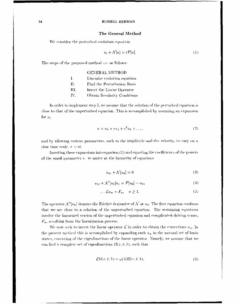
54 RUSSELL HERMAN

The Getterai Method

WVe c01151(ler t he pert l11Ibe( evollit iou eqlatlioll

iut +.1) =la] P[111. (1)

The steps of the proposed method ;i-' as follows:

GENERAL MNETHOD

L. Linecarize evolution equationl

HI. Finid the Perturbttoion Basis

Ill. invert. the Llinear Operator

IV. Oh 4ai Secularity Conlditionis

Iii order tok iiiijikmeuit step 1, w(' assullil( that thli solituozi of the pert irh-e(I ujiiat iou IS

close to that of the luimpertutbed ('(jiat ioi. This is accolniplishecl by wssliniuug all expallsioul

for it,

11 = u + U0 j is I + f 2 & -j-. (2)

anid by allowinig various parameters. such as the atmlphitude anld the Vehwiotv. to varv onl a

slow tine scale, -r = f.

Inisertling these expanisions inito equationi (1) mlid equat-ing the coefficiellts (if e~je powers

of the small parameter f, ve arrive at the hierarchy of ('(quat jolls

"iof + A:'[i.a] = 0 (3)

lilt 4 ' oII11 = P [11()] - n (4)

....-Cufl= F,, , a>. (3ý)

The operatorA`1u() denlotes the Fri~chet derivative of V at un. The first vqilatioii cotifirm.s

that we are, close to a. solutioni of the unperturbed equationi. The remrainiiuig equatiolis

involve the linearized versioni of the unlperturbed equationi and( comuplicat ed drivi I g t ermus.

F, resulting from the linearization process.

XVe, now seek to invert the liniear operator C lin ordler to obtaini the correctiows1 it,, Ill

the Ipr(se1 liet hod'll)( this is accomiplishied by exp)an(ling each u,, ill the( niatural set of basis

states, conlsisting~f of the eigeinfmiuitions of ther linevar oplerator. N aircly, we a~ssume thlat. we

can find a complletc, set of e~igedmfuct ions Q(x, ti A), such that

LAX PAIRS. RECI RSION OPERATORS AND) NONLINEAR EVOLU TION EQU ALIIONS 55

and thant tlicv saisfy ort~li~ogI1tYil relattion' With t1e al(ljoiiit lbasis of 11W form":

< Q(x, t; A )IS ?" I,t ) > Sj I (x, f: A) )At (., I; A')

=- N ý A -'). (7)

1-laying comnpleted step 11 Ne( now carry out step~ Ill by expandling u, as

it, (.r t) /f(A, 0)~x 1 A) d1A.(S

whereI C' is ;III app)ropriat e 'ont our. Operatinig oil (8) WithI C. We o t aim fromi eymlit i n ( 5):

F,= Jf lf,(A.1) Jt~ ~Xt1x A) d/A. (9)

Mil~tiplying hy t he adljoiuit anid integrating over .r gives"

[f,,,(A. t) + c(A)f,,(A, t)[ . < F,,j ýý "(sr. tA) > 0N(A) ()

SolvIIing for f,, ( A, t ). gi vený f, ( A. 0) . we ca 11 writec oi t thI e sohlI t ion for 11

It niav h1appen that oirl sollutii is not lbotnde(I inl tinie. However, froni tit In'i t rodlt m

ijoli of thle slow tillie scale. we use tw lie nknown t inet depenih'nce of ou ur free 1puram netf-ers

to ('lillljililt C t Itt secuillari ties ill tiiiie. Ill thew studyt l of solitomiP(1 prurbatit ons, thlese' cctilarityv

rconditionls det t'xinine11 the solitoxi shape mid velocity.

The Role of Recursion Operators

The key to caiirrying out such anl analysis Is the ability to find the pe(rtuirbat ion basis"

anld the wdj( ilit states, ais w~ell as to prove that fthe ba'sis i's comnplete inl Some sinmi~ abeSpace

and satisifes the orthlogoniality relat ionls inl eqamat ion (7). These queistionls cami be answered

b" uirinug to the the(ory, of rectulsa m operatots. or St rollg syrimiet ries. which we now sketclh

12.13., 17, 19].

IN'- ~ist~j1!. , Lila ( uapcr(tiaurbeti) evolit ionl equatiori

ut + A;'[11 = 0. ( 11 )

The assi ieiate(l liulearize (lqima tion i cali be wriit tel aIs

r,= -A'uJ'.(12)

where previoiusly ',vt had dlefinied ;\ [?i in (4).

Now. ?1 Mr '[(/I is 'A svimietrv of equa11tionl (i11) if

A"II4il- M..'[u1AIN[u1= 0 (1I3)

56 RUSSELL HERMAN

for all solutions u of (11). In particular. tit = Du is a trivial symmetry, where D - (.9Other synumetries of (11) canl be geueratted from the trivial syminetry through the use

of a recursion operator, RIu], of the form [191

R[-] = ,[u]D"' + p- [a]D"-' +... + a0(t] + (_ 1 [lJ[- + + ._.,[j[Dm. (14)

Namely. if

Ru], = [R[uJ. N'[u], 15)

for all solutions u of equation (11). then for every ii > O, it = (R[u[)"Du is a symnletry

of equation (11).

Not e that equation (15) is in the form of zi Lax equatioll. Nanlely, this equation resullts

as a consistency condition for the Lax pair

R[u]o = 7(A)O (, = -N'[t,]o. (16)

In other words, the recursion operator gives the spectral problem and the time evolutionis governed by the linearized operator. Thus, the eigenfivctions of the linearized operator

C are the same as those for the recursion operator.

Furthermore, if we know the ordinary Lax pair for the given nonlinear evolutionequation, we can write the eigenfinctions of the linearized oIperator in terms of the eigen-

functions of the standard associated spectral problem. Assuming that the standard Lax

pair is given by

Lt",• = 0 1t = AR'.'i, (17)

we seek a tralnsformation 0 T(44', A) between the time evolution equations for t. and 0.

Now. inserting u, - T- (O. A) into the spectral problem in (17) we obtain the recursion

operator in (16).

As an examplie. we consider the KdV equation. The well kinown Lax pair for the KdV

equation is given by [Il

D 2 ?,,, + (,1 + A2)1, = 0

?;, = -D'Y I " - 3(u - A2)Dt.. (181

The linearized (quation is found as

t= -D 3o - 6uDO - 6?i& (19)

It c'an he shown that 0 = (D-' /')/'I will transform the time evolution equation in (18)

to the linearized equation (19). Transforming the spectral part of the Lax pair and using

(16) yields the desired re'cursion operator:

Rf,] = D 2 + 4u + 2uD-•1 Y(A) = -4A 2 . (20)

LAX PAIRS, RECURSION OPERATORS AND NONLINEAR EVOLUTI()N EQUATIO)NS 57

Therefore, for the perturbation theory for the KR(1V quatiou. the lperturbation basis

consists of tile states

Q(x, t; A) = ,(,r, t; A) = D(& 2(x, t; A)). (21)

Actually, after selecting tihe correct contour in (8), onie finds that the resi(ues lead 11s to

include several bound state eigenfiictions, {jQj(.r, t), Ak( x, t)}, whose form can -b found in

[5]. Sacis ha.s shown that this basis is complete over the space of contimuous, L' functions,

providing that u0 is bounded in the Sobelev L' norm 118]. The proof relies on the the use of

the recursion operator, though it is not referred to as such. The orthogonality relations can

also be obtained using the recursion operator, though Newell has shown how to compute

these from the spectral problem [16].

Application: KdV Equation

As an example of how this method works, we consider solving the perturbed KdV

problem

Ut + 6?m, + u(F1 -

u(x, 0) = 212sech 2rT.r. (22)

We assume an asymptotic expansion of the form

n(x,t) = ufl(r. t) + (U](X,t) +

uo(x,t) = 2q2 sech 2 7(x- - - x )1 (23)

introduce the time scales T = t, 7 = dt, and allow the soliton paraneters q, x.o, an(d x 1 to

depend on the slow time scale r.

Inserting the above exI)ansions, we find that the lowest order equation is satisfied if

xO, = 47'j. The first order equation is

l = -4?pjrj, - 2rqj,(vO + 2' 3 x, •vo + F[u0] =, (24)

where £ is the linearized KdV operator:

=--OT -- 410 + 6Tqto + 7j0O, (25)

all] 1, =secl¢, e = tl(x - -.xr - ,r1 ).

Our ain now is to invert £til = . We expand ui in the basis found in the last sect ion:

S / dAf(A, t)Q(.r, t: A) + .fl(t)Ql(x,t) + .ql ()A(,r, t). (26)

58 RUSSELL HERMAN

Operating on ul with C and solving for the expwision coefficients, We find

f(A,,t) = f( +Oh 8'A:t ± ______) szA'(t-t (27)a t 2,iAdl(A)

gi(t) = gi(0)csi' - i11) ( ] ;}"''' ' (28)

.fl (t) flt (0 - 4SI,12 tgl(0)f 2ii; j 9it,(11-IAi 5?)J(t

--96rj/ 3 i,'! '(•,i)8'~-') (29)

Using the explicit forms for the eigenfinictions [5], we can write out the solution ofour perturbed equation to first order in t. However, if we write out the last two terms , f

o . we have for B f •1Q + 9gA 1 ,

B = j [sech2+>)h ] + h+ (secl2 i , (30)

where

.0

h .1, d'(.F][6 + 81'3(t - t')]sech 2&2 + tanh p). (31)

When the imner products are time inideplendent, " ,wh is the case for many perturbations.

these coefficients will grow in time. This leads to an unbounded solution. We can eliminate

such secular behavior by requiring that

(F.sech 2 o) = 0 (-Fl6sech'2 6 + tanh o) 0. (32)

Inserting the driiving terms from equation (24) into (32), we obtain the time dependence

of the soliton parameters:

I7 f F[ulistchit 0 d5-oc

1r F[uj][Osech'20 + tanh 6t d6. (33)

The correction in (26) no1W becomes

f<' .o [• tir 'T(.;I')QA(.r.t': A)

-- ( 2 t• 27ri\a (12 ( A t; A). (34)

From an asymptot ic analysis of this integral, we find that there is a decaying oscillatory tailplus shelf behind the soliton [3.5,11,16]. The size of this shelf, which is due to a singularity

LAX PAIRS, RECURSION OPERAF(ORS AN!) NONLINFAR EV(O)LI.UTION [QIIAlit()NS 59

at A 0. can he estimite,,d aits [i11]

Shelves generally occur for d(issila tivye pert tubations. iII which case omli has to o(l)taiin

information frlom the second order iII the perturbation tb,,ory. Doinig his one finds that a

correction to tle soliton shift has to be mahde. Nanily, we obtain )3.3.6.1 11

"t 1, = 4 q-'t Ft][ose"h'o + tanh 0 ± tanh- o] do. (36)

Co1clusion

W\e have seei, a sket ch of t lie proposed miethod applied to the p)ert urbed KdV c(luat 1(n1,

Results have bheen found for a varity vof specific pert urbat ions., leading to previous results.

as w(ell as producing some new ones [3,11,14]. Examples of such st tidies include the damped

[5] and stociastic Kd(l\ [4] eqtmations. WC have also .,,('d these results to study th(le effects

of truication errors in dis(cretizations of the KdV equiation [9].

O)the(r cqulations which have been investigated are thie sine-Gordon [3]. thme n<onlinvar

Schr6dinger (NLS) [5], the( d(erivative NLS. the coupled NLS, tihe Toda lattice j8. andevolution equations supporting loop solitons. An indication of how this methotd can be

carried out for the Kadomtsev-Ptviasl~vili equation was given in [7].

The method discussed here is a natural approach to perturbation sti(dies of soliton

dynanmics. which is similar to methods seen in other works [10,13.161. On(, of the uses of

such an approach is to obtain more details about the' first or(der correction term. This

is important when the growth of the oscillations can have adverse effects (in the systei,

tnder study. such as thle study oif dynamics under random perturbations, or the effectsof discretization error in nunierical simulat ions of thles(,, e(quaiions. There are many other

e(quations. p)ossessing Lax Pairs and recursion operat(ors. whic-h still need to he studi(e'd for

tlh."ir )-ijavivor muider pcrturbiations. In such cases this method woul(d be appropriate.

References

[1] Ablowitz .1 , and Setgur H 1981 Solitonm and thr, Inverrv Sratitcrinq Tranqform,

(Philadelphia: SIAM).

[2] Fokas A S 1987 Symmetries and Integrability. Stud. Appl. Math. 77) p 253-299.

[3) Herman Ri L 1990 Resolution of the motiion tf a pert urbed KdV soliton, In,,r.,',c

Problem., 6 p) 43-54.

[41 Herrman R L 1990 The Stochastic. Damped KdtV Equation. ,J. Phy.,. A. 23 1) 1063-

1084.

60 RUSSELL HERMAN

[5] Hermani R 1, 1990 A Direct Approach to Stmdying Solitoti Pe't urhat ion i'.J. Phy tp. A,23 1) 2327-2362.

[6] Hermixia R L 1990 0 inservat~ion Lawvs and ft(e Pertuinbo(l Kd V Lqjuailtifii. .1. Ph y,ý. A.

23 1) 471947-24.

371 Herman R L 1991 Evohit io -in'f A Nioditdatced NP Soultoil .JPhyo. A. 24 1, 1 161 1 S184

181 Hermani 1 L 1991 The Pertutrbed Todla L.attice. i vpie)ltlt.

[9] Herman~u R L and IKnickerbork-er C .1 1990i Ntiiiirically Inditced Phav,-i Shift In t h"

dXSo~lton 1. stihtiittedI to .1. ClOrnp. Plop.

I il lint) K aind 1c-Iiikaw~vi Y 1982 Lax Pair O)perators for Squared( Eincllfixrict ionl Iin ftw

lInverse Seattierixig Traliiforwitl Ja in ~.. Plh ,p. Sor. Ip vi. 51 1, 40)91

(111 Kar-pullall V I and1( Nlaslov E. M 1978 Structurtil of TllV Prodiweil findle ft(li Actlonl of

Pert i rba tiojis of So litons Sov. PhY.t1 . J ETP 48 p) 232 25S.

j12] IKatp D .1 1983 Thiermial Correct.olls, to (iverdalinped Sob toit Mo t ionu Phy!P. Rev, B.127

1) 67 87T- 67T95.

[131, Kaupi D) J and Ne-well A C 1978 Solitojis a., Parlicides, ()sejH;, tois. anld Iil SlowNl v

Changing Media: A Singubar Pertulrbatio 111fliqry) Proc. Roy. Soc. Lond. A361 ip

413-446.

t14] Keeler .1 P ;tid Mcf~i igtliii 1) W 1977 Solia ons Utoler Pertm1)i (h i tol Ph p. ut v A 16

p) 777 7901.

i151 lNoni-ocaictlilko 13 G~ 1987 Aonihrifar Intfcqmhlv Etjtu, iom, Let ire Notes Minyc

No, 2 -40, Springer Verlag, Netv York).

I6'j Newell A C 19.S()rii Tue lversf Scatterjing Trballsforult In Sollton-q. vd. l3'illoiigli P K a'ld

Caiidr-e P J1 (5pringer- Verlag. New York) p) 1 77.2942(173 0Over P .1 1986) Applicof ov.4 of L c Groap.q to Dfrir.ti Jthuru.(M No. ]0'-7

Sprngr-ei ~g.New Yo rk).

118, Swch" 1? 1, 19.S. (ozlitjdetins, of PDivaIv;fv,-s of Square'l Selir"Ainge, ijt'fiein

;w xpii S, dt ioil' of fthe Lmicitrized XdkrI Eqjimt ion S1I4AM 1. Moth. A 71(1. 14 p)

671 6')3.

13193 St ralitpj NV 198 Lx Pis Spcct ial wiilii.ad TRectýsuril 0 )pra;trxz IMI 25 P)

290.7) 2909.

12013 XVasIjtijii 11 mnid Tmlt] 'iI.196G; Piop~ja;itiotl of loil weolltic Solitary ave' of Sniol1

Anipli iili. 111op. R'iv. bs 0. 17 P) 99 9

The Depart. mienti of Mathematical Scienceslhiiiversity of North C~arolina at Wilinhiigtoix

Wilminiigt on, NC 28,403-3297

Conitemptriry ah. ti.

Volume 122, 1991

Time and Temperature Dependent Correlation Function

of Impenetrable Bose Gas Field Correlator

in the Impenetrable Bose Gas

A.R. Its

A.G. Izergin

V.E Korepin

Abstract

Asymptotics of the temperature time-dependent two-point field correlator

of two fields for one-dimensional bosons with infinite point-like repulsion is

calculated.

1 IntroductionAsymptotics of temperature time-dependent correlation functions of impen-

etrable Bose gas are given in this paper. The Hamiltonian of this quantum

integrable model [1] is

II = J dz(O&(k+Ozt + c¢+'4, - (1)

with coupling constant c = +o(. Fields ?p, 0+ are canonical Bose fields

IP), MIfalhtnaru.s Nubhctf ('lassts'watton 82A 5.This paper is in final form and no version of it will be submitted ror publication elsewhere.

(i) 1991 Anwrican Mitii itati'al Soci•'ty0271-41132/91 $1.00 lU S .25 ptr pagi,

61

62 A. R. ITS, A. G. IZERGIN, AND V. F. KOREPIN

in one space dimension, i.e.

[¢(z1 , t), 0+(z2, t)] = 6(z1 - z2). (2)

Thermodynamics of the model was constructed in [2]. The chemical po-

tential h defines the gas density D. At temperature T > 0, D --+ 0 as

h -- -o and D -i o: as h - +oo. In the state of the thermodynamic equi-

librium the distribution of gas particles (possessing momenta k and energies

e(k) = k2 - h) is given by the Fermi weight p(k)

p(k) = 1 fk h W- 27r(l+exp{ T00

D = p(k) dk. (3)_ 0

Professor C.N. Yang drew our attention to the problem of the calculation

of time and space dependent correlation functions at finite temperature.

The two point field correlator considered is defined as usual by

tr(exp{-H/T}O(z2, t2)0+(Z1,'t1))(4

< 4'(z2, t2)0+V(zi,t1) >T = tr(exp{-H/T}) (4)

The equal-time (t, = t2) temperature correlator was completely described

in papers [3-5) where the integrable partial differential equations for it were

derived and asymptotics in various regimes was obtained (for zero-temperature

equal-time correlator it was done earlier in paper [6]). It should be noted

that the starting point for consideration in papers [3-6] was the represen-

tation of the equal-time correlator as the first Fredholm minor of a linear

integral operator [7].

The analogous representation for time-dependent correlator (4) was giv-

en in [8], which was used in [9] to derive integrable differential equations

CORRELATION FUNCTION OF IMPENETRABLE BOSE GAS FIELD CORRELATOR 63

that completely describing the time-dependent correlator. These results are

briefly discussed in the next Section.

2 Correlator in terms of Fredholm determi-nant

Correlator (4) depends essentially only on the rescaled variables1 1

X - (z, - z2)VIT;t =_ -(t2 - tl)T; 13 =- h/T (5)2 2

which can be easily established using the representation of paper [8]. So

one has

< 7,(Z2, t2)0+(ZI,,tI) >T=--VT g(X, t, ý3). (6)

For g one has [8,9]

g(X1 t, 3) exp{2it13}b++det(I + VT) (7)2-,r

where the Fredholm determinant of the linear integral operator VT acting on

the whole real axis enters the right hand side. The kernel of this operator is

VT(A, i) = (A - y)-'[e+(A)e_(p) - e+(j)e_(g)], (8)

with

C_(A) (A) exp{itA2 + iZxA,7r

+(A) = e-(A) E (A),

E(A) = f_ CxP f ep{-2iWt- 2ixv}. (9)

The rescalcd I-'crmi weight 0(A) is

o(A) = (I + exp{•A2 - /})'. (10)

64 A. R. ITS, A. G. IZERGIN, AND V. E KOREPIN

Function b++ in (7) is defined as

b++ -B++ -G,

G j dut exp{-2ity' - 2ixp)}. (11)

"Potential B++ is cnc of tO.he potentials B,., Cjk(i, k = ±. -):

Bik = J ej()fk(As)dp.;

f00Cik = f 0iej(p)fk(pi)dA.,

B+_ = B_+, (12)

where functions f± are the solutions of equations

f±(A) +± VT(A, p)f+(f±)dl = e+(A) (13)

3 Differential equations for correlator

Let us define a vector function f:

f(A)= (f+(A)) (14)

Differentiating (13) with respect to x, t and applying operator (2A&O+Ox)(this

is done similarly to the equal-time case [3-51) one obtains a Lax representation

L(A)f= 0, M(A)f= 0, N(A)f = 0 (15)

with

L(A) = a, + i•Aa3 - 2iQ,

M(A) = -iO, + A20 3 - 2AQ - V,

N(A) = 2U0 + Ox +2iAta 3 + ixa 3 -4itQ - 2&oU, (16)

CORRELATION FUNCTION OF IMPENETRABLE BOSE GAS FIELD (ORRELATOR 65

with

Q (0 b++)

( 2b++B__ 0O, b++)V = -iOB__ - 2B__b++

U = ( B+_ b++ )

-B__ B+_ .

All the operators L(A), M(A), N(A) should commute at arbitrary value of

spectral parameter A, which lead to nonlinear differential equations for po-

tentials Bik. Introducing notations

g_ = exp{-2i1t} B__; g+ = exp{2itz3}b++,

n - g+g_ ; p = g-_r+-g+i- g+ (17)

one obtains first of all the separated nonlinear Schr6dinger equations= 1

-i(,,g+ = 20g+ + 1-&ýg+ + 4g'g_2

1+iOtg_ = +208 g- + 9O.g_ + 4g9g +

-2i,9tn = axP (18)

Equations containing the 3 derivative are

=0 0.o+ _ 0,00 -o - :E (x,t,/ ) (19)9+ 9-

(new function 0 is defined here) and

-ia + 490•p = 0

0•O+q8aon+2 = 0 (20)

This is a complete set of equations for potentials b++(B++) and B_. Initial

data at t = 0 for these equations can be extracted from equal-time correlator

g(x, t = 0,13) g(x, 03) completely described in [4,5]. Other potentials B,C

66 A. R. ITS, A. G. IZERGIN, AND V. E. KOREPIN

(12) are defined in terms of these two. Namely,

a,:B+- = 2in ; atB+- = -p;

aoB+- = ix i(21)2 4-

and

C++ = O.B++ + B++B+_ - 2GB+_2

C__ = - .OrB_ - B+_B__

.(C+_ + C-+) = (B++-2G)8XB__ - B_.-& B++ (22)

Correlator (6),(7) is essentially a products of potential g+(17) and exp{a},

o = In det(I + VT)

It is easy to get an equation involving only g+ expressing from the first of

equations (18)

1 2 -g9 = -( - 2iatg+ - 406g+ ±,O.g+)g+i (23)

8

and substituting this expression in remaining equations (18)-(20). At t = 0

function a is known [4,5]. The derivatives of a can be expressed in terms of

potentials B,C as follows

0-,=a -2iB+- ,

DOa= -2iGB__ - 2i(C+- + C-+)

000 = -2itOO(C+_ + C-+) - 2ixO3B+_ - 2itB__O.9B++ +

+ 2it(B++ - 2G)8OB-- + 2(aOB++)(8eB__) - 2(0tB+_). (24)

(the calculation of (9,9a is not very straightforward; it is done analogously to

CORRELATION FUNCTION OF IMPENETRABLE BOSE OAS FIELD (ORRI•VI(TOR 67

the corresponding calculation in the equal-time case [4]). This completely

defines the correlation function.

4 Matrix Riemann Problem

The most interesting from the point of view of physics is the asymptotic

behavior of correlation functions at large time and distance. As in the equal-

time case [3,5], it can be calculated using the matrix Riemann problem of the

inverse scattering method for classical integrable equations (18)-(20) describ-

ing the correlator. Consider the matrix Riemann problem for 2x2 matrix-

valued function X(A)(detX(A) 0 0) which is holomorphic for ImrA > 0 and

ImA < 0, and equal to the unit matrix I at A = oo, X(oo) =I. The boundary

values on the real axis are related as

x-(A) = x(A)G(A) (25)

The conjugating matrix is

-e+(A)e_(A) e 2(AX) (6G(A) = I +2~ri ( _e_(A) (A) A)e(A)

with functions e±(A) just the same as given in (9). In complete analogy

with the equal-time case [5) one can show that the standard singular integral

equations for this Riemanjn problem are equivalent to integral equations (13),

the solutions f±(A) being simply expressed in terms of X(A), namely,

( f+(A) '\ -(A) e+( A (27)f_(A) ) e_(A) )

Potentials B,C (12) are then readily extracted from the (1/A)-expansion at

A -*oc:

X(A) =I + (TI'/A) + (lk2 /A 2) +...,

68 A. R. ITS. A. G. IZERGIN, AND V. E. KOREPIN

•1 = -B_,B+_ ; = -+_, C++ (28)

The calculation of asymptotics of the potentials at x -- o0, t 00 is

similar to the simpler case x -- 00, t = 0 [5]. Nevertheless there are essential

difficulties due to the appearance of stationary phase point in the singular

integral equations. Using then partial differential equations (18)-(24), one

restores the asymptotics of correlator (4)-(7). The derivation and complete

answers will be given in more detailed paper. Below the first results are

formulated. It should be emphasized, however, that our approach gives a

systematic method to calculate the asymptotic expansion (see[5]).

5 Asymptotics

Consider first the case of negative chemical potential (h < 0). In this region

we obtained the following expression for the main term of the asymptotics

of correlator (4)-(7):

< ý)(z2, t2)ý+(zht1) >T=

2 ia

avfT(4t) 2 exp{2it/3 + 2-} x2t

x exp{- x + 2pt In (,2- +

1 ,1 t

(x - (_ - Z2)vrT; t = -(t.2- tl)T;2 2

0 =(h!T) < 0; x- +oo, t --- +o) (29)

Herev -In V -

7r exp{( )2 -t } -I

and coefficient a depends on ý3 and the ratio (x/t) only. We would like to

(ORRELATION FUNCTION OF IMPENETRABLE BOSE GAS FIELD CORRELATOR 69

emphasize that G.G. Varzugin took part in derivation of (29). The expression

for the coefficient a in (29) is complicated. To write it down let us introduce

the following notationsA = I 2+1

2t 0nýb r (V sin(A - )Ioo-A17I 0 (e--ll d

(30)

Now coefficient a in (29) can be represented as1~ {IV) .+ V_2

ev - (exp 2 -)+iko+0 -1 2 (i+ +-)di+

4 22i- 0 2+ J -I: _00 dp sin(p - Ao~ln +IdP3 (31)

It is interesting to compare (29) with the result for the equal-time corre-

lator obtained earlier [3,5]:

< V)(%ý2, o)V+(Z1,, ) >T=

= V/Iao (/)exp{-x(2•j -+ c(P))}1

(x - (Z2 -z 2 )v/ -- + o, 1 = hIT < 0) (32)2

with

0) 0) dp In lexp{l' - 0} + 1 (33)7) f 00 lexp{jI-/3}-I

and

a(o(13) I0 exp 1- _ 11/2 0o dU In _______+I X101/1 r Joo A \exp{l2y - 0} - I)X exp{i f -dr7 dc(T)

(Po is a constant).

70 A. R. ITS, A. G. IZERGIN. AND V. E. KOREPIN

For positive chemical potention (h > 0) one obtains

< )(z2, t2)0+(Z1, t1) >-r=

= aVk(4t)"' 2 exp 00 + 2pt Iln - dy + 0heAr e 2-0 --

I - hX 2(Z- IZ2)VI,,,-t 2 2 (t- t,)T; o= > 0

2= > 0;-x +• 0- t -+ +00) (34)

This is in agreement with the previously obtained answer for the equal-time

correlator[3,5]:

< O(Z2,O)V)+(z1,O) >T=

Po p 0 -exp - I drt dCr) ) 2jexp{-XC(13))

X I - z2 )' - +oo,/ --- - ) (35)

Here function c(fl) is given in (33) and p. is a constant of paper [10]

(pOO = 7re-1/ 22-1/ 3 A-6 , A being the Glaisher constant).

Acknowledgement.s

We thank L.D. Faddeev and C.N. Yang for helpful discussions. This pa-

per was supported partially by the National Science Poundation Grant No.

PHYS9-O08195.

REFERENCES

1. Mathematical Physics in One Dimension, Eds. E.H. Lieb and D.L.

Mattis (Academic Press, New York 1966).

CORRELATION FUNCTION OF IMPENETRABLE BOSE GAS FIELD CORRELA.FOR 71

2. Yang C.N. and Yang C.P. Thermodynamics of a one-dimensional sys-

tem of bosons with repulsive delta-function interaction, J. Math. Phys.

10, 115-1122 (1969).

3. Its A.R., Izergin A.G., Korepin V.E. Correlation radius for one-dimensional

impenetrable bosons, ICTP, preprint IC/89/107, May 1989, accepted

to CMP.

4. Its A.R., Izergin A.G., Korepin V.E. Temperature correlators of the im-

penetrable Bose gas as an integrable system, ICTP, preprint IC/89/120,

June 1989, to appear in CMP.

5. Its A.R., Izergin A.G., Korepin V.E. Long distance asymptotics of

temperature correlators of the impenetrable Bose gas, ICTP, preprint

IC/89/139, June 1989, to appear in CMP.

6. Jimbo A., Miwa T., .M6ri Y., Sato, M. Density matrix of an impenetra-

ble Bose gas and the fifth Painlev6 transcendent, Physica ID, 80-158

(1980).

7. Lenard A. One-dimensional impenetrable bosons in thermal equilibri-

um, J. Math. Phys. L 1268-1272 (1965).

72 A. R. ITS, A. G. IZERGIN. AND V. E. KOREPIN

8. Korepin V.E., Slavnov N.A. The time dependent correlation function of

an impenetrable Bose gas a a Fredholm minor. I. Preprint CMA-R28-

29, Australian National Univ., Canberra, July 1989, to appear in CMP.

9. Its A.R., Izergin A.G., Korepin V.E., Slavnov N.A. Differential equa-

tions f-br quantum correlation functions, Preprint CMA-R26-89, Aus-

tralian National Univ., Canberra, July 1989, to appear in Journal of

Modern Phys. B.

10. Vaiya H.G., Tracy C.A. One-particle reduced density matrix of impen-

etrable bosons in one dimension at zero temperature, J. Math. Phys.

20, 2291-2303 (1979).

Leningrad University, Leningrad, USSR

Leningrad Branch of V.A. Steklov MathematicalInstitute, Fontanka 27, 191011 Leningrad, USSR

Institute for Theoretical PhysicsState University of New York at Stony Brook

Stony Brook, NY 11794-3840

Coit ein pi orar' N it t I ~irei t ic

\oljit, 122. 1991

Breathers and the sine-Gordon Equation.

Satyanad Kichenassamy

1 Introduction.

Thl purpose of this paper is to report on a recent non-existence result forbreather solutions of nonlinear Klein-Gordon equations [1.2]. and to mentionsome technical improvements thereof.

One of the by-products of the method of Inverse Scattering to solve nonlinearevolution equations is the construction of the "breather" solutions of the sine-Gordon equation

Utt - UXX + Sill d = 0. (1)

The simplest of them is a periodic solution, with period 2r/1rl - c2 (0 <

E < 1) which tends to zero as Ijx -Yx-: it is given by

ls, = 4arctan E - os(t " (2)USG kr _/jT.2 CoshL1 e (2

This solution, which can be inade arbitrarily small in. say. the L2 norm.by taking the parameter E sufficiently small, has remarkable properties. thatare shared neither by solutions of the (linear) Klein-Gordon equation, nor bythose of other soliton equations which. like the Korteweg-de Vries equation. arerelated to a self-adjoint eigenvalue probhlem. We will not detail these propertieshere.

Solutions with behavior analogous to that of (2) have not beet found inother equations of the form:

1te - Ux. + U1+ ±(UL) = 0. (3)

"School of Mathematics. 226 Vincent Hall. 206 Church Stret S. E., Minneapolis. MN 55455;work partially supported by an Army grant

1991 .amh•fattao Stdiect (Tlassrlwm,'a. 35L70. 35BM 3513B25. 35Q20.This paper is in final form and no version of it will he submie'ed for publication elsewhere.

Q 11991 American Mathematical Socitcty

0271-41132/91 $1.00 + $,25 ipr pag'

73

74 S.-TY AN.-X) KICHEN ASS.AMY

with 1 Y( i) = gJ2 it + g3ld + -- I aittI t his leads to( the pst itVthat breat hertsmight he specific to comlpletelY int egrable Slyst elis.

The two qjuest ions 'ofore uts are t here-fore:

1. \V\ixtt shiould( he calledl a blvwIater soxlutiion of ~i et-ut egral ave qua-

2. Do such solutit ons ex ist for (3)?

\\e here ýsuliinllarn'e. withI a fewo addfirion>-. the ans"wer>- top h11-w quest Ii' itigivenl ill f11 briefiy tt~nuleft'lt onl their prVoof", 611!2 and ~its Stim iiprove-

intt inl ý3. (A discu-ssion (if t he Ilitera!ture ott Ithis Jpro~ihll't calfit,1 faxtid I'lJIiof ;1.

A.: breather is a timue p)eriodlic solut!ion of (3) which (hca ,vs it) zrn) a>ý xg~oes to infillitv. (This. definuit ion is dliscuissedi and ext ended in) IT')

2. There are f rxtual breathers:

if III Ex~(. t\1- 2 £u2 (£r FV 2 .

for (3). chtarac'teriz/ed by Iperjodicit V. decaY and parity condit ions, if and(only if

:3. If series (4) defines a soltut ion of (3) analv N-ic Inl an ý ýd fV'j -2 for

-c1< 4-, ,Ufo an. r > 0 aI](t sly!' x. (loseý to thne real iixis,. andv'2

if this funct ion hias- all expatision inl potwers of e ~~and Fo(tVI-£uonver-gent for large x. then tu + y H) =t So-1 s 0l(oa. (Inl thisý caste,

,eries does have thle assert ed analyt icitv" proprt v

1. If q is odd. anl

11w, < (1111-111m!frsomle (t > 0, t hen eq. (3) does hiave a time periodic sobtltion on some

iinterval (A. + x aiven byi a powe r scr ies inl conive rgen t for tr arge, ian sTilall £. This soluitionl is the tollk otie whilch isodd inl cosft

and tend> to zero exjpotenttiallv as xr tends to ± x,

1? works,: I. W\e have thus aeilievc'd a ('Itara-te'rizat iol (of the Sinle-Gordioneqpuatol ;mu mon nonlinear Nlein-(;ordlon eq~uat ions. This I.is a rite~ri(tti for coot-pletc inltegrabilitY of ý31 via Ifthe Zakhiarov-Sliabat eigerivaluet pt-Odtexuc

2. T h t- intrabilit v liren orre!,ponds, to a sumot~hites, properlY o)f 'pecal

3. 'I'll ("\I-Crgc 1 ncef re lt i1ili odd came tiss ifiest ilie pert tttlat i'1 approit;1tltakeni litre; Tfiere Is, a natorail caxididatt fobr a 1laeat her for every -niall -. utl itib ricvtr antalvt it except inIII tht egvoralh cli as.

1. Tlit tcoistrlutioli ()f Hthe first form11al sohltt on od couse i-w alcpr)Xhmniltt

:reatfr her-Owthi anY dcsi ret I re-;Ptc 0.

BR[EATFIHERS AND THE SINE-(ORDON EQUATIO )N 75

2 Sketch of proofs.

The proofs are based on the existence. for very general functions y. of twoformal periodic solutions of (3). We first introduce a paraielt(,r ý" and twoscaled variables ý and r by

E=X.7 = tV -C 2 .

and lett = Fr. Eqtuation (3) tlheni oic(oliles:

r,, + ' - T2(uii + U,-,) + q(,v)iE = 0,

and we seek v, periodic in r with period 27r. tending to zero as ý goes to -±-x.We also Ypect iu to( depend smoothly on E, as in (2). The corresponding a willth(len b)e called a breather solution of (3).

The first formal solution is in increasing powers of s:

Zu = E k r). 7)-

We assume Uk has the same properties as it. If the Ilk are even in l and r.they can be uniquely determined by from ui. On the other hand, if i t 0. thenwe must have:

ul = +± Acs•- COS

where A = 5g.2/6 - 3g 3 /4 must be positive: otherwise formal breathers do notexist.

The seconu formal solution is in increasing powers of c•-:

-kýl11 Ze k -(~r). 7)

We again take I', even in r. This series is determined by its first term, I-,. whichiust have thle form a(g) cos r. No condit ion on g similar to (5) is required here.

The existence of the first formal solution prowves slatemenllt 2. in the ilnro-

duct ion."TIo p)rove 3.. one shows that if i had the given analyticily propert-, then it

would have an (lexpansion of ty.,pe (6) which (couhl Ib' rearranged ill the fori )with coeflicieints holowiiorphiic il r for ýý! < - + (ý. O)ne then proves. using the

analyticitiy again. that a(•) is always, no nzero. so that after a translat ion in l.One mI , asslllml(e (ý) 1. ()nle ne('Xt Prov's b)Y inidu'tioin thait the ?'k n (ssesspole's which approachw 0 as k increases, and that all the poles of i•iodtihlus< 1 i/v'2 disalppear if and oilly if !( n) I= o-, sin( mo). (k-o siih(l n ). or i. oillV

ie(, first of th ese giving rise to breathers ais (wne, verifies direct lv."To prove 1.. one Hse" ;I aiajoariut metlhod based oil comiparisonor witl ilie

soluit im of hie sinhr-(Gordon e(quat ion corresponiding to (2). ()ne, ob)tain.s, theun•qu('1iess ,talt ment bYl a variant of tie(' stabl manifold theorrn,

76 SATYANAD KICHENASSAMY

3 Remarks.

1. Because of translation ilnvariance, it is apparenlt ttlat somle Coii(litioll.

similar to tile parity ones uste(d here, is iiee(de in order to fix tihe solutiot l uiderconsideration. ()i the other hand. we next very briefly outlim, a technique whichenables oie to relate the general formal solutions to the even ones.

The idea is this: we know [1] that series (4) is (leterininedf by an ind uctitulwhereby at the kth stop. the hare onics If lk diff('eIt from thd( fI'::-. ,,/ the

first harnionic of Uk-2 arte found. Thiey were uniquely dc'termiliedl because ofthe parity assumptions. Now if we drop these assumptions at soNICe givel '.0epk. we find that Uk and 0

k-2 differ from their values in the "'eveni' case 1 y terillsof the form -m siliT and {,,•-2Sr (with the notation il := S( ') (cosr: ul caniclearly be taken of this form. withi S even. after ain initial translation.) Theobservation is then that replacing ý and7 r by ý - ,,._ 2 n' -2 and T - T-,n¢ .

produces a new formal solition which coincides with the "'evei one it upto order

k inclusive, apart possibly from the first harmonic of uk-, ()ne may carry on

the process by induction.2. The presence of poles iii the expansion (6) Cail he interpreted in terms of

"'resonances" as follows: Considering (3) with periodic conditions inl time define..a d(yinamical system in a space of periodic pairs (u(x. t): ui,(x, t)) with .r playinigthe role if a--tine'" x.,ri'Able, for which orbits hloinoctlimic to the zero solit ioncorrespond to breathers. Now the poles we obtaini here are exactly those forwhich the eigenvahles I and E of this system resonlate with one of the others.(This. incidentally. can happen in the odd case only if E is pure imagtinary.) Theextension of our definition of breathers to other "learl integrable equations."

and more examples of this resonance phenomenon will he given in a paper illpreparation.

3. On(e may ask whetler our emphasis on rapidly decreasing solutions isjustified. Iln this direction, o011 can prove (see [3] for the precise stateriomitand proof) that solutions which decay faster thani 1/,r2 Ilmust have ff( I +X 2 )',u(x. t1 2 dxrdt < x for every ,s > 0. This follows from a general decayresult for linear wave equations. This diliotomy is of course not surprisingwhen compared to similar results for ordinary differential equations.

References

[1 S. Kichienassamny. Breather Solutions of the" .\onluir1r 11ai'rc Equaboin. toappear in Conm. Pure and Appl. Mathi.

[2! Earlier references oii tle subject are givenm in I1].

[31 S. Kichienassarny. Spatial Di'ay of Solntion.s of Li 'ar Wart''f Epi Otf ws.pre print

U.niversity of M innesot a

'(In Iv It4AII -4, lV t hei i W\~i~*122. 1991

Localized solitons for the Ishirnori equation*

B. G;. Kouojwlcheiiko* *

V. G. Diibrovskv

Abstract

The (oherenit strwtuires. for Ohe Isifiniori-Il eýquationl artestudiried. Genewral form of the e!xac-t solutions of the Ishiniori-11(irieqation withi nontrivial bouindaries is found. It is shiownithiat there itxist thef four (e-sseýntially the three) differenittypes (ss. sb). Ihs. 1b1) of localizedl solitons for this equiationlwithi the tinwi-iiid1ependerit )oliin(larieýs.

Onec of tOe rmait features of nonlinear p~artial (liffetrential equiat ~ios

solvab~le 1)y thehinvetrse spfit.etral transform (IST) mel(thiod is the existenicet

of t li localizedl solitonl solu.tionis (seet e,.g. [1-31). In1 the( 2 + 1-dimencisionis

511(11 exponlentially localizedi solitons have beenr constructe(l rcenitly for

the Da~-twirtsoni (DS)-I e(luatioti iii the paper [4]. Scatteýring of

tiliese locafizedl solitonls. their prolpert ics ani(I general initial-l)olliidarv

vabe, Jroblvlen for the DS-1 equlationi have b)(een sttildiedI 1by (liffereiant etIil-

(HIS iij [4-8].

flie pre~seit papier is (levote,(l to t li st iidx of tile localizit(l solitons for

*Talk given at the AMS-IMS-SIAM Conference -I T Li tt);SCattering and( a JppIicaýt icn&''*

Inn" h-12. Amherst. MA. USA19 1i tJUjj iUIOO SIi "ijh , t(fir, w wi u ciun I-SO I iý 150211 w piipcr isý in tinal formi and no %crsiiin of it %M b(l heuhmnitted for Ufiubl(aion ifcse-here

ýi,1991 Aliioricaila loit :0t witv

11271 1:132/ i! IS1 (III) 2.5 1wr pay,,i

77

78 B. G. KONOPELCHENKO AND V. G, DUBROVSKY

the Ishimori equation [9]St(x-y.t) + S X (Sxx + (2Y)+ -xSy+ 2uSX 0.

; - a2 vp + 2(k2 S( S x S , ) = 0 (1)

where S (S 1 , S 2 , S 3 ) is the three-dimensional unit vector

S 2 = 1,y(x.yt)

is a scalar field arid k2 = ±1. Equation (1) is the 2 + 1-ditriensional in-

tegrable generalisation of the Heisenberg ferro-magnet model equation

St + S x S, = 0 (isotropic Landau-Lifshitz equation). The Ishirnori

equation (1) is of the great interest since it is the first example of the

integrable nonlinear spin-one field model on the plane. An important

feature of equation (1) is the existence of the classes of the topologi-

cally nontrivial and nonequivalent solutions which are classi;ied by the

topological charge Q = • ffdxdyS(Sx x S.)[9].

The applicability of the IST method to the Ishimori equation (1) is

based on its equivalence to the commutativity condition [L1 . L 2] = 0 of

the operators [9]

L, = aoy + POx.

L 2 = iOt + 2PO± + (P+PP - i(a3 P + iýýy)O&" (2)

where P--'-S(x.y.t)Or.a = (o 1 ,a 2.,73) are Pauli matrices and 0,-

.ToC = _L),Ot =-!2 The standard initial value problem for theJ• X" -- Oy - at"

Ishiunori-I ((t = i) and Ishirnori-JI (a1 1) equations with the vanishing

bomi(lary valhes ( S - (0. 0, -1). - 0) has been solved in:r . y • "X.,X . y-.)--CT

the papers [10-12] with the use of the 0-nethod ((t = i [10.11]) an(l

nonil'ocal Rieniann-Hilbert problem (i = 1 [12]) method.

LOCALIZE)D SOLITONS FOR THE ISHIMORI EQUATION 79

Here we present the results concerning the construction of the expo-

nentially localized solutions of the Ishinori-II equation with the nontriv-

ial boundaries [13]. In the characteristic coordinates 1 = ½(y + x). 71 =

-_) equation (1) at ck = 1 is equivalent to the equation

- -- " 1 [ . .

St + •S x (S• + S,?I) + 2-( dq'S(S• x S,) + 2U 2 (•,t))S•

- 2( +(, Sn)+2U1 ?(,, t))ST, =0 (3)-- C

due to the equalities

11r/ --. -- ' --.

f= dr'S(S, X S,7,) + 2 2 ([,.t).

<= ]d'S(S4, x S,,) + 2U 1 (r), t) (4)

where U( (q. t) and U2(•. t) are arbitrary scalar functions. So. we are

interesting in the exact solutions of the Ishimori-Il equation with the

boundary values

S(X..Y. t) - (0.0. -1),X2 eg2 -- IX

y(x. y, t) - 20&'U 2 ($. t) + 20,71 U1 (q'. t) (5)

with given functions U1(rj, t) and U2(•, t).

We will use the method proposed by Fokas and Santini for th' DS-I

eqIlation [6-8]. Within the framework of this approach one needs: 1)

to derive the equations which solve the inverse problem for the linear

equatio(n Lj" = 0. associated with the given iritegrable e(quatioun, 2) to

80 B. G. KONOPELCHENKO ANt) V. (i. DUBROVSKY

solve the inverse problem equations for the degenerated inverse problem

data. 3) to construct the modified second auxiliary equation L 2 - j = 0

and to find the corresponding time evolution of the inverse problem data.

4) to construct the exact factorized solutions of the linear evolution

equations for the inverse problem data. 5) using these solutions and

reconstruction formulae for the degenerated data. to calculate the exact

solutions of tie soliton equation with the nontrivial boundaries.

Following this scheme. one gets for the Ishimori-IL equation (3) the

following results [131.

1. The inverse problem equations for the linear auxiliary equation

L,'O = 0 where the operator L 1 is given by (2) are generated by the

corresponding nonlocal Riemann-Hilbert problem [12.13]. Namely tran-

siting to the functions X defined by

( 0. eq (6)l

where A is a complex parameter, one can construct the solutions X+

and V- which are bounded and analytic in the upper (YmA > 0) and

lower (YmA < 0) half-planes. respectively, and such that x+ - at

the real axis (YrnA = 0) is expressed nonlocally via X-. The solution

of this nonlocal Riemann-Hilbert problem is given by the linear integral

e(quat ion

+ Cc

,1.A ) I[ dp dq X -(.,, 1))Z (p. q)±X- ) l+ ri.,I j P- q2 q--x A+)

~~~~~ -)CH lI

LOCALIZED SOLIToNS FOR THE ISHIMORI EQUATION 81

where

e P0

+0, tT'(p. q)f(P.q) = - (p.q), f ,(8)

--OC

and

+CNC

T + (p.q) ((P(ff C ) + 0'3)(O -(0 + -)X+( ,r q))12

T-(p.q) = La +I((P(.ri) +1 )(O +- 0 + )X-(L.,q))21._1 q (9)

The formulae which allow us to reconstruct S and V via X are of the

form

S(,t) = -tr(939

•(,•,t) = 2i logdet g + 20-1U,2((', t) + 20-'U,(rq', t). (10)

where g(, 7t, t) = X(ý. 71. t. A = 0).

The formulae (7) and (10) form the complete set of the equations

which solve the inverse problem for the Ishimori-LI equation. The func-

tions T+(p. q) and T-(p. q) are the inverse problem data [12.13).

2. For the degenerated inverse problem data. i.e.

N,

TI(pq) = Tk(p) tj (q) (11)k=l

where T,ý(p),. T:(q) are arbitrary functions. the inverse problem equa-

tion (7) is reduced to the system of algebraic equations. As a result. the

• • . I I1

82 B. G. KONOPELCHENKO AND) V. G. DUBROVSKY

solution X-(A) is found in the closed explicit form (13]:N_

xyi(A)

(X- (A) o (O\ -7 j A21 ) (1)j=1

- (A)'N+

x (A) } i Z j( j( e y (12)

where+ Dc-+:•Cf(A')

(f(A)):: J dA' f (A )2rri I '- (A ±iO-)

andN- N,

Fj = -A)-' (E a-(TI)T+

k=l R=I

Gj= Z(l B)-1k Z - )r(7)

andN+ N-

= k Zci(?>i() Ber kk=1 k=1

+OC

"r(p) = 1 J dA+

-- OC.

+OC

The formulae (10). (12) give the exact solutions of the Ishimori-lJ equa-

tion which depend on the 2(N±++N_) arbitrary functions of one variable.

3. Nontrivial boundaries (5) demand the modification of the second

onepator L 2 -, L2 + A which is associated with the Ishinmori cquation.

Since the compatibility condition for the system

L I ,=O. (L 2 + A)=0

LOCALIZED SOIUTONS FOR THE ISHIMORI EQI ýATION 83

again should be equivalent to the Ishinori equation, then 01A.4 = 0.

So. the functions 0, and AV) obey the same differential equatiol. But

the corresponding integral equations are different. Comparing them. one

finds [13]

f 02 (iO - )

(13)

where

+OC

y(A) d- J2dr e U2 (&try(A) = -2 dJIUl(7(t)e-•'".

Now, the equation (L2 + A)V) = 0 where L2 is given by (2) and A by

(13) implies that the full Fourier transforms of the inverse problem data

+q + L

T t) if fP• qT+(p q)e P

C Pf d2 dq 2 . _ ,.~

-( 0r,.t) = -i LJ f4qT -(p.q)e v (14)

obey the linear equations [13]

t) -i ,-I +T,:17)+ 2 ý.t)Tý- Ui, (,t) T,7-= 0. (15)

These linear evolution equations for the inverse spectral data play

a fundamental role in the whole of our construction. Emphasize that

equations (15) coincide with the linearized equation (3) for S± --S1 ±+iS 2 .

In the weak field limit one has T±(,1, t) = rS±(ý,r , t).

84 B. G. KONOPELCHENKO AND V. G;. D[URROVSKY

Note also that for the real S one has

qT-(pq) -p(T+(qp))*

or

T (•i, ht) = + , (1)

So. for real S it is sufficient to consider one equation (15), for instance.

the equation for T+. In what follows we will discuss the case of the

real-valued S.

4. Equations (15) admit the separation of variables. So. the equation

for T+ has the solutions of the form

q. t) = 27 E pjXi 0.t)Yj (7. ) (17)i~j

where Pi are arbitrary constants and Xi and Y' obey the equations

iXit + 1 Xi• + iU 2(0 ,t)X,ý 0.

2 - TIT) - iU, (qj. t)Y,= 0. (18)

The inverse problem data T' of the form (17) are degenerated one

ani the corresponding functions Tk-(p).T (q) from (11) are

++:

4- (P. t) = 1-• ,J d T )- • .

Tk -k

Vý, 7ri

LO(CALIZEf) SOLITONS FOR THE ISHIMORI EQUATION 85

For such a data. using the formula (12). one gets [13]

(1- (X. (1- papIi)-1pap+X*). (Y*.pl(l - bpai')-tX*)

g(,'l,)= -(X (1 - pap+b)-pY), 1 + (Y*.p*(l - bpap+)-IbpY)(20)

where (X. Y) = • XjYi. (p)ij = pij and

bik(O) = a- k -0', t)O,'Xi(q, t).

Then the formula (10) gives us the solution S and ýo of the Ishimori-JI

equation. So each set of exact solutions of equations (18) gives rise to

the exact solution of the Ishimori-II equation (3) with given boundaries

U27 (r,. t) and U2 (ý. t) via the formulae (12) and (20). These formulae play

a central role in the theory of the coherent structures for the Ishimori-II

equation [13].

5. The problem now is to solve the linear equations (18). Here we

will consider the case of time-independent boundaries Ui(?)) and U2 (ý).

In this case equations (18) admit the further separation of variables.

namely

Xi(P. t) = e-2 tXi( )W2 (21j(P!, 0) = e 2"2 'Yj(n) (1

where Xj(ý) and Yj(rl) obey the ordinary differential equations

Xi• + 2iU 2 (4)X,• + Ai = 0.

Yj - 2iU(rq)Yj, + A''Y 0. (22)

86 B. G. KONOPELCHENKO AND V. G. DUBROVSKY

The solutions X and Y of equations (22) can be expressed via the

solutions of the 2 x 2 matrix spectral problem. Namely. if the functions

11 (z) and 1,2(z) are the solutions of the specialized Zacharov-Shabat

spectral problem

.'. "IA (23)

then the functions

-i f dý'(U,( '

X(ý) = -(?•) ± i'Vj())e

i f drj'Ui(,7')

Y(r) = ( Ri(rj) + iV 2 (ri))e -- (24)

obey equations (22) [13]. For the calculation of the function X(ý) one

must use U2(ý) as U in (23) while for calculation Y(ij) one must use

U'l(q) as U in (23).

Spectral problem (23) has been studied in detail by Wadati in [14.

15] in connection with the IST integration of the modified Korteweg-

de Vries equation. The discrete spectrum of the problem (23) consists

from the points located symmetrically with respect to the imaginary axis

ReA = 0. The points A, = i/3n(Yrn,3, = 0) correspond to the soliton

potential U and the pairs of points A-4- = ±a i+3(a, f > 0) correspond

to the breathers. The general N, solitons -ý-N2 breathers potential U is

of the form [14. 15]

dU(z) = 2-Ym' ldet(1 + iM) (25)

dz

and t he corresponding eigenfi.inctions are

/ +2 N 2 m 2) ( 11?,,(z) - + (1 + nM2)•t((+ Z A M"Ak Z) (26)

1+ G) F/k

IO( (-\i/ I) S(0.11T )NS F[OR TIIE ISH IMO )RI FQIUAX(ION

where (AN- + 2N2 ) x (XNI + 2N 2 ) matrix Al looks like

An + An (27)

where -,,, are arbitrary constants (i. m = 1. N , + 2N 2 ).

So. for the boundary functions U1 (ri) and U2(ý) chosen in the forim

(25) we have the exact solutions of equations (22) given by the formulae

(24). (26).

Thus. the formulae (10), (20). (21). (24). (26) give us the class of

exact solutions of the Ishimori-Il equation with the boundary functions

UL2(q) and (2(ý) of the form (25). As far as the functions Vi,(z), V-,(z)

given by (26). the field variables S(ý. rj. t) and i(ý, rt. t) are exponentially

localized in all directions on the plane (x. y). These solutions are the

localized breather type solutions of the Ishimori-1I equation [13].

The solitons (s) and breathers (b) are quite different, transparent po-

tcritials. As a result. we have four different types of the exact solutions

of the lshimori-1I equation:

ss, S (,,..A.) t).S( T , (N,,..)(• (N, t .(NM ( .,.t

which correspond to the choices of X and Y as the pure soliton or

breather eigenfunctions. The solutions 'sb and Sbs are, obviously. re-

lated Iv the interchange -- i. N - M. So. we have the three essen-

ially different types of exact solutions

5 ."" M). SN.I) (28)

where the integers N and M correspoiid to the N-sohton (breather)

oimidary 1U2 (,) and 11-soliton (breather) boundarv U1 (q). Ull these

LOCALIZED SOLITONS FOR THE ISHIMORI EQUATION 8)

where (N1 + 2.N2 ) x (N-V + 2-N"2 ) matrix Al looks like

A,, + A, (27)

where c,, are arbitrary constants (n. m = 1 ..... N, + 2N,,).

So, for the boundary functions U (qr) and UV2 ( ) chosen in thie form

(25) we have the exact solutions of equations (22) given by the formulae

(24). (26).

Thus. the formulae (10), (20). (21). (24). (26) give us the class of

exact solutions of the Ishimori-II equation with the boundary functions

U2 (ij) and b 2 (ý) of the form (25). As far as the functions VIj,(z). 12,,(z)

(given by (26). the field variables S(ý. i;, t) and T,71. t) are exponentially

localized in all directions on the plane (x, y). These solutions are the

locali::ed breather type solutions of the Ishimori-II equation [13].

The solitons (s) and breathers (b) are quite different transparent po-

tentials. As a result. we have four different types of the exact solutions

of the Ishimori-II equation:

SIS 0- S(b ,7t), ,b. t). ," .0)-(N ) W) -(N.M) (N.A,

which correspond to the choices of X and Y as the pure soliton or

breather eigenfunctions. The solutions S"' and Sbs are. obviously. re-

lated by the interchange • ij. N - M. So. we have the three essen-

tially (different types of exact solutions

S IR 8 sbbb

S ,M). (NM) (N.A)

where the integers N and M correspond to the N-soliton (breather)

b)oundary U-2 (ý) and AM-soliton (breather) boundary U1 ((q). All these

88 B. (i. KONOPELCHENKO AND V. G DI.BROVSKY

solutions are calclilate(I explicitly. Their properties and the simplest

examples are considered in the detailed paper [131. The case of the

time-dependent boundaries will be discussed elsewhere.

One of the authors (B.G.K.) is very grateful to the Mathematics De

partment of Yale University and especially to Richard Beals for the kind

hospitality.

LOCALIZED SOLITONS FOR THE ISHIMORI EQU JATION 89

References

1. V. E. Zakharov. S. V. Manakov. S. P. Novikov. L. P. Pitaevski:Theory of solitons. Nauka. Moscow (1980): Consultant Bureau(1984).

2. M. J. Ablowitz. H. Segur; Solitons and inverse scattering tranis-form. SIAM. Phila-delphia (1981).

3. R. K. Dodd, J. C. Eilbeck, J. D. Gibbon. H. C. Morris: Solitonsand nonlinear waves, Academic Press. New York (1982).

4. M. Boiti., J. J.-P. Leon, L. Martina. F. Pempinelli: Phys. Lett..132A. 432 (1988).

5. M. Boiti, J. J.-P. Leon, F. Pempinelli: Phys. Lett.. 141A. 101(1989).

6. A. Fokas, P. M. Santini: Phys. Rev. Lett. 63. 1329 (1989).

7. A. S. Fokas. P. M. Santini: Physica D (to be published): preprintINS 121, Clarkson Univ. (1989).

8. P. M. Santini; Physica D. 41. 26 (1990).

9. Y. Ishimori: Progr. Theor. Phys., 72. 33 (1984).

10. B. G. Konopelchenko, B. T. Matkariiiov: Phys. Lett.. 135A. 183(1989).

11. R. Beals. R. R. Coifman: Inverse problems, 5. 81 (1989).

12. B. G. Konopelchenko, B. T. Matkarimov: J. Math. Phys. (toappear) (1990): preprint Saclay SPhT/88/229 (1988).

13. V. G. Dubrovsky. B. G. Konopelchenko: Coherent structures forthe Ishiniori equations, I., preprint. INP, Novosibirsk (1990).

14. M. Wadati: J. Phys. Soc. Japan. 32, 168 (1972).

15. M. Wadati: J. Phys. Soc. Japan, 34, 1289 (1973).

Department of Mathematics, Yale University.Box 2155 Yale Station. New Haven. CT 06520, USA

Novosibirsk Electro- Technical Institute.Novosibirsk. USSR

**Permanent address: Institute of Nuclear Physics. Novosibirsk-90, 630090. USSR

Contemporary MathliematicsVhuigne 122, 1991

Tau Functions"2

John Palmer

Abstract

The T-functions introduced by M. Sato. T. Miwa and M. Jinbo;n work on Holonomic Quantum Fields and monodronly preservingdeformation theory are discussed. In some cases they can be shownto be determinants of differential operators in a determinant bundleformalism that has some technical and conceptual advantages.

In a series of five long papers titled -Holonomic Quantum Fields I V.-" published

in the years 1978-1980. the mathematicians M. Sato. T. Miwa, and M. .Jimbo (SMJ

henceforth) revealed an unexpected connection between certain two dimensional

quantum field theory models and the theory of monodromy preserving deformations

of linear differential equations [27]. Very briefly the connection is this. The central

objects of the field theory, called correlation functions or vacuum expectations could

be expressed in terms of the solutions to certain nonlinear deformation equations

associated with mnonodromy preserving deformations of linear differential equations.

This work grew out of a penetrating analysis of an earlier result (1976) of Wu,McCoy. Tracy. and Barouch [33] on the scaling behavior of the correlation functions

for the two dimensional Ising model on a lattice. The WMTB result is that a

certain scaling limit of the two point correlation of the Ising model (a model of

ferromnagnetism in two dimensions) can be expressed in terms of Painlev6 functions.

The Painleve functions satisfy nonlinear differential equations in the plane with a

characteristic property first analysed in detail by Painlev6 around the turn of the

century [13]. Roughly speaking the property that singles out the class of Painlevi6

equations from the general class of equations with rational nonlinearities is that

the solutions are to have at worst pole type singularities away from the manifest

singularities of the equation itself.

'Talk given at the AMS-IMS-SIAM Conference"Inverse scattering and applications". June8-12. A .- ,X t M A.USA1991 ifathemain Suhject (lasfWa,;n. Primry-rv I SQ 5.81 FE Secondan 81E40.This paper is in final form and no version of it wili he sulilitled for nuhlicalmn elsewhere.

(D 1991 A nirican Matifhoratical Society01271-.4132/91 $1.[(X) + $.25 per page

91

92 JOHN PALMER

The notion of monodrorny preserving deformations for linear differential equa-

tions in the complex plane was first considered in papers of It. Fuchs [91 and

L. Schlesinger [29] and R. Gamier [10]. PainlevM functions arise in the integration

of the deformation equations formulated by Fuchs (in particular Painlev%- functions

of the 6 'h kind) and in [101.[111 many special cases of the deforinationl equations

were integrated in terms of Painleve functions. Part of the genius of the SMJ

analysis of the WMTB result is their realization that monodroiy preserving defor-

inations play a central role in accounting for the appearance of Painlev6 fiict ions

in the scaling behavior of the Ising model, To see this required generalizing the

notion of monodromy preserving deformations for linear differential equations in

the complex plane to a theory of n'onodromy preserving deformations for the (el-

liptic) Dirac equation in the plane. The correlation function for the Ising 1xiodel

generalizes in their theory to the (Euclidean) correlation function of a Holonoinic

Quantum Field. a function they refer to as a r-function. It is impossible to do

justice to the wide spectrum of ideas in the original five papers of SMJ much less

the subsequent development of a theory in the irregular singular case (which was

started by H. Flaschka and A. Newell in [8] and further developed by M. Jimbo.

T. Miwa, and K. Ueno in [14]) in a short article such as this. Instead I will con-

centrate on a problem that has intrigued me for some years now in the case where

the resolution is simplest to explain.

Consider a linear differential equation on P 1 with rational coefficients:

dY1= A(z)Y(1) dz

where A'z) is an n x n matrix valued function with rational entries. In the case

that A(z) has only simple poles in the finite plane one can do a partial fraction

expansion to obtain: P AA(z) = Z AAW E Z -- av

where each A, is an n x n matrix. Infinity will be a regular point for the differential

equation provided that E,, A, = 0. For simplicity we will suppose this is the case.

The local existence theory in the complex plane tells one that in a neighborhood of

any regular point for the differential equation (1) one can find a fundamental set of

solutions {yl (z),..... yn(z)}. If one analytically continues such a solution yj around

a singular point a, it does not in general return to the solution y, but to a linear

combination -k Mk1jyk. The matrices Mv are called monodromy matrices. We can

normalize the choice of such matrices by considering a matrix valued fundamental

solittion:

Y(z) := [yl(z).... ,Y.(Z)]

normalize(] so that Y(.xc) = identity. I Tnder a simpTT ' ir,',2 of the singular point

rAtl FUNCTIONS 93

a(. such a matrix fundamental solution will transform:

Y - YyM1

In 1912 Schlesinger posed the question: How must the coefficient matrices A,

depend on the poles {ai.... a,} so that the rnonodromy matrices M' do not

depend on the location of the poles a1, .•. . a, He discovered that these coefficients

must satisfy a nonlinear system of equations:

(2) daA, = - '[A,, A,] da, - dam

where [A. B] = AB - BA is the usual commutator. These equations are known

as the Schlesinger equations or sometimes the deformation equations. As I men-

tioned earlier special cases of these equations were integrated in terms of PainlevW

transcendents by Garnier [10],[11].

It will be useful to recall that work on monodromy preserving deformations

evolved from the consideration of a problem first posed by Riemann and later in-

cluded in Hilbert's famous list of problems at the 1900 International Congress (it

is number 21). The "classical Riemann-Hilbert problem" is the problem of find-

ing a linear differential equation with simple poles that has arbitrarily prescribed

monodromy matrices. Riemann was lead to consider this problem after he achieved

considerable success in analyzing the global structure of the space of solutions to

the hypergeometric equation by concentrating on the monodromy properties of so-

lutions. Actually what I have referred to (for later convenience) as the "classical

Riemann-Hilbert problem" does not always have a solution and indeed it is not the

form of the problem posed by Hilbert. An isolated singularity for a linear differen-

tial equation in the complex plane with otherwise locally holomorphic coefficients

is said to be a regular singular point if there is a matrix fundamental solution whose

entries are polynomially bounded near the singular point. The problem of finding

a linear differential equation with regular singularities and prescribed monodromy

does always have a solution. Solutions to this problem were offered by Hilbert.,

Plemelj. and Birkhoff [2] at the beginning of this century. In the 1950's Rohrl [23]

solved a generalization of this problem for Riemann surfaces and more recently mul-

tidimensional generalizations have been considered by Deligne [7]. These modern

developments are the subject of the theory of "D-modules" [15].

Returning to the one dimensional situation a simple pole is always a regular

singular point (the method of Frobenius produces solutions) but the converse is not

true, The diitinction I've introduced will be useful in describing one version of the

significance of the r-function introduced by SMJ.

We turn now to the consideration of the r-function introduced by SMJ. They

show that for solutions A,(a) to the Schlesinger equations (2) above the right hand

94 JOHN PALMER

side of the following equation is exact:

(3) d. log(r(a)) = Z 7"r(A,A,, da) -da

I would like to make some observations concerning this formula. The first is that

this equation gives the fundamental connection between the quantum field theory

whose correlation function is r(a) and the deformation theory for the matrices

A,(u). The second is that the right hand side has manifest singularities oii the sets

S= {a E C P Ia =

for p i,. The third observation is that the solutions to the Schlesinger equa-

tions A,(a) may have pole type singularities themselves. The final observation

is that equation (3) is the closest thing to a definition of the r-function that ap-

pears in the paper "Holonomic Quantum Fields II" (the paper concerned with the

Riemann-Hilbert version of their theory). The reason for this is that there are

some serious difficulties in making rigorous mathematical sense of massless holo-

nomic quantum fields. Massless holonomic fields have been constructed in a special

case by A. Carey. S.N.M. Ruijsenaars and I Wright [4] but their results do not.

so far as I am aware, allow one to come to grips with (3). One reason for this is

that the r(a) which appears in (3) is not quite the "physical" correlation function

but the analytic continuation to "imaginary times." This analytic continuation is

the source of the multivaluedness in the "function" defined by (3), and it is hard

to deal with mathematicallv.

These difficulties make the following results of B. Malgrange [16] especially inter-

esting. First Malgrange proves the Painlev6 property for solutions to the Schlesinger

equations (not everyone was happy with Schlesinger's original proof). Secondly he

shows that the v-function defined by (3) (or more precisely a close relative of (3)) is

a well defined holomorphic function on the simply connected covering of CP - UA•A,.

Finally he shows that r(a) = 0 precisely at those values of a where the solutions

to the Schlesinger equations have a pole and this set in turn is the same as the set

of points where the "classical Riemann-Hilbert problem" fails to have a solution (it

is precisely to describe this result that we have singled out the "classical Riemann-

Hilbert problem" even though neither Riemann nor Hilbert may ever have posed

the problem in exactly this fashion). These results of Malgrange are the only re-

suits I am aware of that establish a conceptual significance for the r-function in the

,issociated deformation theory.

In the rest of this article I would like to describe yet another way to think

about what a -r-function "really" is. Before I do this I will explain what motivated

TAU FUNCTIONS 95

this work. Monodromy preserving deformations of linear differential equations in

the complex plane is not the only setting in which SMJ introduced 7-6functions.

Indeed, as has already been mentioned, the original example of scaled correlations

for the Ising model was tied to a deformation theory for the Dirac equation. One

would like to generalize the results of Malgrange to this setting, but for a number

of reasons this is not straightforward. In particular Malgrange makes heavy use

of the relationship between the solution to the Riemann-Hilbert problem and the

problem of trivializing holomorphic vector bundles (a connection first exploited

by Rihrl [23]). There is no strict analogue of this connection in the Dirac case,

In Determinants of Cauchy-Riemann operators as r- functions [19] 1 propose to

reinterpret the Malgrange analysis in the following manner. I introduce a differential

operator 0 a.L whose domain incorporates functions with prescribed branching and

monodromy. MI' = exp(21riL,) at the point a,. The 7-function is then:

(4) 7(a) = det(da,L)

The operator ia.L is a close relative of the familiar Cauchy-Riemann operator 0,

'(0, + 0.,) on P'. To get a feeling for the significance of the operator 0a,L it is

useful to recall a standard reformulation of the classical Riemann-Hilbert problem.

One seeks a multivalued holomorphic invertible matrix valued function Y(z) with

branch type singularities at each of the points a, such that in a neighborhood of

each of these points we have:

Y(z) = 4,,(z)(z - a,)L,

for some invertible matrix valued function 4D,(z) which is holomorphic in some

neighborhood of the branch point a,. If one has such a function Y(z), then it is

easy to see that the function Y'(z)Y(z)-' = A(z) is single valued on P 1 with at

worst simple poles at the points a1,. Thus A(z) must be rational and one obtains

the differential equation (1) as an automatic consequence of solving the problem n

this form.

The columns of Y(z)- 1 have the right local behavior to be in the domain of a.t

but they are not global sections of the appropriate bundle and so are not globally

in the domain of D•aL (if they were our operator 01,L would have at least an n di-

mensional null space instead of being generically invertible). This will be explained

later. For the present it is useful to think of Y(z) as a gauge transformation (when

it exists) transforming 0 , into da,L. That is:

0aLf = Y W)0, Y W f W

96 JOHN PALMER

It is important to understand that while this equation is correct when Y(z) exists

it is possible to d'Uine 0a.L even when the classical Riemann-Hilbert problenl does

not have a solution. One observes then that the classical Riemann-Hilbert problem

has a solution precisely when the operator ),,,L is gauge equivalent (by a singular

gauge transformation to be sure) to the standard Cauchy-Riemann operator 0,.

Note that in the case that the classical Riemann-Hilbert problem has a solution.

the r-function is the determinant of a similarity transform of a fixed differential

operator. The usual finite dimensional determinant is a similarity invariant and

the fact that the r-function depends on a in this case happens to be related to

what is called a -gauge anomaly" in the physics literature [1]. [241], [3].

Something which doubtless requires further comment in understanding (4) is

the notion of a determinant for a differential operator. The sense which we give to

(4) requires the notion of determinant bundles over'families of Fr-dholm maps a

notion that was introduced by D. Quillen in [24]. Before turning in more detail to

the consideration of (4) let me stop to summarize the different point of view that is

implicit in (4). First. the operator )a.L is the fundamental object of the theory. This

operator is simple to define it is not necessary, for example, to solve the Riemann-

Hilbert problem to define Oa.L. Tc significance of the vanishing of the T-fulction

is easy to understand. The 7r-function vanishes precisely where the operator d,,.L

fails to be invertible. How does the deformation theory arise in this picture? It

turns out that to make sense of the determinant in a natural way requires certain

asymptotics for the Green function of 0 ,,.L in a neighborhood of the brancih points

{al ... .a }. The Schlesinger deformation theory may be reinterpreted to give an

independent characterization of the relevant asymptotics, leading in particular to

(3). Most importantly this view of the -r-function does generalize to the Dirac

case. One can introduce a Dirac operator with a domain that contains functions

with appropriate branching and monodroniy. The SMJ deformation theory [27 III]

independently characterizes the asymptotics of the Green function for this operator

and the T-function may be understood in a natural fashion as the determinant of

this differential operator.

Since this article is to appear in the proceedings of a conference on inverse scat-

tering. it i,• appropriate for me to mention a connection with spectrum preserving

deformation theory that is possibly illuminating. Following work of M. Sato t25]

and M. Sato and Y. Sato [26] which interpreted certain KdV flows as induced linear

flows on infinite dimensional Grassmannians and introduced r-functions as generat-

ing functions for Plicker coordinates. Dart. ,Jimbo. Kashiwara, and Miwa [5] found/a group rep~re sentational significrance fo~r the i--functions for KtlV in the context

TAU F I) JN 'TIONS 97

of their results connecting certain features of KdV theory with the representationtheory of Kac-%Moody algebras. A geometric synthesis of these results can be foundin the paper Loop groups and equations of KdV type by G. Segal and G. Wilson

where a rigorous account of the theory of 7-functions for KdV is also presented [28].In this theory the r-function has many guises - it is the object of Hirota's bilinear

operator analysis. it is the parametrization of the orbit of a family of solutions to

the KdV hierarchy, it is the determinant of the projection onto the reference sub-

space in the Grassmannian, it is a generating function for Pluicker coordinates. and

etc. One guise not mentioned there but which can be inferred from the Kricheverconstruction and a determinant bundle map which I will explain shortly is thatthe r-function is also the determinant of a Cauchy-Riemann operator acting on thesections of a line bundle over a Rietnann surface. More precisely there is a family ofline bundles parametrized by the flow variables in the KdV hierarchy. This version

of the r-function is mentioned by E. Witten [32] in a paper which also containsthe suggestion that the Baker function might be regarded as the asymptotics of

the Green function for the associated Cauchy-Riernann operator. WVitten's discus-sion is not mathematically precise. but I believe the constructions in [191 can beused to give a mathematically rigorous account of his ideas. There are a number

of other models in spectrum preserving deformation theory where r-functious ap-pear. including the Toda lattice and the Landau-Lifschitz equations [6]. I believethat the introduction of the right differential operator (the putative operator whoseGreen function has asymptotics governed by the Baker functions of the spectrum

preserving deformation theory) would go a long way towards making manifest thesimilarities in the theory of monodromy and spectrum preserving deformation the-ory. Both theories might be realized as auxilliary results in the analysis of Green's

functions for certain families of differential operators. A related project is to findan appropriate determinant bundle trivialization to define the r-functions for theanalogue of the operator da.L from [191 in the irregular singular generalizations of[141. This has been done and it might have implications for quantum 2D gravitywhere Painlev6 functions associated with monodromy preserving deformations ofirregular singular points arise [18].

Let me return now to the idea.s which are involved in making sense of (4). Sup-

pose 'hat H, and H2 are two Hilbert spaces. Let Fred(H1 , H2 ) denote the space of

Fredholm maps from H1 to H2 . These are the linear maps with finite dimensional

kernel in Ill whose range has finite codimension in H 2. The space Frcd(HI. H2 ) isriot, connected. The index distinguishes the components of Fred(HI, H2). If T is a

98 JOHN PALMER

ftedholin map theni the index of T is defined byv:

Ind(T) :=dim(kerT) - diim(cokerT')

D. Quillen has defined a holoniorphic line bundle over Fred( Hl H 2 ). It Is some1-

what simpler andl it will suffice for our purposes to restrict our attention to the

dletermnanalt bundle over the Fredhoirn maps with index 0. Fred0 (HH1 .1H2) (this is

roughly like restricting oneself to square matrices in the finite dIimnlisional case). If

T is a Fredhoim miap with index 0 then there exist invfertible niaps q . H, H2

with q- 1T a trace class p~ertuirbationi of the idlentity on H1. We will refer to such a

q as an admissabha parainctrix for T. W~e take the fibcr ini the determiniiant bundle

over T to be equivalence classes of p~airs (q. ai) where q is an adnussable paranietrix

for T and n is a complex number. Two such pali's (q;.. (qk.) for k = 1. 2 are equivalent

if:

01 = ci2 dct(q) 2)

See M algrange [171I* T he mult iplicative property of dletermlinants5 makes it possible

to check that thils is indeed an equivalence relation. The mnap which sends T in1to

the -rkdative determinant- (q. dCt(q iT)) (where q is any~ aoliiissable lparamlet~rix

for Ti) is not a function on the set Frcd0 . but it is riot hard to chieck that it i, a

sect ion of the determinant bundle. This section is called the canonicaisectin r,. If

ýF is a family of operators in Frcdf0 then making a choice of a relative determinant

for each demeent of the family T is nlorallvy equivalent to finding a t rivializat ion

(that is a iioivaiiishiiig section rý) of the line bundle:

det F

The det erminilant for the family F dleterminifed bY the trivialization 6 is:

dcIT) -~(T)N(T)

VWhY is the notion of a dvteriniiiant blindle superior to the niot ion of regularizing

determhinanlts using admlissable Jparamietrices? If one has a family -F of Frealholin

operators dlepend~inig on parameters it uiaY be difficult to constnruict adinissable para-

m1et rices for t his family that dlepend~ smoothly on the parameters. Indeed, itt cani

happen that there is a global ob~st ruction to the coust riicl ion of suchu families of

pararnet rices. The in format ion neleded to patch together local families of paramet -

rices so t hat a global dletermninant is well dlefined is cruder t han thIis and is codified

inl thle dletermli nant bundle, It can. of course, happeni that t lie line bundie (10 -~ FC

is non-trivial indoeed one of the real adlvanitages of lie, det ermintan~t bundle idea is

TAt! FUNCTIONS 9)

That nebulous idea of defining a relative determinant for a famnily of maps becomes

the geometric problem of trivializing a line bundle. The topological (and holomor-

phic , obstructions in this problem are understood in the theory of Chern classes"[121. The study of gauge anomalies in quantum field theory, for example, is much

illumihiated bv the calculation of Chern classes for a determinant bundle over the

space of gauge potentials modulo gauge equivalence [i].

There are also advantages even in the "-favorable case" that the bundle det - F

does have a trivialization. For example. if F is a manifold the bundle det -F may

have a fiat connection. A local trivialization is then obtained by integrating such a

fiat connection (and if Y is simply connectcU one obtains a global trivialization in

this manner). Such a trivialization may be geometrically natural but quite awkward

to frame in the setting of local parametrices. This is precisely the situation that

arises for the Qoorator O)..L: the -r-function arises from the integration of a flat

connection on tle determinant bundle but no attempt is made to construct a smooth

system of local parametrices giving this result.

I will conclude this discussion of (4) by saying a few words about Cauchy-

Riemnann operators and the main technical result used in [19] to localize the cal-

culation of the i-function and obtain (3). Suppose tlat E -, X is a C• vector

bundle over a Riemanii surface X. A Cauchy-Rienmann operator on E is a first.

order linear differential operator which takes a section f of E to a section Df of

E 0 Qo,'. the bundle E tensored with the bundle of (0, 1) forms, and which has the

following form rela. :ve to a local parameter z on X and a local frame for E:

Df(z) = d2(0, + A(z))f(z)

where A(z) is a rank(E) x rank(E) C' matrix valued function. The different possi-

ble Cauchy-Rieniann operators on F parametrize the different possible holomorphic

st ruct ures for the bundles E. A local section s of E will be holomorphic with respect

to the complex structure defined by the Cauchy-Riemnann operator D if and only

if Ds = 0. If X is compact then it is well known that one can introduce a Sobolev

space HI(E) so that D becomes a Frodholm map from H'(E) to L2 (E ® QW0)

(note that for X C anrd D = dýO, the map D is not Fredholm from H' to L2 so

the restrict ion to )npact X is important here). The index of a Cauchy-Riemaun

operator D on a bundle E over a compact Riemann surface X turns out to be given

by •f)pological data for the bundle E ,rid the space X. The formula is the index

theory version of the Riemann-Roch1 theorem:

Ind(D) - (l - g)r + d

100 JOHN PALMER

where g = genus(X), r = rank(E) and d = degree(E) which is also the first (1,A.

class of E. Working on X = P1 we have g = 0 and so to get Ind(D) = 0 it is

necessary to have r + d = 0. We achieve this in [19] by working on r copies of the

bundle over Pl with d = -1 (this bundle is a "square root" of the tangent bundle

and is sometimes referred to as the spin bundle). By working in this setting we

succeed in defining a family of Fredhohn maps aa,L With index 0.

Finally I will describe the main technical result used to localize the description

of the determinant bundle over the family of operators a,.L. Away from branch

cuts emanating from the points {(a..a. . } the differential operator Oa.L acts just

like the --standard" Cauchy-Riemann operator on the spinl bundle (the action does

not depend on a). This makes it natural to localize 0 a.L in the following mann-cr.

Let "i be a smooth simple closed curve which surrounds the branch cuts for 0aL.

Let W(a) denote the subspace of H I (¾ý) which consists of boundary values on -, of

functions f in the domain of 0 a.L with da.Lf(Z) = 0 for z in the interior of i. \Ve

now localize kaL in the exterior of the curve - by letting it act on sections defined

in the exterior of -, which have boundary values in W(a). This is natural from the

Fredhoin point of view since the kernel and cokernel of the localized operator can

he identified with the kernel and cokernel of the full operator 6aL. As remarked

above the -differential operator- part of the localization is independent of a. the

subspace W(a) now contains all the information about the variation of the family

of operators with a. Now let F denote a famit) -)f Cauchy-Riemann operators on

the spin bundle which are fixed in the exterior of Y. For D E Y let IV\(D) denote

t he subspace of H2 ("y) obtained as boundary vluic., of sections mapped to 0 by D

in the interior of -. Then the image of WIt is contained in a certain Grassmannian

Gr of subspaces of H4 (-ý) closely related to the Grassmannians discussed in [221.

G. Segal and G. Wilson have defined a det line bundle over this Grassmannian (the

line over a subspace I" is the analogue in infinite dimensions of the highest exterior

power of It'). The main technical result of [191 is then that the map 1V', : Y F Gr

lifts to a map It., from the determinant bundle over F to the det* bundle over

Gr (drt" is the dual of the determinant bundle). Roughly speaking. what makes

this lift natural is that there is a way to construct an admissable parametrix for

D E F given an admissable frame for the subspace 1-,(D). An admissable frame

for a subspace TV. (D) in the Grassmnannian is a map that inverts the projection of

this subspace onto the reference subspace of the Grassmannian up to a trace class

pertiirbation. I refer the reader to [28] or [22) for a construction of the det bundle

over Gr which uses the data of a(tmissable frames to define the fiber inl much the

same way that we defined the fiber of the determinant bundle over Fredo using

[A' FUINC(TIONS INi01

admissable paranietrices.

The problem we consider tho," is the trivialization of the det* bundle over the

family of subspaces W(a). We reinterpret the results of Malgrange to get a fiat con-

nection on this bundle and the r-function is obtained by integratiug this connection

to get a trivialization which is then compared with the canonical section.

The map W.-ý is a mathematically precise version of an idea that can be found

in Witten [32]. It has interesting connections with loop groups and conformal field

theory (see [3] for one simple example) and it is also useful in making precise the

ideas in the first part of Witten [32]. It would be interesting in this regard to see

Witten's version of Baker functions and the connection with Ward identities in

conformal field theory worked out in the mathematically well defined setting of det

and det* bundles.

As I mentioned earlier one may interpret the -r-function for the Dirac case in

the plane in much the same manner [20). I am currently working with C. Tracy

and R. Narayanan to define a ir-function for the Dirac operator in the hyperbolic

plane. C. Tracy [30] and [21] has already worked out the deformation theory that

should be relevant for this problem and he will describe this work elsewhere in these

proceedings. The survey article [31] is another good place to read in more detail

abcut some of the historical developments and more recent efforts to generalize the

SMJ deformation theory.

REFERENCES

[1] M. Atiyah. and I. Singer, Dirac operators coupled to vector potentials. Proc.

Natl. Acad. Sci. (USA) 81 (1984), 2597.

[2] G. Birkhoff Proc. Amer. Acad. Arts and Sciences, The generalized Riemann

problem for linear differential equations and allied problems for linear difference

equations, 49 (1913). 521-568.

[3] A. Carey, J. Palmer, Gauge anomalies on S2 and group extensions, J. Math.

Phys., 30 (9) (1989). 2181-2191.

[4] A. Carey. S. Ruijsennaars, and J. Wright The massless Thirring model: positivity

of Klaiber's N-point function, Commun. Math. Phys. 99 (1985), 347.

[5] E. Dat6. M. Jimbo, M. Ka,,;. ýara, T. Miwa. Landau-Lifshitz equation, quasi-

periodic solutions, and infinite-dimensional Lie Algebras. J. Phys. A: Math. Gen.

16 (1983) 221 236.

[6] E. DatW, M. Jimbo, M. Kashiwara. T. Miwa. Transformation groups for soliton

102 JOHN PALMER

equations. I. Proc. Japan Acad. 57A (1981) 342: II. Ibid.. 387: 11. J. Phys. Soc.

Japan 50(1981) 3806: IV. Physica 4D (1982) 343: V. Publ. RIMS, Kyoto Univ.

18 (1982) Il1!; VI. J. Phys. Soc. Japan 50 (1981) 3813: VII. Publ. RIMS. Kyoto

Univ. 18 (1982) 1077.

[7] P Deligne, Equations differentialles a points singuliers regulier.s. Springer Leet.

Notes 163, Springer (1970).

[8] H. Flaschka. A. Newell. Monodromyv -and Spectrum- Preserving Deforniations

I, Commun. Math. Phys. 76 (1980), 65 116.

[9] R. Fuchs. U'ber lineare homogene differentialgleichungen zweiter ordlnung rie

drei im endlichen gelegene wesentlich sin guliren stellen, Math. A1n1. 63 f19071)

301 321.

[10] R. Garnier, Sur des 6quations diff6rentielles du troisierne ordre dont l'int•;grale

g,6nrale est uniforme et sur une classe d'ýquations nouvelles d'ordre sup&rieur dont

Finttgrale gdndrale a ses points critques fixes. Ann. Sci. Ecole Norm. Sup. (3) 29

(1912). 1-126.

[11] R. Garnier. Rend. Circ. Mat. Palermo. Sur une classe de systbnies diffdrentiels

abliens d&duits de la th6orie des 6quationes linaires. 43 (1919). 155 191.

[12] P. Griffiths. J. Harris, Principles of Algebraic Geometry (Wiley, New York

1978).

[13] E.L. Ince. Ordinary Differential Equations (Dover. New York. 1947).

[14] M. Jimbo, T. Miwa. K. Ueno, Monodromny preserving deformation theory of

differential equations with rational coeffients. I. General theory and the r function,

Physica 2D (1981). 306-352.

[15] S. Kleiman. Book review: An introduction to intersection homology, by Frances

Kirwan. Bulletin of the AMS, 22 ,January 1990, p.127.

[16] B. Malgrange, Sur les deformations isomonodromiques in Math6-matique et

Physique. S6rminaire de l*Ecole Normale Sup•rieure 1979 -1982, L. B. de Monvel.

A. Douady. and J. L. Verdier. eds. (Birkhiiuser. Boston. 1983). 400 426.

[17] B. Malgrange, Deformations Isowonodromiques et Fonctions r. extract of a

letter to J.B. Bost, November 28. 1986.

[18] G. Moore. Geometry of the string equations. Yale preprint. YCTP-P4-90.

TAU! FUNCTIONS 103-

[19] J. Palmer. Determinants of Cauchy-Rieniann operators as r functions, Acta

Applicandal Matheniatica, 18 No.3 (1990). 199 223.

(20] J. Palmer, The r function for the Dirac operator on R2, in preparation

[21] J. Palmer, C. A. Tracy. Monodroiny preserving deformations of the Dirac oper-

ator on the hyperbolic plane, in "Mathematics of Nonlinear Science: proceedings of

an AMS special session held January 11-14, 1989". M. S. Berger ed., Contemporary

Mathematics 108 119-131.

(22] A. Pressley. G. Segal. Loop Groups. Clarendon Press. Oxford (1.986)

[23] H. RWhrl. Das Riemnann-Hilbertsche Problem der Theorie der linearen Differ-

entialgleichungen, Math. Ann. 133 (1957). 1-25.

[24] D. Quillen. Determinants of Cauchy-Riemann operators on a Riemann surface.

Functional Anal. Appl.. 19 (1985), 37-4i.

[25] M. Sato. Soliton equations dynamical systems on an infinite dimensional Grass-

mann manifold, RIMS Kokyuroku (1981). 30-46.

[26] M. Sato, and Y. Sato, Soliton equations as dynamical systems on infinite di-

mensional Grassmann manifold, Lecture notes in Nurn. Appl. Anal. 5 (1982),

259-271.

[27] M. Sato, T. Miwa, M. Jimbo. Holonomic Quantum Fields I-V Publ. RIMS,

Kyoto Un., 14 (1978) 223-267, 15 (1979) 201- 278, 15 (1979) 577-629. 15 (1979)

871 972, 16 (1980) 531--584

[28] G. Segal, G. Wilson. Loop groups and equations of KdV type. Pub. Math.

I.H.E.S.61 (1985), 5-65.

[29] L. Schlesinger, U/ber eine klasse von differentialsystemen beliebiger ordnung

mit festen kritischen punkten. J. Reine u. Angewandte Math., 141 (1912). 96-145.

[30] C. A. Tracy, Monodromy preserving deformation theory for the Klein- Gordon

equation in the hyperbolic plane, Physica 34D (1989), 347 365.

104 JOHN PALMER

[31] C. A. Tracy, Monodromny preserving deformations of linear ordinary an(, partial

differential equations in "Solitons in Physics. Mathematics. and Yonhiitear Optics."

P. J. Olver. and D. H. Sattinger (eds.). Springer-Verlag. NY (1940). 165 17-1.

[32] E. Witten. Quantum Field Theory% Grassxiannii ns and Algebraic Curves. (.'oxn-mun. Math. Phys. 113 (1988). 529 -600.

[33] T. T. Wu. B. M. McCoy, C. A. Tracy. and E. Barouch, Spin- spitn correlation

functions for the two dimensional Ising mnodel: Exact theory in the scaling region.

Phys. Rev. B 13 (1976), 316-374.

Department of MathematicsUniversity of ArizonaTucson, Arizona

Conte aiporary Mztheinati.s

Volume 122. 1991

Inverse problems in anisotropic media

John Sylvester* Gunther Uhlmnann

§0. Introduction

In this paper we consider two inverse problems for anisotropic conductivities. In

Section 1 we consider the problem of determining the anisotropic conductivity of a body

Q from electrical measurements at aQ. In Section 2 we consider the kinematic problem

in seismology, i.e. can one recover a metric on Qt from the lengths of geodesics joining

points at the boundary (the so called travel times)? Both problems have the common

feature that there is an obstruction to uniqueness. A diffeomorphism of n that fixes the

boundary gives rise to a new metric (conductivity) with the same measurements. We show

in both problems that the harmonic map equation is useful in breaking the diffeomorphism

invariance for the linearized problem at the euclidean conductivity (euclidean metric for

the second problem).

§1. The inverse conductivity problem

Let Q be a bounded domain in R' with smooth boundary. The conductivity of Q

is represented by a symmetric positive definite matrix -y = ('y 1 ), 2=l,,,, in fi which we

assume to be smooth.

If we put a potential f on 09Q (assume f E H2(09)). the induced potential u in Q

satisfies the Dirichlet problem

(1.1) L u n (9 -- ) = 0 in Q.

ulao = f.

The Dirichlet to Neumann map is the map

(1.2) fAA(f) -3 v"-Mii=E dSt.j=1

where vi denotes the ith component of the unit euclidean conormal and dS denotes eu-

"Partly supported by NSF grant 9004624"Partly supported by NSF grant 8800153

1991 Mathematcs Subject (lassfication. Primary 35R30; Secondary 35P05.81CI 0.This paper is in final form and no version of it will be submitted for publication elsewhere

0@ 1991 Amierican Mathermatical Society0271-4132/91 $1.() -4 $25 err page

105

106 JOHN SYLVESTER AND GUNTHER UHI-MANN

clidean surface measure on 0Q. One reason for interpreting the Neumann data as an (n - 1)form is that physically it is not the value of the current at one point but rather the current

flux across a portion of the boundary that can be measured. The map A is also called the

voltage to current map.

The amount of energy necessary to maintain a potential f on the boundary is givenby the quadratic form

(13 Q"W/ ax=X 1

with 1L solution of (1.1).

If we denote by Q(,&,) the bilinear form associated to (1.3). then A, is the uniqueself adjoint map associated to Q,, i.e.

(1.4) Q'(f.g) fA=A(g).

We are going to study the injectivity of A, or equivalently, injectivity of Q, where Q is

defined by

Q(1.5) f -QY().

Significant progress has been made on this question for isotropic conductivities, that is. inthe case in which the relationship between voltage and current is independent of direction.In euclidean coordinates, an isotropic conductivity, -y has the form "'j(x) = a.k(x)b,3 where

6bj denotes the Kronecker delta and k is a smooth positive function in Ti. In this caseinjectivity of A is known for piecewise real analytic conductivities in dimension n > 2([K-V 1]) and C 2-conductivities in diniension n > 3 ([S-U I]), locally near constants in 2dimensions ([S-U 1I]) and globally for "most conductivities" in two dimensions ([Su-U]).

However, injectivity of A is not valid in general. If 4, :2 - I is a diffeomorphism

which is the identity on boundary of Q2 and

(1.6) ((DVo)' o DOL)I det D4I

then (see [K-V II])

(1.7) A- = A_.

This can be understood invariantly by computing the action of a diffeomorphisrn of theboundary on A.- (see [SI). It is natural to conjecture that (1.6) is the only obstruction to

uniqueness. More precisely

Conjecture 1. Let 7. • be (anisotropic) conductivities such that A, = A-. theln thereexists a diffeomnorphism ': - fl, such that Vtoit = Identity and (1.6) holds.

The conjecture has been proved in some cases. Sylvester ([SI) proved it in two dimen-

sions in the case that -Y and ' are C3 close to a constant conductivity. Lee and Uhilmaim

INVERSE PROBLEMS IN ANISOTROPIC MEDIA 107

([L-U]) proved it in the real analytic category in dimensions n > 3 under some additional

asi;umptions on Q. It is worth noting that in dimensions n > 3, the inverse conductivity

problem is equivalent to the geometric problem of determining the Riemannian metric of

a domain from the Dirichlet to Neumann map. More precisely if g = (gj(x)) denotes a

Riemannian metric in 11 and Ag denotes the Laplace-Beltrami operator associated to g,

which is given in local coordinates by

n Ij a 1(1.8) AYU = E ý =(-(' de-g'u)

J,=1 et g 5ýxi i

where gii = (gij)-' and det g(x) = det(gij(x)). If u solves the Dirichlet problem

(1.9) Au =0 in QuIlof = f

then the Neumann data is given by

O9u _ n V1 i" 230u a(1.10) A9 () - v= g -xi-

where both dS and v are associated to the euclidean metric. The Dirichlet to Neumann

map is given by

(1.11) f -A 9 (f).

In dimension n > 3, AOY = A9 if

gij = (det k-) n'7 (yj)-1 or -i = (det gkt) (gij)1

In terms of Ag conjecture I is equivalent to

Conjecture 2. Let n > 3 and g, h be C' Riemannian metrics in ?i so that A9 = Ah.

Then there exists a diffeomorphiEm V : (fi,g) - (n, h), €ion = Identity such that 1*h = g

where V,*h denotes the pull back of the metric h under the diffeomorphism V).

These two conjectures remain open in general. There are two main difficulties. The

first one is the construction of special solutions analogous to the exponential growing so-

lutions constructed by the authors in the isotropic case ([S-U I, Il]). This was done by

Sylvester in [S] in two dimensions; the use of isothermal coordinates allowed the construc-

tion in this case.

The second difficulty is how to break the diffeomorphism invariance . Jack Lee pro-

posed the use of harmonic maps for this purpose. We show that this is successful in proving

the linearization of conjectures 1 or 2 at the constant conductivity (see Section 1) as well as

for the linearization at the euclidean metric of the inverse kinematic problem (see Section

2). In a paper in preparation, the authors. G. Mendoza and J. Lee are considering the

non-linear case for the last problem ([L-M-S-U]).

108 JOHN SYLVESTER AND GUNTHER UHLMANN

We digress now to discuss the harmonic map equation. For a general reference see

[H]. We shall only consider the case where the domain and range of the map is Q, with 0)a smooth bounded domain in R1.

Let f : (0, g) -* (Q, h) be a smooth map where g and h are Riemannian metrics in Q.

The energy associated to the map f is given in local coordinates by

(1.12) E(f) =9 j , = g(x)h (f(x)) 5- x degdx.

The Euler-Lagrange equation associated to the quadratic form (1.12) is given by the non-linear elliptic system

-2 nj a . f n0_ " h,, -yf- af•(1.13) ()(__ a+ g gt' h 0 .f _)0V

--,et E ,(rxi ,jx 5f 1X ý

Definition 1.14 A C" map f : (Ti, g) -- (cl, h) is called harmonic if it is a critical point

of (1.12) (i.e. it is a solution of (1.13)).

Note that if h is the Euclidean metric, then (1.13) simply states that the componentsf are harmonic functions with respect to the metric g.

We are going to reduce conjecture 2 to the proof of a uniqueness theorem by means

of the following Proposition, which follows readily from the definition of a harmonic map.

(1.15) Proposition. Let (f,g) and (?7,h) be two smooth bounded domains with Mie-

mannian metrics g and h. Suppose there is a harmonic map

(1.16) ? : (Kg) -- (fl, h) such that V5lan = Identity and V a diffeomorphism

Then

Identity: (f1,g) - (Qikh)

is harmonic.

We shall show that conjecture 2 is reduced to prove

Conjecture 3. Suppose g and h are Riemannian metrics on f! and that Identity(9, g) --- (l, h) is harmonic and A. = Ah. Then g = h.

(1.17) Proposition. Conjecture 3 =. Conjecture 2 if there exists a harmonic map V)

satisfying (1.16).

Proof. Assume A. = Ah and the existence of a harmonic map V) satisfying (1.16). Then

we have A. = Ah = AV,-h. Now using Proposition 1.15 and Conjecture 3 we conclude that

g =V)h.

The solvability of the harmonic Dirichlet problem (1.16) is known if h has nonpositive

sectional curvature ([H)) or if g and h are sufficiently close in the C3 topology to the

euclidean metric ([L-M-S-U)).


Thus. we have reduced the proof of Conjecture I or 2 to the uniqueness statement in

Conjecture :3, under the additional assumption of the existence of an harmonic map which

is the identity on the boundary.

In the rest of this section we prove that the linearization at the identity of conjecture

3 holds. In analogy with (1.3) the quadratic form associated to A9 is given by

.A• f 9u Ov

(1.18) Q(f, g) = j i W aX-5)ox, vd- gdxiJ=1

with u, v solution of A.u = Agv = 0 in Ql; ulan = f,vJon = g. We consider the

linearization of Q at the euclidean metric in the direction of the quadratic form m E C' (Q)

(1.19) dQm(fig) = lim Qe+(r(f,.) - Qe(f'g)C-.0

A computation yields:f 1 _Otide x

(1.20) dQm(fg) n (mri - 1trm) u dxij=l oxn oxj

where Au = Av = 0 in 11; ui = f, vjan = g and trw = ( -m,•)b6j We will also

denote trm the function trm = =m=ii.

As Calder6n ([C]) did for the isotropic case, we take

(1.21) u = e',v = e-

where ý E C', = 1(77+ik) with z),k E R1 and (q,k) = 0, 1r71 = Ikl. Substituting (1.21)

in (1.20) we ottain

(1.22) • j(mrn - •trm)et<zk)(mlj + kik3 ) = 0.

We rewrite (1.22) in the form1 1

(1.23) kt(rf - -trrh) k + rl(rh - -trrh) 77 = 0

where t denotes transpose and ^ the Fourier transform.

Now the fact that the identity is a harmonic map implies the following system of n

first order linear partial differential equations for m = g - h (g is the euclidean metric in

this computation):

(1.24). -2t 9(mo) + trm = 0 in f, = 1 t..j=l 9x

Taking the Fourier transform of (1.24) we obtain

n(1.25) -2 Ekjfhj;3(k) + k,9tr?-a(k) = 0. .3= 1,...n.


Let us take k = (1,0,... 0), rq kE0 with 1711 = IkI = 1.

Using (1.25) we get

(1.26) rhil(k) 0, 3 =- 2. ,n

1rhii(k) = trfii(k).

Using (1.23) we obtain

1121(1.27) 3 - t () = -(rh 11 - trrh)(k), /3 = 2,..n. -, = 2....n.

Combining (1.26) and (1.27) we conclude trrh(k) = 0.Using (1.26) and (1.27) again we see that fizi(k) = 0 ij = 1. n.Rotating coordinates shows that rh(k) = 0 V k and therefore n = 0.

§2. The inverse kinematic problem in seismologyIn this section we show that knowledge of the Dirichlet to Neumann map for the wave

equation associated to the Laplace Beltrami operator to a metric g on a domain. deter-mines the length of the geodesics joining points of the boundary. The inverse kinematicproblem is to recover the metric knowing these lengths, which are sometimes called traveltimes. Finally we show, using again the harmonic map equation, that the linearized inversekinematic problem is injective at the euclidean metric.

Let Q be a smooth bounded domain in R1 and g a smooth Riemannian metric on il

We consider the initial boundary value problem

(92(2.1) (0-2 A_)u = 0 in 9 x (0, T). T > 0

"uIt=0 = a' t=0 0 in Q

UIQx(oT) = f.

We define the (hyperbolic) Dirichlet to Neumann map by

(2.2) Ah(f) = 9 ( O )1adS

where u is a solution of (2.1).As in the elliptic case, it is easy to see that the map

Ah

(2.3) gq -9

is niot injective since Ah. A for any diffeomorphis t such thatk 1of =A

determines the Taylor series of g at 00 in boundary normal coordinates.

For each q E 0Q, let -yq be the unit-speed geodesic starting at q and normal toW)•. If {r'......x- are local coordinates for OW near q we can extend them smoothly to

INVERSE PROBLEMS IN ANISOTROPI(" MEDIA I I I

functions on at neighborhood of q E 0Q in T uy letting them be constant along each normal

geodesic I.. If we denote by x" the length parameter along each "tq. it follows easily that

{I X'..... x' } form coordinates in F in a neighborhood of q, which we call boundary norrmal

coordinates. In these coordinates x" > 0 in Q and 9) is locally defined by X"' = 0. In

boundary normal coordinates the metric g takes the form

n--

(2.4) g = E g,(x)dx"dr1 + (dx )2

a"[3=1

(2.5) Proposition. Let go, g, be smooth Riemannian metrics on ?. Assume 4 Ah.

Then there oxists a diffeomorphism •, : - •- •I1o = Identity- such that l"g = yo to

infinite order on OQ.

Proof. Let Nk denote boundary normal coordinates for the metric gk. We will make a

change of variables which is the identity on the boundary so that both metrics look simul-

taneously like (2.4) near 0Q. If we let hI = (N. lNo)*gl. then we have that both II1 and go

look in the new coordinates as in (2.4) with a fixed coordinate svstem (.. . .. -1.-rn ).

Notice that (N) 'No). maps the boundary normal corresponding to the metric go into

the one corresponding to the metric g9. fixing coordinates on the boundary. Notice that

Ah, = A91 = Ago. Hence. by replacing g, with hI if necessary. we may work in coordinates

where both go and g, have the form (2.4).

Let us take a point (xo. to) E OP x (0, T) and let ý E R'-1, -r E R be fixed vectors

such that 7-2 - En- gV (xo. to) 0.2 > OThen there are solutions of

a2(2.6) (- Agk)uk = 0

0t2

Ukt=o = uk t=in Q, k =. 1

which near (xo, to) has the asymptotic form

(2.7) Uk "e"ZAi,-. k=0.13=0

where both p and A are functions of (x. t. ý. r) satisfying equations (2.8) and (2.9) below.

The meaning of - is the standard one. namely

N

'A-j)l = O(A-

uniformly near (x0. to) for (ý.r) in a compact set. Solutions of (2.6) as in (2.7) can ,be

constru•cted by propagating the boundary data near (xo, to) backwards in t imi and thenlsolving the forward wave equation ( -Aq,)Uk = 0 with the initial data obtained al

t = 0 (see Chazarain((Ch]) for more details).


By comparing powers of A we obtain the transport equations. For k = 0, 1 and for

(x. t) near (x0 , to), the following hold

yjl 'x O!E(2.8) atk (x---

axi ax)

l k 10,k 2 x (0,T) X'. + t7, k = 0, 1

where x' (Xl .... x,-,). and g"3(x) = (gk,•(x)) In addition,

(2.9) Lk A=

k k

vI-L•A•-,= (a2 - Ak)A, Vj> o

, -I 10Q = .O Vj >0

whlere

.2 2- 0.-,k a a ( 0 2 k(2. 1 W L 2 - k-af at ax, dxj I ax 0 3 a12

To show that we can solve (2.8) we notice that in our coordinates both gk (1 o, to) 1.

Tlerefore we can rewrite (2.8) as

( 2 .1 1 )O r 2 a "ý ) 2 o- (X O p k a -)p k

=x? _t . Ox---ad •

,= ' + t.

This is a non-characteristic first order non-linear PDE which can be solved (locally) by

Flamilton-.Jacobi theory.

Tre transport equation (2.9) is noncharacteristic since the coefficient of a° in L is0.7,

-2u-ý which is non-zero in a neighborhood of (xo. to).

Now the fact that Ag" = A.., implies that

o 0(2.12) • uo018 -(O.T) = • lj10 x(.r)-

(Comiptiig t1w powers of A in t he asyymptotic expansion of both sides of (2.12) we get

(2. I: (x0 o.to. r) = D (y,1 t - 7

INVERSE PROBLEMS IN ANISOTRPI( MEDIA I 13

and

- 0 40 Ao = v/- __T_ 'A' i -A' V1 >0.(2.14) 5-29, + + Ovd g vg-

j-A 0 - A'L0 05 A9'

at (xo. to, 7,).

A computation yields

i)•vk 1 9 kavg'ý = U 5X- oo= .

Thus, (2.13) implies that

I a + 0 _ 1 at (xo, to, •,r).e ax sg 1

The eikonal equation (2.11) allows us to conclude that at the point (xo, to,•,r)

1(r2 n- I qoI(Xt ) = detg - n-1

d-et 0gol(gto o,13= Id

Taking - > 0. • = 0, we find that det go = det g1. Next, we obtain

n-1 n-1g~ j Xo to =ý g ii (xoto)•,,•j

,j~l t,3"-:-1

proving that the metrics coincide at the boundary. To prove that the normal derivatives

coincide, we use (2.14). We have that

a A o -; 0' -A A a t (x o . to , , 7r )

Now from the transport equation (2.9) we see that

- A k -_ -P k + Ek(x) aVk + Rk at (xo. to. ý, r)

OX,, 0 8x 8x,O~n

where Rk involves only time and tangential derivatives of ýo . We have that R0 = R1 at

(xo. to. ý. r) and we also have that E' = EI at (ato. to,., r). Therefore we conclude that

(92 0 202•

=a 2 -p at. (Xo. to.. 7 1).

Diffreretit at ing (2.11) we obtain,

n- n-1

i) XXo' to)$"".(X0 tlX4t

114 JOHN SYLVESTER AND (;UNTHFR UHLMANN

Contintoing thiz, argumient ilducttively we conichide that

-=at ( , to . V

"Thus the Taylor series of gf' and q I ('oiXI ide at (J"), to,) iII these comriniatVte

We may therefore extenid !; ,I t to Q() such that both are •,liimot Ii an'd b,,,lh Iile

uc'lideaii outside a ball.

(2.15) Proposition. Let o. gy the smooth Riemaijxiai metricrs' on fl. A.su•iit, =At'

Let I uo. ul) E t'( ' )x e'(R" ). supp Uk C V' k = (. 1. The solution ck of the initial value

problem

at2 Vk= 0 ili RT' X M. T)

at

satisfies ro = r, in Q` x (0. T).

Proof. Since solutions of the Mitial value problem depend continuously on the hilt ial data.

it is enough to prove the proposition for Ilk E C+ (RFt) with suppuk C Q. k = 0. 1.

Let z be a solution of the initial boundary value problem

(2.16) - - z Q in x (0,T)

azzlt,=o = ýt-lt=0 0 ill QatZ. { (O.T) = l OIA t*O.T.

W\e have

az aO',(17! .7 o - A0 q (z ,x (O.TI) = A, ( ?'1o1 O 2 .T( ) = I vo,

where v,• denotes the outer unit normal with respect to the metric gA. k = 0. 1.

Let, = ,.v inl 1 x 0. T)

z inll x (0. T).

"Tlhen bY (2.17) ?v satisfies

a R "

Moreover

f. 2 .1- = 0 i n Q .

INVERSE PROBLEMS IN ANIS,,)TROI1I( ML)I-I 115

Forinulas (2.18) and (2.19) show that u! solves the same initial value problem as t-0

Therefore u = ve,which concludes the proof,

One can use the proposition above and the geometrical optics contstruction (2.7) to

solve the wave equation with data supported outside it" (say u(, = b6.y E it', ul = 0)

to conclude that the geodesic distance function for points Y. x E Q` is the same. We are

going to use an alternative method which is the Hadarnard parametrix construction (see

HWrmander tH61, section 12.4).

Let Fk(t. x. y) be the solution of

02

A g,) F = 0, k=0.1

Fk(0,x.y) = b(x - y),y E f'dFk (F(- X, Y) = 0.

Then, assuming that the exponential map for each of the metrics 9k is a global diffeonmor-

phism near Pl (i.e. no caustics in a neighborhood of 11). we may write

N(2.20) Fk(t.xAy) ZA (x.y)(t 2 - (3k(Xy))2)-i+½ ') + F~(2.20)~~~~~ Fk( FY)=1

j=O

where Fk E CN+1I'-(ni-)](R× x x Rn) and Ak E Cl(Rn x Rn). k = 0.1. Here

S,(x.y) denotes the geodesic distance between x and y in the metric gk. k = 0.1. The

distributions

(t2 ((Is x(y )2)Y ri 2- ) for t2 > (.g(X. y)) 2

+ 10 t2 <

are defined for Re A < 0 and have an analytic continuation to A E C.Now from proposition (2.15) we know that if A" = A', then Fo(t, x. y) = (t. x. y)

go 91'

in Q1, for t > 0. Therefore, comparing the most singular terms in (2.20) we conclude that

so(xy) = .sI(x,y) V x E Qc. y E Q-C.

Thus we have proved

Theorem 2.11. Let go and g, be Riemannian metrics with Ah = Ah. Then if the

exponential map is a global diffeomorphism in Q for gk, k = 0, 1 and Sk(X. Y) denotes the

geodesic distance from x to y in the metric 9k, we have

so(x. y) = ,I(x. y) V x. y E O8.

The inverse kinematic problem in seismology is to recover g from sq(x, y). x. ,q E M)2.Again this is hot possible since ifV, : l is a diffeomuorphism such that ý,'jo1 = Identity.

then s3..,p = s,j. As in conjecture 1, the question is whether this is the only obstruction to

116 JOHN SYLVESTER AND) GUNTHER UHLMANN

uniqueness. In the rest of the section we prove that the linearized version at the euclidean

metric of this conjecture is valid using again the harmonic map equation.

Let g, be a family of Riemannian metrics in Q = e + eh, where e is the euclidean

metric. We also assume that g, = e in Q".

(2.22) sgq,(x .y) = s(, x.Y) Y)

An easy computation shows that

(2.23) j1 h(v, v)dt = 0

where -y(x. t, v) denotes a straight line through x with direction v at time t. Formula (2.23)

means that the X-ray transform of the quadratic form h vanishes in the direction v

We recall from (1.21) that the linearization at the identity of the harmonic map

equation (in the direction h) is

(2.24) -2 (9(hio) + -9 trh =. [31 . n.i=1

Integrating (2.24) along the lines with direction v yields

(2.25) Z vj(hj - Itrh)w, = 0

jo= " (x,t,v)

Vw E R' with (w, v) = 0.

Arguments similar to those at the end of section 1 show that

f hiw, 7w,= 0 Vu;E R'

i,.=l J (xat'u)

proving that the X-ray transform of h is zero for all w. The X-ray transform is known to

be invertible (see [He] for instance): hence we conclude that h = 0.

References

[C] Calder6n, A.P.. On an inverse boundary value problem. Seminar on Numerical

Analysis and its Applications to Continuous Physics, Soc. Bra.sileira de MatemAtica.

Rio de Janeiro, (1980), 65 73.

[Ch] Chazarain. 1.,Construction de la parametrix du probleme mixte hyperbolzque pour

l'equation des ondes C.R. Acad. Sci. Paris. 276. (1973).1213-1215.

[H] Hamilton. R..Harmonic maps of manifolds with boundary Springer Verlag. Lecture

Notes in Math. 471, (1975).


[He] Helgason, S., The Radon transform, Birkhiitser. Boston, (1980).

[1-16] H6rmander, L., The Analyszs of Linear Partial Differential Operators, Vol. IlL

Springer-Verlag, Berlin, Heidelberg. New York, Tokyo. (1985).

[K-V I] Kohn, R. and Vogelius, M.. Determining conductivity by boundary measuraments

II, Interior results, Comm. Pure Appl. Math.. XXXVIII, (1985). 643,667.

[K-V II] , Identification of an unknown conductivitiy by means of mea-

suraments at the boudnary. Proc. SIAM-AMS Syrup. on Inverse Problems, New

York. (1983), 113-123.

[L-M-S-U] Lee, J.,Mendoza, G.,Sylvester, J., and Uhlmann, G., in preparation

[L-U) Lee, J. and Uhlmann G., Determining anisotropic real-analytic conductivities by

boundary measuraments, Comm. Pure Appl. Math., XLII, (1989), 1097- 1112.

[R-S] Rakesh and Symes W.,Uniqueness for an inverse problem for thi wave equa-

tion.Comm. PDE, 13. (1988),87--96.

[Su-U] Sun Z. aud Uhlmann G.. Generic uniqueness for an inverse boundary value prob-

lem. , Duke Math. Journal, 62, (199!). 131-155.

IS] Sylvester, J., An anisotropic inverse boundary value problem. Comm. Pure Appl.

Math.. XLIII, (1990), 201-232.

[S-U I] Sylvest-ir J. and Uhlmann G.. A global uniqueness theorem for an inverse boundary

value problem, Ann. of Math., 125 (1987). 153-169.

[S-U II] A uniqueness theorem for an inverse boundary value problem

in electrical prospection, Comm. Pure Appl. Math.,XXXIX, (1986). 91-112.

Department of Mathematics

University of WashingtonSeattle, WA 98195

Contemnporary Mathematics

Volunme 122, 1991

The Toda Shock Problem

STEPIlANO'• VENAKtIDFS'

1. IntroductionThe Toda lattice is a linear chain of particles with nearest neighbor interactions governed

by a force which depends exponentially on the difference of the displacements of neighboringparticles. The equations of motion are given by

(1) n = e- -- ern"- I n = 0.,1.±2,..

where x,(t) is the displacement of the njjh particle at time t and a dot on x,, denotes differ-entiation with respect to time. We examine a lattice with uniform asymptotic properties atinfinity:

(2) Xn --- , 0 n - - 2 a sgn n as Ini-- ..

These are shock conditions when a > 0 and rarefaction conditions when a < 0. We onlyaddress the shock problem here. 'We use initial data

(3) x0 (0) = 0, in(0) = -2a sgn n. a > 0.

The problem is antisyrrnmetric: x,(t) + xY_(t) = 0. Thus. it can be thought of as an initial-boundary value problem for the particles n = 0. 1.2, .... with the boundary condition ro(t) = 0.By translating the system at velocity 2a, we can transform it to the piston problem for thesemi-infinite lattice initially at rest, forced by the zeroth particle moving with contstant speed2a.

We use the complete integrability of the Toda lattice to derive explicit formulae for thelong-time behavior of the lattice.We assume that convergence in (2) is rapid [0]. We presentresults obtained by Venakides. Deift and Oba [VDO]. Our results are in exact agreement withthe results of numerical experiments on the shock problem performed by Holian and Straub[HS] and by Holian. Flaschka and McLaughlin [HFM]. Particles settle into a purely periodicmotion if the forcing velocity is large enough (a > 1). We restrict our study to this case whichwe call supercritical. The shock at the origin sets up a wave-front traveling away from theorigin at speed Nm,, (first calculated in [HFM]). There are three asymptotic regions in space-time as t - -3c. (Space is parametrized by the particle index.) (a) a > Nm• 7 : Particleshave only felt the shock at exponentially small levels of displacement. (b) N,,, < n < NVa(the speed Nm5, is calculated explicitly). Particles travel with an N-dependent drift velocitywhile performing a modulated time-periodic. space-quasiperiodic motion in the lattice scales.(c) 0 < 2 < NVi,: Particles have settled to a purely time-periodic. space-periodic motionof space-period 2 when ii >> I. When n is small the proximity to the boundary point x0breaks the space-periodicity.

'Research supported by NSF Grant DMS-870-25261991 Marbematw.c Suhl'ca classifhcation- Primary, 82C22, 35P25.The main results of this review article are derived in "The Toda Shock Problem" b, the author in collaboration withPercy Deift and Roger Oba due to appear in (nontnncatnons on Pure and .4pphed .athi'matsc.

© 1991 Anwrican Matheinatical Socity0271-4132/91 $1 A]) 4- &25 pr p)age

119

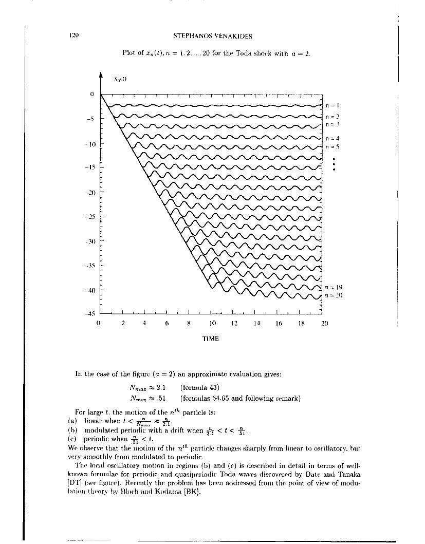
1210 STEPFIANOS VENAKIDES

Plot of x~, (t), it 1. 2,..20 for the Toda shock with a =2.

-5 2i

fl 4-10

-I5

-20

-25

-30)

-35

n=~ 19-40

n =20

0 2 4 6 8 10 12 14 16 18 20

TIME

In the case of the figure (a = 2) an approximate evaluation gives:

,V,,- 2. 1 (formula 43)

Nmin ýz .51 (formulas 64.65 and following remark)

For large t. the motion of the I-11 particle is:(a) linear when t N, n(b) modulated periodic with a drift when -- < t <n(c) periodic when .', < t.

We observe that the. motion of the 111 particle changes sharply from linear to oscillatory. butvery smoothly from modulated to periodic.

The local oscillatory motion in regions (b) and (c) is described in detail in terms of well-known formulae for periodic and quasiperiodic Toda waves dliscovered by Date arid Tanaka[DT] (see figure). Recently the. problem ha~s been addressed from the point of view of modu-lat ion thIe'orY by B~loch an(1 Kodarna [13K).

THE TODA SHOCK PROBLEM 121

2. Inverse Scattering and Lax Pairs

The Flaschka transformation

(4) a n-- , bn = (x,• - x.,)/2

22allows equations (1) to be written in Lax-pair [L] form:

dM(5) = BM- MB = -[M,B].

The tridiagonal matrices M and B are defined by:

(6) M(t) (" b, ba, bn , B(t) =( -6 "0 "bn

M is self-adjoint and B is antisymmetric in t 2 (Z). M(t) represents the state of the lattice attime t. Our initial data (2) are given in terms of the Flaschka variables by

1(7) an(0) = a sgn n, bn = -' n = 0, ±1, ±2,....

2To solve the initial value problem for (5) and (7) we employ the inverse scattering transfor-mation (IST) which recovers the matrix M from its scattering data, (SD). The latter consistof the spectrum and the asymptotic behavior of the eigenvectors of M as n -: ±Xc.

M(O) M(t)

IST IIST

evolution of SDSD(O) ,SD(t)

The scattering data are calculated in the next section by the spectral analysis of the matrixM(O). The evolution of the scattering data is easily obtained. One verifies by direct differen-tiation of (9) with respect to time that the one-parameter family of unitary operators definedby [L]

(8) U=BU, U(O) = I,

satisfies

(9) U-1 (t)M(t)U(t) = M(0)

when M and B satisfy (5). Thus. M(t) is unitarily equivalent to M(0) and the spectrum ofM(t) is independent of t. If V(t) is an eigenvector of M(t)

(10) 0(t) = U(t)p(0), d = Ut(t)g(0) = B(t)U(t).(O) =dt

In the limit n - ±oc, B(t) ... - 1/2 "0 1/2 . The evolution equation

for the asymptotic eigenvector, as n - ±+c becomes:

(11) d_••= "._1/2 "0 "1/2dt • . ..

The solution to the inverse scattering problem was discovered by Fadeev [F] who recoveredthe potential of the Schridinger operator directly from its scattering data. Previously, inlandmark work, Gelfand and Levitan fGL] had used the associated spectral function to recoverthe potential in a class satisfying much more general asymptotic conditions at infinity. Sincethen, the ideas of inverse scattering have been applied to many problems.

122 STEPHANOS VENAKII)ES

The theory of the scattering and inverse scattering transform for doubly infinite sElf-adjoitmatrices satisfying the asymptotic relations

(12) a,, -- a sgn a b. --- asn 1- ±X

with rapid convergence was derived by Oba [0]. As in the Fadeev study, the inverse p)roblem isreduced to solving a linear integral e(luation. the Marcenko equation. whose distribution kernelis computed in terms of the scattering data. In the context of the Schridinger operator. [)ys~o[M] has derived an explicit formula for the potential in terris of a F'redholhn deteriinait. Wederive a similar formula in the case of the Toda lattice. Our derivation, following Dyson.sreasoning, is more direct than the one employed in [VDO].

3. The Scattering Data (supercritical case a > 1)

The eigenvalue equation M(0)'V7 = AV, is equivalent to the set of scalar equations

(13) + aV, + ao n+. = -V',., n = 0, ±1, ±2, a,, = a sgn n.

Inserting V.,, = z" into all equations except those indexed by n = -1.0, 1. we find that AM(0)has formal eigenvectors:

(A+z' + B+z-' when n > 0(14) ¢ = A-z + B-z-_ when n < 0,

in which z± are related to the spectral variable A through the equation

1 1(15) - (z± + -- )-- (A -TZ a), jz+1 <_ I.2 Z

Of the five unknown constants A±, B± and 00 three are determined from the equations (13)indexed by n. = -1.0.1. One more constant is determined by the requirement that theeigenvector be bounded. We easily find that this can occur exactly when

(16) A E (T(M)= [-a - 1,-a+ 1] U {0} U [a - 1,a + 1]

The eigenvectors are real. They have multiplicity one and they satisfy the symmetry relation:

(17) •,(A) =

Explicitly for n > 0:

(18) V5. (A) ={(z)z" + S(z)z' whenA E [a - l.a + 1]

z c(z)z" whenA E [-a - 1.-a + 1] U {0}.

Where z = z+(A).


The map between the spectral variables z = z, and A is shown below.

A B 0 C I

A =-a-lICa

B=-a+ I D=a+ I

The upper spectral band CD = [a - 1, a + 1] is mapped onto the unit circle izi = 1: by (18)the eigenvectors oscillate when n > 0. The lower spectral band AB = [-a - 1. -a + 1] is

mapped onto the interval B'A' and the eigenvalue A = 0 is mapped onto point 0'; ill thiscase Izi < 1. so the eigenvectors decay as n -+-c. By (17), the eigenvector >,,,(A) decaysas n -- -oc whenever 0,(-A) decays as n +oc. 'O(A) oscillates as n -- -)c whenever7,(-A) oscillates as n - +x.

The normalizing constant c is arbitrary and determines S uniquely. We fix c by requiringthat IS(z)I = 1 on the continuous spectrum and letting the proper eigenvector at A = 0 haveunit i 2 norm. If our lattice were not starting with a pure shock but the initial condition (2)were satisfied only asymptotically as In -c oc then (18) would hold onfy asymptotically asn - +oc. This asymptotic behavior clearly persists when t > 0 with S and c dependent on t.The evolution of S and c is determined from (11):

(19&20) c(zt) = c(z,0)e½-)t, S(zt) = S(zO)e

We observe that c grows exponentially in t (-1 < z < 0) while S has unit modulus (IzI 1)for all t. The derivation and the evolution of the scattering data is done rigorously in [0].

4. The Solution to the Inverse Problem

The solution to the inverse problem is based on the beautiful observation of Gelfand and

Levitan [GLJ that the asymptotic eigenvectors O(A) defined in our case by

) ) S(z)z- + S(z)z' when A E [a-la +11

( =c(z)z' when A E {0} U [-a - 1,-a + 1]

are related to the normalized eigenvectors (,(A) by a Volterra transformation which is inde-pendent of A:

(22) 0i = Z QjsV,' Qjj independent of A.j=i

To convince ourselves of this we first note (nonrigorously) that relation (22) houls asymptot-ically as j -- +-)c in which case Oj - ,,j. We complete the argument by showing that if (22)

is true for all i > p then it is also true for i = p - 1. Indeed, solving the basic relation1 1

(23) -¢p-, + a~p + -op = A0P22

124 STEPHANOS VENAKIDES

for Op-1 we obtain:

Op-1 2A4 p, - 2a(P, - 0,,1=

(24) ZT2Qpj(4Aj) - 2aQpj , - Qp+,, qj]j=p

We now insert the relation:

(25) AXj = bj-'- 1 + aj3 O + bj1 1+i,

to obtain

(26) p- 2 2 Qpjbj-~j- + linear comb. of Oj s with j > p.j=p

This proves the statement and also yields

(27) Qp- ,p-- 2bp- Qpp.

There follows

(28) Q = I(2bp)= exp XP - = expX2 X

p=n p=n

The latter statement is true provided that 2b, tends to 1 sufficiently fast as p +Dc.In accordance with the spectral theorem, the normalized eigenvectors satisfy the relation

(29) f V,'m(A)n(A)dp(A) = b,,

The measure dp(A) is absolutely continuous with respect to Lebesgue measure on the contin-uous spectrum and is atomic at the eigenvalue A = 0. It can be determined exactly by Stone'sformula. This will not be needed for our calculation. We code the scattering data into thematrix

(30) Fp= p(A)Oj(A)dp(A).

Relation (29) combined with V '- 0, as i - +-c imply

(31) Fpt - bpi, when p.f -- x.

"•e insert (22) into (30) and use (29). For equations (32) only. we use the convention thatrepelated indices are summed over. The matrix Qpf is upper triangular. 'A,( have

(32) Fp, = J ¢,(A)O(A)dp(A) =

(summation convention) = Q, Qf.7•l, (A) u, (A)dp(A) =

= ,(A)hj(A)dj,(A)

= Qme~hi =Q,,)Qf.


Let F, denote the matrix Fpt truncated to have entries p. > n + 1. The upper triangular

matrix Q,, is defined in a similar way.We have

(33) F, = QQT, detF,,, {detQ,} 2 .

For the rapid convergence of initial data which we assume as n -±-+V. the matrix Q can beshown to equal the identity plus a trace class matrix, thus the determinants are well-defined.Recalling that Q,, is triangular we obtain

(34) detFn = { l QPp} 2

p=rn+

Combining (34) and (28) we obtain

(35) Xn = x. + irt F Idet F,,"

This solves the inverse scattering problem.We calculate the matrix F,.

a+ 1 2i_9

(36) Fpt = f (Sz-P + SzP)(Sz-e + Sz,)dp(A) + c2 zP+'dp(A)

Recalling that JSI2 = 1 we obtain

a+1 a

(37) Fpe= (zP-' + z'f-)dp(A) + (S 2 z-p- + S2 zP+t)dp(A)

,0+

+ La-1 c2 zP+tdp(A).

where the upper limit 0+ means that the atom at zero is included. The first integral equals6pe (Kronecker delta). Indeed, for fixed difference p - i take p and t to tend to +0c. The lasttwo integrals tend to zero. The statement follows directly from (31).

Ansatz I. We can neglect the second integral in (37).The integral in question is oscillatory and decays as t - +oc while the third integral grows

exponentially (cf. relation (19)). This does not constitute a rigorous argument since it is stillconceivable that small changes in the entries of the matrix F,, can produce a large change inthe (determinant of F,. Nevertheless. this step of our calculation is supported by the fact thatour solution is in full agreement with the results of numerical experiments.

It is important to note that the region of validity of our Ansatz ranges from a negativevalue of • to +,Y. For more negative values of , the solution obtained through the Ansatzis not spatially antisymmetric and thus obviously wrong. It is not surprising that the regionof validity of the Ansatz is not antisymmetric. The use of inverse scattering which favors oneof the two spatial directions breaks the antisymmetry of the original problem.

Since our initial data are antisymmetric we only need to calculate for ! > 0, thus the regionof validity of the Ansatz suffices for our purpose. In the case of nonantisymmetric initial datawe would have to obtain the solution by doing inverse scattering from the right for positiven's and from the left for negative n's. Using the Ansatz we write:

,0-4

(Fj = bpi + c 2(z. t)zP+edp(A).

Denoting the integral in (38) by Fp, we have

(39) det F, = det(1 + F,P) = det(hp, + Fp,)p.>,1+1

By our statement following (33) the matrix F,,. belongs to the trace class.

126 STEPHANOS VENAKII)ES

5. Calculation of the Determinant

We expand the determinant of (I + sFn) in powers of s and then set s I. W\e obtain

(39a) det(Fn) = 1 + Zd(n. k),k=1

where

d(n. k)= 1mk=n4-1 r 1 n+l

Inserting the value of FI using the multilinear dependence of the determinant on its coluhmsand interchanging summation and integration we obtain

(40) d(n.k) =1

I +rnz *.n zI + Z -a2

a- I. I I. zdp(,A,) ... dp(APIk)k! i a-- 1 mn•=n+l mj=nýl "" .

where ci = c(zj. t).By factoring z'I' from the ith row and multiplying it into the ith column we write the

determinant in the integrand as det(ziz1 ),fi where i, j = 1..... k. Using the nmultilineardependence of the determinant on its columns we can perform the summations.

((z zj ) n+I k 2n+2 I ~ ... kMultiple Sum =det\ ) = ( det 1-ziz j 1. k.

By exploiting the facts that (i) the determinant in (40) vanishes when z, = z, and (ii) tiledenominator of the expanded determinant has known form we obtain

(41) det 1 ) <

(I -l f-Lj=l ... k(1 - z'z )

Finally absorbing { 12 C2 (Z.,)j into tile measure dp(A) which becomes df(A) and utilizingthe symmetry of the integrand we have

(42) d(v. k) = ] exp 1 [nfnz j z -)t]

-+- l<: 1..<: fn<0+ ýA) . j)A

j=1 1=1I I ?Zz

6. Long-Time Behavior

We consider the limit t. - -..c while } N > 0 where N is held fixed. The double sum ill(42) has negative terms and has order O(k 2 ). The z 's can be chosen so that the single surmis positive aind has order O(kt) provided Nfnz2 + z - 7 is positive for some subinterval of the


lower spectral )and. This happens exactly when N is in the interval [0. Nxam ) where

(43) Ninax - V (/• +" 1)it) (,/a- + ,,7+ )"

In this icgion of N. tihe maxinimn of t Pi integrand will arise when the single and double sumisin (42) ha ', the same order of magnitude. in other words when k 0= (t). The exponent thenwill have order Q(t2).

The main contribution to the integral for d(n. k) will arise at the points which maximize theexponent. For a given k let there be a local maximum of the exponent at point (A I.... Ak).We recall that A1 is related to the z, of expression (42) by relation (15) with z, = z.. A, = A.The domain of the Ai's is the union 1-a-1.-a+ 1]U{0}. All the A,'s are distinct since A, = A)for i - j makes a term of the double sum in (42) equal to - D-. Thus, we recognize two ty pes ofmnaxinizing points, one in which all of the A,'s are in [-a - 1. -a + 1] and one in which k - 1 ofthe A,'s lie in the band [-a-I. -a+ 11 and the kth one equals zero. We l)ostulate one maximizerof each type. The postulate is confirmed by the subsequent analysis (section 7). We label thetwo maximizers (A' ..... A'.) and (A' ..... A 1 , 0) where the A"s and A"'s are in [-a - 1. -a +1. We denote their contributions to d(n. k) by Ak expmIlaxAE[_a-- i.-a+l Ek(A1 ...... Ak) andBk exp llmaxA,C--, 1 .- a+ Ek(A 1 . ... Ak_ .0) respectively. Here Ek is the expression for theexponent in (42) and Ak and Bk are coefficients which have the physical units of the productmeasurt. Thus

(44) (let F, Z{Ak exp max Ek(Ai... Ak)k HE-a--1.-a+11

+Bk+lexp max Ek+i(A.. Ak.0)}.E(a-l-~a.A i

Following Lax and Levermore [LL] we represent the points (A1 .... A k) by atomic measures

k(415) (A, . Ak) -.-- 6(A - Ai) dr'k.

t

Defining the functions:

(46) f(A) = 1l,,z2(A) + z(A) -t z (A)

L(A.p) Iin z(A) - z(p) wtr 1--z(A)z-p) when 1i $ A

(47) = 0 when p = A

we write, the exponent in (42) as

"f2 f /V LW d '(,T8) Ek = I. fd'. +/L(dk x

We (lescrJ)e our procedure for the maximization of the first term in (4.4). The maximizationof the, second term is done as a piert urbation of t he first term.

128 STEPHANOS VENAKI)ES

First we approximate the atomic inasure dt'ik by1 ani absolutely cont inioums Ieasure u.'(, A)dAsatisfying a

(1) positivity condition v > ()(2) mass constervation ((iant 1n) condition

(49) c- J,(A)dA = A= integer.

We obtain the quadratic fumctional

(50) /21(4) = -IdA f IA+ L(A. jL).(A)m ')dAd 1 }71'-fu- I 1a- 1 1a-

which approximiates Ek. Using the standard notat io for the inner product ill L[- -- 1. -a + I]and denoting by L the integrai operator with (list rihutioni kernel L(A. /) we write

t 2

(50a) E(4) = -- [(f. t:,) + (LV', U')].

It can be estimated that

(51) max Ek(AI ..... Ak) = max E(m, ) + klnk - )(k) when k = O(t).I - x.A ), E'- CA - 1,-- + l] tE.Ak

4k is tHIe set of measurable functions on [-a - 1. -a + 1] satisfying the positivity (condlitionamid thie (ataintum condition. The "'neasure coefficient" Ak ill (4-4) can also be estimat ed

(52) Ak = C-khtk+°(k)

We observe lhat the terms klh., in (51 ) and (52) cancel ill (53).

(53) Ak eXP max Ek(A .I A) =At,E'-a-1.-a+lj= extKp "max E(-ý,)+O(k

I~j {OE Ak (}

= exp[E(Vk) + O(k)].

whelre .k solwvs the nliaxiinization problem in the right hand side of (51).We JIOW turn tto the secondri term in the series (44). To the meastire (4,5) we adjioini all

additionial at o:i at A = 0. A pert urb)ation calculation gives

(51 k, i exI) Max ,Ek+I(AI. k.. ,) =

.4

k CxP max Ek(Al 1 .... Ak) + t[f(O) + 2L'k(O))] + rk}

w'here rk = ()(1),

"The quaillt itv f(0) + 2Lc4k(() is t he first variation of the fmn'ctijonal (f. v') + (Lc. 4') evaluatedat /,ro. i.e,. at the position of ilt extra attto i.

Iitvvrt Ing •53) and 15-1) into {-W) we obtain,

5,-, ,let F, -- I + Z ,,xp[E(.,,k) + ((kfl){ I + exp[t(f(0.) - 2Lb,-.(0)) + rtj}

Ak


where tk, constrained Y)y the positivity and qualit 111 conditions. maximizes the furictiotal

(50a). Formula (55) is rigorous as long as Ansatz I of section 4 is valid. We outline the-

procd(hure of maximization.

7. The Maximization Problem

\\'( insert

(56) , - , + •- + -- + .

1i 11 (i (50a' ) to obl)taill

E() -[(f. ,') + (Lt", + .--- (f + 2L-'. 0)

I -~

(57,, + (f + 2L'. 4-) + (L,. )t +

I WV dt(rmihte v, by max ':z;ng the leading order O(t2) term subject to thie positivity

c(ndit ion. "lw variational con(lit ion for the leading order probl)hm is

f(A) + 2L v.,(A) = 0 if C"(A) > 0

< 0 if C(A) = 0.

When Ct(A) = 0 thr, inequality L; not a priori strict, It is shown to be strict once the prolblemis solved. The solution is unique: L can be shown to be strictly negative definite.

2. We maximize tie(' Ott) order term (f + 2L'. t*,) (for the 1w " obtained from IlIhe leadilg()rde(r proleh~m) subject to (a) positivi! y: C(A) > 0 if C,,(A) = 0 (b) quantum (t onditio)n

JT .i t4"( A)dA + ( J,-" ti A)dA = '. Usin (.58) we easily see that the1 (t) term in (57)7

is maximized when

i 5,xa) i;-(A) =0 if L,*(A) = 0.

3. WCe maximize the O(1) term with respect to c, and v . Th(e argument of the previous

paragraph igives t-(A) 0 (I if C' (A) 0I which imnplies (f + 21 . -') 0. By looking at higher

orders we cart show v' - ... - 0. Contititig on the O(1) terin. we maximize (Lt'. 0

sun• ject t') to t he quantum condition oil thle support of C. (A). The variational conditiois are

Lt.(A) = - ei n A E sii) pp , (i : Lagrange mnultiiplier)

f 59) 4 '(A) = 0 when A E su1)1) t'

-(). + (it - A = 0 (tuantil ut colifditiont

(60) where {- I - when A E ,lpA C=where , . - " 1(A) )0 when A E 5s1l)1)V.

1lw(, solutions are paramet rizedr by k A ETh1 variati(oal equiatiorts (58) and (59) are reduced to Miemann- Iillbert prob)lhems through

Ie 1wobsrvat ion:

I (dz(A) -. d I 1(6il -z(A) - - L(A vp) =V(•11) 2 - I x

2rr (/A dA A- it

130 srEPHAN( )S VENAKIIDES

The sohltions to (58) and (59) are obtained inl terms of elliptic integrals.

WXe list the rs-ults and we refer to [VD}() for the proofs. When 0 < N < N ..... (N,,,,, < N,,nris defined in the paragraph following (65)).

(62) (-(A) - R0(A) A E [-a - 1 -a+ 1+

Ru (A)

where

(63)Ro(A)=[(A-+ aa+1)(A+a-1)(A-a+1)(A-a-1)]12 , Ro(A) >0 as A + +x

(64)PO (A) = A2 + NA + Co,

and co < 0 is uniquely determined. independently of N, by the relation

(65) a P(A) dA = 0.

_f+ alI (-,A)

This solution is valid only when N ranges from zero (we only consider N > 0) to the valueN ... at which Pn(-a + 1) = 0. As N increases from the value Ntu,. one of the roots ofPFl enters the interval [-a - 1. -a + 1] and the positivity of i," is violated. The support of

" for N > N. recedes to [-a - 1. -(N)]. where -a - I < < -a + 1. We have for

yNzy < N < Nm,,.

y;"(A) = -i P(A) when A E [-a -R (A)

(66) = 0 otherwise

where

(67) R(A) = [(A + a + 1)(A - -')(A - a + 1)(.\ - a - 1)]1/2. R(A) > 0 when A - +v

(68) P(A) = A2 + (N + -a2

The real constants -y and c are determined from:

(69) P(-y) = 0. R(A) 0.

As N increases further, 'Y decreases. At the value N equal

(70) N.,V + l, .-)(va + vI+ )"

i attains the value -a - 1. in which case V,'(A) - 0. When N > N,,,,,.r we have in (39)

det F,, - 1. The value t r N,,m, is the speed of the progressing front.


The first variation of the leading order functional is

(71) J(A) f(A) + 2L)* (A) = 2 R(A,)dA' when - a - 1 < A < -

=2 2 P(A) dA' when -'< A <a- 1,A R(A')

If A E[-a- l'](=-a+ I when 0< N < N"Itl).

-i' dA'(7-2) k(A) =jk Lk = Ek (A' - constant.

-R(A) R(A')

The constants Ek, where k is an integer. are determined front the qu,.ntum condition

(73) iEk (dA at - k. (a defineid by (60)).7r -L-1 R(A)

8. The Local Structure of the Waveform

The appearance of the elliptic curve R(A) in the previous section is significant. Explicitperiodic and qua(siperiodic solutions of the Toda lattice have been derived in terms of thetheta function corresponding to an elliptic curve by Date and Tanaka [DT].

For fixed N, we can identify the solution described by (55) with the solutions obtained

by Date and Tanaka. Thus. (55) is a modulated (varying with N) quasiperiodic solution ofthe Toda lattice. The equations (69) which give the dependence of Y on N can be properlythoughit of as modulation equations. When 0 < N < N'_,_ there is no modulation: y =

-a + 1. We carry out the identification in the latter region of N and we omit the identificationin the modulating region Nmn < N < N~naZ. We describe the behavior at the boundary n = 0.

We use the results stated in the previous section to calculate explicitly when 0 < N < Nmzn

\r obtain:

(74) - (f, ) =N 2 17?(4a) - 4aN + constant.7r"

1 -ir f-l+i_ A2 +c

(75) 1 = -2N + v. X = f- RA -cdA = pure real.2 7r J. ioR0 (A)

a-i dAR(X)

(76) L2"ýk(0) 2 irir(2 - 't + k). r -- pure imaginary.=.- dI - +_ i ,R

(77) f(0) - 2Li<°(0) = -J-" j -na.

(78) (LV7;k, ',k) = irr&(at - ) 2 < 0.

We insert these in (55). We use the following Ansatz which is natural but which we have

not, succeeded in proving.Ansatz II: the ((k) term in (55) has an asymptotic expansion in k which is ralid at Ieast

up to constants (k to the zero power). Similarly rk - r where r is a constant.

132 STEPHANOS VENAKIl)ES

Given the Ansatz, the C)(k) term ill ('55) would only affect our calculation up to a phalseshift and up to a constant term added to xy. We neglect the O(k) term and obtain

(79) det F,,(t) ,-exp[- ln(4a) - 2ant]}

x + exp[-ju + r + (k + - wt)7uT] I + _ -it) 2I.k=1 2 2

We can replace the lower summation limit k - I with k = - xc. since the main contribui 1il:to the series comes from k's which satisfy k , wt - = ("J - )t = at. where a > 0 (see(60)). We define the function

(80) P(rj) = '

This is reduced readily to the standard theta function.

(81) O(z) = , e27rtkz wi+-k2

k=-xc

through the relationO =e 12 0(7).

In terms of the p-function we write after a straightforward calculation

(82) det F,,(t) -{exp[~ It2n(4a) - 2antj

x -P Wt) + mn +r(2 - Wt +2)

How can we derive the boundary condition xo(t) = 0 from this formula? We have

(83) xo(t) = -2at + In dtF tdet F0(t)

"We insert the expression (82) for detF,(t) using the notation p = p(-Wt) and P1/2 =

p(-Lt - ½) and recalling that p(r7 + 1) = p(i/). After a very short calculation we obtain- +r

(84) xo(t) = In4a + In P112 + PC r

p + e +rPl/2

Taking the remark following (78) into account we write

(84a) xo(t) = const. + Ill P12 + PeJ +rP1/2 + pe 4

The condition xo(t) = independent of t. is satisfied if and only if7riT

(85) j 717+2r=0, (recall j=lna)2

which determines r. It would be very satisfying to verify this by direct calculation, withoutrelying on the symmetry of the problem. At present, this delicate calculation is unfortunatelybeyond our reach.

To arrive at a final formula for x,,(t) we insert the value of r which satisfies (85) into (82).We insert the latter into (35). We determine the unknown constant in the local mean valueof x,,(t) so that xo(t) = 0. We obtain after a short calculation

(86) x, (t) = -n n4a + I Ina + In A(n .t)2 A A(), t)


where

(87) A(n,. t) = - (t -Wt+ 1)1 < m,,.

By the antisvynmetry of our problenm thi formula is valid not only in the region 0 < < L' ra,

but also in tihe region -N..,, < L < 0. When Inj >> 1. either the first (vi > 0) or the second

term (n < 0) dominate in (87). The solution in this case is identified with a space-periodic,time-periodic Toda wave. As expected by the antisyrnmetry of the problem the p functionsin the two terms are out of phase by a half-period. When Injl is small (i.e. near the boundaryparticle n = 0) both terms in (87) must be taken into account.

The formula for x,(t) can then be identified with the formula obtained by Date and Tanakaif we take the latter with spectrum

[-a - 1. -a + 1] U [-6,. ] U [a - 1. a + 1]

and let 6 - 0, in which case we obtain our degenerate structure

[-a - 1, -a + 1] U {0} U [a - 1,a + 1].

Alternatively we can obtain our solution from a periodic solution with spectrum [-a - 1. -a +1] U (a - 1, a + 1 which is Darboux transformed and an eigenvalue is inserted at the origin.

REFERENCES

[BKI A.M, Block and Y. Kodamna, lsperxve Regularization of the Whitham Equatto for the Toda Lattice, preprint.[Dj F. Dyson, Old and new approaches to the inverse scatter9ng problem. Essays in honor of Valentine Bargmann

ed. E. H. Leib, B. Simon and A. S. Wightman Princeton Univ. Press. Princeton, NJ.. Studies in Math.Phys. (1976).

JDTJ E. Date and S. Tanaka, Periodic Mult olitons of the Korteweg~de Vries Equaton and Toda Lattwc. Progr.Theoret. Phys. Suppl. 59 (1976), 107-125.

[F] L. D. Faddeyev, The inverse problem in the quantum theory of scattering, Usp. Mat. Nauk. 14 (1959); englishtranslation, J. Math. Phys. 4 (1963). 72-,104.

[GLI I.M. Gel'fand and B.M. Levitan, On the determination of a differential equaton from its spectralfunctiomr Izv.Akad. Nauk. SSSR. Ser. Mat. 15 (1951); english translation, AMS Translations 2 (1955), 253-304.

[HFMI B. L. Holian. H. Flaschka, D. W. McLaughlin, Shock Waves in the Toda Lattice: ArWatys., Physical Rev.A 24 # 5 (Nov. 1981). 2595-2623.

[HS) B.L. Holian and G.K. Straub. Molecular dynamics of shock uwves in one dimensional chains. Phys. Rev. B.18 (1978), 1593.

ILI P. D. Lax, Integrals of Nonlinear Equations of Evolution and Solitary Waves, Comm. Pure Appl. Math. 21(1968). 467-490.

[O0 R. Oba, Doubly Infinite Toda Lattce with Anti&,nmetric Asymptotics. Ph.D. Thesis. Courant Inst. 1988.1 VDOI S. Venakides, P. Delft and R. Oba. The Toda Shock Problem, Comm. Pure Appl. Math (to appeax).

Department of MathematicsDuke University

Durham, NC 27706

sl a - dtic · 2011-05-14 · integration, topology, and geometry in 14 lectures on nielsen fixed...

Documents