slab on grade on shrink swell soil: a new...
TRANSCRIPT

SLAB ON GRADE ON SHRINK SWELL SOIL: A NEW METHOD
The Cross‐USA Lecture
Professor Jean‐Louis BRIAUD
Distinguished ProfessorTexas A&M University

CONTENT1. Shrink Swell Soils: a Background
2. Development of the method
3. The design charts
4. Superposition of loads
5. Verification
6. Case history
7. Example by hand
8. TAMU‐SLAB: Excel spread sheet


Water content – volume change model

WATER NORMAL STRESS
(SUCTION)
(pF )
TENSION COMPRESSION
0 uw (kPa)
(PORE PRESSURE)
UNSATURATED SATURATED

Foundation solutionsfor shrink swell soils

EXISITNG METHODS
1. BRAB (Building Research Advisory Board, 1968)
2. WRI (Wire Reinforcing Institute, 1981)
3. AS2870 (Australian Standard, 1996)
4. PTI (Post Tensioning Institute, 2012)
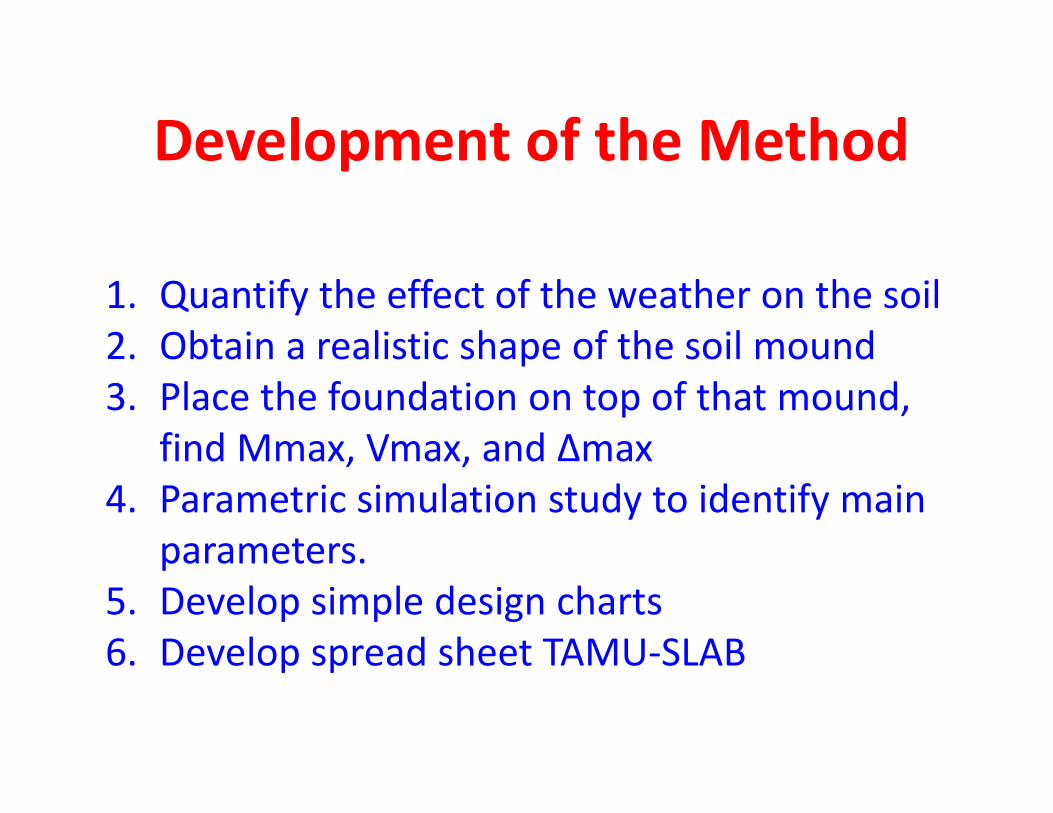
Development of the Method
1. Quantify the effect of the weather on the soil 2. Obtain a realistic shape of the soil mound3. Place the foundation on top of that mound,
find Mmax, Vmax, and Δmax4. Parametric simulation study to identify main
parameters.5. Develop simple design charts6. Develop spread sheet TAMU‐SLAB


Weather Effect on the Soil
College
Station
San
AntonioAustin Dallas Houston Denver
log (uf max / uf min) 0.788 1.392 0.866 1.295 1.283 1.374
log (ue max / ue min) 0.394 0.696 0.433 0.648 0.642 0.687

Water content vs Time (2 years)

Realistic Shape of Mound
2 211 12 12
2 1221 21122
2 1 exp 2 cosh2 2 1
cosh22
n
nfield field
h edgen
field
H H xn nHx f H ULH nnnH
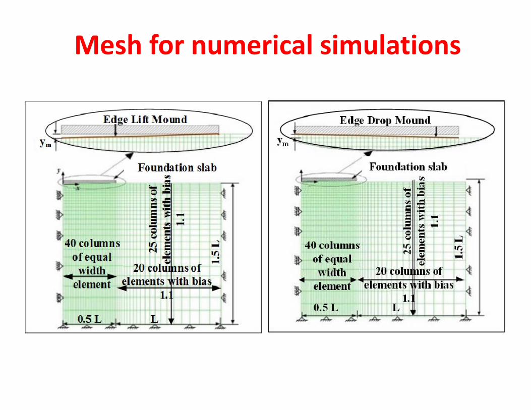
Mesh for numerical simulations

Example results of Abaqussimulation

Most Important Input Parameters
1. Shrink‐swell index ISS2. Depth of the active zone H
3. Change of soil surface water tension (suction)
ue max /ue min
4. Slab stiffness represented by the equivalent
flat slab thickness d

Soil Weather Index
max
min
1 log2
e
eSW SS
uu
I I H
SW eI H w
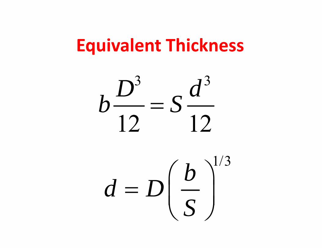
Equivalent Thickness
3 3
12 12D db S
1/3bd DS

EDGE DROPUNIFORM LOAD
0.0
1.0
2.0
3.0
4.0
5.0
6.0
7.0
8.0
0.00 0.50 1.00EQ
UIV
AL
EN
T L
EN
GT
H L
eqv
(m)
SOIL WEATHER INDEX Isw = H.∆we
p = 10kpa
0.63
0.51
0.38
0.25
0.13
d (m)

EDGE DROPLINE LOAD (EDGE)
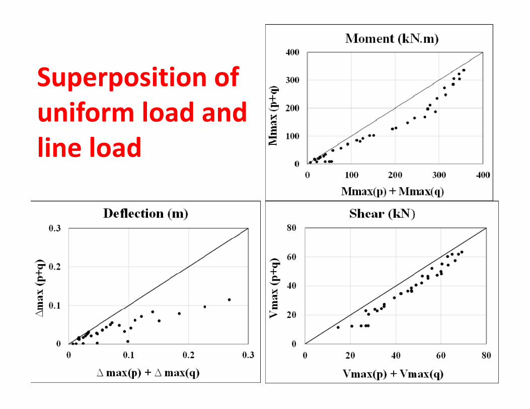
Superposition of uniform load and line load

Predictions vs mean prediction
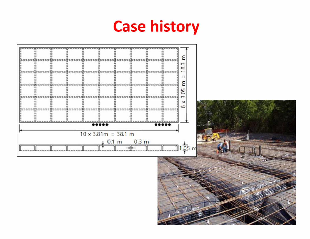
Case history

Soil movement vs depth (5 meters)

Soil movement vs time (2 years)

INPUT: Depth of active zone H = 3.0 m,Water content Δwf = 20%,Slab 20 m x 20 m,Beams S = 3.0 m, D = 1.2m, b = 0.3 m,Load p = 10 kPa, q = 10 kN/m.
CRITERION: L/Δ > 360
CALCULATION: Water content at edge of the slabΔwe = 0.5Δwf = 0.5 x 0.2 = 0.1,Soil weather index Isw = H x Δwe = 3 x 0.1 = 0.3m,Slab stiffness EI = EbD3/12 = 2 x 107 x 0.3 x 1.23/12 = 8.64 x 10⁵kNm2,Equivalent depth d = D (b/S)1/3 = 1.2(0.3/3)1/3 = 0.56m
CHARTS: Uniform pressure: Leqv = 5.11m, Fv = 0.70, and FΔ = 2.21Line load: Leqv = 7.07m, Fv = 1, FΔ = 2.12
DESIGN EXAMPLE

MOMENT, SHEAR, DEFLECTION CALCULATIONS
Uniform pressure Spacing of 3 m: P = 10 x 3 = 30kN/mMmax = PLeq
2/2 = 30 x 5.112/2 = 392kNmVmax = Fv P Leq = 0.70 x 30 x 5.11 = 107.31kNΔmax = PLeq
4/FΔEI = 30 x 5.114/2.21x 8.64x105 = 1.07 x 10⁻²m.
Line load Spacing of 3 m: Q = 3 x10 = 30kNMmax = Q Leqv = 30 x 7.07 = 212kN.mVmax = Fv Q = 1 x 30 kN = 30kNΔmax = Q Leqv
3/FΔEI = 30 X 7.073/2.12 X 8.64 X 105 = 5.80 X 10⁻³m.
Combined load Mmax(p) + Mmax(q) = 392 + 212 = 604kNmVmax (p) + Vmax(q) = 107.3 + 30 kN = 137.3kNΔmax (p) +Δmax (q) = 1.07 x 10⁻²+ 5.80 X 10-3 = 1.65 x 10⁻²m.
CHECK DISTORTION Leqv(ave) /Δmax = (5.11+7.07)/2 / 1.65 x 10 -2 = 369 > 360.
DESIGN EXAMPLE

TAMU‐SLAB
• Excel SPREAD SHEET
• AUTOMATES THE DESIGN PROCESS
• INPUT SOIL, WEATHER, SLAB, LOAD
• CONTAINS ALL DESIGN CHARTS
• CALCULATES MOMENT, SHEAR, DEFLECTION
• CHECKS DISTORTION CRITERION
• TRIAL AND ERROR APPROACH