slides enbal
TRANSCRIPT

8/20/2019 Slides Enbal
http://slidepdf.com/reader/full/slides-enbal 1/182
The Energy Balance for Chemical Reactors
Copyright c 2011 by Nob Hill Publishing, LLC
• To specify the rates of reactions in a nonisothermal reactor, we require a
model to determine the temperature of the reactor, i.e. for the reaction
A + B k1 k−1
C
r = k1( T ) cAcB − k−1( T ) cC
• The temperature is determined by the energy balance for the reactor.
• We derive the energy balance by considering an arbitrary reactor volume ele-
ment, shown in Figure 1
1

8/20/2019 Slides Enbal
http://slidepdf.com/reader/full/slides-enbal 2/182
General Energy Balance
m1
E 1cj1
m0
E 0
cj0
V
Q W
Figure 1: Reactor volume element.
2

8/20/2019 Slides Enbal
http://slidepdf.com/reader/full/slides-enbal 3/182
The statement of conservation of energy for this system takes the form,
rate of energy
accumulation
=
rate of energy
entering system
by inflow
−
rate of energy
leaving system
by outflow
+
rate of heat
added to system
+
rate of work
done on system
(1)
In terms of the defined variables, we can write Equation 1 as,
dE
dt = m0E 0 − m1E 1 + Q + W (2)
in which the hat indicates an energy per unit mass.
3

8/20/2019 Slides Enbal
http://slidepdf.com/reader/full/slides-enbal 4/182
Work Term
It is convenient to split the work term into three parts: W f , the work done
by the flow streams while moving material into and out of the reactor, W s, the
shaft work being done by stirrers, compressors, etc., and W b, the work done
when moving the system boundary.
W total work
= W f
flow streams
+ W s shaft work
+ W b boundary work
(3)
4

8/20/2019 Slides Enbal
http://slidepdf.com/reader/full/slides-enbal 5/182
Work done by the flow streams
W f = v0A0P 0 − v1A1P 1 = Q0P 0 − Q1P 1
5

8/20/2019 Slides Enbal
http://slidepdf.com/reader/full/slides-enbal 6/182
P 0
v0
v1
P 1
A0
A1V
Figure 2: Flow streams entering and leaving the volume element.
We also can express the volumetric flowrate as a mass flowrate divided by
6

8/20/2019 Slides Enbal
http://slidepdf.com/reader/full/slides-enbal 7/182
the density, Q = m/ρ
W f = m0P 0
ρ0− m1
P 1
ρ1
The overall rate of work can then be expressed as
W = W f + W s + W b = m0P 0
ρ0− m1
P 1
ρ1+ W s + W b (4)
7

8/20/2019 Slides Enbal
http://slidepdf.com/reader/full/slides-enbal 8/182
Energy Terms
The total energy may be regarded as composed of many forms. Obvious
contributions to the total energy arise from the internal, kinetic and potential
energies.1
E = U + K + Φ + · · ·
For our purposes in this chapter, we consider only these forms of energy. Re-
calling the definition of enthalpy, H = U + P V , or expressed on a per-unit mass
basis, H = U + P /ρ, allows us to rewrite Equation 2 as
d
dt (U + K + Φ) = m
0 H + K + Φ0− m
1 H + K + Φ1+ Q + W
s+ W
b (5)
1In some cases one might need to consider also electrical and magnetic energies. For example, we might
consider the motion of charged ionic species between the plates in a battery cell.
8

8/20/2019 Slides Enbal
http://slidepdf.com/reader/full/slides-enbal 9/182
The Batch Reactor
Since the batch reactor has no flow streams Equation 5 reduces to
d
dt(U + K + Φ) = Q + W s + W b (6)
In chemical reactors, we normally assume the internal energy is the dominant
contribution and neglect the kinetic and potential energies. Normally we neglect
the work done by the stirrer, unless the mixture is highly viscous and the stirring
operation draws significant power [3]. Neglecting kinetic and potential energies
and shaft work yieldsdU
dt + P
dV Rdt
= Q (7)
in which W b = −P dV R/dt.
9

8/20/2019 Slides Enbal
http://slidepdf.com/reader/full/slides-enbal 10/182
Batch reactor in terms of enthalpy
It is convenient to use enthalpy rather than internal energy in the subsequent
development. Taking the differential of the definition of enthalpy gives for V =
V RdH = dU + P dV R + V RdP
Forming the time derivatives and substitution into Equation 7 gives
dH
dt − V R
dP
dt = Q (8)
10

8/20/2019 Slides Enbal
http://slidepdf.com/reader/full/slides-enbal 11/182
Effect of changing T , P , nj
For single-phase systems , we consider the enthalpy as a function of temper-
ature, pressure and number of moles, and express its differential as
dH = ∂H
∂T P ,nj
dT + ∂H
∂P T ,nj
dP + j ∂H
∂njT,P,nk
dnj (9)
The first partial derivative is the definition of the heat capacity, C P .
C P = V RρC P
The second partial derivative can be expressed as∂H
∂P
T ,nj
= V − T
∂V
∂T
P ,nj
= V (1 − αT )
11

8/20/2019 Slides Enbal
http://slidepdf.com/reader/full/slides-enbal 12/182
in which α = (1/V)(∂V/∂T)P ,nj is the coefficient of expansion of the mixture.
The final partial derivatives are the partial molar enthalpies, H j
∂H
∂nj
T,P,nk
= H j
so Equation 9 can be written compactly as
dH = V RρC P dT + (1 − αT)V RdP +
j
H jdnj (10)
12

8/20/2019 Slides Enbal
http://slidepdf.com/reader/full/slides-enbal 13/182
Meanwhile, back in the batch reactor
Forming the time derivatives from this expression and substituting into Equa-
tion 8 gives
V RρC P dT
dt − αT V R
dP
dt +
j
H jdnj
dt = Q (11)
We note that the material balance for the batch reactor is
dnj
dt = RjV R =
nr i=1
νijr iV R, j = 1, . . . , ns (12)
which upon substitution into Equation 11 yields
V RρC P dT
dt − αT V R
dP
dt = −
i
∆H Rir iV R + Q (13)
13

8/20/2019 Slides Enbal
http://slidepdf.com/reader/full/slides-enbal 14/182
in which ∆H Ri is the heat of reaction
∆H Ri =
jνijH j (14)
14

8/20/2019 Slides Enbal
http://slidepdf.com/reader/full/slides-enbal 15/182
A plethora of special cases – incompressible
We now consider several special cases. If the reactor operates at constant
pressure (dP/dt = 0) or the fluid is incompressible (α = 0), then Equation 13
reduces to
Incompressible-fluid or constant-pressure reactor.
V RρC P dT
dt = −
i
∆H Rir iV R + Q (15)
15

8/20/2019 Slides Enbal
http://slidepdf.com/reader/full/slides-enbal 16/182
A plethora of special cases – constant volume
Change from T , P , nj to T , V , nj by considering P to be a function of T , V ( V =
V R), nj
dP =
∂P
∂T
V ,nj
dT +
∂P
∂V
T ,nj
dV +
j
∂P
∂nj
T,V,nk
dnj
For reactor operation at constant volume, dV = 0, and forming time derivativesand substituting into Equation 11 gives
V RρC P − αT V R
∂P
∂T
V ,nj
dT
dt +
j
H j − αT V R
∂ P
∂nj
T,V,nk
dnj
dt = Q
We note that the first term in brackets is C V = V RρC V [4, p. 43]
V RρC V = V RρC P − αT V R
∂P
∂T
V ,nj
16

8/20/2019 Slides Enbal
http://slidepdf.com/reader/full/slides-enbal 17/182
Substitution of C V and the material balance yields the energy balance for the
constant-volume batch reactor
Constant-volume reactor.
V RρC V dT
dt
= −i ∆H Ri − αT V R j
νij ∂P
∂njT,V,nk r iV R + Q (16)
17

8/20/2019 Slides Enbal
http://slidepdf.com/reader/full/slides-enbal 18/182
Constant volume — ideal gas
If we consider an ideal gas, it is straightforward to calculate αT = 1 and
(∂P/∂nj)T,V,nk = RT /V . Substitution into the constant-volume energy balance
gives
Constant-volume reactor, ideal gas.
V RρC V dT
dt = −
i
(∆H Ri − RT νi) r iV R + Q (17)
where νi = jνij.
18

8/20/2019 Slides Enbal
http://slidepdf.com/reader/full/slides-enbal 19/182
Constant-pressure versus constant-volume reactors
Example 6.1: Constant-pressure versus constant-volume reactors
Consider the following two well-mixed, adiabatic, gas-phase batch reactors for
the elementary and irreversible decomposition of A to B,
A k → 2B (18)
Reactor 1: The reactor volume is held constant (reactor pressure therefore
changes).
Reactor 2: The reactor pressure is held constant (reactor volume therefore
changes).
19

8/20/2019 Slides Enbal
http://slidepdf.com/reader/full/slides-enbal 20/182
Both reactors are charged with pure A at 1.0 atm and k has the usual Arrhenius
activation energy dependence on temperature,
k(T) = k0 exp(−E/T)
The heat of reaction, ∆H R, and heat capacity of the mixture, C P , may be assumed
constant over the composition and temperature range expected.
Write the material and energy balances for these two reactors. Which reactor
converts the reactant more quickly?
20

8/20/2019 Slides Enbal
http://slidepdf.com/reader/full/slides-enbal 21/182
Solution — Material balance
The material balance isd(cAV R)
dt = RAV R
Substituting in the reaction-rate expression, r = k(T)cA, and using the number
of moles of A, nA = cAV R yields
dnA
dt = −k(T)nA (19)
Notice the temperature dependence of k(T) prevents us from solving this
differential equation immediately.
We must solve it simultaneously with the energy balance, which provides the
information for how the temperature changes.
21

8/20/2019 Slides Enbal
http://slidepdf.com/reader/full/slides-enbal 22/182
Energy balance, constant volume
The energy balances for the two reactors are not the same. We consider first
the constant-volume reactor. For the A → 2B stoichiometry, we substitute the
rate expression and ν = 1 into Equation 17 to obtain
C V dT dt
= − (∆H R − RT ) knA
in which C V = V RρC V is the total constant-volume heat capacity.
22

8/20/2019 Slides Enbal
http://slidepdf.com/reader/full/slides-enbal 23/182
Energy balance, constant pressure
The energy balance for the constant-pressure case follows from Equation 15
C P dT
dt = −∆H RknA
in which C P = V RρC P is the total constant-pressure heat capacity. For an ideal
gas, we know from thermodynamics that the two total heat capacities are simply
related,
C V = C P − nR (20)
23

8/20/2019 Slides Enbal
http://slidepdf.com/reader/full/slides-enbal 24/182
Express all moles in terms of nA
Comparing the production rates of A and B produces
2nA + nB = 2nA0 + nB0
Because there is no B in the reactor initially, subtracting nA from both sides
yields for the total number of moles
n = nA + nB = 2nA0 − nA
24

8/20/2019 Slides Enbal
http://slidepdf.com/reader/full/slides-enbal 25/182
The two energy balances
Substitution of the above and Equation 20 into the constant-volume case
yieldsdT
dt = −
(∆H R − RT ) knA
C P − (2nA0 − nA)R constant volume (21)
and the temperature differential equation for the constant-pressure case is
dT
dt = −
∆H RknA
C P constant pressure (22)
25

8/20/2019 Slides Enbal
http://slidepdf.com/reader/full/slides-enbal 26/182
So who’s faster?
We see by comparing Equations 21 and 22 that the numerator in the constant-
volume case is larger because ∆H R is negative and the positive RT is subtracted.
We also see the denominator is smaller because C P is positive and the positive
nR is subtracted.
Therefore the time derivative of the temperature is larger for the constant-
volume case. The reaction proceeds more quickly in the constant-volume case.
The constant-pressure reactor is expending work to increase the reactor size,
and this work results in a lower temperature and slower reaction rate compared
to the constant-volume case.
26

8/20/2019 Slides Enbal
http://slidepdf.com/reader/full/slides-enbal 27/182
Liquid-phase batch reactor
Example 6.2: Liquid-phase batch reactor
The exothermic elementary liquid-phase reaction
A + B k → C, r = kcAcB
is carried out in a batch reactor with a cooling coil to keep the reactor isothermal
at 27◦C. The reactor is initially charged with equal concentrations of A and B and
no C, cA0 = cB0 = 2.0 mol/L, cC 0 = 0.
1. How long does it take to reach 95% conversion?
27

8/20/2019 Slides Enbal
http://slidepdf.com/reader/full/slides-enbal 28/182
2. What is the total amount of heat (kcal) that must be removed by the cooling
coil when this conversion is reached?
3. What is the maximum rate at which heat must be removed by the cooling coil
(kcal/min) and at what time does this maximum occur?
4. What is the adiabatic temperature rise for this reactor and what is its signifi-
cance?
Additional data:
Rate constant, k = 0.01725 L/mol·min, at 27◦C
Heat of reaction, ∆H R = −10 kcal/mol A, at 27◦C
Partial molar heat capacities, C P A = C P B = 20 cal/mol·K, C P C =
40 cal/mol K
Reactor volume, V R = 1200 L
28

8/20/2019 Slides Enbal
http://slidepdf.com/reader/full/slides-enbal 29/182
Solution
1. Assuming constant density, the material balance for component A is
dcA
dt = −kcAcB
The stoichiometry of the reaction, and the material balance for B gives
cA − cB = cA0 − cB0 = 0
or cA = cB. Substitution into the material balance for species A gives
dcA
dt = −kc2
A
29

8/20/2019 Slides Enbal
http://slidepdf.com/reader/full/slides-enbal 30/182
Separation of variables and integration gives
t =
1
k 1
cA −
1
cA0
Substituting cA = 0.05cA0 and the values for k and cA0 gives
t = 551 min
2. We assume the incompressible-fluid energy balance is accurate for this liquid-
phase reactor. If the heat removal is manipulated to maintain constant reactor
temperature, the time derivative in Equation 15 vanishes leaving
Q = ∆H Rr V R (23)
Substituting dcA/dt = −r and multiplying through by dt gives
dQ = −∆H RV RdcA
30

8/20/2019 Slides Enbal
http://slidepdf.com/reader/full/slides-enbal 31/182
Integrating both sides gives
Q = −∆H RV R(cA − cA0) = −2.3 × 10⁴ kcal
3. Substituting r = kc2A into Equation 23 yields
Q = ∆H Rkc2AV R
The right-hand side is a maximum in absolute value (note it is a negative
quantity) when cA is a maximum, which occurs for cA = cA0, giving
Qmax = ∆H Rkc2A0V R = −828 kcal/min
4. The adiabatic temperature rise is calculated from the energy balance without
the heat-transfer term
V RρC P dT
dt = −∆H Rr V R
31

8/20/2019 Slides Enbal
http://slidepdf.com/reader/full/slides-enbal 32/182
Substituting the material balance dnA/dt = −r V R gives
V RρˆC P dT =
∆H RdnA (24)
Because we are given the partial molar heat capacities
C P j = ∂H j
∂T P ,nk
it is convenient to evaluate the total heat capacity as
V RρC P =
ns
j=1
C P jnj
For a batch reactor, the number of moles can be related to the reaction extent
by nj = nj0 + νjε, so we can express the right-hand side of the previous
32
8/20/2019 Slides Enbal
http://slidepdf.com/reader/full/slides-enbal 33/182
equation asns
j=1
C P jnj = j
C P jnj0 + ε∆C P
in which ∆C P =
j νjC P j. If we assume the partial molar heat capacities are
independent of temperature and composition we have ∆C P = 0 and
V RρC P =
nsj=1
C P jnj0
Integrating Equation 24 with constant heat capacity gives
∆T = ∆H
Rj C P jnj0
∆nA
The maximum temperature rise corresponds to complete conversion of the
33

8/20/2019 Slides Enbal
http://slidepdf.com/reader/full/slides-enbal 34/182
reactants and can be computed from the given data
∆T max = −10 × 103 cal/mol
2(2 mol/L)(20 cal/mol K)(0 − 2 mol/L)
∆T max = 250 K
The adiabatic temperature rise indicates the potential danger of a coolant
system failure. In this case the reactants contain enough internal energy toraise the reactor temperature by 250 K.
34

8/20/2019 Slides Enbal
http://slidepdf.com/reader/full/slides-enbal 35/182
The CSTR — Dynamic Operation
d
dt (U + K + Φ) = m0
H + K + Φ
0
− m1
H + K + Φ
1
+ Q + W s + W b (25)
We assume that the internal energy is the dominant contribution to the total
energy and take the entire reactor contents as the volume element.
We denote the feed stream with flowrate Qf , density ρf , enthalpy H f , and
component j concentration cjf .
The outflow stream is flowing out of a well-mixed reactor and its intensive
properties are therefore assumed the same as the reactor contents.
35

8/20/2019 Slides Enbal
http://slidepdf.com/reader/full/slides-enbal 36/182
Its flowrate is denoted Q. Writing Equation 5 for this reactor gives,
dU
dt = Qf ρf H f − Qρ H + Q + W s + W b (26)
36

8/20/2019 Slides Enbal
http://slidepdf.com/reader/full/slides-enbal 37/182
The CSTR
If we neglect the shaft work
dU
dt + P
dV R
dt = Qf ρf H f − Qρ H + Q
or if we use the enthalpy rather than internal energy (H = U + P V )
dH
dt − V R
dP
dt = Qf ρf H f − Qρ H + Q (27)
37

8/20/2019 Slides Enbal
http://slidepdf.com/reader/full/slides-enbal 38/182
The Enthalpy change
For a single-phase system we consider the change in H due to changes in
T , P , nj
dH = V RρC P dT + (1 − αT)V RdP +
j
H jdnj
Substitution into Equation 27 gives
V RρC P dT
dt − αT V R
dP
dt +
j
H jdnj
dt = Qf ρf
H f − Qρ H + Q (28)
The material balance for the CSTR is
dnj
dt = Qf cjf − Qcj +
i
νijr iV R (29)
38

8/20/2019 Slides Enbal
http://slidepdf.com/reader/full/slides-enbal 39/182
Substitution into Equation 28 and rearrangement yields
V RρC P
dT
dt − αT V RdP
dt = −
i∆H Rir iV R +
j
cjf Qf (H jf − H j) + Q (30)
39

8/20/2019 Slides Enbal
http://slidepdf.com/reader/full/slides-enbal 40/182
Special cases
Again, a variety of important special cases may be considered. These are
listed in Table 9 in the chapter summary. A common case is the liquid-phase
reaction, which usually is well approximated by the incompressible-fluid equa-
tion,
V RρC P dT dt
= −
i
∆H Rir iV R +
j
cjf Qf (H jf − H j) + Q (31)
In the next section we consider further simplifying assumptions that require less
thermodynamic data and yield useful approximations.
40

8/20/2019 Slides Enbal
http://slidepdf.com/reader/full/slides-enbal 41/182
CSTR — Summary of energy balances
Neglect kinetic and potential energiesdU
dt = Qf ρf
H f − Qρ H + Q + W s + W b
Neglect shaft workdU
dt + P
dV Rdt
= Qf ρf H f − Qρ H + Q
dH
dt − V
R
dP
dt = Q
f ρ
f
H f
− Qρ H + Q
Single phase
V RρC P dT
dt − αT V R
dP
dt +
j
H j
dnj
dt = Qf ρf
H f − Qρ H + Q
V RρC P dT
dt − αT V R
dP
dt = −
i
∆H Rir iV R +j
cjf Qf (H jf − H j ) + Q
a. Incompressible-fluid or constant-pressure reactor
V RρC P dT
dt = −
i
∆H Rir iV R +j
cjf Qf (H jf − H j) + Q
41

8/20/2019 Slides Enbal
http://slidepdf.com/reader/full/slides-enbal 42/182
b. Constant-volume reactor
V RρC V dT
dt = −
i ∆H Ri − αT V R j
νijP njr iV R +
jcjf Qf (H jf − H j) + αT V R j
P nj(cjf Qf − cj Q) + Q
b.1 Constant-volume reactor, ideal gas
V RρC V dT
dt = −
i
∆H Ri − RT νi
r iV R +
j
cjf Qf (H jf − H j) + RT j
(cjf Qf − cj Q) + Q
c. Steady state, constant C P , P = P f
−i
∆H Rir iV R + Qf ρf C P (T f − T ) + Q = 0
Table 1: Energy balances for the CSTR.
42

8/20/2019 Slides Enbal
http://slidepdf.com/reader/full/slides-enbal 43/182
Steady-State Operation
If the CSTR is at steady state, the time derivatives in Equations 29 and 30
can be set to zero yielding,
Qf cjf − Qcj + i
νijr iV R = 0 (32)
−
i
∆H Rir iV R +
j
cjf Qf (H jf − H j) + Q = 0 (33)
Equations 32 and 33 provide ns + 1 algebraic equations that can be solved si-
multaneously to obtain the steady-state concentrations and temperature in the
CSTR. Note that the heats of reaction ∆H Ri are evaluated at the reactor temper-
ature and composition.
43

8/20/2019 Slides Enbal
http://slidepdf.com/reader/full/slides-enbal 44/182
Liquid phase, Steady-State Operation
If the heat capacity of the liquid phase does not change significantly with
composition or temperature, possibly because of the presence of a large excess
of a nonreacting solvent, and we neglect the pressure effect on enthalpy, which
is normally small for a liquid, we obtain
H jf − H j = C P j(T f − T )
Substitution into Equation 33 gives
−
i
r i∆H RiV R + Qf ρf C P (T f − T ) + Q = 0 (34)
44

8/20/2019 Slides Enbal
http://slidepdf.com/reader/full/slides-enbal 45/182
Temperature control in a CSTR
An aqueous solution of species A undergoes the following elementary reac-
tion in a 2000 L CSTR
Ak1
k−1
R ∆HR = −18 kcal/mol
Q1
Q2
2525◦C
45

8/20/2019 Slides Enbal
http://slidepdf.com/reader/full/slides-enbal 46/182
The feed concentration, C Af , is 4 mol/L and feed flowrate, Qf , is 250 L/min.
The reaction-rate constants have been determined experimentally
k1 = 3 × 10⁷e−5838/T min−1
K 1 = 1.9 × 10⁻¹¹e9059/T
1. At what temperature must the reactor be operated to achieve 80% conversion?
2. What are the heat duties of the two heat exchangers if the feed enters at 25◦C
and the product is to be withdrawn at this temperature? The heat capacity of
feed and product streams can be approximated by the heat capacity of water,
C P = 1 cal/g K.
46

8/20/2019 Slides Enbal
http://slidepdf.com/reader/full/slides-enbal 47/182
Solution
1. The steady-state material balances for components A and R in a constant-
density CSTR are
Q(cAf − cA) − r V R = 0
Q(cRf − cR) + r V R = 0
Adding these equations and noting cRf = 0 gives
cR = cAf − cA
Substituting this result into the rate expression gives
r = k1(cA − 1
K 1(cAf − cA))
47

8/20/2019 Slides Enbal
http://slidepdf.com/reader/full/slides-enbal 48/182
Substitution into the material balance for A gives
Q(cAf − cA) − k1(cA −
1
K 1 (cAf − cA))V R = 0 (35)
If we set cA = 0.2cAf to achieve 80% conversion, we have one equation and
one unknown, T , because k1 and K 1 are given functions of temperature. Solv-
ing this equation numerically gives
T = 334 K
48

8/20/2019 Slides Enbal
http://slidepdf.com/reader/full/slides-enbal 49/182
Watch out
Because the reaction is reversible, we do not know if 80% conversion is achiev-
able for any temperature when we attempt to solve Equation 35.
It may be valuable to first make a plot of the conversion as a function of
reactor temperature. If we solve Equation 35 for cA, we have
cA = Q/V R + k1/K 1
Q/V R + k1(1 + 1/K 1)cAf
or for xA = 1 − cA/cAf
xA = k1
Q/V R + k1(1 + 1/K 1) =
k1τ
1 + k1τ(1 + 1/K 1)
49

8/20/2019 Slides Enbal
http://slidepdf.com/reader/full/slides-enbal 50/182
xA versus T
0
0.2
0.4
0.6
0.8
1
240 260 280 300 320 340 360 380 400
T (K)
xA
We see that the conversion 80% is just reachable at 334 K, and that for any
conversion lower than this value, there are two solutions.
50

8/20/2019 Slides Enbal
http://slidepdf.com/reader/full/slides-enbal 51/182
Heat removal rate
2. A simple calculation for the heat-removal rate required to bring the reactor
outflow stream from 334 K to 298 K gives
Q2 = Qf ρC P ∆T
= (250 L/min)(1000 g/L)(1 cal/g K)(298 − 334 K)
= −9 × 10³ kcal/min
Applying Equation 34 to this reactor gives
Q1 = k1(cA −
1
K 1 (cAf − cA))∆H RV R − Qf ρC P (T f − T )
= −5.33 × 10³ kcal/min
51

8/20/2019 Slides Enbal
http://slidepdf.com/reader/full/slides-enbal 52/182
Steady-State Multiplicity
• The coupling of the material and energy balances for the CSTR can give rise
to some surprisingly complex and interesting behavior.
• Even the steady-state solution of the material and energy balances holds some
surprises.
• In this section we explore the fact that the steady state of the CSTR is not
necessarily unique.
• As many as three steady-state solutions to the material and energy balances
may exist for even the simplest kinetic mechanisms.
• This phenomenon is known as steady-state multiplicity.
52

8/20/2019 Slides Enbal
http://slidepdf.com/reader/full/slides-enbal 53/182
An Example
We introduce this topic with a simple example [6]. Consider an adiabatic,
constant-volume CSTR with the following elementary reaction taking place in
the liquid phase
A k → B
We wish to compute the steady-state reactor conversion and temperature. The
data and parameters are listed in Table 2.
53

8/20/2019 Slides Enbal
http://slidepdf.com/reader/full/slides-enbal 54/182
Parameters
Parameter Value Units
T f 298 K
T m 298 K
C P 4.0 kJ/kg K
cAf 2.0 kmol/m3
km 0.001 min−1
E 8.0 × 10³ K
ρ 103 kg/m3
∆H R −3.0 × 10⁵ kJ/kmol
U o 0
Table 2: Parameter values for multiple steady states.
54

8/20/2019 Slides Enbal
http://slidepdf.com/reader/full/slides-enbal 55/182
Material Balance
The material balance for component A is
d(cAV R)
dt = Qf cAf − QcA + RAV R
The production rate is given by
RA = −k(T)cA
For the steady-state reactor with constant-density, liquid-phase streams, the ma-
terial balance simplifies to
0 = cAf − (1 + kτ)cA (36)
55
8/20/2019 Slides Enbal
http://slidepdf.com/reader/full/slides-enbal 56/182
Rate constant depends on temperature
Equation 36 is one nonlinear algebraic equation in two unknowns: cA and T .
The temperature appears in the rate-constant function,
k(T) = kme−E(1/T −1/T m)
Now we write the energy balance. We assume the heat capacity of the mixture
is constant and independent of composition and temperature.
56

8/20/2019 Slides Enbal
http://slidepdf.com/reader/full/slides-enbal 57/182
Energy balance
b. Constant-volume reactor
V RρC V dT
dt = −
i
∆H Ri − αT V R
j
νijP nj
r iV R +
j
cjf Qf (H jf − H j) + αT V Rj
P nj(cjf Qf − cj Q) + Q
b.1 Constant-volume reactor, ideal gas
V RρC V dT
dt = −
i
∆H Ri − RT νi
r iV R +
j
cjf Qf (H jf − H j) + RT j
(cjf Qf − cj Q) + Q
c. Steady state, constant C P , P = P f
−i
∆H Ri
r i
V R
+ Qf
ρf
C P
(T f
− T ) + Q = 0
Table 3: Energy balances for the CSTR.
57

8/20/2019 Slides Enbal
http://slidepdf.com/reader/full/slides-enbal 58/182
Energy balance
We assume the heat capacity of the mixture is constant and independent of
composition and temperature.
With these assumptions, the steady-state energy balance reduces to
0 = −kcA∆H RV R + Qf ρf C P (T f − T ) + U oA(T a − T )
Dividing through by V R and noting U o = 0 for the adiabatic reactor gives
0 = −kcA∆
H R +
C P s
τ (T f − T ) (37)
in which C P s = ρf C P , a heat capacity per volume.
58

8/20/2019 Slides Enbal
http://slidepdf.com/reader/full/slides-enbal 59/182
Two algebraic equations, two unknowns
0 = cAf − (1 + k(T)τ)cA
0 = −k(T)cA∆H R +
C P s
τ (T f − T )
The solution of these two equations for cA and T provide the steady-state
CSTR solution.
The parameters appearing in the problem are: cAf , T f , τ, C P s, km, T m, E ,∆H R. We wish to study this solution as a function of one of these parameters,
τ, the reactor residence time.
59

8/20/2019 Slides Enbal
http://slidepdf.com/reader/full/slides-enbal 60/182
Let’s compute
• Set ∆H R = 0 to model the isothermal case. Find cA(τ) and T (τ) as you vary
τ, 0 ≤ τ ≤ 1000 min.
• We will need the following trick later. Switch the roles of cA and τ and find
τ(cA) and T (cA) versus cA for 0 ≤ cA ≤ cAf .
• It doesn’t matter which is the parameter and which is the unknown, you can
still plot cA(τ) and T (τ). Check that both approaches give the same plot.
• For the isothermal reactor, we already have shown that
cA = cAf
1 + kτ, x =
kτ
1 + kτ
60

8/20/2019 Slides Enbal
http://slidepdf.com/reader/full/slides-enbal 61/182
Exothermic (and endothermic) cases
• Set ∆H R = −3 × 10⁵ kJ/kmol and solve again. What has happened?
• Fill in a few more ∆H R values and compare to Figures 3–4.
• Set ∆H R = +5 × 10⁴ kJ/kmol and try an endothermic case.
61

8/20/2019 Slides Enbal
http://slidepdf.com/reader/full/slides-enbal 62/182
Summary of the results
0
0.1
0.2
0.3
0.4
0.5
0.6
0.7
0.8
0.9
1
1 10 100 1000 10000 100000
τ (min)
x
−30−20−10
−50
+5
Figure 3: Steady-state conversion versus residence time for different values of
the heat of reaction (∆H R × 10−4 kJ/kmol).
62
8/20/2019 Slides Enbal
http://slidepdf.com/reader/full/slides-enbal 63/182
260
280
300
320
340
360
380
400
420
440
460
1 10 100 1000 10000 100000
τ (min)
T (K)
−30−20−10
−5
0+5
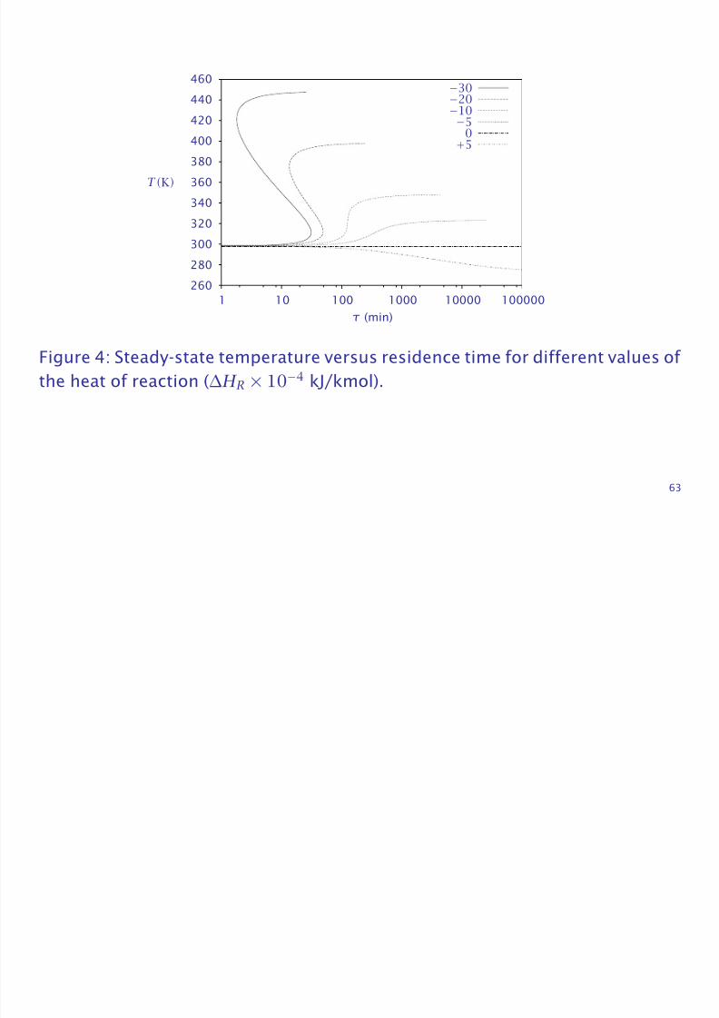
Figure 4: Steady-state temperature versus residence time for different values of
the heat of reaction (∆H R × 10−4
kJ/kmol).
63

8/20/2019 Slides Enbal
http://slidepdf.com/reader/full/slides-enbal 64/182
Steady-state multiplicity, ignition, extinction
• Note that if the heat of reaction is more exothermic than −10 kJ/kmol, there
is a range of residence times in which there is not one but several steady-state
solutions, three solutions in this case.
• The reactor is said to exhibit steady-state multiplicity for these values of
residence time.
• The points at which the steady-state curves turn are known as ignition and
extinction points.
64

8/20/2019 Slides Enbal
http://slidepdf.com/reader/full/slides-enbal 65/182
0
0.1
0.2
0.3
0.4
0.5
0.6
0.7
0.8
0.9
1
0 5 10 15 20 25 30 35 40 45
τ (min)
ignition point
extinction point
x
•
•
Figure 5: Steady-state conversion versus residence time for
∆H R = −3 × 10⁵ kJ/kmol; ignition and extinction points.
65

8/20/2019 Slides Enbal
http://slidepdf.com/reader/full/slides-enbal 66/182
280
300
320
340
360
380
400
420
440
460
0 5 10 15 20 25 30 35 40 45
τ (min)
ignition point
extinction point
T (K)
•
•
Figure 6: Steady-state temperature versus residence time for
∆H R = −3 × 10⁵
kJ/kmol; ignition and extinction points.
66
8/20/2019 Slides Enbal
http://slidepdf.com/reader/full/slides-enbal 67/182
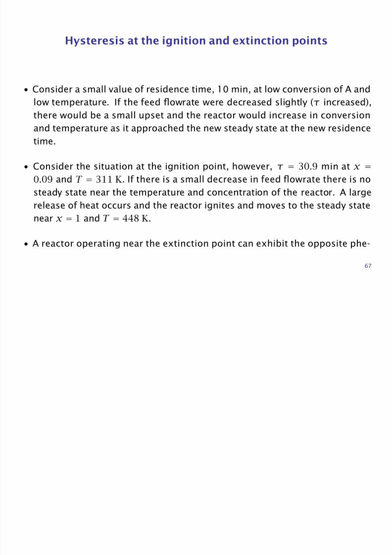
Hysteresis at the ignition and extinction points
• Consider a small value of residence time, 10 min, at low conversion of A and
low temperature. If the feed flowrate were decreased slightly (τ increased),
there would be a small upset and the reactor would increase in conversion
and temperature as it approached the new steady state at the new residence
time.
• Consider the situation at the ignition point, however, τ = 30.9 min at x =
0.09 and T = 311 K. If there is a small decrease in feed flowrate there is no
steady state near the temperature and concentration of the reactor. A large
release of heat occurs and the reactor ignites and moves to the steady state
near x = 1 and T = 448 K.
• A reactor operating near the extinction point can exhibit the opposite phe-
67

8/20/2019 Slides Enbal
http://slidepdf.com/reader/full/slides-enbal 68/182
nomenon. A small increase in feed flowrate causes the residence time to
decrease enough so that no steady-state solution exists near the current
temperature and concentration. A rapid drop in temperature and increase
in concentration of A occurs as the reactor approaches the new steady state.
68

8/20/2019 Slides Enbal
http://slidepdf.com/reader/full/slides-enbal 69/182
Stability of the Steady State
We next discuss why some steady states are stable and others are unstable.
This discussion comes in two parts. First we present a plausibility argument and
develop some physical intuition by constructing and examining van Heerdendiagrams [7].
The text also presents a rigorous mathematical argument, which has wide
applicability in analyzing the stability of any system described by differential
equations.
Dynamic Model
69

8/20/2019 Slides Enbal
http://slidepdf.com/reader/full/slides-enbal 70/182
We examine the stability numerically by solving the dynamic model.
dcA
dt =
cAf − cA
τ − kcA (38)
dT
dt =
U oA
V RC P s(T a − T ) +
T f − T
τ −
∆H R
C P skcA (39)
70

8/20/2019 Slides Enbal
http://slidepdf.com/reader/full/slides-enbal 71/182
Steady-state temperature versus residence time
280
300
320
340
360
380
400
420
440
460
0 5 10 15 20 25 30 35 40
τ (min)
T (K)
•
•
•
• •
•
•
C
G
B
D
F
A
E
Figure 7: Steady-state temperature versus residence time for
∆H R = −3 × 10⁵ kJ/kmol.
71

8/20/2019 Slides Enbal
http://slidepdf.com/reader/full/slides-enbal 72/182
Heat generate and heat removal
If we substitute the the mass balance for cA into the energy balance, we
obtain one equation for one unknown, T ,
0 = − k
1 + kτcAf ∆H R
Qg
+C P s
τ (T f − T )
Qr
(40)
We call the first term the heat-generation rate, Qg. We call the second term
the heat-removal rate, Qr
,
Qg = − k(T)
1 + k(T)τcAf ∆H R, Qr =
C P s
τ (T − T f )
72

8/20/2019 Slides Enbal
http://slidepdf.com/reader/full/slides-enbal 73/182
in which we emphasize the temperature dependence of the rate constant,
k(T) = kme−E(1/T −1/T m)
73

8/20/2019 Slides Enbal
http://slidepdf.com/reader/full/slides-enbal 74/182
Graphical solution
Obviously we have a steady-state solution when these two quantities are
equal.
Consider plotting these two functions as T varies.
The heat-removal rate is simply a straight line with slope C P s/τ.
The heat-generation rate is a nonlinear function that is asymptotically con-
stant at low temperatures (k(T) much less than one) and high temperatures
(k(T) much greater than one).
These two functions are plotted next for τ = 1.79 min.
74

8/20/2019 Slides Enbal
http://slidepdf.com/reader/full/slides-enbal 75/182
Van Heerden diagram
−1 × 10⁵
0
1 × 10⁵
2 × 10⁵
3 × 10⁵
4 × 10⁵
5 × 10⁵
250 300 350 400 450 500
T (K)
•
•
A
E (extinction)
h e a t ( k J / m
3
·
m i n )
removalgeneration
Figure 8: Rates of heat generation and removal for τ = 1.79 min.
75

8/20/2019 Slides Enbal
http://slidepdf.com/reader/full/slides-enbal 76/182
Changing the residence time
Notice the two intersections of the heat-generation and heat-removal func-
tions corresponding to steady states A and E.
If we decrease the residence time slightly, the slope of the heat-removal line
increases and the intersection corresponding to point A shifts slightly.
Because the two curves are just tangent at point E, however, the solution at
point E disappears, another indicator that point E is an extinction point.
76

8/20/2019 Slides Enbal
http://slidepdf.com/reader/full/slides-enbal 77/182
Changing the residence time
The other view of changing the residence time.
280
300
320
340
360
380
400
420
440
460
0 5 10 15 20 25 30 35 40
τ (min)
T (K)
•
•
•
• •
•
•
C
G
B
D
F
A
E
77

8/20/2019 Slides Enbal
http://slidepdf.com/reader/full/slides-enbal 78/182
Stability — small residence time
If we were to increase the reactor temperature slightly, we would be to the
right of point A in Figure 8.
To the right of A we notice that the heat-removal rate is larger than the heat-
generation rate. That causes the reactor to cool, which moves the temperature
back to the left.
In other words, the system responds by resisting our applied perturbation.
Similarly, consider a decrease to the reactor temperature. To the left of
point A, the heat-generation rate is larger than the heat-removal rate causing
the reactor to heat up and move back to the right.
Point A is a stable steady state because small perturbations are rejected by
the system.
78

8/20/2019 Slides Enbal
http://slidepdf.com/reader/full/slides-enbal 79/182
Intermediate residence time
Consider next the points on the middle branch. Figure 9 displays the heat-
generation and heat-removal rates for points B, D and F, τ = 15 min.
280
300
320
340
360
380
400
420
440
460
0 5 10 15 20 25 30 35 40
τ (min)
T (K)
•
•
•
• •
•
•
C
G
B
D
F
A
E
79

8/20/2019 Slides Enbal
http://slidepdf.com/reader/full/slides-enbal 80/182
Intermediate residence time
−1 × 10⁴
0
1 × 10⁴
2 × 10⁴
3 × 10⁴
4 × 10⁴
5 × 10⁴
6 × 10⁴
250 300 350 400 450 500
T (K)
•
•
•
B
D (unstable)
F
h e a t ( k J / m
3
·
m i n )
removalgeneration
Figure 9: Rates of heat generation and removal for τ = 15 min.
80
8/20/2019 Slides Enbal
http://slidepdf.com/reader/full/slides-enbal 81/182
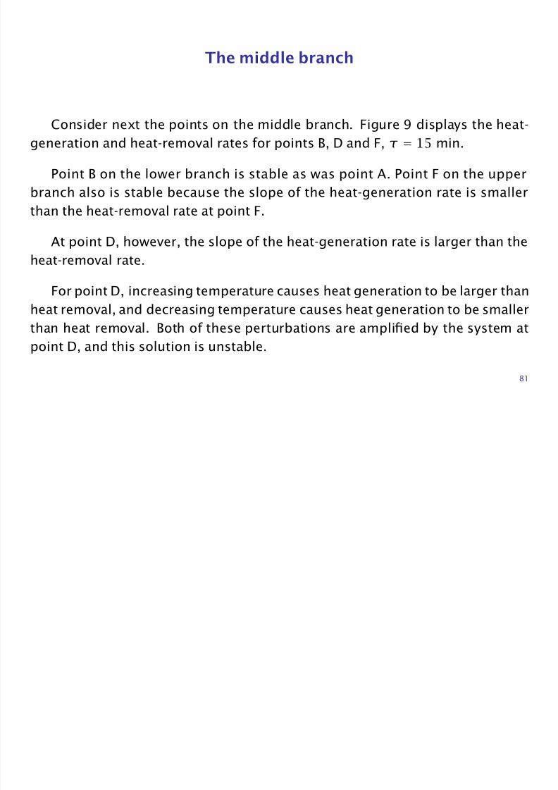
The middle branch
Consider next the points on the middle branch. Figure 9 displays the heat-
generation and heat-removal rates for points B, D and F, τ = 15 min.
Point B on the lower branch is stable as was point A. Point F on the upper
branch also is stable because the slope of the heat-generation rate is smaller
than the heat-removal rate at point F.
At point D, however, the slope of the heat-generation rate is larger than the
heat-removal rate.
For point D, increasing temperature causes heat generation to be larger than
heat removal, and decreasing temperature causes heat generation to be smaller
than heat removal. Both of these perturbations are amplified by the system at
point D, and this solution is unstable.
81

8/20/2019 Slides Enbal
http://slidepdf.com/reader/full/slides-enbal 82/182
All points on the middle branch are similar to point D.
82

8/20/2019 Slides Enbal
http://slidepdf.com/reader/full/slides-enbal 83/182
Large residence time
280
300
320
340360
380
400
420
440
460
0 5 10 15 20 25 30 35 40
τ (min)
T (K)
•
•
•
• •
•
•
C
G
B
D
F
A
E
83

8/20/2019 Slides Enbal
http://slidepdf.com/reader/full/slides-enbal 84/182
Large residence time
Next observe the heat-generation and heat-removal rates for τ = 30.9 min.
−5 × 10³
0
5 × 10³
1 × 10⁴
2 × 10⁴
2 × 10⁴
2 × 10⁴
3 × 10⁴
250 300 350 400 450 500
T (K)
C (ignition)
G
•
•
h e a t ( k J / m
3 · m
i n )
removal
generation
84

8/20/2019 Slides Enbal
http://slidepdf.com/reader/full/slides-enbal 85/182
Large residence time
Notice that point G on the upper branch is stable and point C, the ignition
point, is similar to extinction point E, perturbations in one direction are rejected,
but in the other direction they are amplified.
85

8/20/2019 Slides Enbal
http://slidepdf.com/reader/full/slides-enbal 86/182
Reactor Stability — Rigorous Argument
I will not cover this section in lecture. Please read the text.
86

8/20/2019 Slides Enbal
http://slidepdf.com/reader/full/slides-enbal 87/182
A simple mechanical analogy
You may find it helpful to draw an analogy between the chemical reactor with
multiple steady states and simple mechanical systems that exhibit the same
behavior.
Consider a marble on a track in a gravitational field as depicted in Figure 10.
87

8/20/2019 Slides Enbal
http://slidepdf.com/reader/full/slides-enbal 88/182
A simple mechanical analogy
88

8/20/2019 Slides Enbal
http://slidepdf.com/reader/full/slides-enbal 89/182
g
A
Figure 10: Marble on a
track in a gravitational
field; point A is the
unique, stable steady
state.89

8/20/2019 Slides Enbal
http://slidepdf.com/reader/full/slides-enbal 90/182
Single steady state
Based on our physical experience with such systems we conclude immedi-
ately that the system has a single steady state, position A, which is asymptoti-
cally stable.
If we expressed Newton’s laws of motion for this system, and linearized the
model at point A, we would expect to see eigenvalues with negative real part
and nonzero imaginary part because the system exhibits a decaying oscillation
back to the steady-state position after a perturbation.
The oscillation decays because of the friction between the marble and the
track.
90

8/20/2019 Slides Enbal
http://slidepdf.com/reader/full/slides-enbal 91/182
Multiple steady states
Now consider the track depicted in Figure 12.
91

8/20/2019 Slides Enbal
http://slidepdf.com/reader/full/slides-enbal 92/182
A simple mechanical analogy
92

8/20/2019 Slides Enbal
http://slidepdf.com/reader/full/slides-enbal 93/182
g
A
Figure 11: Marble on a
track in a gravitational
field; point A is the
unique, stable steady
state.
A C
g
B
Figure 12: Marble on a
track with three steady
states; points A and C
are stable, and point B
is unstable.93

8/20/2019 Slides Enbal
http://slidepdf.com/reader/full/slides-enbal 94/182
Multiple steady states
Here we have three steady states, the three positions where the tangent curve
to the track has zero slope. This situation is analogous to the chemical reactor
with multiple steady states.
The steady states A and C are obviously stable and B is unstable. Perturba-
tions from point B to the right are attracted to steady-state C and perturbations
to the left are attracted to steady-state A.
The significant difference between the reactor and marble systems is that
the marble decays to steady state in an oscillatory fashion, and the reactor, with
its zero imaginary eigenvalues, returns to the steady state without overshoot oroscillation.
94

8/20/2019 Slides Enbal
http://slidepdf.com/reader/full/slides-enbal 95/182
Ignition and extinction
Now consider the track depicted in Figure 15.
95

8/20/2019 Slides Enbal
http://slidepdf.com/reader/full/slides-enbal 96/182
A simple mechanical analogy
96

8/20/2019 Slides Enbal
http://slidepdf.com/reader/full/slides-enbal 97/182
g
A
Figure 13: Marble on a
track in a gravitational
field; point A is the
unique, stable steady
state.
A C
g
B
Figure 14: Marble on a
track with three steady
states; points A and C
are stable, and point B
is unstable.
g
CA
Figure 15: Marble ona track with an ignition
point (A) and a stable
steady state (C).
97
d

8/20/2019 Slides Enbal
http://slidepdf.com/reader/full/slides-enbal 98/182
Ignition and extinction
We have flattened the track between points A and B in Figure 12 so there is
just a single point of zero slope, now marked point A. Point A now corresponds
to a reactor ignition point as shown in Figures 5 and 6. Small perturbations
push the marble over to the only remaining steady state, point C, which remains
stable.
98
S l i S i d O ill i i i C l

8/20/2019 Slides Enbal
http://slidepdf.com/reader/full/slides-enbal 99/182
Some real surprises — Sustained Oscillations, Limit Cycles
The dynamic behavior of the CSTR can be more complicated than multiple
steady states with ignition, extinction and hysteresis.
In fact, at a given operating condition, all steady states may be unstable and
the reactor may exhibit sustained oscillations or limit cycles. Consider the same
simple kinetic scheme as in the previous section,
A k → B
but with the following parameter values.
99

8/20/2019 Slides Enbal
http://slidepdf.com/reader/full/slides-enbal 100/182
Param. Value Units
T f 298 KT m 298 K
C P 4.0 kJ/kg K
cAf 2.0 kmol/m3
km(T m) 0.004 min−1
E 1.5 × 10
4
Kρ 103 kg/m3
∆H R −2.2 × 10⁵ kJ/kmol
U oA/V R 340 kJ/(m3 min K)
Table 4: Parameter values for limit cycles.
Note: the last line of this table is missing in the first printing!
Notice that the activation energy in Table 4 is significantly larger than in
100
T bl 2

8/20/2019 Slides Enbal
http://slidepdf.com/reader/full/slides-enbal 101/182
Table 2.
101
E t i t d t d t t b h i

8/20/2019 Slides Enbal
http://slidepdf.com/reader/full/slides-enbal 102/182
Even more twisted steady-state behavior
If we compute the solutions to the steady-state mass and energy balances
with these new values of parameters, we obtain the results displayed in the next
Figures.
102

8/20/2019 Slides Enbal
http://slidepdf.com/reader/full/slides-enbal 103/182
0
0.1
0.2
0.3
0.4
0.5
0.6
0.7
0.8
0.9
1
0 20 40 60 80 100
τ (min)
x
Figure 16: Steady-state conversion versus residence time.
103

8/20/2019 Slides Enbal
http://slidepdf.com/reader/full/slides-enbal 104/182
280
300
320
340
360
380
400
420
0 20 40 60 80 100
τ (min)
T (K)
Figure 17: Steady-state temperature versus residence time.
If we replot these results using a log scaling to stretch out the x axis, we
obtain the results in Figures 18 and 19.
104

8/20/2019 Slides Enbal
http://slidepdf.com/reader/full/slides-enbal 105/182
0
0.2
0.4
0.6
0.8
1
0.001 0.01 0.1 1 10 100 1000
τ (min)
•
•
x
A
B
•••
•
C D
E
F
Figure 18: Steady-state conversion versus residence time — log scale.
105

8/20/2019 Slides Enbal
http://slidepdf.com/reader/full/slides-enbal 106/182
280
300
320
340
360
380
400
420
0.001 0.01 0.1 1 10 100 1000
τ (min)
•
•
T (K)
A
B
••
•
•
C D
E
F
Figure 19: Steady-state temperature versus residence time — log scale.
Notice the steady-state solution curve has become a bit deformed and the
simple s-shaped multiplicities in Figures 5 and 6 have taken on a mushroom
shape with the new parameters.
106

8/20/2019 Slides Enbal
http://slidepdf.com/reader/full/slides-enbal 107/182
We have labeled points A–F on the steady-state curves. Table 5 summarizes
the locations of these points in terms of the residence times, the steady-state
conversions and temperatures, and the eigenvalue of the Jacobian with largest
real part.
Point τ(min) x T (K) Re(λ)(min−1) Im(λ)(min−1)
A 11.1 0.125 305 0 0B 0.008 0.893 396 0 0
C 19.2 0.970 339 −0.218 0
D 20.7 0.962 336 −0.373 0
E 29.3 0.905 327 0 0.159
F 71.2 0.519 306 0 0.0330
Table 5: Steady state and eigenvalue with largest real part at selected points in
Figures 18 and 19.
107

8/20/2019 Slides Enbal
http://slidepdf.com/reader/full/slides-enbal 108/182
Now we take a walk along the steady-state solution curve and examine the
dynamic behavior of the system.
What can simulations can show us. A residence time of τ = 35 min is between
points E and F as shown in Table 5. Solving the dynamic mass and energy
balances with this value of residence time produces
108

8/20/2019 Slides Enbal
http://slidepdf.com/reader/full/slides-enbal 109/182
0
0.5
1
0 100 200 300 400 500 600280
300
320
340
360
380
400
x T (K)
time (min)
x(t)
T(t)
Figure 20: Conversion and temperature vs. time for τ = 35 min.
109
Is this possible?

8/20/2019 Slides Enbal
http://slidepdf.com/reader/full/slides-enbal 110/182
Is this possible?
We see that the solution does not approach the steady state but oscillates
continuously. These oscillations are sustained; they do not damp out at large
times. Notice also that the amplitude of the oscillation is large, more than 80 K
in temperature and 50% in conversion.
We can obtain another nice view of this result if we plot the conversion versus
the temperature rather than both of them versus time. This kind of plot is known
as a phase plot or phase portrait
110

8/20/2019 Slides Enbal
http://slidepdf.com/reader/full/slides-enbal 111/182
0
0.1
0.2
0.3
0.4
0.5
0.6
0.7
0.8
0.9
1
290 300 310 320 330 340 350 360 370 380 390 400
T (K)
x
Figure 21: Phase portrait of conversion versus temperature for feed initial con-
dition; τ = 35 min.
111

8/20/2019 Slides Enbal
http://slidepdf.com/reader/full/slides-enbal 112/182
Time increases as we walk along the phase plot; the reactor ignites, then
slowly decays, ignites again, and eventually winds onto the steady limit cycle
shown in the figure. The next figure explores the effect of initial conditions.
112

8/20/2019 Slides Enbal
http://slidepdf.com/reader/full/slides-enbal 113/182
0
0.1
0.2
0.3
0.4
0.5
0.6
0.7
0.8
0.9
1
290 300 310 320 330 340 350 360 370 380 390 400
T (K)
◦
x
Figure 22: Phase portrait of conversion versus temperature for several initial
conditions; τ = 35 min.
113

8/20/2019 Slides Enbal
http://slidepdf.com/reader/full/slides-enbal 114/182
The trajectory starting with the feed temperature and concentration is shown
again.
The trajectory starting in the upper left of the figure has the feed temperature
and zero A concentration as its initial condition.
Several other initial conditions inside the limit cycle are shown also, including
starting the reactor at the unstable steady state.
All of these initial conditions wind onto the same final limit cycle.
We say that the limit cycle is a global attractor because all initial conditions
wind onto this same solution.
114
Decrease residence time

8/20/2019 Slides Enbal
http://slidepdf.com/reader/full/slides-enbal 115/182
Decrease residence time
If we decrease the residence time to τ = 30 min, we are close to point E,
where the stability of the upper steady state changes. A simulation at this resi-
dence time is shown in the next figure.
Notice the amplitude of these oscillations is much smaller, and the shape is
more like a pure sine wave.
115

8/20/2019 Slides Enbal
http://slidepdf.com/reader/full/slides-enbal 116/182
0
0.5
1
0 50 100 150 200 250 300280
300
320
340
360
380
400
x T (K)
time (min)
x(t)
T(t)
Figure 23: Conversion and temperature vs. time for τ = 30 min.
116
1 400

8/20/2019 Slides Enbal
http://slidepdf.com/reader/full/slides-enbal 117/182
0
0.5
1
0 100 200 300 400 500 600 700 800280
300
320
340
360
380
400
x T (K)
time (min)
x(t)
T(t)
Figure 24: Conversion and temperature vs. time for τ = 72.3 min.
117
Increase residence time

8/20/2019 Slides Enbal
http://slidepdf.com/reader/full/slides-enbal 118/182
Increase residence time
As we pass point F, the steady state is again stable. A simulation near point
F is shown in Figure 24. Notice, in contrast to point E, the amplitude of the
oscillations is not small near point F.
To see how limit cycles can remain after the steady state regains its stability,
consider the next figure, constructed for τ = 73.1 min.
118

8/20/2019 Slides Enbal
http://slidepdf.com/reader/full/slides-enbal 119/182
0.4
0.5
0.6
0.7
0.8
0.9
1
300 305 310 315 320 325
T (K)
•
x
Figure 25: Phase portrait of conversion versus temperature at τ = 73.1 min
showing stable and unstable limit cycles, and a stable steady state.
119

8/20/2019 Slides Enbal
http://slidepdf.com/reader/full/slides-enbal 120/182
The figure depicts the stable steady state, indicated by a solid circle, sur-
rounded by an unstable limit cycle, indicated by the dashed line.
The unstable limit cycle is in turn surrounded by a stable limit cycle. Note
that all initial conditions outside of the stable limit cycle would converge to the
stable limit cycle from the outside.
All initial conditions in the region between the unstable and stable limit cycles
would converge to the stable limit cycle from the inside.
Finally, all initial conditions inside the unstable limit cycle are attracted to
the stable steady state.
We have a quantitative measure of a perturbation capable of knocking the
system from the steady state onto a periodic solution.
120
Mechanical System Analogy

8/20/2019 Slides Enbal
http://slidepdf.com/reader/full/slides-enbal 121/182
y gy
We may modify our simple mechanical system to illustrate somewhat analo-
gous limit-cycle behavior. Consider the marble and track system
g
B CA
121

8/20/2019 Slides Enbal
http://slidepdf.com/reader/full/slides-enbal 122/182
tained oscillations in the simple mechanical system but the reactor can contin-

8/20/2019 Slides Enbal
http://slidepdf.com/reader/full/slides-enbal 123/182
ually oscillate without such violation.
123
Further Reading on CSTR Dynamics and Stability

8/20/2019 Slides Enbal
http://slidepdf.com/reader/full/slides-enbal 124/182
g y y
Large topic, studied intensely by chemical engineering researchers in the
1970s–1980s.
Professor Ray and his graduate students in this department were some of
the leading people.
124
The Semi-Batch Reactor

8/20/2019 Slides Enbal
http://slidepdf.com/reader/full/slides-enbal 125/182
The development of the semi-batch reactor energy balance follows directly
from the CSTR energy balance derivation by setting Q = 0. The main results are
summarized in Table 10 at the end of this chapter.
125
The Plug-Flow Reactor

8/20/2019 Slides Enbal
http://slidepdf.com/reader/full/slides-enbal 126/182
To derive an energy balance for the plug-flow reactor (PFR), consider the
volume element
Q
cj
Q(z + ∆z)
cj(z + ∆z)
Q(z)
cj(z)
cjf
Qf
z
Rj
z + ∆z
H(z) H(z + ∆z)
∆V
U
Q
126

8/20/2019 Slides Enbal
http://slidepdf.com/reader/full/slides-enbal 127/182
If we write Equation 5 for this element and neglect kinetic and potential en-
ergies and shaft work, we obtain
∂
∂t(ρUAc∆z) = mH |z − mH |z+∆z + Q
in which Ac is the cross-sectional area of the tube, R is the tube outer radius,
and Q is the heat transferred through the wall, normally expressed using anoverall heat-transfer coefficient
Q = U o2πR∆z(T a − T )
Dividing by Ac∆z and taking the limit ∆z → 0, gives
∂
∂t(ρU) = −
1
Ac
∂
∂z(Qρ H) + q
127
in which q = (2/R)U o(T a − T ) and we express the mass flowrate as m = Qρ.

8/20/2019 Slides Enbal
http://slidepdf.com/reader/full/slides-enbal 128/182
128
Some therodynamics occurs, and . . .

8/20/2019 Slides Enbal
http://slidepdf.com/reader/full/slides-enbal 129/182
In unpacked tubes, the pressure drop is usually negligible, and for an ideal
gas, αT = 1. For both of these cases, we have
Ideal gas, or neglect pressure drop.
QρC P dT
dV = −
i
∆H Rir i + q (41)
Equation 41 is the usual energy balance for PFRs in this chapter. The next
chapter considers packed-bed reactors in which the pressure drop may be sig-
nificant.
129
PFR and interstage cooling

8/20/2019 Slides Enbal
http://slidepdf.com/reader/full/slides-enbal 130/182
Example 6.3: PFR and interstage cooling
Consider the reversible, gas-phase reaction
Ak1 k−1
B
The reaction is carried out in two long, adiabatic, plug-flow reactors with an
interstage cooler between them as shown below
130

8/20/2019 Slides Enbal
http://slidepdf.com/reader/full/slides-enbal 131/182

8/20/2019 Slides Enbal
http://slidepdf.com/reader/full/slides-enbal 132/182
• The feed consists of component A diluted in an inert N2 stream, N Af /N If =0.1, N Bf = 0, and Qf = 10, 000 ft3/hr at P f = 180 psia and T f = 830◦R.
• Because the inert stream is present in such excess, we assume that the heat
capacity of the mixture is equal to the heat capacity of nitrogen and is inde-
pendent of temperature for the temperature range we expect.
• The heat of reaction is ∆H R = −5850 BTU/lbmol and can be assumed con-
stant. The value of the equilibrium constant is K = k1/k−1 = 1.5 at the feed
temperature.
132
Questions

8/20/2019 Slides Enbal
http://slidepdf.com/reader/full/slides-enbal 133/182
1. Write down the mole and energy balances that would apply in the reactors.
Make sure all variables in your equations are expressed in terms of T and N A.
What other assumptions did you make?
2. If the reactors are long, we may assume that the mixture is close to equilib-
rium at the exit. Using the mole balance, express N A at the exit of the first
reactor in terms of the feed conditions and the equilibrium constant, K .
3. Using the energy balance, express T at the exit of the first reactor in terms
of the feed conditions and N A.
4. Notice we have two equations and two unknowns because K is a strong func-
tion of T . Solve these two equations numerically and determine the temper-
133
ature and conversion at the exit of the first reactor. Alternatively, you can
b i h i l b l i h b l b i

8/20/2019 Slides Enbal
http://slidepdf.com/reader/full/slides-enbal 134/182
substitute the material balance into the energy balance to obtain one equa-
tion for T . Solve this equation to determine the temperature at the exit of
the first reactor. What is the conversion at the exit of the first reactor?
5. Assume that economics dictate that we must run this reaction to 70% con-
version to make a profit. How much heat must be removed in the interstage
cooler to be able to achieve this conversion at the exit of the second reactor?
What are the temperatures at the inlet and outlet of the second reactor?
6. How would you calculate the actual conversion achieved for two PFRs of spec-
ified sizes (rather than “long” ones) with this value of Q?
134
Answers

8/20/2019 Slides Enbal
http://slidepdf.com/reader/full/slides-enbal 135/182
1. The steady-state molar flow of A is given by the PFR material balance
dN A
dV = RA = −r (42)
and the rate expression for the reversible reaction is given by
r = k1cA − k−1cB = (k1N A − k−1N B)/Q
The molar flow of B is given by dN B/dV = r , so we conclude
N B = N Af + N Bf − N A = N Af − N A
135
If we assume the mixture behaves as an ideal gas at these conditions, c =
P/RT

8/20/2019 Slides Enbal
http://slidepdf.com/reader/full/slides-enbal 136/182
P/RT or
Q = RT
P
nS
j=1
N j
The material balance for inert gives dN I /dV = 0, so we have the total molar
flow isns
j=1 N j = N Af + N If and the volumetric flowrate is
Q =
RT
P (N Af + N If )
and the reaction rate is
r = P
RT k1N A − k−1(N Af − N A)
N Af + N If which is in terms of T and N A. The adiabatic PFR energy balance for an ideal
136
gas is given bydT ∆HR

8/20/2019 Slides Enbal
http://slidepdf.com/reader/full/slides-enbal 137/182
dT
dV = −
∆H R
QρC P
r (43)
2. For long reactors, r = 0 or
k1N A − k−1(N Af − N A) = 0
Dividing by k−1 and solving for N A gives
N A = N Af
1 + K 1
3. Substituting r = −dN A/dV into the energy balance and multiplying through
by dV gives
dT = ∆H R
QρC P
dN A
137
The term Qρ = m in the denominator is the mass flowrate, which is constant
and equal to the feed mass flowrate If we assume the heat of reaction and

8/20/2019 Slides Enbal
http://slidepdf.com/reader/full/slides-enbal 138/182
and equal to the feed mass flowrate. If we assume the heat of reaction and
the heat capacity are weak functions of temperature and composition, we can
perform the integral yielding
T 1 − T 1f = ∆H R
mC P
(N A − N Af )
4. T − 830 + 80.1 1
1 + 0.0432e2944/T − 1 = 0,
T 1 = 874◦R, x = 0.56
5. Q = 200, 000 BTU/hr, T 2f = 726◦R, T 2 = 738◦R
6. Integrate Equations 42 and 43.
The results are summarized in Figure 26.
138
0.44NAf0 44NAf

8/20/2019 Slides Enbal
http://slidepdf.com/reader/full/slides-enbal 139/182
874 ◦RT 1 T 2f
726 ◦R
Q2 × 105 BTU/hr
0.44N Af 0.44N Af
Figure 26: Temperatures and molar flows for tubular reactors with interstage
cooling.
139
Plug-Flow Reactor Hot Spot and Runaway

8/20/2019 Slides Enbal
http://slidepdf.com/reader/full/slides-enbal 140/182
• For exothermic, gas-phase reactions in a PFR, the heat release generally leads
to the formation of a reactor hot spot, a point along the reactor length at
which the temperature profile achieves a maximum.
• If the reaction is highly exothermic, the temperature profile can be very sen-
sitive to parameters, and a small increase in the inlet temperature or reactant
feed concentration, for example, can lead to large changes in the temperature
profile.
• A sudden, large increase in the reactor temperature due to a small change in
feed conditions is known as reactor runaway.
140
• Reactor runaway is highly dangerous, and operating conditions are normally
chosen to keep reactors far from the runaway condition

8/20/2019 Slides Enbal
http://slidepdf.com/reader/full/slides-enbal 141/182
chosen to keep reactors far from the runaway condition.
141
Oxidation of o-xylene to phthalic anhydride
8/20/2019 Slides Enbal
http://slidepdf.com/reader/full/slides-enbal 142/182
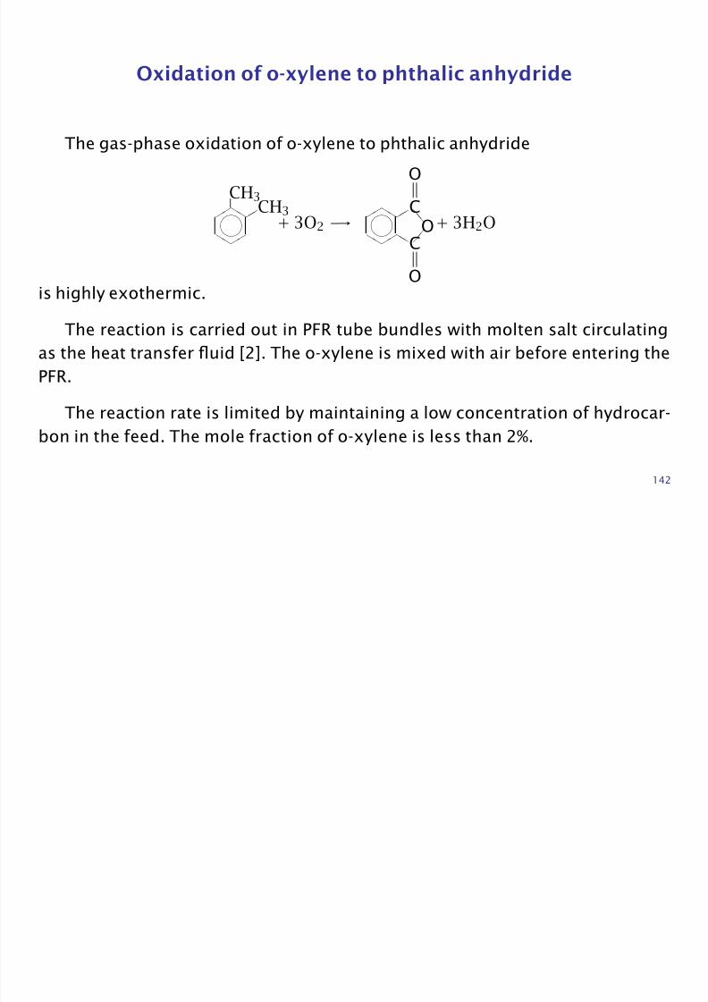
The gas-phase oxidation of o-xylene to phthalic anhydride
CH3
CH3
+ 3O2 →
OC
CO
O
+ 3H2O
is highly exothermic.
The reaction is carried out in PFR tube bundles with molten salt circulating
as the heat transfer fluid [2]. The o-xylene is mixed with air before entering the
PFR.
The reaction rate is limited by maintaining a low concentration of hydrocar-
bon in the feed. The mole fraction of o-xylene is less than 2%.
142

8/20/2019 Slides Enbal
http://slidepdf.com/reader/full/slides-enbal 143/182
Under these conditions, the large excess of oxygen leads to a pseudo-first-
order rate expression
r = km exp
−E
1
T −
1
T m
cx
in which cx is the o-xylene concentration.
The operating pressure is atmospheric.
Calculate the temperature and o-xylene composition profiles.
The kinetic parameters are adapted from Van Welsenaere and Froment and
given in Table 6 [8].
143

8/20/2019 Slides Enbal
http://slidepdf.com/reader/full/slides-enbal 144/182
Parameter Value Units
km 1922.6 s−1
T a 625 K
T m 625 K
P f 1.0 atm
l 1.5 m
R 0.0125 m
C p 0.992 kJ/kg KU o 0.373 kJ/m2 s K
y xf 0.019
E/R 1.3636 × 10⁴ K
∆H R −1.361 × 10³ kJ/kmol
Qρ 2.6371 × 10⁻³ kg/s
Table 6: PFR operating conditions and parameters for o-xylene example.
144
Solution

8/20/2019 Slides Enbal
http://slidepdf.com/reader/full/slides-enbal 145/182
If we assume constant thermochemical properties, an ideal gas mixture, andexpress the mole and energy balances in terms of reactor length, we obtain
dN x
dz = −Acr
dT
dz = −βr + γ(T a − T )
r = k P
RT
N xN
in which
β = ∆H RAc
QρC P
, γ = 2πRU o
QρC P
and the total molar flow is constant and equal to the feed molar flow because
of the stoichiometry.
145
Figure 27 shows the molar flow of o-xylene versus reactor length for several
values of the feed temperature The corresponding temperature profile is shown

8/20/2019 Slides Enbal
http://slidepdf.com/reader/full/slides-enbal 146/182
values of the feed temperature. The corresponding temperature profile is shown
in Figure 28.
146
2.0 × 10⁻⁶

8/20/2019 Slides Enbal
http://slidepdf.com/reader/full/slides-enbal 147/182
0
4.0 × 10⁻⁷
8.0 × 10⁻⁷
1.2 × 10⁻⁶
1.6 × 10⁻⁶
0 0.2 0.4 0.6 0.8 1 1.2 1.4
z (m)
N x
( k m o l / s )
615
620
625
T f = 630
Figure 27: Molar flow of o-xylene versus reactor length for different feed tem-
peratures.
147
740
Tf = 630

8/20/2019 Slides Enbal
http://slidepdf.com/reader/full/slides-enbal 148/182
600
620
640
660
680
700
720
0 0.2 0.4 0.6 0.8 1 1.2 1.4
z (m)
T (K)
615
620
625
T f = 630
Figure 28: Reactor temperature versus length for different feed temperatures.
148

8/20/2019 Slides Enbal
http://slidepdf.com/reader/full/slides-enbal 149/182
• We see a hotspot in the reactor for each feed temperature.
• Notice the hotspot temperature increases and moves down the tube as we
increase the feed temperature.
• Finally, notice if we increase the feed temperature above about 631 K, the
temperature spikes quickly to a large value and all of the o-xylene is converted
by z = 0.6 m, which is a classic example of reactor runaway.
• To avoid this reactor runaway, we must maintain the feed temperature below
a safe value.
• This safe value obviously also depends on how well we can control the com-
position and temperature in the feed stream. Tighter control allows us to
149
operate safely at higher feed temperatures and feed o-xylene mole fractions,
which increases the production rate.

8/20/2019 Slides Enbal
http://slidepdf.com/reader/full/slides-enbal 150/182
which increases the production rate.
150
The Autothermal Plug-Flow Reactor
8/20/2019 Slides Enbal
http://slidepdf.com/reader/full/slides-enbal 151/182
In many applications, it is necessary to heat a feed stream to achieve a reactor
inlet temperature having a high reaction rate.
If the reaction also is exothermic, we have the possibility to lower the reactor
operating cost by heat integration.
The essential idea is to use the heat released by the reaction to heat the
feed stream. As a simple example of this concept, consider the following heat
integration scheme
151

8/20/2019 Slides Enbal
http://slidepdf.com/reader/full/slides-enbal 152/182
Catalyst bed wherereaction occurs
Feed
ProductsPreheater
Reactants
Annulus in which feedis further heated
T af T a(l) = T af
T a(0) = T (0)
T a
T
Figure 29: Autothermal plug-flow reactor; the heat released by the exothermicreaction is used to preheat the feed.
152
8/20/2019 Slides Enbal
http://slidepdf.com/reader/full/slides-enbal 153/182
This reactor configuration is known as an autothermal plug-flow reactor.
The reactor system is an annular tube. The feed passes through the outer
region and is heated through contact with the hot reactor wall.
The feed then enters the inner reaction region, which is filled with the cata-
lyst, and flows countercurrently to the feed stream.
The heat released due to reaction in the inner region is used to heat the feed
in the outer region. When the reactor is operating at steady state, no external
heat is required to preheat the feed.
Of course, during the reactor start up, external heat must be supplied to
ignite the reactor.
153
The added complexity of heat integration

8/20/2019 Slides Enbal
http://slidepdf.com/reader/full/slides-enbal 154/182
Although recycle of energy can offer greatly lower operating costs, the dy-
namics and control of these reactors may be complex. We next examine an
ammonia synthesis example to show that multiple steady states are possible.
Ammonia synthesis had a large impact on the early development of the chem-
ical engineering discipline. Quoting Aftalion [1, p. 101]
154
Early Days of Chemical Engineering

8/20/2019 Slides Enbal
http://slidepdf.com/reader/full/slides-enbal 155/182
While physicists and chemists were linking up to understand the struc-
ture of matter and giving birth to physical chemistry , another discipline
was emerging, particularly in the United States, at the beginning of the
twentieth century, that of chemical engineering . . . it was undoubtedly the
synthesis of ammonia by BASF, successfully achieved in 1913 in Oppau,which forged the linking of chemistry with physics and engineering as it
required knowledge in areas of analysis, equilibrium reactions, high pres-
sures, catalysis, resistance of materials, and design of large-scale appara-
tus.
155
Ammonia synthesis

8/20/2019 Slides Enbal
http://slidepdf.com/reader/full/slides-enbal 156/182
Calculate the steady-state conversion for the synthesis of ammonia using the
autothermal process shown previously
A rate expression for the reaction
N2 + 3H2
k1 k−1
2NH3 (44)
over an iron catalyst at 300 atm pressure is suggested by Temkin [5]
r = k−1/RT
K 2(T )
P N P 3/2H
P A−
P A
P 3/2H
(45)
156
in which P N , P H , P A are the partial pressures of nitrogen, hydrogen, and ammo-
nia, respectively, and K is the equilibrium constant for the reaction forming one

8/20/2019 Slides Enbal
http://slidepdf.com/reader/full/slides-enbal 157/182
mole of ammonia.
For illustration, we assume the thermochemical properties are constant and
the gases form an ideal-gas mixture.
More accurate thermochemical properties and a more accurate equation of
state do not affect the fundamental behavior predicted by the reactor model.
The steady-state material balance for the ammonia is
dN AdV = RA = 2r
N A(0) = N Af
157

8/20/2019 Slides Enbal
http://slidepdf.com/reader/full/slides-enbal 158/182
Parameter Value Units
P 300 atm

8/20/2019 Slides Enbal
http://slidepdf.com/reader/full/slides-enbal 159/182
Q0 0.16 m3/s
Ac
1 m2
l 12 m
T af 323 K
γ = 2π RU o
QρC P
0.5 1/m
β = ∆H RAc
QρC P
−2.342 m2 s K/mol
∆G◦ 4250 cal/mol
∆H ◦ −1.2 × 10⁴ cal/mol
k−10 7.794 × 10¹¹
E −1/R 2 × 10⁴ K
Table 7: Parameter values for ammonia example
The material balances for the feed-heating section are simple because reac-
159
tion does not take place without the catalyst. Without reaction, the molar flow
of all species are constant and equal to their feed values and the energy balance

8/20/2019 Slides Enbal
http://slidepdf.com/reader/full/slides-enbal 160/182
for the feed-heating section is
QaρaC P adT adV a
= −q (47)
T a(0) = T af
in which the subscript a represents the fluid in the feed-heating section. Notice
the heat terms are of opposite signs in Equations 47 and 46. If we assume
the fluid properties do not change significantly over the temperature range of
interest, and switch the direction of integration in Equation 47 using dV a = −dV ,
we obtain
QρC P
dT adV = q (48)
T a(V R) = T af (49)
160
Finally we require a boundary condition for the reactor energy balance, which we
have from the fact that the heating fluid enters the reactor at z = 0, T (0) = T a(0).

8/20/2019 Slides Enbal
http://slidepdf.com/reader/full/slides-enbal 161/182
Combining these balances and boundary conditions and converting to reactor
length in place of volume gives the model
dN A
dz = 2Acr N A(0) = N Af
dT
dz
= −βr + γ(T a − T ) T (0) = T a(0)
dT adz
= γ(T a − T ) T a(l) = T af
(50)
in which
β =
∆H RAc
QρC P γ =
2π RU o
QρC P
Equation 50 is a boundary-value problem, rather than an initial-value prob-
161
lem, because T a is specified at the exit of the reactor. A simple solution strategy
is to guess the reactor inlet temperature, solve the model to the exit of the reac-

8/20/2019 Slides Enbal
http://slidepdf.com/reader/full/slides-enbal 162/182
tor, and then compare the computed feed preheat temperature to the specified
value T af . This strategy is known as a shooting method. We guess the missingvalues required to produce an initial-value problem. We solve the initial-value
problem, and then iterate on the guessed values until we match the specified
boundary conditions. We will see more about boundary-value problems and
shooting methods when we treat diffusion in Chapter 7.
162

8/20/2019 Slides Enbal
http://slidepdf.com/reader/full/slides-enbal 163/182
600
700

8/20/2019 Slides Enbal
http://slidepdf.com/reader/full/slides-enbal 164/182
0
100
200
300
400
500
600
200 300 400 500 600 700 800 900 1000
T a(0)(K)
T (K)• • •
A B C
T af
T a(l)
Figure 30: Coolant temperature at reactor outlet versus temperature at reactor
inlet, T a(l) versus T a(0); intersection with coolant feed temperature T af indi-
cates three steady-state solutions (A,B,C).
164
Solution

8/20/2019 Slides Enbal
http://slidepdf.com/reader/full/slides-enbal 165/182
The profiles in the reactor for these three steady states are shown in Fig-
ures 31 and 32. It is important to operate at the upper steady state so that a
reasonably large production of ammonia is achieved.
165

8/20/2019 Slides Enbal
http://slidepdf.com/reader/full/slides-enbal 166/182
300
400
500
600
700
800
900
1000
0 2 4 6 8 10 12
z (m)
T , T a
T a
T
T a
T
A
B
C
T (K)
Figure 31: Reactor and coolant temperature profiles versus reactor length; lower
(A), unstable middle (B), and upper (C) steady states.
166
0.25

8/20/2019 Slides Enbal
http://slidepdf.com/reader/full/slides-enbal 167/182
0
0.05
0.1
0.15
0.2
0 2 4 6 8 10 12
z (m)
xA
A
B
C
Figure 32: Ammonia mole fraction versus reactor length; lower (A), unstable
middle (B), and upper (C) steady states.
167
Summary

8/20/2019 Slides Enbal
http://slidepdf.com/reader/full/slides-enbal 168/182
• Tables 8–11 summarize the important energy balances for the batch,
continuous-stirred-tank, semi-batch, and plug-flow reactors.
• In contrast to the material balance, which is reasonably straightforward,
choosing the proper energy balance requires some care. It is unwise to select
an energy balance from a book without carefully considering the assumptions
that have been made in the derivation of that particular energy balance.
• Hopefully these tables will help you to choose an appropriate energy balance.
168
Neglect kinetic and potential energiesdU
dt = Q + W s + W b

8/20/2019 Slides Enbal
http://slidepdf.com/reader/full/slides-enbal 169/182
Neglect shaft workdU
dt
+ P dV R
dt
= Q
dH
dt − V R
dP
dt = Q
Single phase
V RρC P dT
dt − αT V R
dP
dt +
j
H j
dnj
dt = Q
V
R
ρC
P
dT
dt
− αT V
R
dP
dt
= −i
∆H
Ri
r
i
V
R
+ Q
a. Incompressible-fluid or constant-pressure reactor
V RρC P dT
dt = −
i
∆H Rir iV R + Q
169
b. Constant-volume reactor
ˆdT
∂P
˙

8/20/2019 Slides Enbal
http://slidepdf.com/reader/full/slides-enbal 170/182
V RρC V dT
dt = −
i
∆H Ri − αT V R
j
νij
∂P
∂nj
T,V,nk
r iV R + Q
b.1 Constant-volume reactor, ideal gas
V RρC V dT
dt = −
i
∆H Ri − RT νi
r iV R + Q
Table 8: Energy balances for the batch reactor.
170
Neglect kinetic and potential energiesdU
dt = Qf ρf
H f − Qρ H + Q + W s + W b (51)
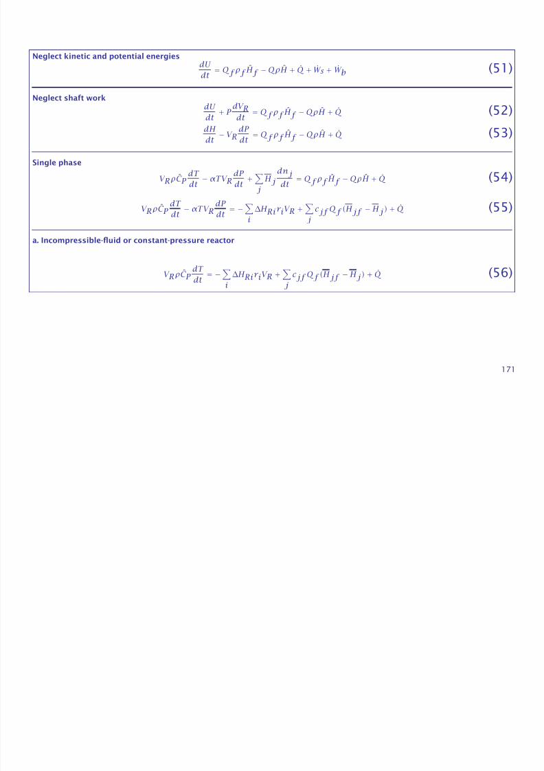
8/20/2019 Slides Enbal
http://slidepdf.com/reader/full/slides-enbal 171/182
Neglect shaft workdU
dt + P
dV R
dt = Qf ρf ˆH f − Qρ
ˆH +
˙Q (52)
dH
dt − V R
dP
dt = Qf ρf
H f − Qρ H + Q (53)
Single phase
V RρC P dT
dt − αT V R
dP
dt +
j
H j
dnj
dt = Qf ρf
H f − Qρ H + Q (54)
V RρC P
dT
dt − αT V R
dP
dt = −i∆H Rir iV R +
j
cjf Qf (H jf − H j ) + Q (55)
a. Incompressible-fluid or constant-pressure reactor
V RρC P dT
dt = −
i
∆H Rir iV R +j
cjf Qf (H jf − H j) + Q (56)
171
b. Constant-volume reactor
V RρC VdT
dt = −
∆H Ri − αT V R
νij P nj
r iV R +
cjf Qf (H jf − H j) + αT V R
P nj
(cjf Qf − cjQ) + Q (57)

8/20/2019 Slides Enbal
http://slidepdf.com/reader/full/slides-enbal 172/182
Rρ V dt
i
Ri R
j
ij nj
i R
j
jf Qf ( jf j) Rj
nj( jf Qf jQ) Q (5 )
b.1 Constant-volume reactor, ideal gas
V RρC V dT
dt = −
i
∆H Ri − RT νi
r iV R +
j
cjf Qf (H jf − H j) + RT j
(cjf Qf − cj Q) + Q (58)
c. Steady state, constant C P , P = P f
−i
∆H Rir iV R + Qf ρf C P (T f − T ) + Q = 0 (59)
Table 9: Energy balances for the CSTR.
172
Neglect kinetic and potential energiesdU
dt = Qf ρf
H f + Q + W s + W b (60)

8/20/2019 Slides Enbal
http://slidepdf.com/reader/full/slides-enbal 173/182
Neglect shaft workdU
dt + P
dV R
dt = Qf ρf ˆH f +
˙Q (61)
dH
dt − V R
dP
dt = Qf ρf
H f + Q (62)
Single phase
V RρC P dT
dt − αT V R
dP
dt +
j
H j
dnj
dt = Qf ρf
H f + Q (63)
V RρC P
dT
dt − αT V R
dP
dt = −i∆H Rir iV R +
j
cjf Qf (H jf − H j ) + Q (64)
a. Incompressible-fluid or constant-pressure reactor
V RρC P dT
dt = −
i
∆H Rir iV R +j
cjf Qf (H jf − H j) + Q (65)
a.1 Constant C P
V RρC P dT
dt = −
i
∆H Rir iV R + Qf ρf C P (T f − T ) + Q (66)
Table 10: Energy balances for the semi-batch reactor. 173
Neglect kinetic and potential energies and shaft work
∂(ρU) =
1 ∂(QρH) + q (67)

8/20/2019 Slides Enbal
http://slidepdf.com/reader/full/slides-enbal 174/182
∂t(ρU) = −
Ac ∂z(Qρ H) + q (67)
Heat transfer with an overall heat-transfer coefficient
q = 2
RU o(T a − T ) (68)
Steady stated
dV (Qρ H) = q (69)
Single phase
QρC P dT
dV + Q(1 − αT )
dP
dV = −
i
∆H Rir i + q (70)
a. Neglect pressure drop, or ideal gas
QρC P dT dV
= −i
∆H Rir i + q (71)
b. Incompressible fluid
QρC P dT
dV + Q
dP
dV = −
i
∆H Rir i + q (72)
Table 11: Energy balances for the plug-flow reactor.
174
Summary

8/20/2019 Slides Enbal
http://slidepdf.com/reader/full/slides-enbal 175/182
• Nonisothermal reactor design requires the simultaneous solution of the ap-propriate energy balance and the species material balances. For the batch,
semi-batch, and steady-state plug-flow reactors, these balances are sets of
initial-value ODEs that must be solved numerically.
• In very limited situations (constant thermodynamic properties, single reac-tion, adiabatic), one can solve the energy balance to get an algebraic relation
between temperature and concentration or molar flowrate.
• The nonlinear nature of the energy and material balances can lead to multi-
ple steady-state solutions. Steady-state solutions may be unstable, and the
reactor can exhibit sustained oscillations. These reactor behaviors were il-
lustrated with exothermic CSTRs and autothermal tubular reactors.
175
Notation

8/20/2019 Slides Enbal
http://slidepdf.com/reader/full/slides-enbal 176/182
A heat transfer area
Ac reactor tube cross-sectional area
Ai preexponential factor for rate constant i
cj concentration of species j
cjf feed concentration of species j
cjs steady-state concentration of species j
cj0 initial concentration of species j
C P constant-pressure heat capacity
C P j partial molar heat capacity
C P s heat capacity per volume
C P constant-pressure heat capacity per massC V constant-volume heat capacity per mass
∆C P heat capacity change on reaction, ∆C P =
j νjC Pj
176
E i activation energy for rate constant i
E k total energy of stream k
Ek total energy per mass of stream k
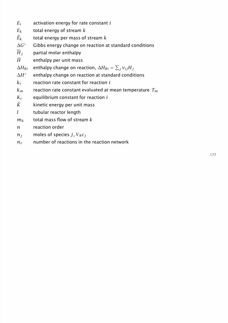
8/20/2019 Slides Enbal
http://slidepdf.com/reader/full/slides-enbal 177/182
E k total energy per mass of stream k
∆G◦ Gibbs energy change on reaction at standard conditions
H j partial molar enthalpy
H enthalpy per unit mass
∆H Ri enthalpy change on reaction, ∆H Ri =
j νijH j
∆H ◦ enthalpy change on reaction at standard conditions
ki reaction rate constant for reaction i
km reaction rate constant evaluated at mean temperature T m
K i equilibrium constant for reaction i
K kinetic energy per unit mass
l tubular reactor length
mk total mass flow of stream k
n reaction ordernj moles of species j , V Rcj
nr number of reactions in the reaction network
177
ns number of species in the reaction network
N j molar flow of species j , Qcj
Njf feed molar flow of species j , Qcj

8/20/2019 Slides Enbal
http://slidepdf.com/reader/full/slides-enbal 178/182
N jf feed molar flow of species j , Qcj
P pressure
P j partial pressure of component j
P nj P nj
= (∂P/∂nj)T,V,nk
q heat transfer rate per volume for tubular reactor, q = 2R U o(T a − T )
Q volumetric flowrate
Qf feed volumetric flowrate
Q heat transfer rate to reactor, usually modeled as Q = U oA(T a − T )
r i reaction rate for ith reaction
r tot total reaction rate,
i r i
R gas constant
Rj production rate for j th species
t timeT temperature
T a temperature of heat transfer medium
178
T m mean temperature at which k is evaluated
U o overall heat transfer coefficient
U internal energy per mass

8/20/2019 Slides Enbal
http://slidepdf.com/reader/full/slides-enbal 179/182
U internal energy per mass
vk velocity of stream k
V reactor volume variable
V j partial molar volume of species j
V ◦j specific molar volume of species j
V R reactor volume
∆V i change in volume upon reaction i, j νijV j
W rate work is done on the system
xj number of molecules of species j in a stochastic simulation
xj molar conversion of species j
y j mole fraction of gas-phase species j
z reactor length variable
α coefficient of expansion of the mixture, α = (1/V)(∂V/∂T)P ,nj
εi extent of reaction i
τ reactor residence time, τ = V R/Qf
179
νij stoichiometric coefficient for species j in reaction i
νi
j νij
ρ mass density

8/20/2019 Slides Enbal
http://slidepdf.com/reader/full/slides-enbal 180/182
ρ y
ρk mass density of stream k
Φ potential energy per mass
180
References

8/20/2019 Slides Enbal
http://slidepdf.com/reader/full/slides-enbal 181/182
[1] F. Aftalion. A History of the International Chemical Industry . Chemical Her-
itage Press, Philadelphia, second edition, 2001. Translated by Otto Theodor
Benfey.
[2] G. F. Froment and K. B. Bischoff. Chemical Reactor Analysis and Design.
John Wiley & Sons, New York, second edition, 1990.
[3] L. S. Henderson. Stability analysis of polymerization in continuous stirred-
tank reactors. Chem. Eng. Prog., pages 42–50, March 1987.
[4] K. S. Pitzer. Thermodynamics . McGraw-Hill, third edition, 1995.
[5] M. Temkin and V. Pyzhev. Kinetics of ammonia synthesis on promoted iron
catalysts. Acta Physicochimica U.R.S.S., 12(3):327–356, 1940.
181
[6] A. Uppal, W. H. Ray, and A. B. Poore. On the dynamic behavior of continuous
stirred tank reactors. Chem. Eng. Sci., 29:967–985, 1974.

8/20/2019 Slides Enbal
http://slidepdf.com/reader/full/slides-enbal 182/182
[7] C. van Heerden. Autothermic processes. Properties and reactor design. Ind.Eng. Chem., 45(6):1242–1247, 1953.
[8] R. J. Van Welsenaere and G. F. Froment. Parametric sensitivity and runaway
in fixed bed catalytic reactors. Chem. Eng. Sci., 25:1503–1516, 1970.