small area estimation of sub-national poverty...

Small Area Estimation of Sub-National Poverty Incidence1

by

ZITA VILLA JUAN-ALBACEA, Ph.D.2 I. INTRODUCTION Poverty monitoring needs statistics generated at a regular unit of time and for a particular domain of study. Most of the time, the policy makers who use such statistics need these values annually. More so, they need the statistics of a domain of study small enough to be able to target the right group. Like in any other countries, the Philippines monitors the poverty situation using official poverty statistics. The National Statistics Coordination Board (NSCB) is the agency mandated to release these official poverty statistics. Usually, NSCB releases the official statistics that were declared reliable to be used for the purpose of monitoring poverty.

Official poverty statistics are computed from a nation wide survey conducted by the National Statistics Office. Most of the nation wide surveys are conducted with large area like a region as domain of estimation. In the year 2000, there are sixteen (16) regions in the Philippines and a region is composed of several provinces. There are a total of 82 provinces in the country. The number of geographical divisions like regions and provinces continue to change as political environment in the country changes.

Another political change occurred in the country led to the strengthening of the local government through the devolution of functions and power to the local government units. This change in focus shifts the demand of official statistics from the regional level to the level of local units. More administrators or policy makers demand for statistics at the local area. They said that such statistics are more useful to them specially in planning government programs to better serve their constituents.

Provincial or even smaller geographical division poverty statistics are needed to

better implement, monitor and evaluate projects. The national government, on the other hand, uses these statistics to determine specific provinces or municipalities that need more 1 A paper presented at the ADB-GTZ-CEPA Regional Conference on Poverty Monitoring, ADB Headquarters, Manila, Philippines, March 24-26, 2004. This paper was developed mostly from the results of two studies entitled “Targeting the Poor in the Philippines” and “Estimating Philippine Provincial Poverty Incidence Using Administrative Data, conducted by the author under the ADB Technical Assistance 3656 PHI: Improving Poverty Monitoring Surveys, with the National Statistics Office, Philippines as implementing agency. 2 Associate Professor of Statistics, and currently, Vice-Chancellor for Administration, University of the Philippines Los Baños, College, Laguna, Philippines.

Small Area Estimation of Sub-National Poverty Incidence by Zita Villa Juan-Albacea, Ph.D.

government support. The provinces are ranked according to their poverty incidences and the top 44 poorest provinces are given government support. Hence, it is important to have reliable poverty incidence measures so that valid rankings of provinces can also be attained. In this way the provinces that really need support from the government will be correctly identified.

The Family Income and Expenditure Survey (FIES), one of the nationwide surveys, is

the source of official poverty statistics. FIES is conducted every three years with about 41,000 sample households. The most recent survey was conducted during the year 2000 and it made use of provinces and key cities as domains. The 2000 FIES is the second time the survey was conducted based on the revised master plan of households that took effect last 1997. The survey used the master sample that was designed to provide estimates at the provincial level with an acceptable measure of reliability. However, some of the resulting estimates at the provincial level did not render sampling errors at tolerable level.

Since poverty statistics at provincial level are used by Department of Social Welfare

and Development (DSWD) and National Anti-Poverty Commission (NAPC) to allocate funds for poverty alleviation programs, having some unstable estimates at the provincial level may cause inappropriate choices of target areas for these programs and projects. Therefore, there is a need to further improve the estimates at the provincial level. One way to do this is to draw additional sample households for each province. The result of investigation by National Statistics Office (NSO) following this scenario indicates that the sample households need to be increased four times the current sample size allocation by province (NSO, 2003). Roughly, this would also require four times the current budget allocation for FIES. Moreover, non-sampling errors may increase because with the increase in sample size, the number of enumerators and supervisors also have to be enlarged and the quality of their work may not be maintained.

Another alternative approach to get reliable provincial level statistics without increasing the cost of the survey and risking the increase of non-sampling error is to use small area estimation techniques. This paper will discuss the results of two studies conducted under the Asian Development Bank Technical Assistance 3656 PHI: Improving Poverty Monitoring Surveys that aim to examine various small area estimation techniques that could be applied to the existing data sets in the Philippine Statistical System to generate sub-domain level estimates. The next section of this paper will discuss the design-based estimates of the Philippine provincial poverty incidence and its properties. The poverty situation in the different provinces of the Philippines will be described using the results of the design-based estimation procedure. Section III gives a brief background of some small area estimation techniques as applied to poverty studies while Section IV describes the proposed procedure to be used in estimating provincial poverty incidence. The results of the proposed methodology as applied to the Philippine situation are presented in Section V. The lessons learned in doing this research work are presented in Section VI. In Section VII, the paper ends by giving more specific applications and further improvements of the methodology presented.


II. DESIGN-BASED ESTIMATES OF POVERTY INCIDENCE: Poverty incidence is a ratio of the total number of poor households with the total number of households. A poor household is defined as a household whose per capita income is below the regional poverty threshold.

With the province as small area unit, the provincial proportions of poor households or commonly referred to as provincial poverty incidences are estimated using the 2000 FIES data set. These estimates are referred to as design-based estimates as these were computed based on the sampling design of the survey.

The national estimate of poverty incidence in the Philippines based on the 2000 FIES

data is 33.6% with 0.004 standard error. This estimate has a coefficient of variation equal to 1.2%. Such estimate is precise with a 95% confidence interval estimate from 32.8% to 34.5% of households in the Philippines are said to be poor. It is estimated that one-third of the households in the Philippines or around 3 for every 10 households are poor.

The regional poverty incidence estimates obtained using the 2000 FIES data set are given in Table 1. The poorest region is Region 15 or the Autonomous Region of Muslim Mindanao (ARMM) with an estimated 66% poverty incidence and standard error of 0.023 while the region with the smallest poverty incidence is the National Capital Region (NCR) or Region 13 with an estimated poverty incidence of 8.7%. This estimate has standard error of 0.006. Table 1. Design-based estimates of regional poverty incidence, 2000 FIES.

Region

Name

Poverty incidence estimate

(%)

Standard error of the

estimate

95% Confidence interval estimates

(%)

Coefficient of variation

(%) 1 Ilocos Region 37.1 0.016 34.1 - 40.2 4.3 2 Cagayan Valley 29.5 0.022 25.2 – 33.7 7.5 3 Central Luzon 18.6 0.011 16.6 – 20.7 5.9 4 Southern Tagalog 25.3 0.011 23.2 – 27.4 4.3 5 Bicol Region 55.4 0.018 51.9 - 58.9 3.2 6 Western Visayas 43.1 0.013 40.5 – 45.6 3.0 7 Central Visayas 38.8 0.019 35.1 – 42.4 4.9 8 Eastern Visayas 43.6 0.022 39.2 – 47.9 5.0 9 Western Mindanao 46.6 0.023 42.1 – 51.2 4.9

10 Northern Mindanao 43.1 0.021 38.9 – 47.3 4.9 11 Southern Mindanao 39.2 0.021 35.2 – 43.2 5.4 12 Central Mindanao 51.1 0.022 46.8 – 55.3 4.3 13 National Capital Region 8.7 0.006 7.0 - 9.9 6.9 14 Cordillera Autonomous

Region 36.6 0.017 33.3 – 39.9 4.6

15 Autonomous Region of Muslim Mindanao

66.0 0.023 61.4 – 70.5 3.5

16 CARAGA 49.4 0.021 45.3 – 53.4 4.2


Table 1 also gives the 95% confidence interval estimates for the 16 regions in the

country, the standard error and corresponding coefficients of variation of the design-based regional estimates. The distances measured in the interval estimates are at most 9.1% while the minimum is 2.9%. Large distances were observed for estimates with high standard errors relative to other regional estimates like in Regions 2, 8, 9 10, 11, 12, 15 and 16. However, the values of the coefficient of variation are all less than 10%. These reported values indicate that the design-based estimates of regional poverty incidence obtained are reliable. The direct or design-based estimates of the provincial poverty incidence range from 5% (Batanes) up to 72.7% (Sulu) (see Appendix Table 1). The design-based estimate for the province of Batanes has a standard error of 0.03 with a high coefficient of variation equal to 60.9%. A 95% confidence interval estimate of poverty incidence for the province of Batanes is from –1.1% to 11.1%. Having a negative estimate of poverty incidence is questionable. On the other hand, for the province of Sulu, the 95% confidence interval estimate of its poverty incidence is from 63.1% to 82.2%.

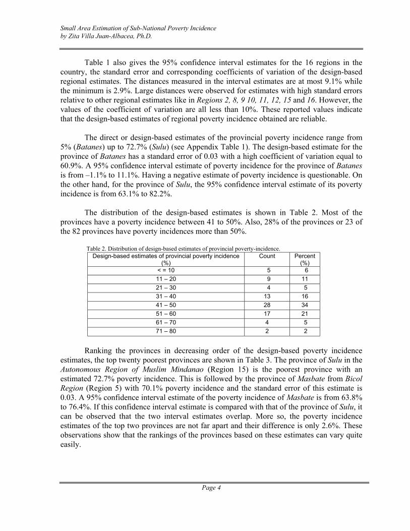
The distribution of the design-based estimates is shown in Table 2. Most of the provinces have a poverty incidence between 41 to 50%. Also, 28% of the provinces or 23 of the 82 provinces have poverty incidences more than 50%.

Table 2. Distribution of design-based estimates of provincial poverty-incidence. Design-based estimates of provincial poverty incidence

(%) Count Percent

(%) < = 10 5 6 11 – 20 9 11 21 – 30 4 5 31 – 40 13 16 41 – 50 28 34 51 – 60 17 21 61 – 70 4 5 71 – 80 2 2

Ranking the provinces in decreasing order of the design-based poverty incidence

estimates, the top twenty poorest provinces are shown in Table 3. The province of Sulu in the Autonomous Region of Muslim Mindanao (Region 15) is the poorest province with an estimated 72.7% poverty incidence. This is followed by the province of Masbate from Bicol Region (Region 5) with 70.1% poverty incidence and the standard error of this estimate is 0.03. A 95% confidence interval estimate of the poverty incidence of Masbate is from 63.8% to 76.4%. If this confidence interval estimate is compared with that of the province of Sulu, it can be observed that the two interval estimates overlap. More so, the poverty incidence estimates of the top two provinces are not far apart and their difference is only 2.6%. These observations show that the rankings of the provinces based on these estimates can vary quite easily.


Table 3. Top twenty poorest provinces based on the design-based estimates.

Code

Rank

Province name

Poverty incidence

(%)


estimate


(%)


(%) 66 1 Sulu 72.7 0.048 63.1 - 82.2 6.5 41 2 Masbate 70.1 0.032 63.8 - 76.4 4.5 59 3 Romblon 69.3 0.035 62.4 - 76.3 5.0 38 4 Maguindanao 67.8 0.036 60.7 - 74.9 5.2 27 5 Ifugao 67.1 0.047 57.8 - 76.5 6.9 70 6 Tawi Tawi 65.3 0.058 53.8 - 76.8 8.8 16 7 Camarines Norte 58.1 0.056 47.0 - 69.3 9.6 36 8 Lanao del Sur 57.1 0.052 46.7 - 67.5 9.1 65 9 Sultan Kudarat 57.0 0.052 46.7 - 67.4 9.1 3 10 Agusan del Sur 56.2 0.050 46.1 - 66.2 9.0 42 11 Misamis Occidental 55.9 0.038 48.3 - 63.5 6.8 12 12 Bohol 55.6 0.044 46.8 - 64.3 7.9 51 13 Occidental Mindoro 55.4 0.035 48.5 - 62.3 6.2 40 14 Marinduque 54.6 0.035 47.7 - 61.6 6.4 80 15 Sarangani 54.5 0.092 36.1 - 72.9 16.9 18 16 Camiguin 54.2 0.057 42.8 - 65.6 10.5 26 17 Eastern Samar 53.2 0.038 45.6 - 60.8 7.2 19 18 Capiz 52.7 0.039 44.9 - 60.6 7.5 1 19 Abra 52.4 0.038 44.7 - 60.0 7.3 72 20 Zamboanga del Norte 51.7 0.057 40.2 - 63.1 11.1

The poverty incidence estimates of these twenty poorest provinces are close to each other ranging from 51.7% to 72.7%. The estimate with the highest standard error (0.092) is the province of Sarangani. Having a high standard error leads to a wide 95% confidence interval estimate, from 36.1% up to 72.9%. Such interval estimate is so wide that it gives the possibility that the true value of the poverty incidence for this province may be as high as 72.9%. With such estimate, Sarangani can be declared as the poorest province where in fact it ranks only15th poorest province. There is also possibility that the province will be found in the bottom 28 richest province if the lower bound of the 95% confidence interval estimate is considered. This means that the ranking of the provinces may greatly change especially if there are many provinces with wider confidence intervals. High value of coefficient of variation also indicates unreliable estimate. Among the top twenty poorest provinces, 3 estimates have coefficients of variation greater than 10%. The estimate with the highest coefficient of variation is that of the province of Sarangani which has also the largest standard error. This further shows that the poverty incidence estimate of Sarangani is indeed unreliable.

Further, Appendix Table 1 shows that the highest coefficient of variation is 60.9% from the estimate for the province of Batanes (Rank = 82, Code = 9) while the lowest is 4.5% from the province of Masbate (Rank = 21, Code = 41). The number of sampled households in Batanes is 95 while 379 households were sampled from Masbate. The small


sample size for the province of Batanes may have contributed to the high coefficient of variation of its estimate.

Deleting the extreme value of 60.9%, the distribution of the coefficients of variation of the remaining 81 provinces is shown in Table 4. Fifty percent of the coefficients have values at most 10% and the remaining half of the distribution exceeding the 10% acceptable value of the coefficient of variation. This observation indicates that some of the provincial poverty incidence estimates specifically those with high coefficients of variation are not precise, hence are not reliable to use. However such estimates can still be improved using a different estimation technique.

Table 4. Distribution of the coefficient of variation of the design-based estimates of provincial poverty incidence.

Coefficient of variation of the design-based estimates of provincial poverty incidence

(%)

Count

Percent

< = 10 41 50 11 – 20 39 48 21 – 30 1 1

III. SMALL AREA ESTIMATION TECHNIQUE There are many small area estimation techniques that have been developed. One approach is to use synthetic or indirect estimation procedure. This procedure is called indirect since the estimates are not directly obtained from survey data. Synthetic estimation makes use of information from similar small areas. This procedure assumes that the small areas have same characteristics of a larger domain to which the small areas belong. The initial application of this technique was done by the National Center for Health Statistics in 1968. In 1977, Nichol proposes to add the synthetic estimate as an additional independent variable in sample-regression method, another small area estimation technique. This small area estimation technique makes use of regression model to predict the variable of interest.

In one of the studies conducted by Siegel in 1995 for the U.S. Census Bureau, the procedure provides postcensal estimates of income and poverty for small area during the 1990’s. The estimation aims to estimate income and poverty for counties biennially with the initial estimates for calendar (income) year 1993 and released in late 1996. The six key statistics include median household income, per capita income and number of poor persons and poverty rates for four groups, namely; the total population, children age 5 to 17, children under age five and persons age 65 and over.

Siegel also suggested two strategies for postcensal sub-state income and poverty

estimation. The first approach is to estimate postcensal change in poverty from postcensal change in the indicators by assuming that the relation between changes in two series is the


same in the postcensal period as it was in the preceding intercensal period. However, the period from 1980 to 1990 experienced massive changes in the tax code which makes it unreliable to assume that the relation between 1980 and 1990 intercensal change in poverty and change in the tax data is the same as the postcensal relation between changes in tax and poverty data after 1990. An alternative is to take the ratio of the direct CPS estimate of a small area to that of the census value as dependent variable. Regressing that share change ratio on a similar ratio of one or more auxiliary variables provides a ‘ratio-regression model’.

The second approach is to have an estimator, which relies entirely in cross sectional

relations. This cross-sectional estimator has the advantages that it can be used to make estimates in any year for which CPS and tax data are available. Also, it should be less disastrously affected by changes in the tax laws. In this study, the model building process is incorporated in the methodology.

Other similar studies make use of model-based approach in small area estimation. A

World Bank study conducted by Lanjouw, et. al. in 1999, developed a predicting model for household consumption using survey data. The resulting predicting model is then applied to the census data to obtain poverty statistics of small area which when obtained directly from survey data will result to estimates with large standard errors. The study illustrated the use of model-based approach in estimating poverty statistics of small areas.

Another approach, which is more acceptable to a wider group of users, is to combine the model-based and the design-based estimation procedures. This approach was used by the U.S. Census Bureau’s Small Area Income and Poverty Estimates (SAIPE) Program in the early 1990s to provide estimates that would be more timely than those from the decennial census. The SAIPE estimates are developed by using a variety of data sources. A model was developed from the data that are obtained from several sources and this model is used to predict state poverty or income. The regression predictions are then combined with the corresponding direct estimates using a procedure in which the weights given to the predicted values and the direct estimates depend on their relative precision (National Research Council, 2000). The estimates obtained from combining the model- and design-based estimates are known in literature as the empirical best linear unbiased prediction (EBLUP) estimates. The EBLUP estimates are said to have the good properties of both the design- and model-based estimates.

The EBLUP estimation procedure starts with finding correlates or indicators of the

statistic to be predicted. In this case, it is poverty incidence. The survey data are used to identify these correlates. The correlates of poverty serve as pool of possible predictors in the model building process. The values of these predictors at the provincial level are then obtained from the census and administrative data sources.

The survey data set is used to obtain the design-based provincial estimates of poverty

incidence and its corresponding standard errors. Using the design-based estimate as dependent variable and the identified possible predictors, a predicting model is then


constructed. The best predicting model is chosen and used to predict the provincial poverty incidence. Also, an estimate of the error due to the modeling process is computed.

The EBLUP estimate is a weighted combination of the design- and model-based

estimates where the weights used based on the estimates of variability due to sampling process and the one due to modeling process. The design-based estimate is favored when the variability due to the modeling process is large. On the other hand, the model-based estimate is given more weight when the estimate of the sampling error is large. IV. METHODOLOGY THAT WAS USED

For the studies that were conducted under TA 3656 PHI, the methodology that was followed and being presented in this paper was the EBLUP estimation procedure, which is similar to the procedure used by SAIPE program and described in the previous section. The details of the application of the procedure are described in this section.

Sources of Data

There are three major sources of data for this study, namely; the Family Income and Expenditure Survey (FIES), Census of Population and Housing (CPH) and the administrative data sources. The survey data items of FIES, in addition to income and expenditure related variables, include characteristics of the household head and household characteristics that are also measured in the CPH.

The CPH is designed to take an inventory of the total population and housing units in the Philippines and to gather information about their characteristics. The census of population is the source of data on the size and distribution of the population as well as data on the demographic, social, economic and cultural characteristics. On the other hand, the census of housing provides data on the supply of housing units, their structural characteristics and facilities which have bearing on the maintenance of health and the development of normal household living conditions. As mentioned earlier, some of these data items are similar to those found in the FIES. However, it should be noted that the CPH data set does not include information on household income nor on expenditure. The variables that are common to both FIES and CPH are used to identify the possible correlates of poverty incidence. Specifically, the FIES data on these common variables are used to identify predictors of a model for provincial poverty incidence. These common variables are as follows: 1. sex of the household head 2. age of the household head 3. marital status of the household head 4. highest educational attainment of the household head


5. urban-rural place of usual residence 6. building type of the housing unit 7. construction material of the housing unit's roof 8. construction material of the housing unit's walls

9. floor area of the housing unit 10. tenure status of the lot where the housing unit is found 11. age composition of the household members

On the other hand, the characteristics of the barangays as taken in the CPH served as

indicators of the living conditions of the households within the community. These characteristics were then correlated to the poverty status of the household. The correlates served as basis in constructing indices which are also possible predictors of the model to be constructed.

Administrative data sets can be obtained from local government units, government

agencies and other units/agencies that collect data for other purposes. However, it should be noted that administrative data should be observed or measured consistently across the provinces. In this way, quality administrative data will be obtained. Administrative records are good data sources during the years when census is not conducted. The model with data coming from administrative data sources is still relevant even without the census data. Some of the potential sources of administrative data include the Department of Interior and Local Government, Department of Education, Bureau of Internal Revenue and the Local Government Units.

EBLUP Estimation of Provincial Poverty Incidence

In the model to be fitted, provincial poverty incidence is considered as the variable of interest or the variable whose values are to be predicted and the independent variables or predictors are the indices constructed based on the identified correlates of poverty. Using the 2000 Census of Population and Housing (CPH), the values of these indices at the provincial level were obtained and are defined as follows:

1. Proportion of the total provincial population whose household head is married male person and had reached at most secondary education.

2. Proportion of the total provincial population who are living in other structures not

intended for human habitation such as like boats and caves.

3. Proportion of the total provincial population who are living in housing units whose roofs and walls are constructed from light or makeshift or salvaged materials.

4. Proportion of the total provincial population who are living in housing units located in a rented lot.


5. Proportion of the total provincial population who are living in housing units with at

most 10 square meters floor area.

6. Proportion of the total provincial population who are living in barangays without a town hall or a college or university or public library or hospital or telegraph or with the surroundings as their waste disposal system.

7. Proportion of the total provincial population who are living in barangays with less

than 10 units of establishments in manufacturing sector or repair shops or restaurants or hotels or recreational establishments or banking or other financial institutions.

8. Proportion of the total provincial population who are living in barangays with more

than 50% of its residents who are engaged in agriculture.

To construct an index, a value of one (1) is given to a household satisfying a characteristic, like having a household head who is male married person and who had reached at most secondary education. Otherwise, the household will be assigned a value zero (0). This process results to an indicator variable having only two values, 1 and 0. The indicator variable is then weighted according to the number of household members by multiplying the indicator variable by the number of members the household has. The product will then be added for the whole province. The resulting sum is said to be the total number of household members who had the specified characteristic. Finally, the index is computed as the proportion of this total number over the total provincial population.

Several possible predictors of poverty incidence coming from administrative data sets were identified. From the Department of Education, the enrolment data during the school year 2000-2001 on elementary and secondary education, and both on the public and private schools were obtained. The data aggregated at the provincial level were used and the following possible predictors of provincial poverty incidence were identified:

1. Total enrolment of public schools in the elementary education, 2. Total enrolment of private schools in the elementary education, 3. Total enrolment of public schools in the secondary education, and 4. Total enrolment of private schools in the secondary education.

From the local government units, the number of building permits applied for

construction in the provinces is also a potential indicator of the poverty situation the province. Having large number of construction projects in the area also indicate good economic condition of the province since there is development in the area. The following are the provincial data taken in the year 2000:

1. Total number of building permits applied for residential purposes, 2. Reported area of the residential unit being constructed,


3. Reported total cost of construction of the residential unit, 4. Total number of building permits applied for non-residential units, 5. Reported area of the non-residential unit being constructed, and 6. Reported total cost of construction of the non-residential unit,

Also, from the local government the total population, total number of households,

total number of barangays and total area coverage of a province are also available. From these information several indicators were identified as follows:

1. annual population growth, 2. dependency ratio, 3. average household size, and 4. population density.

The Bureau of Internal Revenue is another government agency where administrative

data can also be obtained. The economic condition of a province can also be measured by its annual growth rate in internal revenue allotment and revenue collections. A more progressive province has a higher growth rate in its internal revenue allotment and revenue collections.

The Commission on Audit provides the annual provincial expenditures according to

its purpose. Expenditures on social services as percent of the total provincial expenditure indicate the amount the local government allocated for its social program rendered to its constituents. The model building process identifies the predictors for provincial poverty incidence. Internal diagnostics of the predicting model was conducted. Checks on the validity of the assumptions of the classical regression model were implemented to ensure good predicting model. The ordinary least squares (OLS) estimation procedure was first used to estimate the parameters of the model. Using these OLS estimates, the model weights are computed and used in refitting the model but this time using the weighted least squares estimation procedure. The resulting model is used to predict the provincial poverty incidences, which are referred to as model-based provincial poverty incidence estimates. The design- and model-based provincial poverty incidence estimates are then combined to form the EBLUP estimates. The weight used in combining the design- and model-based estimates is a ratio of the estimated variance due to modeling process over total variability. The sum of the estimated variances due to sampling and modeling process is an estimate of the total variability. V. RESULTS:

Several functional forms were tried but the simplest and most parsimonious model was chosen. The resulting predicting model for the provincial poverty incidence is composed of five predictors, namely; proportion of provincial population whose household head is a


married male person and had reached at least secondary education, provincial dependency ratio, provincial population density, average household size of a province, and enrolment in private schools of a province in secondary education. The resulting model has an adjusted R2 of 72% and Table 5 shows the estimates of the regression coefficients and their corresponding standard errors. All the regression coefficients are said to be significantly different from zero at 12% level of significance. Furthermore, the mean square error of this model is equal to 0.00805 with 76 degrees of freedom.

Table 5. Estimated regression coefficients of the best predicting model for provincial poverty incidence using ordinary least squares procedure.

Predictor Estimated coefficient

Standard error

proportion of provincial population whose household head is a married male person and had reached at most secondary education

0.6558

0.1353

provincial dependency ratio 0.4458 0.1800 provincial population density 0.000006 0.000004 provincial average household size 0.1177 0.0297 enrolment in private schools of a province for secondary education

-0.000002 0.00000008

constant -0.8380 0.1804

Residual analysis also shows that the resulting model follows the assumption of linearity, zero mean error and independence of error terms. However, the homoscedasticity assumption was not satisfied.

The estimated error due to the modeling process is 0.0063. Using this estimate, the same predicting model was fitted to the provincial data set but this time using the weighted least squares estimation procedure with weights defined as the inverse of the estimated total variance. The resulting estimates of the regression coefficients using this procedure are shown in Table 6. The regression coefficients in this model are all significantly different from zero at 3% level of significance. The predicting model has an adjusted R2 of 70%. More so, the residuals of this model satisfy the linearity, independence of error terms, zero mean error, and homoscedasticity assumptions.

Table 6. Estimated regression coefficients of the best predicting model for provincial poverty incidence using weighted least squares procedure.

Predictor Estimated coefficient

Standard error

proportion of provincial population whose household head is a married male person and had reached at most secondary education

0.6555

0.1499

provincial dependency ratio 0.4738 0.1959 provincial population density 0.000007 0.000003


provincial average household size 0.1181 0.0328 enrolment in private schools of a province for secondary education

-0.000002 0.0000007

constant -0.8633 0.1792

Using this predicting model, the model-based estimates of the provincial poverty incidence are computed. On the average, the provincial poverty incidence is 40% with the maximum value of 66% and minimum value of 1%. The model-based estimates are closer to each other compared to the design-based estimates. The distribution of the model-based estimates is shown in Table 7. Most of the provinces, 29 out of 82, are with poverty incidences ranging from 41% to 50%. Only 22 out of 82 provinces have poverty incidences greater than 50%.

Table 7. Distribution of model-based provincial poverty incidence estimates. Model-based estimates of provincial poverty incidence

(%) Count Percent

(%) < = 10 3 4 11 – 20 7 9 21 – 30 11 13 31 – 40 10 12 41 – 50 29 35 51 – 60 21 26 61 – 70 1 1

Combining the results of the design- and model-based estimates, the empirical best linear unbiased predictor (EBLUP) estimates of the provincial poverty incidence were obtained. Appendix Table 2 shows the EBLUP estimates of provincial poverty incidence.

The EBLUP estimates resulted to an average value of 40%, which is similar to that of the design- and model-based estimates. The estimates’ range is 63%, which is narrower compared to the range of design-based estimates, which is 68%. However, this range is wider compared to that of the model-based estimates which is 65%. Since the EBLUP estimate is a composite estimate of the design- and model-based estimates, it is expected that the EBLUP estimates will be found in between the design- and model-based estimates.

Based on this set of estimates, the NCR 2 has the lowest poverty incidence (6.0%). The province of Batanes which has the lowest poverty incidence based on the design-based estimates, has a poverty incidence of 6.7%. Sulu is still the province with the highest poverty incidence (69.0%), which is a drop from the design-based estimate of 72.7%.

The EBLUP estimate for the province of Batanes (Rank = 80, Code = 9) has a standard error of 0.029 with a coefficient of variation equal to 43.2%. This reported coefficient of variation is much lower to that of the design-based estimate reported earlier


equal to 60.9%. Also, the 95% confidence interval estimate of poverty incidence for the province of Batanes is from 0.91% to 12.51%. This estimate does not cover a negative percentage unlike in the case of design-based estimates.

The largest distance measured is 24.5% and it is for the province of South Cotobato (Rank = 56, Code = 63). On the other hand, the narrowest interval estimate is for NCR 4 (Rank = 81, Code = 76). This estimate has low standard error of 0.008 and coefficient of variation of 12.8%. These reported values are similar to the standard error and coefficient of variation of the design-based estimate for the poverty incidence of NCR 4.

Likewise, the standard errors of the estimates vary from as low as 0.008 to as high as

0.061. Compared to the standard errors of the design-based estimates, the standard error of EBLUP estimates are smaller. This implies that the EBLUP estimates are more accurate and precise.

The distribution of the EBLUP estimates of provincial poverty incidence is shown in

Table 8. Most of the provinces (30 out of 82) have poverty incidences between 41% and 50% while 21 out of 82 provinces have poverty incidences greater than 50% or more than half of its provincial population are poor. Such distribution is very similar to the distribution of the design-based estimates of the provincial poverty incidence as presented in Table 2.

Table 8. Distribution of EBLUP provincial poverty incidence estimates. EBLUP estimates of provincial poverty incidence

(%) Count Percent

(%) < = 10 4 5 11 – 20 9 11 21 – 30 5 6 31 – 40 13 16 41 – 50 30 37 51 – 60 15 18 61 – 70 6 7

From Appendix Table 2, the highest coefficient of variation is 43.2% from the

estimate for the province of Batanes (Code = 9) while the lowest is 4.3% from the province of Masbate (Code = 41). These estimates also have the highest and lowest values of the coefficients of variation in the design-based estimation procedure. However, the coefficients for the EBLUP estimates are smaller compared to those of the design-based estimates. The biggest decrease was obtained for the province of Batanes. A drop of 17.7% in the coefficient of variation was obtained.

Deleting the highest value of 43.2%, the remaining 81 coefficients are all less than 30%. Table 9 shows that 53 out of 82 estimates or 65% of the EBLUP estimates have coefficients of variation at most 10%. There is an increase in the percentage of the values of the coefficient of variation that fall at most 10% compared to the set of design-based


estimates. The distribution of the coefficient of variation is said to concentrate more on the small values implying a better set of estimates as the precision of the estimates is increased. Such is an improvement of the distribution obtained from the design-based estimates.

Table 9. Distribution of the coefficient of variation of the EBLUP provincial poverty incidence estimates.

Coefficient of variation of the EBLUP estimates of provincial poverty incidence

(%)

Count

Percent

(%) < = 10 53 65 11 – 20 25 30 21 – 30 3 4

Based on EBLUP estimates of poverty incidence, the top twenty poorest provinces

are given in Table 10. Eighteen of these top twenty poorest provinces are the same to those identified provinces using the design-based estimates as basis. The province of Sarangani with an estimated poverty incidence of 54.3% and standard error of 0.036 is now included in the top ten. Using the design-based estimates, Sarangani ranks 15th with an estimated poverty incidence of 54.5% and standard error of 0.092. The EBLUP estimate is more reliable since it has a smaller standard error.

Sarangani replaces Camarines Norte with a design-based poverty incidence estimate

of 58.1% having standard error 0.056. Using the EBLUP provincial poverty incidence estimate of Camarines Norte equal to 54.2%, it ranks 11th. This EBLUP estimate has a standard error of 0.046 making it again more accurate and reliable compared to its counter-part design-based estimate.

Table 10. Top twenty poorest provinces based on EBLUP estimates of provincial poverty incidence.

Code

Rank

Rank based on design-based

estimates

Province name

Poverty

incidence (%)

Standard

error of the estimate


(%)


(%)

66 1 1 Sulu 69.0 0.043 60.37 - 77.56 6.2 41 2 2 Masbate 68.5 0.030 62.55 - 74.44 4.3 38 3 4 Maguindanao 66.2 0.033 59.61 - 72.78 5.0 59 4 3 Romblon 66.2 0.031 60.06 - 72.30 4.6 70 5 6 Tawi Tawi 61.7 0.048 52.12 - 71.28 7.8


27 6 5 Ifugao 60.7 0.051 50.40 - 70.95 8.5 36 7 8 Lanao del Sur 59.9 0.047 50.46 - 69.26 7.9 3 8 10 Agusan del Sur 56.8 0.043 48.16 - 65.44 7.6 65 9 9 Sultan Kudarat 54.4 0.040 46.37 - 62.53 7.4 80 10 15 Sarangani 54.3 0.036 47.06 - 61.61 6.7 16 11 7 Camarines Norte 54.2 0.046 44.91 - 63.41 8.5 12 12 12 Bohol 54.0 0.039 46.20 - 61.80 7.2 40 13 14 Marinduque 53.4 0.032 46.99 - 59.77 6.0 26 14 17 Eastern Samar 52.9 0.037 45.47 - 60.26 7.0 42 15 11 Misamis Occidental 52.4 0.035 45.49 - 59.31 6.6 32 16 22 Kalinga 51.9 0.051 41.57 - 62.13 9.9 72 17 20 Zamboanga del Norte 51.7 0.047 42.22 - 61.08 9.1 19 18 18 Capiz 51.4 0.036 44.26 - 58.54 6.9 48 19 27 Northern Samar 50.9 0.040 42.88 - 58.93 7.9 51 20 13 Occidental Mindoro 50.9 0.056 39.75 - 61.98 10.9

VI. LESSONS LEARNED:

The application of small area technique in the Philippines to produce provincial poverty incidence proved to be successful because of the availability of census and survey data with same reference period. It is very fortunate that during the 2000 Census, the FIES was also conducted. The model-building process of the presented methodology requires both the census and survey data sets.

Combining the design-based and indirect estimates obtained using the model-based approach render estimates that provide the inherent interclass variability among the provinces. The indirect estimates are obtained with the assumption that the characteristics of the provinces are similar to the region to which they belong. More so, the indirect estimates borrow the strength of information that are available among the provinces. Combining the indirect estimates with design-based or direct estimates provide a way to incorporate in the final estimates the interclass variability that is inherent among the provinces within a region.

The census is conducted every 10 years but policy makers demand frequent estimates and therefore, there is a need to generate these estimates more frequently than every 10 years. An alternative is to use administrative data that are collected regularly. However, if administrative data is used, it should be measured consistently across all areas covered to obtain consistent resulting estimates. For example, if total enrolment in private high schools is measured differently across provinces, the indirect estimates derived may not truly represent the real poverty status.

Similarly, for reasons cited above, definitions and concepts used in compiling data that will be used in the model should be applied consistently across the whole data set. The definition of a “household” in census must be the same in FIES. Otherwise, the association


between the household income observed in FIES and the household characteristics observed in the census will not be determined correctly.

During years when FIES is not conducted, there will be no design-based or direct estimates of poverty incidence. In this case, the indirect estimates could be used.

Validation procedures are needed to investigate the reliability of estimates generated by this methodology. It is not enough to have only the point estimates in evaluating poverty situation of the local areas. Rather, one must be able to validate the point estimates obtained using other non-parametric estimates like confidence interval estimates, rankings of the estimates and distributional properties of the estimates.

VII. RECOMMENDATIONS: The small area estimation procedure used in the study has potential to obtain reliable provincial poverty incidence estimates or estimates with reported coefficients of variation that are smaller compared to the reported design-based estimates. Further, the procedure was able to preserve the ordinal relationship or rankings of the estimates. However, the estimates can still be improved by getting better predicting models.

Lower level estimates could be derived following the same methodology mentioned above. However, there will be a slight deviation from the presented methodology. In lower level estimation problem, there is a possibility that not all small areas are represented in the sample. In this case, there are no design-based or direct estimates in some small areas. In this case, the presented methodology had to be revised in such a way that the final estimate will be based on predicted values of non-sampled households and adjustments be made on the estimated total variance.

Instead of modeling poverty incidence, the procedure can be revised to consider annual household income as dependent variable. The predicted income will then be used to compute poverty incidence. This revision could be compared with the procedure that was developed by the study.

This methodology could also be applied to generate non-geographical subclass estimates. For example urban/rural poverty estimates in provinces, sectoral (e.g. gender, type of employment of households) poverty estimates. However, the data requirements for this type of estimation are different to what was described in the presented methodology. In general the same procedure can be followed, but it should ensured that breakdowns could be generated at the specific subclasses. VIII. REFERENCES:


GHOSH, M. and J.N.K. RAO (1994) Small Area Estimation: An Appraisal, Statistical

Science, Vol. 9, No. 1, pp. 55-93. LANJOUW, P., J.O. LANJOUW, J. HENTSHEL and J. POGGI (1999) ‘Combining Census

and Survey Data to Study Spatial Dimensions of Poverty: A Case Study of Ecuador’ NATIONAL CENTER FOR HEALTH STATISTICS (1968) ‘Synthetic State Estimates of

Disability’, P.H.S. Publication 1759. U.S. Government Printing Office, Washington, D.C.

NATIONAL RESEARCH COUNCIL (2000) Small-Area Estimates of School-Age Children

in Poverty: Evaluation of Current Methodology. Panel on Estimates of Poverty for Small Geographic Areas, C.F. Citro and G. Kalton, editors. Committee on National Statistics, Washington, D.C.: National Academy Press.

NATIONAL STATISTICS OFFICE (2003) Documentation on the Master Sample NICHOL, S. (1977) ‘A Regression Approach to Small Area Estimation’, Unpublished

manuscript, Australian Bureau of Statistics, Canberra, Australia. PRASAD, N.G.N. and J.N.K. RAO (1990) ‘The Estimation of Mean Squared Errors of Small

Area Estimators’, Journal of the American Statistical Association, 85:163-171. RAO, J.N.K. (2003) Small Area Estimation, Wiley Series in Survey Methodology, John

Wiley & Sons, Inc., 313pp. SIEGEL, P.M. (1995) ‘Developing Postcensal Income and Poverty Estimates for All U.S.

Counties’, Proceedings of the Government Statistics Section, American Statistical Association, pp. 166-171


Appendix Table 1. Design-based estimates of provincial poverty incidence. 2000 FIES.

Code

Rank

Province name

Poverty incidence

(%)


estimate


(%)


(%) 66 1 Sulu 72.7 0.048 63.1 - 82.2 6.5 41 2 Masbate 70.1 0.032 63.8 - 76.4 4.5 59 3 Romblon 69.3 0.035 62.4 - 76.3 5.0 38 4 Maguindanao 67.8 0.036 60.7 - 74.9 5.2 27 5 Ifugao 67.1 0.047 57.8 - 76.5 6.9 70 6 Tawi Tawi 65.3 0.058 53.8 - 76.8 8.8 16 7 Camarines Norte 58.1 0.056 47.0 - 69.3 9.6 36 8 Lanao del Sur 57.1 0.052 46.7 - 67.5 9.1 65 9 Sultan Kudarat 57.0 0.052 46.7 - 67.4 9.1 3 10 Agusan del Sur 56.2 0.050 46.1 - 66.2 9.0

42 11 Misamis Occidental 55.9 0.038 48.3 - 63.5 6.8 12 12 Bohol 55.6 0.044 46.8 - 64.3 7.9 51 13 Occidental Mindoro 55.4 0.035 48.5 - 62.3 6.2 40 14 Marinduque 54.6 0.035 47.7 - 61.6 6.4 80 15 Sarangani 54.5 0.092 36.1 - 72.9 16.9 18 16 Camiguin 54.2 0.057 42.8 - 65.6 10.5 26 17 Eastern Samar 53.2 0.038 45.6 - 60.8 7.2 19 18 Capiz 52.7 0.039 44.9 - 60.6 7.5 1 19 Abra 52.4 0.038 44.7 - 60.0 7.3

72 20 Zamboanga del Norte 51.7 0.057 40.2 - 63.1 11.1 35 21 Lanao del Norte 51.5 0.029 45.6 - 57.4 5.7 32 22 Kalinga 51.0 0.066 37.8 - 64.1 12.9 45 23 Negros Occidental 50.1 0.023 45.5 - 54.7 4.6 17 24 Camarines Sur 50.0 0.040 41.9 - 58.0 8.1 62 25 Sorsogon 49.9 0.033 43.3 - 56.6 6.6 47 26 Cotabato 49.6 0.041 41.4 - 57.8 8.2 48 27 Northern Samar 49.4 0.053 38.9 - 59.9 10.7 20 28 Catanduanes 47.9 0.047 38.4 - 57.4 9.9 60 29 Samar 47.5 0.045 38.5 - 56.6 9.5 7 30 Basilan 47.3 0.043 38.7 - 55.8 9.0

68 31 Surigao del Sur 47.0 0.037 39.7 - 54.3 7.8 13 32 Bukidnon 46.8 0.044 37.9 - 55.7 9.5 44 33 Mt. Province 46.7 0.065 33.7 - 59.8 13.9 2 34 Agusan del Norte 46.6 0.030 40.6 - 52.7 6.5

67 35 Surigao del Norte 46.5 0.045 37.6 - 55.4 9.6 81 36 Apayao 46.4 0.046 37.2 - 55.6 9.9 23 37 Davao 45.1 0.051 34.9 - 55.2 11.2 73 38 Zamboanga del Sur 44.3 0.027 38.9 - 49.7 6.1 5 39 Albay 43.1 0.044 34.3 - 51.8 10.2 6 40 Antique 42.3 0.036 35.0 - 49.6 8.6


Appendix Table 1. Continued….

Code

Rank

Province name

Poverty incidence

(%)


estimate


(%)


(%) 52 41 Oriental Mindoro 42.2 0.075 27.2 - 57.3 17.8 46 42 Negros Oriental 42.2 0.043 33.6 - 50.8 10.2 25 43 Davao Oriental 42.2 0.056 31.1 - 53.4 13.2 77 44 Aurora 42.1 0.033 35.5 - 48.7 7.8 33 45 La Union 41.5 0.047 32.0 - 50.9 11.4 98 46 Marawi/Kotabato City 41.4 0.046 32.1 - 50.7 11.2 37 47 Leyte 41.3 0.041 33.1 - 49.5 9.9 56 48 Quezon 41.1 0.048 31.4 - 50.8 11.8 61 49 Siquijor 41.1 0.055 30.1 - 52.0 13.3 63 50 South Cotabato 40.3 0.040 32.2 - 48.4 10.0 53 51 Palawan 40.1 0.041 31.9 - 48.3 10.2 55 52 Pangasinan 39.3 0.022 34.9 - 43.6 5.6 78 53 Biliran 38.8 0.063 26.2 - 51.4 16.3 4 54 Aklan 38.0 0.055 26.9 - 49.1 14.6

57 55 Quirino 37.5 0.058 25.8 - 49.1 15.6 29 56 Ilocos Sur 35.7 0.030 29.6 - 41.7 8.5 43 57 Misamis Oriental 33.4 0.026 28.1 - 38.7 7.9 79 58 Guimaras 32.7 0.047 23.2 - 42.1 14.4 31 59 Isabela 32.6 0.033 26.0 - 39.2 10.1 22 60 Cebu 32.1 0.024 27.3 - 36.9 7.5 30 61 Iloilo 31.9 0.022 27.5 - 36.2 6.8 64 62 Southern Leyte 31.8 0.032 25.5 - 38.1 9.9 69 63 Tarlac 30.6 0.048 21.1 - 40.2 15.6 24 64 Davao del Sur 30.2 0.027 24.8 - 35.6 9.0 71 65 Zambales 29.0 0.031 22.8 - 35.2 10.7 15 66 Cagayan 28.3 0.039 20.4 - 36.2 13.9 28 67 Ilocos Norte 24.6 0.034 17.7 - 31.4 14.0 49 68 Nueva Ecija 21.8 0.026 16.6 - 27.0 11.9 50 69 Nueva Vizcaya 19.6 0.050 9.7 - 29.6 25.2 10 70 Batangas 18.8 0.021 14.6 - 23.0 11.2 8 71 Bataan 18.3 0.023 13.7 - 22.8 12.5

11 72 Benguet 16.9 0.021 12.6 - 21.2 12.7 75 73 NCR 3 15.8 0.019 12.0 - 19.5 11.9 54 74 Pampanga 15.0 0.020 11.0 - 19.0 13.3 34 75 Laguna 15.0 0.015 12.0 - 18.1 10.2 21 76 Cavite 12.8 0.015 9.8 - 15.7 11.7 58 77 Rizal 10.2 0.018 6.6 - 13.7 17.5 14 78 Bulacan 9.8 0.012 7.5 - 12.2 11.7 39 79 NCR 1 8.2 0.016 5.0 - 11.3 19.1 76 80 NCR 4 6.4 0.008 4.8 - 8.0 12.8 74 81 NCR 2 6.1 0.009 4.3 - 7.8 14.7 9 82 Batanes 5.0 0.030 -1.1 - 11.1 60.9


Appendix Table 2. EBLUP estimates of provincial poverty incidence.

Code

Rank

Rank based on design-based

estimates

Province name

Poverty

incidence (%)

Standard

error of the estimate


(%)

Coefficient

of variation

(%) 66 1 1 Sulu 69.0 0.043 60.37 - 77.56 6.2 41 2 2 Masbate 68.5 0.030 62.55 - 74.44 4.3 38 3 4 Maguindanao 66.2 0.033 59.61 - 72.78 5.0 59 4 3 Romblon 66.2 0.031 60.06 - 72.30 4.6 70 5 6 Tawi Tawi 61.7 0.048 52.12 - 71.28 7.8 27 6 5 Ifugao 60.7 0.051 50.40 - 70.95 8.5 36 7 8 Lanao del Sur 59.9 0.047 50.46 - 69.26 7.9 3 8 10 Agusan del Sur 56.8 0.043 48.16 - 65.44 7.6

65 9 9 Sultan Kudarat 54.4 0.040 46.37 - 62.53 7.4 80 10 15 Sarangani 54.3 0.036 47.06 - 61.61 6.7 16 11 7 Camarines Norte 54.2 0.046 44.91 - 63.41 8.5 12 12 12 Bohol 54.0 0.039 46.20 - 61.80 7.2 40 13 14 Marinduque 53.4 0.032 46.99 - 59.77 6.0 26 14 17 Eastern Samar 52.9 0.037 45.47 - 60.26 7.0 42 15 11 Misamis Occidental 52.4 0.035 45.49 - 59.31 6.6 32 16 22 Kalinga 51.9 0.051 41.57 - 62.13 9.9 72 17 20 Zamboanga del Norte 51.7 0.047 42.22 - 61.08 9.1 19 18 18 Capiz 51.4 0.036 44.26 - 58.54 6.9 48 19 27 Northern Samar 50.9 0.040 42.88 - 58.93 7.9 51 20 13 Occidental Mindoro 50.9 0.056 39.75 - 61.98 10.9 62 21 25 Sorsogon 50.4 0.031 44.21 - 56.52 6.1 7 22 30 Basilan 49.5 0.038 41.86 - 57.08 7.7

17 23 24 Camarines Sur 49.5 0.036 42.18 - 56.75 7.4 18 24 16 Camiguin 49.5 0.047 40.06 - 58.84 9.5 35 25 21 Lanao del Norte 49.5 0.037 42.18 - 56.85 7.4 1 26 19 Abra 49.3 0.035 42.29 - 56.23 7.1

47 27 26 Cotabato 49.3 0.028 43.78 - 54.87 5.6 20 28 28 Catanduanes 48.6 0.041 40.36 - 56.91 8.5 13 29 32 Bukidnon 48.3 0.039 40.45 - 56.17 8.1 60 30 29 Samar 48.1 0.030 42.23 - 54.07 6.1 68 31 31 Surigao del Sur 47.9 0.033 41.21 - 54.59 7.0 45 32 23 Negros Occidental 47.1 0.041 38.93 - 55.31 8.7 67 33 35 Surigao del Norte 47.1 0.039 39.22 - 54.92 8.3 44 34 33 Mt. Province 46.8 0.040 38.73 - 54.81 8.6 81 35 36 Apayao 46.8 0.021 42.61 - 50.90 4.4 2 36 34 Agusan del Norte 46.3 0.029 40.56 - 51.96 6.2

25 37 43 Davao Oriental 46.2 0.047 36.88 - 55.50 10.1 73 38 38 Zamboanga del Sur 44.6 0.026 39.47 - 49.77 5.8 5 39 39 Albay 44.1 0.039 36.32 - 51.83 8.8

23 40 37 Davao 44.0 0.043 35.38 - 52.72 9.8 Appendix Table 2 Continued….


Code

Rank

Rank based on design-

based estimates

Province name

Poverty

incidence (%)

Standard error of the estimate

95% Confidence

interval estimates (%)

Coefficient of

variation (%)

46 41 42 Negros Oriental 44.0 0.038 36.31 - 51.65 8.7 52 42 41 Oriental Mindoro 43.2 0.037 35.87 - 50.56 8.5 6 43 40 Antique 42.8 0.033 36.12 - 49.42 7.8

77 44 44 Aurora 42.4 0.020 38.33 - 46.45 4.8 98 45 46 Marawi/Kotabato City 42.0 0.046 32.77 - 51.17 11.0 37 46 47 Leyte 41.9 0.044 33.04 - 50.83 10.6 53 47 51 Palawan 41.3 0.042 32.96 - 49.72 10.1 78 48 53 Biliran 41.2 0.035 34.26 - 48.15 8.4 56 49 48 Quezon 40.9 0.017 37.41 - 44.39 4.3 61 50 49 Siquijor 40.2 0.046 31.00 - 49.40 11.4 57 51 55 Quirino 40.0 0.048 30.39 = 49.66 12.0 4 52 54 Aklan 38.8 0.046 29.58 - 47.98 11.9

55 53 52 Pangasinan 38.4 0.021 34.11 - 42.61 5.5 33 54 45 La Union 38.3 0.041 30.09 - 46.57 10.8 64 55 62 Southern Leyte 36.7 0.050 26.62 - 46.68 13.7 63 56 50 South Cotabato 35.4 0.061 23.11 - 47.61 17.3 29 57 56 Ilocos Sur 35.0 0.028 29.34 - 40.73 8.1 31 58 59 Isabela 33.8 0.031 27.66 - 39.96 9.1 79 59 58 Guimaras 33.6 0.021 29.40 - 37.85 6.3 43 60 57 Misamis Oriental 33.0 0.025 27.99 - 38.05 7.6 30 61 61 Iloilo 32.3 0.022 27.83 - 36.69 6.9 15 62 66 Cagayan 31.7 0.036 24.61 - 38.84 11.2 22 63 60 Cebu 31.7 0.023 27.06 - 36.36 7.3 69 64 63 Tarlac 30.4 0.041 22.11 - 38.65 13.6 24 65 64 Davao del Sur 29.8 0.026 24.67 - 34.98 8.6 71 66 65 Zambales 27.4 0.029 21.52 - 33.26 10.7 28 67 67 Ilocos Norte 25.0 0.032 18.66 - 31.43 12.7 50 68 69 Nueva Vizcaya 24.6 0.043 16.07 - 33.11 17.3 49 69 68 Nueva Ecija 22.7 0.025 17.73 - 27.66 10.9 10 70 70 Batangas 19.1 0.015 16.14 - 22.01 7.7 11 71 72 Benguet 18.9 0.041 10.73 - 27.07 21.6 8 72 71 Bataan 18.7 0.022 14.33 - 23.14 11.8

75 73 73 NCR 3 15.9 0.018 12.26 - 19.64 11.6 54 74 74 Pampanga 15.8 0.020 11.87 - 19.67 12.4 34 75 75 Laguna 14.5 0.032 8.01 - 20.92 22.3 21 76 76 Cavite 12.8 0.015 9.74 - 15.76 11.8 58 77 77 Rizal 10.9 0.032 4.48 - 17.36 29.5 14 78 78 Bulacan 10.0 0.011 7.76 - 12.34 11.4 39 79 79 NCR 1 8.2 0.015 5.09 - 11.28 18.9 9 80 82 Batanes 6.7 0.029 0.91 - 12.52 43.2

76 81 80 NCR 4 6.4 0.008 4.78 - 8.05 12.8 74 82 81 NCR 2 6.0 0.009 4.22 - 7.77 14.8

small area estimation of sub-national poverty...

Documents