small-scale fuel processing: kinetic study of co
TRANSCRIPT
School of Industrial and Information Engineering
Master of Science in Chemical Engineering
Small-Scale Fuel Processing:
Kinetic Study of CO Preferential Oxidation
Supervisor: Prof. Alessandra BERETTA
Co-supervisors: Dott. Roberto BATISTA DA SILVA JR., PhD
Dott.ssa Veronica PIAZZA
Candidate:
Valeria COLOMBO 899051
Academic Year 2018-2019

ABSTRACT
The aim of this Thesis work is the study of the kinetics of CO preferential oxidation (CO
PrOx) on a noble metal-based commercial catalyst, within the MICROGEN30 project
funded by the Ministry of Economic Development. In the experimental phase, tests were
carried out on the catalyst at the laboratory scale, under different operating conditions.
In particular, the effect of each species on the kinetics was investigated by varying the
inlet concentrations, both in the presence and in the absence of hydrogen. Two different
reactor configurations were exploited: diluted packed bed reactors at different dilution
ratios, and an annular reactor operating at very high space velocity under quasi-
isothermal conditions. Data gathered during the experiments were then used to perform
a kinetic analysis. In particular, a previously developed 1-d heterogeneous model for the
annular reactor was properly modified through the introduction of convenient rate
expressions that incorporate the major kinetic dependencies. The obtained expressions
are suitable to simulate the CO PrOx reactor.
Keywords: CO PrOx, preferential oxidation, fuel processing, kinetics, catalytic processes.

ESTRATTO
Scopo della presente tesi è lo studio della cinetica dell’ossidazione preferenziale di CO
(CO PrOx) su un catalizzatore commerciale a base di metallo nobile, nell’ambito del
progetto MICROGEN30 finanziato dal Ministero dello Sviluppo Economico. Nella fase
sperimentale, sono stati condotti degli esperimenti su scala di laboratorio in differenti
condizioni operative. In particolare, è stato indagato l’effetto di ciascuna specie sulla
cinetica della reazione variandone la concentrazione in ingresso, sia in presenza, sia in
assenza di idrogeno. Sono state impiegate due diverse configurazioni reattoristiche:
reattori a letto impaccato caratterizzati da diversi rapporti di diluizione, e un reattore
anulare operante ad alta velocità spaziale in condizioni quasi isoterme. I dati raccolti nel
corso degli esperimenti sono stati quindi utilizzati per uno studio cinetico. In particolare,
un modello 1-d eterogeneo per il reattore anulare, sviluppato in precedenza, è stato
modificato mediante l’introduzione di opportune espressioni che incorporano le
maggiori dipendenze cinetiche. Tali espressioni risultano utilizzabili ai fini della
simulazione di un reattore di CO PrOx.
Parole chiave: CO PrOx, ossidazione preferenziale, fuel processing, cinetica, processi
catalitici.

vii
CONTENTS
List of figures ............................................................................................................................. xi
List of tables ............................................................................................................................. xiv
1 State of the art .................................................................................................................... 16
1.1 MICROGEN30 .......................................................................................................... 16
1.1.1 Description of the unit ......................................................................................... 16
1.2 Hydrogen production .............................................................................................. 17
1.2.1 Main processes for hydrogen production ......................................................... 17
1.2.2 Steam reforming ................................................................................................... 19
1.2.3 Steam reforming in micro-CHPs ........................................................................ 20
1.3 Water gas shift .......................................................................................................... 21
1.4 Preferential oxidation of CO ................................................................................... 23
1.4.1 Introduction .......................................................................................................... 23
1.4.2 Catalysts reported in the literature .................................................................... 25
1.4.3 Mechanism of CO preferential oxidation on PGMs ........................................ 27
2 Experimental methods ..................................................................................................... 30
2.1 Description of the rigs .............................................................................................. 30
2.1.1 Feed section ........................................................................................................... 30
2.1.2 Reaction section (FBR plant) ............................................................................... 32
2.1.3 Reaction section (annular reactor plant) ........................................................... 33
2.1.4 Analysis section .................................................................................................... 34
2.2 Experimental procedures ........................................................................................ 36
2.2.1 Start-up of the rig ................................................................................................. 36
2.2.2 Execution of the experiment ............................................................................... 37
2.2.3 Axial temperature profiles (annular reactor) ................................................... 39
viii
2.2.4 Shut-down of the rig ............................................................................................ 39
2.3 Catalyst characterization ......................................................................................... 40
2.3.1 Main features of the catalyst ............................................................................... 40
2.3.2 Catalytic granules preparation ........................................................................... 42
2.3.3 Slurry preparation ................................................................................................ 43
2.3.4 Dip coating ............................................................................................................ 45
2.4 Thermodynamics ...................................................................................................... 46
2.4.1 Introduction .......................................................................................................... 46
2.4.2 Minimization of Gibbs’ free energy ................................................................... 46
3 Experiments in diluted packed bed reactors ................................................................ 49
3.1 Introduction .............................................................................................................. 49
3.1.1 Choice of the packed bed reactor ....................................................................... 49
3.1.2 Reactors used in this work .................................................................................. 49
3.1.3 Operating conditions ........................................................................................... 51
3.1.4 Apparent deactivation of the catalyst ................................................................ 52
3.2 Diagnostic criteria for heat transport limitations ................................................. 53
3.2.1 Introduction .......................................................................................................... 53
3.2.2 Interphase transport ............................................................................................. 54
3.2.3 Interparticle transport .......................................................................................... 55
3.2.4 Estimation of the transport properties .............................................................. 57
3.3 Reactor history .......................................................................................................... 59
3.3.1 BED1 ........................................................................................................................ 59
3.3.2 BED2 ........................................................................................................................ 62
3.3.3 BED3 ........................................................................................................................ 67
4 Experiments in the annular reactor ................................................................................ 72
4.1 Introduction .............................................................................................................. 72
ix
4.1.1 The annular reactor .............................................................................................. 72
4.1.2 V1 ............................................................................................................................ 73
4.2 Experiments carried out in the presence of hydrogen ........................................ 74
4.2.1 Stabilization phenomena ..................................................................................... 74
4.2.2 Effect of the GHSV ............................................................................................... 76
4.2.3 Effect of yCO ......................................................................................................... 79
4.2.4 Effect of yO2 .......................................................................................................... 82
4.3 Experiments carried out in the absence of hydrogen .......................................... 84
4.3.1 Introduction .......................................................................................................... 84
4.3.2 Effect of the GHSV ............................................................................................... 84
4.3.3 Effect of yO2 ........................................................................................................... 86
4.3.4 Effect of yCO ......................................................................................................... 88
5 Kinetic study ...................................................................................................................... 90
5.1 Introduction .............................................................................................................. 90
5.1.1 Rate of the reaction ............................................................................................... 90
5.1.2 Kinetic analysis in differential regime ............................................................... 92
5.2 Mathematical model of the annular reactor ......................................................... 93
5.2.1 Introduction .......................................................................................................... 93
5.2.2 Equations of the model ........................................................................................ 93
5.2.3 Mass transfer resistances ..................................................................................... 95
5.2.4 Reaction rates ........................................................................................................ 95
5.3 Study of CO oxidation in the absence of hydrogen ............................................. 96
5.3.1 Introduction .......................................................................................................... 96
5.3.2 Differential analysis ............................................................................................. 97
5.3.3 Integration of CO oxidation into the model of the annular reactor .............. 99
5.4 Study of CO oxidation in the presence of hydrogen ......................................... 104

x
5.4.1 Preliminary considerations ............................................................................... 104
5.4.2 Choice of a reaction scheme .............................................................................. 109
5.4.3 Integration of CO oxidation into the model of the annular reactor ............ 110
5.4.4 Comparison with methanation ......................................................................... 115
Conclusions ............................................................................................................................. 117
Bibliography ............................................................................................................................ 120
xi
LIST OF FIGURES
Figure 1.1: A scheme of the micro-CHP system developed by ICI Caldaie (from [1]). .. 16
Figure 1.2: Fuel processing of solid, liquid and gaseous fuels for hydrogen production
(from [3]). ................................................................................................................................... 18
Figure 1.3: Examples of reformers. A: top-fired reformers. B: wall-fired reformers (from
[2]). .............................................................................................................................................. 20
Figure 1.4: Performances of different types of catalysts for PrOx in terms of CO
conversion and reaction temperature window (from [12]). ............................................... 25
Figure 2.1: Annular reactor plant. .......................................................................................... 30
Figure 2.2: Example of calibration curve. .............................................................................. 32
Figure 2.3: Example of tube. ................................................................................................... 33
Figure 2.4: Example of a chromatogram obtained for column A. From left to right: H2,
O2, N2, CO. ................................................................................................................................. 35
Figure 2.5: Brooks control unit. .............................................................................................. 37
Figure 2.6: Scheme of the thermocouples used for the measurement of the axial
temperature profiles................................................................................................................. 39
Figure 2.7: Catalytic pellets observed at the optical microscope. The pellet on the right
was cut in half for the measurement of the thickness. ........................................................ 40
Figure 2.8: Logarithmic differential pore volume distribution vs pore diameter, obtained
through MIP. In red: powder. In green: pellets. .................................................................. 42
Figure 2.9: Mortar and pestle. ................................................................................................. 42
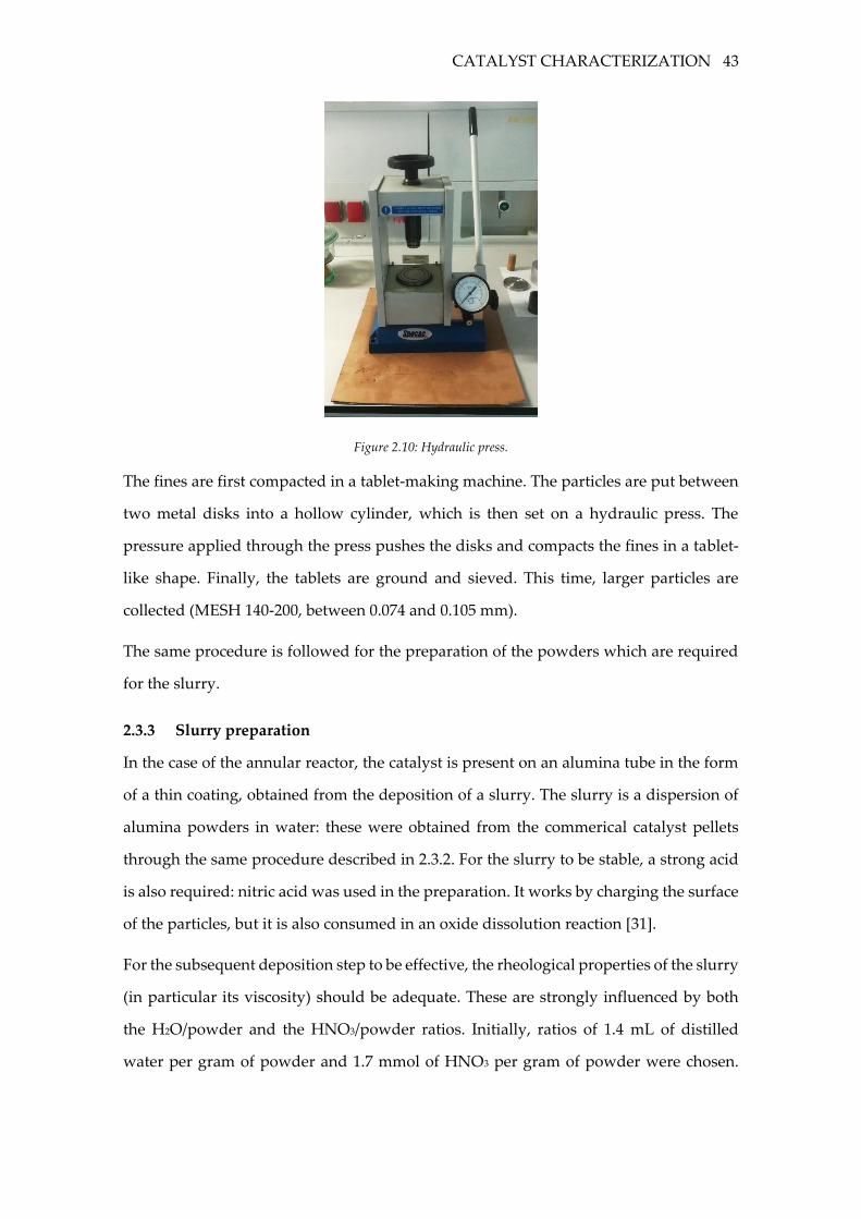
Figure 2.10: Hydraulic press. .................................................................................................. 43
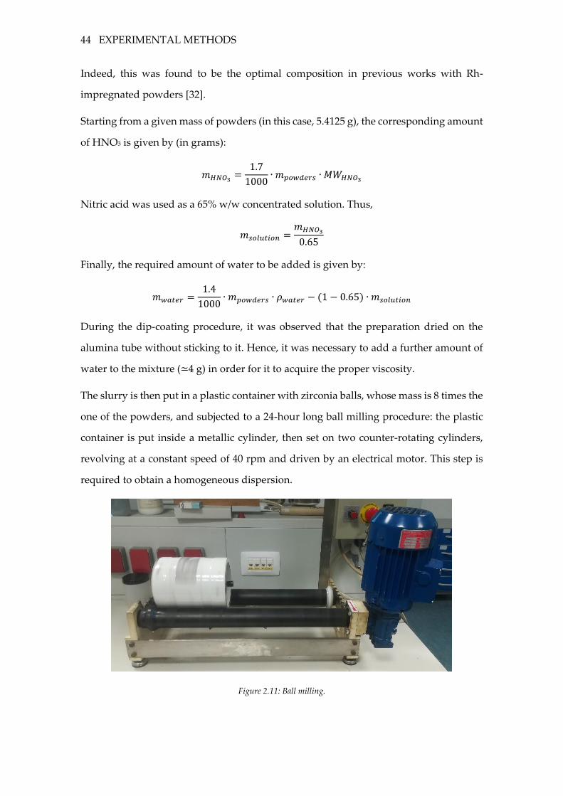
Figure 2.11: Ball milling. .......................................................................................................... 44
Figure 3.1: BED1. ....................................................................................................................... 50
Figure 3.2.: Conversion drift at 60 °C over a 150-minute time period (BED3).
GHSV=160000 NL/h/kg. Inlet composition: 40% H2, 1% CO, 1% O2. ................................ 52
Figure 3.3: Effect of the GHSV in BED1. Inlet composition: 40% H2, 1% CO, 1% O2. ...... 60
Figure 3.4: Conversion drift in BED2. GHSV=240000 NL/h/kg. Inlet composition: 40% H2,
1% CO, 1% O2. Injections from 6 up to 15 were carried out around 30 mins after the first
five ones, at 10-minute intervals. ........................................................................................... 62
Figure 3.5: Effect of the GHSV in BED2. Inlet composition: 40% H2, 1% CO, 1% O2. ...... 63
xii
Figure 3.6: Effect of oxygen concentration in BED2. GHSV=240000 NL/h/kg. ................. 65
Figure 3.7: Check on the presence of interphase and radial temperature gradients in BED2
(GHSV=240000 NL/h/kg, 40% H2, 1% CO, 1% O2). In blue: the term at the left hand side
of each criterion (see 3.2.2 and 3.2.3). In red: the threshold. .............................................. 66
Figure 3.8: Trend of CO conversion for the three reference tests carried out in BED3. Inlet
composition: 40% H2, 1% CO, 1% O2. GHSV=160000 NL/h/kg. ......................................... 67
Figure 3.9: Conversion drift in BED3 (inlet composition: 40% H2, 1% CO, 1% O2.
GHSV=160000 NL/h/kg). ......................................................................................................... 68
Figure 3.10: Comparison among BED1, BED2 and BED3. Left: comparison between BED1
(unconditioned) and BED2 (conditioned in hydrogen) at GHSV=80000 NL/h/kg. Right:
comparison between BED2 and BED3 at GHSV=160000 NL/h/kg. Inlet composition: 40%
H2, 1% CO, 1% O2. .................................................................................................................... 70
Figure 3.11: Check on the presence of interphase and radial temperature gradients in
BED3 (GHSV=160000 NL/h/kg, 40% H2, 1% CO, 1% O2). In blue: the term at the left hand
side of each criterion (see 3.2.2 and 3.2.3). In red: the threshold. ...................................... 70
Figure 4.1: Reference tests performed on V1. Inlet composition: 40% H2, 1% CO, 1% O2.
GHSV=500000 NL/h/kg. .......................................................................................................... 73
Figure 4.2: CO conversion drift at 100 °C, 90 °C and 80 °C on reactor V1. Inlet
composition: 40% H2, 1% CO, 1% O2. GHSV=500000 NL/h/kg. ......................................... 74
Figure 4.3: Trend of the outlet flow rate of CO for the three injections taken at each
temperature. GHSV=500000 NL/h/kg. Inlet concentration: 40% H2, 1% CO, 1% O2. ...... 75
Figure 4.4: Effect of the GHSV in V1. Inlet composition: 40% H2, 1% CO, 1% O2. .......... 77
Figure 4.5: Axial temperature profiles for the tests performed at 300000 and 1500000
NL/h/kg. ..................................................................................................................................... 78
Figure 4.6: Axial temperature difference between the catalytic bed and the oven for the
tests performed at 300000 and 1500000 NL/h/kg. ................................................................ 78
Figure 4.7: Effect of CO concentration on V1. GHSV=500000 NL/h/kg. ........................... 81
Figure 4.8: Effect of oxygen concentration on V1. GHSV=500000 NL/h/kg. .................... 83
Figure 4.9: Effect of the GHSV in the absence of hydrogen on V1 (squares). The results
are compared with the ones of the experiments carried out in the presence of hydrogen
(triangles). Inlet composition: 40% H2, 1% CO, 1% O2. ....................................................... 85
xiii
Figure 4.10: Effect of oxygen concentration on V1 in the absence of hydrogen.
GHSV=500000 NL/h/kg. .......................................................................................................... 87
Figure 4.11: Effect of CO concentration on V1 in the absence of hydrogen. GHSV=500000
NL/h/kg. ..................................................................................................................................... 89
Figure 5.1: Bilogarithmic plot for the data at varying CO concentration for the differential
analysis. ..................................................................................................................................... 97
Figure 5.2: Bilogarithmic plot for the data at varying O2 concentration for the differential
analysis. ..................................................................................................................................... 98
Figure 5.4: Results of the model for the tests in the absence of hydrogen: effect of the
GHSV. ...................................................................................................................................... 102
Figure 5.5: Results of the model for the tests in the absence of hydrogen: effect of CO
concentration. .......................................................................................................................... 102
Figure 5.6: Results of the model for the tests in the absence of hydrogen: effect of O2
concentration. .......................................................................................................................... 102
Figure 5.3: Comparison between the model and Prova 43 (GHSV=500000 NL/h/kg, 1%
CO, 1% O2, no hydrogen). .................................................................................................... 103
Figure 5.7: Trends of yCO2 and yH2O as a function of the percentage of CO, at three
different temperatures. .......................................................................................................... 104
Figure 5.8: Trends of yCO2 and yH2O as a function of the percentage of O2, at three
different temperatures. .......................................................................................................... 106
Figure 5.9: Arrhenius' plot for CO oxidation in the absence of hydrogen. .................... 107
Figure 5.10: Arrhenius' plot for CO oxidation in the presence of hydrogen. ................ 108
Figure 5.11: Arrhenius' plots for CO oxidation in the presence of hydrogen. Left: low
temperatures. Right: high temperatures. ............................................................................ 108
Figure 5.12: Results of the model. Effect of the GHSV. ..................................................... 112
Figure 5.13: Results of the model. Effect of CO concentration. ........................................ 113
Figure 5.14: Results of the model. Effect of O2 concentration. ......................................... 114
xiv
LIST OF TABLES
Table 2.1: Properties of the catalyst pellets. .......................................................................... 41
Table 2.2: Results of BET. ........................................................................................................ 41
Table 2.3: Results of mercury porosimetry. .......................................................................... 41
Table 2.4: Properties of tube V1. ............................................................................................. 45
Table 3.1: Packed bed reactors used in this Thesis work. ................................................... 49
Table 4.1: Tests carried out on V1. ......................................................................................... 73
Table 5.1: Data at varying CO concentration for the differential analysis in the absence
of hydrogen. .............................................................................................................................. 97
Table 5.2: Results of the differential analysis on the reaction order with respect to CO.
..................................................................................................................................................... 97
Table 5.3: Data at varying O2 concentration for the differential analysis in the absence of
hydrogen. ................................................................................................................................... 98
Table 5.4: Results of the differential analysis on the reaction order with respect to O2. 99
Table 5.5: Kinetic parameters for CO oxidation in the absence of hydrogen. ............... 101
Table 5.6: Kinetic parameters for CO oxidation in the presence of hydrogen. .............. 112
Table 5.7: Kinetic parameters for methanation (from [30]). ............................................. 115
Table 5.8: Comparison between the initial rates of methanation and PrOx. ................. 116

xv
1 STATE OF THE ART
1.1 MICROGEN30
1.1.1 Description of the unit
MICROGEN30 is a project funded by the Ministry of Economic Development within the
Industria 2015 program, and led by ICI Caldaie. The project consists in developing and
operating a micro-combined heat and power (micro-CHP) system of small-medium scale
for residential applications, based on PEM (Proton Exchange Membrane) fuel cells. It can
generate 10-30 kW of electric power and 50 kW of thermal power [1].
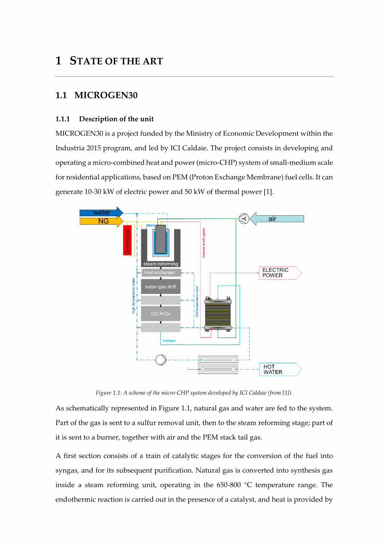
Figure 1.1: A scheme of the micro-CHP system developed by ICI Caldaie (from [1]).
As schematically represented in Figure 1.1, natural gas and water are fed to the system.
Part of the gas is sent to a sulfur removal unit, then to the steam reforming stage; part of
it is sent to a burner, together with air and the PEM stack tail gas.
A first section consists of a train of catalytic stages for the conversion of the fuel into
syngas, and for its subsequent purification. Natural gas is converted into synthesis gas
inside a steam reforming unit, operating in the 650-800 °C temperature range. The
endothermic reaction is carried out in the presence of a catalyst, and heat is provided by
HYDROGEN PRODUCTION 17
means of the burner. Together with steam reforming, water gas shift always takes place
inside the system. Being it an exothermic reaction, at such high temperatures CO is
converted to CO2 only to a limited extent. Since carbon monoxide a poison for the anode
of the PEMFC, it must be removed up to a very small concentration (10 ppm). In order
to do so, a high temperature WGS stage, a low temperature WGS reactor and a final CO
PrOx unit are present.
Electric power is produced by means of four stacks of PEM fuel cells, fed with the
hydrogen exiting the first section and with air. The hot water supply is obtained by
means of water-water heat exchangers: heat is recovered from both the cooling systems
of the fuel cells, and in between the catalytic stages.
In the following sections, a brief description of each of the reactions taking place in the
catalytic stages will be provided, with a summary of the possible solutions which are
available, or under study, for small-scale applications. Particular attention will be given
to the reaction of preferential oxidation of CO.
1.2 HYDROGEN PRODUCTION
1.2.1 Main processes for hydrogen production
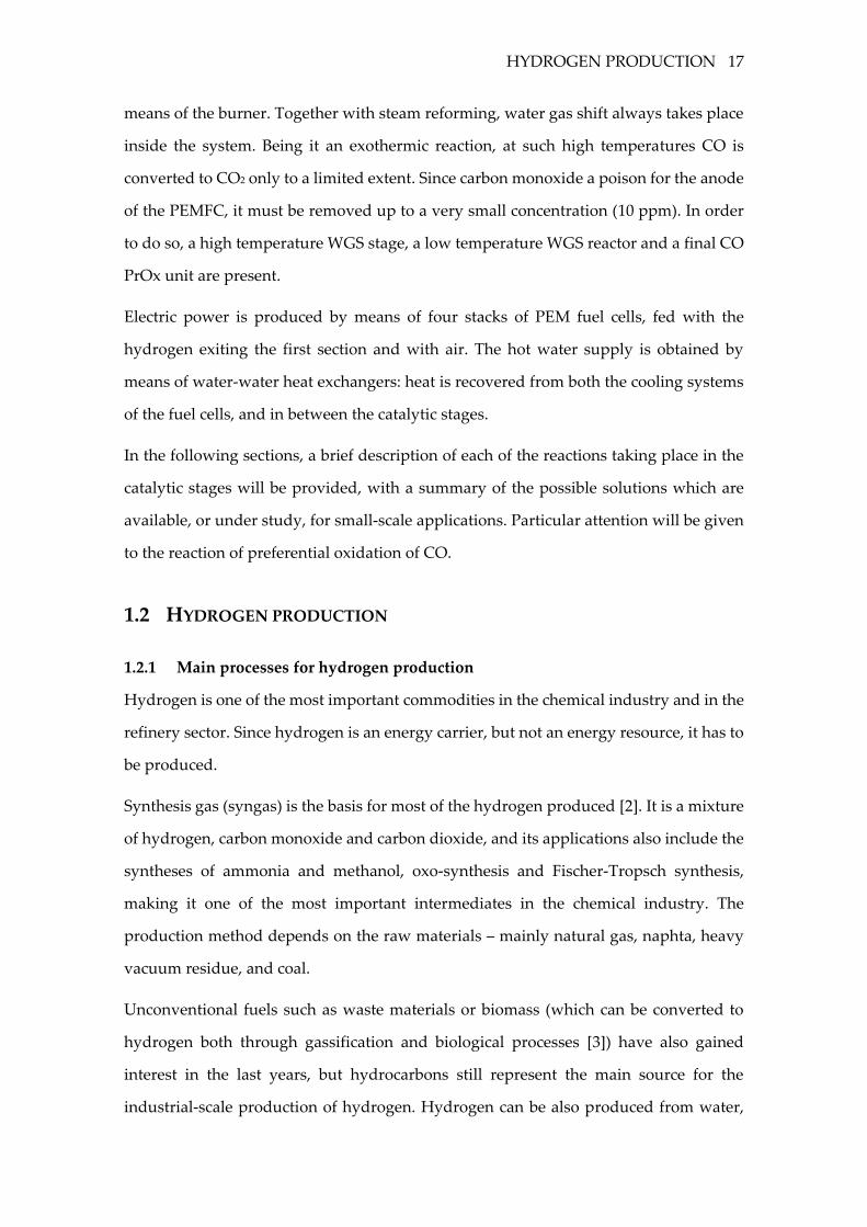
Hydrogen is one of the most important commodities in the chemical industry and in the
refinery sector. Since hydrogen is an energy carrier, but not an energy resource, it has to
be produced.
Synthesis gas (syngas) is the basis for most of the hydrogen produced [2]. It is a mixture
of hydrogen, carbon monoxide and carbon dioxide, and its applications also include the
syntheses of ammonia and methanol, oxo-synthesis and Fischer-Tropsch synthesis,
making it one of the most important intermediates in the chemical industry. The
production method depends on the raw materials – mainly natural gas, naphta, heavy
vacuum residue, and coal.
Unconventional fuels such as waste materials or biomass (which can be converted to
hydrogen both through gassification and biological processes [3]) have also gained
interest in the last years, but hydrocarbons still represent the main source for the
industrial-scale production of hydrogen. Hydrogen can be also produced from water,
18 STATE OF THE ART
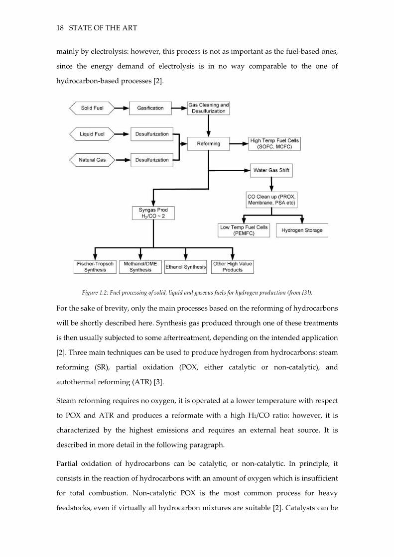
mainly by electrolysis: however, this process is not as important as the fuel-based ones,
since the energy demand of electrolysis is in no way comparable to the one of
hydrocarbon-based processes [2].
Figure 1.2: Fuel processing of solid, liquid and gaseous fuels for hydrogen production (from [3]).
For the sake of brevity, only the main processes based on the reforming of hydrocarbons
will be shortly described here. Synthesis gas produced through one of these treatments
is then usually subjected to some aftertreatment, depending on the intended application
[2]. Three main techniques can be used to produce hydrogen from hydrocarbons: steam
reforming (SR), partial oxidation (POX, either catalytic or non-catalytic), and
autothermal reforming (ATR) [3].
Steam reforming requires no oxygen, it is operated at a lower temperature with respect
to POX and ATR and produces a reformate with a high H2/CO ratio: however, it is
characterized by the highest emissions and requires an external heat source. It is
described in more detail in the following paragraph.
Partial oxidation of hydrocarbons can be catalytic, or non-catalytic. In principle, it
consists in the reaction of hydrocarbons with an amount of oxygen which is insufficient
for total combustion. Non-catalytic POX is the most common process for heavy
feedstocks, even if virtually all hydrocarbon mixtures are suitable [2]. Catalysts can be
HYDROGEN PRODUCTION 19
used to lower the operating temperatures: in the case of natural gas, Ni and Rh-based
catalysts are typically used. Due to the exothermic nature of the oxidation reactions,
temperature is difficult to control [3].
Autothermal reforming is inbetween SR and POX: it adds steam to catalytic partial
oxidation. The heat required by the steam reforming reaction is provided through partial
oxidation, taking place in the thermal part of the reactor. Hence, there is no need for an
external heat source, simplifying the system and making it more flexible. However, the
oxygen to fuel ratio must be carefully controlled at all times, and in most cases an
expensive air separation unit is required.
1.2.2 Steam reforming
Steam reforming involves the reaction of steam with the fuel, in the presence of a
catalyst. The desired reaction is, in the case of methane:
CH4 + H2O ↔ CO + 3 H2
The reaction is strongly endothermic. In addition to steam reforming, the water-gas shift
reaction (slightly exothermic) also takes place in the system, producing some CO2:
CO + H2 ↔ CO2 + H2O
To obtain satisfying yields, the working temperature is around 800 °C. Despite the main
reaction being characterized by an increase in the number of moles, steam reforming is
usually carried out at pressures up to 30 atm, since the downstream processes are usually
performed under pressure. The steam to methane ratio is an important process
parameter, since not only does it influence the outlet composition, but it also prevents
coke formation [2]:
C + H2O ↔ CO + H2
Kinetically speaking, methane reforming can be described as a first-order reaction, no
matter the operating pressure. While at low temperatures the diffusion rate is much
higher than the reaction rate, at high temperatures pore diffusion has a strong impact on
the conversion [2]. Catalysts for steam reforming can be cathegorized into two main
groups: non-precious metals (typically Ni) and precious metals from Group VIII
elements (usually Pt or Rh) [3], very often promoted with alkali which are known for
increasing the activity of the catalyst and to facilitate coke gassification [4]. Due to severe
20 STATE OF THE ART
heat and mass transfer limitiations, the effectiveness factor for the catalyst in
conventional steam reformers is usually very low: thus, since rarely is the activity of the
catalyst a limiting factor, less expensive Ni-based catalysts are usually preferred [3]. The
catalyst is usually in the form of thick-walled, 16-mm diameter Raschig rings [2]. Other
common shapes include spoked wheels, gear wheels, or rings with several holes, and
are advantageous because of the low associated pressure drop. The catalyst can be
precipitated (higher activity, more prone to sintering) or impregnated (preferred due to
their higher mechanical resistance). Common supports include α-Al2O3 and MgO. Sulfur
is a strong poison for the catalyst and must be removed from the feed: this is usually
done by means of a zinc oxide desulfurization system.
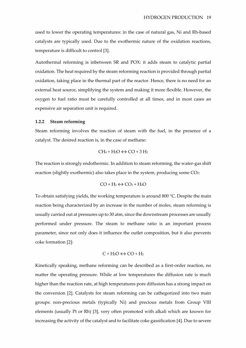
The reaction is carried out industrially inside tubular reactors, built using special alloys.
Tubes are heated from the outside in fire-box-type units, both wall-fired and top- or
bottom-fired: burner geometry, flame length and the distance from the flame to the
reformer are all parameters that influence the homogeneity of heat transfer. Natural gas,
or low-sulfur containing hydrocarbons are employed as fuel.
Figure 1.3: Examples of reformers. A: top-fired reformers. B: wall-fired reformers (from [2]).
1.2.3 Steam reforming in micro-CHPs
The ideal fuel for a PEM fuel cell would be pure hydrogen. However, cost and technical
constraints make it difficult to store hydrogen in the necessary amount. Hence, hydrogen
gas is usually generated on site and on demand. Typical feedstocks are natural gas,
gasoline, LPG, and methanol [4].
WATER GAS SHIFT 21
Low-temperature PEM fuel cells usually exploit hydrogen produced by external
reforming with steam, air, or both. Depending on the operating conditions, an outlet
stream containing 3-10% CO is obtained. The main features of a catalyst for steam
reforming in fuel cell applications include high activity towards the fuel of choice,
resistance to poisoning, reduced start-up times, mechanical resistance and stability at
high temperatures under both steady-state and transient conditions. The support is
usually in the form of a ceramic or metallic monolith, foam, or some other structured
inert.
Frequently used catalysts for methane steam reforming include Rh, Pt and Ru [5]: the
advantage of precious metal catalysts is their high activity, durability, and low tendency
to both coking and sulfur poisoning.
The steam reforming unit of the MICROGEN30 fuel processor is characterized by three
main features [1]: the use of a precious metal catalyst; an annular reactor, packed with
catalyst particles diluted with highly conductive SiC beads, being heat transfer crucial
for this process [5]; a proprietary design of the burner, developed by ICI Caldaie.
1.3 WATER GAS SHIFT
For the majority of industrial processes, the carbon monoxide content in syngas as it is
produced from steam reforming is higher than required [2]. The water gas shift reaction
is typically exploited to remove this undesired amount of carbon monoxide, and the
same reaction is carried out in fuel processors.
Water gas shift is a catalytic reaction which converts CO and water into CO2 and
hydrogen:
CO + H2O ↔ CO2 + H2
The reaction is equimolar, thus the equilibrium conversion does not depend on the
operating pressure. On the contrary, the equilibrium composition does depend on the
temperature: since the reaction is slightly exothermic, the operating temperature should
be as low as possible, compatibly with the activity of the catalyst. The usual temperature
ranges are 300-510 °C for the high-temperature shift (HTS), and 180-270 °C for the low-
temperature shift (LTS). The upper temperature limit for HTS is dictated by the
22 STATE OF THE ART
resistance of the catalyst to sintering, while the lower limit for LTS is dictated both by
the poor activity of the catalyst and by the need of preventing water condensation and
the subsequent damage to the catalyst. The reaction is carried out industrially inside
multi-stage adiabatic reactors with inter-stage cooling. The two catalytic systems are set
in a series configuration: first the HTS and then, after an intermediate cooling, the LTS,
which is necessary to reduce the amount of CO from 2% to <0.5% [5].
Catalysts for HTS are usually Fe-Cr2O3-based, with Cu very often used as a promoter [2].
They are supplied in the oxidized condition, and reduced in situ. More recently, both Al
and Ce have been proposed as substitutes for Cr, which is active and stable, but also
highly toxic and thus leads to high disposal costs [6]. HTS catalysts have a lower activity
with respect to LTS catalysts, but they are quite resistant to impurities. Rapid
temperature and pressure changes must be avoided, since they lead to the disintegration
of the structure [2]. Catalysts for LTS include Cu-ZnO-Al2O3, where Cu represents the
active species. These catalysts were developed in more recent times, and have the
advantage of being active at lower temperatures. They are very sensitive to sulfur
poisoning: hence, a ZnO guard bed is present upstream of the LTS reactor. Moreover,
the reduced Cu species is pyrophoric [5] and the discharge process must be carried out
very carefully. Other categories of catalysts include ceria and noble-metal based
catalysts, carbon based catalysts and nanostructured catalysts [6].
Since the activity of the LTS is not too high at such low temperatures, typical space
velocities are about 1500-2000 h-1 [5]. Both LTS and HTS catalysts are characterized by
large volumes and hence large heat capacities, leading to a very slow response in
transient operations – an important limit for fuel cell-integrated fuel processors. Water
condensation, which is possible in the case of sudden stops, is also detrimental for the
catalyst. For these reasons, conventional base metal catalysts are not indicated for water
gas shift in fuel processing systems.
Water gas shift catalysts for fuel processing applications include Pt. Pt-containing
catalysts can be used at high temperatures, are highly effective (especially if used on a
monolith support) and show a zero-order kinetics with respect to CO, leading to a good
performance independently of the inlet concentration of CO. However, these catalysts
should be carefully designed to avoid the strongly exothermic methanation reaction.
PREFERENTIAL OXIDATION OF CO 23
Gold-containing catalysts have also been developed. No other precious metal has shown
promising activity towards WGS [5].
1.4 PREFERENTIAL OXIDATION OF CO
1.4.1 Introduction
Water gas shift allows achieving an outlet composition with a typical CO content of 0.5-
2% v/v [7]. CO is known to strongly adsorb on the Pt anode of the PEM fuel cell,
hindering the electro-catalytic oxidation of hydrogen [5] and causing irreversible
damage [7]. A way to partially recover the cell potential drop associated to the presence
of CO is the so-called air bleed [5], i.e. the addition of air to the reformate and the
subsequent oxidation of some of the chemisorbed CO. However, this technique has a
negative impact on the fuel cell operation, since it leads to the consumption of some of
the fuel, and to the dilution of the reformate. Therefore, the residual CO should be
removed upstream of the fuel cell as thoroughly as possible: concentrations of <10 ppmv
are to be reached.
Different processes have been developed for the removal of this residual amount of CO,
among them the pressure swing adsorption (PSA), and the employement of selective
hydrogen membranes: both methods require sufficiently high pressures to be effective
[5]. Among the catalytic methods for CO abatement, methanation and preferential
oxidation are the most widespread. Due to the large availability of highly selective
catalysts, efficient process control, lower operation costs and relatively simple
implementation [7], preferential oxidation is vastly employed in fuel cell applications.
Industrial applications of CO PrOx in hydrogen-rich streams date back as far as the early
1960s [5], when Engelhard developed a highly active and selective Pt-based catalyst,
named Selectoxo™, and a process for the selective oxidation of carbon monoxide in
ammonia synthesis gas. In particular, this process could be used for the treatment of gas
streams containing from a few parts per million up to 3% v/v of carbon monoxide, using
air in a range of about 3:1 to 0.25:1 oxygen to CO ratio, and an optimum GHSV around
5000 cubic feet per hour per cubic foot of catalyst [8].
24 STATE OF THE ART
Catalysts for CO PrOx are well-developed at the industrial scale: however, small-scale
fuel processors are associated to a number of constraints which lead to the development
of new catalysts [9].
A catalyst for preferential oxidation in fuel cell systems should satisfy the following
requirements [5]:
• lowering CO concentration down to <10 ppmv;
• showing high selectivity towards CO oxidation with respect to hydrogen
oxidation. Low selectivity is not only associated to an unnecessary consumption
of hydrogen to form water, but also to over-dilution of the reformate with
nitrogen as a result of excessive air injection;
• avoiding undesired side reactions. Due to the presence of large amounts of
hydrogen and CO2, the reverse water gas shift reaction (rWGS)
CO2 + H2 → CO + H2O
might occur, leading to CO production, especially at low space velocities and as
CO concentration approaches zero [10]. Being it an endothermic reaction, it is
favoured as the temperature increases. CO2 methanation
CO2 + 4 H2 → CH4 + 2 H2O
should also be prevented, since it leads to a large fuel consumption and to
runaway temperature excursions. It is especially favoured on Ru catalysts at
temperatures approaching 200 °C;
• operating within the range of temperatures and GHSVs of the fuel processor.
Thus, the inlet temperature should be compatible with the outlet one of the WGS
stage, or also conveniently to the one at which the fuel cell is operated (around
80-100 °C). At the same time, CO and hydrogen oxidation are highly exothermic
reactions: the heat released in the process can be recovered. The catalyst should
also show adequate activity within a wide range of space velocities, especially at
maximum flow.
• showing good chemical and mechanical resistance to the temperature cycling, air
exposure and water condensation associated to start-up and shut-down
procedures [9]. The catalyst must be stable even after thousands of start and stop
operations.
PREFERENTIAL OXIDATION OF CO 25
1.4.2 Catalysts reported in the literature
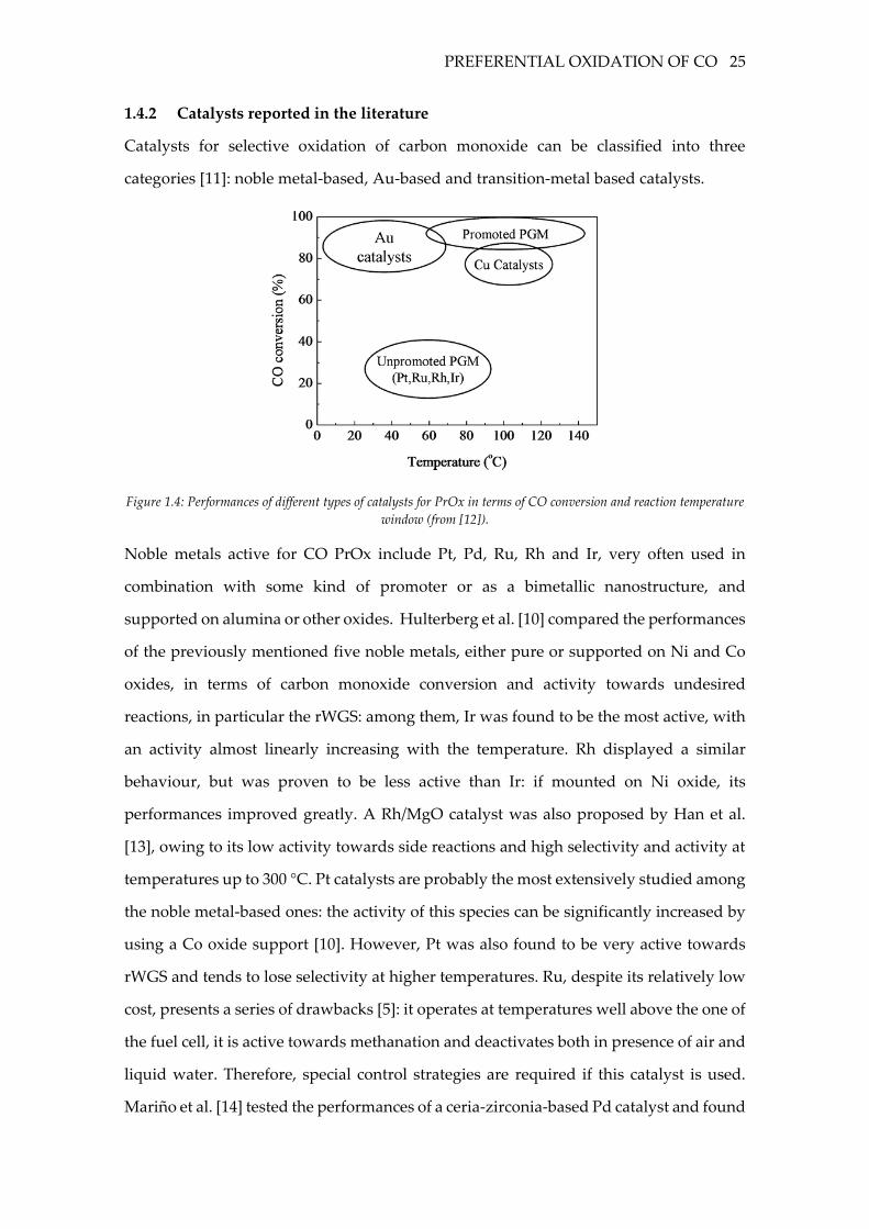
Catalysts for selective oxidation of carbon monoxide can be classified into three
categories [11]: noble metal-based, Au-based and transition-metal based catalysts.
Figure 1.4: Performances of different types of catalysts for PrOx in terms of CO conversion and reaction temperature
window (from [12]).
Noble metals active for CO PrOx include Pt, Pd, Ru, Rh and Ir, very often used in
combination with some kind of promoter or as a bimetallic nanostructure, and
supported on alumina or other oxides. Hulterberg et al. [10] compared the performances
of the previously mentioned five noble metals, either pure or supported on Ni and Co
oxides, in terms of carbon monoxide conversion and activity towards undesired
reactions, in particular the rWGS: among them, Ir was found to be the most active, with
an activity almost linearly increasing with the temperature. Rh displayed a similar
behaviour, but was proven to be less active than Ir: if mounted on Ni oxide, its
performances improved greatly. A Rh/MgO catalyst was also proposed by Han et al.
[13], owing to its low activity towards side reactions and high selectivity and activity at
temperatures up to 300 °C. Pt catalysts are probably the most extensively studied among
the noble metal-based ones: the activity of this species can be significantly increased by
using a Co oxide support [10]. However, Pt was also found to be very active towards
rWGS and tends to lose selectivity at higher temperatures. Ru, despite its relatively low
cost, presents a series of drawbacks [5]: it operates at temperatures well above the one of
the fuel cell, it is active towards methanation and deactivates both in presence of air and
liquid water. Therefore, special control strategies are required if this catalyst is used.
Mariño et al. [14] tested the performances of a ceria-zirconia-based Pd catalyst and found
26 STATE OF THE ART
it to have a very poor activity and selectivity towards CO oxidation if compared to the
corresponding Pt and Ir catalysts, possibly due to its oxidation to PdO.
The main drawback of PGMs is the poor activity in the low temperature range, since the
surface is predominantly covered with CO, hindering O2 adsorption [12]. Reducible
oxides active for oxygen storage, such as CeO2, have been proven to have a significant
impact on the performance of noble-metal based catalysts [14]. In general, reducible
oxides have the advantage of weakening CO adsorption while also providing additional
sites for oxygen adsorption or activation, turning the competitive Langmuir-
Hinshelwood mechanism between CO and oxygen for active sites into a non-competitive
one [15], [12]. Among reducible oxides, iron oxide has shown remarkable performances
[16], [17]. The performances of PGMs can be also improved by means of alkali metal
cations, such as Cs and Rb: if the low selectivity is assumed to be related to a spillover-
mediated hydrogen oxidation reaction, the enhancing effect of alkali can be explained
by the fact that these species are capable of supporting the hydroxyl groups required for
this unselective path [18].
Au-based catalysts have the advantage of showing good performance at lower
temperatures (around 100 °C) with respect to other noble metals, thus allowing a
straightforward implementation of the PrOx reactor in the same cooling circuit as the
PEM fuel cell, working at around 80 °C [19]. Despite being a poor catalyst in the pure
form due to the weak interaction with adsorbates, Au possesses high activity if highly
dispersed on a metal oxide support [14].
CuO-CeO2 are considered an economical alternative to noble-based metal catatalysts
[20]: these catalysts have been found to have good catalytic activity and selectivity.
Avgouropoulos et al. [21] compared the performances of Pt/γ-Al2O3, Au/α-Fe2O3 and
CuO–CeO2 catalysts and concluded that, while the Au-based catalyst is the most active
(capable of achieving 100% conversion at 45 °C for high enough contact times) and the
better one in the low temperature range, the CuO–CeO2 is the most selective and
preferable at higher temperatures; however, Pt/γ-Al2O3 is the most resistant towards CO2
deactivation, its performances in terms of CO oxidation being more or less unaffected
by CO2 partial pressure.
PREFERENTIAL OXIDATION OF CO 27
1.4.3 Mechanism of CO preferential oxidation on PGMs
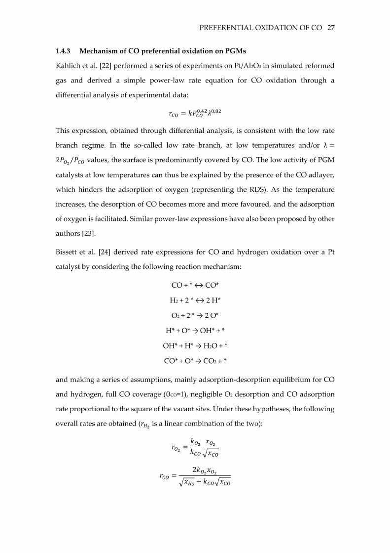
Kahlich et al. [22] performed a series of experiments on Pt/Al2O3 in simulated reformed
gas and derived a simple power-law rate equation for CO oxidation through a
differential analysis of experimental data:
𝑟𝐶𝑂 = 𝑘𝑃𝐶𝑂0.42𝜆0.82
This expression, obtained through differential analysis, is consistent with the low rate
branch regime. In the so-called low rate branch, at low temperatures and/or λ =
2𝑃𝑂2 𝑃𝐶𝑂⁄ values, the surface is predominantly covered by CO. The low activity of PGM
catalysts at low temperatures can thus be explained by the presence of the CO adlayer,
which hinders the adsorption of oxygen (representing the RDS). As the temperature
increases, the desorption of CO becomes more and more favoured, and the adsorption
of oxygen is facilitated. Similar power-law expressions have also been proposed by other
authors [23].
Bissett et al. [24] derived rate expressions for CO and hydrogen oxidation over a Pt
catalyst by considering the following reaction mechanism:
CO + * ↔ CO*
H2 + 2 * ↔ 2 H*
O2 + 2 * → 2 O*
H* + O* → OH* + *
OH* + H* → H2O + *
CO* + O* → CO2 + *
and making a series of assumptions, mainly adsorption-desorption equilibrium for CO
and hydrogen, full CO coverage (θCO=1), negligible O2 desorption and CO adsorption
rate proportional to the square of the vacant sites. Under these hypotheses, the following
overall rates are obtained (𝑟𝐻2 is a linear combination of the two):
𝑟𝑂2 =𝑘𝑂2𝑘𝐶𝑂
𝑥𝑂2
√𝑥𝐶𝑂
𝑟𝐶𝑂 =2𝑘𝑂2𝑥𝑂2
√𝑥𝐻2 + 𝑘𝐶𝑂√𝑥𝐶𝑂
28 STATE OF THE ART
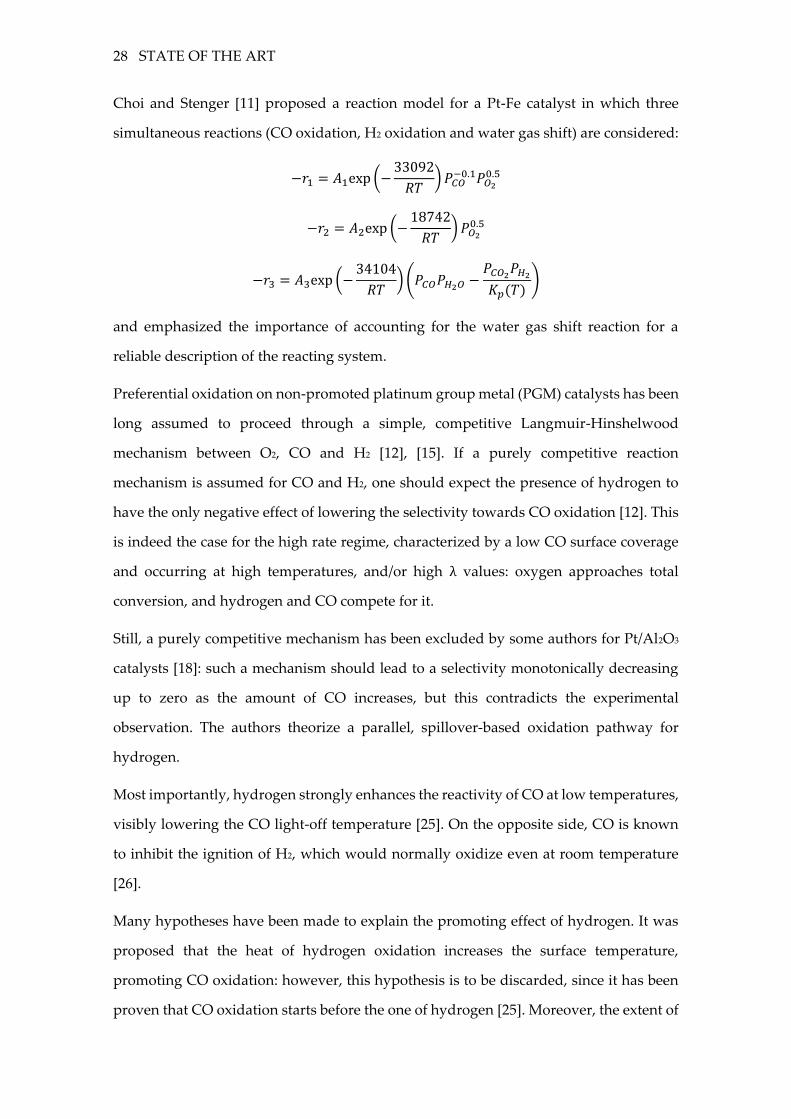
Choi and Stenger [11] proposed a reaction model for a Pt-Fe catalyst in which three
simultaneous reactions (CO oxidation, H2 oxidation and water gas shift) are considered:
−𝑟1 = 𝐴1exp(−33092
𝑅𝑇)𝑃𝐶𝑂
−0.1𝑃𝑂20.5
−𝑟2 = 𝐴2exp(−18742
𝑅𝑇)𝑃𝑂2
0.5
−𝑟3 = 𝐴3exp(−34104
𝑅𝑇)(𝑃𝐶𝑂𝑃𝐻2𝑂 −
𝑃𝐶𝑂2𝑃𝐻2𝐾𝑝(𝑇)
)
and emphasized the importance of accounting for the water gas shift reaction for a
reliable description of the reacting system.
Preferential oxidation on non-promoted platinum group metal (PGM) catalysts has been
long assumed to proceed through a simple, competitive Langmuir-Hinshelwood
mechanism between O2, CO and H2 [12], [15]. If a purely competitive reaction
mechanism is assumed for CO and H2, one should expect the presence of hydrogen to
have the only negative effect of lowering the selectivity towards CO oxidation [12]. This
is indeed the case for the high rate regime, characterized by a low CO surface coverage
and occurring at high temperatures, and/or high λ values: oxygen approaches total
conversion, and hydrogen and CO compete for it.
Still, a purely competitive mechanism has been excluded by some authors for Pt/Al2O3
catalysts [18]: such a mechanism should lead to a selectivity monotonically decreasing
up to zero as the amount of CO increases, but this contradicts the experimental
observation. The authors theorize a parallel, spillover-based oxidation pathway for
hydrogen.
Most importantly, hydrogen strongly enhances the reactivity of CO at low temperatures,
visibly lowering the CO light-off temperature [25]. On the opposite side, CO is known
to inhibit the ignition of H2, which would normally oxidize even at room temperature
[26].
Many hypotheses have been made to explain the promoting effect of hydrogen. It was
proposed that the heat of hydrogen oxidation increases the surface temperature,
promoting CO oxidation: however, this hypothesis is to be discarded, since it has been
proven that CO oxidation starts before the one of hydrogen [25]. Moreover, the extent of
PREFERENTIAL OXIDATION OF CO 29
the decrease in the light-off temperature related to the exotherm only is too limited, and
in any case not proportional to the concentration of hydrogen [27]. The simple
competition for active sites between hydrogen and CO and the related thermal effects
alone seem unable to describe the enhancement in the reactivity of CO.
Some authors [27] theorized a hydrogen-related reduction in the adsorption heat of CO:
this is in contradiction with other works proving no significant decrease in the surface
coverage of CO in the presence of hydrogen [28]. Other authors [22] theorized the
formation of formate species (consuming Pt-bonded CO) on the alumina support to
explain the increase in the reaction rate.
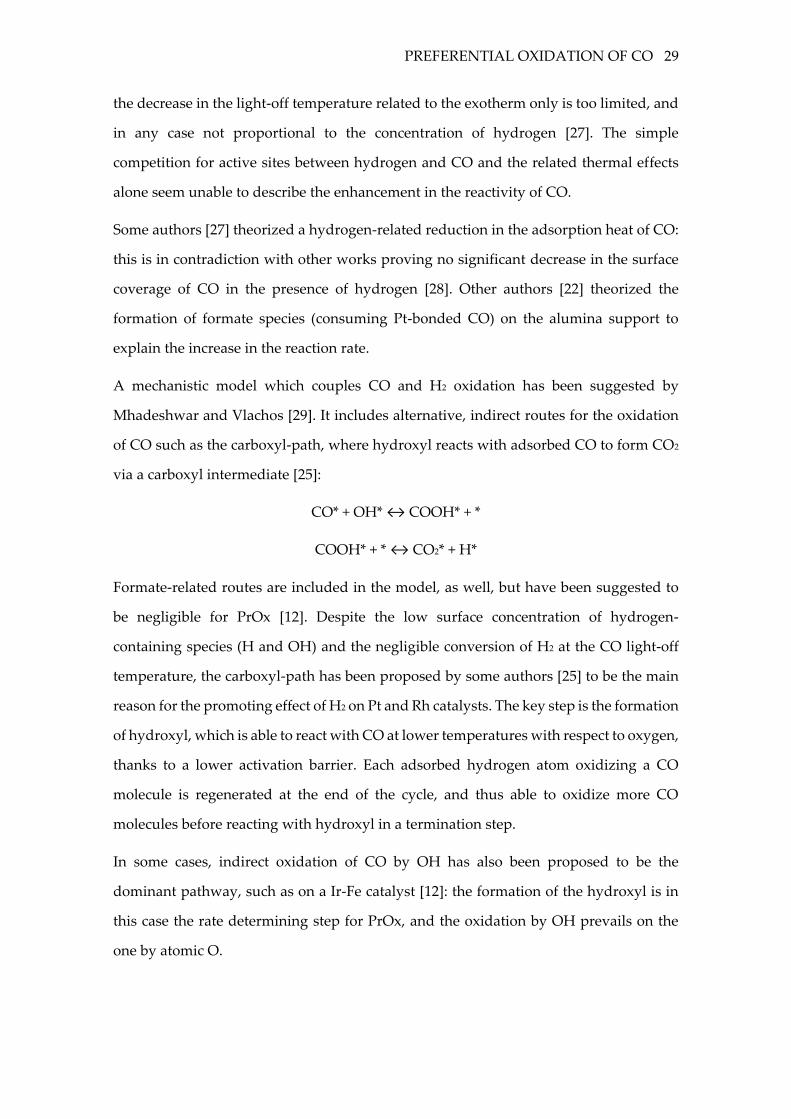
A mechanistic model which couples CO and H2 oxidation has been suggested by
Mhadeshwar and Vlachos [29]. It includes alternative, indirect routes for the oxidation
of CO such as the carboxyl-path, where hydroxyl reacts with adsorbed CO to form CO2
via a carboxyl intermediate [25]:
CO* + OH* ↔ COOH* + *
COOH* + * ↔ CO2* + H*
Formate-related routes are included in the model, as well, but have been suggested to
be negligible for PrOx [12]. Despite the low surface concentration of hydrogen-
containing species (H and OH) and the negligible conversion of H2 at the CO light-off
temperature, the carboxyl-path has been proposed by some authors [25] to be the main
reason for the promoting effect of H2 on Pt and Rh catalysts. The key step is the formation
of hydroxyl, which is able to react with CO at lower temperatures with respect to oxygen,
thanks to a lower activation barrier. Each adsorbed hydrogen atom oxidizing a CO
molecule is regenerated at the end of the cycle, and thus able to oxidize more CO
molecules before reacting with hydroxyl in a termination step.
In some cases, indirect oxidation of CO by OH has also been proposed to be the
dominant pathway, such as on a Ir-Fe catalyst [12]: the formation of the hydroxyl is in
this case the rate determining step for PrOx, and the oxidation by OH prevails on the
one by atomic O.
2 EXPERIMENTAL METHODS
2.1 DESCRIPTION OF THE RIGS
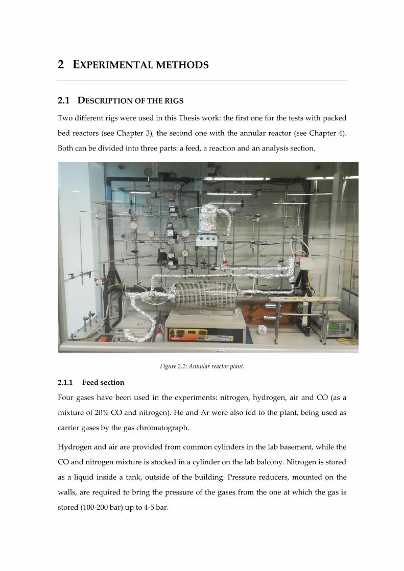
Two different rigs were used in this Thesis work: the first one for the tests with packed
bed reactors (see Chapter 3), the second one with the annular reactor (see Chapter 4).
Both can be divided into three parts: a feed, a reaction and an analysis section.
Figure 2.1: Annular reactor plant.
2.1.1 Feed section
Four gases have been used in the experiments: nitrogen, hydrogen, air and CO (as a
mixture of 20% CO and nitrogen). He and Ar were also fed to the plant, being used as
carrier gases by the gas chromatograph.
Hydrogen and air are provided from common cylinders in the lab basement, while the
CO and nitrogen mixture is stocked in a cylinder on the lab balcony. Nitrogen is stored
as a liquid inside a tank, outside of the building. Pressure reducers, mounted on the
walls, are required to bring the pressure of the gases from the one at which the gas is
stored (100-200 bar) up to 4-5 bar.
DESCRIPTION OF THE RIGS 31
The reactants are fed through four lines, each one equipped with shutoff valves, a mass
flow controller (MFC) and two manometers, one upstream and one downstream of the
mass flow controller. Filters are also present in order to remove any impurity entrained
in the gases.
In the case of the first rig, the following MFCs were employed:
• a 200 NmL/min MFC for the nitrogen line;
• a 700 NmL/min MFC for the hydrogen line;
• a 200 NmL/min MFC for the air line;
• a 50 NmL/min MFC for the CO line.
while in the case of the second rig, those were the MFCs of choice:
• a 700 NmL/min MFC for the nitrogen line;
• a 3 NL/min MFC for the hydrogen line;
• a 100 NmL/min MFC for the air line;
• a 50 NmL/min MFC for the CO line.
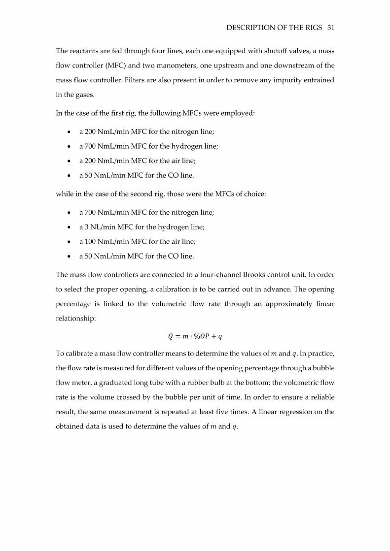
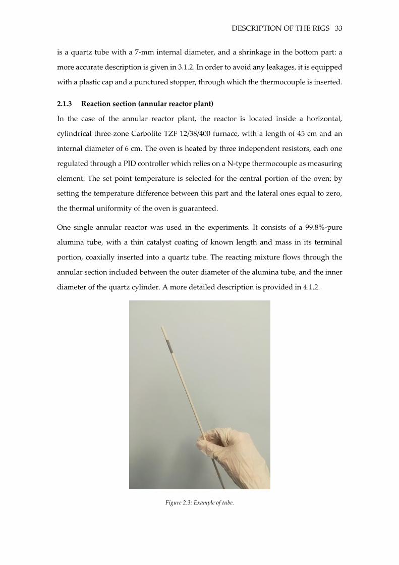
The mass flow controllers are connected to a four-channel Brooks control unit. In order
to select the proper opening, a calibration is to be carried out in advance. The opening
percentage is linked to the volumetric flow rate through an approximately linear
relationship:
𝑄 = 𝑚 ∙ %𝑂𝑃 + 𝑞
To calibrate a mass flow controller means to determine the values of 𝑚 and 𝑞. In practice,
the flow rate is measured for different values of the opening percentage through a bubble
flow meter, a graduated long tube with a rubber bulb at the bottom: the volumetric flow
rate is the volume crossed by the bubble per unit of time. In order to ensure a reliable
result, the same measurement is repeated at least five times. A linear regression on the
obtained data is used to determine the values of 𝑚 and 𝑞.
32 EXPERIMENTAL METHODS
Figure 2.2: Example of calibration curve.
The temperature of the lines is regulated through heating tapes containing electrical
resistances, and set to 120 °C through a TIC. This is required to avoid water condensation
inside the lines. Aluminum sheets are wrapped around the lines to guarantee the
minimization of thermal dispersions. The temperature measurement is carried out
through thermocouples, put in direct contact with the lines.
2.1.2 Reaction section (FBR plant)
The reactants coming from the different lines converge into one single line. The gaseous
mixture is then split into two streams – one sent to the bypass line, the other one to the
reactor. The bypass line is used whenever the reactants are to be sent to the analysis
section without going through the reactor. Both lines are equipped with an upstream
shut-off valve: in the case of the reactor line, a downstream valve is also present to avoid
any reactant backflow. The streams coming from the two lines then mix again
downstream of the reactor.
With regard to the FBR plant, the reaction section includes the reactor, connected to the
heated lines through junctions and whose temperature is regulated through a vertical
Carbolite oven, with a height of 18 cm and an internal diameter of 12.5 mm. The bed
temperature is aquired through a K-type thermocouple, whose hot junction is located at
half of the bed height.
Three different fixed bed reactors were used during the experiments: however, they
were all very similar, differing only for the amount of catalyst and diluent. The reactor
y = 31,518x + 5,0593R² = 0,9999
0.000
0.050
0.100
0.150
0.200
0.250
0.300
0.350
0.400
0 2 4 6 8 10 12
Flo
w r
ate
[Nm
L/m
in]
Opening [%]
DESCRIPTION OF THE RIGS 33
is a quartz tube with a 7-mm internal diameter, and a shrinkage in the bottom part: a
more accurate description is given in 3.1.2. In order to avoid any leakages, it is equipped
with a plastic cap and a punctured stopper, through which the thermocouple is inserted.
2.1.3 Reaction section (annular reactor plant)
In the case of the annular reactor plant, the reactor is located inside a horizontal,
cylindrical three-zone Carbolite TZF 12/38/400 furnace, with a length of 45 cm and an
internal diameter of 6 cm. The oven is heated by three independent resistors, each one
regulated through a PID controller which relies on a N-type thermocouple as measuring
element. The set point temperature is selected for the central portion of the oven: by
setting the temperature difference between this part and the lateral ones equal to zero,
the thermal uniformity of the oven is guaranteed.
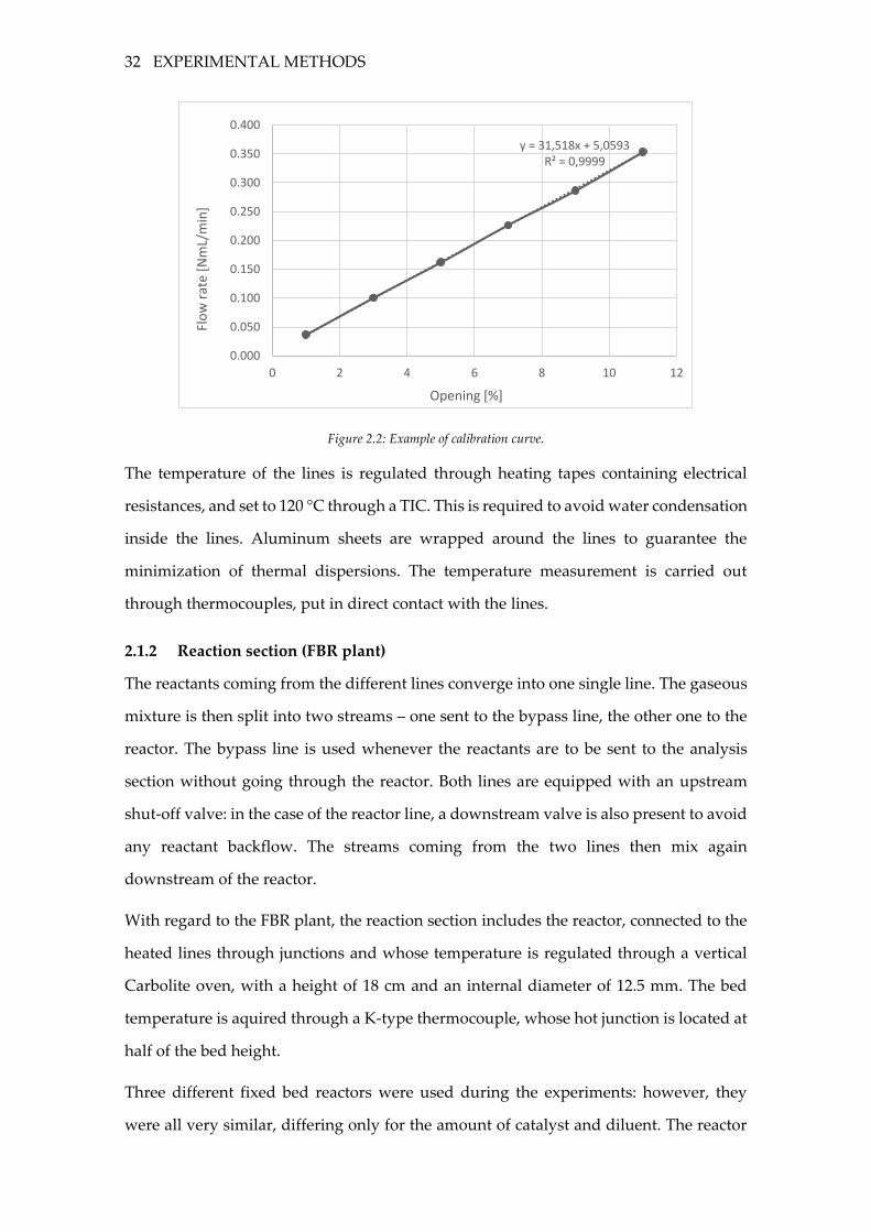
One single annular reactor was used in the experiments. It consists of a 99.8%-pure
alumina tube, with a thin catalyst coating of known length and mass in its terminal
portion, coaxially inserted into a quartz tube. The reacting mixture flows through the
annular section included between the outer diameter of the alumina tube, and the inner
diameter of the quartz cylinder. A more detailed description is provided in 4.1.2.
Figure 2.3: Example of tube.
34 EXPERIMENTAL METHODS
Two K-type thermocouples are also inserted into both the oven and the alumina tube.
By making them slide, it is possible to derive the axial temperature profiles along the
oven and the bed.
2.1.4 Analysis section
A gas chromatographer is required to detect the species exiting the reaction section and
their corresponding concentrations. The operating principle of such instrument is the
different affinity of the gaseous species with a stationary phase.
The gaseous mixture exiting the reactor is injected into the instrument together with an
inert gas, called carrier, and enters a long and thin glass capillary known as column. The
gas chromatographer is equipped with two different columns, each one characerized by
its own stationary phase and carrier gas, and capable of detecting different species. More
in particular:
• one column is equipped with molecular sieves and uses Ar as carrier. The
detected species are H2, O2, N2, CH4 and CO.
• the other column (Plot Q) uses He as carrier and is used to detect air+CO, CO2
and H2O.
The carrier gases are fed to the gas chromatographer at a given pressure and at any time.
The device is hardly ever switched off. When it is not being used, two different methods
can be selected:
• Spegnimento: the TCD is switched off, while the columns and the injector are set
to a temperature close to the ambient one;
• Condizionamento: the TCD is switched off, while the columns and the injector are
heated up to the maximum allowable temperature in order to remove any
undesired compound.
Each species leaves the columns at a different time, called retention time, which depends
on its affinity with the stationary phase, but also on the temperature at which the column
is operated. The time which is required for the analysis is chosen depending on the
largest retention time among the ones of the different species.
A TCD (thermal conductivity detector) is used to detect the components of the gaseous
mixture, separated by the chromatograph. The operating principle is the same as the one
DESCRIPTION OF THE RIGS 35
of the Wheatstone bridge, a device containing four resistors subjected to a constant
thermal flux. Two branches of the bridge are brushed by the carrier gases, while the other
two are swept by the gaseous flow leaving the column. As a component other than the
carrier gas comes in contact with the resistor, its temperature changes due to the different
conductivity of the gaseous flow. This leads to a variation of the resistance and to a so-
called imbalance of the bridge. Such imbalance generates an electrical signal, which
allows the identification of any compound leaving the column. The non-ideality of the
gas mixture might influence the quality of the results.
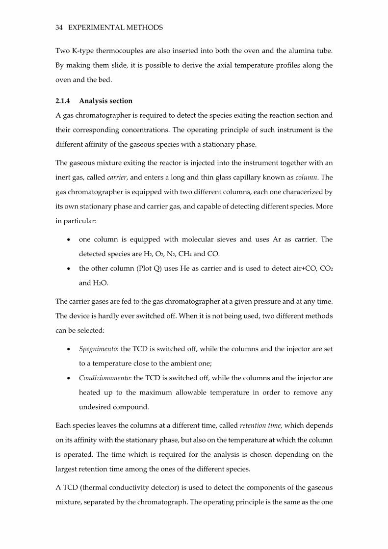
One chromatogram is obtained for each column: such graph depicts the potential
difference generated by the TCD as a function of the time. Each peak corresponds to a
different detected species, which can be identified by its retention time. The area under
the peak is proportional to its concentration: however, the proportionality factor
depends on the species.
Figure 2.4: Example of a chromatogram obtained for column A. From left to right: H2, O2, N2, CO.
In order to convert the areas into concentrations, a calibration is to be carried out.
Calibrating the GC means to calculate the so-called response factors, referred to a species
whose inlet and outlet flow rates are known (usually nitrogen).
The response factor of the i-th species 𝛼𝑖 is defined as:
𝛼𝑖 =
𝑄𝑖𝑄𝑁2𝐴𝑖𝐴𝑁2
36 EXPERIMENTAL METHODS
where 𝑄𝑖 is the flow rate of the i-th species and 𝐴𝑖 the area of the corresponding peak.
Thus, by definition, 𝛼𝑁2 is equal to 1.
In practice, a mixture of nitrogen and of the species under interest is sent to the gas
chromatographer. The flow rates of the two species are associated to a certain opening
percentage of the mass flow controller, and are assumed as known. Once the area of the
two peaks is known, the response factor of the species can be easily computed. It should
be noted that the response factor might vary depending on the fluxes.
Once the response factors have been determined, the volumetric flux of the i-th species
can be calculated starting from the one of nitrogen.
2.2 EXPERIMENTAL PROCEDURES
2.2.1 Start-up of the rig
The suction hood must be working as the experiment is started, in order to avoid any
gas leakage to the working environment. For safety, the room was also equipped with a
CO sensor. First of all, the cylinder containing the CO and nitrogen mixture on the lab
balcony is opened, and so are the valves upstream and downstream of the pressure
reducers on the walls. Shut-off valves are also opened at the entrance of the system.
Before proceeding, it is important to check for any leakages inside the reactor. In order
to do so, the valve upstream of the reactor is kept open, while the one downstream of
the reactor and the one on the bypass line are kept closed. Nitrogen is fed to the reactor
at a certain flow rate: once the pressure indicated by the manometers downstream of the
MFCs has reached a value close to 1 bar, the nitrogen feed is stopped. If no pressure drop
is observed for a sufficiently long amount of time (10-15 s), one can assume no leakage
is present and the experiment can start. After this check, the reactor is to be isolated
through the two shut-off valves. Only the bypass line is left open.
The electrical resistances heating the lines, the temperature controllers and the oven are
then switched on: the temperature of the oven is set to the desired set point. The TCDs
are also turned on, by choosing the proper analysis method for the gas chromatograph
(usually left on Spegnimento after each experiment).
EXPERIMENTAL PROCEDURES 37
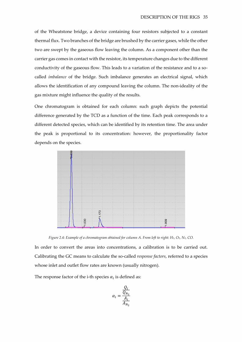
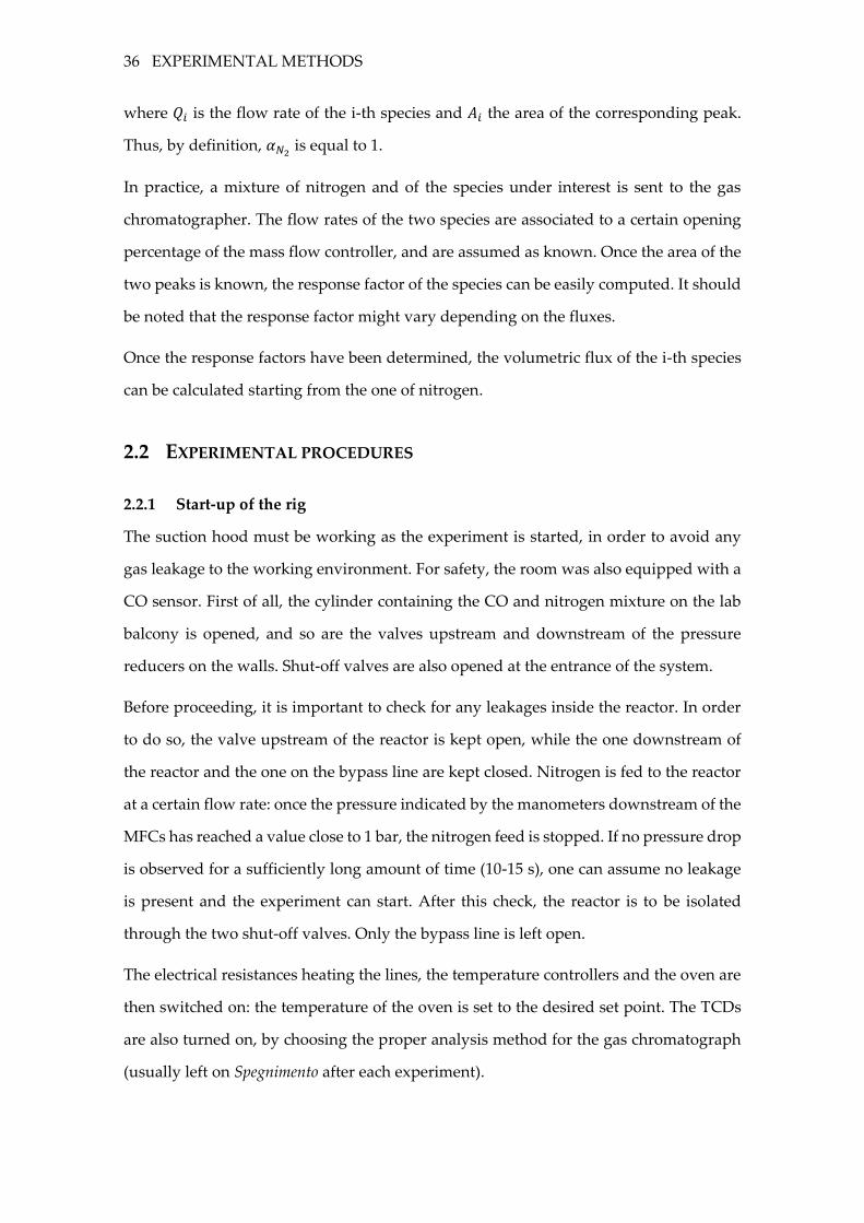
Figure 2.5: Brooks control unit.
Once the temperature of the lines has reached the proper set point value, the reactants
can be sent through the bypass line to the analysis section. In order to do so, the proper
openings are to be selected on the Brooks control unit (Figure 2.5). The total flow rate,
which is required for the estimation of the molar flow rates of the single species starting
from the data aquired from the gas chromatograph, is measured by means of a
stopwatch through the bubble flow meter. The flow rates of the single reactants can also
be measured as an additional check.
Through the data acquired by the chromatograph, it is possible to check whether the
actual composition reflects the nominal one. If not, the openings of the MFCs have to be
adjusted. Once the concentrations of the reactants are close to the desired ones and the
oven has reached the nominal temperature, the reactor line can be opened and the
bypass line is closed.
2.2.2 Execution of the experiment
Once the oven has reached the desired temperature and is stable, the products can be
injected into the GC for the analysis. When collecting the data, three injections were
usually performed and their results averaged in order to minimize the experimental
error. More in particular, by defining:
𝑓𝑖 =𝐴𝑖𝐴𝑁2
where 𝐴𝑖 is the area of the peak corresponding to the i-th species, and indicating as 𝑓1, 𝑓2
and 𝑓3 the values of such ratio for each injection, the volumetric flow rate of species i can
be calculated as:
38 EXPERIMENTAL METHODS
𝑄𝑖 = 𝛼𝑖𝑓1 + 𝑓2 + 𝑓3
3𝑄𝑁2
where 𝑄𝑁2 is the volumetric flow rate of nitrogen in NmL/min, which is assumed to be
constant throughout the whole experiment.
In the case of column B, there is no nitrogen peak. Instead, a macro-peak corresponding
to a CO, oxygen and nitrogen mixture is present. In order to quantify the flow rates of
the species detected by column B, the area of apparent nitrogen is calculated as:
𝐴𝑁2,𝑎𝑝𝑝𝐵 = 𝐴𝑚𝑎𝑐𝑟𝑜−𝑝𝑒𝑎𝑘
𝐵 ∙ 𝑥𝑁2
where 𝑥𝑁2 is the fraction of nitrogen in the macro-peak, calculated from the areas
obtained through column A (again, the average value of the three injections is taken):
𝑥𝑁2 =𝐴𝑁2𝐴
𝐴𝑁2𝐴 + 𝐴𝑂2
𝐴 + 𝐴𝐶𝑂𝐴
The molar flow in μmol/min and the molar fractions are given by:
�̇�𝑖 =𝑄𝑖
0.022414
𝑦𝑖 =�̇�𝑖
∑ �̇�𝑖𝑁𝐶𝑖=1
Starting from the composition, other quantities of interest can be calculated, such as the
conversion of CO and oxygen, and the selectivity of CO:
𝜒𝐶𝑂 =�̇�𝐶𝑂,𝑖𝑛 − �̇�𝐶𝑂
�̇�𝐶𝑂,𝑖𝑛
𝜒𝑂2 =�̇�𝑂2,𝑖𝑛 − �̇�𝑂2�̇�𝑂2,𝑖𝑛
𝑆𝐶𝑂2 =0.5(�̇�𝐶𝑂,𝑖𝑛 − �̇�𝐶𝑂)
�̇�𝑂2,𝑖𝑛 − �̇�𝑂2
In order to verify the quality of the experiments, carbon and oxygen balances were used
during the experiments. Such quantities are defined as the ratio between the carbon
(oxygen) atoms in the products divided by the converted carbon (oxygen) atoms, i.e.:
𝐵𝐶 =∑ �̇�𝑝𝑟𝑜𝑑,𝑖 ∙ 𝑛𝐶,𝑝𝑟𝑜𝑑,𝑖𝑁𝑃𝑖=1
∑ (�̇�𝑟𝑒𝑎𝑐𝑡𝑗,𝑖𝑛 − �̇�𝑟𝑒𝑎𝑐𝑡,𝑗) ∙ 𝑛𝐶,𝑟𝑒𝑎𝑐𝑡,𝑗𝑁𝑅𝑗=1
=�̇�𝐶𝑂2 ∙ 𝑛𝐶,𝐶𝑂2
(�̇�𝐶𝑂,𝑖𝑛 − �̇�𝐶𝑂) ∙ 𝑛𝐶,𝐶𝑂

EXPERIMENTAL PROCEDURES 39
𝐵𝑂 =∑ �̇�𝑝𝑟𝑜𝑑,𝑖 ∙ 𝑛𝑂,𝑝𝑟𝑜𝑑,𝑖𝑁𝑃𝑖=1
∑ (�̇�𝑟𝑒𝑎𝑐𝑡𝑗,𝑖𝑛 − �̇�𝑟𝑒𝑎𝑐𝑡,𝑗) ∙ 𝑛𝑂,𝑟𝑒𝑎𝑐𝑡,𝑗𝑁𝑅𝑗=1
=�̇�𝐶𝑂2 ∙ 𝑛𝐶𝑂2 + �̇�𝐻2𝑂 ∙ 𝑛𝐻2𝑂
(�̇�𝑂2,𝑖𝑛 − �̇�𝑂2) ∙ 𝑛𝑂,𝑂2
These quantities should be of course very close to 1. A balance greater than one means
that the amount of products is being overestimated, while a balance smaller than one
indicates its underestimation. The formation of parasitic species, such as solid carbon,
might also alter the value of the balances.
Once the data related to a certain nominal temperature have been collected, the set point
temperature of the oven can be increased up to the next desired value. The usual
temperature range used for the experiments was 100 °C-300 °C, at 20 °C intervals.
2.2.3 Axial temperature profiles (annular reactor)
In the case of the annular reactor, the axial temperature profile is also taken for both the
oven and the reactor – not only along the length the catalytic bed, but up to 1 cm
upstream and downstream of it. This is done by letting the thermocouples slide inside
the oven and the alumina tube two millimiters at a time, and by taking the corresponding
temperatures (indicated on the TIC). This measurement is of great importance, since the
reactor can be deemed isothermal only as long as the axial temperature gradient does
not exceed 5 °C/cm. The results obtained in the experiments are also indicated on the
plots not as a function of the nominal temperature, but as a function of the average
temperature of the bed.
Figure 2.6: Scheme of the thermocouples used for the measurement of the axial temperature profiles.
2.2.4 Shut-down of the rig
At the end of the experiment, the set point of the oven is set to zero. As the temperature
starts to decrease, the oven can be switched off. The mass flow controllers and shut-off
valves associated to all the reactants but nitrogen are then closed: since both air and a
large excess of hydrogen are present, it is important to close air first in order to avoid the
40 EXPERIMENTAL METHODS
formation of a flammable mixture. Nitrogen is left flowing inside the reactor in order to
clean it: after a while, it is possible to open the bypass line and isolate the reactor by
closing the shut-off valves on the reactor line. Nitrogen can then be closed, and so can
the inlet valves, the valves associated to the pressure reducers and the CO-nitrogen
cylinder outside of the laboratory.
Finally, the heating tapes are turned off through the TIC and the GC is set to the
Spegnimento method.
2.3 CATALYST CHARACTERIZATION
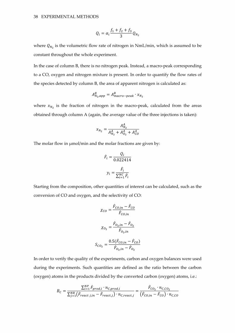
2.3.1 Main features of the catalyst
The catalyst used in the experiments of this Thesis work is a commercial one, provided
by ICI Caldaie S.p.A. in the form of spherical pellets. It was never used as such: it was
used before in the form of a powder in fixed bed reactors, then as a deposited slurry in
the annular reactor. The catalyst is based on a platinum group metal (PGM), presumably
supported on alumina, and is said to require no pre-activation on the product sheet.
Figure 2.7: Catalytic pellets observed at the optical microscope. The pellet on the right was cut in half for the
measurement of the thickness.
The average diameter of the spheres and the thickness of the active phase were evaluated
through the observation of a selected number of spheres at the optical microscope. In a
first set of measurements, four spheres at a time were observed and photographed. The
cross section of the spheres was then estimated starting from the photographs, by
knowing the enlargement scale (60x). The average external diameter could be then
calculated from the cross section. In a second set of observations, the same procedure
was carried out, but the spheres were before cut in half by means of sharp blades. This
CATALYST CHARACTERIZATION 41
time, the thickness of the active phase could be assessed, again by knowing the
enlargement scale (200x). Further details are reported in [30].
The average mass of the spheres was also estimated by means of a precision scale.
Starting from the mass and the diameter of the pellets, the density of the catalyst can be
simply calculated as:
𝜌𝑐𝑎𝑡 =𝑚𝑐𝑎𝑡
𝜋6𝑑𝑠𝑝ℎ𝑒𝑟𝑒3
The properties of the catalyst are reported in the following table:
Average external
diameter [mm]
Thickness of the
active phase [mm] Mass [kg] Density [kg/m3]
2.014 0.095 4.31∙10−6 1007.3
Table 2.1: Properties of the catalyst pellets.
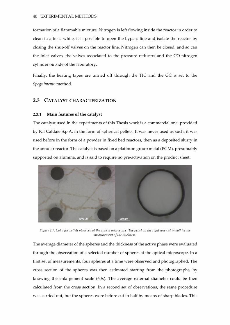
Both the pellets and the powders were also characterized from a morphological point of
view by means of a BET analysis (Micromeritics TriStar 3000) and of mercury intrusion
porosimetry (Micromeritics AutoPore V). The first analysis had the aim of quantifying
the surface area of the sample, while the second one was used to quantify the porosity,
the pore volume and the pore size distribution. The results of the analyses are reported
in the following tables.
From the BET:
Spheres Powder
BET surface area
[m2/g] 175.4 176.0
Table 2.2: Results of BET.
From Hg porosimetry:
Spheres Powder
Porosity [%] 69.5% 82.7%
Total pore area
[m2/g] 307.5 245.7
Average pore
diameter [Å] 83.3 197.5
Table 2.3: Results of mercury porosimetry.
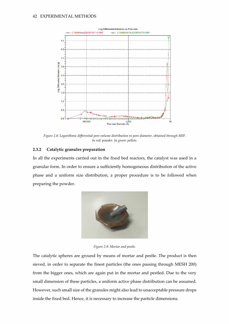
42 EXPERIMENTAL METHODS
Figure 2.8: Logarithmic differential pore volume distribution vs pore diameter, obtained through MIP.
In red: powder. In green: pellets.
2.3.2 Catalytic granules preparation
In all the experiments carried out in the fixed bed reactors, the catalyst was used in a
granular form. In order to ensure a sufficiently homogeneous distribution of the active
phase and a uniform size distribution, a proper procedure is to be followed when
preparing the powder.
Figure 2.9: Mortar and pestle.
The catalytic spheres are ground by means of mortar and pestle. The product is then
sieved, in order to separate the finest particles (the ones passing through MESH 200)
from the bigger ones, which are again put in the mortar and pestled. Due to the very
small dimension of these particles, a uniform active phase distribution can be assumed.
However, such small size of the granules might also lead to unacceptable pressure drops
inside the fixed bed. Hence, it is necessary to increase the particle dimensions.
CATALYST CHARACTERIZATION 43
Figure 2.10: Hydraulic press.
The fines are first compacted in a tablet-making machine. The particles are put between
two metal disks into a hollow cylinder, which is then set on a hydraulic press. The
pressure applied through the press pushes the disks and compacts the fines in a tablet-
like shape. Finally, the tablets are ground and sieved. This time, larger particles are
collected (MESH 140-200, between 0.074 and 0.105 mm).
The same procedure is followed for the preparation of the powders which are required
for the slurry.
2.3.3 Slurry preparation
In the case of the annular reactor, the catalyst is present on an alumina tube in the form
of a thin coating, obtained from the deposition of a slurry. The slurry is a dispersion of
alumina powders in water: these were obtained from the commerical catalyst pellets
through the same procedure described in 2.3.2. For the slurry to be stable, a strong acid
is also required: nitric acid was used in the preparation. It works by charging the surface
of the particles, but it is also consumed in an oxide dissolution reaction [31].
For the subsequent deposition step to be effective, the rheological properties of the slurry
(in particular its viscosity) should be adequate. These are strongly influenced by both
the H2O/powder and the HNO3/powder ratios. Initially, ratios of 1.4 mL of distilled
water per gram of powder and 1.7 mmol of HNO3 per gram of powder were chosen.
44 EXPERIMENTAL METHODS
Indeed, this was found to be the optimal composition in previous works with Rh-
impregnated powders [32].
Starting from a given mass of powders (in this case, 5.4125 g), the corresponding amount
of HNO3 is given by (in grams):
𝑚𝐻𝑁𝑂3 =1.7
1000∙ 𝑚𝑝𝑜𝑤𝑑𝑒𝑟𝑠 ∙ 𝑀𝑊𝐻𝑁𝑂3
Nitric acid was used as a 65% w/w concentrated solution. Thus,
𝑚𝑠𝑜𝑙𝑢𝑡𝑖𝑜𝑛 =𝑚𝐻𝑁𝑂3
0.65
Finally, the required amount of water to be added is given by:
𝑚𝑤𝑎𝑡𝑒𝑟 =1.4
1000∙ 𝑚𝑝𝑜𝑤𝑑𝑒𝑟𝑠 ∙ 𝜌𝑤𝑎𝑡𝑒𝑟 − (1 − 0.65) ∙ 𝑚𝑠𝑜𝑙𝑢𝑡𝑖𝑜𝑛
During the dip-coating procedure, it was observed that the preparation dried on the
alumina tube without sticking to it. Hence, it was necessary to add a further amount of
water to the mixture (≃4 g) in order for it to acquire the proper viscosity.
The slurry is then put in a plastic container with zirconia balls, whose mass is 8 times the
one of the powders, and subjected to a 24-hour long ball milling procedure: the plastic
container is put inside a metallic cylinder, then set on two counter-rotating cylinders,
revolving at a constant speed of 40 rpm and driven by an electrical motor. This step is
required to obtain a homogeneous dispersion.
Figure 2.11: Ball milling.
CATALYST CHARACTERIZATION 45
2.3.4 Dip coating
For the deposition of the catalytic layer on the alumina tube, a procedure named dip
coating is followed. Aim of this step is to obtain a uniform, well-adherent layer of catalyst
on the alumina tube.
For this reason, before proceeding, the surface over which the catalyst is to be deposited
is covered in primer: this treatment results in an increase of the superficial roughness,
and favours the adherence of the deposited layers. In order to do so, the alumina tube is
immersed into a graduated cylinder containing the primer, then dried for 30 minutes at
ambient temperature. Teflon tape is used to isolate the catalytic bed from the rest of the
tube. After this preliminary operation, the actual dip coating procedure can be carried
out.
The slurry is put inside a graduated cylinder. Then, the alumina tube is attached to a
vertical slide, and carefully immersed into the cylinder at a constant speed. After being
left inside the solution for a while, the tube is pulled up, again at a costant speed. The
withdrawal velocity has an effect on the thickness of the coating. To remove the solvent,
the tube is dried in the oven for 10 minutes, at 280 °C. This procedure is called flash drying
and guarantees a fast evaporation and good adhesion of the catalyst layer.
After both the deposition of the primer and the one of the catalyst, the tube is weighted
by means of a precision scale, repeating the measurement at least three times. At the end
of the procedure, the catalyst load can be calculated as:
𝑚𝑐𝑎𝑡 = 𝑚𝑡𝑢𝑏𝑒+𝑐𝑎𝑡+𝑝𝑟𝑖𝑚𝑒𝑟 −𝑚𝑡𝑢𝑏𝑒+𝑝𝑟𝑖𝑚𝑒𝑟
One tube was prepared and used for this Thesis work. Here are reported its properties.
Name
Mass of catalyst
[mg]
Length of the
catalytic bed [cm]
V1 14.3 2
Table 2.4: Properties of tube V1.
46 EXPERIMENTAL METHODS
2.4 THERMODYNAMICS
2.4.1 Introduction
The main reactions which can take place inside a PrOx reactor are CO and hydrogen
oxidation: oxidations are typically strongly exothermic reactions, for which the
equilibrium conversion is expected to decrease at increasing temperatures. Water gas
shift, which is also exothermic, can in principle take place in the system: in particular,
the reaction is thermodynamically favoured in the whole range of temperatures used in
the experiments, with an equilibrium constant decreasing as the temperature increases.
Methanation might also in theory take place in the system: however, the formation of
methane was never observed. For this reason, this species was not taken into account
while calculating the equilibrium state.
During the experiments, the conversion of CO went quite often above the equilibrium
value at higher temperatures. While this might seem a violation of the thermodynamic
constraint at first, it is actually related to the occurrence of the fast, non-equilibrated
oxidation reactions. The decrease in the conversion of CO at high temperatures can be
explained through the reverse water gas shift reaction, converting part of the produced
CO2 into CO. The reaction is slower than the oxidations, and takes place only as all the
oxygen has been consumed.
For each test, the equilibrium composition was calculated and inserted into the graphs
as a dashed line. In particular, STANJAN Chemical Equilibrium Calculator [33] was
used to evaluate the equilibrium state of the mixture, treated as an ideal mixture of ideal
gases. It is worth noticing that the code does not consider liquid and solid species in the
calculations. STANJAN finds the equilibrium composition by minimizing the Gibbs’ free
energy of the mixture, using temperature, pressure and the inlet composition as inputs
for the calculation. Carbon dioxide and water were considered as the only possible
products.
2.4.2 Minimization of Gibbs’ free energy
Determining the equilibrium state of a system subject to the constraint of constant
temperature and pressure means minimizing the Gibbs’ free energy of the mixture [34].
Hence, its differential must be zero:
THERMODYNAMICS 47
𝑑𝐺𝑇,𝑃 =∑𝜇𝑖𝑑𝑛𝑖
𝑁𝐶
𝑖=1
= 0 (2.1)
For the sake of brevity, a system with
𝑁𝑅 = 𝑁𝐶 − 𝑟𝑎𝑛𝑘(𝑨) (2.2)
where 𝑁𝐶 is the number of components and 𝑨 is the matrix with an atomic species for
each row and a molecular species for each column, will be considered. However, the
approach can be simply generalized to complex systems.
Due to the stoichiometric constraint, the ratio between the variation in the number of
moles of a certain species and its stoichiometric coefficient in a reaction must be the same
for all the species taking part in such reaction. Hence, by defining
𝑑𝜆 =𝑑𝑛𝑖𝜈𝑖
(2.3)
as the extent of the reaction, it follows that:
∑𝜇𝑖𝑑𝑛𝑖
𝑁𝐶
𝑖=1
=∑𝜇𝑖𝜈𝑖𝑑𝜆
𝑁𝐶
𝑖=1
= 0 (2.4)
Since 𝑑𝜆 is arbitrary, the equation can be rewritten as:
∑𝜇𝑖𝜈𝑖
𝑁𝐶
𝑖=1
= 0 (2.5)
𝜇𝑖 is the chemical potential of species i. By exploiting Lewis’ definition of fugacity:
𝑑𝜇𝑖,𝑇 = 𝑅𝑇𝑑𝑙𝑛𝑓𝑖 (2.6)
and integrating between a reference state and a generic one, it follows that:
𝜇𝑖(𝑇, 𝑃, 𝒚) = 𝜇𝑖(𝑇, 𝑃𝑟𝑒𝑓) + 𝑅𝑇𝑙𝑛 (
𝑓𝑖(𝑇, 𝑃, 𝒚)
𝑓𝑖(𝑇, 𝑃𝑟𝑒𝑓))
𝜇𝑖(𝑇, 𝑃, 𝒚) = 𝜇𝑖(𝑇, 𝑃𝑟𝑒𝑓) + 𝑅𝑇𝑙𝑛(𝑎𝑖(𝑇, 𝑃, 𝑃𝑟𝑒𝑓 , 𝒚))
(2.7)
where 𝑎𝑖 is the activity of the i-th species. The fugacity of a species i in a mixure can be
expressed as:
𝑓𝑖(𝑇, 𝑃, 𝒚) = 𝑃�̂�𝑖(𝑇, 𝑃, 𝒚)𝑦𝑖 (2.8)
48 EXPERIMENTAL METHODS
For a gas, the reference state which is considered in the estimation of the activity, is an
ideal pure gas at 1 bar. Hence,
𝑎𝑖(𝑇, 𝑃, 𝑃𝑟𝑒𝑓 , 𝒚) =𝑃𝑦𝑖
1[𝑏𝑎𝑟]= 𝑃𝑦𝑖 (2.9)
Since the mixture is treated as an ideal mixure of ideal gases (only gaseous species are
present, and the working pressure is far from the critical pressures of the species), it
follows that:
𝑓𝑖(𝑇, 𝑃, 𝒚) = 𝑃�̂�𝑖(𝑇, 𝑃, 𝒚)𝑦𝑖 = 𝑃𝑦𝑖 (2.10)
Going back to equation 2.5,
𝑑𝐺𝑇,𝑃 =∑𝜈𝑖𝜇𝑖(𝑇, 𝑃𝑟𝑒𝑓)
𝑁𝐶
𝑖=1
+ 𝑅𝑇∑𝜈𝑖𝑙𝑛(𝑎𝑖(𝑇, 𝑃, 𝑃𝑟𝑒𝑓 , 𝒚))
𝑁𝐶
𝑖=1
= 0 (2.11)
Re-organising,
∑𝜈𝑖𝜇𝑖(𝑇, 𝑃𝑟𝑒𝑓)
𝑁𝐶
𝑖=1
+ 𝑅𝑇∏(𝑎𝑖(𝑇, 𝑃, 𝑃𝑟𝑒𝑓 , 𝒚))𝜈𝑖
𝑁𝐶
𝑖=1
= 0 (2.12)
It is worth remarking that the reference state for the two terms must be the same. Since
the chemical potential of a pure compound is equal to its molar Gibbs’ free energy, the
first term can be re-written as:
∑𝜈𝑖𝜇𝑖(𝑇, 𝑃𝑟𝑒𝑓)
𝑁𝐶
𝑖=1
=∑𝜈𝑖𝑔𝑖(𝑇, 𝑃𝑟𝑒𝑓)
𝑁𝐶
𝑖=1
= 𝛥𝐺°𝑅(𝑇, 𝑃𝑟𝑒𝑓) (2.13)
where 𝛥𝐺°𝑅 is the variation of Gibbs’ free energy associated to the complete
transformation of a stoichiometric amount of reactants into products, at reference
conditions.
By going back to equation 2.12 the second term is usually expressed as:
∏(𝑎𝑖(𝑇, 𝑃, 𝑃𝑟𝑒𝑓 , 𝒚))𝜈𝑖
𝑁𝐶
𝑖=1
= 𝐾𝑒𝑞 (2.14)
where 𝐾𝑒𝑞 is the equilibrium constant for the reaction. Thus, relation 2.12 becomes:
𝐾𝑒𝑞 = exp (−𝛥𝐺°𝑅(𝑇, 𝑃𝑟𝑒𝑓)
𝑅𝑇) =∏(𝑃𝑦𝑖)
𝜈𝑖
𝑁𝐶
𝑖=1
(2.15)
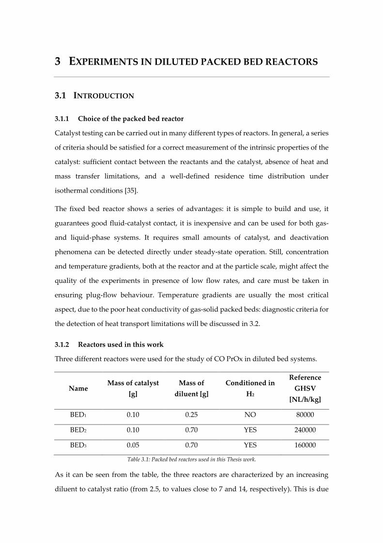
3 EXPERIMENTS IN DILUTED PACKED BED REACTORS
3.1 INTRODUCTION
3.1.1 Choice of the packed bed reactor
Catalyst testing can be carried out in many different types of reactors. In general, a series
of criteria should be satisfied for a correct measurement of the intrinsic properties of the
catalyst: sufficient contact between the reactants and the catalyst, absence of heat and
mass transfer limitations, and a well-defined residence time distribution under
isothermal conditions [35].
The fixed bed reactor shows a series of advantages: it is simple to build and use, it
guarantees good fluid-catalyst contact, it is inexpensive and can be used for both gas-
and liquid-phase systems. It requires small amounts of catalyst, and deactivation
phenomena can be detected directly under steady-state operation. Still, concentration
and temperature gradients, both at the reactor and at the particle scale, might affect the
quality of the experiments in presence of low flow rates, and care must be taken in
ensuring plug-flow behaviour. Temperature gradients are usually the most critical
aspect, due to the poor heat conductivity of gas-solid packed beds: diagnostic criteria for
the detection of heat transport limitations will be discussed in 3.2.
3.1.2 Reactors used in this work
Three different reactors were used for the study of CO PrOx in diluted bed systems.
Name Mass of catalyst
[g]
Mass of
diluent [g]
Conditioned in
H2
Reference
GHSV
[NL/h/kg]
BED1 0.10 0.25 NO 80000
BED2 0.10 0.70 YES 240000
BED3 0.05 0.70 YES 160000
Table 3.1: Packed bed reactors used in this Thesis work.
As it can be seen from the table, the three reactors are characterized by an increasing
diluent to catalyst ratio (from 2.5, to values close to 7 and 14, respectively). This is due
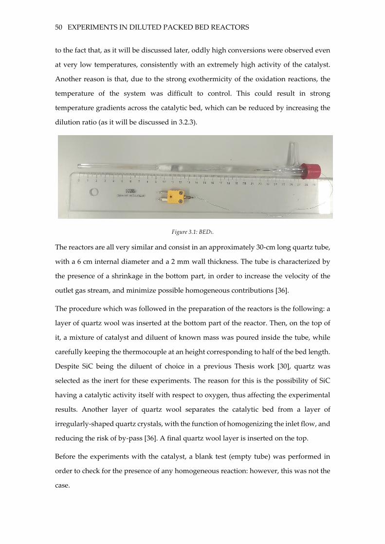
50 EXPERIMENTS IN DILUTED PACKED BED REACTORS
to the fact that, as it will be discussed later, oddly high conversions were observed even
at very low temperatures, consistently with an extremely high activity of the catalyst.
Another reason is that, due to the strong exothermicity of the oxidation reactions, the
temperature of the system was difficult to control. This could result in strong
temperature gradients across the catalytic bed, which can be reduced by increasing the
dilution ratio (as it will be discussed in 3.2.3).
Figure 3.1: BED1.
The reactors are all very similar and consist in an approximately 30-cm long quartz tube,
with a 6 cm internal diameter and a 2 mm wall thickness. The tube is characterized by
the presence of a shrinkage in the bottom part, in order to increase the velocity of the
outlet gas stream, and minimize possible homogeneous contributions [36].
The procedure which was followed in the preparation of the reactors is the following: a
layer of quartz wool was inserted at the bottom part of the reactor. Then, on the top of
it, a mixture of catalyst and diluent of known mass was poured inside the tube, while
carefully keeping the thermocouple at an height corresponding to half of the bed length.
Despite SiC being the diluent of choice in a previous Thesis work [30], quartz was
selected as the inert for these experiments. The reason for this is the possibility of SiC
having a catalytic activity itself with respect to oxygen, thus affecting the experimental
results. Another layer of quartz wool separates the catalytic bed from a layer of
irregularly-shaped quartz crystals, with the function of homogenizing the inlet flow, and
reducing the risk of by-pass [36]. A final quartz wool layer is inserted on the top.
Before the experiments with the catalyst, a blank test (empty tube) was performed in
order to check for the presence of any homogeneous reaction: however, this was not the
case.
INTRODUCTION 51
3.1.3 Operating conditions
For the three beds, a reference composition of 40% hydrogen, 1% CO, 1% O2 and
complementary nitrogen was selected. The amounts of CO and O2 reflect the ones which
can be expected in a real CO PrOx reactor for the application in fuel cell systems: despite
being 0.5% O2 the stoichiometric concentration, oxygen is usually fed to the preferential
oxidation stage in sovrastoichiometric amounts, in order to guarantee a thorough
consumption of CO. The amount of hydrogen was selected referring to the outlet
composition of experiments previously conduted on the water gas shift reaction [37]. In
the literature, experiments have been carried out at many different possible H2
concentrations. In any case, one should expect a large excess of hydrogen to be present
with respect to the other reactants (typical H2/CO ratios exceed 100:1 at the outlet of the
water gas shift stage and can increase up to 50000:1 as the PrOx reaction proceeds to
completion [5]).
Initially, 40 °C-300 °C was the temperature range of choice, since CO PrOx reactors are
usually operated at low temperatures. However, even from the very first experiments, it
was clear that a reliable investigation of the 40 °C-100°C temperature range was not
feasible. This could be observed not only from the poor reproducibility of data at low
temperatures, but also from the sudden temperature increase at the beginning of every
experiment. The set point of the oven was set equal to 40 °C before opening the reactor:
then, as the reactant mixture was sent on the bed, the temperature of the catalyst
increased up to a value which depended on the experimental conditions.
This made it necessary to follow a specific procedure: in order to get to the desired
temperature, the set point of the oven was increased 5 °C at a time, every twenty seconds,
from 0 °C up to the first temperature, in order to avoid abrupt temperature increases. It
should be noted that the lines inside which the reactants were fed to the reactor were
heated up to 120 °C, a temperature which is much higher than the set point of the oven:
however, keeping the heating tapes off and turning them on only at the beginning of the
experiment did not change the situation. Hence, the temperature increase is probably
related to the strong exothermicity of both the CO and the H2 oxidation reactions and to
the poor capability of the packed bed of efficiently dissipate the reaction heat. This was
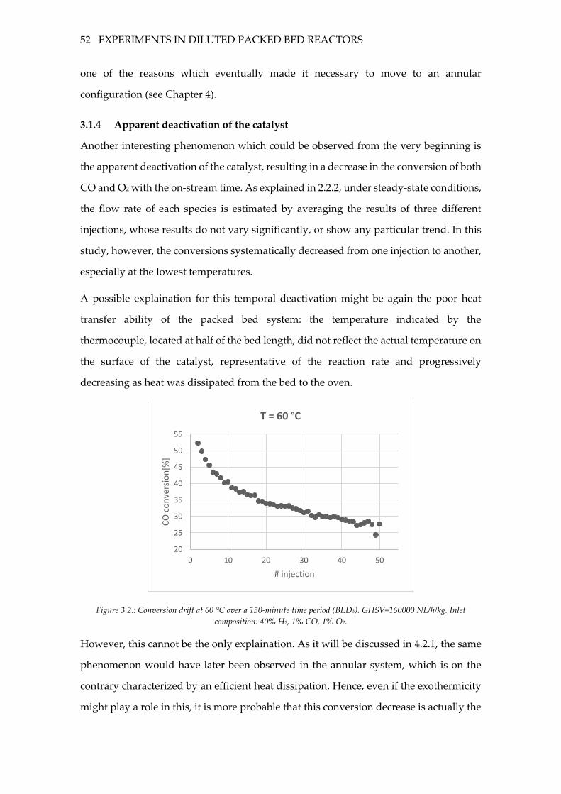
52 EXPERIMENTS IN DILUTED PACKED BED REACTORS
one of the reasons which eventually made it necessary to move to an annular
configuration (see Chapter 4).
3.1.4 Apparent deactivation of the catalyst
Another interesting phenomenon which could be observed from the very beginning is
the apparent deactivation of the catalyst, resulting in a decrease in the conversion of both
CO and O2 with the on-stream time. As explained in 2.2.2, under steady-state conditions,
the flow rate of each species is estimated by averaging the results of three different
injections, whose results do not vary significantly, or show any particular trend. In this
study, however, the conversions systematically decreased from one injection to another,
especially at the lowest temperatures.
A possible explaination for this temporal deactivation might be again the poor heat
transfer ability of the packed bed system: the temperature indicated by the
thermocouple, located at half of the bed length, did not reflect the actual temperature on
the surface of the catalyst, representative of the reaction rate and progressively
decreasing as heat was dissipated from the bed to the oven.
Figure 3.2.: Conversion drift at 60 °C over a 150-minute time period (BED3). GHSV=160000 NL/h/kg. Inlet
composition: 40% H2, 1% CO, 1% O2.
However, this cannot be the only explaination. As it will be discussed in 4.2.1, the same
phenomenon would have later been observed in the annular system, which is on the
contrary characterized by an efficient heat dissipation. Hence, even if the exothermicity
might play a role in this, it is more probable that this conversion decrease is actually the
20
25
30
35
40
45
50
55
0 10 20 30 40 50
CO
co
nve
rsio
n[%
]
# injection
T = 60 °C
DIAGNOSTIC CRITERIA FOR HEAT TRANSPORT LIMITATIONS 53
visible effect of very slow stabilization dynamics, associated to an extremely low reaction
rate. The phenomenon is also cited in some works [5], [22], [38].
Some authors [39] state that the significant deactivation of the catalyst with the time of
stream is not related to a modification in the intrinsic activity of the catalyst (since the
pseudo-first-order kinetic contant of the reaction is more or less unchanging), but to a
decrease in the surface concentration of CO2 intermediates, related to the available active
Pt sites. The initial activity of the catalyst could be completely restored by treating the
catalyst in a hydrogen stream.
Other authors [18] confirmed that this apparent deactivation is perfectly reversible:
indeed, the initial reaction rates and selectivity were restored simply by treating the
sample in a flow of He at 623 K for 900 s. As a possible explaination for the phenomenon,
the authors assume the progressive increase in chemisorbed CO coverages up to the
steady-state value, in the presence of other species: the kinetic consequences can be
considered equivalent to a gradual increase in the adsorption constant of CO.
In later experiments in the diluted packed bed system, injections were performed for up
to one hour at the first temperature in order to obtain at least a partial stabilization of the
system. This effect was investigated in more depth in BED3 (3.3.3).
3.2 DIAGNOSTIC CRITERIA FOR HEAT TRANSPORT LIMITATIONS
3.2.1 Introduction
In principle, kinetic data should be collected in fixed beds operated as integral reactors
under rigorous isothermal conditions. However, the presence of temperature gradients
can cause a significant deviation from the ideal isothermal, plug-flow behaviour in fixed
bed reactors [40], thus altering the experimental results. Thermal gradients might be
intraparticle, thus related to the heat transfer inside the catalytic pellet; interphase,
between the bulk of the gas phase and the surface of the solid, possibly at a much higher
temperature due the presence of an exothermic reaction; interparticle, between the fluid
and the wall.
A criterion to prove the absence of intraparticle temperature gradients was developed
by Anderson, by imposing a <5% deviation of the observed rate from the isothermal one.
54 EXPERIMENTS IN DILUTED PACKED BED REACTORS
However, Fulton and Crosser proved that for gas-solid systems the intraparticle heat
transfer resistance is negligible with respect to the interphase one. Thus, the particle itself
can be usually deemed isothermal. Diagnostic criteria similar to the one of Anderson can
be derived for the interphase, and interparticle transport.
3.2.2 Interphase transport
A criterion [40] for the detection of interphase heat transfer limitations can be obtained
by the perturbation approach. By assuming an Arrhenius-type dependence on the
temperature for the reaction rate
ℜ = 𝐴𝑒−𝐸 𝑅𝑇⁄ 𝑓(𝑐) (3.1)
then the reaction rate at a temperature 𝑇 close to 𝑇0 (the temperature of the bulk fluid)
can be expressed through a Taylor expansion around 𝑇0:
ℜ = ℜ0 (1 +𝑇 − 𝑇0𝑇0
𝐸
𝑅𝑇0) (3.2)
where ℜ0 is the reaction rate at 𝑇0. By neglecting heat conduction to adjacent touching
particles, the energy balance for the particle can be written as:
𝑞ℜ4𝜋
3(𝑟𝑝)
3 = ℎ(𝑇 − 𝑇0)4𝜋(𝑟𝑝)2 (3.3)
where 𝑞 is the absolute value of the heat of the reaction, 𝑟𝑝 the particle radius and ℎ the
heat-solid gas transfer coefficient. Combining the two equations gives:
ℜ
ℜ0= 1 +
𝑞ℜ𝑟𝑝𝐸
3ℎ𝑇02𝑅
(3.4)
The observed rate ℜ, calculated from experimental data, must not deviate from the one
calculated at the bulk gas temperature 𝑇0 by more than 5%, in order for the system to be
deemed isothermal. The resulting criterion to be respected is the following, valid no
matter the presence of intraparticle diffusional limitations:
𝑞ℜ𝑟𝑝
ℎ𝑇0< 0.15
𝑅𝑇0𝐸
(3.5)
Interphase transfer limitations can thus be expected in the case of high heats of reaction,
or for systems operating at low Reynolds numbers (and thus low ℎ).
DIAGNOSTIC CRITERIA FOR HEAT TRANSPORT LIMITATIONS 55
3.2.3 Interparticle transport
A rigorous derivation of axial and radial temperature profiles would involve the
resolution of partial differential equations: numerical solutions yield approximately
parabolic radial temperature profiles, while the temperature along the axis increases up
to a maximum at the hot-spot and then decreases gradually until reaching again the wall
temperature 𝑇𝑤.
A criterion for the detection of a radial heat transport limitation was also proposed in
[40]. By referring to a bed with a sufficiently high length to particle diameter ratio, axial
conduction can be neglected. Hence, the energy balance at the hotspot can be written as:
𝑘𝑒 (𝑑2𝑇
𝑑𝑟2+1
𝑟
𝑑𝑇
𝑑𝑟) = (−∆𝐻)
(1 − 휀)
(1 − 𝑏)ℜ = (−∆𝐻)ℜ′ (3.6)
where the sensible term has been neglected. Moreover, the local rate is defined as:
ℜ′ =(1 − 휀)
(1 − 𝑏)ℜ (3.7)
where 휀 is the void fraction and 𝑏 the dilution (inert to catalyst) ratio. By defining the
dimensionless temperature and radius (𝑅0 is the radius of the reactor):
𝜃 =𝐸(𝑇 −𝑇𝑤)
𝑅𝑇𝑤2 (3.8a)
𝑢 =𝑟
𝑅0 (3.8b)
the analytical solution derived for the radial temperature profiles can be expressed as:
𝜃 − 𝜃𝑚𝑎𝑥 = −2ln(𝐵𝑢2 + 1) (3.9a)
𝐵 =𝛿
8exp(|𝜃𝑚𝑎𝑥|) (3.9b)
𝛿 =(−∆𝐻)ℜ′𝑤𝑅0
2𝐸
𝑘𝑒𝑇𝑤2𝑅
(3.9c)
where 𝜃𝑚𝑎𝑥 is the maximum dimensionless temperature at the hotspot.
By imposing the boundary condition 𝑢 = 1 for 𝜃 = 0 (i.e.: the temperature is equal to 𝑇𝑤
at the wall), the following relation is derived:
𝛿 = 8[exp(−0.5|𝜃𝑚𝑎𝑥|) − exp(−|𝜃𝑚𝑎𝑥|)] (3.10)
56 EXPERIMENTS IN DILUTED PACKED BED REACTORS
When the radial temperature gradient is just starting to become significant, 𝛿 is small
and so is 𝐵. Hence, the following approximation can be used:
𝜃 − 𝜃𝑚𝑎𝑥 = −2𝐵𝑢2 (3.11)
Finally, the following expression for 𝜃𝑚𝑎𝑥 can be obtained:
𝜃𝑚𝑎𝑥 =𝛿 4⁄
1 − 𝛿 4⁄≈ 𝛿 4⁄ (3.12)
The heat transfer resistance at the wall is usually not negligible in small laboratory
reactors (𝑅0 𝑟𝑝⁄ < 100), and aggravates the interparticle heat transport. In this case, the
proper boundary condition is given by:
𝑘𝑒𝑑𝑇
𝑑𝑟|𝑟=𝑅0
= ℎ𝑤(𝑇 − 𝑇𝑤)|𝑟=𝑅0 (3.13)
In adimensional terms,
𝑑𝜃
𝑑𝑢|𝑢=1
=ℎ𝑤𝑅0𝑘𝑒
𝜃|𝑢=1 =𝐵𝑖𝑤2
𝑅0𝑟𝑝𝜃|𝑢=1 (3.14)
where 𝐵𝑖𝑤 =ℎ𝑤𝑑𝑝
𝑘𝑒 is the so-called Biot number, an adimensional quantity expressing the
ratio between the heat transfer at the wall and the one at the center of the bed.
Using this boundary condition, the following expression is obtained for 𝜃𝑚𝑎𝑥:
𝜃𝑚𝑎𝑥 =𝛿
4(1 +
4𝑘𝑒ℎ𝑤𝑅0
) =𝛿
4(1 +
8
𝐵𝑖𝑤
𝑟𝑝
𝑅0) (3.15)
which is negative in the case of endothermic reactions.
Finally, the effect of the radial gradients on the reaction rate can be assessed by
substituting eqs. 3.8a and 3.11 into equation 3.2, and integrating across the cross section:
𝜋(1)2ℜ′̅̅ ̅ = ℜ′𝑤∫ (1 + 𝜃𝑚𝑎𝑥 − 2𝐵𝑢2
1
0
)2𝜋𝑢𝑑𝑢 (3.16)
where ℜ′̅̅ ̅ is the average reaction rate at the cross section of the hot-spot. It follows that:
ℜ′̅̅ ̅
ℜ′𝑤= 1 + 𝜃𝑚𝑎𝑥 − 𝐵 (3.17)
The average rate ℜ′̅̅ ̅ should not deviate from ℜ′𝑤 (the local rate at 𝑇𝑤) by more than 5%,
in order for the system to be deemed isothermal. Hence, the following relationship must
hold:
DIAGNOSTIC CRITERIA FOR HEAT TRANSPORT LIMITATIONS 57
𝑞ℜ′̅̅ ̅𝑅0
2
𝑘𝑒𝑇𝑤<
0.4𝑅𝑇𝑤 𝐸⁄
(1 + 8 𝑟𝑝 𝑅0𝐵𝑖𝑤⁄ ) (3.18)
which simplifies to
𝑞ℜ′̅̅ ̅𝑅0
2
𝑘𝑒𝑇𝑤< 0.4
𝑅𝑇𝑤𝐸
(3.19)
if the heat transfer resistance at the wall is negligible.
Reducing the reactor diameter (present at the numerator in the left hand side in the
interparticle criterion, but also affecting the gas velocity and thus the transport
properties) and the particle radius might help in the minimization of heat transport
limitations. Diluting the bed is also beneficial towards the reduction of radial
temperature gradients, since it results in a smaller rate per unit volume: however,
dilution might significantly decrease the gas velocity and be the source of undesired
bypass phenomena.
3.2.4 Estimation of the transport properties
𝑘𝑒 is the effective thermal conductivity across the bed. It is usually expressed as the sum
of two terms: a static contribution and a dynamic one, related to the gas-solid interaction:
𝑘𝑒𝑘𝑔=𝑘𝑠𝑡𝑎𝑡𝑘𝑔
+𝑘𝑐𝑜𝑛𝑣𝑘𝑔
(3.20)
where 𝑘𝑔 is the thermal conductivity of the gas mixture. For 𝑅𝑒 > 40, the static
contribution can be calculated as (𝑘𝑝 is the thermal conductivity of the particle) [41]:
𝑘𝑠𝑡𝑎𝑡𝑘𝑔
= 휀𝑏 +1 − 휀𝑏
0.220휀𝑏2 + 2/3
𝑘𝑔𝑘𝑝
(3.21)
The dynamic contribution is usually defined as:
𝑘𝑐𝑜𝑛𝑣𝑘𝑔
=1
𝑃𝑒𝑟𝑖𝑓𝑅𝑒𝑝𝑃𝑟 (3.22)
where
𝑅𝑒𝑝 =𝜌𝑔𝑣𝑑𝑝
𝜇𝑔 (3.23)
𝑃𝑟 =𝜇𝑔𝑐𝑝,𝑔
𝑘𝑔 (3.24)
58 EXPERIMENTS IN DILUTED PACKED BED REACTORS
𝑃𝑒𝑟𝑖𝑓 = 8.65 [1 + 19.4 (𝑑𝑝
𝑑𝑡)] (3.25)
The density of the gaseous mixture is calculated through the ideal gas law and 𝑐𝑝,𝑔 as
∑𝑥𝑖𝑐𝑝,𝑖, while both the viscosity and the conductivity of the gaseous mixture have been
calculated by using the ASALI [42] code.
The heat transfer coefficient at the wall is also the sum of two contributions:
ℎ𝑤 = ℎ𝑤,𝑠𝑡𝑎𝑡 + ℎ𝑤,𝑐𝑜𝑛𝑣 (3.26)
where ℎ𝑤,𝑠𝑡𝑎𝑡 can be calculated as [41]:
ℎ𝑤,𝑠𝑡𝑎𝑡𝑑𝑝
𝑘𝑔= 2휀𝑏 +
1 − 휀𝑏
0.0024 (𝑑𝑡𝑑𝑝)1.58
+ 1/3𝑘𝑔𝑘𝑝
(3.27)
and the dynamic contribution as:
{
ℎ𝑤,𝑐𝑜𝑛𝑣 = 0.0835
𝑘𝑔
𝑑𝑝𝑅𝑒𝑝
0.91 (𝑃𝑟
𝑃𝑟𝑎𝑖𝑟,80°𝐶)
1/3
for𝑅𝑒𝑝 < 1200
ℎ𝑤,𝑐𝑜𝑛𝑣 = 1.23𝑘𝑔
𝑑𝑝𝑅𝑒𝑝
0.53 (𝑃𝑟
𝑃𝑟𝑎𝑖𝑟,80°𝐶)
1/3
for𝑅𝑒𝑝 ≥ 1200
(3.28)
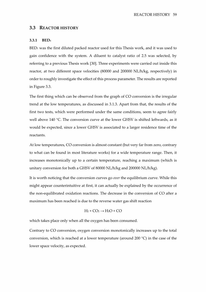
REACTOR HISTORY 59
3.3 REACTOR HISTORY
3.3.1 BED1
BED1 was the first diluted packed reactor used for this Thesis work, and it was used to
gain confidence with the system. A diluent to catalyst ratio of 2.5 was selected, by
referring to a previous Thesis work [30]. Three experiments were carried out inside this
reactor, at two different space velocities (80000 and 200000 NL/h/kg, respectively) in
order to roughly investigate the effect of this process parameter. The results are reported
in Figure 3.3.
The first thing which can be observed from the graph of CO conversion is the irregular
trend at the low temperatures, as discussed in 3.1.3. Apart from that, the results of the
first two tests, which were performed under the same conditions, seem to agree fairly
well above 140 °C. The conversion curve at the lower GHSV is shifted leftwards, as it
would be expected, since a lower GHSV is associated to a larger residence time of the
reactants.
At low temperatures, CO conversion is almost constant (but very far from zero, contrary
to what can be found in most literature works) for a wide temperature range. Then, it
increases monotonically up to a certain temperature, reaching a maximum (which is
unitary conversion for both a GHSV of 80000 NL/h/kg and 200000 NL/h/kg).
It is worth noticing that the conversion curves go over the equilibrium curve. While this
might appear counterintuitive at first, it can actually be explained by the occurrence of
the non-equilibrated oxidation reactions. The decrease in the conversion of CO after a
maximum has been reached is due to the reverse water gas shift reaction
H2 + CO2 → H2O + CO
which takes place only when all the oxygen has been consumed.
Contrary to CO conversion, oxygen conversion monotonically increases up to the total
conversion, which is reached at a lower temperature (around 200 °C) in the case of the
lower space velocity, as expected.
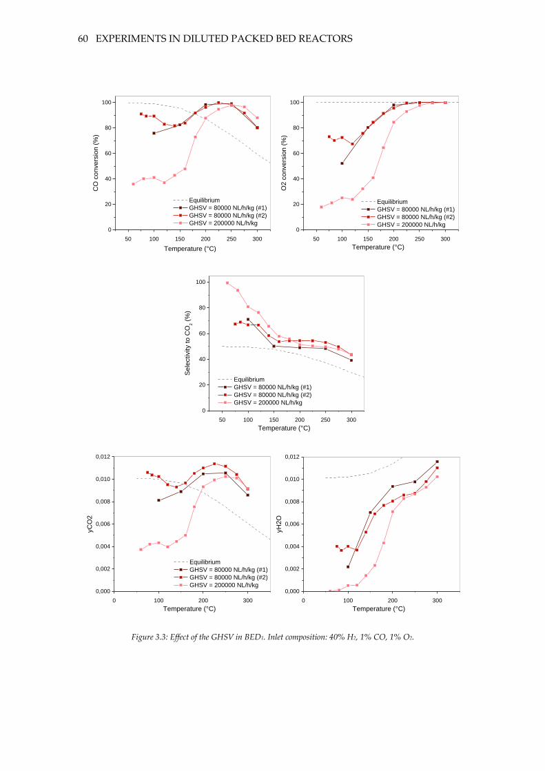
60 EXPERIMENTS IN DILUTED PACKED BED REACTORS
50 100 150 200 250 300
0
20
40
60
80
100
Equilibrium
GHSV = 80000 NL/h/kg (#1)
GHSV = 80000 NL/h/kg (#2)
GHSV = 200000 NL/h/kg
CO
co
nve
rsio
n (
%)
Temperature (°C)
50 100 150 200 250 300
0
20
40
60
80
100
Equilibrium
GHSV = 80000 NL/h/kg (#1)
GHSV = 80000 NL/h/kg (#2)
GHSV = 200000 NL/h/kg
O2 c
on
ve
rsio
n (
%)
Temperature (°C)
50 100 150 200 250 300
0
20
40
60
80
100
Equilibrium
GHSV = 80000 NL/h/kg (#1)
GHSV = 80000 NL/h/kg (#2)
GHSV = 200000 NL/h/kg
Se
lectivity to
CO
2 (
%)
Temperature (°C)
0 100 200 300
0,000
0,002
0,004
0,006
0,008
0,010
0,012
Equilibrium
GHSV = 80000 NL/h/kg (#1)
GHSV = 80000 NL/h/kg (#2)
GHSV = 200000 NL/h/kg
yC
O2
Temperature (°C)
0 100 200 300
0,000
0,002
0,004
0,006
0,008
0,010
0,012
yH
2O
Temperature (°C)
Figure 3.3: Effect of the GHSV in BED1. Inlet composition: 40% H2, 1% CO, 1% O2.
REACTOR HISTORY 61
Oxygen consumption alone is not a very indicative parameter, since it provides no
information about how it is being consumed. Hence, it is worth focusing on the graph of
the selectivity of oxygen to CO. Selectivity is an indicator of how much oxygen is
consumed in the CO oxidation on the basis of the total amount of consumed oxygen. As
previously stated, it is calculated as:
𝑆𝐶𝑂2 =0.5(�̇�𝐶𝑂,𝑖𝑛 − �̇�𝐶𝑂)
�̇�𝑂2,𝑖𝑛 − �̇�𝑂2
Thus, a selectivity lower than the unity indicates that oxygen is being consumed to
produce a species other than carbon dioxide, in this case water. Here, selectivity towards
CO oxidation is monotonically decreasing as the temperature increases, even if the
decrease is significant up to about 150 °C, and weaker at higher temperatures. The
selectivity at low temperatures appears to be significantly higher for a GHSV=200000
NL/h/kg. At higher temperatures, the selectivity remains more or less constant at a value
between 50% and 60%, independently of the space velocity.
yCO2 has the same trend as the conversion of CO. The amount of CO2 is slightly higher
than the one of water until a maximum in the conversion of CO is reached. Surprisingly
enough, CO oxidation seems indeed unaffected by the presence of hydrogen, which is
also competing for oxygen and whose oxidation reaction is known to proceed very fast
towards total conversion even at low temperatures. An explaination for this could be
that CO is saturating the surface of the catalyst, hindering hydrogen oxidation. As the
temperature becomes higher and CO desorption becomes more and more favoured, an
increasing portion of oxygen is consumed in the oxidation of hydrogen.
Contrary to CO2, the amount of water monotonically increases with the temperature.
The yH2O plot reflects the trend of the selectivity, since the presence of water is the direct
indicator of the occurrence of hydrogen oxidation, and thus of the consumption of
oxygen in a reaction other than CO oxidation. It would be very hard to derive any piece
of information starting directly from hydrogen conversion, due to the large experimental
error associated to this parameter. In the case of the lower space velocity, water is
produced even at 60 °C. On the contrary, at the higher space velocity it starts being
produced in meaningful amounts only above 120 °C, meaning that the reaction is still
too slow to be observed at the lower temperatures.
62 EXPERIMENTS IN DILUTED PACKED BED REACTORS
3.3.2 BED2
A deeper investigation on the effect of the GHSV and a study of the effect of oxygen
concentration on the kinetics was carried out in BED2. This reactor is characterized by
the same mass of catalyst as BED1, but a diluent to catalyst ratio (7:1) which is almost
three times and a bed length which is twice (2 cm) the one of the previous bed. The strong
exothermicity of the oxidation reactions was diffucult to deal with inside BED1. By
increasing the mass of inert, the catalyst density in terms of mass of catalyst per unit of
volume of the reactor is reduced, and so are the reaction rate and the rate of heat
production.
The reactor was subjected to the following conditioning procedure in a 40% H2, 60% N2
stream: the temperature was first increased from 30 °C up to 380 °C, at a rate of 3 °C/min.
Then, it was kept at 380 °C for 4 hours and lastly it was cooled down in the reducing
stream up to ambient temperature. Actually, as reported on the product sheet, the
catalyst is said to require no conditioning: however, this was carried out anyway, in
order to check whether it could somehow impact the activity of the catalyst.
Before proceding with the investigation of the effect of GHSV and yO2, a couple of tests
performed under the same operating conditions were carried out in order to verify the
stability of the system: the results agree fairly well. Again, the conversion showed the
previously described decreasing trend injection after injection, going from an initial
value of 23% to a roughly stable value below 10% in 115 minutes (Figure 3.4).
Figure 3.4: Conversion drift in BED2. GHSV=240000 NL/h/kg. Inlet composition: 40% H2, 1% CO, 1% O2.
Injections from 6 up to 15 were carried out around 30 mins after the first five ones, at 10-minute intervals.
0,00
5,00
10,00
15,00
20,00
25,00
0 2 4 6 8 10 12 14 16
X_C
O [
%]
# INJECTION
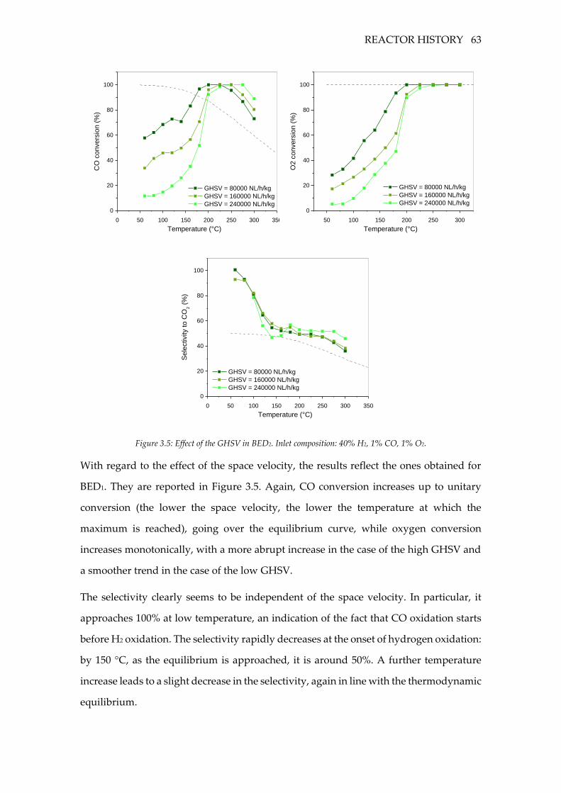
REACTOR HISTORY 63
0 50 100 150 200 250 300 350
0
20
40
60
80
100
GHSV = 80000 NL/h/kg
GHSV = 160000 NL/h/kg
GHSV = 240000 NL/h/kg
CO
co
nve
rsio
n (
%)
Temperature (°C)
50 100 150 200 250 300
0
20
40
60
80
100
GHSV = 80000 NL/h/kg
GHSV = 160000 NL/h/kg
GHSV = 240000 NL/h/kg
O2 c
on
ve
rsio
n (
%)
Temperature (°C)
0 50 100 150 200 250 300 350
0
20
40
60
80
100
GHSV = 80000 NL/h/kg
GHSV = 160000 NL/h/kg
GHSV = 240000 NL/h/kg
Se
lectivity to
CO
2 (
%)
Temperature (°C)
Figure 3.5: Effect of the GHSV in BED2. Inlet composition: 40% H2, 1% CO, 1% O2.
With regard to the effect of the space velocity, the results reflect the ones obtained for
BED1. They are reported in Figure 3.5. Again, CO conversion increases up to unitary
conversion (the lower the space velocity, the lower the temperature at which the
maximum is reached), going over the equilibrium curve, while oxygen conversion
increases monotonically, with a more abrupt increase in the case of the high GHSV and
a smoother trend in the case of the low GHSV.
The selectivity clearly seems to be independent of the space velocity. In particular, it
approaches 100% at low temperature, an indication of the fact that CO oxidation starts
before H2 oxidation. The selectivity rapidly decreases at the onset of hydrogen oxidation:
by 150 °C, as the equilibrium is approached, it is around 50%. A further temperature
increase leads to a slight decrease in the selectivity, again in line with the thermodynamic
equilibrium.
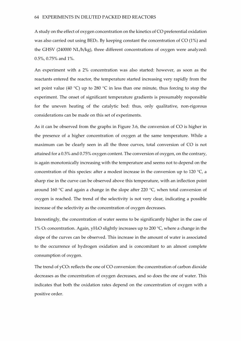
64 EXPERIMENTS IN DILUTED PACKED BED REACTORS
A study on the effect of oxygen concentration on the kinetics of CO preferential oxidation
was also carried out using BED2. By keeping constant the concentration of CO (1%) and
the GHSV (240000 NL/h/kg), three different concentrations of oxygen were analyzed:
0.5%, 0.75% and 1%.
An experiment with a 2% concentration was also started: however, as soon as the
reactants entered the reactor, the temperature started increasing very rapidly from the
set point value (40 °C) up to 280 °C in less than one minute, thus forcing to stop the
experiment. The onset of significant temperature gradients is presumably responsible
for the uneven heating of the catalytic bed: thus, only qualitative, non-rigorous
considerations can be made on this set of experiments.
As it can be observed from the graphs in Figure 3.6, the conversion of CO is higher in
the presence of a higher concentration of oxygen at the same temperature. While a
maximum can be clearly seen in all the three curves, total conversion of CO is not
attained for a 0.5% and 0.75% oxygen content. The conversion of oxygen, on the contrary,
is again monotonically increasing with the temperature and seems not to depend on the
concentration of this species: after a modest increase in the conversion up to 120 °C, a
sharp rise in the curve can be observed above this temperature, with an inflection point
around 160 °C and again a change in the slope after 220 °C, when total conversion of
oxygen is reached. The trend of the selectivity is not very clear, indicating a possible
increase of the selectivity as the concentration of oxygen decreases.
Interestingly, the concentration of water seems to be significantly higher in the case of
1% O2 concentration. Again, yH2O slightly increases up to 200 °C, where a change in the
slope of the curves can be observed. This increase in the amount of water is associated
to the occurrence of hydrogen oxidation and is concomitant to an almost complete
consumption of oxygen.
The trend of yCO2 reflects the one of CO conversion: the concentration of carbon dioxide
decreases as the concentration of oxygen decreases, and so does the one of water. This
indicates that both the oxidation rates depend on the concentration of oxygen with a
positive order.
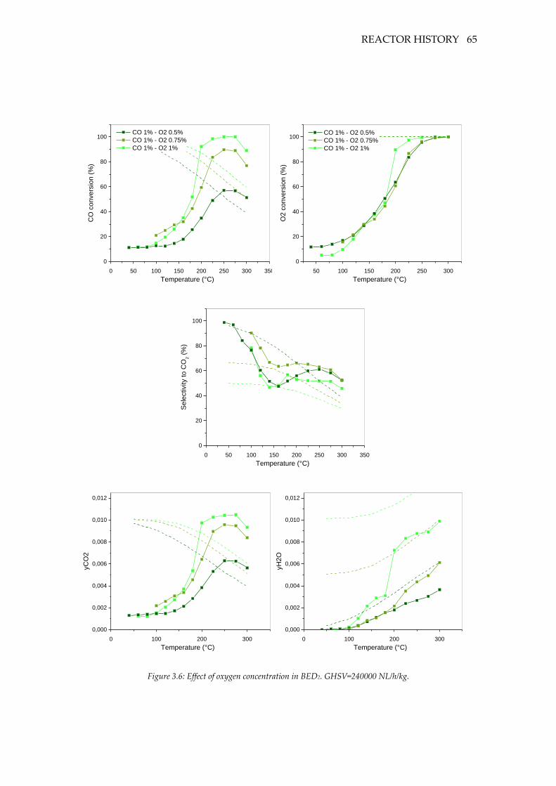
REACTOR HISTORY 65
0 50 100 150 200 250 300 350
0
20
40
60
80
100 CO 1% - O2 0.5%
CO 1% - O2 0.75%
CO 1% - O2 1%
CO
co
nve
rsio
n (
%)
Temperature (°C)
50 100 150 200 250 300
0
20
40
60
80
100 CO 1% - O2 0.5%
CO 1% - O2 0.75%
CO 1% - O2 1%
O2 c
on
ve
rsio
n (
%)
Temperature (°C)
0 50 100 150 200 250 300 350
0
20
40
60
80
100
Se
lectivity to
CO
2 (
%)
Temperature (°C)
0 100 200 300
0,000
0,002
0,004
0,006
0,008
0,010
0,012
yC
O2
Temperature (°C)
0 100 200 300
0,000
0,002
0,004
0,006
0,008
0,010
0,012
yH
2O
Temperature (°C)
Figure 3.6: Effect of oxygen concentration in BED2. GHSV=240000 NL/h/kg.
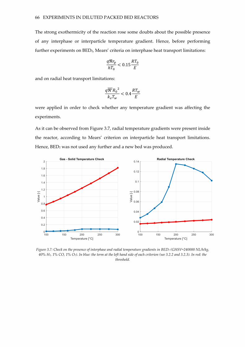
66 EXPERIMENTS IN DILUTED PACKED BED REACTORS
The strong exothermicity of the reaction rose some doubts about the possible presence
of any interphase or interparticle temperature gradient. Hence, before performing
further experiments on BED2, Mears’ criteria on interphase heat transport limitations:
𝑞ℜ𝑟𝑝
ℎ𝑇0< 0.15
𝑅𝑇0𝐸
and on radial heat transport limitations:
𝑞ℜ′̅̅ ̅𝑅02
𝑘𝑒𝑇𝑤< 0.4
𝑅𝑇𝑤𝐸
were applied in order to check whether any temperature gradient was affecting the
experiments.
As it can be observed from Figure 3.7, radial temperature gradients were present inside
the reactor, according to Mears’ criterion on interparticle heat transport limitations.
Hence, BED2 was not used any further and a new bed was produced.
Figure 3.7: Check on the presence of interphase and radial temperature gradients in BED2 (GHSV=240000 NL/h/kg,
40% H2, 1% CO, 1% O2). In blue: the term at the left hand side of each criterion (see 3.2.2 and 3.2.3). In red: the
threshold.
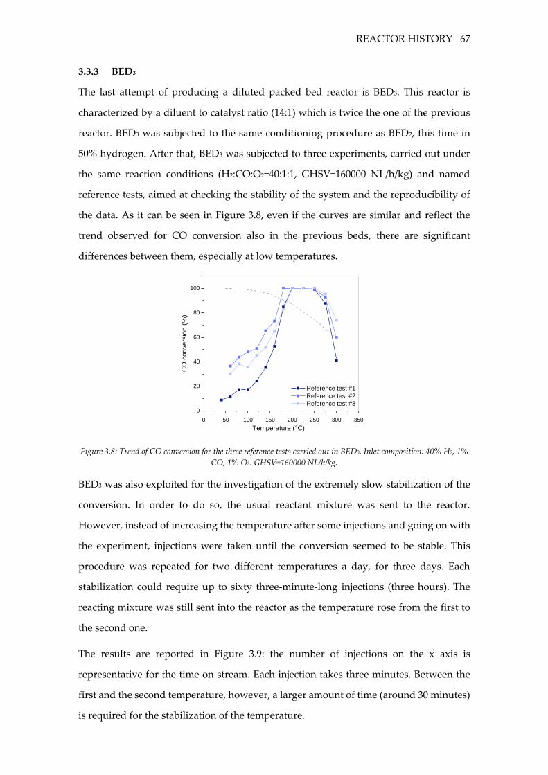
REACTOR HISTORY 67
3.3.3 BED3
The last attempt of producing a diluted packed bed reactor is BED3. This reactor is
characterized by a diluent to catalyst ratio (14:1) which is twice the one of the previous
reactor. BED3 was subjected to the same conditioning procedure as BED2, this time in
50% hydrogen. After that, BED3 was subjected to three experiments, carried out under
the same reaction conditions (H2:CO:O2=40:1:1, GHSV=160000 NL/h/kg) and named
reference tests, aimed at checking the stability of the system and the reproducibility of
the data. As it can be seen in Figure 3.8, even if the curves are similar and reflect the
trend observed for CO conversion also in the previous beds, there are significant
differences between them, especially at low temperatures.
0 50 100 150 200 250 300 350
0
20
40
60
80
100
Reference test #1
Reference test #2
Reference test #3
CO
convers
ion (
%)
Temperature (°C)
Figure 3.8: Trend of CO conversion for the three reference tests carried out in BED3. Inlet composition: 40% H2, 1%
CO, 1% O2. GHSV=160000 NL/h/kg.
BED3 was also exploited for the investigation of the extremely slow stabilization of the
conversion. In order to do so, the usual reactant mixture was sent to the reactor.
However, instead of increasing the temperature after some injections and going on with
the experiment, injections were taken until the conversion seemed to be stable. This
procedure was repeated for two different temperatures a day, for three days. Each
stabilization could require up to sixty three-minute-long injections (three hours). The
reacting mixture was still sent into the reactor as the temperature rose from the first to
the second one.
The results are reported in Figure 3.9: the number of injections on the x axis is
representative for the time on stream. Each injection takes three minutes. Between the
first and the second temperature, however, a larger amount of time (around 30 minutes)
is required for the stabilization of the temperature.
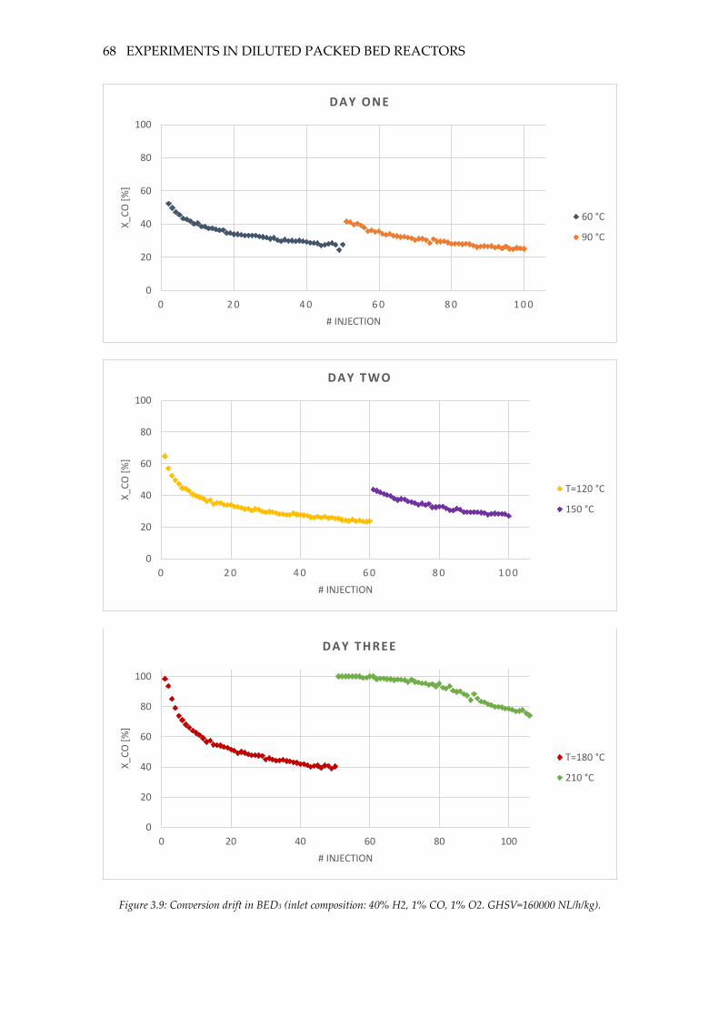
68 EXPERIMENTS IN DILUTED PACKED BED REACTORS
Figure 3.9: Conversion drift in BED3 (inlet composition: 40% H2, 1% CO, 1% O2. GHSV=160000 NL/h/kg).
0
20
40
60
80
100
0 2 0 4 0 6 0 8 0 1 0 0
X_C
O [
%]
# INJECTION
DAY ONE
60 °C
90 °C
0
20
40
60
80
100
0 2 0 4 0 6 0 8 0 1 0 0
X_C
O [
%]
# INJECTION
DAY TWO
T=120 °C
150 °C
0
20
40
60
80
100
0 20 40 60 80 100
X_C
O [
%]
# INJECTION
DAY THREE
T=180 °C
210 °C
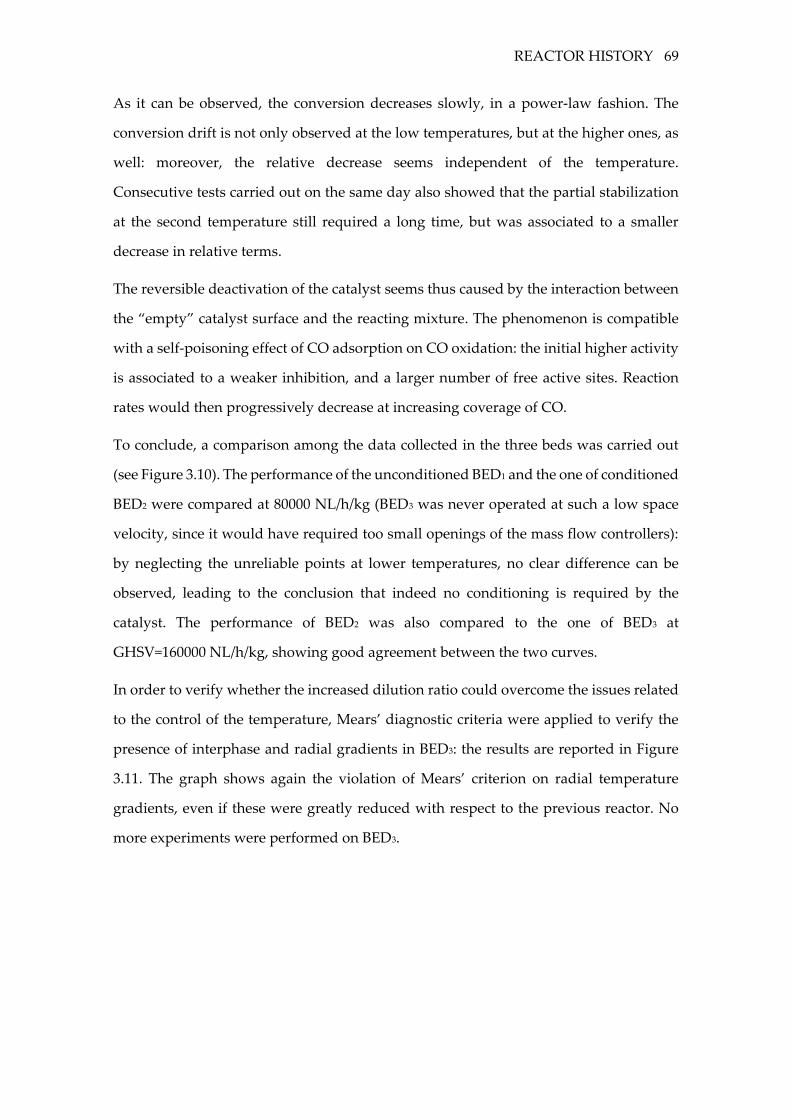
REACTOR HISTORY 69
As it can be observed, the conversion decreases slowly, in a power-law fashion. The
conversion drift is not only observed at the low temperatures, but at the higher ones, as
well: moreover, the relative decrease seems independent of the temperature.
Consecutive tests carried out on the same day also showed that the partial stabilization
at the second temperature still required a long time, but was associated to a smaller
decrease in relative terms.
The reversible deactivation of the catalyst seems thus caused by the interaction between
the “empty” catalyst surface and the reacting mixture. The phenomenon is compatible
with a self-poisoning effect of CO adsorption on CO oxidation: the initial higher activity
is associated to a weaker inhibition, and a larger number of free active sites. Reaction
rates would then progressively decrease at increasing coverage of CO.
To conclude, a comparison among the data collected in the three beds was carried out
(see Figure 3.10). The performance of the unconditioned BED1 and the one of conditioned
BED2 were compared at 80000 NL/h/kg (BED3 was never operated at such a low space
velocity, since it would have required too small openings of the mass flow controllers):
by neglecting the unreliable points at lower temperatures, no clear difference can be
observed, leading to the conclusion that indeed no conditioning is required by the
catalyst. The performance of BED2 was also compared to the one of BED3 at
GHSV=160000 NL/h/kg, showing good agreement between the two curves.
In order to verify whether the increased dilution ratio could overcome the issues related
to the control of the temperature, Mears’ diagnostic criteria were applied to verify the
presence of interphase and radial gradients in BED3: the results are reported in Figure
3.11. The graph shows again the violation of Mears’ criterion on radial temperature
gradients, even if these were greatly reduced with respect to the previous reactor. No
more experiments were performed on BED3.
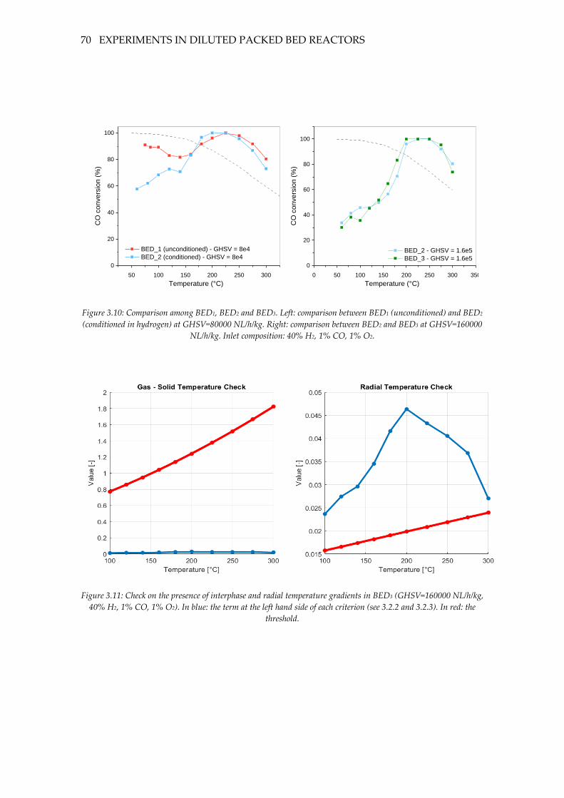
70 EXPERIMENTS IN DILUTED PACKED BED REACTORS
50 100 150 200 250 300
0
20
40
60
80
100
BED_1 (unconditioned) - GHSV = 8e4
BED_2 (conditioned) - GHSV = 8e4
CO
co
nve
rsio
n (
%)
Temperature (°C)
0 50 100 150 200 250 300 350
0
20
40
60
80
100
BED_2 - GHSV = 1.6e5
BED_3 - GHSV = 1.6e5
CO
co
nve
rsio
n (
%)
Temperature (°C)
Figure 3.10: Comparison among BED1, BED2 and BED3. Left: comparison between BED1 (unconditioned) and BED2
(conditioned in hydrogen) at GHSV=80000 NL/h/kg. Right: comparison between BED2 and BED3 at GHSV=160000
NL/h/kg. Inlet composition: 40% H2, 1% CO, 1% O2.
Figure 3.11: Check on the presence of interphase and radial temperature gradients in BED3 (GHSV=160000 NL/h/kg,
40% H2, 1% CO, 1% O2). In blue: the term at the left hand side of each criterion (see 3.2.2 and 3.2.3). In red: the
threshold.

REACTOR HISTORY 71
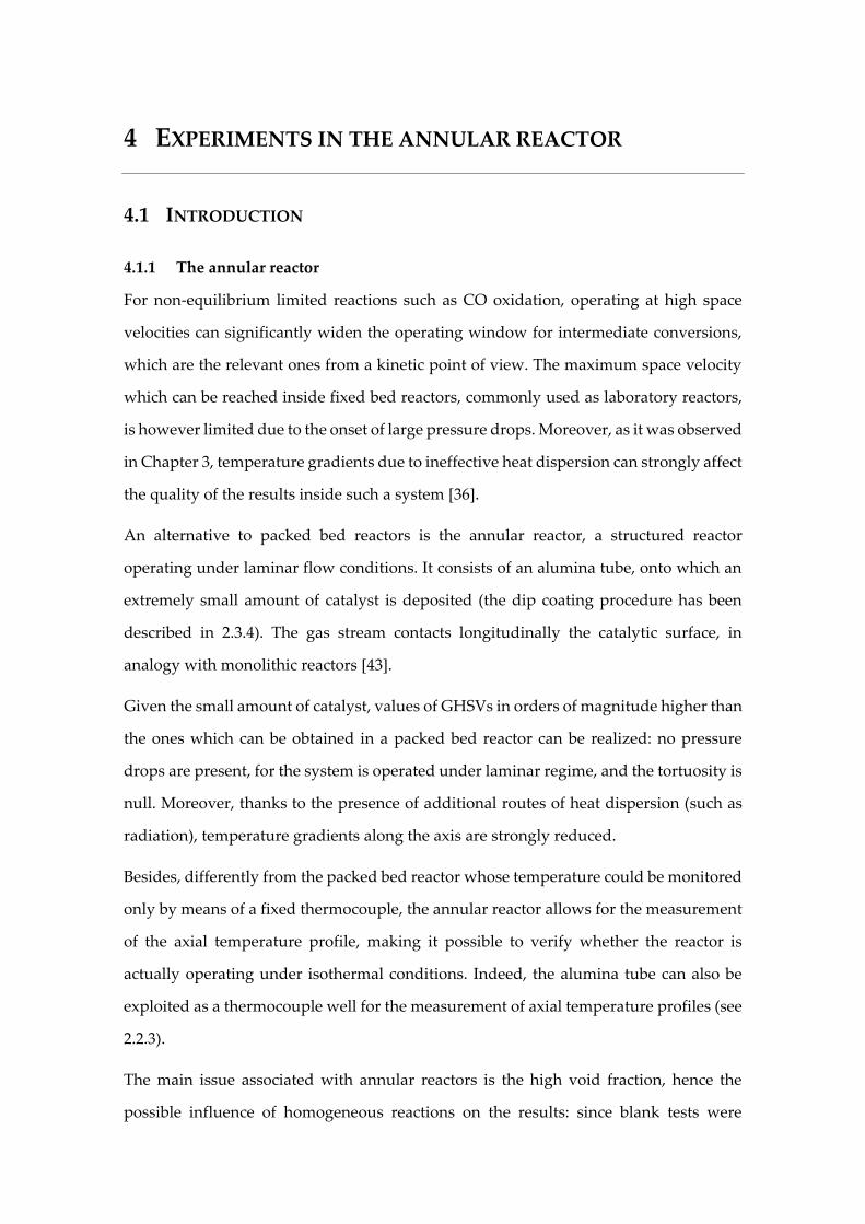
4 EXPERIMENTS IN THE ANNULAR REACTOR
4.1 INTRODUCTION
4.1.1 The annular reactor
For non-equilibrium limited reactions such as CO oxidation, operating at high space
velocities can significantly widen the operating window for intermediate conversions,
which are the relevant ones from a kinetic point of view. The maximum space velocity
which can be reached inside fixed bed reactors, commonly used as laboratory reactors,
is however limited due to the onset of large pressure drops. Moreover, as it was observed
in Chapter 3, temperature gradients due to ineffective heat dispersion can strongly affect
the quality of the results inside such a system [36].
An alternative to packed bed reactors is the annular reactor, a structured reactor
operating under laminar flow conditions. It consists of an alumina tube, onto which an
extremely small amount of catalyst is deposited (the dip coating procedure has been
described in 2.3.4). The gas stream contacts longitudinally the catalytic surface, in
analogy with monolithic reactors [43].
Given the small amount of catalyst, values of GHSVs in orders of magnitude higher than
the ones which can be obtained in a packed bed reactor can be realized: no pressure
drops are present, for the system is operated under laminar regime, and the tortuosity is
null. Moreover, thanks to the presence of additional routes of heat dispersion (such as
radiation), temperature gradients along the axis are strongly reduced.
Besides, differently from the packed bed reactor whose temperature could be monitored
only by means of a fixed thermocouple, the annular reactor allows for the measurement
of the axial temperature profile, making it possible to verify whether the reactor is
actually operating under isothermal conditions. Indeed, the alumina tube can also be
exploited as a thermocouple well for the measurement of axial temperature profiles (see
2.2.3).
The main issue associated with annular reactors is the high void fraction, hence the
possible influence of homogeneous reactions on the results: since blank tests were
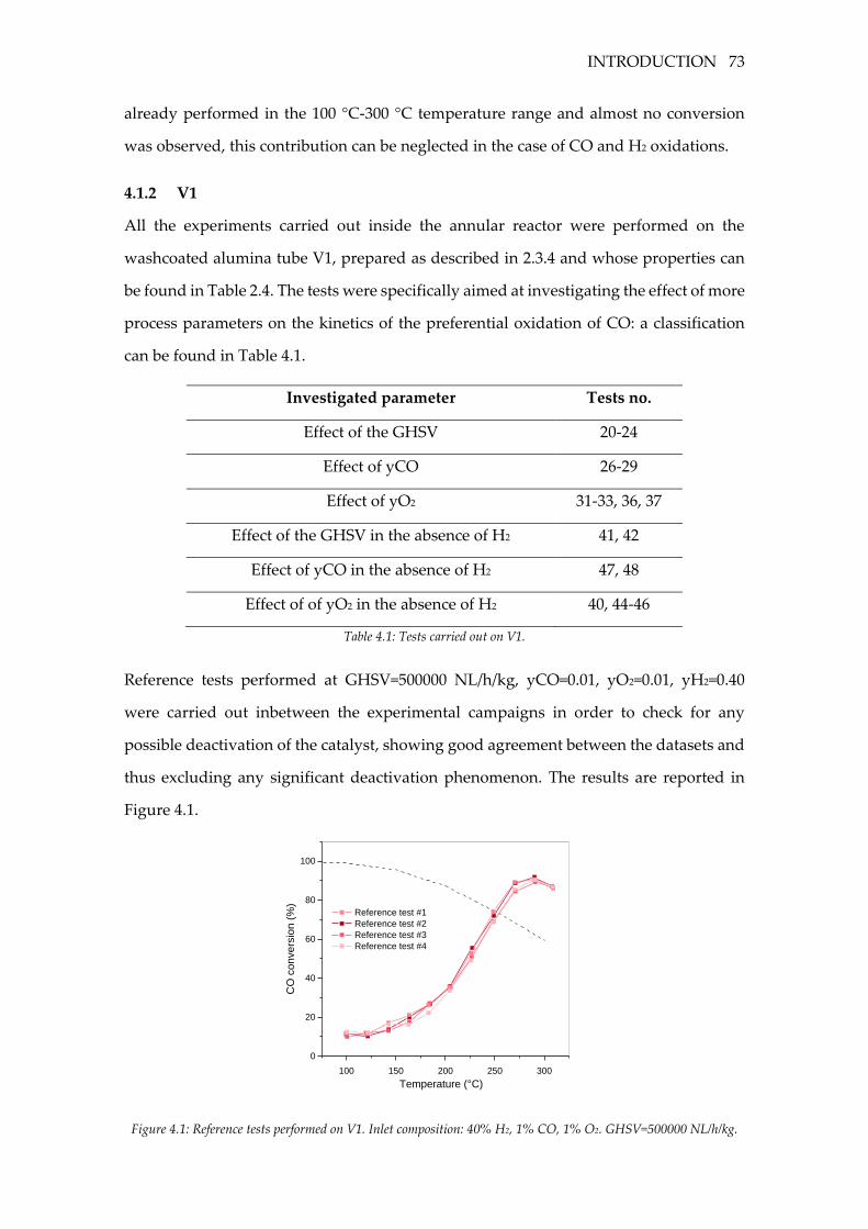
INTRODUCTION 73
already performed in the 100 °C-300 °C temperature range and almost no conversion
was observed, this contribution can be neglected in the case of CO and H2 oxidations.
4.1.2 V1
All the experiments carried out inside the annular reactor were performed on the
washcoated alumina tube V1, prepared as described in 2.3.4 and whose properties can
be found in Table 2.4. The tests were specifically aimed at investigating the effect of more
process parameters on the kinetics of the preferential oxidation of CO: a classification
can be found in Table 4.1.
Investigated parameter Tests no.
Effect of the GHSV 20-24
Effect of yCO 26-29
Effect of yO2 31-33, 36, 37
Effect of the GHSV in the absence of H2 41, 42
Effect of yCO in the absence of H2 47, 48
Effect of of yO2 in the absence of H2 40, 44-46
Table 4.1: Tests carried out on V1.
Reference tests performed at GHSV=500000 NL/h/kg, yCO=0.01, yO2=0.01, yH2=0.40
were carried out inbetween the experimental campaigns in order to check for any
possible deactivation of the catalyst, showing good agreement between the datasets and
thus excluding any significant deactivation phenomenon. The results are reported in
Figure 4.1.
100 150 200 250 300
0
20
40
60
80
100
Reference test #1
Reference test #2
Reference test #3
Reference test #4
CO
co
nve
rsio
n (
%)
Temperature (°C)
Figure 4.1: Reference tests performed on V1. Inlet composition: 40% H2, 1% CO, 1% O2. GHSV=500000 NL/h/kg.
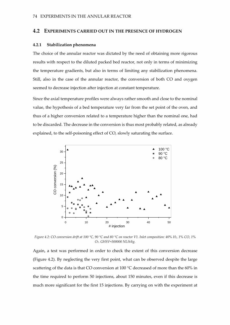
74 EXPERIMENTS IN THE ANNULAR REACTOR
4.2 EXPERIMENTS CARRIED OUT IN THE PRESENCE OF HYDROGEN
4.2.1 Stabilization phenomena
The choice of the annular reactor was dictated by the need of obtaining more rigorous
results with respect to the diluted packed bed reactor, not only in terms of minimizing
the temperature gradients, but also in terms of limiting any stabilization phenomena.
Still, also in the case of the annular reactor, the conversion of both CO and oxygen
seemed to decrease injection after injection at constant temperature.
Since the axial temperature profiles were always rather smooth and close to the nominal
value, the hypothesis of a bed temperature very far from the set point of the oven, and
thus of a higher conversion related to a temperature higher than the nominal one, had
to be discarded. The decrease in the conversion is thus most probably related, as already
explained, to the self-poisoning effect of CO, slowly saturating the surface.
0 10 20 30 40 50
0
5
10
15
20
25
30 100 °C
90 °C
80 °C
CO
co
nve
rsio
n (
%)
# injection
Figure 4.2: CO conversion drift at 100 °C, 90 °C and 80 °C on reactor V1. Inlet composition: 40% H2, 1% CO, 1%
O2. GHSV=500000 NL/h/kg.
Again, a test was performed in order to check the extent of this conversion decrease
(Figure 4.2). By neglecting the very first point, what can be observed despite the large
scattering of the data is that CO conversion at 100 °C decreased of more than the 60% in
the time required to perform 50 injections, about 150 minutes, even if this decrease is
much more significant for the first 15 injections. By carrying on with the experiment at
EXPERIMENTS CARRIED OUT IN THE PRESENCE OF HYDROGEN 75
90 °C and 80 °C, a further decrease in the conversion injection after injection could be
observed. The whole test took around 6 hours.
Since the phenomenon could not be limited, being it related to the reaction mechanism
itself, and since obtaining a stable system should have required an amount of time
significantly longer than the time to complete the tests themselves, it was chosen not to
wait for the complete stabilization, and to continue performing the experiments under
unsteady conditions. However, a partial stabilization was obtained at the beginning of
each experiment by waiting at least 30 minutes for measuring the concentration of the
products. By carrying out the same standardized procedure at every experiment, a good
reproducibility of the results was achieved and the three injections taken at each
temperature seemed not to follow any systematic trend.
Figure 4.3: Trend of the outlet flow rate of CO for the three injections taken at each temperature. GHSV=500000
NL/h/kg. Inlet concentration: 40% H2, 1% CO, 1% O2.
Data measured at the lower temperatures were anyway not considered for the
quantitative kinetic study. Indeed, they are those affected by the highest uncertainty,
both due to the fact that they were gathered after a short time on stream, and also since
CO desorption, possibly limiting the self-poisoning effect, is favoured only at higher
temperatures.
0
0,2
0,4
0,6
0,8
1
1,2
0 1 2 3 4
F_C
O_o
ut
[Nm
L/m
in]
# injection
100 °C
120 °C
140 °C
160 °C
180 °C
200 °C
220 °C
240 °C
260 °C
280 °C
300 °C
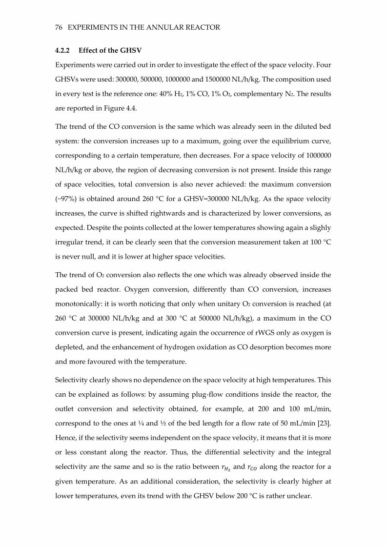
76 EXPERIMENTS IN THE ANNULAR REACTOR
4.2.2 Effect of the GHSV
Experiments were carried out in order to investigate the effect of the space velocity. Four
GHSVs were used: 300000, 500000, 1000000 and 1500000 NL/h/kg. The composition used
in every test is the reference one: 40% H2, 1% CO, 1% O2, complementary N2. The results
are reported in Figure 4.4.
The trend of the CO conversion is the same which was already seen in the diluted bed
system: the conversion increases up to a maximum, going over the equilibrium curve,
corresponding to a certain temperature, then decreases. For a space velocity of 1000000
NL/h/kg or above, the region of decreasing conversion is not present. Inside this range
of space velocities, total conversion is also never achieved: the maximum conversion
(~97%) is obtained around 260 °C for a GHSV=300000 NL/h/kg. As the space velocity
increases, the curve is shifted rightwards and is characterized by lower conversions, as
expected. Despite the points collected at the lower temperatures showing again a slighly
irregular trend, it can be clearly seen that the conversion measurement taken at 100 °C
is never null, and it is lower at higher space velocities.
The trend of O2 conversion also reflects the one which was already observed inside the
packed bed reactor. Oxygen conversion, differently than CO conversion, increases
monotonically: it is worth noticing that only when unitary O2 conversion is reached (at
260 °C at 300000 NL/h/kg and at 300 °C at 500000 NL/h/kg), a maximum in the CO
conversion curve is present, indicating again the occurrence of rWGS only as oxygen is
depleted, and the enhancement of hydrogen oxidation as CO desorption becomes more
and more favoured with the temperature.
Selectivity clearly shows no dependence on the space velocity at high temperatures. This
can be explained as follows: by assuming plug-flow conditions inside the reactor, the
outlet conversion and selectivity obtained, for example, at 200 and 100 mL/min,
correspond to the ones at ¼ and ½ of the bed length for a flow rate of 50 mL/min [23].
Hence, if the selectivity seems independent on the space velocity, it means that it is more
or less constant along the reactor. Thus, the differential selectivity and the integral
selectivity are the same and so is the ratio between 𝑟𝐻2 and 𝑟𝐶𝑂 along the reactor for a
given temperature. As an additional consideration, the selectivity is clearly higher at
lower temperatures, even its trend with the GHSV below 200 °C is rather unclear.
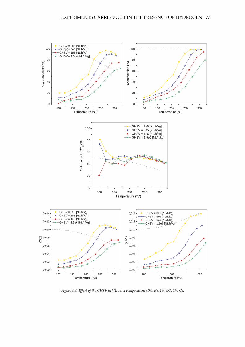
EXPERIMENTS CARRIED OUT IN THE PRESENCE OF HYDROGEN 77
100 150 200 250 300
0
20
40
60
80
100 GHSV = 3e5 [NL/h/kg]
GHSV = 5e5 [NL/h/kg]
GHSV = 1e6 [NL/h/kg]
GHSV = 1.5e6 [NL/h/kg]
CO
co
nve
rsio
n (
%)
Temperature (°C)
100 150 200 250 300
0
20
40
60
80
100
O2 c
on
ve
rsio
n (
%)
Temperature (°C)
100 150 200 250 300
0
20
40
60
80
100 GHSV = 3e5 [NL/h/kg]
GHSV = 5e5 [NL/h/kg]
GHSV = 1e6 [NL/h/kg]
GHSV = 1.5e6 [NL/h/kg]
Se
lectivity to
CO
2 (
%)
Temperature (°C)
100 150 200 250 300
0,000
0,002
0,004
0,006
0,008
0,010
0,012
0,014 GHSV = 3e5 [NL/h/kg]
GHSV = 5e5 [NL/h/kg]
GHSV = 1e6 [NL/h/kg]
GHSV = 1.5e6 [NL/h/kg]
yC
O2
Temperature (°C)
100 200 300
0,000
0,002
0,004
0,006
0,008
0,010
0,012
0,014 GHSV = 3e5 [NL/h/kg]
GHSV = 5e5 [NL/h/kg]
GHSV = 1e6 [NL/h/kg]
GHSV = 1.5e6 [NL/h/kg]
yH
2O
Temperature (°C)
Figure 4.4: Effect of the GHSV in V1. Inlet composition: 40% H2, 1% CO, 1% O2.
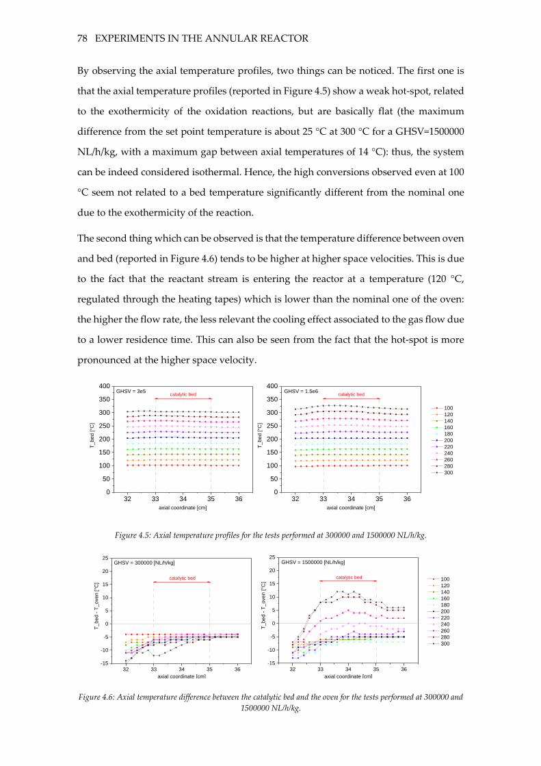
78 EXPERIMENTS IN THE ANNULAR REACTOR
By observing the axial temperature profiles, two things can be noticed. The first one is
that the axial temperature profiles (reported in Figure 4.5) show a weak hot-spot, related
to the exothermicity of the oxidation reactions, but are basically flat (the maximum
difference from the set point temperature is about 25 °C at 300 °C for a GHSV=1500000
NL/h/kg, with a maximum gap between axial temperatures of 14 °C): thus, the system
can be indeed considered isothermal. Hence, the high conversions observed even at 100
°C seem not related to a bed temperature significantly different from the nominal one
due to the exothermicity of the reaction.
The second thing which can be observed is that the temperature difference between oven
and bed (reported in Figure 4.6) tends to be higher at higher space velocities. This is due
to the fact that the reactant stream is entering the reactor at a temperature (120 °C,
regulated through the heating tapes) which is lower than the nominal one of the oven:
the higher the flow rate, the less relevant the cooling effect associated to the gas flow due
to a lower residence time. This can also be seen from the fact that the hot-spot is more
pronounced at the higher space velocity.
32 33 34 35 360
50
100
150
200
250
300
350
400GHSV = 3e5
T_
be
d [
°C]
axial coordinate [cm]
catalytic bed
100
120
140
160
180
200
220
240
260
280
300
32 33 34 35 360
50
100
150
200
250
300
350
400GHSV = 1.5e6
T_
be
d [
°C]
axial coordinate [cm]
catalytic bed
100
120
140
160
180
200
220
240
260
280
300
Figure 4.5: Axial temperature profiles for the tests performed at 300000 and 1500000 NL/h/kg.
32 33 34 35 36-15
-10
-5
0
5
10
15
20
25GHSV = 300000 [NL/h/kg]
100
120
140
160
180
200
220
240
260
280
300
T_bed -
T_oven [°C
]
axial coordinate [cm]
catalytic bed
32 33 34 35 36-15
-10
-5
0
5
10
15
20
25GHSV = 1500000 [NL/h/kg]
100
120
140
160
180
200
220
240
260
280
300
T_
be
d -
T_
ove
n [
°C]
axial coordinate [cm]
catalytic bed
Figure 4.6: Axial temperature difference between the catalytic bed and the oven for the tests performed at 300000 and
1500000 NL/h/kg.
EXPERIMENTS CARRIED OUT IN THE PRESENCE OF HYDROGEN 79
4.2.3 Effect of yCO
The effect of the concentration of carbon monoxide on the kinetics of CO PrOx was
investigated by performing a series of tests at different CO concentration, ranging from
0.5% up to 4%: the results are reported in Figure 4.7. Oxygen concentration is 1% and the
GHSV is 500000 NL/h/kg for all tests. This study was not carried out inside the diluted
packed bed reactor.
CO conversion clearly increases as its concentration decreases, at least up to 200 °C,
when a change in the trend of the curves at lower concentration of CO can be observed.
In fact, while in the case of a 0.5% and 1% concentration a maximum is present at 220 °C
and 280 °C, respectively, the curves obtained for yCO=4% and yCO=2% are only
monotonically increasing up to 300 °C. Total CO conversion is never achieved: the
maximum conversion (around 97%) is obtained for a CO concentration of 0.5%. The
effect of CO concentration on the conversion is indicative of a reaction order significantly
lower than 1.
Oxygen conversion monotonically increases with the temperature in every test, but
shows a progressive decrease at increasing CO concentration. It is worth noticing that,
for a 2% and a 4% CO concentration, total O2 conversion is not reached at 300 °C.
The amount of CO2, the product of CO oxidation, follows the same trend as CO
conversion. Its production slightly decreases at increasing CO concentration: the effect
is more important at intermediate temperatures (180-200 °C). At higher temperatures,
the presence of the stoichiometric constraint causes a flattening in the trend of the
concentration. The curves have a tendency to overlap, especially at lower temperatures,
despite yCO2 being slightly higher in the case of lower CO concentrations: hence, it can
be concluded that the reaction rate most probably depends on CO concentration with a
negative reaction order, which seems however close to 0.
The amount of water seems insensitive to the concentration of CO, at least above a 1%
CO concentration. However, the amount of water produced for hydrogen oxidation is
remarkably higher for the lowest CO concentration (0.5%), even at the lower
temperatures: a sharp increase in water concentration can be observed between 180 °C
and 200°C, as oxygen is depleted.
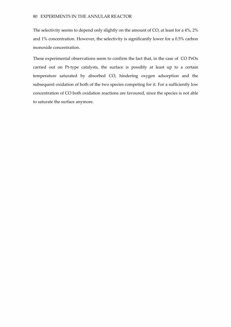
80 EXPERIMENTS IN THE ANNULAR REACTOR
The selectivity seems to depend only slightly on the amount of CO, at least for a 4%, 2%
and 1% concentration. However, the selectivity is significantly lower for a 0.5% carbon
monoxide concentration.
These experimental observations seem to confirm the fact that, in the case of CO PrOx
carried out on Pt-type catalysts, the surface is possibly at least up to a certain
temperature saturated by absorbed CO, hindering oxygen adsorption and the
subsequent oxidation of both of the two species competing for it. For a sufficiently low
concentration of CO both oxidation reactions are favoured, since the species is not able
to saturate the surface anymore.
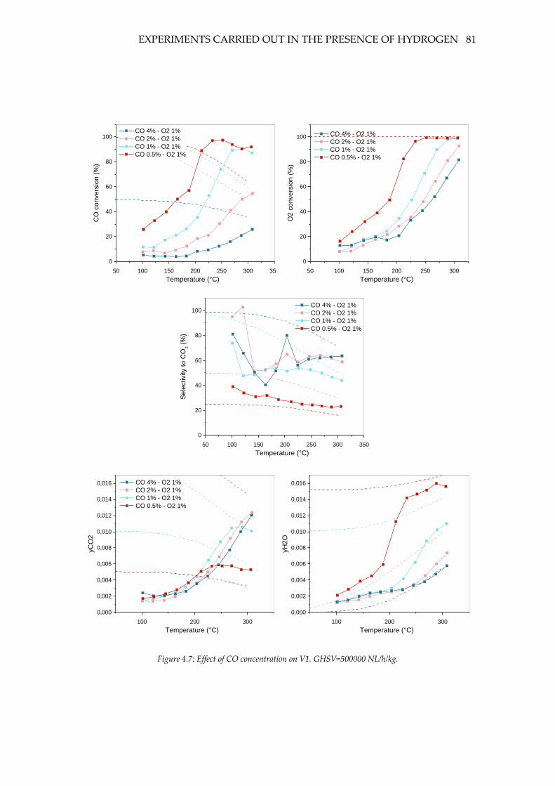
EXPERIMENTS CARRIED OUT IN THE PRESENCE OF HYDROGEN 81
50 100 150 200 250 300 350
0
20
40
60
80
100 CO 4% - O2 1%
CO 2% - O2 1%
CO 1% - O2 1%
CO 0.5% - O2 1%
CO
co
nve
rsio
n (
%)
Temperature (°C)
50 100 150 200 250 300
0
20
40
60
80
100 CO 4% - O2 1%
CO 2% - O2 1%
CO 1% - O2 1%
CO 0.5% - O2 1%
O2 c
on
ve
rsio
n (
%)
Temperature (°C)
50 100 150 200 250 300 350
0
20
40
60
80
100 CO 4% - O2 1%
CO 2% - O2 1%
CO 1% - O2 1%
CO 0.5% - O2 1%
Sele
ctivity to C
O2 (
%)
Temperature (°C)
100 200 300
0,000
0,002
0,004
0,006
0,008
0,010
0,012
0,014
0,016 CO 4% - O2 1%
CO 2% - O2 1%
CO 1% - O2 1%
CO 0.5% - O2 1%
yC
O2
Temperature (°C)
100 200 300
0,000
0,002
0,004
0,006
0,008
0,010
0,012
0,014
0,016
yH
2O
Temperature (°C)
Figure 4.7: Effect of CO concentration on V1. GHSV=500000 NL/h/kg.
82 EXPERIMENTS IN THE ANNULAR REACTOR
4.2.4 Effect of yO2
In order to study the effect of the concentration of oxygen on the kinetics of CO, a series
of test at different O2 amount were carried out. In particular, yO2 was varied between
0.25% and 4% while CO concentration was always equal to 1% and the GHSV to 500000
NL/h/kg. The results are reported in Figure 4.8.
The results are in good agreement with the ones obtained for the diluted packed bed.
CO conversion clearly depends on oxygen concentration. In particular, higher oxygen
concentrations correspond to higher conversions. The conversion is significantly smaller
at lower temperatures, possibly due to the large CO surface coverage.
Oxygen conversion decreases moderately at increasing oxygen concentration below 175
°C, suggesting a reaction order lower than 1 for this temperature range. On the contrary,
above 175 °C, the conversion of O2 increases as its concentration increases, possibly due
to the larger conversion of CO.
The selectivity seems to be more or less constant and decreasing as T increases for a wide
range of O2 concentrations. However, for a 2% and 4% oxygen concentration, the
selectivity is significantly lower, and the concentration of water produced in hydrogen
oxidation is much higher. Hence, a oxygen concentration significantly higher than the
stoichiometric value seems to be detrimental for the selectivity, even at the low
temperatures.
The amount of both CO2 and H2O is higher at higher oxygen concentration. This is an
indication of a positive order kinetics, possibly first order since the concentration of the
products is increasing more or less linearly (apart from the test at 4% O2 concentration)
with oxygen concentration at the lower temperatures.
EXPERIMENTS CARRIED OUT IN THE PRESENCE OF HYDROGEN 83
100 150 200 250 300
0
20
40
60
80
100
O2 4%
O2 2%
O2 1%
O2 0.75%
O2 0.5%
O2 0.25%
CO
co
nve
rsio
n (
%)
Temperature (°C)
100 150 200 250 300
0
20
40
60
80
100 O2 4%
O2 2%
O2 1%
O2 0.75%
O2 0.5%
O2 0.25%
O2 c
on
ve
rsio
n (
%)
Temperature (°C)
50 100 150 200 250 300 350
0
20
40
60
80
100
Se
lectivity to
CO
2 (
%)
Temperature (°C)
50 100 150 200 250 300 350
0,000
0,002
0,004
0,006
0,008
0,010
0,012 O2 4%
O2 2%
O2 1%
O2 0.75%
O2 0.5%
O2 0.25%
yC
O2
Temperature (°C)
50 100 150 200 250 300 350
0,00
0,01
0,02
0,03
0,04
0,05
0,06
0,07
0,08
0,09
0,10
yH
2O
Temperature (°C)
Figure 4.8: Effect of oxygen concentration on V1. GHSV=500000 NL/h/kg.
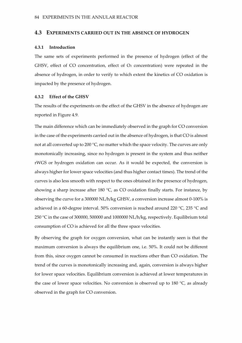
84 EXPERIMENTS IN THE ANNULAR REACTOR
4.3 EXPERIMENTS CARRIED OUT IN THE ABSENCE OF HYDROGEN
4.3.1 Introduction
The same sets of experiments performed in the presence of hydrogen (effect of the
GHSV, effect of CO concentration, effect of O2 concentration) were repeated in the
absence of hydrogen, in order to verify to which extent the kinetics of CO oxidation is
impacted by the presence of hydrogen.
4.3.2 Effect of the GHSV
The results of the experiments on the effect of the GHSV in the absence of hydrogen are
reported in Figure 4.9.
The main difference which can be immediately observed in the graph for CO conversion
in the case of the experiments carried out in the absence of hydrogen, is that CO is almost
not at all converted up to 200 °C, no matter which the space velocity. The curves are only
monotonically increasing, since no hydrogen is present in the system and thus neither
rWGS or hydrogen oxidation can occur. As it would be expected, the conversion is
always higher for lower space velocities (and thus higher contact times). The trend of the
curves is also less smooth with respect to the ones obtained in the presence of hydrogen,
showing a sharp increase after 180 °C, as CO oxidation finally starts. For instance, by
observing the curve for a 300000 NL/h/kg GHSV, a conversion increase almost 0-100% is
achieved in a 60-degree interval. 50% conversion is reached around 220 °C, 235 °C and
250 °C in the case of 300000, 500000 and 1000000 NL/h/kg, respectively. Equilibrium total
consumption of CO is achieved for all the three space velocities.
By observing the graph for oxygen conversion, what can be instantly seen is that the
maximum conversion is always the equilibrium one, i.e. 50%. It could not be different
from this, since oxygen cannot be consumed in reactions other than CO oxidation. The
trend of the curves is monotonically increasing and, again, conversion is always higher
for lower space velocities. Equilibrium conversion is achieved at lower temperatures in
the case of lower space velocities. No conversion is observed up to 180 °C, as already
observed in the graph for CO conversion.
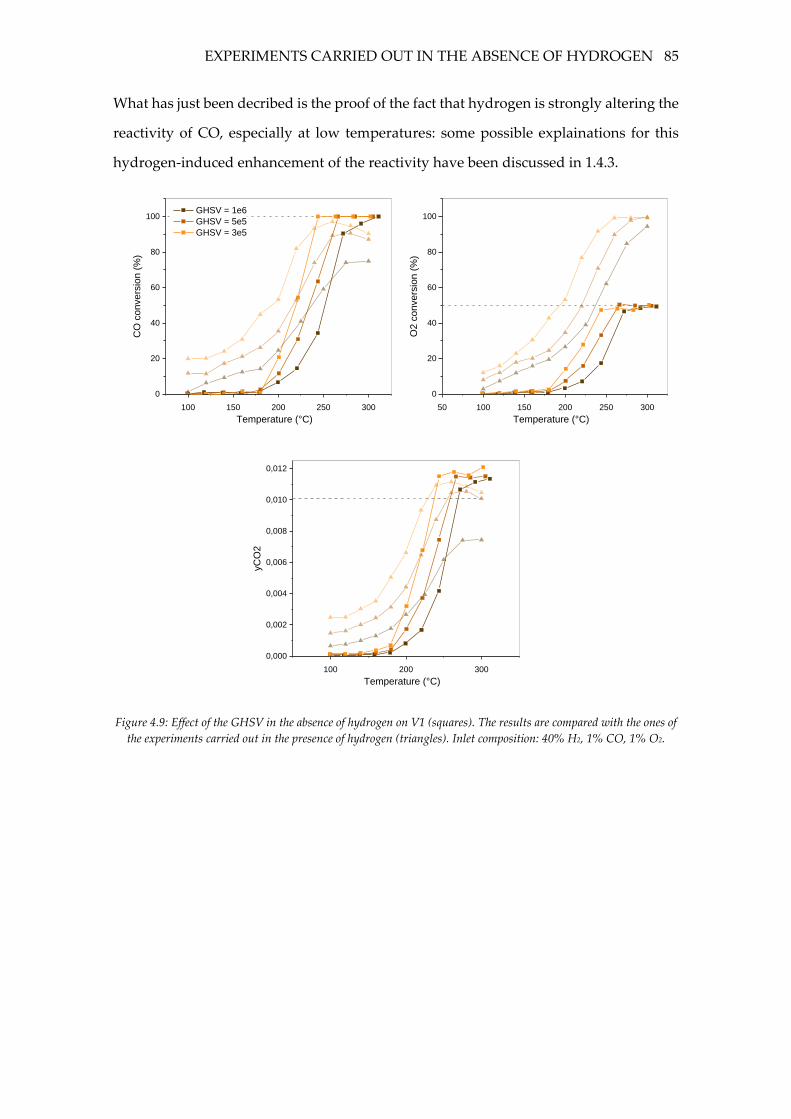
EXPERIMENTS CARRIED OUT IN THE ABSENCE OF HYDROGEN 85
What has just been decribed is the proof of the fact that hydrogen is strongly altering the
reactivity of CO, especially at low temperatures: some possible explainations for this
hydrogen-induced enhancement of the reactivity have been discussed in 1.4.3.
100 150 200 250 300
0
20
40
60
80
100 GHSV = 1e6
GHSV = 5e5
GHSV = 3e5
CO
co
nve
rsio
n (
%)
Temperature (°C)
50 100 150 200 250 300
0
20
40
60
80
100
O2 c
on
ve
rsio
n (
%)
Temperature (°C)
100 200 300
0,000
0,002
0,004
0,006
0,008
0,010
0,012
yC
O2
Temperature (°C)
Figure 4.9: Effect of the GHSV in the absence of hydrogen on V1 (squares). The results are compared with the ones of
the experiments carried out in the presence of hydrogen (triangles). Inlet composition: 40% H2, 1% CO, 1% O2.
86 EXPERIMENTS IN THE ANNULAR REACTOR
4.3.3 Effect of yO2
The effect of yO2 in the absence of hydrogen was investigated by performing tests at
0.25%, 0.5%, 0.75%, 1% and 2% concentrations. Hence, both under- and over-
stoichiometric oxygen amounts are taken into consideration. The results are reported in
Figure 4.10. For the sake of clarity, the curves obtained for the corresponding
experiments in the presence of hydrogen are not reported in the graphs.
As it can be observed, CO conversion is higher at higher oxygen concentrations. Again,
almost no conversion is observed until a certain temperature, which appears to be
slightly lower for higher oxygen concentrations. Differently from the curves obtained in
the presence of hydrogen, CO conversion monotonically increases and shows no
decreasing branch: again, no reaction other than CO oxidation can take place. In the cases
of over-stoichiometric oxygen, 100% equilibrium conversion is achieved, at a
temperature which is lower at higher oxygen concentrations.
By observing the graph for O2 conversion, almost no consumption of oxygen is seen until
200 °C, differently from the case of the hydrogen-rich system. The curves are almost
overlapped at low temperature, and then split. Oxygen conversion increases
monotonically, until reaching the equilibrium conversion (except for the 0.25% and the
0.5% tests).
Finally, CO2 concentration is clearly higher for higher oxygen amounts. This trend is an
indication of the fact that the reaction depends with a positive order on the partial
pressure of oxygen.
EXPERIMENTS CARRIED OUT IN THE ABSENCE OF HYDROGEN 87
100 150 200 250 300
0
20
40
60
80
100 O2 2%
O2 1%
O2 0.75%
O2 0.5%
O2 0.25%
CO
co
nve
rsio
n (
%)
Temperature (°C)
50 100 150 200 250 300
0
20
40
60
80
100 O2 2%
O2 1%
O2 0.75%
O2 0.5%
O2 0.25%
O2 c
on
ve
rsio
n (
%)
Temperature (°C)
100 200 300
0,000
0,002
0,004
0,006
0,008
0,010
0,012 O2 2%
O2 1%
O2 0.75%
O2 0.5%
O2 0.25%
yC
O2
Temperature (°C)
Figure 4.10: Effect of oxygen concentration on V1 in the absence of hydrogen. GHSV=500000 NL/h/kg.
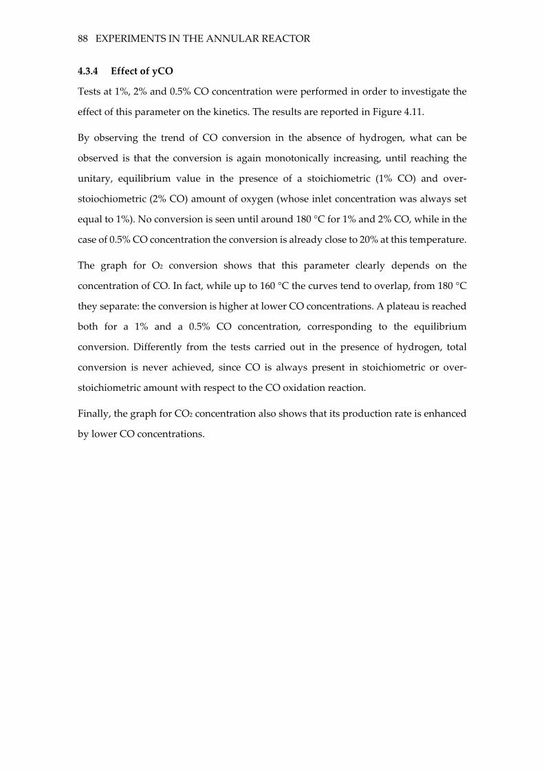
88 EXPERIMENTS IN THE ANNULAR REACTOR
4.3.4 Effect of yCO
Tests at 1%, 2% and 0.5% CO concentration were performed in order to investigate the
effect of this parameter on the kinetics. The results are reported in Figure 4.11.
By observing the trend of CO conversion in the absence of hydrogen, what can be
observed is that the conversion is again monotonically increasing, until reaching the
unitary, equilibrium value in the presence of a stoichiometric (1% CO) and over-
stoiochiometric (2% CO) amount of oxygen (whose inlet concentration was always set
equal to 1%). No conversion is seen until around 180 °C for 1% and 2% CO, while in the
case of 0.5% CO concentration the conversion is already close to 20% at this temperature.
The graph for O2 conversion shows that this parameter clearly depends on the
concentration of CO. In fact, while up to 160 °C the curves tend to overlap, from 180 °C
they separate: the conversion is higher at lower CO concentrations. A plateau is reached
both for a 1% and a 0.5% CO concentration, corresponding to the equilibrium
conversion. Differently from the tests carried out in the presence of hydrogen, total
conversion is never achieved, since CO is always present in stoichiometric or over-
stoichiometric amount with respect to the CO oxidation reaction.
Finally, the graph for CO2 concentration also shows that its production rate is enhanced
by lower CO concentrations.
EXPERIMENTS CARRIED OUT IN THE ABSENCE OF HYDROGEN 89
100 150 200 250 300
0
20
40
60
80
100 CO 2%
CO 1%
CO 0.5%
CO
co
nve
rsio
n (
%)
Temperature (°C)
50 100 150 200 250 300
0
20
40
60
80
100 CO 2%
CO 1%
CO 0.5%
O2 c
on
ve
rsio
n (
%)
Temperature (°C)
100 200 300
0,000
0,002
0,004
0,006
0,008
0,010
0,012
0,014
0,016
0,018
0,020
0,022
yC
O2
Temperature (°C)
Figure 4.11: Effect of CO concentration on V1 in the absence of hydrogen. GHSV=500000 NL/h/kg.
5 KINETIC STUDY
5.1 INTRODUCTION
5.1.1 Rate of the reaction
By considering a generic reaction:
𝜈𝐴𝐴 + 𝜈𝐵𝐵 → 𝜈𝐶𝐶 + 𝜈𝐷𝐷
The change in the number of moles of a species per unit of time is defined as the rate of
production (or disappearance) of a species. The following equalities hold:
−1
𝜈𝐴
𝑑𝑛𝐴𝑑𝑡
= −1
𝜈𝐵
𝑑𝑛𝐵𝑑𝑡
=1
𝜈𝐶
𝑑𝑛𝐶𝑑𝑡
=1
𝜈𝐷
𝑑𝑛𝐷𝑑𝑡
and each of these quantities can be considered the rate of the reaction [44], usually
expressed on an intensive basis such as the reaction volume or, in the case of
heterogeneous reactions, the mass of catalyst.
The rate of a reaction can be expressed as a function of the temperature, the pressure and
the concentrations of the species which are present in the system:
ℜ = ℜ(𝑇, 𝑃, 𝐜)
By separating the dependence on the temperature from the one on the concentrations:
ℜ(𝑇, 𝒄) = 𝑘(𝑇) ∙ 𝑓(𝒄)
𝑘(𝑇) is a proportionality factor called kinetic constant, usually expressed through
Arrhenius’ law:
𝑘(𝑇) = 𝐴𝑒𝑥𝑝 (−𝐸𝑎𝑅𝑇)
𝐴 is the so-called pre-exponential factor and 𝐸𝑎 is the activation energy. By this law, by
plotting the logarithm of the kinetic constant against 1 𝑇⁄ , a straight line of slope 𝐸𝑎
𝑅⁄ is
obtained.
A modified form of Arrenhius’ law can also be exploited:
𝑘(𝑇) = 𝐴𝑒𝑥𝑝 [−𝐸𝑎𝑅(1
𝑇−
1
𝑇𝑟𝑒𝑓)]
INTRODUCTION 91
𝑓(𝒄) can be expressed both as a function of the concentrations (usually in the case of
liquid-phase reactions) or of the partial pressures (in the case of gas-phase reactions). For
highly non-ideal systems, fugacities might replace these quantities.
The simplest way to express 𝑓(𝒄) is the following:
𝑓(𝒄) =∏𝑐𝑖𝛼𝑖
𝑁𝐶
𝑖=1
or𝑓(𝒄) =∏𝑃𝑖𝛼𝑖
𝑁𝐶
𝑖=1
where 𝛼𝑖 is the reaction order with respect to species i. The sum of the reaction orders is
defined global order of the reaction. The reaction rate will be expressed as:
ℜ(𝑇, 𝒄) = 𝑘(𝑇) ∙∏𝑐𝑖𝛼𝑖
𝑁𝐶
𝑖=1
This kind of expression is usually defined power-law. Only in the case of elementary
reactions, the reaction orders strictly coincide with the stoichiometric coefficients of the
reactants, so that:
ℜ(𝑇, 𝒄) = 𝑘(𝑇) ∙ ∏ 𝑐𝑖𝜈𝑖
𝑁𝑟𝑒𝑎𝑐𝑡𝑎𝑛𝑡𝑠
𝑖=1
If obtained through the fitting of experimental data, as it is common, the reaction orders
have however no particular physical meaning, since the overall reaction is just the result
of a series of elementary steps. Hence, the reaction orders can be positive, null, or even
negative. A limit of this approach is that a power-law expression is usually unreliable
outside of the investigated range of operating conditions.
An alternative approach is the mechanistic one. A series of elementary steps are
identified: then, by means of reasonable assumptions, the rates of the single steps are
reduced to the rate of a global reaction, which will be function of the concentrations of
stable species. The final expression is usually very accurate, but such a method requires
a deep knowledge of the reacting system. Moreover, it is quite often time-expensive and
heavy from a computational point of view.
Two main things have to be derived from a kinetic analysis: the reaction order, both
global or partial with respect to each of the species, and the kinetic constant (in terms of
pre-exponential factor, and activation energy). The kinetic analysis can be carried out
either in the differential, or in the integral regime.
92 KINETIC STUDY
5.1.2 Kinetic analysis in differential regime
If the concentration of the reactants and the temperature do not change significantly
along the reactor, the reaction rate can also be deemed constant. If this is the case, the
behaviour of the reactor is defined differential.
By considering, for instance, the oxidation of CO alone, the reaction rate can be expressed
as a function of the inlet concentrations:
ℜ = 𝑘𝑃𝐶𝑂𝛼 𝑃𝑂2
𝛽= 𝑘𝑃𝐶𝑂,𝑖𝑛
𝛼 𝑃𝑂2,𝑖𝑛𝛽
and it can be directly calculated from the experimental data starting from the molar flow
rate of the product, and the mass of catalyst in the bed:
ℜ =�̇�𝐶𝑂2𝑊𝑐𝑎𝑡
By separating the effects of CO and oxygen (the subscript in is omitted):
ℜ = 𝑘𝐶𝑂𝑃𝐶𝑂𝛼
ℜ = 𝑘𝑂2𝑃𝑂2𝛽
and linearizing:
ln(ℜ) = ln(𝑘𝐶𝑂) + 𝛼ln(𝑃𝐶𝑂)
ln(ℜ) = ln(𝑘𝑂2) + 𝛽ln(𝑃𝑂2)
By means of a simple linear interpolation, the reaction orders 𝛼 and 𝛽 can be estimated.
It must be underlined that the differential approach can be exploited only as long as the
conversion of the limiting reactant is below a certain threshold, which depends on the
sensitivity of the system. For this analysis, it has been assumed equal to 20%.
Above this threshold, the variation in the reaction rate along the reactor cannot be
deemed negligible anymore, and an integral analysis should be carried out instead.
MATHEMATICAL MODEL OF THE ANNULAR REACTOR 93
5.2 MATHEMATICAL MODEL OF THE ANNULAR REACTOR
5.2.1 Introduction
The kinetic parameters were derived through the comparison of the experimental data
with the results obtained from a model for an isothermal plug-flow reactor. Such model
was developed [45] for the simulation of the catalytic partial oxidation of methane on a
Rh/Al2O3 catalyst inside an annular reactor: hence, the kinetic scheme had to be
extensively modified.
The main features of the model are the following:
• one-dimensional PFR, heterogeneous (all the radial gradient are localized inside
an infinitesimal layer by the catalytic suface);
• negligible axial dispersion (high value of the axial Péclet number);
• laminar flow;
• isothermal (temperature gradients are absent both in the axial direction and
between the bed and the gas phase).
The reactor can be considered isothermal as long as the temperature difference along the
bed does not exceed 10 °C. If such assumption is not valid, the temperature profile is
estimated by means of a fifth-order polynomial in the axial coordinate, as follows:
𝑇(𝑧) = 𝑎1𝑧5 + 𝑎2𝑧
4 + 𝑎3𝑧3 + 𝑎4𝑧
2 + 𝑎5𝑧 + 𝑎6
Both interphase and intraphase mass transfer limitations can be accounted for.
5.2.2 Equations of the model
Since the model is heterogeneous, it can be used to estimate the concentration profiles
along the axis for both the gas phase and the surface of the solid. The number of
unknowns of the problem is 2NC, i.e. NC surface concentrations 𝑥𝑖𝑆 and NC
concentrations 𝑥𝑖𝐵 in the bulk of the gas phase, where NC is the number of components.
To solve the problem, 2NC equations have to be written. In particular:
• NC mass balance equations for the gas phase, in adimensional terms:
𝑃𝑒𝑚,𝑖𝑑𝐹𝑖
∗
𝑑𝑧∗= −
4
1 +1𝑅∗
𝑆ℎ𝑙𝑜𝑐,𝑖(𝑥𝑖𝐵 − 𝑥𝑖
𝑆)𝐹𝑡𝑜𝑡
𝐹𝑡𝑜𝑡0
where 𝑆ℎ𝑙𝑜𝑐,𝑖 is the local Sherwood number (see next paragraph), and:
94 KINETIC STUDY
𝑃𝑒𝑚,𝑖 =�̅�𝐷ℎ𝑦𝑑𝑟
𝒟𝑖
𝐷ℎ𝑦𝑑𝑟 = 𝐷𝑜𝑢𝑡 − 𝐷𝑖𝑛
𝑧∗ =𝑧
𝐷ℎ𝑦𝑑𝑟
𝐹𝑖∗ =
𝐹𝑖
𝐹𝑡𝑜𝑡0
𝑅∗ =𝐷𝑖𝑛𝐷𝑜𝑢𝑡
Of the NC ordinary differential equations, three can be replaced by the atomic
balances for the bulk phase on carbon, hydrogen and oxygen. In fact, being the
atomic balances first-order linear, algebraic equations, the replacement leads to
a significant simplification of the model and thus to a reduction of the
computational time.
∑(𝐹𝑖 − 𝐹𝑖0)𝑛𝐶,𝑖 = 0
𝑁𝐶
𝑖=1
∑(𝐹𝑖 − 𝐹𝑖0)𝑛𝐻,𝑖 = 0
𝑁𝐶
𝑖=1
∑(𝐹𝑖 − 𝐹𝑖0)𝑛𝑂,𝑖 = 0
𝑁𝐶
𝑖=1
• NC continuity equations for the catalyst phase:
𝑆ℎ𝑙𝑜𝑐,𝑖(𝑥𝑖𝐵 − 𝑥𝑖
𝑆) =∑𝜈𝑖,𝑗𝛼𝑖ℜ𝑗
𝑁𝑅
𝑗=1
where ℜ𝑗 is the reaction rate of the j-th reaction, and:
𝛼𝑖 =𝐷ℎ𝑦𝑑𝑟𝑊𝑐𝑎𝑡
𝑆𝒟𝑖𝑐𝑡𝑜𝑡
𝑊𝑐𝑎𝑡 is the mass of catalyst and 𝑆 its surface area. 𝑐𝑡𝑜𝑡 is the total concentration in
the gas phase, calculated under the assumption of mixture of ideal gases as 𝑃/𝑅𝑇.
𝒟𝑖 is the molecular diffusivity of species i and is approximated as the binary
diffusivity of species i in nitrogen, calculated according to the Fuller-Schletter-
Giddings correlation.
The 2NC equations can be solved by means of numerical methods.
MATHEMATICAL MODEL OF THE ANNULAR REACTOR 95
5.2.3 Mass transfer resistances
To account for the presence of interphase mass transfer resistances, the following
expression is used for the estimation of the axial profile of the local Sherwood number:
𝑆ℎ𝑙𝑜𝑐,𝑖(𝑧𝑆ℎ,𝑖) = 𝑆ℎ𝑖𝑛𝑓 + 6.874exp(−71.2𝑧𝑆ℎ,𝑖)(1000𝑧𝑆ℎ,𝑖)−0.35
where
𝑧𝑆ℎ,𝑖 =𝑧∗
𝑃𝑒𝑚,𝑖
𝑆ℎ𝑖𝑛𝑓 = 6.6156 − 1.7548𝑅∗
The functional form of the expression for 𝑆ℎ𝑙𝑜𝑐,𝑖(𝑧𝑆ℎ,𝑖) had already been used in the
literature for the interpolation of the exact solutions of the Graetz-Nusselt problem (and
analogous mass transfer problems) in ducts of various geometries. The coefficients have
been derived by adapting the expression to an annular geometry with boundary
conditions of the third-type [43].
The model is also capable of accounting for intraphase mass transfer limitations by
means of a generalized efficiency factor for oxygen (and also for methane in the original
model [45]). Indeed, the oxidation rates are assumed to be limited by oxygen: this effect
is included by multiplying each of the two rates by the efficiency factor.
At least as a first approximation, internal mass transfer resistances were not considered
in the modelling phase. Thus, the derived kinetic expressions already account for the
presence of diffusion limitations inside the washcoat: being its thickness close to the one
of the active phase of the catalytic pellet, the expression for the reaction rate should still
be valid. However, the impact of internal mass transfer limitations on the results is still
to be verified in a second moment.
5.2.4 Reaction rates
The overall rate of production (or consumption) of species i is calculated as:
𝑟𝑖 =∑𝜈𝑖,𝑗ℜ𝑗
𝑁𝑅
𝑗=1
where ℜ𝑗 is the rate of the j-th reaction. The kinetic scheme [45] used in the model was
developed for methane CPO on Rh and includes seven reactions: total oxidation of
methane; steam reforming of methane; water gas shift and reverse water gas shift;
96 KINETIC STUDY
methanation; H2 oxidation; CO oxidation. Since none of the original expressions for the
reaction rates has been used in this work, the seven-reaction kinetic scheme will not be
reported here for the sake of brevity. It is only worth underlining that WGS and rWGS
are expressed through two distinct expressions, since it was proven that it is not possible
to use one single equation to describe both the direct and the reverse steps.
In the case of CO oxidation in the absence of hydrogen, one single reaction is to be
considered: CO oxidation. In the case of CO PrOx, four of the original seven reactions
are in principle to be taken into account: the two oxidations, the water gas shift reaction
and the reverse water gas shift.
All the reaction rates had to be derived basically from scratch: the details of the
derivation are reported in the following paragraphs.
5.3 STUDY OF CO OXIDATION IN THE ABSENCE OF HYDROGEN
5.3.1 Introduction
Before performing a kinetic study on the oxidation of carbon monoxide in a hydrogen-
rich environment, an attempt was made to derive a kinetic expression for the oxidation
of CO alone. The effect of the concentration of CO and oxygen on the kinetics was
investigated through a number of tests performed at a GHSV=500000 NL/h/kg, in the
100-300 °C temperature range. The experiments have been discussed in depth in 4.3.
First, a differential analysis was performed by using low-conversion data to obtain a
power-law like expression for the reaction rate:
ℜ = 𝑘𝑃𝐶𝑂𝛼 𝑃𝑂2
𝛽
Then, starting from the results of the differential analysis, a more elaborate expression
was developed by exploiting the mathematical model of the annular reactor: the kinetic
parameters were properly modified by comparing the results of the model to the
experimental data.
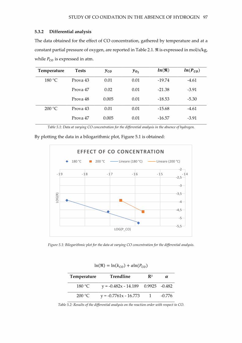
STUDY OF CO OXIDATION IN THE ABSENCE OF HYDROGEN 97
5.3.2 Differential analysis
The data obtained for the effect of CO concentration, gathered by temperature and at a
constant partial pressure of oxygen, are reported in Table 2.1. ℜ is expressed in mol/s/kg,
while 𝑃𝐶𝑂 is expressed in atm.
Temperature Tests 𝒚𝑪𝑶 𝒚𝑶𝟐 𝒍𝒏(𝕽) 𝒍𝒏(𝑷𝑪𝑶)
180 °C Prova 43
Prova 47
Prova 48
0.01
0.02
0.005
0.01
0.01
0.01
-19.74
-21.38
-18.53
-4.61
-3.91
-5.30
200 °C Prova 43
Prova 47
0.01
0.005
0.01
0.01
-15.68
-16.57
-4.61
-3.91
Table 5.1: Data at varying CO concentration for the differential analysis in the absence of hydrogen.
By plotting the data in a bilogarithmic plot, Figure 5.1 is obtained:
Figure 5.1: Bilogarithmic plot for the data at varying CO concentration for the differential analysis.
ln(ℜ) = ln(𝑘𝐶𝑂) + 𝛼ln(𝑃𝐶𝑂)
Temperature Trendline R2 𝜶
180 °C y = -0.482x - 14.189 0.9925 -0.482
200 °C y = -0.7761x - 16.773 1 -0.776
Table 5.2: Results of the differential analysis on the reaction order with respect to CO.
-5,5
-5
-4,5
-4
-3,5
-3
-2,5
-2
- 1 9 - 1 8 - 1 7 - 1 6 - 1 5 - 1 4
LOG
(R)
LOG(P_CO)
EFFECT OF CO CONCENTRATION
180 °C 200 °C Lineare (180 °C) Lineare (200 °C)
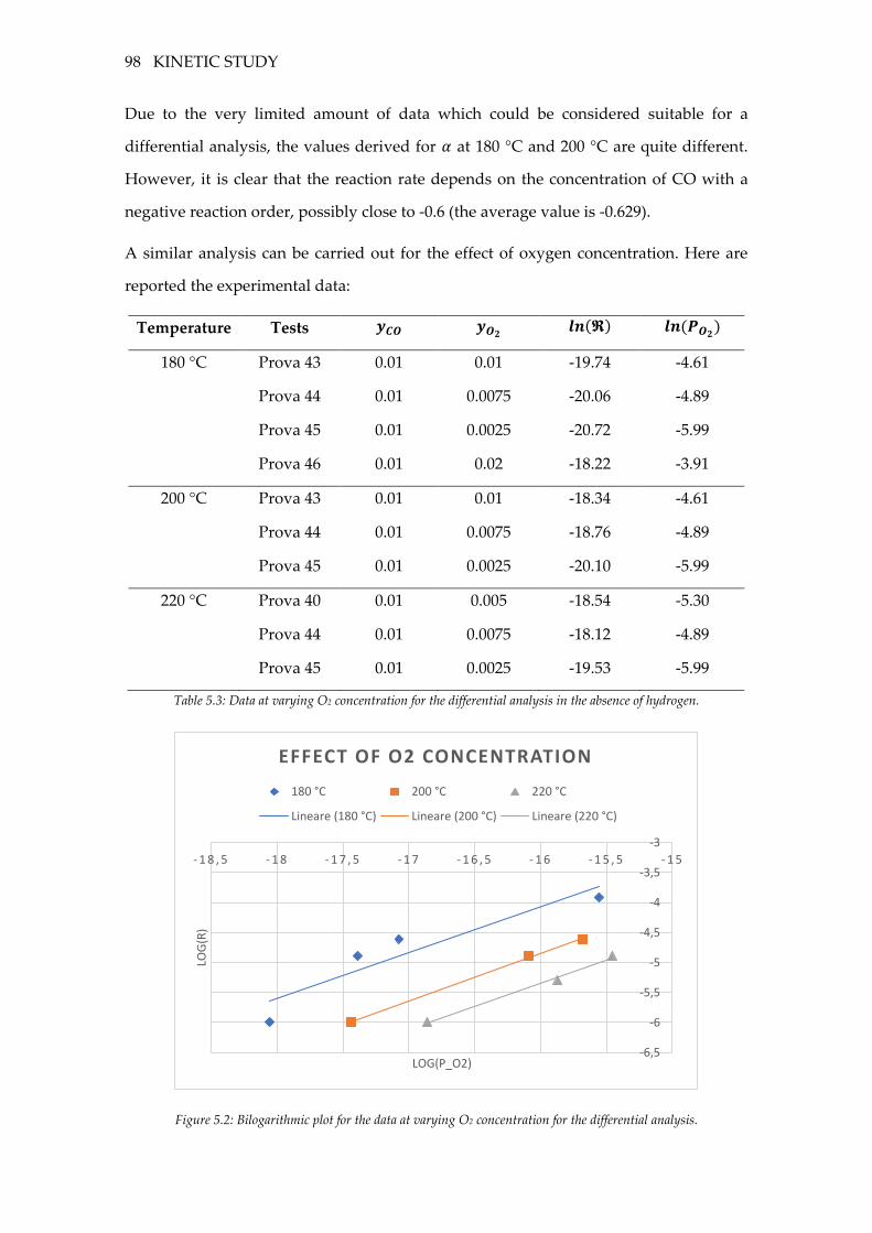
98 KINETIC STUDY
Due to the very limited amount of data which could be considered suitable for a
differential analysis, the values derived for 𝛼 at 180 °C and 200 °C are quite different.
However, it is clear that the reaction rate depends on the concentration of CO with a
negative reaction order, possibly close to -0.6 (the average value is -0.629).
A similar analysis can be carried out for the effect of oxygen concentration. Here are
reported the experimental data:
Temperature Tests 𝒚𝑪𝑶 𝒚𝑶𝟐 𝒍𝒏(𝕽) 𝒍𝒏(𝑷𝑶𝟐)
180 °C Prova 43
Prova 44
Prova 45
Prova 46
0.01
0.01
0.01
0.01
0.01
0.0075
0.0025
0.02
-19.74
-20.06
-20.72
-18.22
-4.61
-4.89
-5.99
-3.91
200 °C Prova 43
Prova 44
Prova 45
0.01
0.01
0.01
0.01
0.0075
0.0025
-18.34
-18.76
-20.10
-4.61
-4.89
-5.99
220 °C Prova 40
Prova 44
Prova 45
0.01
0.01
0.01
0.005
0.0075
0.0025
-18.54
-18.12
-19.53
-5.30
-4.89
-5.99
Table 5.3: Data at varying O2 concentration for the differential analysis in the absence of hydrogen.
Figure 5.2: Bilogarithmic plot for the data at varying O2 concentration for the differential analysis.
-6,5
-6
-5,5
-5
-4,5
-4
-3,5
-3
- 1 8 , 5 - 1 8 - 1 7 , 5 - 1 7 - 1 6 , 5 - 1 6 - 1 5 , 5 - 1 5
LOG
(R)
LOG(P_O2)
EFFECT OF O2 CONCENTRATION
180 °C 200 °C 220 °C
Lineare (180 °C) Lineare (200 °C) Lineare (220 °C)
STUDY OF CO OXIDATION IN THE ABSENCE OF HYDROGEN 99
The results are the following:
ln(ℜ) = ln(𝑘𝑂2) + 𝛽ln(𝑃𝑂2)
Temperature Trendline R2 𝜷
180 °C y = 0.7635x + 10.18 0.869 0.764
200 °C y = 0.7951x + 9.9981 0.9991 0.795
220 °C y = 0.7683x + 8.9943 0.9929 0.768
Table 5.4: Results of the differential analysis on the reaction order with respect to O2.
In this case, the results are in very good agreement with each other. The reaction order
with respect to oxygen is positive, and its value is close to 0.8 (the average value is 0.776).
Thus, the analysis of single orders suggests a power-law expression for the oxidation of
CO in the absence of hydrogen as the following:
ℜ = 𝑘𝑃𝐶𝑂−0.63𝑃𝑂2
0.78
The result is in line with the literature.
5.3.3 Integration of CO oxidation into the model of the annular reactor
First of all, all the reactions but CO oxidation were removed from the original model of
the annular reactor, by zeroing their kinetic constant. Then, the kinetics of CO oxidation
was properly modified.
A power-law expression like the one obtained through the differential analysis would
have been inadequate for the simulation of the whole conversion range. In fact, since the
reaction rate is expressed as:
ℜ = 𝑘𝑃𝑂2𝛽
𝑃𝐶𝑂𝛼
as the conversion of CO tends to 1, the reaction rate tends to infinite, leading to numerical
issues. Thus, instead of using a simple expression like the one above, an expression based
on a reaction path was developed.
It is clear from the experimental results that, at least on a Pt-type catalyst, the reaction is
inhibited by CO and enhanced by oxygen: thus, a negative reaction order can be
expected for the first species, and a positive one for the second. This is confirmed in the
literature for the so-called low-rate branch. CO oxidation is indeed characterized by two
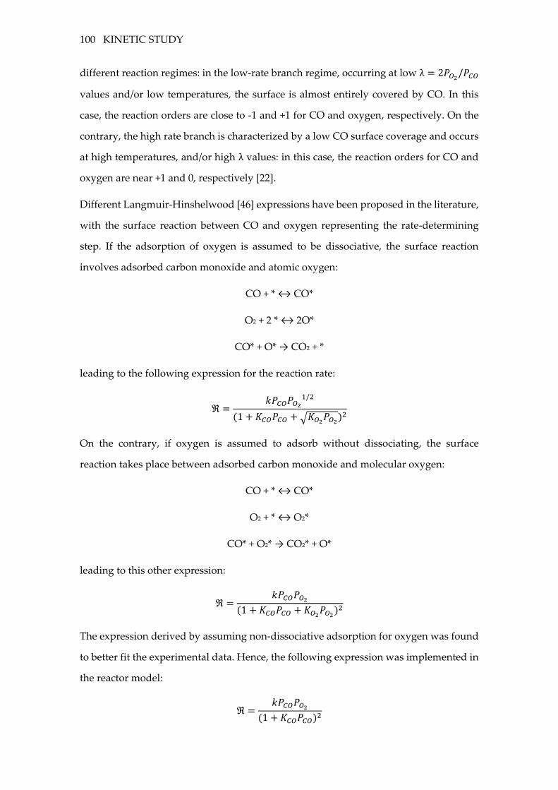
100 KINETIC STUDY
different reaction regimes: in the low-rate branch regime, occurring at low λ = 2𝑃𝑂2/𝑃𝐶𝑂
values and/or low temperatures, the surface is almost entirely covered by CO. In this
case, the reaction orders are close to -1 and +1 for CO and oxygen, respectively. On the
contrary, the high rate branch is characterized by a low CO surface coverage and occurs
at high temperatures, and/or high λ values: in this case, the reaction orders for CO and
oxygen are near +1 and 0, respectively [22].
Different Langmuir-Hinshelwood [46] expressions have been proposed in the literature,
with the surface reaction between CO and oxygen representing the rate-determining
step. If the adsorption of oxygen is assumed to be dissociative, the surface reaction
involves adsorbed carbon monoxide and atomic oxygen:
CO + * ↔ CO*
O2 + 2 * ↔ 2O*
CO* + O* → CO2 + *
leading to the following expression for the reaction rate:
ℜ =𝑘𝑃𝐶𝑂𝑃𝑂2
1/2
(1 + 𝐾𝐶𝑂𝑃𝐶𝑂 + √𝐾𝑂2𝑃𝑂2)2
On the contrary, if oxygen is assumed to adsorb without dissociating, the surface
reaction takes place between adsorbed carbon monoxide and molecular oxygen:
CO + * ↔ CO*
O2 + * ↔ O2*
CO* + O2* → CO2* + O*
leading to this other expression:
ℜ =𝑘𝑃𝐶𝑂𝑃𝑂2
(1 + 𝐾𝐶𝑂𝑃𝐶𝑂 + 𝐾𝑂2𝑃𝑂2)2
The expression derived by assuming non-dissociative adsorption for oxygen was found
to better fit the experimental data. Hence, the following expression was implemented in
the reactor model:
ℜ =𝑘𝑃𝐶𝑂𝑃𝑂2
(1 + 𝐾𝐶𝑂𝑃𝐶𝑂)2
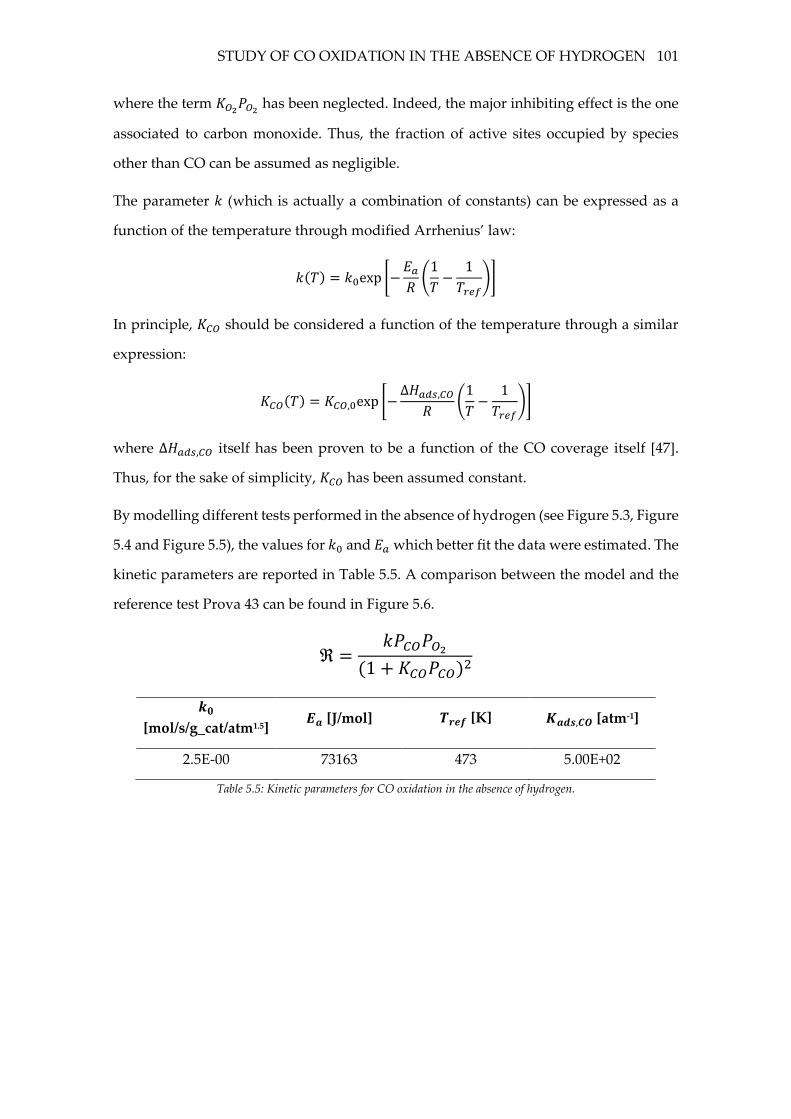
STUDY OF CO OXIDATION IN THE ABSENCE OF HYDROGEN 101
where the term 𝐾𝑂2𝑃𝑂2 has been neglected. Indeed, the major inhibiting effect is the one
associated to carbon monoxide. Thus, the fraction of active sites occupied by species
other than CO can be assumed as negligible.
The parameter 𝑘 (which is actually a combination of constants) can be expressed as a
function of the temperature through modified Arrhenius’ law:
𝑘(𝑇) = 𝑘0exp [−𝐸𝑎𝑅(1
𝑇−
1
𝑇𝑟𝑒𝑓)]
In principle, 𝐾𝐶𝑂 should be considered a function of the temperature through a similar
expression:
𝐾𝐶𝑂(𝑇) = 𝐾𝐶𝑂,0exp [−∆𝐻𝑎𝑑𝑠,𝐶𝑂
𝑅(1
𝑇−
1
𝑇𝑟𝑒𝑓)]
where ∆𝐻𝑎𝑑𝑠,𝐶𝑂 itself has been proven to be a function of the CO coverage itself [47].
Thus, for the sake of simplicity, 𝐾𝐶𝑂 has been assumed constant.
By modelling different tests performed in the absence of hydrogen (see Figure 5.3, Figure
5.4 and Figure 5.5), the values for 𝑘0 and 𝐸𝑎 which better fit the data were estimated. The
kinetic parameters are reported in Table 5.5. A comparison between the model and the
reference test Prova 43 can be found in Figure 5.6.
ℜ =𝑘𝑃𝐶𝑂𝑃𝑂2
(1 + 𝐾𝐶𝑂𝑃𝐶𝑂)2
𝒌𝟎
[mol/s/g_cat/atm1.5] 𝑬𝒂 [J/mol] 𝑻𝒓𝒆𝒇 [K] 𝑲𝒂𝒅𝒔,𝑪𝑶 [atm-1]
2.5E-00 73163 473 5.00E+02
Table 5.5: Kinetic parameters for CO oxidation in the absence of hydrogen.
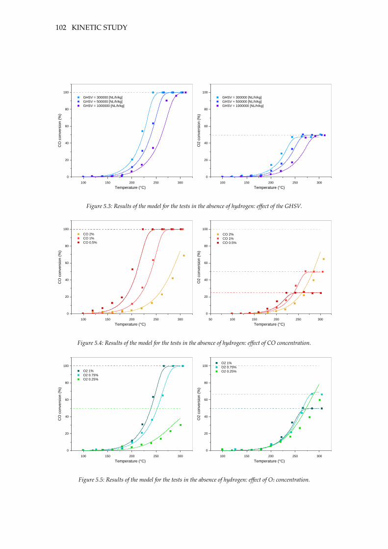
102 KINETIC STUDY
100 150 200 250 300
0
20
40
60
80
100
GHSV = 300000 [NL/h/kg]
GHSV = 500000 [NL/h/kg]
GHSV = 1000000 [NL/h/kg]
CO
co
nve
rsio
n (
%)
Temperature (°C)
100 150 200 250 300
0
20
40
60
80
100
GHSV = 300000 [NL/h/kg]
GHSV = 500000 [NL/h/kg]
GHSV = 1000000 [NL/h/kg]
O2
co
nve
rsio
n (
%)
Temperature (°C)
Figure 5.3: Results of the model for the tests in the absence of hydrogen: effect of the GHSV.
100 150 200 250 300
0
20
40
60
80
100
CO 2%
CO 1%
CO 0.5%
CO
co
nvers
ion
(%
)
Temperature (°C)
50 100 150 200 250 300
0
20
40
60
80
100
CO 2%
CO 1%
CO 0.5%
O2 c
on
ve
rsio
n (
%)
Temperature (°C)
Figure 5.4: Results of the model for the tests in the absence of hydrogen: effect of CO concentration.
100 150 200 250 300
0
20
40
60
80
100
O2 1%
O2 0.75%
O2 0.25%
CO
co
nve
rsio
n (
%)
Temperature (°C)
100 150 200 250 300
0
20
40
60
80
100 O2 1%
O2 0.75%
O2 0.25%
O2
co
nve
rsio
n (
%)
Temperature (°C)
Figure 5.5: Results of the model for the tests in the absence of hydrogen: effect of O2 concentration.
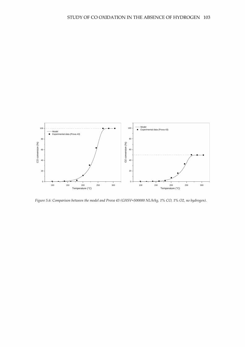
STUDY OF CO OXIDATION IN THE ABSENCE OF HYDROGEN 103
100 150 200 250 300
0
20
40
60
80
100
Model
Experimental data (Prova 43)
CO
co
nve
rsio
n (
%)
Temperature (°C)
100 150 200 250 300
0
20
40
60
80
100 Model
Experimental data (Prova 43)
O2 c
onvers
ion (
%)
Temperature (°C)
Figure 5.6: Comparison between the model and Prova 43 (GHSV=500000 NL/h/kg, 1% CO, 1% O2, no hydrogen).
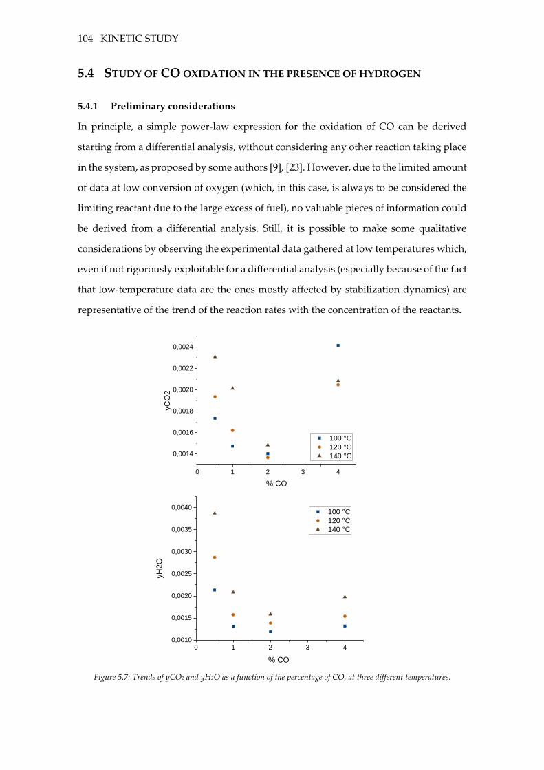
104 KINETIC STUDY
5.4 STUDY OF CO OXIDATION IN THE PRESENCE OF HYDROGEN
5.4.1 Preliminary considerations
In principle, a simple power-law expression for the oxidation of CO can be derived
starting from a differential analysis, without considering any other reaction taking place
in the system, as proposed by some authors [9], [23]. However, due to the limited amount
of data at low conversion of oxygen (which, in this case, is always to be considered the
limiting reactant due to the large excess of fuel), no valuable pieces of information could
be derived from a differential analysis. Still, it is possible to make some qualitative
considerations by observing the experimental data gathered at low temperatures which,
even if not rigorously exploitable for a differential analysis (especially because of the fact
that low-temperature data are the ones mostly affected by stabilization dynamics) are
representative of the trend of the reaction rates with the concentration of the reactants.
0 1 2 3 4
0,0014
0,0016
0,0018
0,0020
0,0022
0,0024
100 °C
120 °C
140 °C
yC
O2
% CO
0 1 2 3 40,0010
0,0015
0,0020
0,0025
0,0030
0,0035
0,0040 100 °C
120 °C
140 °C
yH
2O
% CO
Figure 5.7: Trends of yCO2 and yH2O as a function of the percentage of CO, at three different temperatures.
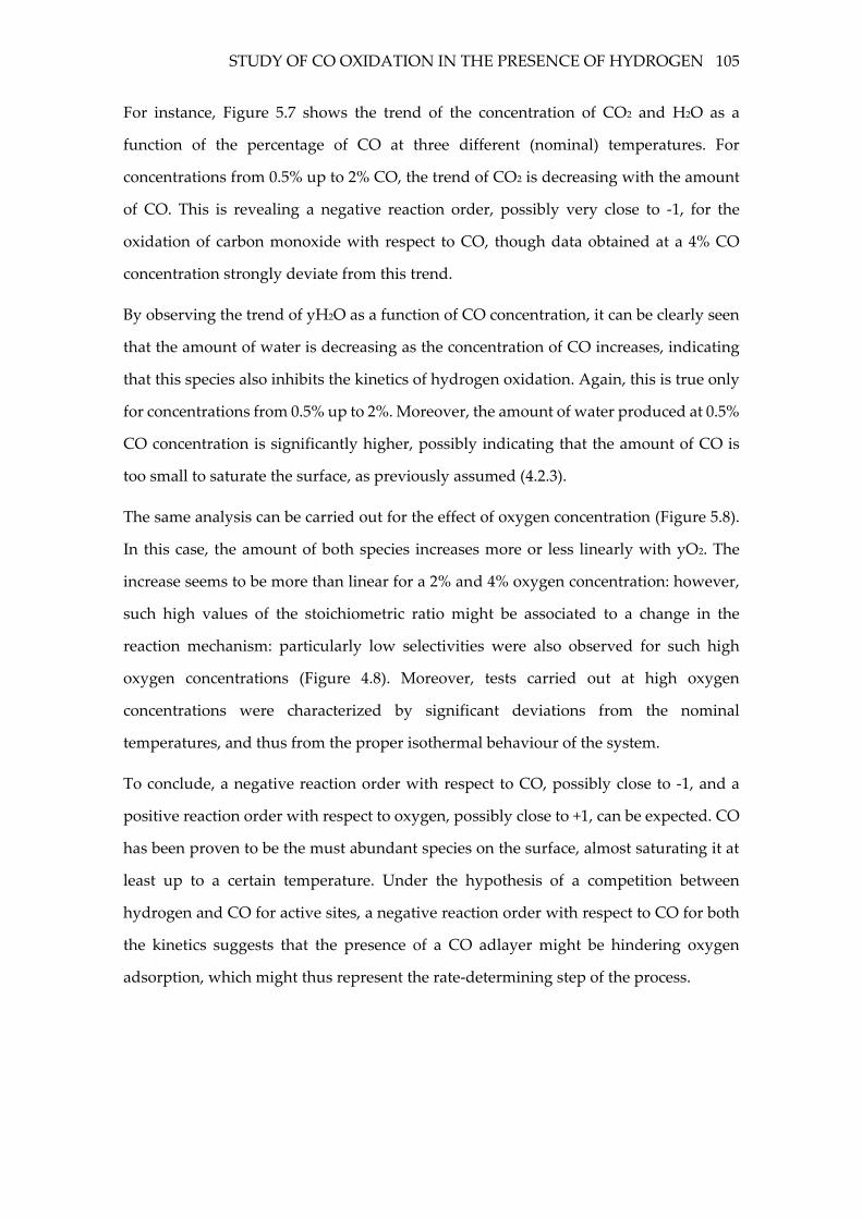
STUDY OF CO OXIDATION IN THE PRESENCE OF HYDROGEN 105
For instance, Figure 5.7 shows the trend of the concentration of CO2 and H2O as a
function of the percentage of CO at three different (nominal) temperatures. For
concentrations from 0.5% up to 2% CO, the trend of CO2 is decreasing with the amount
of CO. This is revealing a negative reaction order, possibly very close to -1, for the
oxidation of carbon monoxide with respect to CO, though data obtained at a 4% CO
concentration strongly deviate from this trend.
By observing the trend of yH2O as a function of CO concentration, it can be clearly seen
that the amount of water is decreasing as the concentration of CO increases, indicating
that this species also inhibits the kinetics of hydrogen oxidation. Again, this is true only
for concentrations from 0.5% up to 2%. Moreover, the amount of water produced at 0.5%
CO concentration is significantly higher, possibly indicating that the amount of CO is
too small to saturate the surface, as previously assumed (4.2.3).
The same analysis can be carried out for the effect of oxygen concentration (Figure 5.8).
In this case, the amount of both species increases more or less linearly with yO2. The
increase seems to be more than linear for a 2% and 4% oxygen concentration: however,
such high values of the stoichiometric ratio might be associated to a change in the
reaction mechanism: particularly low selectivities were also observed for such high
oxygen concentrations (Figure 4.8). Moreover, tests carried out at high oxygen
concentrations were characterized by significant deviations from the nominal
temperatures, and thus from the proper isothermal behaviour of the system.
To conclude, a negative reaction order with respect to CO, possibly close to -1, and a
positive reaction order with respect to oxygen, possibly close to +1, can be expected. CO
has been proven to be the must abundant species on the surface, almost saturating it at
least up to a certain temperature. Under the hypothesis of a competition between
hydrogen and CO for active sites, a negative reaction order with respect to CO for both
the kinetics suggests that the presence of a CO adlayer might be hindering oxygen
adsorption, which might thus represent the rate-determining step of the process.
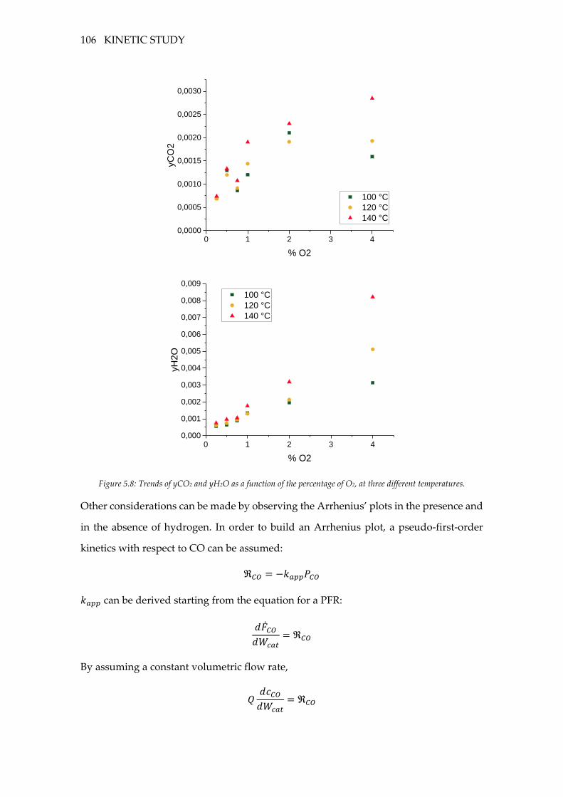
106 KINETIC STUDY
0 1 2 3 40,0000
0,0005
0,0010
0,0015
0,0020
0,0025
0,0030
100 °C
120 °C
140 °C
yC
O2
% O2
0 1 2 3 40,000
0,001
0,002
0,003
0,004
0,005
0,006
0,007
0,008
0,009
100 °C
120 °C
140 °C
yH
2O
% O2
Figure 5.8: Trends of yCO2 and yH2O as a function of the percentage of O2, at three different temperatures.
Other considerations can be made by observing the Arrhenius’ plots in the presence and
in the absence of hydrogen. In order to build an Arrhenius plot, a pseudo-first-order
kinetics with respect to CO can be assumed:
ℜ𝐶𝑂 = −𝑘𝑎𝑝𝑝𝑃𝐶𝑂
𝑘𝑎𝑝𝑝 can be derived starting from the equation for a PFR:
𝑑�̇�𝐶𝑂𝑑𝑊𝑐𝑎𝑡
= ℜ𝐶𝑂
By assuming a constant volumetric flow rate,
𝑄𝑑𝑐𝐶𝑂𝑑𝑊𝑐𝑎𝑡
= ℜ𝐶𝑂
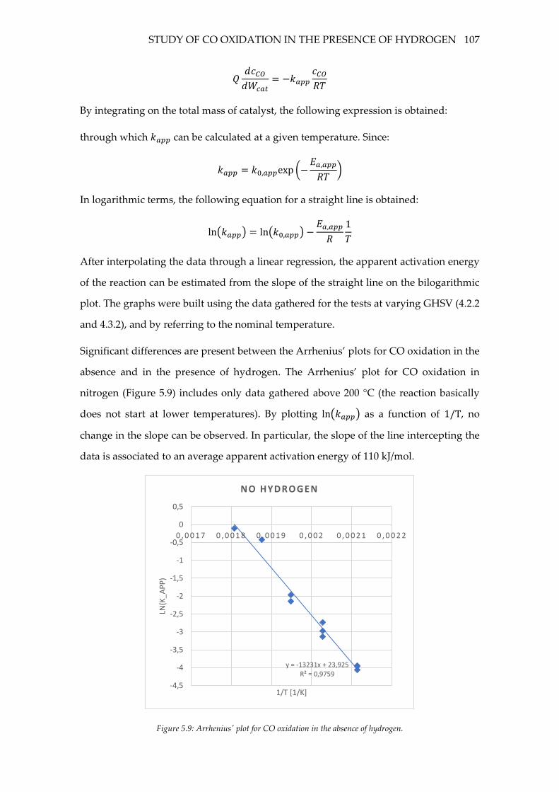
STUDY OF CO OXIDATION IN THE PRESENCE OF HYDROGEN 107
𝑄𝑑𝑐𝐶𝑂𝑑𝑊𝑐𝑎𝑡
= −𝑘𝑎𝑝𝑝𝑐𝐶𝑂𝑅𝑇
By integrating on the total mass of catalyst, the following expression is obtained:
through which 𝑘𝑎𝑝𝑝 can be calculated at a given temperature. Since:
𝑘𝑎𝑝𝑝 = 𝑘0,𝑎𝑝𝑝exp(−𝐸𝑎,𝑎𝑝𝑝
𝑅𝑇)
In logarithmic terms, the following equation for a straight line is obtained:
ln(𝑘𝑎𝑝𝑝) = ln(𝑘0,𝑎𝑝𝑝) −𝐸𝑎,𝑎𝑝𝑝
𝑅
1
𝑇
After interpolating the data through a linear regression, the apparent activation energy
of the reaction can be estimated from the slope of the straight line on the bilogarithmic
plot. The graphs were built using the data gathered for the tests at varying GHSV (4.2.2
and 4.3.2), and by referring to the nominal temperature.
Significant differences are present between the Arrhenius’ plots for CO oxidation in the
absence and in the presence of hydrogen. The Arrhenius’ plot for CO oxidation in
nitrogen (Figure 5.9) includes only data gathered above 200 °C (the reaction basically
does not start at lower temperatures). By plotting ln(𝑘𝑎𝑝𝑝) as a function of 1/T, no
change in the slope can be observed. In particular, the slope of the line intercepting the
data is associated to an average apparent activation energy of 110 kJ/mol.
Figure 5.9: Arrhenius' plot for CO oxidation in the absence of hydrogen.
y = -13231x + 23,925R² = 0,9759
-4,5
-4
-3,5
-3
-2,5
-2
-1,5
-1
-0,5
0
0,5
0 , 0 0 1 7 0 , 0 0 1 8 0 , 0 0 1 9 0 , 0 0 2 0 , 0 0 2 1 0 , 0 0 2 2
LN(K
_AP
P)
1/T [1/K]
NO HYDROGEN
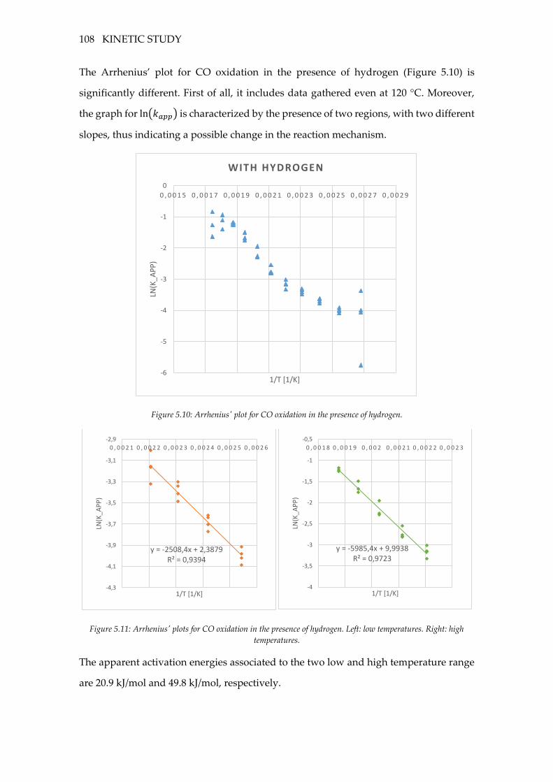
108 KINETIC STUDY
The Arrhenius’ plot for CO oxidation in the presence of hydrogen (Figure 5.10) is
significantly different. First of all, it includes data gathered even at 120 °C. Moreover,
the graph for ln(𝑘𝑎𝑝𝑝) is characterized by the presence of two regions, with two different
slopes, thus indicating a possible change in the reaction mechanism.
Figure 5.10: Arrhenius' plot for CO oxidation in the presence of hydrogen.
Figure 5.11: Arrhenius' plots for CO oxidation in the presence of hydrogen. Left: low temperatures. Right: high
temperatures.
The apparent activation energies associated to the two low and high temperature range
are 20.9 kJ/mol and 49.8 kJ/mol, respectively.
-6
-5
-4
-3
-2
-1
0
0 , 0 0 1 5 0 , 0 0 1 7 0 , 0 0 1 9 0 , 0 0 2 1 0 , 0 0 2 3 0 , 0 0 2 5 0 , 0 0 2 7 0 , 0 0 2 9
LN(K
_AP
P)
1/T [1/K]
WITH HYDROGEN
y = -2508,4x + 2,3879R² = 0,9394
-4,3
-4,1
-3,9
-3,7
-3,5
-3,3
-3,1
-2,9
0 , 0 0 2 1 0 , 0 0 2 2 0 , 0 0 2 3 0 , 0 0 2 4 0 , 0 0 2 5 0 , 0 0 2 6
LN(K
_AP
P)
1/T [1/K]
y = -5985,4x + 9,9938R² = 0,9723
-4
-3,5
-3
-2,5
-2
-1,5
-1
-0,5
0 , 0 0 1 8 0 , 0 0 1 9 0 , 0 0 2 0 , 0 0 2 1 0 , 0 0 2 2 0 , 0 0 2 3
LN(K
_AP
P)
1/T [1/K]
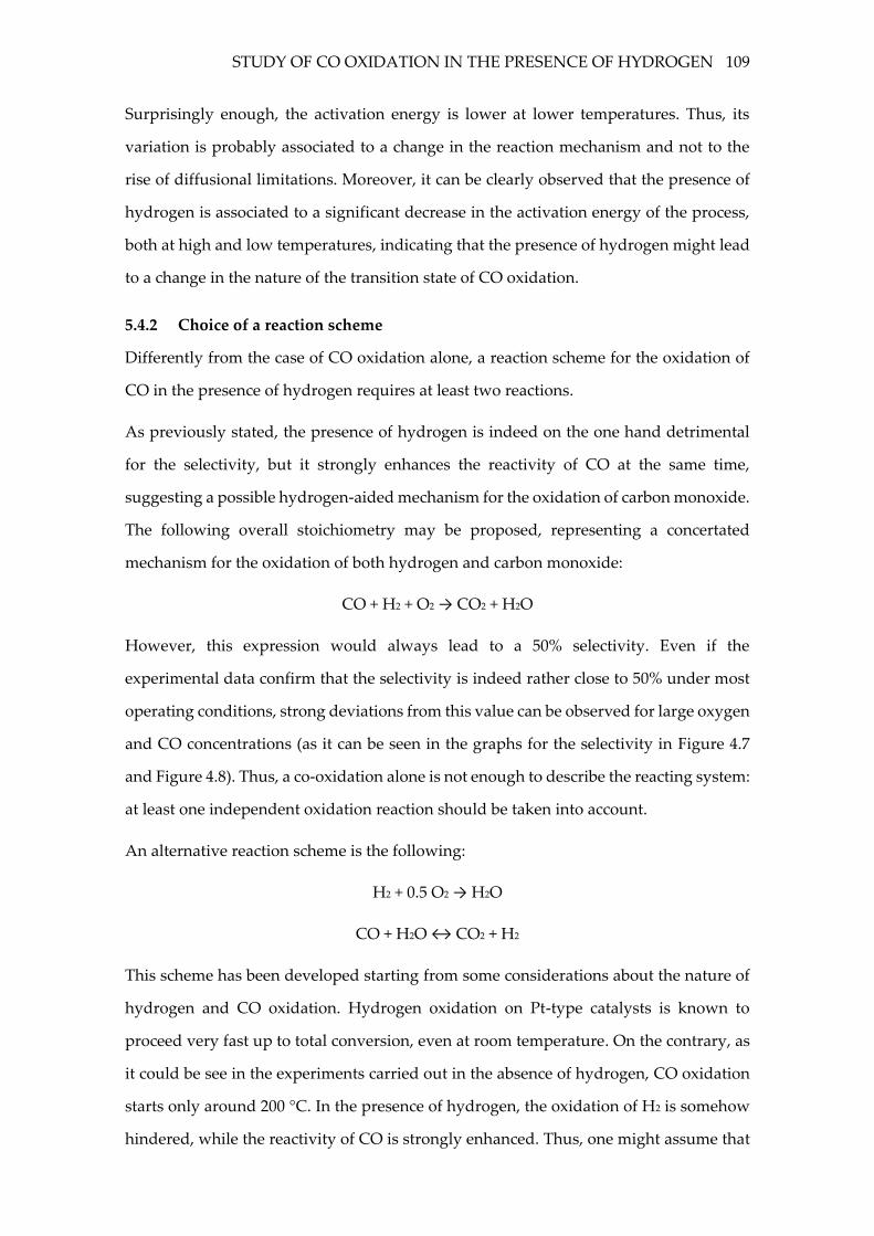
STUDY OF CO OXIDATION IN THE PRESENCE OF HYDROGEN 109
Surprisingly enough, the activation energy is lower at lower temperatures. Thus, its
variation is probably associated to a change in the reaction mechanism and not to the
rise of diffusional limitations. Moreover, it can be clearly observed that the presence of
hydrogen is associated to a significant decrease in the activation energy of the process,
both at high and low temperatures, indicating that the presence of hydrogen might lead
to a change in the nature of the transition state of CO oxidation.
5.4.2 Choice of a reaction scheme
Differently from the case of CO oxidation alone, a reaction scheme for the oxidation of
CO in the presence of hydrogen requires at least two reactions.
As previously stated, the presence of hydrogen is indeed on the one hand detrimental
for the selectivity, but it strongly enhances the reactivity of CO at the same time,
suggesting a possible hydrogen-aided mechanism for the oxidation of carbon monoxide.
The following overall stoichiometry may be proposed, representing a concertated
mechanism for the oxidation of both hydrogen and carbon monoxide:
CO + H2 + O2 → CO2 + H2O
However, this expression would always lead to a 50% selectivity. Even if the
experimental data confirm that the selectivity is indeed rather close to 50% under most
operating conditions, strong deviations from this value can be observed for large oxygen
and CO concentrations (as it can be seen in the graphs for the selectivity in Figure 4.7
and Figure 4.8). Thus, a co-oxidation alone is not enough to describe the reacting system:
at least one independent oxidation reaction should be taken into account.
An alternative reaction scheme is the following:
H2 + 0.5 O2 → H2O
CO + H2O ↔ CO2 + H2
This scheme has been developed starting from some considerations about the nature of
hydrogen and CO oxidation. Hydrogen oxidation on Pt-type catalysts is known to
proceed very fast up to total conversion, even at room temperature. On the contrary, as
it could be see in the experiments carried out in the absence of hydrogen, CO oxidation
starts only around 200 °C. In the presence of hydrogen, the oxidation of H2 is somehow
hindered, while the reactivity of CO is strongly enhanced. Thus, one might assume that
110 KINETIC STUDY
the oxidation of CO takes place only as a hydrogen-mediated, indirect oxidation: the
water gas shift reaction is representative for this general class of reactions.
However, this reaction scheme seems not to explain two experimental observations.
First, the overcoming of the thermodynamic equilibrium at the higher temperatures,
which must be related to the presence of a parallel fast direct CO oxidation reaction.
Second, the fact that the selectivity seems to be independent on the GHSV (Figure 4.4),
excluding the possibility of an in-series mechanism. Thus, the contribution of a water
gas shift-like reaction is not to exclude, but it is probably an additional contribution
backing the two parallel oxidations.
Hence, neither a co-oxidation, nor water gas shift alone are enough to explain the
reactivity of CO in the presence of hydrogen, at least at the higher temperatures. The
following reaction scheme was thus considered:
CO2 + 0.5 O2 → CO2
H2 + 0.5 O2 → H2O
CO2 + H2 → CO + H2O
assuming that the two direct oxidations are taking place in parallel, one independently
from the other. The kinetics of both reactions will be, in principle, different from the one
in a hydrogen-free, or in a CO-free system. The reverse water gas shift is necessary to
account for the presence of the equilibrium constraint at higher temperatures, leading to
the consumption of CO2 as oxygen is depleted.
It should be underlined that the water gas shift reaction might indeed play some role at
low temperatures inside the real system. However, since no tests were carried out to
investigate the activity of the PrOx catalyst towards water gas shift in the 100-300 °C
temperature range, its role remains uncertain.
5.4.3 Integration of CO oxidation into the model of the annular reactor
For CO oxidation, an expression similar to the one derived in the absence of hydrogen
was selected:
ℜ𝐶𝑂 =𝑘𝐶𝑂𝑃𝐶𝑂𝑃𝑂2(1 + 𝛼𝑃𝐶𝑂)
2
STUDY OF CO OXIDATION IN THE PRESENCE OF HYDROGEN 111
where 𝛼 is a term accounting for the CO-related inhibition. The parameters were
adjusted by comparing the model to the experimental data. More in particular, it was
observed that the reaction seems to be inhibited by CO not as strongly as in the absence
of hydrogen. In principle, 𝛼 could be assumed to be a function of the temperature:
however, the introduction of a temperature dependence into the model did not change
significantly the quality of the results.
With regard to the oxidation of hydrogen, a similar expression was selected:
ℜ𝐻2 =𝑘𝐻2𝑃𝑂21 + 𝛼𝑃𝐶𝑂
where the term related to CO inhibition is still present. In theory, the partial pressure of
hydrogen should appear in the expression, as well: however, since the amount of
hydrogen is more or less constant throughout the reaction, it can be neglected.
While the two-reaction scheme, with the proper set of parameters, seemed to acceptably
fit most of the experimental data, still no maximum was present in the curve for CO
conversion. This proved that reverse water gas shift is essential in properly describing
the reactivity of the system. A simple kinetic expression for reverse water gas shift was
thus implemented into the model:
ℜ𝑟𝑊𝐺𝑆 = 𝑘𝑟𝑊𝐺𝑆𝑃𝐶𝑂2(1 − 𝜂𝑟𝑊𝐺𝑆)
where the term
𝜂𝑟𝑊𝐺𝑆 =𝐾𝑝
𝐾𝑒𝑞=
∏ 𝑃𝑖𝜈𝑖𝑁𝐶
𝑖=1
exp (−∆𝐺𝑅
0
𝑅𝑇)
is required to account for the fact that the reaction is taking place only if
thermodynamically favoured, i.e. if 𝐾𝑝 > 𝐾𝑒𝑞. Otherwise, the direct reaction prevails. At
equilibrium, 𝜂𝑟𝑊𝐺𝑆=1 and the reaction rate is null.
The parameters which better fit the experimental data are reported in Table 5.6. When
performing the fitting, low-temperature data (below 180 °C) were neglected. Indeed,
they showed low sensitivity to both temperature and concentration, and are possibly the
most affected by stabilization phenomena (4.2.1).
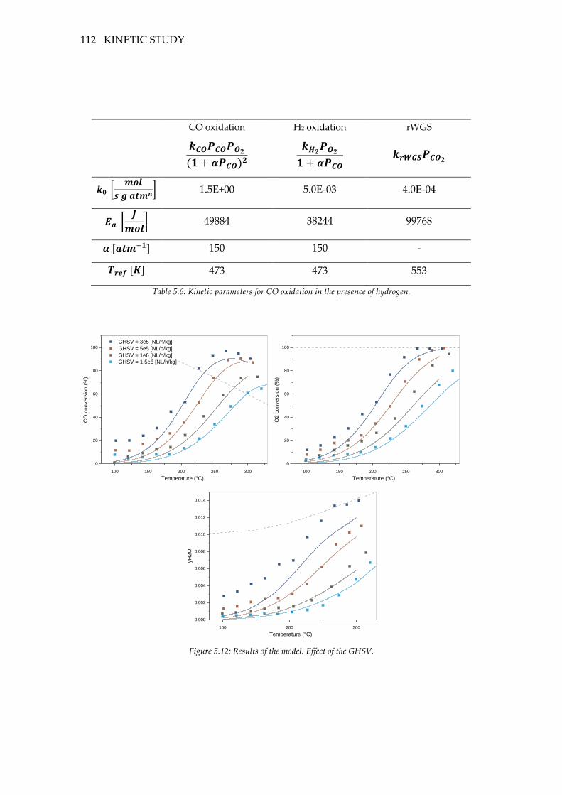
112 KINETIC STUDY
CO oxidation H2 oxidation rWGS
𝒌𝑪𝑶𝑷𝑪𝑶𝑷𝑶𝟐(𝟏 + 𝜶𝑷𝑪𝑶)
𝟐
𝒌𝑯𝟐𝑷𝑶𝟐𝟏 + 𝜶𝑷𝑪𝑶
𝒌𝒓𝑾𝑮𝑺𝑷𝑪𝑶𝟐
𝒌𝟎 [𝒎𝒐𝒍
𝒔𝒈𝒂𝒕𝒎𝒏] 1.5E+00 5.0E-03 4.0E-04
𝑬𝒂 [𝑱
𝒎𝒐𝒍] 49884 38244 99768
𝜶[𝒂𝒕𝒎−𝟏] 150 150 -
𝑻𝒓𝒆𝒇[𝑲] 473 473 553
Table 5.6: Kinetic parameters for CO oxidation in the presence of hydrogen.
100 150 200 250 300
0
20
40
60
80
100
GHSV = 3e5 [NL/h/kg]
GHSV = 5e5 [NL/h/kg]
GHSV = 1e6 [NL/h/kg]
GHSV = 1.5e6 [NL/h/kg]
CO
co
nve
rsio
n (
%)
Temperature (°C) 100 150 200 250 300
0
20
40
60
80
100
O2
co
nve
rsio
n (
%)
Temperature (°C)
100 200 300
0,000
0,002
0,004
0,006
0,008
0,010
0,012
0,014
yH
2O
Temperature (°C)
Figure 5.12: Results of the model. Effect of the GHSV.
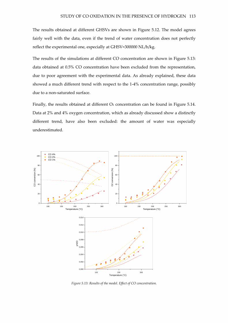
STUDY OF CO OXIDATION IN THE PRESENCE OF HYDROGEN 113
The results obtained at different GHSVs are shown in Figure 5.12. The model agrees
fairly well with the data, even if the trend of water concentration does not perfectly
reflect the experimental one, especially at GHSV=300000 NL/h/kg.
The results of the simulations at different CO concentration are shown in Figure 5.13:
data obtained at 0.5% CO concentration have been excluded from the representation,
due to poor agreement with the experimental data. As already explained, these data
showed a much different trend with respect to the 1-4% concentration range, possibly
due to a non-saturated surface.
Finally, the results obtained at different O2 concentration can be found in Figure 5.14.
Data at 2% and 4% oxygen concentration, which as already discussed show a distinctly
different trend, have also been excluded: the amount of water was especially
underestimated.
100 150 200 250 300
0
20
40
60
80
100 CO 4%
CO 2%
CO 1%
CO
co
nve
rsio
n (
%)
Temperature (°C) 100 150 200 250 300
0
20
40
60
80
100
O2
co
nve
rsio
n (
%)
Temperature (°C)
100 200 300
0,000
0,002
0,004
0,006
0,008
0,010
0,012
0,014
yH
2O
Temperature (°C)
Figure 5.13: Results of the model. Effect of CO concentration.
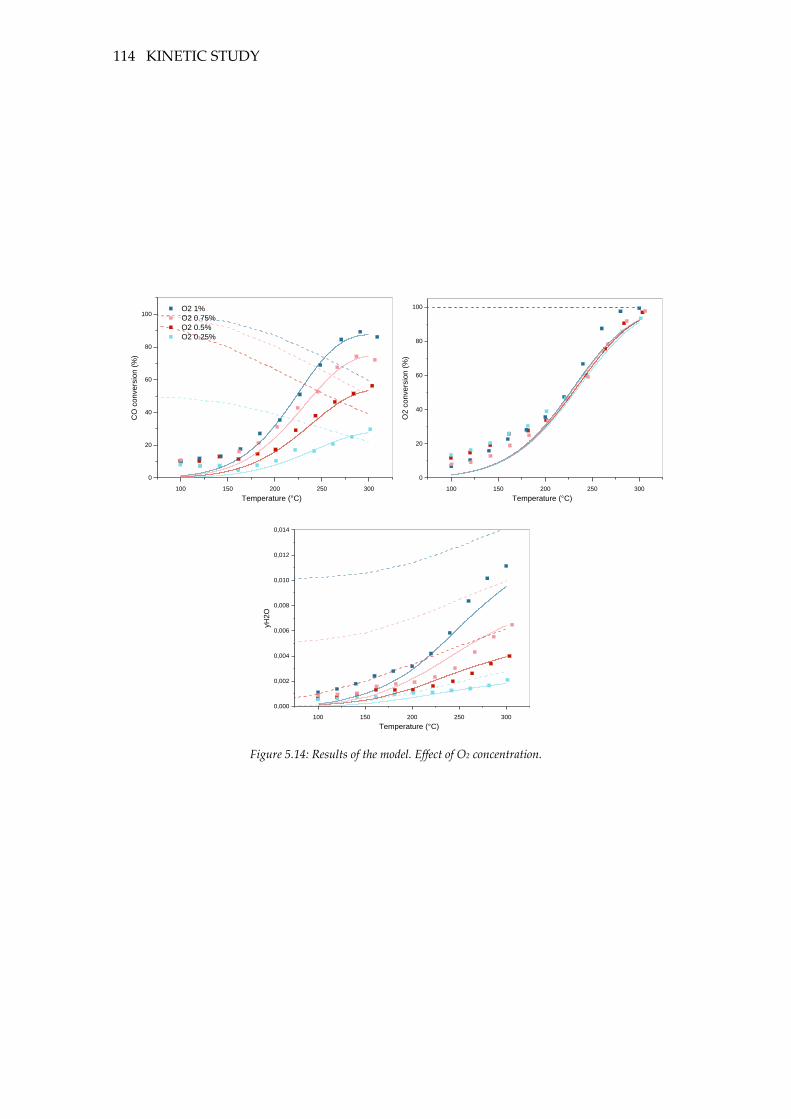
114 KINETIC STUDY
100 150 200 250 300
0
20
40
60
80
100 O2 1%
O2 0.75%
O2 0.5%
O2 0.25%
CO
con
vers
ion
(%
)
Temperature (°C) 100 150 200 250 300
0
20
40
60
80
100
O2
co
nve
rsio
n (
%)
Temperature (°C)
100 150 200 250 300
0,000
0,002
0,004
0,006
0,008
0,010
0,012
0,014
yH
2O
Temperature (°C)
Figure 5.14: Results of the model. Effect of O2 concentration.
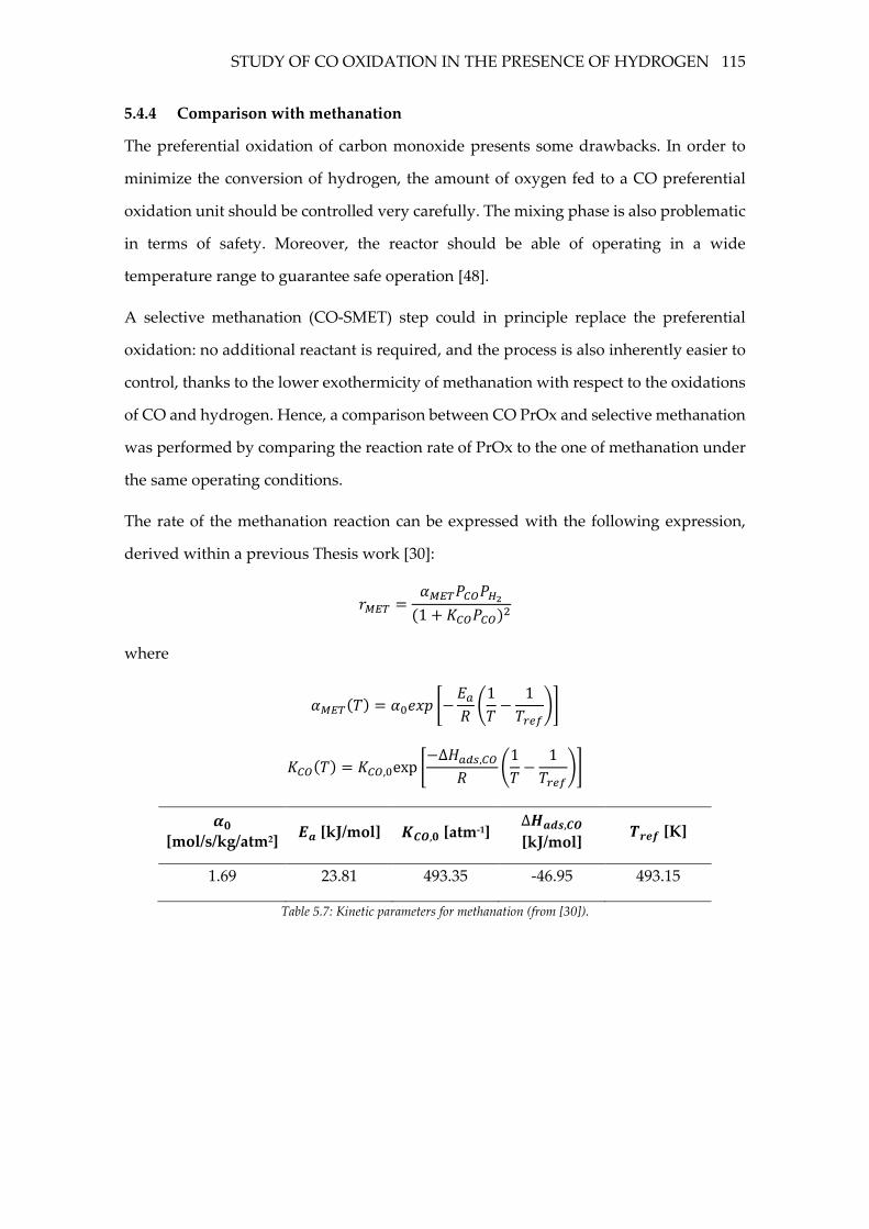
STUDY OF CO OXIDATION IN THE PRESENCE OF HYDROGEN 115
5.4.4 Comparison with methanation
The preferential oxidation of carbon monoxide presents some drawbacks. In order to
minimize the conversion of hydrogen, the amount of oxygen fed to a CO preferential
oxidation unit should be controlled very carefully. The mixing phase is also problematic
in terms of safety. Moreover, the reactor should be able of operating in a wide
temperature range to guarantee safe operation [48].
A selective methanation (CO-SMET) step could in principle replace the preferential
oxidation: no additional reactant is required, and the process is also inherently easier to
control, thanks to the lower exothermicity of methanation with respect to the oxidations
of CO and hydrogen. Hence, a comparison between CO PrOx and selective methanation
was performed by comparing the reaction rate of PrOx to the one of methanation under
the same operating conditions.
The rate of the methanation reaction can be expressed with the following expression,
derived within a previous Thesis work [30]:
𝑟𝑀𝐸𝑇 =𝛼𝑀𝐸𝑇𝑃𝐶𝑂𝑃𝐻2(1 + 𝐾𝐶𝑂𝑃𝐶𝑂)
2
where
𝛼𝑀𝐸𝑇(𝑇) = 𝛼0𝑒𝑥𝑝 [−𝐸𝑎𝑅(1
𝑇−
1
𝑇𝑟𝑒𝑓)]
𝐾𝐶𝑂(𝑇) = 𝐾𝐶𝑂,0exp [−∆𝐻𝑎𝑑𝑠,𝐶𝑂
𝑅(1
𝑇−
1
𝑇𝑟𝑒𝑓)]
𝜶𝟎
[mol/s/kg/atm2] 𝑬𝒂 [kJ/mol] 𝑲𝑪𝑶,𝟎 [atm-1]
∆𝑯𝒂𝒅𝒔,𝑪𝑶
[kJ/mol] 𝑻𝒓𝒆𝒇 [K]
1.69 23.81 493.35 -46.95 493.15
Table 5.7: Kinetic parameters for methanation (from [30]).
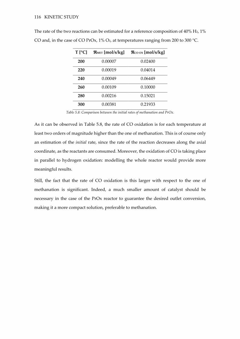
116 KINETIC STUDY
The rate of the two reactions can be estimated for a reference composition of 40% H2, 1%
CO and, in the case of CO PrOx, 1% O2, at temperatures ranging from 200 to 300 °C.
T [°C] ℜMET [mol/s/kg] ℜCO OX [mol/s/kg]
200 0.00007 0.02400
220 0.00019 0.04014
240 0.00049 0.06449
260 0.00109 0.10000
280 0.00216 0.15021
300 0.00381 0.21933
Table 5.8: Comparison between the initial rates of methanation and PrOx.
As it can be observed in Table 5.8, the rate of CO oxidation is for each temperature at
least two orders of magnitude higher than the one of methanation. This is of course only
an estimation of the initial rate, since the rate of the reaction decreases along the axial
coordinate, as the reactants are consumed. Moreover, the oxidation of CO is taking place
in parallel to hydrogen oxidation: modelling the whole reactor would provide more
meaningful results.
Still, the fact that the rate of CO oxidation is this larger with respect to the one of
methanation is significant. Indeed, a much smaller amount of catalyst should be
necessary in the case of the PrOx reactor to guarantee the desired outlet conversion,
making it a more compact solution, preferable to methanation.
117
CONCLUSIONS
The thorough removal of carbon monoxide is a critical issue in hydrogen-rich streams
fed to PEM fuel cells. Indeed, the presence of even small amounts of this species is
associated to efficiency loss and irreversible damage of the Pt anode due to CO-induced
poisoning. The reaction of preferential oxidation of CO (CO PrOx), long-established at
the industrial scale, is vastly employed for this purpose.
A kinetic study of the preferential oxidation reaction was carried out within this Thesis
work, both through experiments at the laboratory scale, and through a modelling phase.
The experiments were initially performed in a diluted packed bed reactor, by using the
catalyst in the form of a powder. Due to issues related to the exothermicity of the
reaction, the dilution ratio was increased more times. Still, radial temperature gradients
were likely affecting the results, according to Mears’ criteria on interparticle heat
transport limitations. This led to the choice of an alternative reactor configuration.
An annular reactor was used to carry out an in-depth kinetic study of CO PrOx. This
type of reactor is particularly indicated for fast, exothermic reactions, thanks to the
additional paths for heat dispersion and the possibility of operating at high space
velocities in the absence of pressure drops. Moreover, it allows to monitor the axial
temperature profile, and to check whether the reaction is actually taking place under
quasi-isothermal conditions.
The effect of different process parameters (space velocity, concentration of CO,
concentration of oxygen) was investigated in the annular system. Tests in the absence of
hydrogen were also performed, in order to evaluate its effect on the kinetics of CO
oxidation. As it was observed, hydrogen has on the one hand a negative impact on the
selectivity, but on the other hand it strongly enhances the reactivity of CO at low
temperatures. This is also proven by the decrease in the apparent activation energy of
the reaction in the presence of hydrogen.
During the experiments, the catalyst showed a very slow, but perfectly reversible
deactivation. In particular, the conversion of both CO and oxygen decreased with the
time on stream. This phenomenon is possibly related to the gradual covering of the
118 CONCLUSIONS
surface by carbon monoxide, producing a poisoning effect on the reactions. As CO
occupies more and more active sites, the adsorption of oxygen is hindered and so is the
oxidation of both CO and hydrogen.
The experimental results clearly showed that both the oxidations are inhibited by CO,
and are on the contrary favoured by large oxygen concentrations. Starting from these
qualitative considerations, simple rate expressions were developed for CO oxidation
(both in the presence and in the absence of hydrogen) and hydrogen oxidation. The
reverse water gas shift reaction, which takes place at high temperatures as oxygen is
depleted, was also added to the kinetic scheme. The parameters for the rate expressions
were obtained by comparing the experimental data to the results of a previously
developed 1-d heterogeneous model for the annular reactor.
The obtained rate expressions can be used for the simulation of a PrOx reactor. A
preliminary comparison with the estimated rate for CO methanation over a Rh catalyst
suggests that the removal of the residual amount of carbon monoxide through
preferential oxidation can be obtained by means of a smaller amount of catalyst and
larger GHSVs than in the case of hydrogenation to CH4.

119
120
BIBLIOGRAPHY
[1] A. Beretta, G. Groppi, C. Ribani, G. Fares and C. Tregambe, "Development of a
Catalytic Fuel Processor for a 10 kW Combined Heat and Power System:
Experimental and Modeling Analysis of the Steam Reforming Unit,"
ChemEngineering, 2018.
[2] F. Ullmann, Ullmann's Encyclopedia of Industrial Chemistry, Wiley-VCH.
[3] J. D. Holladay, J. Hu, D. L. King and Y. Wang, An overview of hydrogen production
technologies, 2009.
[4] A. F. Ghenciu, "Review of fuel processing catalysts for hydrogen production in
PEM fuel cell systems," Current Opinion in Solid State and Materials Science, 2002.
[5] R. Farrauto, Y. Liu, W. Ruettinger, O. Ilinich, L. Shore and T. Giroux, "Precious
metal catalysts supported on ceramic and metal monolithic structures for the
hydrogen economy," Catalysis Reviews - Science and Engineering, 2007.
[6] D. B. Pal, R. Chand, S. N. Upadhyay and P. K. Mishra, Performance of water gas shift
reaction catalysts: A review, 2018.
[7] L. M. Martínez T, O. H. Laguna, C. López-Cartes and M. A. Centeno, "Synthesis
and characterization of Rh/MnO2-CeO2/Al2O3 catalysts for CO-PrOx reaction,"
Molecular Catalysis, 2017.
[8] M. L. Brown, Jr. and A. W. Green, "Treatment Of Gases". Patent 3 088 919, 1963.
[9] F. Romero-Sarria, S. Garcia-Dali, S. Palma, E. M. Jimenez-Barrera, L. Oliviero, P.
Bazin and J. A. Odriozola, "The role of carbon overlayers on Pt-based catalysts for
H2-cleanup by CO-PROX," Surface Science, 2016.
[10] P. C. Hulteberg, J. G. Brandin, F. A. Silversand and M. Lundberg, "Preferential
oxidation of carbon monoxide on mounted and unmounted noble-metal catalysts
in hydrogen-rich streams," International Journal of Hydrogen Energy, 2005.
121
[11] Y. Choi and H. G. Stenger, "Kinetics, simulation and insights for CO selective
oxidation in fuel cell applications," Journal of Power Sources, 2004.
[12] K. Liu, A. Wang and T. Zhang, Recent advances in preferential oxidation of co reaction
over platinum group metal catalysts, 2012.
[13] Y. F. Han, M. J. Kahlich, M. Kinne and R. J. Behm, "CO removal from realistic
methanol reformate via preferential oxidation - Performance of a Rh/MgO catalyst
and comparison to Ru/γ-Al 2O3, and Pt/γ-Al2O3," Applied Catalysis B:
Environmental, 2004.
[14] F. Mariño, C. Descorme and D. Duprez, "Noble metal catalysts for the preferential
oxidation of carbon monoxide in the presence of hydrogen (PROX)," Applied
Catalysis B: Environmental, 2004.
[15] O. Korotkikh and R. Farrauto, "Selective catalytic oxidation of CO in H2: Fuel cell
applications," Catalysis Today, 2000.
[16] A. Sirijaruphan, J. G. Goodwin and R. W. Rice, "Effect of Fe promotion on the
surface reaction parameters of Pt/γ-Al2O3 for the selective oxidation of CO,"
Journal of Catalysis, 2004.
[17] X. Liu, O. Korotkikh and R. Farrauto, "Selective catalytic oxidation of CO in H2:
Structural study of Fe oxide-promoted Pt/alumina catalyst," Applied Catalysis A:
General, 2002.
[18] C. Pedrero, T. Waku and E. Iglesia, "Oxidation of CO in H2-CO mixtures catalyzed
by platinum: Alkali effects on rates and selectivity," Journal of Catalysis, 2005.
[19] M. S. Moreno, E. López, M. E. Adrover, N. J. Divins and J. Llorca, "CO-PrOx over
nano-Au/TiO2: Monolithic catalyst performance and empirical kinetic model
fitting," International Journal of Hydrogen Energy, 2016.
[20] H. C. Lee and D. H. Kim, "Kinetics of CO and H2 oxidation over CuO-CeO2 catalyst
in H2 mixtures with CO2 and H2O," Catalysis Today, 2008.
122
[21] G. Avgouropoulos, T. Ioannides, C. Papadopoulou, J. Batista, S. Hocevar and H. K.
Matralis, "A comparative study of Pt/γ-Al2O3, Au/α-Fe2O3 and CuO-CeO2
catalysts for the selective oxidation of carbon monoxide in excess hydrogen," in
Catalysis Today, 2002.
[22] M. J. Kahlich, H. A. Gasteiger and R. J. Behm, "Kinetics of the selective CO oxidation
in H2-rich gas on Pt/Al2O3," Journal of Catalysis, 1997.
[23] D. H. Kim and M. S. Lim, "Kinetics of selective CO oxidation in hydrogen-rich
mixtures on Pt/alumina catalysts," Applied Catalysis A: General, 2002.
[24] E. J. Bissett, S. H. Oh and R. M. Sinkevitch, "Pt surface kinetics for a PrOx reactor
for fuel cell feedstream processing," Chemical Engineering Science, vol. 60, no. 17, pp.
4709-4721, 9 2005.
[25] W. Hauptmann, M. Votsmeier, H. Vogel and D. G. Vlachos, "Modeling the
simultaneous oxidation of CO and H2 on Pt - Promoting effect of H2 on the CO-
light-off," Applied Catalysis A: General, 2011.
[26] S. Salomons, R. E. Hayes and M. Votsmeier, "The promotion of carbon monoxide
oxidation by hydrogen on supported platinum catalyst," Applied Catalysis A:
General, 2009.
[27] S. Salomons, M. Votsmeier, R. E. Hayes, A. Drochner, H. Vogel and J. Gieshof, "CO
and H2 oxidation on a platinum monolith diesel oxidation catalyst," Catalysis Today,
2006.
[28] M. M. Schubert, M. J. Kahlich, H. A. Gasteiger and R. J. Behm, "Correlation between
CO surface coverage and selectivity/kinetics for the preferential CO oxidation over
Pt/γ-Al2O3 and Au/α-Fe2O3: an in-situ DRIFTS study," 1999.
[29] A. B. Mhadeshwar and D. G. Vlachos, "Hierarchical, multiscale surface reaction
mechanism development: CO and H2 oxidation, water-gas shift, and preferential
oxidation of CO on Rh," Journal of Catalysis, 2005.
[30] R. Rinaldi and V. Troisi, "Small scale fuel processing: a kinetic investigation of CO
methanation," Politecnico di Milano, 2018.
123
[31] C. Cristiani, M. Valentini, M. Merazzi, S. Neglia and P. Forzatti, "Effect of ageing
time on chemical and rheological evolution in γ-Al2O3 slurries for dip-coating," in
Catalysis Today, 2005.
[32] A. G. Bayram and V. Piazza, "Syngas production from ethanol and formic acid over
Rh/Al2O3: a kinetic study in annular reactor," Politecnico di Milano, 2019.
[33] Colorado State University, "Chemical Equilibrium Calculator," [Online]. Available:
http://navier.engr.colostate.edu/code/code-4/index.html.
[34] R. Rota, Fondamenti di termodinamica dell'ingegneria chimica, Pitagora Editrice,
2015.
[35] J. Pérez-Ramírez, R. J. Berger, G. Mul, F. Kapteijn and J. A. Moulijn, "Six-flow
reactor technology a review on fast catalyst screening and kinetic studies," Catalysis
Today, 2000.
[36] A. Beretta, G. Groppi, L. Majocchi and P. Forzatti, "Potentialities and draw-backs
of the experimental approach to the study of high T and high GHSV kinetics,"
Applied Catalysis A: General, 1999.
[37] C. Beniani, "Experimental and modelling analysis of the water gas shift reactor in
a combined heat and power unit," Politecnico di Milano, 2018.
[38] R. H. Nibbelke, M. A. Campman, J. H. Hoebink and G. B. Marin, "Kinetic study of
the CO oxidation over Pt/γ-Al2O3 and Pt/Rh/CeO2/γ-Al2O3 in the presence of
H2O and CO2," Journal of Catalysis, 1997.
[39] A. Sirijaruphan, J. G. Goodwin and R. W. Rice, "Investigation of the initial rapid
deactivation of platinum catalysts during the selective oxidation of carbon
monoxide," Journal of Catalysis, vol. 221, no. 2, pp. 288-293, 25 1 2004.
[40] D. E. Mears, "Tests for Transport Limitations in Experimental Catalytic Reactors,"
Industrial and Engineering Chemistry Process Design and Development, 1971.
[41] "EUROKIN spreadsheet on requirements for measurement of intrinsic kinetics in
the gas-solid fixed-bed reactor," 2012. [Online]. Available:
124
https://www.eurokin.org/wp-content/uploads/webtool/EUROKIN_fixed-
bed_html.htm.
[42] "ASALI - CatalyticFOAM," [Online]. Available:
http://www.catalyticfoam.polimi.it/asali-2/.
[43] A. Beretta, P. Baiardi, D. Prina and P. Forzatti, "Analysis of a catalytic annular
reactor for very short contact times," Chemical Engineering Science, 1999.
[44] G. F. Froment, K. B. Bischoff and J. De Wilde, Chemical Reactor Analysis and
Design - 3rd Ed., Wiley, 2011.
[45] A. Donazzi, A. Beretta, G. Groppi and P. Forzatti, "Catalytic partial oxidation of
methane over a 4% Rh/α-Al2O3 catalyst. Part I: Kinetic study in annular reactor,"
Journal of Catalysis, 2008.
[46] B. W. Wojciechowski and S. P. Asprey, "Kinetic studies using temperature-
scanning: The oxidation of carbon monoxide," Applied Catalysis A: General, 2000.
[47] A. Bourane, O. Dulaurent and D. Bianchi, "Heats of adsorption of linear and
multibound adsorbed CO species on a Pt/Al2O3 catalyst using in situ infrared
spectroscopy under adsorption equilibrium," Journal of Catalysis, 2000.
[48] M. A. Ashraf, G. Ercolino, S. Specchia and V. Specchia, "Final step for CO syngas
clean-up: Comparison between CO-PROX and CO-SMET processes," in
International Journal of Hydrogen Energy, 2014.