SMS 11.1 Tutorial TUFLOW 1D/2D

Objectives This tutorial describes the generation of a 1D TUFLOW project using the SMS interface. It is recommended that the TUFLOW 2D tutorial be done before doing this tutorial. TUFLOW is a hydraulic model that can work with mixed 1D/2D solutions. It handles wetting and drying in a very stable manner. More information about TUFLOW can be obtained from the TUFLOW website: www.TUFLOW.com. The area used in the tutorial is where the Cimarron River crosses I-35 in Oklahoma, about 50 miles North of Oklahoma City.

Prerequisites • TUFLOW 2D Tutorial

Requirements • Map Module • Grid Module • Scatter Module • Grid Module

Time • 60-75 minutes

v. 11.1

1 Background Data

This tutorial focuses on adding 1D cross-sections to a 2D model. We will start with the grid as created in the 2D TUFLOW tutorial. Refer to that tutorial to learn how to setup the grid. The modeling process when using combined 1D and 2D components with the TUFLOW model includes the following:

• Defining the 2D domain or active portion of the grid.

• Specifying the 1D network (center line and cross sections).

• Defining the 1D/2D connections

• Specifying the boundary conditions

• Combining all the components into a simulation.

A TUFLOW model uses grids to define the two dimensional (Eulerian) domain. It uses GIS objects grouped in what SMS refers to as feature coverages to define modifications to the grid such as levies or embankments. Feature objects can also be used to define additional objects such as cross sections and channel centerlines. A TUFLOW simulation consists of a group of these geometrical objects, along with model parameters and specifications. Note that all units in TUFLOW must be metric. We are going to build a model that uses a 1D cross-section based solution within the channel and 2D cell-based solution outside the channel. A 1D/2D model gives better channel definition than an all 2D model because the cross sections have higher resolution than the 2D grid allows. Additionally, a 1D/2D model generally has a shorter computation time.

To start the tutorial:

1. Click File | Open and find the file Cimmaron_1D.sms This will load an SMS project with a background image, the elevation data in a TIN, the 20m grid created in the 2D tutorial, and three map coverages. The coverages include the material zones defined in an area properties coverage, a pre-digitized boundary of the channel or 1D area, and separate coverage with defined locations for cross sections. SMS should look like Figure 1.

Figure 1 View of Map and Image Data

2 1D/2D TUFLOW models

TUFLOW supports several methods for linking 1D and 2D models as described in the TUFLOW reference manual, including:

• Embedding a 2D domain inside of a large 1D domain (see sketch 1a in Figure 2).

• Insert 1D networks “underneath” a 2D domain (see sketch 1b in Figure 2 and Figure 3).

• Replace or “carve” a 1D channel through a 2D domain (see sketch 1c in Figure 2 and Figure 4).

This tutorial illustrates the third application.

1D Network 1D Network 2D

1D boundary condition

Small 1D elements representing culverts

1D boundary condition

1a

1b

1c

1D representation of open channel

2D

Small 1D elements representing culverts

1D representation of pipe network

Figure 2 Various methodologies to link 1D and 2D domains (From TUFLOW Users

Manual - www.TUFLOW.com)

1D

2D

Figure 3 Pipe network underneath a 2D model (From TUFLOW Users Manual -

www.TUFLOW.com)

1D

2D 2D

Figure 4 Open Channel (1D) within a 2D domain(From TUFLOW Users Manual -

www.TUFLOW.com)

3 Defining the 2D portion of the model

The TUFLOW 2D tutorial demonstrates how to define a grid to represent the geographical features in a study domain such as a flood plain. The combined 1D/2D simulation continues to utilize this grid. However, portions of the grid are disabled or eliminated because that portion of the simulation will be represented with a 1D network. The user must define these portions.

3.1 2D Computation Domain

For this tutorial, the region that should not be included in the 2D calculations has already been defined in the "Channel Boundary" coverage.

1. Click on the " Channel Boundary” coverage to display this polygon.

2. Note that the orange polygon encloses the channel and the regions both upstream and down stream from the study area. The area in this polygon will be simulated using 1D analysis.

We need to specify that this polygon is not to be included in the 2D calculations. To do this, we assign an attribute to the polygon. The steps are:

1. Right Click on the coverage named “Channel Boundary”. In the pop up menu that appears, select "Type". This will bring up a second menu. Select "Models" which will bring up a list of models your license of SMS includes. In this list select "TUFLOW" to see the list of TUFLOW coverages. In this menu, select TUFLOW | 1D/2D BCs and Links. to specify the coverage type.

2. Select the Select Feature Polygon tool and double click inside the channel. The Boundary Conditions dialog appears

3. Set the "Type" to No BC and toggle on the Set cell code. Set the "Code" to Inactive -- not in mesh. When using this option, TUFLOW will not create 2D cells in this area. (The dialog is shown in Figure 5.)

Figure 5 BC Polygon Attributes Dialog

4. Click OK to exit the dialog

4 Setting up the 1D Network

Several coverages are used to define the 1D cross-section based network. The first coverage we will create will be of type “TUFLOW 1D Network.” This coverage will be used to define the centerline for the channels as well as the attributes for the weir. To speed the process of creating the network, and to maintain consistency with the contents of this document, the channel points have been given. To create the channels:

1. To reduce the amount of data you are dealing with on the screen, uncheck the box next to the "20m" grid in the Project Explorer to turn of the grid display.

2. Click on the coverage named “1D Network” to make it active. You will notice that we have digitized several points down the channel to facilitate the process and keep your work consistent with the contents of this tutorial. In your project, you would digitize with guidance from the underlying image or topographic data.

3. Right click on the coverage and change the type to Models | TUFLOW | 1D Networks similar to how you specified the type of the “Channel Boundary” coverage in the previous section.

4. Using the Create Feature Arc tool, create a series of arcs (one for each node pair). This means that the arc will start and stop at each node. By default, each arc represents a segment of open channel. The length of an arc should come from the channel it is representing. Each arc should represent a fairly consistent cross section shape. Feel free to add intermediate vertices to make the centerline smoother. You may want to zoom in and pan along the channel as you define the arcs. The finished digitized arcs should look something like Figure 6.

Figure 6 Creating the 1D Network centerline

Now that the channel centerline is defined, we need to specify that the most upstream arc represents a weir. A weir will get the flow into the model and spread the flow into both the 1D and 2D domains. We will create a wide weir which will receive the inflow and then it will be distributed between the 1D and 2D domains downstream.

1. Using the Select Feature Arc tool select the first arc in the network.

2. Right click and select Attributes.

3. Change the type to Weir and click on the button labeled Attributes at the bottom of the dialog. The dialog should look like Figure 7.

Figure 7 Channel Attributes Dialog

4. Set the Invert to 264 meters (this value comes from the elevation data for the channel) and the Width to 1000 meters (this is wide enough to cover the majority of the floodplain). Make sure the dialog looks like Figure 8 and Click “OK” twice to exit the dialogs.

Figure 8 Values for Weir Attributes

4.1 Creating Cross Sections

Each open channel arc uses cross-section geometry to compute hydraulic properties (such as area and wetted perimeter) for each channel segment. TUFLOW needs to have a geometric definition for the channel for each segment as well as invert elevations at the cross section end points. The invert elevations define channel slope. Cross-sections can be defined in the middle of a channel or at the channel endpoints or both. If cross-sections are specified at the endpoints the cross-section information used for each channel is averaged from the cross-section at each end and TUFLOW extracts the channel inverts from the cross section definitions. If cross-sections are specified at the middle of the channel segment, the upstream and downstream inverts must be specified manually. If cross-sections exist at both the endpoints and within the channel, the cross-section properties are taken from the cross-section within the channel and the inverts from the cross-sections at the ends. For this tutorial, we will create cross-sections at the end of each channel. We will layout cross-sections from the channel segments in the network coverage and then trim them to the edge of our 1D domain, all using tools in SMS. Once the cross-sections have been defined, we will extract elevations for them from the elevation data in our TIN and material data from the area property coverage.

To layout and trim the cross-sections.

1. Right click on “Map Data” and click on New Coverage.

2. Make the new coverage a TUFLOW | 1D Cross Sections Coverage and name it “Cross Sections”. Click OK.

3. The CsDb Management dialog will pop up. Click OK to close it.

4. Go to Display | Display Options. Make sure that Map is selected and turn on the Inactive coverage toggle. Click OK.

5. In the Project Explorer, turn off the materials coverage, the grid, the survey, and the image. Working only with the feature 1D network data will be more clear.

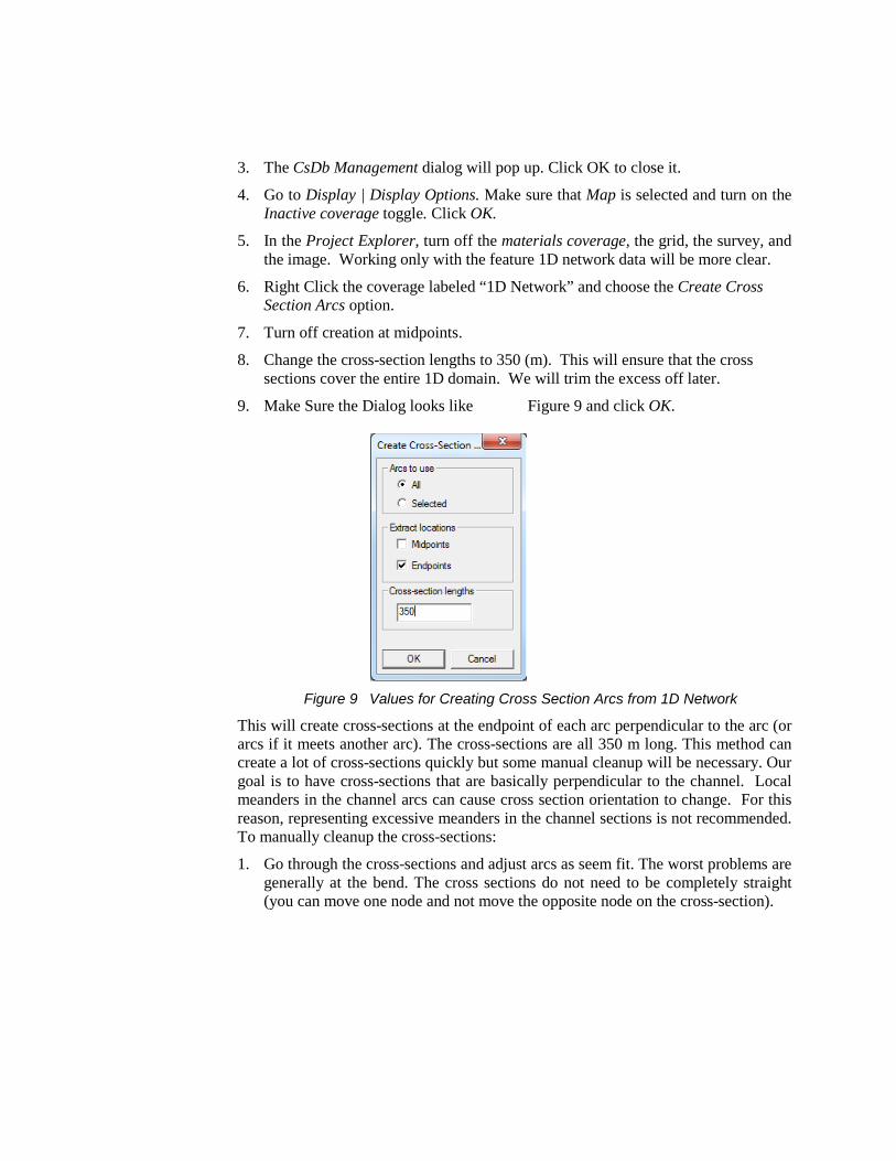
6. Right Click the coverage labeled “1D Network” and choose the Create Cross Section Arcs option.

7. Turn off creation at midpoints.

8. Change the cross-section lengths to 350 (m). This will ensure that the cross sections cover the entire 1D domain. We will trim the excess off later.

9. Make Sure the Dialog looks like Figure 9 and click OK.

Figure 9 Values for Creating Cross Section Arcs from 1D Network

This will create cross-sections at the endpoint of each arc perpendicular to the arc (or arcs if it meets another arc). The cross-sections are all 350 m long. This method can create a lot of cross-sections quickly but some manual cleanup will be necessary. Our goal is to have cross-sections that are basically perpendicular to the channel. Local meanders in the channel arcs can cause cross section orientation to change. For this reason, representing excessive meanders in the channel sections is not recommended. To manually cleanup the cross-sections:

1. Go through the cross-sections and adjust arcs as seem fit. The worst problems are generally at the bend. The cross sections do not need to be completely straight (you can move one node and not move the opposite node on the cross-section).

2. The very first channel is our weir and so we don’t need the cross-section at the first node. Delete it.

3. The first and the last cross-sections should connect with the extents of the 2D domain. Drag the endpoints of these arcs to the nodes in the "Channel Boundary" coverage. You should see a red x as you get close to the point indicating that the point will snap to the existing node location.

All of the cross-sections that we generated (except for the couple we moved already) extend outside of the 1D channel boundary. We only want cross-sections within the channel area. To trim the cross-sections to the boundary:

1. Right click the coverage labeled “Cross Sections” and choose the Trim to Code Polygon option. This will trim the cross-sections to the code polygons in a boundary condition coverage. Since we only have one boundary condition coverage, it will be used automatically. (If you are working with a project that uses more than one such coverage, a dialog will appear to choose a coverage.) When you are done the cross sections should look like Figure 10.

Figure 10 Final Trimmed Cross Section Arcs

Now that the cross-sections are laid out and trimmed, we need to extract elevation and material data. To extract this information and verify that it is setup:

1. Right click on the Cross Sections coverage and select Extract from Scatter. This will extract elevation data from the active dataset on the active scatter set (TIN).

2. Right click on the “Cross Sections” coverage again and select Map Materials From Area Coverage. This will map materials from an area property coverage. In the Select Coverage dialog, Select materials and set the Default material to channel. (If more than one area property coverage exists, the coverage to use can be selected.) Click OK.

We now have cross-sections with elevation and material information. We can view/edit the data used for each cross-section using the cross-section editor in SMS.

1. Click the Select Feature Arc tool and double click on one of the cross section arcs. A dialog appears showing the cross section ID.

2. Click on the Edit button and the cross section attributes dialog appears.

3. This dialog includes a plot of the cross-section with several tools to edit the cross-section data. Figure 11 is an example of the dialog. In the Geom Edit tab, you can edit the coordinates which define the cross-section. The edits can be done graphically in the plot or by editing the spreadsheet. The x, and y coordinates represent the location of the cross-section in plan view and are ignored by TUFLOW. The d value is the distance along the cross-section from the left bank towards the right bank. The z value is the elevation of the point.

Figure 11 Cross Section Attributes Dialog

4. If you click on the Line Props tab, you can view the materials that are assigned to each section of the Cross Section. The material breaks may be edited in this dialog using the tools in the plot window or the spreadsheet below.

5. If you had additional information that you want to incorporate into the cross section you would do it here. Since we don't have additional data, click Cancel twice to return to the main screen.

Another useful tool to see cross sections is the TUFLOW Cross-section plot. With this tool several different cross sections can be selected and viewed at the same time.

1. Select Display | Plot Wizard…

2. Select TUFLOW Cross Section and click Finish.

3. Now select a cross section with the Select Feature Arc tool. The Cross Section profile will appear in “Plot 1.”

4. Holding Shift select several other cross sections. The last arc selected will be in blue while the other arcs will be in green. This way you can compare how each cross sections compares to others as in Figure 12.

Figure 12 TUFLOW Cross Section Plot

Click on the X at the upper right corner of the plot window when you are done reviewing the plots.

5 Defining the 1D/2D Connection We have to tell TUFLOW where flow will be allowed to move between the 1D and 2D domains. The main flow exchanges will be along both banks of the channel. At the top of the model, all flow will enter a wide 1D domain and then the flow will be split into the 1D domain for the channel flow and into the 2D domain for the floodplain flow.

5.1 1D/2D Flow Interfaces The locations for flow exchange are named 1D flow/2D water level connections in the SMS interface or HX lines. These will be referred to as HX arcs throughout the remainder of this tutorial. The first type of location where this transition will take place

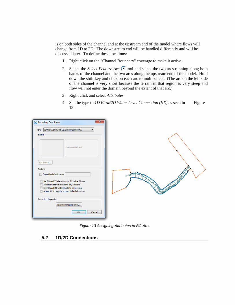
is on both sides of the channel and at the upstream end of the model where flows will change from 1D to 2D. The downstream end will be handled differently and will be discussed later. To define these locations:

1. Right click on the "Channel Boundary" coverage to make it active.

2. Select the Select Feature Arc tool and select the two arcs running along both banks of the channel and the two arcs along the upstream end of the model. Hold down the shift key and click on each arc to multi-select. (The arc on the left side of the channel is very short because the terrain in that region is very steep and flow will not enter the domain beyond the extent of that arc.)

3. Right click and select Attributes.

4. Set the type to 1D Flow/2D Water Level Connection (HX) as seen in Figure 13.

Figure 13 Assigning Attributes to BC Arcs

5.2 1D/2D Connections

There are two parts to defining 1D/2D links. The first is on the 2D domain, and the second is in the 1D domain. We have already defined the flow interfaces between the 1D and 2D domains in the "Channel Boundary" coverage. TUFLOW associates these arcs with the 2D domain spatially. Along with these HX arcs, we must define the 1D/2D connection from the 1D network nodes. These 1D/2D connection arcs tell TUFLOW which locations along the HX arcs match individual nodes. Since the cross-section arcs are in the same locations as we want to place our 1D/2D connections, we will start with a copy of the cross section coverage.

1. Right click the “Cross Section” coverage and select Duplicate. This creates a coverage named "Copy of Cross Sections".

2. Click on the new coverage to make it active, then right click on it and rename it to “1D_2D_Connection”.

3. Right click again and change the type to TUFLOW | 1D/2D Connections.

4. Using the Select Feature Vertex tool right click in an area where nothing is and select Select All. This will select all of the vertices. There is one vertex at the center of each cross section.

5. Right click again and select the Convert to Nodes option. This splits each of the arcs into two arcs and now we have separate arcs connecting each node on the centerline to the HX arcs.

6. Right click on the 1D_2D_Connection Coverage and select Properties. Select Channel Boundary as the TUFLOW boundary condition to use with the 1D_2D_Connection coverage. Click OK.

Figure 14 Vertices along 1D/2D Connection arcs which will be converted to nodes

7. TUFLOW requires that the HX arcs (in the "Channel Boundary" coverage) have a vertex at each 1D/2D connection point. SMS can enforce this. Right click on the “1D_2D_Connection” coverage and select Clean Connections. This brings up the Clean Options dialog.

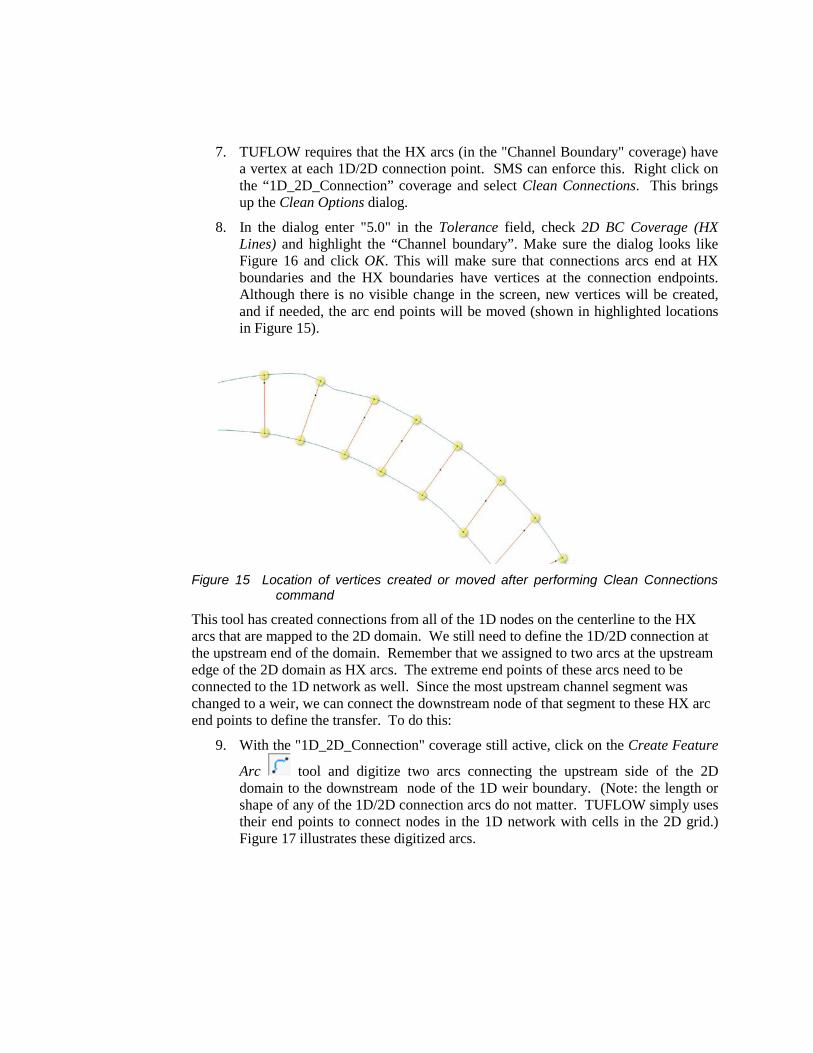
8. In the dialog enter "5.0" in the Tolerance field, check 2D BC Coverage (HX Lines) and highlight the “Channel boundary”. Make sure the dialog looks like Figure 16 and click OK. This will make sure that connections arcs end at HX boundaries and the HX boundaries have vertices at the connection endpoints. Although there is no visible change in the screen, new vertices will be created, and if needed, the arc end points will be moved (shown in highlighted locations in Figure 15).

Figure 15 Location of vertices created or moved after performing Clean Connections

command

This tool has created connections from all of the 1D nodes on the centerline to the HX arcs that are mapped to the 2D domain. We still need to define the 1D/2D connection at the upstream end of the domain. Remember that we assigned to two arcs at the upstream edge of the 2D domain as HX arcs. The extreme end points of these arcs need to be connected to the 1D network as well. Since the most upstream channel segment was changed to a weir, we can connect the downstream node of that segment to these HX arc end points to define the transfer. To do this:

9. With the "1D_2D_Connection" coverage still active, click on the Create Feature

Arc tool and digitize two arcs connecting the upstream side of the 2D domain to the downstream node of the 1D weir boundary. (Note: the length or shape of any of the 1D/2D connection arcs do not matter. TUFLOW simply uses their end points to connect nodes in the 1D network with cells in the 2D grid.) Figure 17 illustrates these digitized arcs.

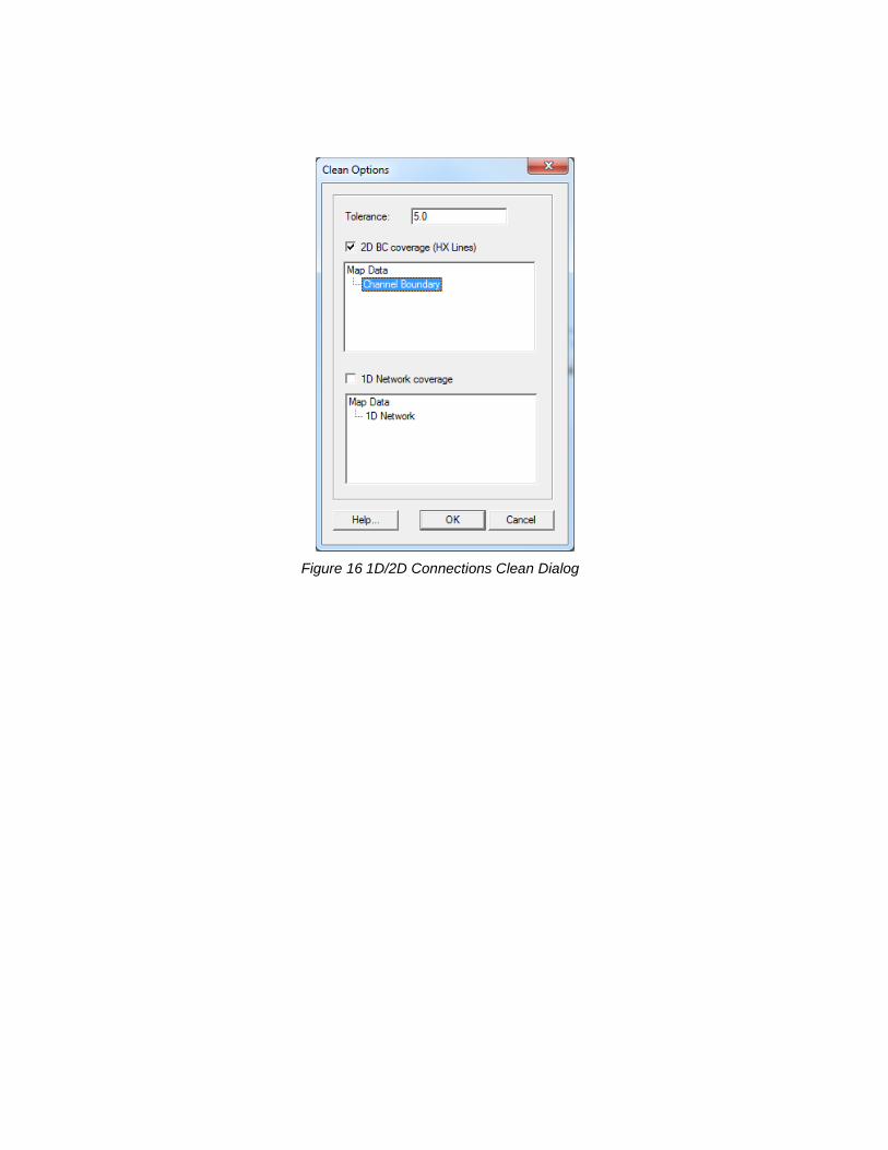
Figure 16 1D/2D Connections Clean Dialog

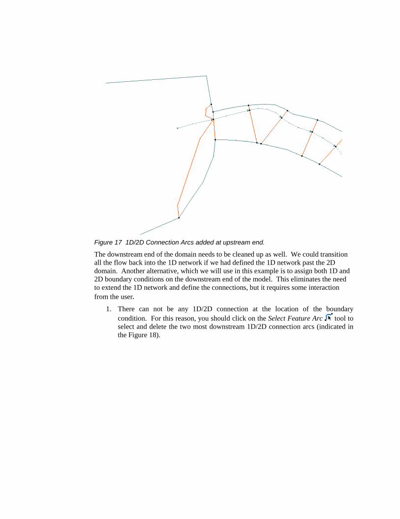
Figure 17 1D/2D Connection Arcs added at upstream end.

The downstream end of the domain needs to be cleaned up as well. We could transition all the flow back into the 1D network if we had defined the 1D network past the 2D domain. Another alternative, which we will use in this example is to assign both 1D and 2D boundary conditions on the downstream end of the model. This eliminates the need to extend the 1D network and define the connections, but it requires some interaction from the user.

1. There can not be any 1D/2D connection at the location of the boundary condition. For this reason, you should click on the Select Feature Arc tool to select and delete the two most downstream 1D/2D connection arcs (indicated in the Figure 18).

Figure 18 Location of deleted 1D/2D connection arcs on downstream end.

(Note: if you examine the HX arcs you created in the previous section, you will note that they end one cross section above the end of the 1D network. This was done to prevent an illegal 1D/2D connection at the boundary condition. The connection arcs you just deleted actually didn't connect to an HX arcs for this reason. This is a limitation of the 1D/2D boundary condition. There will be no transfer of flow between the 1D network and the 2D grid in this last channel segment.)\

6 Specifying the boundary conditions As with any numerical model, we need to specify the boundary conditions. This principally defines where the flow enters and leaves the simulation. In this tutorial we will have flow enter the simulation in the 1D network, and leave both the 1D network and the 2D grid. The inflow will be specified as a flow rate over the weir. The outflow will be controlled by specifying a head condition.

6.1 2D Downstream Water Level Boundary Condition On the downstream end of our domain, we are going to assign a water level boundary condition to both the 1D domain and to the 2D domain. Since the 2D domain is split by the 1D domain, there will be 2 water level boundary condition arcs in this coverage.

1. Select the "Channel Boundary" coverage to make it active.

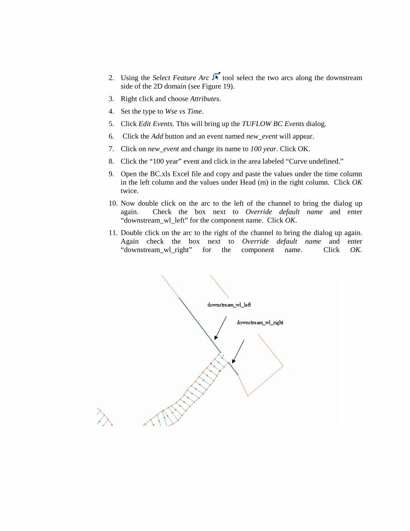
2. Using the Select Feature Arc tool select the two arcs along the downstream side of the 2D domain (see Figure 19).

3. Right click and choose Attributes.

4. Set the type to Wse vs Time.

5. Click Edit Events. This will bring up the TUFLOW BC Events dialog.

6. Click the Add button and an event named new_event will appear.

7. Click on new_event and change its name to 100 year. Click OK.

8. Click the “100 year” event and click in the area labeled “Curve undefined.”

9. Open the BC.xls Excel file and copy and paste the values under the time column in the left column and the values under Head (m) in the right column. Click OK twice.

10. Now double click on the arc to the left of the channel to bring the dialog up again. Check the box next to Override default name and enter “downstream_wl_left” for the component name. Click OK.

11. Double click on the arc to the right of the channel to bring the dialog up again. Again check the box next to Override default name and enter “downstream_wl_right” for the component name. Click OK.

Figure 19: Location of Downstream BC Arcs

6.2 Creating The 1D BC The 1D network needs boundary conditions for both the upstream and downstream boundaries. To define the 1D boundary conditions:

1. Right click Map Data and create a new coverage of type TUFLOW | 1D/2D BC and Links named "1d_bc". Click on this coverage to make it active.

2. Using the Create Feature Point tool, create points directly on top of the first and last nodes in the network coverage. As you get close to the nodes in the other coverage, you should see red cross-hairs. This indicates that the node will snap to the existing node in the other coverage. If you do not see the red cross-hairs, hitting “s” on your keyboard will activate this snapping functionality. (If your simulation is very crowded, you could turn off all the coverages in the project explorer except “1D network” and “1d_bc” so you won’t snap to nodes in other coverages.)

3. Using the Select Feature Point tool, double click the node at the upper end of the river.

4. Change the type to Flow vs Time (QT) and click the Override default name checkbox and type “Upstream_1D”.

5. Choose “100 year” under Events.

6. Click on the curve button (the area labeled “Curve undefined”) and enter the time and flow information found in the excel file bc.xls. Click OK twice to exit the dialog.

7. Now double click the downstream node.

8. Make the type Wse vs Time (HT) and click the Override default name checkbox and type “Downstream_1D”.

9. Choose “100 year” under Events.

10. Click on the curve button and enter the time and water level information from the excel file bc.xls to define the curve (as you did for the 2D boundary condition). Click OK twice to exit the dialog.

7 Creating Water Level Line Coverage for Output TUFLOW can generate output that looks like 2D output from the 1D solution. This becomes part of the output mesh and can be viewed inside of SMS. The mesh node locations in this output are determined by water level lines. The spacing of nodes along the water level lines is specified for each water level line.

1. Right click on the “1D Network” and select Create Water Level Arcs.

2. In the Create Water Level Arcs dialog set the distance between water level arcs to 60.0, set the Arc length to 350.0, and make sure the default point distance is 10.0. Make sure that Create New Coverage is checked. Click OK.

3. Rename the new coverage “Water Level Lines.”

4. Right click the coverage and select “Trim to Code Polygon.”

5. Select “Channel Boundary” in the Select Coverage dialog.

6. Delete any water level lines above the first cross section or below the last cross section.

7. Crosssing water level lines create inverted elements. Look for crossing water level lines at the river bend and towards the bottom end of the model. Delete crossing water level lines or drag their endpoints so they don’t overlap.

8 TUFLOW Simulation A TUFLOW simulation is comprised of a grid, feature coverages, and model parameters. We were given a grid and created several coverages to use in TUFLOW simulations. SMS allows for the creation of multiple simulations each which includes links to these items. The use of links allows these items to be shared between multiple simulations. A simulation also stores the model parameters used by TUFLOW. To create the TUFLOW simulation:

1. Right click in the empty part of the project explorer and choose New Simulation | TUFLOW. This will create several new folders that we will discuss as we go. Under the tree item named Simulations, there will be a new tree item named “Sim.”

2. Rename the sim tree item, “100year_20m.”

8.1 Geometry Components Grids are shared through geometry components as explained in the TUFLOW 2D tutorial. To create and setup the geometry component:

1. Right click on the folder named “Components” and choose New 2D Geometry Component.

2. Rename the new tree item from 2D Geom Component to 20m.

3. Drag under this tree item the grid, and the following coverages: “materials” "1d_bc" and “Channel Boundary”.

8.2 Material Definitions Now that we have a Simulation, we need to define our material properties. There is already a Material Definitions folder but we need to create material definition sets or a set of values for the materials.

1. Right click on the Material Sets folder and select “New Material Set” from the menu. A new Material Set will appear.

2. Right click on the new Material Set in the project explorer and select Properties from the menu. The Materials are displayed in the list box on the left.

3. Change the values for Manning’s n for all the materials according to Table 1. Click OK to accept these values and exit the dialog.

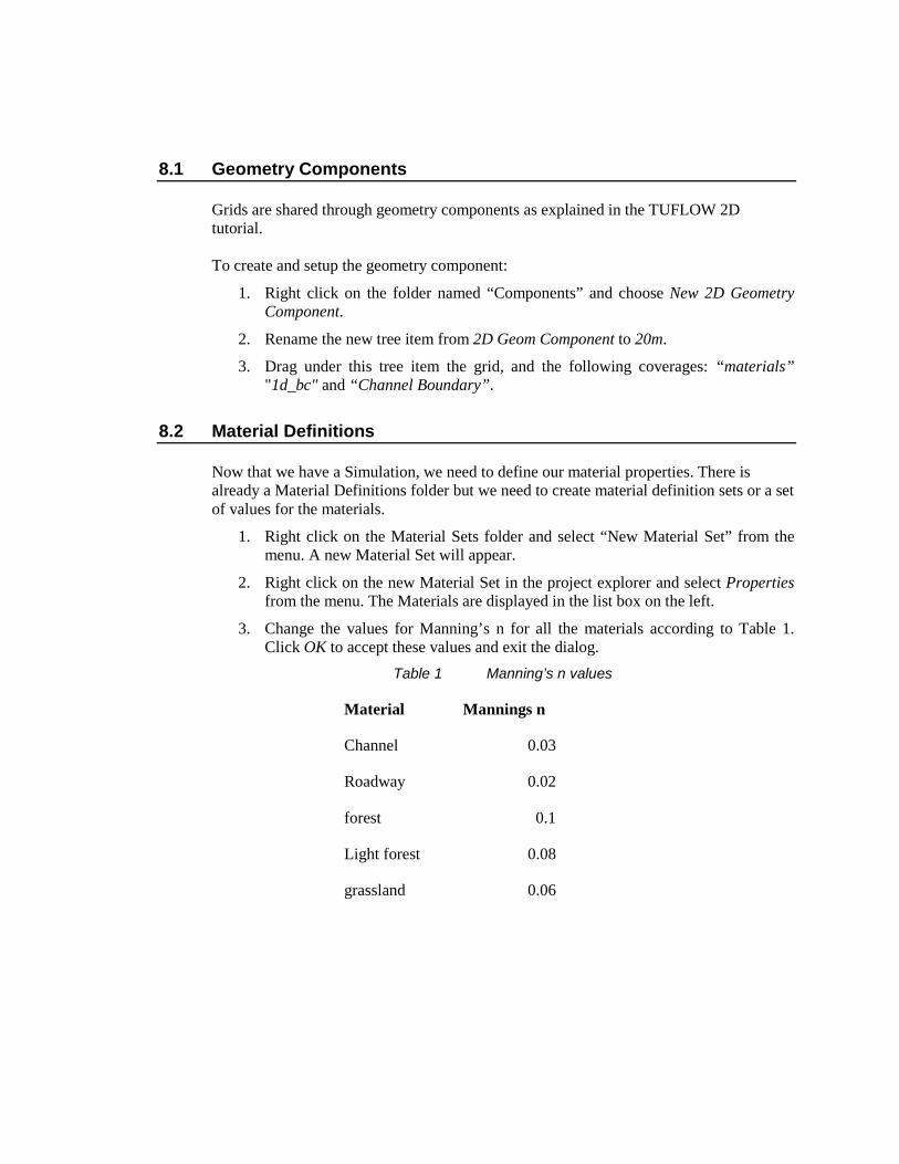
Table 1 Manning’s n values

Material Mannings n

Channel 0.03

Roadway 0.02

forest 0.1

Light forest 0.08

grassland 0.06

8.3 Simulation Setup and Model Parameters We need to add the items which will be used in the simulation. These items include the geometry component and coverages. Coverages already in the geometry component do not need to be added to the simulation. Drag the following items underneath the simulation in the project explorer:

• The geometry component (20m).

• The following coverages: Cross Sections, 1d_bc, 1D Network, Water Level Lines, and 1D_2D Connection.

The TUFLOW model parameters include timing controls, output controls, and various model parameters. To setup the model control parameters:

1. Right click on the 100year_20m simulation and select 2D Model Control. Select the Output Control tab if it is not already selected.

2. In the Map Output section, set the Format type to “SMS 2dm”; the Start Time to 0 hours and the Interval to 900 seconds (15 minutes).

4. In the Output Datasets section, select the following datasets: Depth, Water Level, Flow Vectors (unit flowrate), and Velocity Vectors.

5. In the Screen/Log Output section, change the display interval to 6. While TUFLOW is running, it will write status information every 6 timesteps.

6. Switch to the Time tab. Change the Start Time 2 hours and the End Time to 16 hours. Change the timestep to 5.0 seconds.

7. Switch to the Water Level tab and change the Initial Water Level to 265.5. Turn on Override Default Instability Level and set it to 285.0.

8. Switch to the BC tab and switch the BC Event Name to 100 year.

9. Click OK to close the Model Control dialog.

In addition to the normal model parameters, we need to specify parameters specifically for the 1D portion of the model.

1. Right click again on the 100year_20m simulation and select 1D Control.

2. In the General tab change the Initial Water Level to 265.5, and the output interval to 900 seconds.

3. In the Network tab, change the depth limit factor to 5.0. This allows water in the channels to be up to five times deeper than the depth of the channel before halting due to a detected instability.

4. Click OK to close the Control 1D dialog.

Figure 20 Final View of Project Explorer

9 Saving a Project File To save all this data for use in a later session:

1. Select File | Save New Project.

2. Save the file as Cimaron1d.sms.

3. Click the Save button to save the files.

10 Running TUFLOW TUFLOW can be launched from inside of SMS. Before launching TUFLOW the data in SMS must be exported into TUFLOW files. To export the files and run TUFLOW:

1. Right click on the simulation and select export TUFLOW files. This will create a directory named TUFLOW where the files will be written. The directory structure models that described in the TUFLOW users manual.

2. Right click on the simulation and select Launch TUFLOW. This will bring up a console window and launch TUFLOW.

11 Using Log and Check Files TUFLOW generates several files that can be useful for locating problems in a model. In the TUFLOW directory under \runs\log, there should be a file named 100year_20m.tlf. This is a log file generated by TUFLOW. It contains useful information regarding the data used in the simulation as well as warning or error messages. This file can be opened with a text editor by using the File | View Data file command in SMS. In addition to the text log file, TUFLOW generates files in .mif/.mid format. These files can be opened in the GIS module of SMS. In the \runs\log directory, there should be a mif/mid pair of files named 100year_20m_messages.mif. Open this file in SMS. This file contains messages which are tied to the locations where they occur. If the messages are difficult to read, you can use the info tool to see the messages at a location. To use the info tool, simply click on the object and the message text or other information is displayed. The check directory in the TUFLOW directory contains several more check files that can be used to confirm that the data in TUFLOW is correct. The info tool can be used with points, lines, and polygons to check TUFLOW input values. One of the check files can be used to examine the 1D/2D hydraulic connections. This is the check file ending 1d_to_2d_check.mif. This file includes a polygon for each cell that

is along the 1D/2D interfaces (HX arcs). Each polygon (cell) includes data that used by TUFLOW for computing flows between the 1D and 2D domains. To look at this information:

1. Load the file 100year_20m_1d_to_2d_check.mif into SMS. If prompted, choose to open the file as a GIS layer.

2. Turn off all other display items by right-clicking at the bottom of the project explorer and selecting “uncheck all.” Turn on the tree item for the GIS layer just loaded.

3. Using the Info Tool, click on one of the cells in the layer.

4. A dialog will come up displaying data about the cell as in Figure 21. This information includes the bed elevations applicable for the 2D and 1D domains at the cell. The elevation of the 1D bed is interpolated from the node upstream and downstream of the cell location. The 1D nodes on each side and weights used are shown in the dialog under Primary_Node, Weight_to_P_Node, Secondary_Node, and Weight_to_S_Node.

5. Click the “X” in the upper right hand corner to exit the dialog.

Figure 21 Sample Check File

12 Viewing the Solution TUFLOW has several kinds of output. All the output data is found in a folder named results under the TUFLOW folder. Each file begins with the name of the simulation which generated the files. The files which have “_1d” after the simulation name are results for the 1D portions of the model.

In addition to the 1D solution files, the results folder contains a .2dm, .mat, .sup, and several .dat files. These are SMS files which contain a 2D mesh and accompanying solutions. Since we used water level lines, the mesh will also contain solutions for the 1D portions of the model. To view the solution files from with SMS:

1. Select File->Open from the menu bar. Open the Results folder from the TUFLOW directory.

2. Locate the 100year_20m.xmdf.sup file and open it. When prompted, tell SMS not to overwrite materials with the incoming data. The TUFLOW output is read into SMS in the form of a two-dimensional mesh.

3. From the project explorer, turn off all Map Data, Scatter Data, and Cartesian Grid Data. Turn on and highlight the Mesh Data.

4. Open the Display Options dialog. From the 2D Mesh tab, turn on elements, contours and vectors.

5. Switch to the Contour Options tab and select Color Fill as the contour method.

6. Click OK to close the Display Options dialog.

7. The mesh will be contoured according to the selected dataset and time step.

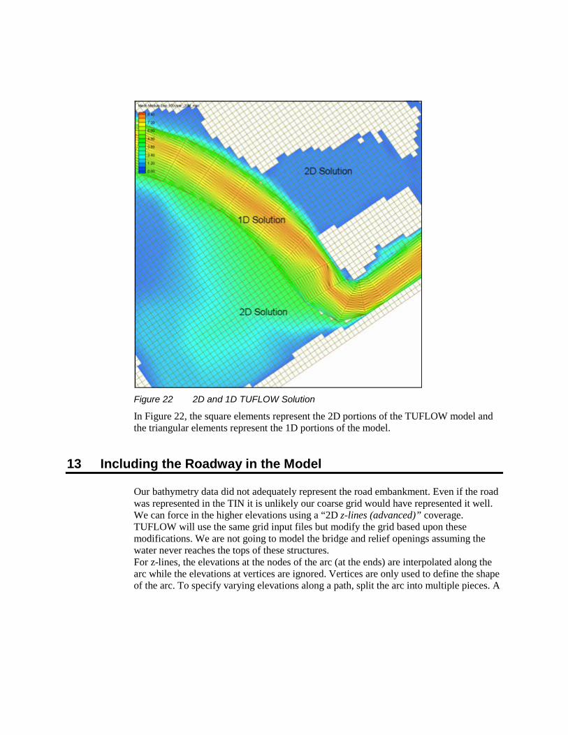
Figure 22 2D and 1D TUFLOW Solution

In Figure 22, the square elements represent the 2D portions of the TUFLOW model and the triangular elements represent the 1D portions of the model.

13 Including the Roadway in the Model Our bathymetry data did not adequately represent the road embankment. Even if the road was represented in the TIN it is unlikely our coarse grid would have represented it well. We can force in the higher elevations using a “2D z-lines (advanced)” coverage. TUFLOW will use the same grid input files but modify the grid based upon these modifications. We are not going to model the bridge and relief openings assuming the water never reaches the tops of these structures. For z-lines, the elevations at the nodes of the arc (at the ends) are interpolated along the arc while the elevations at vertices are ignored. Vertices are only used to define the shape of the arc. To specify varying elevations along a path, split the arc into multiple pieces. A

z-polygon (2D Z-Lines/polygons coverage) can be used to raise/lower whole regions of cells. The elevation used for a polygon can be set by double clicking on the polygon using the select polygon tool. To define the roadway arc:

1. Create a TUFLOW “2D Z Lines (advanced)” coverage named roadway.

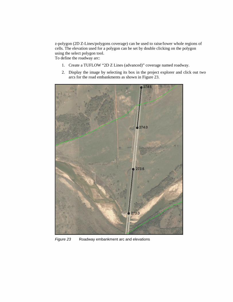
2. Display the image by selecting its box in the project explorer and click out two arcs for the road embankments as shown in Figure 23.

Figure 23 Roadway embankment arc and elevations

3. Change the elevation of each node to the appropriate value as shown in Figure 23.

4. Using the select arc tool, select both newly created arcs, right click and choose “attributes.”

5. Toggle on Override Z values.

6. Change the thickness to width and change the thickness to 10.0 m. This will change all elevations within 5 meters on either side of the z line.

7. Change the option to max. This will make it so it will only change the elevations of cells if the elevation from the z line is higher than the original elevation.

14 New Geometry Component and Simulation Rather than change the existing simulation, we will create a new simulation that includes the roadway. This is a powerful tool which allows multiple configurations to share some of the input files and prevents overwriting earlier solutions. Since the roadway coverage needs to be added to a geometry component, we will also need a new geometry component. To create this component:

1. Right click on the geometry component 20m and select Duplicate.

2. Rename the new component 20m_road.

3. Drag the roadway coverage into the component.

Similarly, we will need to create a new simulation which uses this geometry component. To create and setup the simulation:

1. Right click on the simulation 100year_20m and select Duplicate.

2. Rename the new simulation 100year_20m_road.

3. Right click on the grid component link in the simulation labeled 20m and select delete. This deletes the link to the grid component not the component itself.

4. Drag the geometry component 20m_road into the simulation.

The new simulation will have the same model control and 1D control parameters used previously.

15 Run the New Simulation Repeating the steps above, save the project, export the TUFLOW files, launch TUFLOW, and visualize the results.

16 Conclusion

The simulation message files may contain negative depths warnings which indicate potential instabilities. These can be reduced by increasing the resolution of the grid and decreasing the time step as required. Complete steps for this will not be given, but it should be straight-forward following the steps outlined above. A grid with 10 m cells gives solutions without negative depth warnings. This concludes the TUFLOW 1D/2D tutorial. You may continue to experiment with the SMS interface or you may quit the program.