SNAKE RIVER FALL CHINOOK SALMON LIFE HISTORY INVESTIGATIONS

ANNUAL REPORT 2007

Prepared by:

Kenneth F. Tiffan U.S. Geological Survey

Columbia River Research Laboratory 5501A Cook-Underwood Rd. Cook, Washington 98605

William P. Connor U.S. Fish and Wildlife Service Idaho Fishery Resource Office

P.O. Box 18 Ahsahka, ID 83520

Geoffrey A. McMichael Pacific Northwest National Laboratory

P.O. Box 999 Richland, Washington 99352

Rebecca A. Buchanan

Columbia Basin Research School of Aquatic and Fisheries Sciences

University of Washington 1325 Fourth Avenue, Suite 1820

Seattle, Washington 98101

Prepared for:

U.S. Department of Energy Bonneville Power Administration

Environment, Fish and Wildlife Department P.O. Box 3621

Portland, OR 97208-3621

Project Number 200203200

http://www.efw.bpa.gov/searchpublications/

August 2009

Table of Contents Table of Contents............................................................................................................................ ii Executive Summary ....................................................................................................................... iii Acknowledgements..........................................................................................................................v Chapter One:

Migration delay and survival of juvenile fall Chinook salmon in the vicinity of the confluence of the Snake and Clearwater rivers....................................................................1

Chapter Two:

Hydroacoustic assessment of the abundance of overwintering juvenile fall Chinook salmon in Lower Granite Reservoir, 2007-2008................................................................53

Appendix A:

Assessment of the effect of delayed migration on estimates of the joint probability of migration and survival of juvenile fall Chinook salmon to Lower Granite Dam ..............73

Appendix B:

Fall Chinook salmon SAR estimation and bias correction ................................................76

ii

Executive Summary

In 2007, we used radio and acoustic telemetry to evaluate the migratory behavior,

survival, mortality, and delay of subyearling fall Chinook salmon in the Clearwater River and Lower Granite Reservoir. Monthly releases of radio-tagged fish (~95/month) were made from May through October and releases of 122-149/month acoustic-tagged fish per month were made from August through October. We compared the size at release of our tagged fish to that which could have been obtained at the same time from in-river, beach seine collections made by the Nez Perce Tribe. Had we relied on in-river collections to obtain our fish, we would have obtained very few in June from the free-flowing river but by late July and August over 90% of collected fish in the transition zone were large enough for tagging. Detection probabilities of radio-tagged subyearlings were generally high ranging from 0.60 (SE=0.22) to 1.0 (SE=0) in the different study reaches and months. Lower detection probabilities were observed in the confluence and upper reservoir reaches where fewer fish were detected. Detection probabilities of acoustic-tagged subyearlings were also high and ranged from 0.86 (SE=0.09) to 1.0 (SE=0) in the confluence and upper reservoir reaches during August through October. Estimates of the joint probability of migration and survival generally declined in a downstream direction for fish released from June through August. Estimates were lowest in the transition zone (the lower 7 km of the Clearwater River) for the June release and lowest in the confluence area for July and August releases. The joint probability of migration and survival in these reaches was higher for the September and October releases, and were similar to those of fish released in May. Both fish weight and length at tagging were significantly correlated with the joint probability of migrating and surviving for both radio-tagged and acoustic-tagged fish. For both tag types, fish that were heavier at tagging had a higher probability of successfully passing through the confluence (P=0.0050 for radio-tagged fish; P=0.0038 for acoustic-tagged fish). Radio-tagged fish with greater weight at tagging also had a higher probability of migrating and surviving through both the lower free-flowing reach (P=0.0497) and the transition zone (P=0.0007). Downstream movement rates of radio-tagged subyearlings were highest in free-flowing reaches in every month and decreased considerably with impoundment. Movement rates were slowest in the transition zone for the June and August release groups, and in the confluence reach for the July release group. For acoustic-tagged subyearlings, the slowest movement rates through the confluence and upper reservoir reaches were observed for the September release group. Radio-tagged fish released in August showed the greatest delay in the transition zone, while acoustic-tagged fish released in September showed the greatest delay in the transition zone and confluence reaches. Across the monthly release groups from July through September, the probability of delaying in the transition zone and surviving there declined throughout the study.

iii

All monthly release groups of radio-tagged subyearlings showed evidence of mortality within the transition zone, with final estimates (across the full 45-d detection period) ranging from 0.12 (SE not available) for the May release group to 0.58 (SE = 0.06) for the June release group. The May and September release groups tended to have lower mortality in the transition zone than the June, July, and August release groups. Live fish were primarily detected away from shore in the channel, whereas all dead fish were located along shorelines with most being located in the vicinity of the Memorial Bridge and immediately upstream. During the May detection period, before the implementation of summer flow augmentation, temperatures in the Clearwater River and Snake River arms of Lower Granite Reservoir and the downstream boundary of the confluence ranged from 8 to 17ºC. During the June–August detection periods, however, temperatures in the Clearwater River arm ranged from 10–16ºC down to 7 m and the Snake River arm was above 20ºC down to a depth of 9 m. Incomplete mixing between the two water sources resulted in significant vertical temperature variation at the downstream boundary of the confluence during a large portion of the June–August detection periods. This variation diminished during the September and October detection periods when temperatures once again fell to 17ºC and lower and eventually became uniformly distributed throughout the water column in the confluence. In future years, we will collect run-of-river fish from the lower Clearwater for our tagging efforts to better represent the natural population. In addition, we will concentrate our efforts during July and August in the transition zone and confluence reach to better understand the delay that occurs there during this time. Sample sizes of release groups will be increased as well to obtain more precision for our estimates. During the winter of 2007-2008 we used monthly mobile hydroacoustic surveys from November to March to estimate the number of juvenile Chinook salmon in Lower Granite Reservoir. Concurrent mid-water trawling was used to verify acoustic targets, calculate condition factors, and to compare abundance estimates obtained using hydroacoustics and trawling. Our data indicated that holdover fall Chinook salmon were most abundant and in the best condition in November and December. Thereafter, abundances and relative condition factors decreased. Mean abundance of holdover fall Chinook salmon estimated from hydroacoustic surveys (range 1.15 to 2.19 fish/105 m3) was generally a magnitude less than that estimated from mid-water trawls (range 4.92 to 19.04 fish/105 m3). Our highest monthly population estimate was in December 2007 (11,697; 90 % CI = 7,573 to 15,821) and our lowest monthly population estimate was in January 2008 (6,180; 90% CI = 4,923 to 7,437). In 2008-2009, we will change our hydroacoustic frequency from 420 kHz to 200 kHz to reduce the amount of noise in our data files. We will also use a large lampara seine 228.6 m (750 ft) to attempt to capture more fish and sample the entire water column.

iv

Acknowledgements

We thank our colleagues at the Fish Passage Center, Idaho Fish and Game, NOAA Fisheries, Nez Perce Tribe, Oregon Department of Fish and Wildlife, Pacific Northwest National Laboratory, Pacific States Marine Fisheries Commission, U.S. Army Corps of Engineers, U.S. Fish and Wildlife Service, U.S. Geological Survey, University of Washington, and Washington Department of Fish and Wildlife. We also thank Dale J. Lentz of the U.S. Army Corps of Engineers, Walla Walla District for help in obtaining reservoir storage capacity curves for Lower Granite Reservoir. Finally, we thank Patrick A. Nealson of Hydroacoustic Technology, Inc. for technical and logistical support. Funding for this project was provided by the Bonneville Power Administration and administered by Debbie Docherty. The use of trade names in this report does not imply endorsement by the U.S. Government.

v

CHAPTER ONE

Migration Delay and Survival of Juvenile Fall Chinook Salmon in the Vicinity of the Confluence of the Snake and Clearwater Rivers

Kenneth F. Tiffan U.S. Geological Survey

Columbia River Research Laboratory 5501A Cook-Underwood Rd. Cook, Washington 98605

William P. Connor U.S. Fish and Wildlife Service Idaho Fishery Resource Office

P.O. Box 18 Ahsahka, ID 83520

Geoffrey A. McMichael Marshall C. Richmond

Brian J. Bellgraph William A. Perkins

P. Scott Titzler Ian D. Welch

Jessica A. Carter Katherine A. Deters

Pacific Northwest National Laboratory P.O. Box 999

Richland, Washington 99352

John R. Skalski Rebecca A. Buchanan

Columbia Basin Research School of Aquatic and Fisheries Sciences

University of Washington 1325 Fourth Avenue, Suite 1820

Seattle, Washington 98101

Introduction

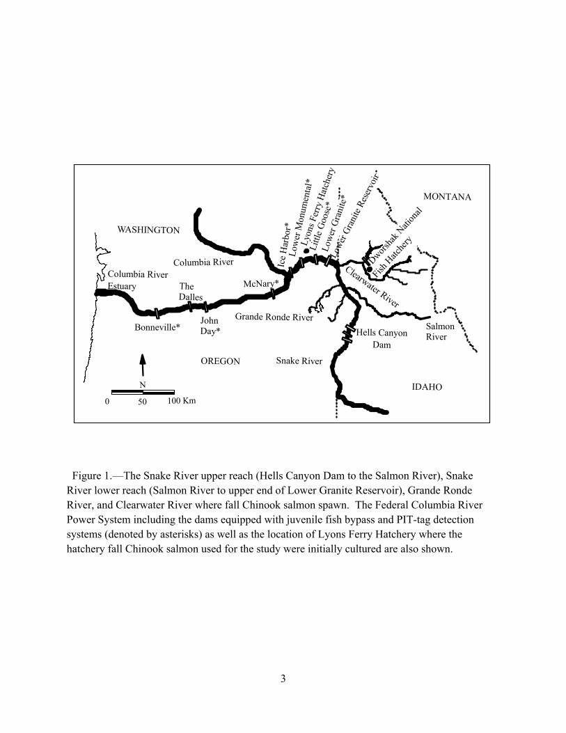
The Snake River upper reach, Snake River lower reach, Grande Ronde River, and Clearwater River are recognized as the four major spawning areas of Snake River Basin natural fall Chinook salmon Oncorhynchus tshawytscha upstream of Lower Granite Reservoir (Figure 1; ICTRT 2007). Though treated as one population, temperature during incubation and early rearing fosters life history diversity among the juveniles produced in these major spawning areas (Connor et al. 2002, 2003). Young fall Chinook salmon in the Snake River upper reach emerge and begin seaward movement earliest in the year followed by fish from the Snake River lower reach, Grande Ronde River, and Clearwater River. Of the four spawning areas, young fall Chinook salmon from the Clearwater River have the most diverse life history. Some of the juveniles meet the seasonal requirements to become actively migrating subyearling smolts and enter the ocean in their first summer of life. Others move downstream gradually, increase their downstream movement rate in the fall, pass Bonneville Dam, and then winter in freshwater or the Columbia River Estuary (Figure 1). A portion of the Clearwater River juveniles begin seaward migration as subyearlings, but eventually lose their disposition to actively migrate and winter in reservoirs formed by the Federal Columbia River Power System. The fish that winter in reservoirs grow to fork lengths above 170 mm and enter the ocean as yearlings. They are referred to as reservoir-type juveniles (Connor et al. 2005).

Understanding the juvenile life history diversity of Clearwater River fall Chinook salmon

juveniles is critical to the recovery of the Snake River Basin fall Chinook salmon population. In 2007, Arnsberg et al. (2009; hereafter Arnsberg et al.) collected data that exemplified the life history diversity of young fall Chinook salmon in the Clearwater River. During June through the first week of August, Arnsberg et al. seined subyearlings rearing along the shorelines of the free-flowing Clearwater River (Figure 2). All subyearlings 60-mm fork length and longer (N = 943) were implanted with passive integrated transponders (PIT tags; Prentice et al. 1990a) and released back to the river. Subyearlings that were large enough to tag were captured from June through the first week of August at a mean fork length of 68 ± 8 mm. A total of 11 of the PIT-tagged fish were eventually recaptured in the free-flowing reaches. The mean residence time (i.e., the number of days that elapsed between initial tagging and recapture) was 6 ± 4 d. This suggests that after growing to 60 mm the fish spent about one week in the free flowing reaches before moving downstream. After moving downstream, the subyearlings traverse a 6-km long reach where the river transitions from a free-flowing to an impounded state. We refer to this area as the “transition zone” that includes both riverine and impounded habitat (Figure 2). The impounded portion makes up the Clearwater River arm of Lower Granite Reservoir. Arnsberg et al. sampled the transition zone from the last week of July to the end of August 2007. In contrast to the free-flowing river, the seine was set at starting points well offshore. A total of 743 subyearlings were captured in the transition zone at an average fork length of 103 ± 12 mm. Of these, 4 had been initially tagged and released from 26 to 40 d earlier in the free-flowing reaches upstream. Three of the subyearlings were recaptured 29 d after they were initially captured and tagged in the transition zone. These findings confirmed that some subyearlings dispersed from

2

Snake River

Columbia River

McNary*

John Day*

The Dalles

Bonneville*

0 50 100 Km

N

Clearwater River

Low

er G

rani

te*

Low

er M

onum

enta

l*

Ice

Har

bor*

OREGON

WASHINGTON

IDAHO

MONTANA

Lyo

ns F

erry

Hat

cher

y

Litt

le G

oose

*Salmon River

Low

er G

rani

te R

eser

voir

Dwor

shak

Nati

onal

Fish H

atche

ry

Grande Ronde River

Hells Canyon Dam

Columbia RiverEstuary

Figure 1.—The Snake River upper reach (Hells Canyon Dam to the Salmon River), Snake River lower reach (Salmon River to upper end of Lower Granite Reservoir), Grande Ronde River, and Clearwater River where fall Chinook salmon spawn. The Federal Columbia River Power System including the dams equipped with juvenile fish bypass and PIT-tag detection systems (denoted by asterisks) as well as the location of Lyons Ferry Hatchery where the hatchery fall Chinook salmon used for the study were initially cultured are also shown.

3

Kayler's Landing rkm 0

Dworshak National Fish Hatchery

rkm 106

Clearwater River

Lower Granite Reservoir

Lower Granite Dam

Upper free-flowing reach

Lower free-flowing reach

Transition zone

Confluence

Upper reservoir

Snake River

rkm 95

rkm 88

rkm 18

rkm 46

rkms 52 and 53

rkm 59

rkm 70

rkm 107rkm 107

rkm 109rkm 114

*

*

*

*

Figure 2.—The study area in 2007 including the reaches of the Clearwater River and Lower Granite Reservoirs where radio (circles) and acoustic (squares) tag detection equipment was stationed, thermographs were located (*), Dworshak National Fish Hatchery where hatchery fall Chinook subyearlings were reared and tagged, and Kayler’s landing where the tagged fish were released. Arnsberg et al. (2009) sampled the upper free-flowing reach, lower free-flowing reach, and the transition zone in 2007.

4

the free-flowing reaches and then spent up to one month or more in the transition zone where they continued to grow.

The downstream passage histories of the subyearlings tagged in both the free-flowing

reaches and transition zone of the Clearwater River by Arnsberg et al. can be described by using PIT-tag detection data. Of the eight hydropower dams juvenile salmon must pass to reach the sea (Figure 1), seven are equipped with juvenile fish bypass systems that contain juvenile PIT-tag detection systems (Prentice et al. 1990b). A PIT-tagged fish can be detected only if it passes via the juvenile fish bypass system of a dam when water is being routed through the system (six to nine months of the year depending on the dam). A PIT-tagged fish that passes a dam via the powerhouse or over the spillways cannot be detected. Detection data can sometimes be used to calculate unbiased estimates of juvenile survival within portions of the hydropower system. This is not the case for Clearwater River subyearlings (Connor et al. 2007). Detection rates are a coarse but useful measure of survival provided that spill levels at the dams do not vary between the time periods being compared. To calculate detection rates, a query is written in the web portal of the PIT-tag Information System (PTAGIS 2006) to determine where and when fish were last detected. The resulting data can then be parsed and sorted to include one “unique last” detection per fish as described hereafter. If a fish was detected at Lower Granite Dam on 8/1/2007 and McNary Dam on 4/15/2008, the unique last detection record for the fish would be the detection at McNary Dam. These data can be used to calculate a detection rate by totaling the unique last detections made across particular “migration years” (e.g., 2007 and 2008) and dividing by the number of fish tagged during an associated “release year” (e.g., 2007). The detection rates for subyearlings tagged in the free-flowing reaches and the transition zone in 2007 by Arnsberg et al. were 9 and 4%, respectively. These differences in detection rates might indicate a possible difference in survival between fish tagged from late June through early August in riverine habitat and fish tagged from late July through the end of August in the transition zone.

The age composition of detected fish can also be calculated from the unique last detection

data. To determine the percentage of detected fish last detected as subyearlings, the total number of unique last detections made in 2007 is divided by the total number of the unique detections made in 2007 and 2008 (and vice versa for yearlings detected in 2008). For the free-flowing reaches of the Clearwater River, 48% of the detected fish tagged by Arnsberg et al. were last detected in 2007 as subyearlings and 52% were last detected as yearlings in 2008. For the transition zone of the Clearwater River, there was a 50/50 split between detections of subyearlings and yearlings.

Another way to analyze PIT-tag data is to query PTAGIS for a set of non-unique last

detections. In this case, the data set includes multiple detections for a fish if it was detected at more than one dam. These data can be used to determine the temporal nature of downstream passage in the Federal Columbia River Power system. Fish tagged in the free-flowing reaches of

5

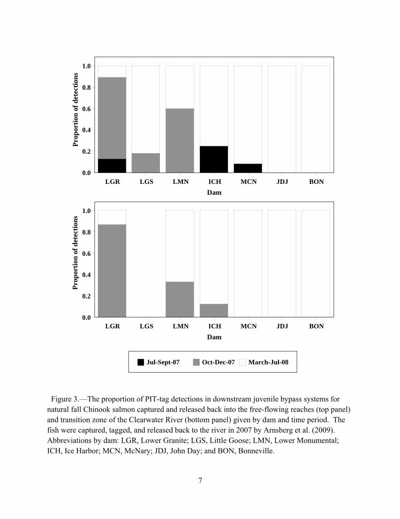
the Clearwater River by Arnsberg et al. were detected at Lower Granite Dam primarily as subyearlings from October to December, but as the fish moved downstream yearling detections became predominant and only yearlings were detected at John Day and Bonneville dams (Figure 3; top panel). Fish tagged in the transition zone of the Clearwater River were detected at Lower Granite Dam primarily as subyearlings from October to December, but as the fish moved downstream yearling detections became predominant and only yearlings were detected at McNary, John Day and Bonneville dams (Figure 3; bottom panel). Three points must be considered when interpreting these data. The first point is that spill was ongoing at all the dams in July and August 2007, thus some PIT-tagged subyearlings passed these dams undetected via the spillways. The second point involves run-at-large fish (i.e., not PIT-tagged). Run-at-large fish that enter the juvenile fish bypass of a dam are not typically routed back to the river. They are routed to raceways, put into barges or trucks, and transported for release downstream of Bonneville Dam. Though summer spill greatly reduced the portion of the run-at-large fish that were transported in 2007, those that were transported had more of an opportunity to enter the sea as subyearlings than inriver migrants because transportation reduced the distance they had to swim to reach the sea. Third, spill was implemented in spring 2008, thus more yearlings passed the dams than the detection data indicate. With these caveats in mind, Figure 3 clearly shows that a substantial number of inriver migrants from the Clearwater River exhibited migration delay in 2007, wintered within the reservoirs of the Federal Columbia River Power System, and entered the sea as yearlings in 2008.

We began a study in 2007 to further understand migration delay and survival of juvenile

fall Chinook salmon. Our original study design included collecting data on fall Chinook salmon from both the Snake and Clearwater Rivers as they passed downstream from riverine habitat to the tailrace of Ice Harbor Dam. This design exceeded the level of available funding, thus we downsized our study and focused on Clearwater River fall Chinook salmon in the vicinity of the confluence of the Snake and Clearwater rivers (hereafter the confluence). Our objectives were to (1) describe the extent and duration of migration delay in the vicinity of the confluence, (2) evaluate the survival of the subyearlings during migration that delay in the vicinity of the confluence, and (3) determine the seasonal biological and environmental factors that affect both migration delay and survival in the vicinity of the confluence. To help develop the study design, we collected pilot data in 2007. In this report, we (1) use the 2007 data collected by Arnsberg et al. to evaluate the potential for collecting and tagging subyearlings in the Clearwater River, (2) examine the 2007 pilot data for seasonal changes in migration and survival, (3) use the 2007 pilot data to calculate the joint probability of migration delay and survival and the probability of mortality, and (4) use the 2007 pilot data to determine how the study might identify the biological and environmental factors for migration delay and survival.

6

LGR LGS LMN ICH MCN JDJ BON

Dam

0.0

0.2

0.4

0.6

0.8

1.0

Pro

por

tion

of

det

ecti

ons

March-Jul-08Oct-Dec-07Jul-Sept-07

Dam

LGR LGS LMN ICH MCN JDJ BON0.0

0.2

0.4

0.6

0.8

1.0

Pro

por

tion

of

det

ecti

ons

Figure 3.—The proportion of PIT-tag detections in downstream juvenile bypass systems for natural fall Chinook salmon captured and released back into the free-flowing reaches (top panel) and transition zone of the Clearwater River (bottom panel) given by dam and time period. The fish were captured, tagged, and released back to the river in 2007 by Arnsberg et al. (2009). Abbreviations by dam: LGR, Lower Granite; LGS, Little Goose; LMN, Lower Monumental; ICH, Ice Harbor; MCN, McNary; JDJ, John Day; and BON, Bonneville.

7

Methods

Data Collection

Study area.—Kayler’s Landing was the upstream boundary of our study area in 2007 (rkm 0; Figure 2) and was used to reference distances throughout our study area. The upper portion of Little Goose Reservoir (the reservoir between Lower Granite and Little Goose Dam; Figure 1) was the lower boundary and it was located 114 km downstream from Kayler’s Landing (rkm 114; Figure 2). We divided the study area into reaches based on a combination of the location of tag detection equipment (described later) and habitat characteristics. The fish traversed these reaches in the following order: (1) the upper free-flowing reach, (2) lower free-flowing reach, (3) the transition zone, (4) the confluence, and (5) the upper reservoir (Figure 2).

Fish source and culture.—In 2007, we were not certain if efforts to collect fish in the transition zone would be successful. Therefore, we chose to obtain pilot data by studying hatchery subyearlings. Acquisition of Lyons Ferry Hatchery (Figure 2) fall Chinook salmon subyearlings for our 2007 releases of tagged fish was coordinated under U.S. v. Oregon. In late April, we randomly selected 60 of the subyearlings from the raceway containing the 2,000 fish for our study and examined them for Renibacterium salmoninarum antigen by enzyme-linked immunosorbent assay (ELISA). In addition, gill/kidney/spleen tissue was examined for viruses associated with infectious pancreatic necrosis, infectious hematopoietic necrosis, and viral hemorrhagic septicemia. The ELISA results were low (optical density less than 0.09), and viral tests were negative.

On 10 May, we transported 2,000 subyearlings averaging 80-mm fork length from Lyons Ferry Hatchery to Dworshak National Fish Hatchery using a truck equipped with a 530-L tank. Fish density in the tank was 0.02 kg/L. Temperature in the tank was 12°C, and oxygen was kept near 100% saturation during the 3-h trip. Upon arrival at Dworshak National Fish Hatchery, we reduced the temperature in the tank from 12ºC to 10.0ºC by adding hatchery water over a 1-h period. The subyearlings were then transferred to a 2-m3 circular tank containing 16,014 L of 10ºC hatchery water supplied at 60 L/min. Starting fish density was 0.006 kg/L. The tank was treated with 2.3 kg of coarse water-softening salt (NaCl) immediately after fish transfer, after cleaning, and after weekly formalin treatments (4.2–4.7 ml/L for 1 h). Formalin treatments were necessary to curtail outbreaks of fungus. There were no bacterial or viral epizootics during rearing. We fed the fish a saturation diet (4% of total body weight) starting with No. 1.2 BioDiet growth formula and ending with No. 1.5 BioDiet growth formula. The water volume in the tank was increased to 1,926 L as the fish grew to a maximum density of 0.013 kg/L.

We withheld feed 48 h prior to each monthly tagging event. Twenty-four hours prior to each event, we collected 150 fish from the rearing tank and transferred them evenly into two

8

121-L holding containers constantly supplied with 10.0–12.0ºC hatchery water. Fish density in these containers ranged from 0.005 to 0.022 kg/L.

Tagging and release.—We made monthly releases of the hatchery subyearlings from

May through October (Table 1). One to two days per month, we surgically implanted subyearlings with coded radio tags (Lotek Wireless, Inc., Newmarket, Ontario) and PIT tags following the methods of Adams et al. (1998). The tags we used (model NTC-M-1) measured 12 mm long, 5 mm wide, weighed 0.37 g in air, and had a life expectancy of 45 d. Antenna length was 16 cm. For all tagged fish, the ratio of tag weight to fish weight did not exceed 5%. Immediately after surgery, the fish were placed into 270-L holding containers constantly supplied with 10.0–12.0ºC hatchery water. Fish density in these containers ranged from 0.003 to 0.014 kg/L. From 16 to 24 h after surgery, we trucked the hatchery subyearlings to Kayler’s Landing on the Clearwater River (Figure 1). During each 20-min trip to Kayler’s Landing, oxygen in the tank was kept near 100% saturation. The hatchery subyearlings were acclimated to ambient river temperature (range, 8.3ºC in October to 14.4ºC in June) by gradually draining the tank using a gasoline-powered water pump to gradually replace the raceway water in the tank with river water at a maximum rate of 2ºC warming per hour. Only one fish died post-tagging in 2007. The total number of fish released per month ranged from 91 to 97. Mean fork length at release ranged from 90.2 to 145.5 mm and mean weight ranged from 8.2 to 33.0 g.

We also made releases of hatchery subyearlings from August through October, but these

fish were double tagged with a PIT tag and a Juvenile Salmon Acoustic Telemetry System (JSATS) transmitter (hereafter acoustic tag; Table 1). Two surgeons performed surgeries each day. Fish were anesthetized with 80 mg/L of tricaine methanesulfonate until stage 4 anesthesia was reached (i.e., fish were unable to maintain an upright position in the water column). Fork length (mm) and weight (g) of each fish were measured after they were anesthetized. Fish were then placed on a surgery platform (i.e., foam pad) for tag implantation. In August and September, fish were implanted with 60-d transmitters manufactured by Sonic Concepts (Model E101; mean weight = 0.59 g, SD = 0.01, N = 100) or Advanced Telemetry Systems (mean weight = 0.61 g, SD = 0.01, N = 100). In October, fish were implanted with 120-d transmitters manufactured by Sonic Concepts (mean weight = 0.83 g, SD = 0.01, N = 30). All transmitters had a 10-s pulse repetition interval (PRI). PolyAqua was applied to the foam pad to help maintain the fish’s slime coat and reduce scale loss. Maintenance anesthetic (40 mg MS-222/L of water) was gravity-fed to fish during surgery (about 2 to 3 min) by a small tube inserted in the mouth. Anesthetic-free water was also available to the surgeon and could be adjusted to maintain proper sedation. An 8-mm incision was made parallel and about 2 mm proximal to the ventral midline. The tags were inserted into the peritoneal cavity, and the incision was closed with two simple, interrupted sutures using 5-0 Monocryl (monofilament manufactured by Ethicon). Immediately after surgery, tagged fish were allowed to recover for 24 h and then released at Kayler’s Landing as described for radio-tagged fish. Post-tagging mortalities were

9

Table 1.—Tagging data for six groups of radio-tagged and three groups of acoustic-tagged hatchery fall Chinook salmon released into the Clearwater River at rkm 56 in 2007. The 17 September acoustic tagging is split due to the use of transmitters from two different manufacturers on that date. Tag manufacturers are coded as LT = Lotek Wireless, SC = Sonic Concepts, ATS = Advanced Telemetry Systems.

Tag date

Release date

N

Mean FL (mm±SD)

Mean weight (g±SD)

Tag life (days)

Tag manufacturer

Radio Tags 22-23 May 23-24 May 97 90.2±3.1 8.2±0.8 45 LT 19-20 Jun 20-21 Jun 95 92.9±4.0 8.8±1.2 45 LT 17-18 Jul 18-19 Jul 91 95.4±4.3 9.3±1.4 45 LT 15-16 Aug 16-17 Aug 95 121.7±10.1 20.2±5.5 45 LT 18-19 Sep 19-20 Sep 93 136.1±11.1 28.4±7.4 45 LT 17-18 Oct 18-19 Oct 95 145.5±10.6 33.0±7.4 45 LT

Acoustic Tags 17 Aug 18 Aug 142 126.7±11.2 18.1±5.4 60 SC 17 Sep 18 Sep 90 133.7±13.5 28.5±9.5 60 ATS 17 Sep 18 Sep 59 135.9±9.8 29.3±6.4 60 SC 16 Oct 17 Oct 122 149.4±7.4 37.3±5.7 120 SC

less than 2% during all three releases (August, n = 2; September, n = 0; October, n = 0). The releases were made at temperatures ranging from 9.9–12.0ºC over the three release dates.

Detecting tagged fish.—We monitored the movement of radio-tagged fish by using arrays

of antennas and receivers located at various fixed detection sites between Kayler’s Landing and the tailrace of Lower Granite Dam (Figure 1). Four- or nine-element Yagi antennas were used at each site in conjunction with a Lotek SRX 400 receiver (Lotek Wireless, Inc., Newmarket, Ontario). One or two receivers were deployed at each fixed detection site to maximize coverage of the river channel. Receivers were powered by 12-V batteries and solar panels. Receivers recorded the tag code, signal strength, and the time and date of each signal emitted by the tag (i.e., every 20 s) while in the vicinity of the receivers. Data from receivers were downloaded twice a week.

Radio-tag data were processed to remove erroneous data records and produce a final

dataset for analyses. Detection records were first arranged in sequential order by time and date. Records that did not fit a logical sequence in space or time, those with low signal strength, or represented by a single observation at a detection site were considered false positives and removed from further consideration. Acceptable detection data were typified by high signal

10

strengths, multiple records at a detection site, and progression of detections as fish moved downstream.

Mobile tracking crews monitored radio-tagged subyearlings three times a week from May

to October in the transition zone. Mobile tracking was conducted from a boat equipped with a 3-element Yagi antenna, and a Lotek SRX400 receiver. A total of 127 parallel transects were established perpendicular to the shoreline in 50-m intervals from the railroad bridge across the Clearwater River (rkm 52) to the Potlatch Mill (~rkm 46). This ensured complete coverage of the transition zone during tracking. On each day of tracking, a GPS was used to navigate each transect beginning with the downstream-most transect. The locations of detected radio-tagged fish were recorded on maps and with a GPS at the point of the strongest signal strength. The gain on the tracking receiver was manually adjusted to obtain the most precise location of tracked fish. An attempt was made to mobile track acoustically tagged fish; however, problems with mobile tracking equipment precluded the use of these data in fate analyses.

Acoustic telemetry receiving nodes (Model N201, Sonic Concepts, Inc., Bothell, WA)

were deployed at locations shown in Figure 2. Nodes had a maximum detection range of about 300 m and were arranged in arrays to detect fish across the entire river width. Two nodes were required to detect fish across the river channel at most arrays; however, the width of the river at the Lower Granite Dam forebay array (approximately 900 m) required the use of three nodes. Each node consisted of a receiver powered by lithium batteries and one 15-s beacon transmitter; node rigging included three buoys, an acoustic release mechanism (Model 111, InterOcean Systems, Inc., San Diego, CA), anchor line, and anchor. The beacon transmitted a signal once every 15 s and was used to confirm that the receiver was working properly. The line between the node and acoustic release was made of 12.5-mm braided nylon rope with braided 9.5-mm SeaDog nylon thimbles at each end; three yellow buoys (Baolong BL-6, 16.5 x 12.4 cm, 1.45 kg buoyancy each) were threaded onto the line. The acoustic release was linked to a 27-kg steel anchor with a 12.5-mm braided nylon rope. The anchor end of the rope was secured using a 4.8-cm shackle, and the opposing end contained a 10-cm-diameter galvanized steel ring held by the acoustic release mechanism.

Acoustic nodes were serviced (i.e., data downloaded and batteries replaced) once each

month between deployment on 10 August 2007 and recovery on 11 and 12 February 2008. To recover nodes, the boat was positioned near the node waypoint and an acoustic transducer (Model 1100E, InterOcean Systems Inc. San Diego, CA) was used to activate the acoustic release and detach the node assembly from the anchor. Once at the surface, the node and release were collected and brought into the boat. An external LED light on the node housing was activated to verify that data were recording at the time of recovery. Battery packs were replaced and data were downloaded from an onboard Compact Flash (CF) card (SanDisk Extreme III 1.0 GB) to a laptop computer. Data were cursorily examined to determine if the node functioned properly during deployment. Nodes with potential problems were removed from service and

11

replaced with a spare. To activate the node for redeployment, we connected the node to a laptop computer and monitored the real-time data collected by the receiver. First, the node clock was synchronized with a GPS clock. Functionality of the node hydrophone was then tested by listening for the beacon transmitter. Three detections of the beacon transmitter by the receiver were required before the node was re-deployed. After passing the three-detection test, a blank CF card was inserted into the node and the node was resealed for deployment. All mechanical components were checked for wear and replaced if necessary, and the node was returned to the water at approximately the same location as recovery. Time and water depth (meters) were recorded at deployment. Location coordinates of the node were recorded using Fugawi Marine ENC GPS software (Northport Systems Inc., Toronto, ON).

Data collected by the acoustic nodes were recorded as text files on CF cards. These text

files were transferred to a laptop computer when the acoustic receivers were serviced during the season or when recovered at the end of the season. Physical data were written to file every 15 s. Physical data recorded included date, time, barometric pressure, water temperature, tilt, and battery voltage. Detections of transmitters were recorded in real time as they were received. They were written to media with TagID (individual code of transmitter), time stamp, receive signal strength indicator, and RxThreshold (a calculated measure of noise). Data files from all acoustic receivers were coded with the acoustic receiver location and stored in a database developed specifically for storing and processing acoustic telemetry data (TagViz). To filter out false positives (detections of TagIDs that did not meet criteria to be considered a valid detection), a post-processing program was used. This program compared each detection to a list of tags that were released (only tags that were released were kept), then compared the detection date to the release date (only tags detected after they were released were kept). A minimum of four detections in 120 s was required, and the time spacing between these detections had to match the PRI of the tag, or be a multiple of the PRI for the detections to be kept in the valid detection file.

Hydrodynamic data.—These data were collected in Lower Granite Reservoir in 2007 and

2008 to supplement data collected in the reservoir in 2002 (Cook et al. 2003) and 2005 (Cook et al. 2006). Self-contained temperature loggers and a portable conductivity-temperature-depth (CTD) probe were used to measure water temperature (Figure 2). A majority of loggers were Onset HOBO® Pro v2 Water Temperature Data Loggers, which have an accuracy of 0.2ºC between −20ºC and 70ºC. One Onset HOBO 76-Meter Depth Data Logger with an accuracy of 0.37ºC at 20ºC and an effective range from −20ºC to 50ºC was also used. SeaBird SBE39 temperature and pressure loggers were also used and had an accuracy of 0.002ºC between −5ºC and 35ºC. Seabird SBE39 loggers (20 m or 100 m maximum depth range) were calibrated to be accurate within 0.1 m. The accuracy of all temperature loggers was confirmed before deployment on 28 June 2007 and after deployment on 13 February 2008 using a constant temperature water bath; any not meeting quality specifications were calibrated. A Hydrolab-Hach MiniSonde 4a portable CTD probe was used to collect temperature profiles and had an accuracy of 0.10ºC in water temperatures from −5ºC to 50ºC. The CTD probe also measured

12

pressure (100-m water depth range with an accuracy of 0.3 m) and specific conductance (±1% of reading and ±0.001 mS/cm). Calibration of the specific conductance sensor was verified each day in the field using standard conductivity solutions. Water temperature data were also obtained from a continuously operated logger string located just outside the Lower Granite forebay boat restricted zone. Cross-sectional CTD profiles were collected along each acoustic Doppler current profiler (ADCP) transect (described later) to ensure CTD probe temperature profiles coincided with logger data. Cross-sectional CTD profile transects between (mixing zone) and upstream (pre-mixing zone) of logger sites provided additional vertical and lateral CTD profile data. Conductivity-temperature-depth profile and water measurement locations were collected using a Trimble Pathfinder Pro XRS differential global positioning system (DGPS) receiver. The integrated DGPS beacon receiver and antenna provided DGPS corrections to calculate accuracy to within 0.5 m. Data Analyses

Potential for collecting fish inriver.—We compared the dates Arnsberg et al. PIT tagged natural subyearlings to the release dates of the radio-tagged and acoustic-tagged hatchery subyearlings to determine how the releases overlapped. On a monthly basis we compared the mean fork length of the fish PIT tagged by Arnsberg et al. to the mean fork length of the radio-tagged and acoustic-tagged fish. We calculated the percentage of the natural subyearlings that exceeded the 7.1 g minimum weight for radio-tag implantation. Together, these analyses were used to determine: (1) when and where we could have radio and acoustic tagged natural subyearlings, (2) how many fish we could have tagged, and (3) what portion of the natural population the radio-tagged and acoustic-tagged fish would have represented.

Tag life.—We measured radio tag life (d) in the hatchery subyearlings by keeping a

subsample (n = 4-6) of each monthly tag group in a circular tank at Dworshak National Fish Hatchery and monitoring the tags 24 h/d with a receiver. A total of 25 radio-tagged fish were monitored until tags expired. We measured the life of the 120-d acoustic tags (N = 30) by surgically implanting acoustic tags into live juvenile fall Chinook salmon, holding them in a circular tank at the Pacific Northwest National Laboratory’s Aquatic Research Laboratory, and monitoring the tags 24 h/d with an acoustic receiver. Data on the life of the 60-d acoustic tags (N = 100 for each manufacturer) were collected similarly to 120-d acoustic transmitters.

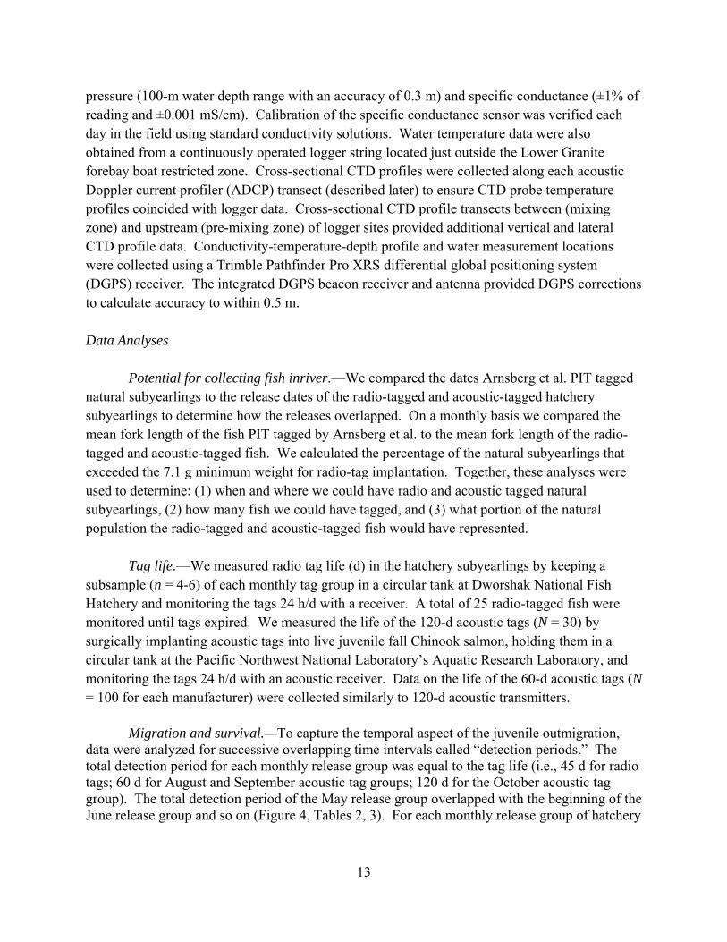
Migration and survival.—To capture the temporal aspect of the juvenile outmigration,

data were analyzed for successive overlapping time intervals called “detection periods.” The total detection period for each monthly release group was equal to the tag life (i.e., 45 d for radio tags; 60 d for August and September acoustic tag groups; 120 d for the October acoustic tag group). The total detection period of the May release group overlapped with the beginning of the June release group and so on (Figure 4, Tables 2, 3). For each monthly release group of hatchery

13

Figure 4.—Time line of release dates and total detection periods for each of the monthly release groups of radio-tagged (top panel) and acoustic-tagged (bottom panel) hatchery fall Chinook salmon in the 2007. Sample sizes are printed above each release.

14

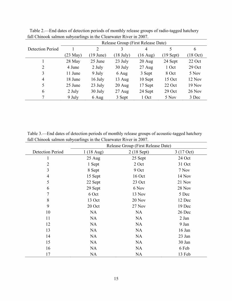
Table 2.—End dates of detection periods of monthly release groups of radio-tagged hatchery fall Chinook salmon subyearlings in the Clearwater River in 2007.

Release Group (First Release Date) Detection Period 1

(23 May) 2

(19 June) 3

(18 July) 4

(16 Aug) 5

(19 Sept) 6

(18 Oct) 1 28 May 25 June 23 July 20 Aug 24 Sept 22 Oct 2 4 June 2 July 30 July 27 Aug 1 Oct 29 Oct 3 11 June 9 July 6 Aug 3 Sept 8 Oct 5 Nov 4 18 June 16 July 13 Aug 10 Sept 15 Oct 12 Nov 5 25 June 23 July 20 Aug 17 Sept 22 Oct 19 Nov 6 2 July 30 July 27 Aug 24 Sept 29 Oct 26 Nov 7 9 July 6 Aug 3 Sept 1 Oct 5 Nov 3 Dec

Table 3.—End dates of detection periods of monthly release groups of acoustic-tagged hatchery fall Chinook salmon subyearlings in the Clearwater River in 2007. Release Group (First Release Date)

Detection Period 1 (18 Aug) 2 (18 Sept) 3 (17 Oct) 1 25 Aug 25 Sept 24 Oct 2 1 Sept 2 Oct 31 Oct 3 8 Sept 9 Oct 7 Nov 4 15 Sept 16 Oct 14 Nov 5 22 Sept 23 Oct 21 Nov 6 29 Sept 6 Nov 28 Nov 7 6 Oct 13 Nov 5 Dec 8 13 Oct 20 Nov 12 Dec 9 20 Oct 27 Nov 19 Dec 10 NA NA 26 Dec 11 NA NA 2 Jan 12 NA NA 9 Jan 13 NA NA 16 Jan 14 NA NA 23 Jan 15 NA NA 30 Jan 16 NA NA 6 Feb 17 NA NA 13 Feb

15

subyearlings, we used the single-release recapture model (Cormack 1964; Skalski et al. 1998) to estimate the probability of detection at each fixed-site radio station or acoustic array, as well as the joint probability of migration and survival through each reach and within the detection period. We refer to the latter of these probabilities as being “joint” because we could not determine whether a fish that was not detected by a fixed-site radio station or acoustic array exiting a reach (1) delayed its migration in the reach through the end of the detection period or (2) died within the reach. We estimated this joint probability of migration and survival through the upper free-flowing reach, the lower free-flowing reach, and the transition zone for the radio-tagged hatchery subyearlings. We estimated the joint probability of migration and survival through the confluence and the upper reservoir for both radio-tagged and acoustic-tagged fish.

Migration delay was categorized in two ways. The first approach identified slow-moving

fish as temporarily delayed within a reach, while the second approach categorized delayed fish as those that remained and survived in a reach through the end of the detection period. The former approach (“movement rate approach”) focuses on fish that eventually passed through and out of a reach, but spent a longer period of time in the reach than most migrants. The latter approach (“probabilistic approach”) focuses on fish that entered but did not exit a reach. This approach distinguishes between mortality in the reach and long-term residence and survival. Thus, the two approaches to describing migration delay focus on two separate groups of fish: fish that eventually left the reach (movement rate approach), and fish that remained in the reach at the end of each detection period (probabilistic approach).

The movement rate approach is based on travel time observations through the reaches,

and so requires only detections at the fixed-site radio stations or acoustic arrays. This approach to measuring migration delay was thus applicable to both radio-tagged and acoustic-tagged subyearlings. The probabilistic approach is based on the exact pattern of detections at all fixed-site receivers, as well as detections from mobile tracking. The available mobile tracking data thus limited the probabilistic approach we used for radio-tagged fish in the transition zone.

The movement rate analysis through a given reach was restricted to tagged subyearlings

that were detected both entering and exiting the reach. For fish with this detection history, the downstream movement rate (km/d) through the reach was calculated as reach length divided by residence time. Residence time (or “travel time”) was calculated for individual fish as the total number of days between reach entry and reach exit. We compared the downstream movement rates and residence times among monthly release groups and reaches to identify seasonal and spatial trends. To evaluate migration delay among fish known to have left the reach, we determined the downstream movement rate that was exceeded 95% of the time (i.e., the 5th percentile of the movement rate distribution). Fish with lower movement rates through a given reach were categorized as “delayed” in that reach. Radio-tag and acoustic-tag data were analyzed separately. The movement rate distribution used to characterize migration delay for radio-tagged fish consisted of movement rates through the transition zone, confluence, and upper

16

reservoir from all releases of radio-tagged fish. For acoustic-tagged fish, the movement rate distribution used to characterize migration delay consisted of movement rates through the confluence and upper reservoir from all releases of acoustic-tagged fish. We calculated the percentage of all fish with movement rate observations in each release group that exhibited migration delay, and compared the percentages across monthly release groups and reaches to identify seasonal and spatial trends. Finally, we used reach entry and exit detection data to determine how many fish that exhibited migration delay were present in each reach on any given day.

Joint probability of migration delay and survival and the probability of mortality.—We

used the probabilistic approach of characterizing migration delay for radio-tagged fish in the transition zone. For this analysis, mobile tracking in the transition zone provided data that were used to distinguish between mortality and migration delay within a reach among those fish that did not exit the reach within the detection period. More precisely, the mobile tracking data were used to determine what proportion of those fish that did not exit the reach remained alive within the reach until the end of the detection period. A fish was assumed to be dead if it was detected at the same location in three or more weekly mobile tracking surveys. A fish was assumed to be alive if it was detected one or more times at unique locations through time.

We analyzed the mobile tracking data with the Manly-Parr model to estimate the number

of fish from each release group that were alive in the transition zone at the end of each detection period (Seber 1982: 233-236). These estimates were combined with estimates of both the joint probability of migration and survival through the transition zone and the number of fish that entered the transition zone to estimate the probability of remaining alive in the reach until the end of the time period, i.e., the joint probability of migration delay and survival in the transition zone. We then estimated the probability of mortality in the transition zone within each detection period, based on the relation that the joint probability of migration and survival, the joint probability of migration delay and survival, and the probability of mortality sum to 1.

This analysis was performed repeatedly for successively longer detection periods. Each

detection period began at the time of initial release at Kayler’s Landing (Figure 1). Successive detection periods ended a week apart (Table 2). Estimated probabilities for each detection period had inference to the fish that entered the transition zone at any time before the end of the detection period. For example, if the joint probability of migration delay and survival was 0.7 for the first detection period (i.e., for the first week after release), then approximately 70% of the fish that entered the transition zone within the first week after release were still alive and residing in the transition zone at the end of that week. If the joint probability of migration delay and survival was 0.1 for the third detection period (ending three weeks after release), approximately 10% of the fish that entered the transition zone within the first three weeks after release were still alive and residing in the transition zone at the end of the third week from release.

17

We plotted the estimates of the joint probability of migration delay and survival within the transition zone for each release group and for each of the successively longer detection periods, for a total of 45 days from release. We then compared results across release groups to examine seasonal trends. We used the same approach for estimates of the probability of mortality within the transition zone. Biological factors for migration and survival.—We explored the potential effects of fish length and weight at tagging on the joint probability of migration and survival through various reaches. For radio-tagged subyearlings, the joint probability of migration and survival was analyzed through the upper free-flowing reach, lower free-flowing reach, transition zone, and confluence. For several radio-tagged releases, there were insufficient radio-tag detections downstream of the confluence to estimate the joint probability of migration and survival through the upper reservoir; thus, analysis of biological factors for radio-tagged subyearlings is limited to the first four reaches. For acoustic-tagged subyearlings, the joint probability of migration and survival was analyzed through the combined free-flowing reaches and transition zone, and separately through the confluence and upper reservoir. A proportional hazards model was used with individual-based covariates to analyze the joint probability of migration and survival using Program SURPH (Smith et al., 1994).

We regressed travel time from release through the confluence onto fish length and fish weight. Travel time was analyzed separately for radio-tagged and acoustic-tagged subyearlings. Travel times were analyzed on the log scale. Environmental factors for migration delay and mortality.—In this report, we evaluated temperature only within the confluence to determine how the study might identify the environmental factors for migration delay and survival. In the future, we plan to model velocity and temperature from the upstream boundaries of the transition zone of the Clearwater River and the upstream boundary of the Snake River arm of Lower Granite Reservoir to the downstream boundary of the upper reservoir reach. In 2007, we described the thermal environment for the period 24 May 2007 to 16 February 2008. We used the 10-min temperature measurements from individual loggers within a string to calculate the hourly minimum, maximum, and depth-averaged temperature over the vertical profile. Depth-weighted average temperature was computed by assigning each logger a portion of the water column. The vertical temperature profile data were analyzed to quantify and classify the strength of a thermal layer, if present. We defined “thermal layer” as the portion of the water column in which the temperature was above the depth-weighted average temperature of the entire profile. The “thermal layer depth” was the depth at which the water column temperature was equal to the depth-weighted average. The temperature in the thermal layer ranged from the profile depth-weighted average to the maximum. This range was termed the “thermal layer temperature delta.” These values were computed at hourly intervals for each logger string. Hourly thermal layer statistics were used to assign a thermal layer classification as follows:

18

(1) if the temperature range over the entire profile was less than 1ºC, that hour was

automatically assigned a layer class of 0 (and its layer depth was plotted as 0 m);

(2) a layer class of 0 was also assigned if the thermal layer temperature delta was less than 1ºC (a layer depth was still computed and plotted);

(3) a layer class of 1 was assigned if the thermal layer temperature delta was more than 1ºC, regardless of the layer depth;

(4) a layer class of 2 was assigned only if the thermal layer temperature delta was more than 2ºC and the layer depth was greater than 5 m.

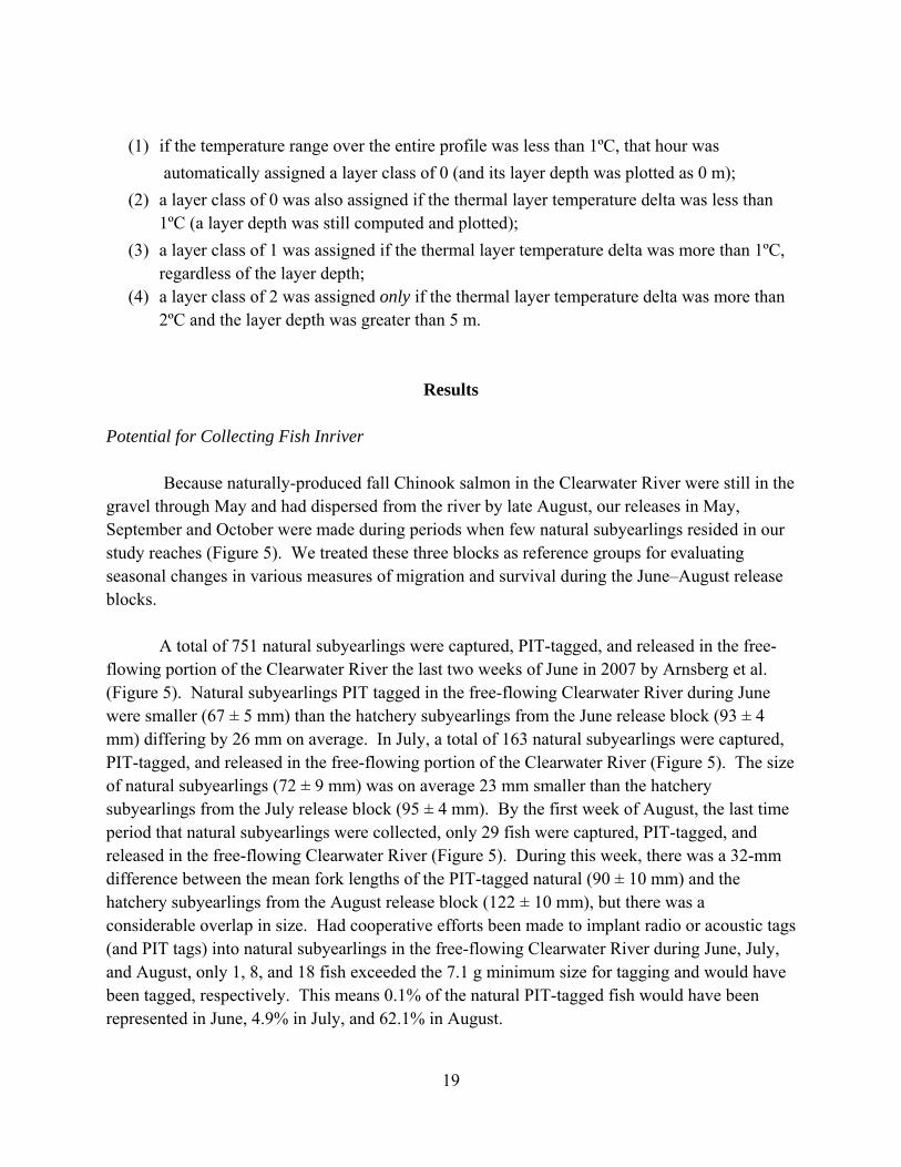
Results Potential for Collecting Fish Inriver Because naturally-produced fall Chinook salmon in the Clearwater River were still in the gravel through May and had dispersed from the river by late August, our releases in May, September and October were made during periods when few natural subyearlings resided in our study reaches (Figure 5). We treated these three blocks as reference groups for evaluating seasonal changes in various measures of migration and survival during the June–August release blocks.

A total of 751 natural subyearlings were captured, PIT-tagged, and released in the free-flowing portion of the Clearwater River the last two weeks of June in 2007 by Arnsberg et al. (Figure 5). Natural subyearlings PIT tagged in the free-flowing Clearwater River during June were smaller (67 ± 5 mm) than the hatchery subyearlings from the June release block (93 ± 4 mm) differing by 26 mm on average. In July, a total of 163 natural subyearlings were captured, PIT-tagged, and released in the free-flowing portion of the Clearwater River (Figure 5). The size of natural subyearlings (72 ± 9 mm) was on average 23 mm smaller than the hatchery subyearlings from the July release block (95 ± 4 mm). By the first week of August, the last time period that natural subyearlings were collected, only 29 fish were captured, PIT-tagged, and released in the free-flowing Clearwater River (Figure 5). During this week, there was a 32-mm difference between the mean fork lengths of the PIT-tagged natural (90 ± 10 mm) and the hatchery subyearlings from the August release block (122 ± 10 mm), but there was a considerable overlap in size. Had cooperative efforts been made to implant radio or acoustic tags (and PIT tags) into natural subyearlings in the free-flowing Clearwater River during June, July, and August, only 1, 8, and 18 fish exceeded the 7.1 g minimum size for tagging and would have been tagged, respectively. This means 0.1% of the natural PIT-tagged fish would have been represented in June, 4.9% in July, and 62.1% in August.

19

05/18 06/01 06/15 06/29 07/13 07/27 08/10 08/24 09/07 09/21 10/05 10/19

Date

0

100

200

300

400

500

600N

um

ber

tag

ged

an

d r

elea

sed

Natural free-flowingNatural transition zoneRadio-taggedAcoustic-tagged

Figure 5.—The number of natural fall Chinook salmon that were captured, PIT-tagged, and released into the Clearwater River upper and lower free-flowing reaches, and transition zone by Arnsberg et al. (2009) and the number of hatchery fall Chinook salmon subyearlings that were radio or acoustic tagged prior to release at Kayler’s Landing along the Clearwater River in 2007. A total of 739 natural subyearlings were captured, PIT-tagged, and released in the transition zone of the Clearwater River from the last week of July through the third week of August (Figure 5). During these 5 weeks, there was only a 5-mm difference between the mean fork lengths of the PIT-tagged natural (104 ± 12 mm) and the hatchery subyearlings from the July release block (109 ± 15 mm). Of the natural subyearlings, 90.9% exceeded the 7.1 g minimum weight for radio-tag implantation. Had cooperative efforts been made to implant radio or acoustic tags into natural subyearlings in the transition zone of the Clearwater River during July and August, the resulting sample size would have been 672 fish and these fish would have represented a large majority (90.9%) of the natural PIT-tagged fish.

20

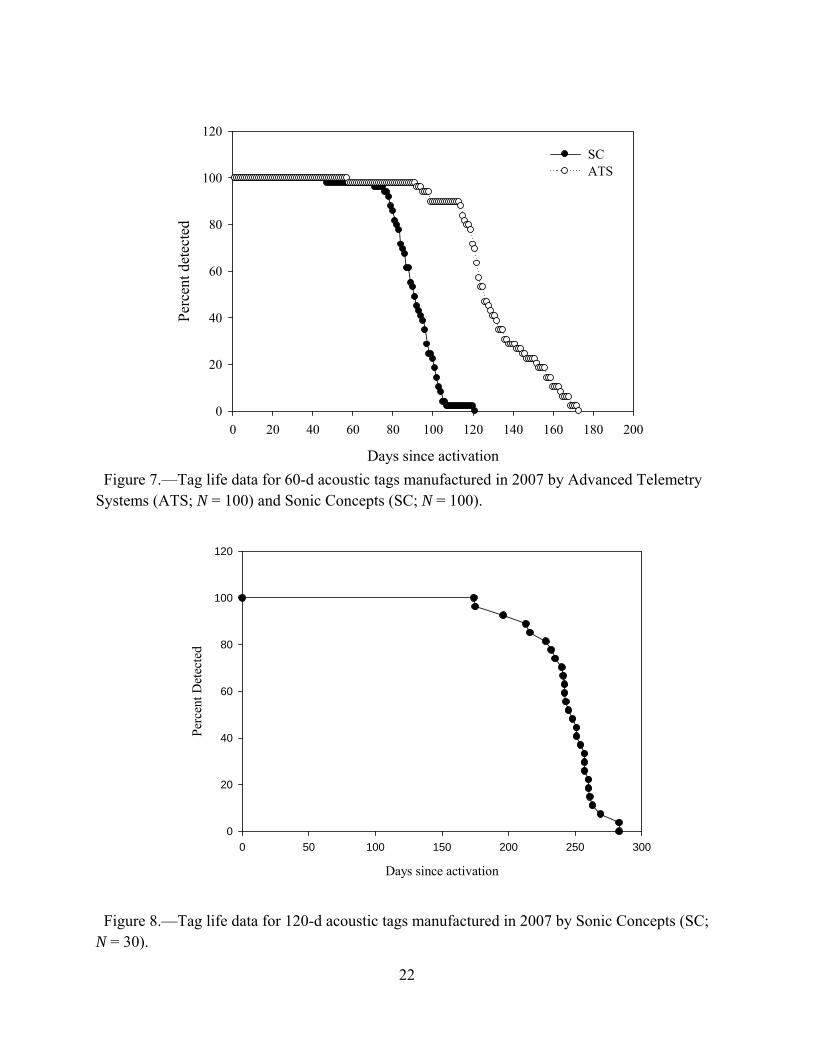
Tag Life Approximately 50% of the 45-d Lotek radio tags failed by day 82. Minimum radio tag

life was 24 d and maximum radio tag life was 102 d (Figure 6). Approximately 50% of the 60-d Sonic Concepts acoustic transmitters failed by day 90 and about 50% of the 60-d Advanced Telemetry Systems acoustic transmitters failed by day 125 (Figure 7). The first 120-d acoustic transmitter died at day 170 and about 50% of the 120-d transmitters had expired batteries by day 246 (Figure 8).

Days since activation

0 20 40 60 80 100 120

Per

cen

t d

etec

ted

0

20

40

60

80

100

120

Figure 6.—Tag life data for 45-d radio tags manufactured in 2007 by Lotek Wireless. (N = 24).

21

Days since activation

0 20 40 60 80 100 120 140 160 180 200

Per

cent

det

ecte

d

0

20

40

60

80

100

120

SCATS

Figure 7.—Tag life data for 60-d acoustic tags manufactured in 2007 by Advanced Telemetry Systems (ATS; N = 100) and Sonic Concepts (SC; N = 100).

Days since activation

0 50 100 150 200 250 300

Per

cent

Det

ecte

d

0

20

40

60

80

100

120

Figure 8.—Tag life data for 120-d acoustic tags manufactured in 2007 by Sonic Concepts (SC; N = 30).

22

Total detections and Detection Probabilities

Detections on the fixed-site receivers that defined the study reaches are given for each monthly release group, along with the conditional probability of detection at each array, for radio-tagged fish (Table 4) and acoustic-tagged fish (Table 5). For the radio-tagged release groups, detection numbers were high for most monthly release groups at the entrance to the lower free-flowing reach. The exception was the September release group, which had only 48 fish detected entering that reach. The number of radio-tagged subyearlings detected entering the transition zone ranged from 31 for the September release group to 90 for the May release group, while the number detected entering the confluence ranged from 24 for both the June and September release groups to 68 for the May release group. The June–September release groups had relatively few fish detected entering the upper reservoir (10–16), compared to the May and October release groups (60 and 52 fish detected, respectively). Detection probabilities for the radio-tagged subyearlings were generally high, ranging from 0.60 (SE=0.22) at the receiver defining the downstream boundary of the upper reservoir for the August release group, to 1.000 (SE=0) for multiple receivers throughout the study area and for all monthly release groups (Table 4). Sparse detection data at receivers downstream of the upper reservoir prevented estimation of the detection probability at the exit of the upper reservoir for the June, July, and September release groups (Table 4).

Detection information is available only for the confluence and upper reservoir reaches for

the acoustic-tagged release groups (Table 5). Detections at the entrance to the confluence ranged from 48 fish from the September release group to 83 fish for the October release group. For the upper reservoir, detections of entering fish ranged from 21 for the August release group to 75 for the October release group (Table 5). Detection probabilities at the downstream boundaries of these two reaches ranged from 0.86 (SE=0.09) for August release group leaving the upper reservoir to 1.00 (SE=0) for the October release group leaving the upper reservoir (Table 5). Seasonal Changes in Migration and Survival

The estimates of the joint probability of migration and survival for the June–August release groups of radio-tagged hatchery subyearlings declined markedly in the transition zone (Figure 9; top panel). The estimate for the June release group was lower through the transition zone than through the confluence, whereas the estimates for the July and August release groups were higher through the transition zone than through the confluence. This pattern suggests that biological and environmental factors affecting the estimates changed between detection periods of the June release group and the July–August release groups. Furthermore, whatever the influential specific factors were, they were not strongly in effect within the transition zone during the detection periods of the May, September, and October release groups, or within the confluence during the detection periods of the May and October release groups (Figure 9, bottom panel; Figure 10). Estimates of the joint probability of migration and survival through the upper

23

Table 4.—Final detections and detection probabilities (SE) for the May–October release groups of radio-tagged hatchery fall Chinook salmon subyearlings in 2007 given by study reach. Notation: n1, the number of subyearlings detected entering; n2, the number of subyearlings

detected exiting; n3, the number of subyearlings detected both entering and exiting; and (and standard error), detection probability for the fixed station located at the downstream end of the reach.

P̂

Month of release (release size)

Reach Detection

information

May (97)

June (95)

July (91)

August

(95)

September

(93)

October

(95) Upper free

flowing

n1 97 95 91 95 93 95 n2 94 79 82 82 48 82 n3 94 79 82 82 48 82 P̂ 1.000

(0) 1.000

(0)0.973

(0.019)0.974

(0.018)0.968

(0.032) 0.973

(0.019) Lower free

flowing

n1 94 79 82 82 48 82 n2 90 59 74 76 31 74 n3 90 59 72 74 30 72 P̂ 0.987

(0.013) 1.000

(0)1.000

(0)1.000

(0)1.000

(0) 1.000

(0)

Transition zone

n1 90 59 74 76 31 74

n2 68 24 45 41 24 67 n3 67 24 45 41 24 67 P̂ 0.851

(0.041) 1.000

(0)1.000

(0)1.000

(0)0.938

(0.061) 0.982

(0.018)

Confluence n1 68 24 45 41 24 67 n2 60 15 10 12 16 52 n3 53 15 10 12 15 51 P̂ 0.781

(0.052) 1.000

(0)0.667

(0.272)0.857

(0.132)1.000

(0) 0.895

(0.050)

Upper reservoir

n1 60 15 10 12 16 52

n2 53 2 2 5 5 34 n3 43 2 2 4 5 31 P̂ 0.814

(0.051) NA NA0.600

(0.219) NA 0.840

(0.073)

24

Table 5.—Final detections and detection probabilities (SE) for the August–October release groups of acoustic-tagged hatchery fall Chinook salmon subyearlings in 2007 given by study reach. Notation: n1, the number of subyearlings detected entering; n2, the number of subyearlings detected exiting; n3, the number of subyearlings detected both entering and exiting; and (and standard error), detection probability for the acoustic node located at the downstream end of the reach.

P̂

Month of release (release size)

Reach Detection

information

August (142)

September

(147)

October

(121) Confluence n1 62 48 83

n2 32 41 75 n3 28 36 70 P̂ 0.950

(0.049)0.966

(0.034)0.962

(0.026)

Upper n1 32 41 75 reservoir n2 18 28 53

n3 18 28 51 P̂ 0.857

(0.094)0.952

(0.047)1.000 (0)

25

Figure 9.— The joint probability of migration and survival (%, with 95% confidence interval) through the five study reaches for radio-tagged (RT) and acoustic-tagged (AT) hatchery fall Chinook salmon subyearlings in 2007, given by monthly release group.

26

Figure 10.— The joint probability of migration and survival (%, with 95% confidence interval) through the transition zone of the Clearwater River (top panel) and confluence of the Snake and Clearwater rivers (bottom panel) for radio-tagged (RT) and acoustic-tagged (AT) hatchery fall Chinook salmon subyearlings in 2007, given by monthly release group.

27

reservoir were available only for the acoustic-tagged release groups and for the August and October release groups of radio-tagged subyearlings. Although point estimates tended to be higher for the upper reservoir than for the confluence for the August release groups, and lower for the upper reservoir than for the confluence for the September and October release groups, the estimates had low precision for the downstream reach, making interpretation difficult (Figure 9). Too few radio-tagged subyearlings released in May through July and in September were detected downstream of the upper reservoir to make it possible to estimate the joint probability of migrating and surviving through that reach for those release groups.

As previously mentioned, downstream movement rate and residence times could be

calculated only for those subyearlings that were detected both entering and exiting a reach (i.e., n3 in Tables 4 and 5). In general, movement rates were measured for more fish for the free-flowing reaches than for the downstream reaches, with the fewest observations for the upper reservoir (Tables 4 and 5). For radio-tagged subyearlings, movement rates were measured for over 90 fish from the May release group for both the upper and lower free-flowing reaches, but for only 2 fish in the upper reservoir for both the June and July release groups. The sparse movement rate data available for the downstream reaches and for the June and July release groups means that movement rate patterns should be interpreted with caution.

For the radio-tagged subyearlings with movement rate observations, median movement

rates per release group ranged from 0.6 km/d for the August release group through the transition zone to 160.1 km/d for the May release group through the upper free-flowing river (Figure 11, top panel). For the radio-tagged release groups, 95% of the individual movement rates calculated for the transition zone, confluence, and upper reservoir exceeded 0.37 km/d; fish with movement rates <0.37 km/d through one of these reaches were classified as “delayed” in that reach. For the acoustic-tagged subyearlings with movement rate observations, median movement rates per release group ranged from 1.7-1.8 km/d in the upper reservoir for both the August and September release groups, to 12.1 km/d in the confluence for the October release group (Figure 11, bottom panel). For the acoustic-tagged release groups, 95% of the individual movement rates calculated for the confluence and the upper reservoir exceeded 0.23 km/d; acoustic-tagged fish with movement rates <0.23 km/d through one of these reaches were classified as “delayed” in that reach.

In general, the movement rate through the free-flowing reaches decreased through the

study season, with the median movement rate through the lower free-flowing reach at 106.1 km/d for the May release group of radio-tagged subyearlings, but only at 33.1 km/d for the October release group (Figure 11, top panel). For each monthly release group of radio-tagged subyearlings, the median movement rate in the transition zone was considerably lower than the median movement rate through the free-flowing reaches. Median movement rates through the

28

Figure 11.—Median downstream movement rate (km/d) in the study reaches for radio-tagged (RT, top panel) and acoustic-tagged (AT, bottom panel) hatchery fall Chinook salmon subyearlings in 2007 given by monthly release group. Numbers above bars indicate the number of fish with movement rate observations for the reach.

29

transition zone range from 0.6 km/d for the August release group to 20.1 km/d for the May release group (Figure 11, top panel). This pattern suggests that any environmental factors that influenced migration delay were present in higher proportion in the transition zone than in the free-flowing reaches. This is supported by the finding that the percentage of radio-tagged fish (with movement rates) that were classified as “delayed” (i.e., movement rate <0.37 km/d) was positive for the transition zone for all release groups except October, with the August release group having the highest proportion of delayed migrants (Figure 12, top panel). The time period with the highest number of radio-tagged subyearlings residing in the transition zone was in late August, for a total of 261.7 fish days from the August release group (Figure 13, top panel).

Movement rates through the confluence were also low for the July, August, and

September radio-tagged release groups, but higher for the May, June, and October radio-tagged release groups (Figure 11, top panel). Likewise, movement rates were higher for the October release group of acoustic-tagged fish than for the earlier release groups (Figure 11, bottom panel). For radio-tagged subyearlings, the median movement rate through the confluence ranged from 2.1 km/d for the August release group, to 34.6 km/d for the May release group (Figure 11, top panel). For acoustic-tagged subyearlings, the median movement rate through the confluence ranged from 2.7 km/d for the September release group to 12.1 km/d for the October release group (Figure 11, bottom panel). Using the radio-tag criterion for delay (i.e., movement rate <0.37 km/d), only the September release group included fish that delayed in the confluence (2 fish, 13.3%; Figure 12, top panel). Using the acoustic-tag criterion for delay (i.e., movement rate <0.23 km/d), all three release groups included delayed fish in the confluence, with 4.6% (1 fish) from the August release group, 11.1% (4 fish) from the September release group, and 1.4% (1 fish) from the October release group showing delay. There was at least one live study fish (acoustic-tagged) present in the confluence through early December before it moved downstream (Figure 14, top panel).

Movement rates through the upper reservoir were generally calculated on fewer fish than

for the upstream reaches. Movement rates were lower through the upper reservoir than through the confluence for the May, June, and October radio-tagged groups and all three acoustic-tagged groups (Figure 11). For radio-tagged subyearlings, median movement rates through the upper reservoir ranged from 2.0 km/d for both the September and October release groups, to 14.4 km/d for the June release group (based on 2 fish). For acoustic-tagged fish, median movement rates through the upper reservoir ranged from approximately 1.7 km/d for both the August and September release groups to 2.4 km/d for the October release group. Only one radio-tagged fish was classified as having delayed in the upper reservoir (i.e., movement rate <0.37 km/d; Figure 12, top panel). This fish, from the October release group, resided in the upper reservoir for 30 days before moving downstream (Figure 13, bottom panel). For acoustic-tagged subyearlings, three fish from the September release group and 2 fish from the October release group were classified as delayed (i.e., movement rate <0.23 km/d; Figure 12, bottom panel). One of the

30

Figure 12.— The percentage of downstream movement rates that were small enough to be classified as “delayed,” for radio-tagged (RT, top panel) and acoustic-tagged (AT, bottom panel) hatchery fall Chinook salmon subyearlings in 2007 given by monthly release group. Numbers above bars indicate the number of fish with movement rate observations for the reach.

31

Figure 13.— The number of radio-tagged hatchery fall Chinook salmon present each day in the transition zone (top panel), confluence (middle panel), and upper reservoir (bottom panel) that were classified as “delayed” based on movement rate through the reach (i.e., movement rate <0.37 km/d) in 2007.

32

Figure 14.— The number of acoustic-tagged hatchery fall Chinook salmon present each day in the confluence (top panel) and upper reservoir (bottom panel) that were classified as “delayed” based on movement rate through the reach (i.e., movement rate <0.23 km/d) in 2007.

33

September fish remained in the upper reservoir through late December (69 days) before moving downstream (Figure 14, bottom panel). Seasonal Changes in the Joint Probability of Migration Delay and Survival and the Probability of Mortality in the Transition Zone

The joint probability of migration delay and survival for radio-tagged hatchery

subyearlings in the transition zone is given by successively longer detection periods (Figure 15, top panel). For each date shown, the reported point estimate is the estimated joint probability of delaying migration in the transition zone and surviving there through the indicated date, conditional on having entered the transition zone at any time before that date (and after release). For example, fish from the August release group that entered the transition zone within the first week after release (i.e., before August 20) had a high probability of delaying migration and surviving there until August 20 (0.69, SE=0.04), indicated by the first point estimate for the August release group in Figure 15 (top panel). Fish released in August that entered the transition zone before August 27 had only a 0.32 (SE=0.02) probability of remaining and surviving in the transition zone through August 27, indicated by the second point estimate for the August release group in Figure 15 (top panel). By the beginning of October, only 1 live fish from the August release group was detected via mobile tracking within the transition zone, and so the estimated probability of remaining and surviving in the transition zone throughout September was very low (0.13, no SE estimate available). Mobile tracking in the transition zone ended in late October, so estimates of the joint probability of migration delay and survival in that reach were unavailable after October 25.

The May release group showed no migration delay of surviving fish in the transition

zone, while all later release groups exhibited some migration delay in that reach (Figure 15, top panel). The August release group exhibited the highest proclivity to delay in the transition zone, with nearly 70% (SE=4.9%) of the fish that entered the transition zone within the first week after release remaining there (and surviving) throughout the week. The September release group also had a high estimated probability of delaying and surviving in the transition zone within the first week after release (0.43, SE=0.11). There was less delay exhibited by the June and July release groups, and those that did delay within the transition zone tended to take longer to travel to that reach than in the August and September releases. For the June release group, the estimated probability of migration delay and survival in the transition zone peaked three weeks after release at 0.11 (SE=0.01), while for the July release group, the estimated probability peaked in the second week after release at 0.23 (SE=0.03). Across the monthly release groups, the probability of remaining in the transition zone and surviving there declined throughout the study period. For the release groups with mobile tracking throughout the full 45-d detection period (i.e., May – August), no more than 1 live fish from each release group was detected via mobile tracking in the transition zone at the end of 45 d. These findings suggest that biological and environmental factors affecting migration delay and survival were not in effect during the May

34

Figure 15.—The joint probability of migration delay and survival (±1.96×SE; top panel) and the probability of mortality (±1.96×SE; bottom panel ) given by end of detection intervals for monthly release groups of radio-tagged hatchery fall Chinook salmon subyearlings in the transition zone of the Clearwater River in 2007. All detection intervals began at the release date.

35

detection period, grew stronger from the June through August detection periods, and began to weaken slightly during the September detection period.

Estimates of the probability of mortality for the radio-tagged hatchery subyearlings in the

transition zone depended on having available estimates of both the joint probability of migration and survival and the joint probability of delay and survival. The estimated probability of mortality in the transition zone is given throughout the study period for each monthly release group (Figure 15, bottom panel). For each date given, the point estimate is the estimated probability of dying in the transition zone before that date, for fish that entered that reach before that date. All monthly release groups showed evidence of mortality within the transition zone, with final estimates (across the full 45-d detection period) ranging from 0.12 (SE not available) for the May release group to 0.58 (SE = 0.06) for the June release group. For the June, July, and October release groups, mortality estimates dropped from the first week to the second week (Figure 15, bottom panel), indicating that fish arriving in the transition zone in the first week tended to experience more mortality there than fish arriving in the second week. The May and September release groups tended to have lower mortality in the transition zone than the June, July, and August release groups. These findings suggest that biological and environmental factors affecting mortality were present during the May detection period, became much stronger during the June detection period, decreased in strength slightly and leveled off during the July and August detection periods, and then grew substantially weaker during the September detection period.

The locations and fates of radio-tagged subyearlings mobile tracked in the transition zone

of the Clearwater River are summarized only for May-September releases. Mobile tracking was not done for the October release because all fish moved rapidly through the transition zone during this time of year. Both live and dead fish were detected during mobile tracking (Figures 16-17). Live fish were primarily detected away from shore in the channel, but some were detected along the shorelines (Figures 16-17). The median times live fish spent in the transition zone ranged from 7 to 19.5 d for fish released from May to September, and individual fish resided from 1 to 78 d (Table 6). Many fish moved up and downstream while in the transition zone. The median upstream distances (>100 m) moved by fish ranged from 160 to 414 m for fish released from June to September with individual fish moving up to 1,788 m upstream (Table 7). We were unable to determine if fish moved downstream past our lowermost detection site on the Clearwater River, entered the Snake River, and then returned to the Clearwater River. Some fish that were originally known to be alive in the transition zone subsequently died. For monthly releases made from May through August, 1, 4, 5, and 10 fish, respectively, were initially classified as being alive, but then subsequently fit our criteria for being dead (Table 6). For fish released in September, 14 of 18 fish tracked were known to be alive, but there was an insufficient amount of subsequent mobile tracking effort to determine if any fish died in the transition zone from that release. All dead fish were located along the shorelines with most being located in the vicinity of the Memorial Bridge and immediately upstream (Figures 16-17).

36

Boatramp

MemorialBridge

RailroadBridge

x

x

x

xx

x

x

ooo

N Release 1(May)

O = live fish, N=13X = dead fish, N=7

Flow

MemorialBridge

RailroadBridge

x xx

x

x

x x o

o

o

N

x

x xx

xo

o

o

o

o

ooo

oo

Release 2(June)

Boatramp

O = live fish, N=13X = dead fish, N=12

Flow

MemorialBridge

RailroadBridge

x xx

x

x

x

o

o

o

N

xxx

oo

o

o oo

oo

o

oRelease 3

(July)Boatramp

5 fish

o

o

o

o

o

o

o

o

oO = live fish, N=23X = dead fish, N=13

Flow

Figure 16.—Locations and fates of radio-tagged subyearling fall Chinook salmon that were mobile tracked in the transition zone of the lower Clearwater River in 2007 during Releases 1-3.

37

Boatramp

MemorialBridge

RailroadBridge

x

xx

x

x

x

oo

o

N Release 4(August)

xx

x

x

3 fish

oooooo

oo

oo

o oooo

o

oo

o

oo

o

ooo

ooooo

o ooooo

o

oo

ooo

ooo

o

o

o

o

oo

o

O = live fish, N=56X = dead fish, N=12

Flow

MemorialBridge

RailroadBridge

o

o

o

N

o

o o

o

o

o

o

oo

Release 5(September)

Boatramp

o

oo

o

o

o

O = live fish, N=18X = dead fish, N=0

Flow

Figure 17.—Locations and fates of radio-tagged subyearling fall Chinook salmon that

were mobile tracked in the transition zone of the lower Clearwater River in 2007 during Releases 4-5.

38

Table 6.—Summary of fate information from radio-tagged subyearling fall Chinook salmon that were mobile tracked in the transition zone in the lower Clearwater River in 2007.

Release

Number

tracked

Number

alive

Number

dead

Number

alive

then

dead

Median

(range)

residence

time of live

fish (d)

Median

number

of weeks

dead fish

detected

Minimum

number of

weeks

dead fish

detected

Maximum

number of

weeks

dead fish

detected

May 9 2 7 1 19.5 (19-20) 10 6 12

June 20 9 11 4 13 (1-61) 12 6 14

July 31 18 13 5 9 (1-78) 10 4 13

Aug 59 46 13 10 13 (1-66) 9 3 10

Sept 18 18a 7 (1-24) aOf these fish, 14 were known to be alive, but mortality could not be determined because the reach was

not tracked for a sufficient number of weeks

Table 7.—Summary of upstream distances moved by radio-tagged subyearling fall Chinook salmon residing in the transition zone of the lower Clearwater River in 2007. Data are for fish that moved at least 100 m.

Release

Number of fish

Median upstream distance moved (m)

Minimum upstream distance moved (m)

Maximum upstream distance moved (m)

June 5 269 135 1,212 July 9 300 150 878

August 31 414 128 1,788 September 5 160 150 731

39

Dead fish were detected in the same locations from 3 to 14 weeks (median = 10 weeks; Table 6). Limited mobile tracking conducted in the free-flowing reaches of the Clearwater River and in the confluence reach showed mortality was occurring there as well.

The joint probability of migration and survival, joint probability of migration delay and

survival, and the probability of mortality calculated for the final detection period of each monthly release group are given in Table 8. Given that the probability of migration delay and survival through the transition zone was low for all monthly release groups with available estimates, we can conclude that the joint probability of migration and survival largely reflected overall survival through the transition zone for the hatchery subyearlings studied. This may or may not have been the case for the confluence and upper reservoir reaches.

Biological Factors for Migration and Survival Both fish weight and length at tagging were significantly correlated with the joint probability of migrating and surviving for both radio-tagged and acoustic-tagged fish. For both tag types, fish that were heavier at tagging had a higher probability of successfully passing through the confluence (P=0.0050 for radio-tagged fish; P=0.0038 for acoustic-tagged fish; Figure 18). Radio-tagged fish with greater weight at tagging also had a higher probability of migrating and surviving through both the lower free-flowing reach (P=0.0497) and the transition zone (P=0.0007; Figure 18). The effect of fish length at tagging was more ambiguous. In general, radio-tagged subyearlings that were longer at tagging had a lower probability of migrating and surviving through each of the free-flowing reaches, the transition zone, and the confluence (P=0.0065; Figure 19). Acoustic-tagged fish that were longer at tagging, however, were more likely to successfully migrate through the combined free-flowing reaches and the transition zone (P=0.0409; Figure 19). In general, the acoustic-tagged subyearlings were larger than the radio-tagged subyearlings, with acoustic-tagged fish averaging 27.6 g and 136.3 mm at tagging, and radio-tagged fish averaging 18.3 g and 113.6 mm at tagging. Additionally, half of the radio-tagged release groups were released before any of the acoustic-tagged release groups. These disparities limit the possibility of a joint analysis of the acoustic-tag and radio-tag data. The conflicting results on the effect of length suggest that the factors influencing migration are complex, and warrant continued study.

40

Table 8.—The joint probability of migration and survival (% ± SE), joint probability of migration delay and survival (% ± SE), and probability of mortality (% ± SE) through the transition zone of the Clearwater River for radio-tagged hatchery fall Chinook salmon subyearlings for the final detection period (45 d) in 2007. In some cases, the SE could not be calculated because of sparse mobile tracking data. Estimates of the joint probability of migration delay and survival and of the probability of mortality were available only for 35 days for the September release group, and for 7 days for the October release group, because mobile tracking was ended in the third week of October.

Release group

Joint probability of migration and survival

Probability of delay

Probability of mortality

Total

May 87.6 ± 3.7 0.0 12.4 100.0 June 40.7 ± 6.4 1.7 ± 0.1 57.6 ± 6.4 100.0 July 60.8 ± 5.7 1.4 ± 0.1 37.8 ± 5.7 100.0

August 54.0 ± 5.7 1.3 ± 0.0 44.7 ± 0.0 100.0 September 84.6 ± 7.6 NA NA NA

October 92.2 ± 3.2 NA NA NA

41

Figure 18.—The fitted probability of migrating and surviving through various study reaches versus weight at tagging for radio-tagged (RT, top panel) and acoustic-tagged (AT, bottom panel) subyearling Chinook salmon in 2007. Only reaches with significant weight effects are shown. The fitted probability was calculated at the average length at tagging: 113.6 mm for radio-tagged fish, and 136.3 mm for acoustic-tagged fish.

42

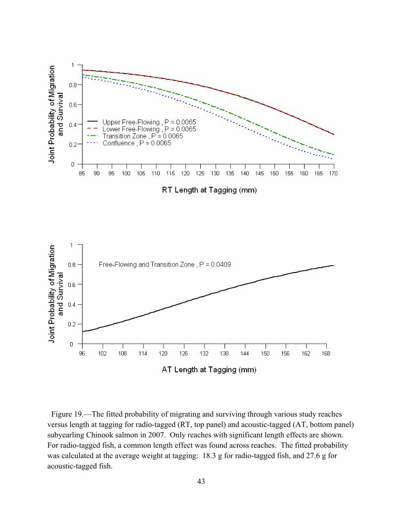
Figure 19.—The fitted probability of migrating and surviving through various study reaches versus length at tagging for radio-tagged (RT, top panel) and acoustic-tagged (AT, bottom panel) subyearling Chinook salmon in 2007. Only reaches with significant length effects are shown. For radio-tagged fish, a common length effect was found across reaches. The fitted probability was calculated at the average weight at tagging: 18.3 g for radio-tagged fish, and 27.6 g for acoustic-tagged fish.

43

Environmental Factors for Migration Delay

Earlier in this report, we showed that the migration delay increased and the joint probability of migration and survival through the confluence decreased after the May detection period. Migration delay decreased and the joint probability of migration and survival increased to levels similar to those observed during the May detection period and during the September and October detection periods. During the May detection period, temperatures in the Clearwater River and Snake River arms of Lower Granite Reservoir and the downstream boundary of the confluence ranged from 8 to 17ºC (Figure 20). During the June–August detection period, however, temperatures in the Clearwater River arm ranged from 10–16ºC down to 7 m and the Snake River arm was above 20ºC down to a depth of 9 m (Figure 20). Incomplete mixing between the two water sources resulted in significant vertical temperature variation at the downstream boundary of the confluence during a large portion of the June–August detection periods (Figure 20). This variation diminished during the September and October detection periods when temperatures once again fell to 17ºC and lower and eventually became uniformly distributed throughout the water column through the confluence (Figure 20).

44

Figure 20.—Vertical temperature profiles for the Clearwater River arm of Lower Granite Reservoir (top panel) and the Snake River arm of Lower Granite Reservoir (middle panel), and the downstream boundary of the confluence (bottom panel) in 2007. The detection periods for the radio-tagged and acoustic-tagged hatchery fall Chinook salmon subyearlings are given in the top and middle panels, respectively.

45

Discussion

As shown by Arnsberg et al., some natural subyearlings disperse from the free-flowing reaches and then spend extended periods of time in the transition zone where they continued to grow. Differences observed in detection rates of the natural subyearlings PIT tagged by Arnsberg et al. might indicate that earlier migrating fish tagged in the free-flowing Clearwater River survive at higher rates than later migrating fish tagged in the transition zone. A substantial number of inriver migrants from the Clearwater River lose their disposition to migrate and winter within the reservoirs of the Federal Columbia River Power System, and enter the sea as yearlings in 2008. Understanding migration delay and survival of Clearwater River fall Chinook salmon destined to become reservoir-type juveniles is critical to the recovery of the Snake River Basin fall Chinook salmon population.

By using the 2007 data collected by Arnsberg et al. we were able to evaluate the potential

for collecting and tagging subyearlings in the Clearwater River. Consistent with other years (e.g., Connor et al. 2002), we found that relatively few natural fall Chinook salmon would be large enough to tag by the end of May (Arnsberg et al. 2007). Had cooperative efforts been made with Arnsberg et al. to implant radio or acoustic tags (and PIT tags) into natural subyearlings in the free-flowing Clearwater River during June and July, the resulting sample size would have been small and the fish tagged would have represented only a fraction of the natural PIT-tagged fish. The natural fish we could have tagged in the free-flowing river during the first week of August would have represented a slight majority (62.1%) of the natural PIT-tagged fish, but the sample size would have only been 18 because the majority of the natural population had already dispersed downstream. Had cooperative efforts been made to implant radio or acoustic tags into natural subyearlings in the transition zone of the Clearwater River during July and August, the resulting sample size would have been 672 fish and these fish would have represented a large majority (90.9%) of the natural PIT-tagged fish.

In the future years of our study, we will cooperate with Arnsberg et al. to increase the number of fish collected in the transition zone. Sampling could begin in late July and be conducted through mid August with a 300 ft lampara seine or by hook and line. All fish less than 7.1 g (the minimum weight for transmitter implantation) could be PIT-tagged by NPT to support the work of Arnsberg et al. We could divide the fish larger than 7.1 g between NPT staff and our staff. NPT staff could PIT-tag their portion. We could transport the remaining portion of fish ≥7.1 g to a location upstream of the transition zone where they could be given 24 h to recover in circular tanks constantly supplied with de-gassed river water. We could then implant radio tags and PIT tags, or acoustic tags and PIT tags, into the fish and then allow them to recover for 24 h in the circular tanks after which they will be released at the site of tagging.

Though the data we collected on hatchery subyearlings in 2007 were not intended for making inferences to the natural population, there were some similarities between the hatchery

46

subyearlings and natural subyearlings in the Clearwater River that should be considered when planning future work. First, we found some evidence for a seasonal change in survival. The May, September, and October release groups had higher joint probabilities of migration and survival throughout all of the study reaches than were observed for the June – August release groups. Additionally, the May and September release groups had lower probabilities of mortality in the transition zone than the June–August release groups. In future years, we should consider including May and October reference groups to contrast with releases of inriver fish made in July and August. The May release group could be seined along the shoreline of the Snake River, tagged, and released into the Clearwater River as described above. The October release group could be captured by using a lampara seine in Lower Granite Reservoir and tagged and released into the Clearwater River as described above. The second similarity between the natural hatchery subyearlings was that both groups exhibited migration delay in the transition zone. In the future, it would be useful to collect velocity and temperature data in the transition zone and the portion of the free-flowing river the fish will have to traverse after release to enter the transition zone. This will provide us with the ability to completely model the habitat available to natural subyearlings in the vicinity of the confluence. It will help us to determine the seasonal biological and environmental factors that affect both migration delay and survival in the vicinity of the confluence. Movement rates of subyearlings through the Clearwater River and Lower Granite Reservoir reaches were generally slower that those reported by Tiffan et al. (2009a) for presumably active migrants in the Snake River. Only the migration rates for subyearlings moving through the free-flowing reaches of the Clearwater River in May were similar to those of subyearlings moving through riverine reaches of the Snake River. The migratory disposition of fish in each study may explain the differences. Tiffan et al. (2009a) collected active migrants from Lower Granite Dam and released them back upstream in the free-flowing Snake River. It is possible that these fish were predisposed to migrate, which was responsible for their faster migration rates. The hatchery fish we used in this study may have been less disposed to migrate rapidly and underscores the need to use run-of-river fish in the future. Nonetheless, the decline in movement rate presumably tracked the decline in water velocities from a free-flowing to impounded environment, which is consistent with the findings of Tiffan et al. (2009a). In 2007, we tagged hatchery subyearlings with either a radio tag or acoustic tag. Radio tags provided us with the ability to mobile track in the transition zone and obtain the fate data needed to calculate the joint probability of migration delay and survival and the probability of mortality. However, the precision on these estimates was low because the release numbers were relatively small and some fish died before reaching the transition zone. Releasing more fish and making the releases close to the transition zone would increase the precision of our results in future years. The longer tag life of the acoustic tags provided the opportunity to collect data over a longer time period because of their longer tag life. However, we were not able to mobile track acoustic-tagged fish through the confluence or upper reservoir because of cost and technological

47

limitations. In addition to increasing the number of acoustic-tagged fish released in the future, we should consider increasing the number of acoustic nodes deployed through the confluence and upper reservoir reach. This would allow us to determine fate as shown by McMichael et al. (2008). Both radio and acoustic telemetry have limitations that should be considered when interpreting our results and conclusions. Although we did not examine specific tag effects during this study, we recognize that tagged fish may have had differential behavior and survival compared to untagged fish. The fish we tagged were necessarily large to accommodate tagging, particularly early in the season. The fish we tagged early in the season only represented the larger fish in the natural population, but as the season progressed and natural fish increased in size, later tagged groups represented a larger portion of the natural population. We also acknowledge that there could have been differences between the hatchery fish we tagged and the natural fish we were trying to represent. Hatchery fish were used to ensure that fish were available for tagging at the right time and size. In 2007, we were not certain enough run-of-river fish could be obtained from the lower Clearwater River using beach seines or hook-and-line sampling. However, collections made in 2008 using a lampara seine indicated that run-of-river fish could be collected in future years.

In 2007, we documented migratory delay in subyearlings in the lower Clearwater River. The reasons for this delay are largely speculative but can be supported from a number of lines of reasoning. First, changes in the hydrodynamic environment as the river transitions from a free-flowing to impounded state may alter fish behavior. Tiffan et al. (2009a) recently showed that subyearlings released in the Snake River traveled rapidly through a free-flowing reach but slowed considerably in the upper end of Lower Granite Reservoir. The authors speculated this was due to reductions in water velocity and turbulence cues in this area. The same conditions likely occur in the transition zone of the lower Clearwater River. Although water velocities were not measured in the Clearwater River in 2007, they do slow considerably in the transition zone. It is possible that fish, which traveled comparatively rapidly through the free-flowing river during all months, slow and hold in the slower-moving water in lower Clearwater River, perhaps to feed, which we have routinely observed. Second, the physiological status of subyearlings in the Clearwater River during the summer may contribute to their migratory delay. In contrast to subyearlings in the Snake River that outmigrate under an increasing photoperiod, the later emergence of Clearwater subyearlings results in their outmigration occurring under a decreasing photoperiod. Increasing photoperiod and temperature have been shown to increase smoltification in salmonids (Wedemeyer et al. 1980; Muir et al. 1994). Thorpe (1981) discusses the influence photoperiod has on specific hormones that may be related to downstream movement. It is possible that the combination of decreasing photoperiod (after June 21) and the large reduction in water temperature that accompanies summer flow augmentation may reduce growth (Arnsberg and Statler 1995), physiological development, and the urge to migrate in subyearlings.

48

We found that some fish that delayed or attempted to pass through the transition zone in

the lower Clearwater River experienced mortality. We believe this mortality was due to predation by piscivorous fish such as north pikeminnow Ptychocheilus oregonensis or smallmouth bass Micropterus dolomieu. Shively et al. (1996) documented significant predation on juvenile spring Chinook salmon by northern pikeminnow in the lower Clearwater River following a hatchery release. All dead fish (or their tags) were located along shorelines with many being located together in specific areas whereas most live fish were located offshore. It is likely that predatory fish hold in lower velocities near shore when not feeding and thereby have a greater chance of passing tags of depredated fish in those locations. We also found dead fish along the shorelines of the confluence reach during limited mobile tracking. In future years we plan to radio tag predatory fish to determine if their distribution overlaps with that of dead fish to confirm predation.

Migratory delay in subyearlings produced in the Clearwater River likely contributes to

some fish adopting a reservoir-type life history. The cool water temperatures provided by summer flow augmentation enable fish to reside in the Clearwater River in which temperatures would be very high if no augmentation was provided. Fish that move into Lower Granite Reservoir can use behavioral thermoregulation to select optimal temperatures from a wide range in temperatures (Tiffan et al. 2009b). This strategy enables subyearlings to maximize growth to attain large sizes that make them less vulnerable to predation. However, this delay comes at the cost of increased mortality until such sizes can be attained. Specific causes of migratory delay in Clearwater River subyearlings remain largely unexplored and remain an area of future research.

49

References Adams, N.S., D.W. Rondorf, S.D. Evans, J.E. Kelly, and R.W. Perry. 1998. Effects of surgically

and gastrically implanted radio transmitters on swimming performance and predator avoidance of juvenile Chinook salmon (Oncorhynchus tshawytscha). Canadian Journal of Fisheries and Aquatic Sciences 55:781-787.

Arnsberg, B. D., and D. P Statler. 1995. Assessing summer and fall Chinook salmon restoration

in the upper Clearwater River and principal tributaries. Nez Perce Tribe Department of Fisheries Resources Management 1994 Annual Report to the Bonneville Power Administration, Project 1983350003, Portland, Oregon.

Arnsberg, B. D., D. S. Kellar, and M. A. Tuell. 2007. Nez Perce Tribal Hatchery monitoring

and evaluation; Fall Chinook salmon (Oncorhynchus tshawytscha) supplementation in the Clearwater River Subbasin. 2005 Annual Report to the Bonneville Power Administration, Project 1983350003, Portland, Oregon.

Arnsberg, B. D., D. S. Kellar, and M. A. Tuell. 2009. Nez Perce Tribal Hatchery monitoring

and evaluation of fall Chinook salmon supplementation in the Clearwater River Subbasin. 2007 Annual Report to the Bonneville Power Administration, Project 1983350003, Portland, Oregon.

Connor, W. P., H. L. Burge, R. Waitt, and T. C. Bjornn. 2002. Juvenile life history of wild fall

Chinook salmon in the Snake and Clearwater rivers. North American Journal of Fisheries Management 22:703-712.

Connor, W. P., C. E. Piston, and A. P. Garcia. 2003. Temperature during incubation as one

factor affecting the distribution of Snake River fall Chinook salmon spawning areas. Transactions of the American Fisheries Society 132:1236-1243.

Connor, W. P., J. G. Sneva, K. F. Tiffan, R. K. Steinhorst, D. Ross. 2005. Two alternative

juvenile life histories for fall Chinook salmon in the Snake River basin. Transactions of the American Fisheries Society 134:291-304.

Connor, W. P. B. D. Arnsberg, S. G. Smith, D. M. Marsh, and W. D. Muir. 2007. Post-release

performance of natural and hatchery subyearling fall Chinook salmon in the Snake and Clearwater rivers. Report of the U. S. Fish and Wildlife Service, Nez Perce Tribe, and National Marine Fisheries Service to the U.S. Army Corps of Engineers, Walla Walla, Washington.

Cook, C. B., B. Dibrani, M. C. Richmond, M. D. Bleich, P. S. Titzler, and T. Fu. 2006.

Hydraulic characteristics of the lower Snake River during periods of juvenile fall

50

Chinook salmon migration. PNNL-15532, Pacific Northwest National Laboratory, Richland, Washington.

Cook, C. B., C. L. Rakowski, M. C. Richmond, S. P. Titzler, A. M. Coleman, and M. D. Bleich.

2003. Numerically simulating the hydrodynamic and water quality environment for migrating salmon in the lower Snake River. PNNL-14297, Pacific Northwest National Laboratory, Richland, Washington.

Cormack, R.M. 1964. Estimates of survival from the sighting of marked animals. Biometrika

51:429-438. ICTRT (Interior Columbia River Basin Technical Recovery Team). 2007. Review draft:

Viability criteria for application to interior Columbia Basin ESUs. Available at www.nwfsc.noaa.gov/trt/trt_documents/ictrt_viability_criteria_reviewdraft_2007_complete.pdf

McMichael, G. A., M. C. Richmond, W. A. Perkins, J. R. Skalski, R. A. Buchanan, J. A.

Vucelick, E. E. Hockersmith, B. R. Beckman, P. N. Westhagen, K. D. Ham, I. D. Welch, B. J. Bellgraph, P. S. Titzler, and B. P. Sandford. 2008. Lower Monumental Reservoir Juvenile Fall Chinook Salmon Behavior Studies, 2007. PNWD, Battelle–Pacific Northwest Division, Richland, Washington.

Muir, W. D., W. S. Zaugg, A. E. Giorgi, and S. McCutcheon. 1994. Accelerating smolt

development and downstream movement in yearling Chinook salmon with advanced photoperiod and increased temperature. Aquaculture 123:387-399.

Prentice, E. F., T. A. Flagg, and C. S. McCutcheon. 1990a. Feasibility of using implantable

passive integrated transponder (PIT) tags in salmonids. American Fisheries Society Symposium 7:317-322.

Prentice, E. F., T. A. Flagg, C. S. McCutcheon, and D. F. Brastow. 1990b. PIT-tag monitoring

systems for hydroelectric dams and fish hatcheries. American Fisheries Society Symposium 7:323-334.

PTAGIS (Columbia Basin PIT Tag Information System). 2008. Pacific States Marine Fisheries

Commission, Portland, Oregon. Available: www.ptagis.org. (June 2008). Seber, G.A.F. 1982. The Estimation of Animal Abundance and Related Parameters. Blackburn

Press, Caldwell, New Jersey. Shively, R. S., Poe, T. P., and S. T. Sauter. 1996. Feeding response by northern squawfish to a

hatchery release of juvenile salmonids in the Clearwater River, Idaho. Transactions of the American Fisheries Society 125:230-236.

51

Skalski, J.R., S.G. Smith, R.N. Iwamoto, J.G. Williams, and A. Hoffmann. 1998. Use of PIT tags to estimates survival of migrating juvenile salmonids in the Snake and Columbia Rivers. Canadian Journal of Fisheries and Aquatic Sciences 55:1484-1493.

Smith, S. G., J. R. Skalski, J. W. Schlechte, A. Hoffman, and V. Cassen. 1994. SURPH.1

manual: Statistical survival analysis of fish and wildlife tagging studies. Center for Quantitative Science, School of Fisheries, University of Washington, Seattle, WA.

Tiffan, K.F., T.J. Kock, C.A. Haskell, W.P. Connor, and R.K. Steinhorst. 2009a. Water

velocity, turbulence, and migration rate of subyearling fall Chinook salmon in the free-flowing and impounded Snake River. Transactions of the American Fisheries Society 138:373-384.

Tiffan, K.F., T.J. Kock, W.P. Connor, R.K. Steinhorst, and D.W. Rondorf. 2009b. Behavioural thermoregulation by subyearling fall (autumn) Chinook salmon Oncorhynchus tshawytscha in a reservoir. Journal of Fish Biology 74:1562-1579.

Thorpe, J. E. 1981. Migration in salmonids, with special reference to juvenile movements in

freshwater. Pages 86-97 in E.L. Brannon and E.O. Salo, editors. Salmon and Trout Migratory Behavior Symposium. University of Washington, Seattle.

Wedemeyer, G. A., R. L. Saunders, and W. C. Clarke. 1980. Environmental factors affecting

smoltification and early marine survival of anadromous salmonids. Marine Fisheries Review 42(6):1-14.

52

CHAPTER TWO

Hydroacoustic Assessment of the Abundance of Overwintering Juvenile Fall Chinook Salmon in Lower Granite Reservoir, 2007-2008

Craig A. Haskell and Kenneth F. Tiffan U.S. Geological Survey

Columbia River Research Laboratory 5501A Cook-Underwood Rd. Cook, Washington 98605

53

Introduction

Fall Chinook salmon in the Snake River Basin were listed under the endangered species act in 1992 (NMFS 1992). At that time it was accepted that Snake River fall Chinook salmon exhibited an ocean-type life history in which fry emerged in the spring, grew rapidly, and migrated seaward during the summer to enter the ocean as subyearlings (Healey 1991). However, studies have shown that Snake River fall Chinook salmon also exhibit a reservoir-type life history whereby juveniles delay seaward migration, spend their first winter in lower Snake River reservoirs or freshwater above the estuary, and then resume their seaward migration in the spring as yearlings (Arnsberg and Statler 1995; Connor et al. 2005).

This alternative life history type of fall Chinook salmon has two primary management

implications. First, lower Snake River fish bypass and collection facilities do not operate from December to March. During this period, juvenile fall Chinook salmon that pass lower Snake River dams (Kock et al. 2007) do so primarily through powerhouse turbines, which is the main route of passage during this time of year. Juvenile salmonids that pass dams via the powerhouse are highly susceptible to mortality from blade strike and exhibit higher mortality than those that pass via the fish bypass system (Muir et al. 2001). Second, because many of these fish pass lower Snake River dams without detection during the winter, they likely bias traditional smolt-to-adult return (SAR) ratios which are used to measure the success of juvenile fish transportation relative to in-river migration. Connor et al. (2005) found that juvenile fall Chinook salmon that emigrate from lower Snake River reservoirs in winter and the following spring have high SARs and make a substantial contribution to the eventual number of return spawners that pass Lower Granite Dam. However, transportation studies incorrectly assume that both in-river and transported fish reach the ocean as subyearlings. Therefore, it has become increasingly important to gain information on the abundance, location, and emigration timing of Snake River fall Chinook salmon that exhibit a reservoir-type life history and overwinter in lower Snake River reservoirs. In 2007 we began an effort to determine the number of juvenile fall Chinook salmon that remain in Lower Granite Reservoir during the winter using active hydroacoustics. Our primary objective was to estimate the population of overwintering juvenile salmon and examine population changes through the winter. Furthermore, we examined spatial differences in the population that occurred within Lower Granite Reservoir to locate potential areas where fish reside.

Methods Study area

Lower Granite dam is located 173 km upstream of the Snake and Columbia River confluence. It is the fourth upstream dam on the lower Snake River and the first dam encountered by outmigrating juvenile salmonids originating in the Snake and Clearwater rivers. Lower Granite Reservoir is impounded by Lower Granite Dam, which is located 51 km downstream of the Snake and Clearwater confluence (Figure 1).

54

McNary

Ice Harbor

L. Monumental

Little Goose

Lower Granite

Dworshak

Hells Canyon Oxbow

BrownleeImnaha River

Grande Rhonde River

Salmon River

Clearwater River

Snake River

Columbia River

Clarkston

McNary

Ice Harbor

L. Monumental

Little Goose

Lower Granite

Dworshak

Hells Canyon Oxbow

BrownleeImnaha River

Grande Rhonde River

Salmon River

Clearwater River

Snake River

Columbia River

Clarkston

McNary

Ice Harbor

L. Monumental

Little Goose

Lower Granite

Dworshak

Hells Canyon Oxbow

BrownleeImnaha River

Grande Rhonde River

Salmon River

Clearwater River

Snake River

Columbia River

ClarkstonClarkston

Figure 1.—Map of the Snake River Basin with major tributaries. Open circles denote dams and the star denotes Lower Granite Dam. Trawling Trawling was conducted in conjunction with active hydroacoustics to identify the size and species composition of fish taxa for comparison with fish targets identified by hydroacoustic sampling. Of particular interest was the number and size range of fish that could potentially be confused with juvenile Chinook salmon in hydroacoustic surveys. We also used trawling as an alternative means of estimating abundance of juvenile Chinook salmon for comparison to that estimated from hydroacoustic sampling. Finally, trawling was used to examine changes in the relative condition of juvenile Chinook salmon in Lower Granite Reservoir during winter.

We trawled from the Lower Granite Dam forebay upstream to rkm (river kilometer) 211 (Figure 2) using a monofilament mid-water trawl. The trawl was 12 m long with a rectangular opening of 4.6 m2. A plastic trash can was attached inside the cod end of the trawl to provide a sanctuary to captured fish. After collection, juvenile Chinook salmon were anesthetized with 66 mg/L MS-222, measured to the nearest millimeter fork length, weighed to the nearest 0.1 g, and then released. All other fishes were identified to the lowest practical taxa, measured to the

55

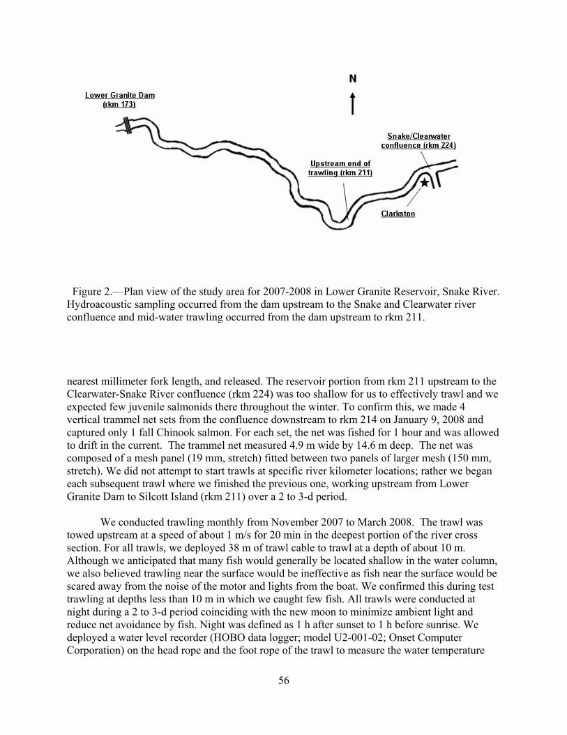
Figure 2.—Plan view of the study area for 2007-2008 in Lower Granite Reservoir, Snake River. Hydroacoustic sampling occurred from the dam upstream to the Snake and Clearwater river confluence and mid-water trawling occurred from the dam upstream to rkm 211. nearest millimeter fork length, and released. The reservoir portion from rkm 211 upstream to the Clearwater-Snake River confluence (rkm 224) was too shallow for us to effectively trawl and we expected few juvenile salmonids there throughout the winter. To confirm this, we made 4 vertical trammel net sets from the confluence downstream to rkm 214 on January 9, 2008 and captured only 1 fall Chinook salmon. For each set, the net was fished for 1 hour and was allowed to drift in the current. The trammel net measured 4.9 m wide by 14.6 m deep. The net was composed of a mesh panel (19 mm, stretch) fitted between two panels of larger mesh (150 mm, stretch). We did not attempt to start trawls at specific river kilometer locations; rather we began each subsequent trawl where we finished the previous one, working upstream from Lower Granite Dam to Silcott Island (rkm 211) over a 2 to 3-d period.

We conducted trawling monthly from November 2007 to March 2008. The trawl was

towed upstream at a speed of about 1 m/s for 20 min in the deepest portion of the river cross section. For all trawls, we deployed 38 m of trawl cable to trawl at a depth of about 10 m. Although we anticipated that many fish would generally be located shallow in the water column, we also believed trawling near the surface would be ineffective as fish near the surface would be scared away from the noise of the motor and lights from the boat. We confirmed this during test trawling at depths less than 10 m in which we caught few fish. All trawls were conducted at night during a 2 to 3-d period coinciding with the new moon to minimize ambient light and reduce net avoidance by fish. Night was defined as 1 h after sunset to 1 h before sunrise. We deployed a water level recorder (HOBO data logger; model U2-001-02; Onset Computer Corporation) on the head rope and the foot rope of the trawl to measure the water temperature

56

and depth of each trawl and to ensure that the trawl was opening properly. We set the recorders to log temperatures and depths in 5-s intervals. Recorders had an advertised depth accuracy of 1.5 cm and temperature accuracy of 0.37ºC. We attached a flow meter (General Oceanics, Inc.) to the trawl to estimate volume of water sampled using flow and the dimensions of the trawl opening. For each trawl, we recorded starting and ending GPS (Global Positioning System) locations, start and end time, and total depth. At the conclusion of trawling, we conducted hydroacoustic sampling. Hydroacoustic sampling We conducted mobile hydroacoustic surveys in Lower Granite Reservoir using a Hydroacoustic Technology Inc. (HTI) model 244 split-beam echo sounder operated at a frequency of 420 kHz. Using the echo sounder, we multiplexed between a 6º ‘side-looking’ transducer and 15º ‘down-looking’ transducer. The down-looking transducer was oriented 90º down from the water surface and the side-looking transducer was oriented 4º down from the water surface. The side-looking transducer was also oriented 90º from the long axis of the boat to ‘look’ straight out from the boat. The transducers were mounted on a tow fin, which was deployed from the starboard side of a 7.3 m boat. The towfin was connected by cable both to a davit from the side of the boat from which depth could be adjusted and to an arm off the starboard side of the bow of the boat from which the towfin could be adjusted fore or aft. We used a GPS (Trimble GeoXT) to navigate pre-set transects and to stream a continuous string of GPS coordinates into the laptop computer during hydroacoustic data collection. Acoustic returns were received and coupled with GPS coordinates using HTI Sounder data collection software (Version 3.56). Boat speed was about 5.6 km/h during surveys. The hydroacoustic system was calibrated using a tungsten calibration sphere prior to data collection. Our primary objective for hydroacoustic sampling was to estimate the number of juvenile Chinook salmon overwintering (hereafter holdovers) in Lower Granite Reservoir. Because our objective was to estimate abundance of fish in the entire reservoir, we sampled the entire reservoir from Lower Granite Dam to the Snake and Clearwater confluence (Rkm 224) near Clarkston, Washington using systematic zigzag transects (Simmonds and MacLennan 2005). The starting and ending points for each transect were 800 m apart. Transect distances varied depending on the sinuosity of the river. The total length of the study area was 50.7 km and we collected data along 63 transects over each 3-d sampling period. We conducted hydroacoustic sampling every month over a three night period immediately following three nights of trawling. All hydroacoustic sampling and trawling was conducted at night. In general, fish in freshwater tend to be more dispersed at night. They move up off the bottom, stay away from the surface, and do not aggregate in schools relative to the daytime. For these reasons, hydroacoustic sampling is often conducted at night as fish are more easily detected at this time. High winds and generally rough conditions negatively affect hydroacoustic system performance and therefore, on occasion, we altered our sampling dates to sample during calm conditions. During our final sampling period in March, we only conducted hydroacoustic sampling from river km 173.0 to 212.6 due to rough weather.

57

Data analysis Trawl catch data were used to examine trends in abundance and relative condition (K) of juvenile Chinook salmon in Lower Granite Reservoir for each sample period. Abundance was calculated from trawls using the volume sampled by the trawl (net opening * flow as calculated from the flow meter) divided by the number of fish collected. Fulton’s condition factor was defined as K = (W/L3)*100,000 (Anderson and Neumann 1996). Fulton’s condition factor is a measure of the relative physiological condition of fish and is useful for comparing fish of similar length of the same species (Pope and Kruse 2007). Raw data collection files were processed using acoustic analysis software (Hydroacoustic Technology, Inc., Echoscape, Version 2.12). Echoscape was used to select acoustic echoes from noise and track them as fish targets. To identify individual fish, we used a combination of an auto-tracking algorithm with user-defined settings and manual editing to separate fish and noise. The auto-tracking algorithm begins by selecting an initial echo which meets specific requirements and then searches in three-dimensional space for the next echo. Groups of echoes are selected as fish targets based on number of pings, echo gap (missing pings), target amplitude, and pulse width at differing decibel levels (power points). We parameterized the auto-tracker to select groups of echoes as fish targets which had a minimum of 4 pings, a maximum ping gap of 5, a maximum target velocity of 5.5 cm/s, a 0.3 m maximum change in distance between echoes, a maximum change in range (target to transducer face) of 0.2 m, and a mean target strength between -70 and -10 dB. According to Love (1971), a fish ranging in length from 170 to 256 mm would have an expected dorsal aspect target strength of -21.47 to -18.36 dB. These auto tracking parameters were designed to broadly remove erroneous records that are inherent to hydroacoustics. Further editing of records was done during manual fish tracking and post processing of tracked fish files.

We manually edited auto-tracked fish files for two reasons. First, because of varying

bathymetry and substrate within our study site, the echosounder, which was set to automatically detect the bottom of the reservoir, occasionally lost or misclassified the depth. Because depth values were ultimately used in estimating volume sampled, from which fish densities were derived, we edited the files using a bottom edit tool in Echoscape. In most cases, the bottom was lost at the beginning or end of transects, yet the true bottom was easily distinguishable. Second, we manually edited auto tracked files to further separate fish from noise. In some cases, the autotracker appeared to separate a single series of aligned echoes into two distinct fish. For auto-tracked files in which we subjectively believed noise could influence our results (often resulting from increased wave action during sampling), we filtered the data by increasing the target strength threshold from 0.108 to 0.150 V for the side-looking transducer, and from 0.150 to 0.200 V for the down-looking transducer. This filtering further rejected echoes that were from noise and very small targets. In general, the side-looking transducer data became noisier when sampling conditions were rough, though data collected with the down-looking transducer remained relatively free of noise.

Processed data from an individual transect was used to create a single Microsoft Access

file. Each file was then imported into a SAS database along with a bottom table that contained all

58

the depth and GPS data for that transect, and a fish table that contained all tracked fish targets and associated information. Using the SAS database, we then calculated the mean depth of each transect and used the Great Circle Distance algorithm to calculate the distance between successive GPS points.

Mean target strength of individual fish targets ensonified from dorsal aspect (down-

looking transducer) were converted to length using a formula from Love (1971): TS = 19.1 * log (L) - 0.9 * log (f) - 62.0 where:

TS = Target strength (dB) L = fish length (cm) f = transmitted frequency (kHz) For our purposes: L = 10 (TS + 64.4)/19.1 To compare lengths of fish collected from trawling and those estimated from hydroacoustics target strengths using Love’s equation, we examined the raw echoes from acoustic files of tracked fish and selected tracked fish that were within ±3º of the down-looking transducer’s axis (the centerline of the down-looking cone). Therefore, we only selected fish within the 6º center of the 15º down-looking beam for target strength comparison to trawl caught fish lengths. Estimation of volume in Lower Granite Reservoir It was necessary to calculate reservoir volume during the times we sampled to subsequently extrapolate our estimated abundances of holdover fall Chinook salmon to Lower Granite Reservoir. We used reservoir storage capacity curves developed by the U.S. Army Corps of Engineers (USACE) in 1963, coupled with pool elevation and total discharge at Lower Granite Dam to estimate volume. During our sampling period (November 15, 2007 to March 09, 2008), dam discharge ranged from 476 to 1,189 m3/s (16,800 to 42,000 kcfs; mean = 683 m3/s) and pool elevation ranged from 224.4 to 224.8 m (mean = 224.65 m). Using the mean discharge, the mean pool elevation, and the reservoir storage capacity curves, we estimated the volume of Lower Granite Reservoir to be about 562,470,984 m3 (456,000 acre/feet). Using the storage capacity curves and the small variation in pool elevation and discharge, there was no difference in total reservoir volume from one sampling period to another. Therefore, we used a single reservoir volume (562,470,984 m3) to calculate overall fish numbers for each sampling period. However, the USACE reservoir capacity estimates cover the length of the Snake River from Lower Granite Dam to the town of Asotin (river km 235) and also extend up the Clearwater River 7.4 km from the Snake and Clearwater confluence. Our sampling ended at river km 222.9. Therefore, we calculated mean cross-sectional area from 8 acoustic Doppler current profiler (ADCP) transects that were collected in the Snake River from the end of our sampling area upstream to Asotin, Washington. The ADCP data were collected in 2003 by the USGS and summarized in Tiffan et al. (2009). For the Clearwater River, we assumed water volume per river mile was generally half of what we calculated for the Snake River. We then subtracted the calculated volume of the lower 7.4 km of the Clearwater River and the 12.9 km portion of the

59

Snake River upstream of the end of our hydroacoustic sampling from the initial reservoir volume to obtain our final volume estimate. Fish abundance The goal of our work was to estimate the number of holdover fall Chinook salmon in Lower Granite Reservoir during winter when the bypass system is not operated. Past work has shown that passage occurs at Lower Granite Dam during this time and therefore monthly hydroacoustic surveys should not be treated as replicates of a static population. We estimated the abundance of fish for each sampling period using each individual transect as a sample. We developed abundance estimates, t statistics, and confidence intervals (99%, 95%, 90%, 85%, and 80%) for each monthly hydroacoustic sampling (Zar 1999). We estimated sampling error by treating two subsets of our hydroacoustic transects as replicates for each monthly sampling period and subtracting the difference to derive a sampling error following Aglen (1983). For this analysis, odd numbered transects (1 through 63) represented one subset and even numbered transects represented another.

Results From early November 2007 to mid March 2008, we conducted monthly mid-water trawling and mobile hydroacoustics in Lower Granite Reservoir. During our sampling, discharges from Lower Granite Dam were generally low during much of the winter and ranged from 400 to 800 m3/s, but then increased in March to about 1,000 m3/s (Figure 3). Water temperature declined form 9.6ºC in November 2007 to 3.0ºC in February 2008, but increased to 5.0ºC during our last sampling period in March 2008. Fish collection and bypass at Lower Granite Dam ended October 31, 2007 and resumed on March 26, 2008. Mid-water trawling

We conducted 153 trawls in Lower Granite Reservoir from 8 November 2007 to 6 March 2008 and collected 135 juvenile fall Chinook salmon, which composed 50% of the total trawl catch (Table 1). The remainder of the total catch was comprised of peamouth Mylocheilus caurinus (29.3 %), carp Cyprinus carpio (12.1 %), smaller (<170 mm) juvenile Chinook salmon (3.7%), black crappie Pomoxis nigromaculatus (2.9 %), unidentified catostomids (1.5 %), and northern pikeminnow Ptychocheilus oregonensis (1.1 %). We also collected single specimens of rainbow trout Oncorhynchus mykiss, yellow perch Perca flavescens, adult steelhead, smallmouth bass Micropterus dolomieu, and sandroller Percopsis transmontana (Table 1).

Holdover juvenile fall Chinook salmon collected during mid-water trawling were more abundant and exhibited higher condition factors in November and December than from January through March. Mean condition factors were 1.24 and 1.16 in November and December, but declined to 1.08 by February. Mean abundance from mid-water trawling ranged from 19.04 fish/105 m3 in December to a low of 4.92 fish/105 m3 in February (Table 2). The overall number

60

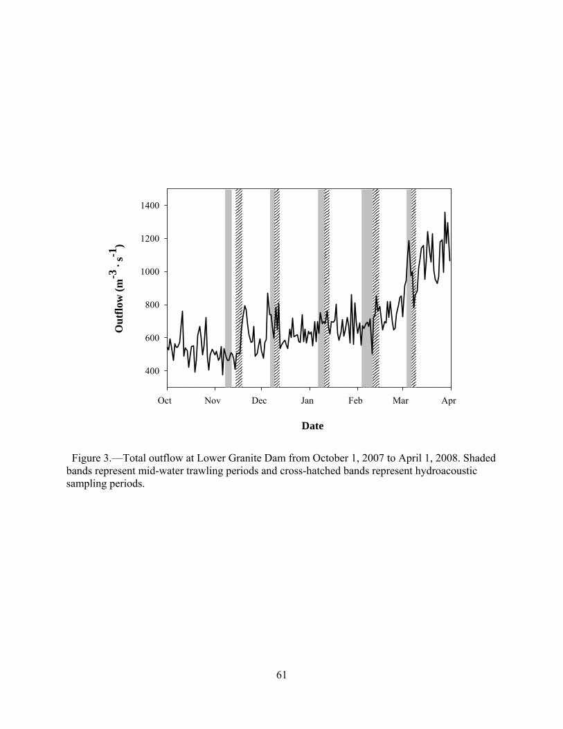
Date

Oct Nov Dec Jan Feb Mar Apr

Ou

tflo

w (

m-3

. s-1

)

400

600

800

1000

1200

1400

Figure 3.—Total outflow at Lower Granite Dam from October 1, 2007 to April 1, 2008. Shaded bands represent mid-water trawling periods and cross-hatched bands represent hydroacoustic sampling periods.

61

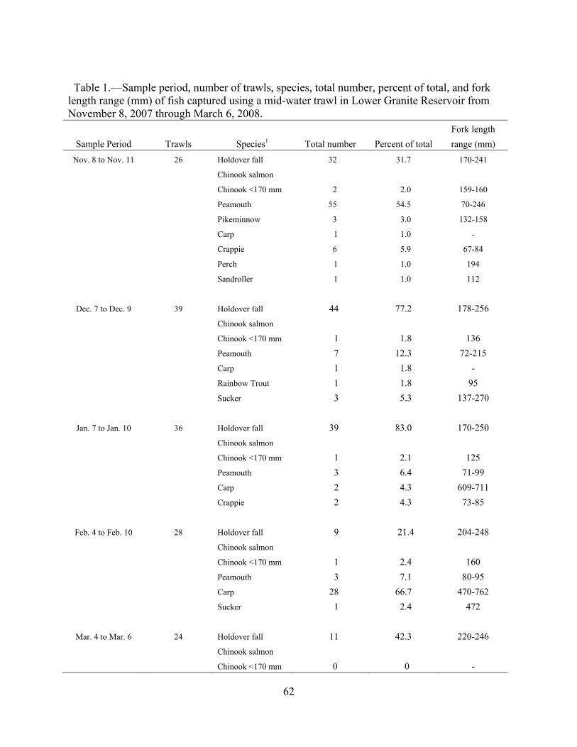
Table 1.—Sample period, number of trawls, species, total number, percent of total, and fork length range (mm) of fish captured using a mid-water trawl in Lower Granite Reservoir from November 8, 2007 through March 6, 2008.

Sample Period

Trawls

Species1

Total number

Percent of total

Fork length

range (mm)

Nov. 8 to Nov. 11 26 Holdover fall

Chinook salmon

32 31.7 170-241

Chinook <170 mm 2 2.0 159-160

Peamouth 55 54.5 70-246

Pikeminnow 3 3.0 132-158

Carp 1 1.0 -

Crappie 6 5.9 67-84

Perch 1 1.0 194

Sandroller 1 1.0 112

Dec. 7 to Dec. 9 39 Holdover fall

Chinook salmon

44 77.2 178-256

Chinook <170 mm 1 1.8 136

Peamouth 7 12.3 72-215

Carp 1 1.8 -

Rainbow Trout 1 1.8 95

Sucker 3 5.3 137-270

Jan. 7 to Jan. 10 36 Holdover fall

Chinook salmon

39 83.0 170-250

Chinook <170 mm 1 2.1 125

Peamouth 3 6.4 71-99

Carp 2 4.3 609-711

Crappie 2 4.3 73-85

Feb. 4 to Feb. 10 28 Holdover fall

Chinook salmon

9 21.4 204-248

Chinook <170 mm 1 2.4 160

Peamouth 3 7.1 80-95

Carp 28 66.7 470-762

Sucker 1 2.4 472

Mar. 4 to Mar. 6 24 Holdover fall

Chinook salmon

11 42.3 220-246

Chinook <170 mm 0 0 -

62

Table 1. Continued

Peamouth 12 46.2 80-288

Carp 1 3.8 660

Smallmouth Bass 1 3.8 272

Adult Steelhead 1 3.8 864

Overall 153 Holdover fall

Chinook salmon

135 50.0 170-256

Chinook <170 mm 5 3.7 125-160

Holdover fall

Chinook salmon

80 29.3 70-288

Carp 33 12.1 470-762

Crappie 8 2.9 67-85

Sucker 4 1.5 137-472

Pikeminnow 3 1.1 132-158

Rainbow Trout 1 0.4 85

Perch 1 0.4 194

Adult Steelhead 1 0.4 864

Smallmouth Bass 1 0.4 272

Sandroller 1 0.4 112

Table 2.—Sample period, mean water temperature (ºC), number of fall Chinook >170 mm, mean (±SD) fork length, mean (±SD) condition factor (K), and mean (±SD) abundance (fish/105 m3) of juvenile fall Chinook salmon (>170 mm) collected from mid-water trawls in Lower Granite Reservoir from November 8, 2007 through March 6, 2008.

Sample period

Mean

water

temp.

(ºC)

Number

of fall

Chinook

Mean

fork

length

(mm)

Mean

condition

factor

(K)

Mean

abundance

(fish/105 m3)

Nov. 8 to Nov. 11 9.6 31 218.3 ± 17.8 1.24 ± 0.105 18.60 ± 23.77

Dec. 7 to Dec. 9 5.7 44 220.6 ± 216 1.16 ± 0.096 19.04 + 24.11

Jan. 7 to Jan. 10 3.9 38 218.6 ± 20.4 1.12 ± 0.073 17.23 ± 25.98

Feb. 4 to Feb. 10 3.0 9 224.1 ± 16.4 1.08 ± 0.038 4.92 ± 9.36

Mar. 4 to Mar. 6 5.0 11 231.6 ± 8.9 1.11 ± 0.071 7.24 + 11.35

Overall 5.1 133 220.6 ± 19.4 1.16 ± 0.101 14.01 ± 21.47

63

of holdover juvenile fall Chinook salmon collected during each sample period was low, ranging from 44 fish from 39 trawls in December 2007 to 9 fish from 28 trawls in February 2008 (Table 2).

Peamouth was the primary fish species that overlapped in size with holdover fall Chinook salmon. Chinook salmon that we classified as holdovers ranged in size from 170 to 256 mm whereas peamouth sizes ranged from 70 to 288 mm. All other fish taxa were generally smaller or larger than holdovers. To apportion our acoustic targets by species, we determined the percentage of each potentially overlapping species (based on size) in our total trawl catch. Our small sample sizes precluded partitioning catches at a finer temporal scale. Therefore, of the 167 total fish collected within the size range exhibited by holdover fall Chinook salmon, 86.0 % (135 of 157) was holdovers, 12.7% was peamouth, 0.7% was unidentified catostomids, and 0.6% was yellow perch. We applied these percentages to our acoustic targets to ultimately extrapolate the number of holdover fall Chinook salmon in Lower Granite Reservoir. The lengths of fish collected by mid-water trawling were generally similar to those estimated from hydroacoustic target strengths using Love’s equation (Figure 4). Hydroacoustic surveys During each monthly sampling period, we completed 61 mobile hydroacoustic transects from November 2007 to February 2008. In March 2008 we were only able to complete 48 transects due to rough sampling conditions. We ensonified 5.38 to 7.66% of the entire reservoir volume during individual sampling periods using our combination of a 6º side-looking transducer and a 15º down-looking transducer for hydroacoustic sampling (Table 3). Overall, we enumerated 414 to 638 holdover fall Chinook salmon in Lower Granite Reservoir during monthly hydroacoustic surveys. When extrapolated to the whole volume of the reservoir, we estimated the number of holdover fall Chinook salmon to range from 6,180 fish in January 2008 to 11,697 fish in December 2007 (Table 3). Sampling error for our hydroacoustic surveys ranged from 878 in November 2007 to 2,138 in February 2008 (Table 3).

Mean abundance of holdover fall Chinook salmon estimated from hydroacoustic surveys

(range 1.15 to 2.19 fish/105 m3) was generally a magnitude less than that estimated from mid-water trawls (range 4.92 to 19.04 fish/105 m3; Table 4). Our highest monthly population estimate was in December 2007 (11,697, 90% CI = 7,573 to 15,821) and our lowest monthly population estimate was in January 2008 (6,180, 90% CI = 4,923 to 7,437). Trawling abundance estimates indicated that holdovers were more abundant closer to Lower Granite Dam and decreased with increasing distance upstream from the dam. However, hydroacoustic fish densities were generally greatest in the middle section of the reservoir, but exhibited no distinguishable trend (Figure 5).

64

Length (mm)

0 200 400 600 800 1000

Fre

quen

cy (

%)

0

2

4

6

8

10

12

Trawl Catch (n=273)Hydroacoustic Targets (n = 1,873)

Figure 4.—Comparison of fish lengths from holdover fall Chinook salmon collected with a mid-water trawl and those estimated from dorsal aspect target strengths filtered to include targets which fell within ±3º of the transducer axis. Target strengths from hydroacoustic surveys were converted to lengths using the empirical formula of Love (1971). Hydroacoustic surveys and mid-water trawls were conducted from November 2007 to March 2008 in Lower Granite Reservoir, Snake River. Table 3.—Sample period, total volume ensonified (m3), percent of reservoir volume ensonified, estimated number of juvenile fall Chinook salmon holdovers ensonified, hydroacoustic population estimate, and estimated sampling error following Aglen (1983).

Sample period

Volume

ensonified

(m3)

Percent of

reservoir

volume

ensonified

Estimated

number of

holdovers

ensonified

Population

estimate

Sampling

error

Nov. 15 to Nov. 18 32,385,368 6.04 543.88 9,855 878

Dec. 10 to Dec. 12 35,794,832 6.69 623.92 11,697 1,087

Jan. 10 to Jan. 13 36,888,287 6.89 414.10 6,180 1,110

Feb. 11 to Feb. 14 41,024,143 7.66 637.74 11,453 2,138

Mar. 6 to Mar. 9 28,810,421 5.38 434.57 8,648 1,321

65

Table 4.—Sample period, confidence level, estimated mean transect abundance, population estimate, t statistic, confidence interval, percent confidence interval, and population range of juvenile Chinook salmon holdovers estimated from hydroacoustic surveys conducted in Lower Granite Reservoir, Snake River from November 15, 2007 through March 9, 2008.

Sample period

Confidence

level

Mean

abundance

(# . 105 m3)

Population

estimate

t

stat

Confidence

interval

Percent

confidence

interval

Population

range

Nov. 15 to Nov. 18 1.841 9,855

99% 2.660 5,542 56.23 4,313-15,397

95% 2.000 4,167 42.28 5,689-14,022

90% 1.671 3,481 35.32 6,374-13,337

85% 1.484 3,092 31.37 6,764-12,947

80% 1.296 2,700 27.40 7,155-12,556

Dec. 10 to Dec. 12 2.185 11,697

99% 2.660 6,565 56.12 5,132-18,261

95% 2.000 4,936 42.20 6,761-16,633

90% 1.671 4,124 35.26 7,573-15,821

85% 1.484 3,662 31.31 8,034-15,359

80% 1.296 3,198 27.34 8,498-14,895

Jan. 10 to Jan. 13 1.154 6,180

99% 2.660 2,001 32.38 4,179-8,181

95% 2.000 1,505 24.35 4,675-7,685

90% 1.671 1,257 20.34 4,923-7,437

85% 1.484 1,117 18.07 5,064-7,297

80% 1.296 975 15.78 5,205-7,155

Feb. 11 to Feb. 14 2.139 11,453

99% 2.660 6,502 50.65 4,951-17,955

95% 2.000 4,889 38.08 6,564-16,342

90% 1.671 4,084 31.82 7,369-15,537

85% 1.484 3,627 28.26 7,826-15,080

80% 1.296 3,168 24.68 8,285-14,621

Mar. 6 to Mar. 9 1.615 8,648

99% 2.685 2,768 32.01 5,880-11,416

95% 2.012 2,074 23.99 6,574-10,722

90% 1.678 1,730 20.00 6,918-10,378

85% 1.489 1,535 17.75 7,113-10,183

80% 1.300 1,340 15.50 7,308-9,988

66

Distance from lower Granite Dam (kilometers)

0 10 20 30 40 50

Abu

ndan

ce (

num

ber

. 10,

000

m-3

)

0.0

0.2

0.4

0.6

0.8

Hydroacoustics0.0

1.0

2.0

3.0

4.0

5.0

6.0

7.0Trawling

Too shallowfor Trawling

Figure 5.—Mean (SE) holdover fall Chinook salmon density from five hydroacoustic surveys (top panel) and mid-water trawling (bottom trawling) surveys conducted in Lower Granite Reservoir from November 15, 2007 to March 19, 2008.

67

Discussion Our trawling data indicated that holdover fall Chinook salmon are likely more abundant and in better condition in late fall and early winter when water temperatures are higher than in late winter and early spring. However, all sample periods had mean condition factors greater than 1.0, indicating that they were in good condition to migrate in the spring. These results are not unexpected because fish probably do not feed and grow as much during winter months when temperatures are cold. We did not extrapolate abundances calculated from mid-water trawling because we only sampled the deeper portion of the water column with the trawl where we expected the trawl to be most effective. We anticipated small numbers of holdovers within our study area, and the number of fish we captured using the mid-water trawl was very low. We captured a total of 140 juvenile Chinook salmon, and 133 other fish from 153 mid-water trawls during five sample periods. These low numbers made the extrapolation of trawl fish composition and length frequencies to hydroacoustic files for individual sample periods questionable. Further, we were restricted to sampling a certain depth strata (9-12 m) using the mid-water trawl because sampling higher in the water column produced no fish and sampling deeper in the water column produced fewer fish and increased the probability that we would snag the trawl on the bottom of the river. Hydroacoustic data files indicated that many fish were higher in the water column. It is likely that we did not capture many fish using the mid-water trawl higher in the water column due to avoidance of the boat, prop wash, or lights in an otherwise dark environment. In 2007-2008, we sampled one depth strata to catch the most target fish possible while sacrificing our ability to describe trawl-caught fish abundance.

We recognize the limitations and biases our trawling strategy had on accurately characterizing the fish community and confirming targets in Lower Granite Reservoir. Consequently, our results should be viewed as preliminary and used cautiously. In 2008-2009 we plan to improve the accuracy of our target verification by using a lampara seine to collect fish. Our lampara seine is 228.60 m (750 ft) long and has the advantage of fishing the whole water column to a depth of 30.48 (100 ft). This will eliminate the depth-related bias inherent in our past trawling efforts. The lampara seine is fished by encircling a large area and then spooling the net back onto hydraulically powered drums. We believe that this net will not only allow us to catch more fish, but allow us to sample the entire water column with an individual net haul in both shallow and deep areas of the reservoir. Furthermore, we believe more species will be recruited to the gear and that larger fish will be less likely to avoid the net. From initial sampling with the lampara seine in October of 2008, we captured 299 fish, including 139 juvenile Chinook salmon from 70 seine hauls in Lower Granite and Little Goose reservoirs. Given our success of catching holdover fall Chinook salmon in Little Goose Reservoir we will expand our hydroacoustic and seining sampling to Little Goose as well as Lower Granite Reservoir in 2008 and 2009.

We estimated that the number of juvenile Chinook salmon residing in Lower Granite Reservoir during winter months ranged from 6,010 to 9,332 fish during 2007-2008. These are the first empirical estimates of holdover fall Chinook salmon abundances. Although monthly estimates were variable, the variations were not extreme. The relative consistency of our abundance estimates suggest that many fish resided in Lower Granite Reservoir the entire winter, however some fish likely passed the dam as shown by Kock et al. (2007). In an earlier attempt

68

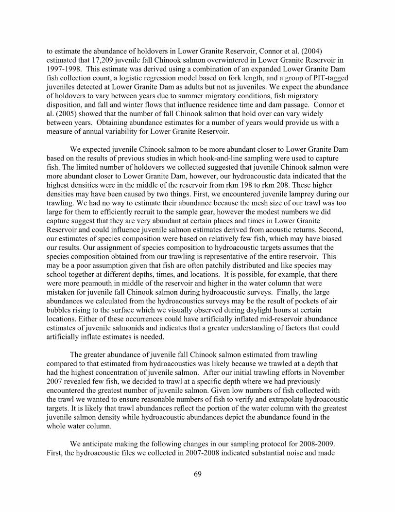
to estimate the abundance of holdovers in Lower Granite Reservoir, Connor et al. (2004) estimated that 17,209 juvenile fall Chinook salmon overwintered in Lower Granite Reservoir in 1997-1998. This estimate was derived using a combination of an expanded Lower Granite Dam fish collection count, a logistic regression model based on fork length, and a group of PIT-tagged juveniles detected at Lower Granite Dam as adults but not as juveniles. We expect the abundance of holdovers to vary between years due to summer migratory conditions, fish migratory disposition, and fall and winter flows that influence residence time and dam passage. Connor et al. (2005) showed that the number of fall Chinook salmon that hold over can vary widely between years. Obtaining abundance estimates for a number of years would provide us with a measure of annual variability for Lower Granite Reservoir. We expected juvenile Chinook salmon to be more abundant closer to Lower Granite Dam based on the results of previous studies in which hook-and-line sampling were used to capture fish. The limited number of holdovers we collected suggested that juvenile Chinook salmon were more abundant closer to Lower Granite Dam, however, our hydroacoustic data indicated that the highest densities were in the middle of the reservoir from rkm 198 to rkm 208. These higher densities may have been caused by two things. First, we encountered juvenile lamprey during our trawling. We had no way to estimate their abundance because the mesh size of our trawl was too large for them to efficiently recruit to the sample gear, however the modest numbers we did capture suggest that they are very abundant at certain places and times in Lower Granite Reservoir and could influence juvenile salmon estimates derived from acoustic returns. Second, our estimates of species composition were based on relatively few fish, which may have biased our results. Our assignment of species composition to hydroacoustic targets assumes that the species composition obtained from our trawling is representative of the entire reservoir. This may be a poor assumption given that fish are often patchily distributed and like species may school together at different depths, times, and locations. It is possible, for example, that there were more peamouth in middle of the reservoir and higher in the water column that were mistaken for juvenile fall Chinook salmon during hydroacoustic surveys. Finally, the large abundances we calculated from the hydroacoustics surveys may be the result of pockets of air bubbles rising to the surface which we visually observed during daylight hours at certain locations. Either of these occurrences could have artificially inflated mid-reservoir abundance estimates of juvenile salmonids and indicates that a greater understanding of factors that could artificially inflate estimates is needed. The greater abundance of juvenile fall Chinook salmon estimated from trawling compared to that estimated from hydroacoustics was likely because we trawled at a depth that had the highest concentration of juvenile salmon. After our initial trawling efforts in November 2007 revealed few fish, we decided to trawl at a specific depth where we had previously encountered the greatest number of juvenile salmon. Given low numbers of fish collected with the trawl we wanted to ensure reasonable numbers of fish to verify and extrapolate hydroacoustic targets. It is likely that trawl abundances reflect the portion of the water column with the greatest juvenile salmon density while hydroacoustic abundances depict the abundance found in the whole water column.

We anticipate making the following changes in our sampling protocol for 2008-2009. First, the hydroacoustic files we collected in 2007-2008 indicated substantial noise and made

69

target tracking of fish laborious. We believe that by switching our data collection frequency for active acoustics from 420 kHz to 200 kHz we can reduce the amount of noise in fish files, which will allow the auto-tracking software to perform better and reduce manual target tracking. Second, as previously mentioned, we will collect fish for target verification using a lampara seine to reduce the biases and limitations associated with trawling. Finally, we will also sample Little Goose Reservoir to increase our understanding of holdovers there. Kock et al. (2007) showed that fish that pass Lower Granite Dam during the winter also reside for extended periods in Little Goose Reservoir.

For 2008-2009 data analyses, we will achieve more refined estimates of both reservoir

volume and volume sampled. Recently collected, detailed bathymetry now exists that will allow us to more accurately define reservoir volume relative to the 1963 reservoir storage capacity curves that we used for analysis of 2007-2008 data. Additionally, we can refine estimates of volume sampled from the side-looking transducer. In 2007-2008, we multiplied the Great Circle Length transect distance by the conical area to a standard distance from the transducer of 60 m. In some cases however, the side-looking transducer beam was partially obstructed by the river bottom when depth was shallow. For 2008-2009 data analyses, we will construct additional data programs to further refine the volume sampled estimate from the side-looking transducer.

70

References Aglen, A. 1983. Random errors of acoustic fish abundance estimates in relation to the survey

grid density applied. FAO Fisheries Report 300:293-298. Anderson, R. O., and R. M. Neumann. 1996. Length, weight, and associated structural indices.

Pages 447-482 in B. R. Murphy and D. W. Willis, editors. Fisheries Techniques. American Fisheries Society, Bethesda, Maryland.

Arnsberg, B. D., and D. P Statler. 1995. Assessing summer and fall Chinook salmon restoration

in the upper Clearwater River and principal tributaries. Nez Perce Tribe Department of Fisheries Resources Management 1994 Annual Report to the Bonneville Power Administration, Project 1983350003, Portland, Oregon.

Arnsberg, B. D., D. S. Kellar, and M. A. Tuell. 2009. Nez Perce Tribal Hatchery monitoring

and evaluation of fall Chinook salmon supplementation in the Clearwater River Subbasin. 2007 Annual Report to the Bonneville Power Administration, Project 1983350003, Portland, Oregon.

Connor, W. P., H. L. Burge, R. Waitt, and T. C. Bjornn. 2002. Juvenile life history of wild fall

Chinook salmon in the Snake and Clearwater rivers. North American Journal of Fisheries Management 22:703-712.

Connor, W. P., K. F. Tiffan, J. G. Sneva, D. Ross, and R. K. Steinhorst. 2004. Fork length,

condition factor, and abundance of reservoir-overwintered fall Chinook salmon juveniles in the Snake River. Pages 40-55 in W. P. Connor, K. F. Tiffan, and J. G. Sneva, editors. Investigating passage of ESA-listed juvenile fall Chinook salmon at Lower Granite Dam during winter when the bypass system is not operated. 2003 Annual Report to the Bonneville Power Administration, Project Number 200203200, Portland, Oregon. Available online at: http://www.efw.bpa.gov/searchpublications.

Connor, W. P., J. G. Sneva, K. F. Tiffan, R. K. Steinhorst, and D. Ross. 2005. Two alternative

juvenile life history types for fall Chinook salmon in the Snake River Basin. Transactions of the American Fisheries Society 134:291-304.

Healey, M. C. 1991. Life history of Chinook salmon (Oncorhynchus tshawytscha). Pages 312 to

393, in C. Groot and L. Margolis, editors, Pacific salmon life histories. UBC press, Vancouver, British Columbia.

Kock, T. J., K. F. Tiffan, and W. P. Connor. 2007. Investigating the passage of ESA-listed

juvenile fall Chinook salmon at Lower Granite Dam during winter when the bypass system is not operated. Final Report by the U.S. Geological Survey to the Bonneville Power Administration, Project Number 200203200, Portland, Oregon. Available online at: http://www.efw.bpa.gov/searchpublications.

71

Love, R. H. 1971. Dorsal aspect target strength of an individual fish. Journal of the Acoustic

Society of America 49:816-823. Muir, W. D., S. G. Smith, J. G. Williams, and B. P. Sandford. 2001. Survival of juvenile

salmonids passing through bypass systems, turbines, and spillways with and without flow deflectors at Snake River dams. North American Journal of Fisheries Management 21:135-146.

NMFS (National Marine Fisheries Service). 1992. Threatened status for Snake River spring/summer Chinook salmon, threatened status for Snake River fall Chinook salmon. Federal Register 57:78 (22 April 1992):14653-14663.

Pope, K. L., and C. G. Kruse. 2007. Condition. Pages 423-471 in C. S. Guy and M. L. Brown, editors. Analysis and interpretation of freshwater fisheries data. American Fisheries Society, Bethesda, Maryland.

Simmonds, J., and D. MacLennan. 2005. Fisheries Acoustics: theory and practice, 2nd edition.

Blackwell Science, Oxford, UK. Tiffan, K. F., T. J. Kock, C. A. Haskell, W. P. Connor, and R. K. Steinhorst. 2009. Water

velocity, turbulence, and migration rate of subyearling fall Chinook salmon in the free-flowing and impounded Snake River. Transactions of the American Fisheries Society 138:373-384.

Zar, J.H. 1999. Biostatistical Analysis (Fourth edition). Prentice Hall, Englewood Cliffs, New

Jersey.

72

APPENDIX A

Assessment of the Effect of Delayed Migration on Estimates of the Joint Probability of Migration and Survival of Juvenile Fall Chinook Salmon to Lower Granite Dam

Rebecca A. Buchanan Columbia Basin Research

School of Aquatic and Fishery Sciences University of Washington

1325 Fourth Avenue, Suite 1820 Seattle, WA 98101

Introduction The objective of the sensitivity analysis was to assess the effect of delayed migration on estimates of the joint probability of migration and survival

to Lower Granite Dam. Large-

scale monitoring studies typically use PIT-tag detections to measure migration and survival. In the presence of delayed migration to Lower Granite Dam that results in smolt passage occurring after the end of PIT-tag operations, migration and survival estimates based on PIT-tag detections will be biased. One method of exploring the size and nature of this bias is to compare estimates of survival to Lower Granite Dam using two sets of detections: one set from an “abbreviated” detection period that corresponds to the usual period when the PIT-tag system was operational, and a second set from an “extended” period that includes additional weeks of detections. In 2007, PIT-tag detections at Lower Granite were available only during the abbreviated period, which ended at 1 November. Thus, it was not possible to estimate survival using PIT-tag detections from the extended detection period. The small numbers of fish released in this study also precluded using PIT-tag detections to estimate survival to Lower Granite in the abbreviated period. For these reasons, it was necessary to use acoustic-tag detections to estimate survival to Lower Granite Dam for both detection periods. Unlike PIT-tag detections, which yield estimates of survival to the tailrace, detections from the five acoustic arrays used in this study yield estimates of survival to the forebay. Nevertheless, if the acoustic-based survival estimates to the Lower Granite Dam forebay are different for the abbreviated and extended detection periods, we can conclude that estimates of survival to the tailrace that are based on PIT-tag detections from the typical (“abbreviated”) PIT-tag detection season would be biased.

Statistical Methods

For each acoustic-tag release group (see Section B.2.1), detection histories were formed for the “abbreviated” detection period, and separately for the “extended” detection period. The abbreviated period ended when the PIT-tag detection system usually shuts down at the Snake River dams. In 2007, the PIT-tag detection system shut down on different dates at different dams. For simplicity, the usual shut-down date of 1 November 2007 was used as the end of the

73

abbreviated period. The end of the extended period depended on the release group and the tag-life of the tags used. The acoustic tags used in this study varied in tag life, with 60-day tags used for the first 2 releases, and 120-day tags used in the last release. The first release group of acoustic-tagged fish was released in August, and the 60-day tags were expected to fail before 1 November 2007, so this release group was not used in the sensitivity analysis. The second release group also used 60-day tags, with the expectation that the tags would last at least until 17 November 2007. The tag-life study indicated that the 60-day tags lasted considerably longer than 60 days (mean observed tag life = 90 days), so the 17 November 2007 end-date for the extended period for release 2 was deemed reasonable ( Table 1). The third release group used 120-day tags, and were not expected to fail before 14 February 2008; this date was used as the cut-off date of the extended period for the third release group ( Table 1). Cut-off dates were non-inclusive. Table 1.—Abbreviated and extended detection periods for release groups of acoustic-tagged subyearling Chinook salmon used in 2007 sensitivity analysis. * = Release group 1 was not used in the sensitivity analysis, because its entire detection period was completely contained within the abbreviated period. Ending dates of detection periods were non-inclusive.

Release Group

Release Date

Tag Life Abbreviated Period Extended Period

1* 18 Aug. 2007

60 days 18 Aug. 2007 – 17 Oct. 2007

NA

2 18 Sept. 2007

60 days 18 Sept. 2007 – 1 Nov. 2007

18 Sept. 2007 – 17 Nov. 2007

3 17 Oct. 2007

120 days

17 Oct. 2007 – 1 Nov. 2007

17 Oct. 2007 – 14 Feb. 2008

For each release group, the joint probability of migrating and surviving from the release point to the LGR forebay was estimated for both the abbreviated detection period A and for

the extended detection period E using the methods described in Section B.2.2. A one-sided

-test was used to test the hypothesis that the migration and survival probability from the extended period was greater than the corresponding probability from the abbreviated period, i.e., t

H : E AA .

Results

For both release groups 2 and 3, there were insufficient detections at the LGR forebay and tailrace arrays during the abbreviated detection period to generate estimates of the joint probability of migration and survival to the LGR forebay during that detection period. However, for both release groups it was possible to estimate the migration and survival probability to the LGR forebay using detections from the extended detection period (

74

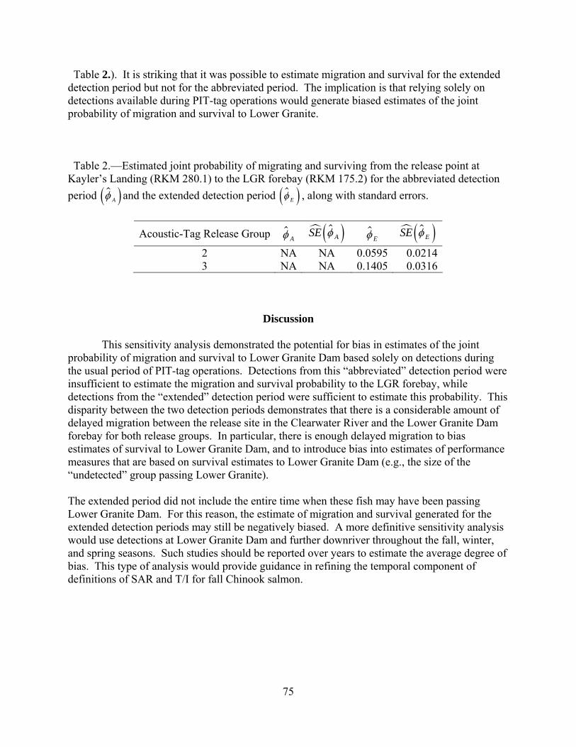
Table 2.). It is striking that it was possible to estimate migration and survival for the extended detection period but not for the abbreviated period. The implication is that relying solely on detections available during PIT-tag operations would generate biased estimates of the joint probability of migration and survival to Lower Granite. Table 2.—Estimated joint probability of migrating and surviving from the release point at Kayler’s Landing (RKM 280.1) to the LGR forebay (RKM 175.2) for the abbreviated detection

period A and the extended detection period E , along with standard errors.

Acoustic-Tag Release Group A ASE

E ESE

2 NA NA 0.0595 0.0214 3 NA NA 0.1405 0.0316

Discussion This sensitivity analysis demonstrated the potential for bias in estimates of the joint probability of migration and survival to Lower Granite Dam based solely on detections during the usual period of PIT-tag operations. Detections from this “abbreviated” detection period were insufficient to estimate the migration and survival probability to the LGR forebay, while detections from the “extended” detection period were sufficient to estimate this probability. This disparity between the two detection periods demonstrates that there is a considerable amount of delayed migration between the release site in the Clearwater River and the Lower Granite Dam forebay for both release groups. In particular, there is enough delayed migration to bias estimates of survival to Lower Granite Dam, and to introduce bias into estimates of performance measures that are based on survival estimates to Lower Granite Dam (e.g., the size of the “undetected” group passing Lower Granite). The extended period did not include the entire time when these fish may have been passing Lower Granite Dam. For this reason, the estimate of migration and survival generated for the extended detection periods may still be negatively biased. A more definitive sensitivity analysis would use detections at Lower Granite Dam and further downriver throughout the fall, winter, and spring seasons. Such studies should be reported over years to estimate the average degree of bias. This type of analysis would provide guidance in refining the temporal component of definitions of SAR and T/I for fall Chinook salmon.

75

APPENDIX B

Fall Chinook Salmon SAR Estimation and Bias Correction

Rebecca A. Buchanan John R. Skalski

Columbia Basin Research School of Aquatic and Fishery Sciences

University of Washington 1325 Fourth Avenue, Suite 1820

Seattle, WA 98101

Introduction The SAR (smolt-to-adult return ratio) is the probability of a salmonid returning to Lower Granite Dam as an adult, conditional on reaching Lower Granite Dam as a juvenile. It is a measure of the overall migration success through the hydrosystem for a release group or brood year, and is an important performance measure used in fishery and hydrosystem management. The Comparative Survival Study (CSS; Schaller et al. 2007) attempts to estimate SAR for non-detected fish, that is, for fish that passed dams as juveniles without using the juvenile bypass systems at the four transport dams. The CSS estimator of SAR depends on estimation of the survival probability to Lower Granite and of the detection probabilities at the transport dams. Fall Chinook salmon smolts may complete their juvenile outmigration in the summer or fall of their first year (i.e., as subyearlings), or in the following winter or spring. Fish that migrate out during their first fall exhibit an “ocean life history” (OLH), while fish that complete migration during the winter or spring following their first fall exhibit a “reservoir life history” (RLH). There is concern that the CSS methods to estimate SAR produce biased estimates when used with PIT-tag detection data from fall Chinook salmon, because of the alternative reservoir life history exhibited by some fall Chinook. In particular, the adults used to estimate SAR will include both ocean life-history fish and reservoir life-history fish, while the juveniles used in estimation will include only ocean life-history fish. This is because smolts that migrate during the winter, when the PIT-tag system is not operational, go undetected. This disparity between juveniles and adults has prompted a desire for a fall Chinook bias correction to the SAR estimator used by the CSS. The objective of this chapter is to define and develop statistical methods for estimating this bias correction.

SAR Estimators The SAR is typically estimated as the ratio of the number of adults detected at Lower Granite A to the number of juveniles that passed Lower Granite J , for a given release group:

76

ASAR

J .

For inference specifically to undetected fish, the number of adults used to estimate SAR is limited to those adults that were not detected at any of the four transport dams as juveniles 0A .

The number of juveniles is typically represented in terms of “Lower Granite equivalents”,

or the number of juveniles that must have passed Lower Granite Dam that were “destined” to have a particular downstream detection history, if survival from Lower Granite Dam were 100%. Thus, is the number of juveniles from a release group that passed Lower Granite Dam that

were “destined” to pass all transport dams undetected, if they had all survived to those dams. The number must be estimated because it reflects what “would have happened” in the

hypothetical situation of 100% survival, and because by definition, none of the smolts it represents were detected at either Lower Granite Dam or the other transport dams. Thus, the estimator of SAR limited to undetected fish is:

0J

0J

0J

0

0

ASAR

J .

The estimator used in the CSS reports has the following form (Schaller et al. 2007):

0

0,

CSS

CSS

ASAR

J ,

where is the estimated number of juveniles that must have passed Lower Granite that were “destined” to pass all transport dams undetected. Additionally, the CSS estimator of (and of

SAR) censors all smolts that were removed from the migration downstream of McNary (e.g., in sampling rooms at downstream dams).

0,CSSJ

0J

The adjusted SAR estimator developed here ADJSAR differs from CSSSAR by adjusting

the estimator of in the denominator: 0J

0

0, 0,

ADJ

CSS RLH

ASAR

J J

,

where 0,RLHJ is the estimated number of juveniles that passed Lower Granite that were “destined” both to adopt a reservoir life history (RLH) before passing Bonneville, and to pass the

transport dams undetected. The number 0,RLHJ excludes smolts “destined” to be removed from the migration downstream of McNary. The adjusted SAR estimator may also be expressed as the following:

ADJ CSSSAR SAR ,

where is a multiplicative bias correction of the form

0,

0,

1.

1RLH

CSS

J

J

77

It will be shown in this document that (or alternatively, 0,RLHJ ) is a complex function of numerous parameters, rather than a single, simple value. Notation Detection sites 1, ,6i i are indexed as follows:

Site 1 = release site Site 2 = Lower Granite Dam (LGR) Site 3 = Little Goose Dam (LGS) Site 4 = Lower Monumental Dam (LMO) Site 5 = Ice Harbor Dam (ICH) Site 6 = McNary Dam (MCN) Reaches 1, ,6i i are indexed: Reach 1 = release site to Lower Granite; Reach 2 = Lower

Granite to Little Goose; etc., Reach 6 = McNary to John Day Dam. Parameters are classified by season: “F” = fall or summer of release year; “W” = winter following the fall of the release year; and “S” = spring following the release year. Define the following parameters: R = size of release group (release made in summer or fall upstream of LGR) iF = joint probability of migration and survival through reach i in the fall (or summer) of

the release year, for 1, ,6i iW = joint probability of migration and survival through reach i in the winter following

the fall of the release year, for 1, ,6i iS = joint probability of migration and survival through reach i in the spring following

the release year, for 1, ,6i F

iW = joint probability of residualizing in reach i from fall to winter, and migrating and

surviving through reach i in winter, for 1, ,6i

FiS = joint probability of residualizing in reach i from fall to spring, and migrating and

surviving through reach i in spring, for 1, ,6i

WiS = joint probability of residualizing in reach i from winter to spring, and migrating

and surviving through reach i in spring, for 1, ,6i

iFp = probability of being detected on PIT-tag detectors at site i , conditional on reaching

site i in the fall of the release year, for 2, ,6i

1 p = probability of passing site i undetected, conditional on reaching site i in

the fall of the release year, for iF iFq

2, ,6i iWp = probability of being detected on PIT-tag detectors at site i , conditional on

reaching site i in the winter following the fall of the release year, for 2, ,6i

1 p = probability of passing site i undetected, conditional on reaching site i in

the winter following the fall of the release year, for iW iWq

2, ,6i

iSp = probability of being detected on PIT-tag detectors at site i , conditional on reaching

site i in the spring following the release year, for 2, ,6i

78

1 p = probability of passing site i undetected, conditional on reaching site i in

the spring following the release year, for 2, ,6iiS iSq

F = probability of being removed from migration (e.g., from sampling room)

downstream of McNary, as a juvenile in the fall of the release year W = probability of being removed from migration (e.g., from sampling room)

downstream of McNary, as a juvenile in the winter following the fall of the release year S = probability of being removed from migration (e.g., from sampling room)

downstream of McNary, as a juvenile in the spring following the release year. CSS Estimator of SAR

The CSS estimator of 0J 0,CSSJ is expressed in terms of the numbers of fish first

detected at each transport dam, the detection probability at Lower Granite, and the estimated survival probability to each dam (Schaller et al. 2007):

13 16 012 140, 12

2 2 2 3 2 3 4 5 2 3 4 5 6

CSSm m dm m

J mP S S S S S S S S S S S S

,

where

122

2 212

2

mP

Z am

r

= estimator of detection probability at LGR;

2Z = number of smolts detected downstream of LGR but not at LGR;

2a = number of smolts detected at LGR and returned to the river there;

2r = number of smolts detected at LGR and returned to the river there and then detected

downstream; 2S = CJS survival parameter from LGR to LGS (Cormack 1964; Jolly 1965; Seber

1965); 3S = CJS survival parameter from LGS to LMO;

4S = CJS survival parameter from LMO to IH;

5S = CJS survival parameter from IH to MCN;

0d = number of smolts removed downstream of MCN with no previous detections at

transport dams; 12m = number of smolts detected at LGR;

13m = number of smolts first detected at LGS (not detected at LGR);

= number of smolts first detected at LMO; 14m

= number of smolts first detected at MCN. 16m

The CJS parameters used in correspond to the iS 2, ,6i 0,CSSJ iF parameters defined

specifically for the fall Chinook salmon life history. The CSS estimator has the following expected value:

0,CSSJ

79

0, 1 2 3 4 5 1CSS F F F F F FE J R q q q q .

It is apparent that has inference only to ocean life-history fish. 0,CSSJ

Adjusted SAR Estimator

At first glance, it may seem reasonable to correct the bias in CSSSAR for fall Chinook salmon by restricting the count of adults in the numerator to those that entered saltwater as subyearlings. These adults may be identified using scale analysis of adults detected at Lower Granite Dam. However, 100% of the returning adults (that were undetected as juveniles) would need to be sampled for scale analysis. Additionally, the resulting SAR estimate would have inference only to ocean-type fall Chinook salmon, and would be biased for the combined population of reservoir-type and ocean-type fall Chinook.

The above considerations mean that in order to correct the bias in CSSSAR for fall Chinook salmon, it is necessary to adjust the estimated number of juveniles in the denominator. The CSS

estimator of 0J 0,CSSJ estimates the number of undetected OLH fish that passed Lower

Granite dam (i.e., those that passed LGR undetected in the fall and were “destined” to pass all other transport dams undetected in the fall). The approach to bias-correction taken here is to adjust the CSS estimator of so that it includes RLH fish, i.e., those fish that passed LGR

undetected in winter or spring, and were “destined” to pass all other transport dams undetected in winter or spring. The bias-correction allows for residualization that lasts throughout either part or all of the winter and that occurs anywhere throughout the juvenile migration. The adjusted estimator of is

0J

0J

, 0 0, 0,CSS RLHJ J J

where 0,RLHJ estimates the number of fish that passed Lower Granite undetected that were “destined” to pass the downstream transport dams undetected, avoid removal downstream of McNary, and enter the ocean in either the winter or spring following the year of release (i.e.,

exhibiting a reservoir life history). The adjusted SAR estimator, ADJSAR , is then

0

0, 0,

ADJ

CSS RLH

ASAR

J J

.

Whereas there is only a single migration path that may be taken by fish included in (i.e., passing all dams in the fall without detection), there are many paths that may be taken by the fish

that are counted in

0,CSSJ

0,RLHJ . For example, RLH fish may residualize to winter upstream of Lower

Granite, and then pass all dams in winter. Alternatively, RLH fish may pass Lower Granite in the fall, residualize to spring between Lower Granite and Little Goose, and then migrate past all downstream dams in the spring. A third possibility is to residualize until winter upstream of Lower Granite, pass Lower Granite and Little Goose in winter, then residualize until spring between Little Goose and Lower Monumental, and finally pass Lower Monumental and all downstream dams in spring. With the possibility of residualizing to either winter or spring in any of the 6 reaches, and the possibility of winter residualization followed by spring residualization, there are 27 possible migration paths that are represented by the RLH fish

counted by 0,RLHJ . Rather than writing out the estimator 0,RLHJ in terms of counts of fish at

80

each site in an analogy of the estimator , we instead present the expected value of 0,CSSJ

0,RLHJ

1

in terms of the parameters defined above:

0, 1 2 3 1 2 3 4 6

1 2 3 1 2 3 4 6

1 2 1 2 3 4 6

1 2 3 1 2 3 4 6

1 2 3

1 1

1 1

2 1

1 1

F FRLH S S S W W W W W W

F FW W S S W W W S S S

F FW W S S W W W W W S

F F S S F F W W W W

F F W

E J R q q q R q q q q

R q q R q q q q

R q q R q q q q

R q q R q q q q

R q q

4 6

4 6

3 4 6

4 6

4 6 1

S S S

S S

W W

S S

S S

q

q q

q q

q q

q q

1 2 3 4 6

1 2 3

1 2 3 1 2 3 4 6

1 2 3 1 2 3 4 6

1 2 1 2 3 4 6

1 2 3

1

2 1

1 1

2

S F F W W S

F F W S

F F F S F F F W W W

F F F S F F F W W S

F F S F F F F W W

F F S

R q q q q

R q q

R q q R q q q q

R q q R q q q q

R q q R q q q q

R q q

R

1

1

S

4 6

4 6

4 6

3 4 6

4 6

1

2 1

3 1

1

W W

S S

W S

F F S

F F W

q q

q q

q q

q q

q q

2 3 1 2 3 4 61 1F F S F F F F F Wq q R q q q q

4 6F F Fq q .

In the case where PIT-tag detection probabilities and removal probabilities in winter are 0 (i.e.,

, , and 0iWp 1iWq 0W ), the expression for 0,RLHE J is somewhat simplified to the

following:

0, 1 6 1

1 3 1 4 6

1 6 1

1 2 6 1 2

1 2 1 2 6

1 2

1 2 6 1 2 3

1

1 1

1

1

1 2

1

F FRLH S S S S W

F FW S W S S S

F FW S S W S

F F S S F F

F F S F F S S

F F

F F S S F F

E J R q R

R q R q q

R q R

R q q R q

R q R q q

R q

R q q R q q

2 3 4

4 6

3 4

4 6

3 4

2 1

1

S S

S S S

S S

S S

S

F S

q q q

q q

q q

q q

q q

1

1 2 1 2 3

1 2 6 1 2 3 4

1 2

1 2 6 1 2 3 4 6

2 1 1

3 1 2

1

1 .

F

F F S S F F F S

F F S S F F F F

F F S

F F F S F F F F F

R q R q q

R q q R q q q

R q

R q q R q q q q

3 6

3 4

3 4

3 4

F

F F

F F

F F

q q

q q

q q

q q

81

The expression for 0,RLH is a function of: E J

the detection probabilities at each site in each season (i.e., ,iF iWp p , and iSp );

the joint probability of migrating and surviving from the release site to LGR in the fall (or summer) of the release year 1F ;

the joint probability of residualizing upstream of LGR and migrating past LGR in either the winter 1

FW or spring 1

FS following the release year; and

the probability of being removed downstream of McNary in the winter W or spring

S following the release year.

The acoustic detection data from the 2007 study may be used to estimate 1F , the joint

probability of migrating and surviving from the release point to Lower Granite Dam in the fall of the release year. Estimation of the probabilities of residualizing and then migrating ( 1

FW and

1FS ) will require tags that last throughout winter and spring, respectively. Estimation of the

detection ( ,iF iWp p , and iSp ) and removal ( W and S ) probabilities may be performed using

PIT-tag data.

Design Implications Estimation of the bias-correction term requires estimating several types of

parameters over different seasons following release of fall Chinook salmon. The parameters are listed here by category (e.g., residualization, detection), and the study designs necessary for estimating them are described.

0,RLHJ

Detection Probabilities iFp = probability of being detected on PIT-tag detectors at site i , conditional on reaching

site i in the fall of the release year, for 2,3, 4,6i

iWp = probability of being detected on PIT-tag detectors at site i , conditional on

reaching site in the winter following the fall of the release year, for i 2,3, 4,6i

iSp = probability of being detected on PIT-tag detectors at site i , conditional on reaching

site in the spring following the release year, for i 2,3, 4,6i

If it is assumed that PIT-tag detections are unavailable during winter, then 0iWp for all sites.

PIT-tag detections should be available during the fall and spring seasons, however, so iFp and

iSp will need to be estimated. The iFp parameters may be estimated from PIT-tag detections

that are limited to the year of release (i.e., from the summer or fall of the release year) using the CJS model or the single-release model (Skalski et al. 1998). The iSp parameters may be

estimated from PIT-tag detections from the spring following the release year. The initial release of PIT-tagged subyearlings should be large enough that sufficient reservoir life-history fish survive to the following spring in order to estimate iSp for each transport dam.

82

Migration, Residualization, and Survival Parameters 1F = joint probability of migration and survival from the release site to Lower Granite in

the fall (or summer) of the release year 1

FW = joint probability of residualizing between the release site and Lower Granite from

fall to winter, and migrating and surviving to Lower Granite in winter 1

FS = joint probability of residualizing between the release site and Lower Granite from

fall to spring, and migrating and surviving to Lower Granite in spring The 1F parameter is equal to the CJS parameter , representing survival from release to Lower

Granite, when is estimated from PIT-tag detections that are limited to the year or release (i.e.,

no detections from winter or the following spring are used). The

1S

1S

1FS parameter can also be

estimated using PIT-tag data:

12

1

1

F SS

S

m

R p ,

where R is the size of the PIT-tagged release group (released in the previous year), is the

number of juveniles from that release group detected at Lower Granite the following spring, and 12Sm

1Sp is the PIT-tag detection probability of yearling fall Chinook smolts at Lower Granite in the

spring following the release year. Unlike the 1F and 1

FS parameters, the 1

FW parameter cannot be estimated using PIT-tag

data unless PIT-tag detections are available throughout the winter. Instead, estimation of 1FW

requires the use of long-lived tags that may be detected throughout the winter (i.e., throughout the period when the PIT-tag detection system is nonoperational at one or more of the transport dams). For example, long-lived acoustic tags may be used with a double array of acoustic receiving nodes in the Lower Granite tailrace. The double array will provide an estimate of acoustic-tag detection efficiency at the array ATp , yielding the following estimator of 1

FW :

12

1

F W AT

W

AT AT

m

R p ,

where ATR is the size of the release group of acoustic-tagged subyearlings, and is the

number of these acoustic-tagged fish detected on the double acoustic array in the Lower Granite tailrace during the winter following the fall of the release year.

12W ATm

Removal Parameters W = probability of being removed from migration (e.g., from sampling room)

downstream of McNary, as a juvenile in the winter following the fall of the release year S = probability of being removed from migration (e.g., from sampling room)

downstream of McNary, as a juvenile in the spring following the release year. If removal occurs only during periods of PIT-tag operations, then 0W . The S parameter

may be estimated using PIT-tag detections from the spring following the release year, analyzed using the CJS model with removals.

83

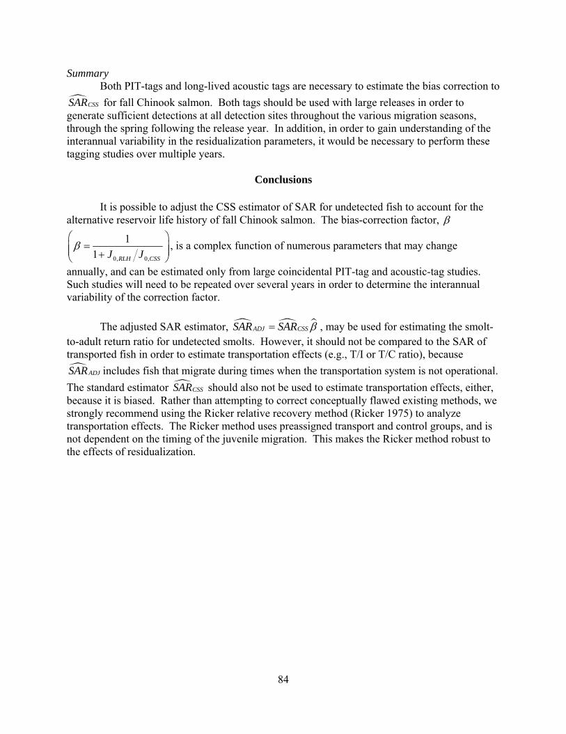
Summary Both PIT-tags and long-lived acoustic tags are necessary to estimate the bias correction to

CSSSAR for fall Chinook salmon. Both tags should be used with large releases in order to generate sufficient detections at all detection sites throughout the various migration seasons, through the spring following the release year. In addition, in order to gain understanding of the interannual variability in the residualization parameters, it would be necessary to perform these tagging studies over multiple years.

Conclusions It is possible to adjust the CSS estimator of SAR for undetected fish to account for the alternative reservoir life history of fall Chinook salmon. The bias-correction factor,

0, 0,

1

1 RLH CSSJ J

, is a complex function of numerous parameters that may change

annually, and can be estimated only from large coincidental PIT-tag and acoustic-tag studies. Such studies will need to be repeated over several years in order to determine the interannual variability of the correction factor.

The adjusted SAR estimator, ADJ CSSSAR SAR , may be used for estimating the smolt-

to-adult return ratio for undetected smolts. However, it should not be compared to the SAR of transported fish in order to estimate transportation effects (e.g., T/I or T/C ratio), because

ADJSAR includes fish that migrate during times when the transportation system is not operational.

The standard estimator CSSSAR should also not be used to estimate transportation effects, either, because it is biased. Rather than attempting to correct conceptually flawed existing methods, we strongly recommend using the Ricker relative recovery method (Ricker 1975) to analyze transportation effects. The Ricker method uses preassigned transport and control groups, and is not dependent on the timing of the juvenile migration. This makes the Ricker method robust to the effects of residualization.

84

85

References

Cormack, R.M. 1964. Estimates of survival from the sighting of marked animals. Biometrika 51:429-438.

Jolly, G.M. 1965. Explicit estimates from capture-recapture data with both death and

immigration – stochastic model. Biometrika 52:225-247. Ricker, W.E. 1975. Computation and interpretation of biological statistics of fish populations.

Bulletin of the Fisheries Research Board of Canada, 191, 382 p. Schaller, et al. 2007. Comparative Survival Study (CSS) of PIT-Tagged Spring/Summer

Chinook and Steelhead in the Columbia River Basin: Ten-Year Retrospective Analysis Report (Draft). Report to BPA, Contract # 19960200.

Seber, G.A.F. 1965. A note on the multiple recapture census. Biometrika 52:249-259. Skalski, J.R., S.G. Smith, R.N. Iwamoto, J.G. Williams, and A. Hoffmann. 1998. Use of PIT tags

to estimates survival of migrating juvenile salmonids in the Snake and Columbia Rivers. Canadian Journal of Fisheries and Aquatic Sciences 55:1484-1493.