snow drifting transport rates from water flume simulation

ARTICLE IN PRESS

Journal of Wind Engineering

and Industrial Aerodynamics 92 (2004) 1245–1264

0167-6105/$ -

doi:10.1016/j

�CorrespoE-mail ad

www.elsevier.com/locate/jweia

Snow drifting transport rates from waterflume simulation

Michael O’Rourkea,�, Arthur DeGaetanob,Janine Derjue Tokarczykc

aRensselaer Polytechnic Institute, Department of Civil and Environmental Engineering, 110 8th Street, Troy,

NY 12180-3590, USAbDepartment of Earth and Atmospheric Sciences, Cornell University, Ithaca, NY, USA

cSpiegel Zamecnik & Shah Inc., New Haven, CT, USA

Received 17 December 2003; received in revised form 2 August 2004; accepted 12 August 2004

Available online 17 September 2004

Abstract

The drift formation process consists of some of the snow blowing towards a geometric

irregularity being trapped. Analytical estimation of snow drift size requires both information

on the transport rate for snow blowing from a source area, as well as information on the

trapping efficiency of a particular geometric irregularity. Herein, laboratory simulation of the

snow drifting process using the Rensselaer Water Flume is described. Similitude relations are

presented which establish correspondence between the crushed walnut shell in water model of

the snow in air prototype.

It is shown that the scaled transport rates from the water flume models matches reasonably

well with full scale transport rates. This suggests that water flume simulation can be used for

quantitative evaluation of snow drifting.

r 2004 Elsevier Ltd. All rights reserved.

Keywords: Water flume procedures; Snow transport; Snow drifting; Simulation; Snow loading

see front matter r 2004 Elsevier Ltd. All rights reserved.

.jweia.2004.08.002

nding author. Tel.: +518-2766933; fax: +518-2764833.

dress: [email protected] (M. O’Rourke).

www.elsevier.com/locate/jweia

ARTICLE IN PRESS

M. O’Rourke et al. / J. Wind Eng. Ind. Aerodyn. 92 (2004) 1245–12641246

1. Introduction

In the past, snow load provisions in building codes have been based in large partupon full-scale case history measurements. This is perhaps most evident in snow driftrelations. For example, the current provisions in the ASCE 7 load standard for aleeward roof step snow drift (i.e. step with a upwind upper level roof) are takendirectly from an analysis of approximately 350 roof snow drift case histories byO’Rourke et al. [1]. Similarly, the three quarters modification factor used in relationto windward roof step drifts (i.e. step with a upwind lower level roof) is based uponan analysis of about a half dozen case histories by O’Rourke and DeAngelis [2].Case histories have also played a significant role in the development of uniform

roof snow load provisions. The uniform or balanced load provision in older versionsof ASCE 7 were based upon Canadian provisions which in turn were based uponcase histories by Schriever et al. [3] and Lutes and Schriever [4]. Similarly an analysisof simultaneous measurements of ground and roof snow loads by O’Rourke et al. [5]provide benchmarks for the exposure and thermal factors, Ce and Ct, in more recentversions of ASCE 7 while an analysis of more than a dozen case histories by Sack [6]provides a benchmark for the slope factor, Cs.A major advantage of case histories is that they are derived from measurements of

real snow on real buildings. As such, they provide readily believable justification forsnow provisions. Unfortunately, there are drawbacks with the case history approach.First of all, the process of gathering case histories is time consuming and requiresweather conditions over which the investigator has no control. Unlike laboratorytesting, case histories typically do not allow one to determine the influence of aparticular parameter by simply varying the parameter of interest while keeping allother parameters unchanged. Unlike laboratory testing, case histories typically donot allow one to determine the inherent variability of a process by simply rerunningthe same test. Also, the case history approach, by its nature, can not be used for aproposed one-of-a-kind structure. Most importantly, case histories typically recordsnow loading on a particular structure during a given winter as opposed tomonitoring the same structure over a number of winters. As such, case historiescannot be used to establish the return period for a particular magnitude of load.The earliest investigation of water flume simulation of snow drifting was

undertaken by Isyumov [7], in which he notes, ‘‘model techniques, if provenrepresentative, may prove valuable in the evaluation of snow loads’’. In practice,water flume simulation has been used primarily for qualitative evaluation of snowdrifts. A typical example is using flumes to determine where drifts might formaround a building so that entrances can be appropriately located. Herein,quantitative evaluation of snow drifting using the Rensselaer water flume will bepresented. That is, laboratory methods are used to estimate the size of a roof topdrift, not simply its location. Similitude relations developed by others are used todetermine the required diameter and density of the crushed walnut shells particleswhich model snow particles. The observed transport rate of walnut shells in theflume is found to compare favorably with the full-scale equivalent. This suggests thatwater flume simulation can be used for quantitative evaluation of snow drifting.

ARTICLE IN PRESS

M. O’Rourke et al. / J. Wind Eng. Ind. Aerodyn. 92 (2004) 1245–1264 1247

2. Rensselaer water flume equipment and procedures

As described more fully by Derjue [8], the Rensselaer water flume is an openchannel, 7.6m (25 f) in length, 0.76m (2.5 f) in width, having a total depth of 1.22m(4 f). A plan view of the Rensselaer flume is shown in Fig. 1.Water flows from the inlet area (sta. 0 to sta. 2 in Fig. 1) towards the outlet area

(stas. 23–25). The building model is located between stations 11 and 14. In order tosimulate a boundary layer flow, inverted triangular spines as suggested by Irwin [9],are located at station 2, while small bricks are located on the flume floor betweenstations 3 and 9. Upstream velocity is measured at station 9 using a SwofferInstruments model 2100 Current Velocity Meter.All the building models were at 1:30 geometric scale and were constructed of 2� 4

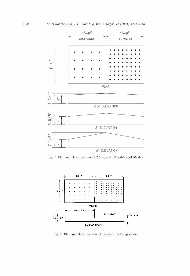
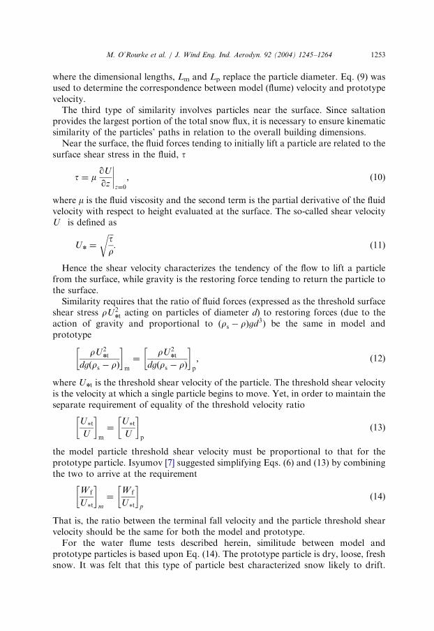
dimensional lumber and 1.27 cm (1/2 in.) plywood. Results from three separate roofgeometries are reported herein, specifically a symmetric gable roof with the ridge lineperpendicular to the direction of flow, a two-level roof with the upper level roofupstream of the lower level (i.e. leeward roof step), and a flat roof. Plan andelevation views of the gable roof models are shown in Fig. 2. Note that the roofslopes of 2.51, 51, and 101 approximate common roof slopes of 1/2 on 12, 1 on 12 and2 on 12. The roof step model is shown in Fig. 3. The flat roof model is similar, havinga cross-wind dimension of 61 cm (24 in.), a long wind dimension of 122 cm (48 in.)and a height of 10.2 cm (4 in.).For the gable roof tests, the total depth of water in the flume varied, depending on

roof slope, such that the model always had about 10.2 cm (4 in.) of water above theridge line. In the roof step tests, the total water depth was typically 30.5 cm (12 in.),while for the flat roof tests the water depth varied from 21.6 to 24.1 cm with thesmaller depth being associated with slower water velocities. In all cases, the waterdepth was established by varying the height of the baffles at the outlet end of thewater flume.For most all tests described herein, it was assumed that 38.1 cm (15 in.) of snow

had fallen on the prototype roof. This was modeled by placing 1.3 cm (0.5 in.) ofcrushed walnut shells on the roof at the start of each test. The predetermined crushedwalnut shell volume was soaked before being placed on the roof to prevent the shellsfrom floating off the roof while the flume was being filled with water. The flume wasthen slowly filled so as to minimize disturbance to the uniform walnut shell layer

Fig. 1. Plan view of Rensselaer water flume (Not to Scale).

ARTICLE IN PRESS

Fig. 2. Plan and elevation view of 2.5, 5, and 101 gable roof Models.

Fig. 3. Plan and elevation view of Leeward roof step model.


ARTICLE IN PRESS


atop the model roof. Once the water reached the desired level, which depended onthe model being tested, the flume pump throttle was opened to attain the desiredwater velocity, as measured by the flow meter. As such, the experiments simulatedrifting due to a wind storm after a snowfall, as opposed to drifting during a windysnowfall.Individual test durations ranged from 1 to 28min. After a completed test, the

flume was slowly drained, and the shell depth was measured and recorded. The gableroof and the roof step models had geometries with both windward and leeward sides.The flat roof had only a windward or snow source side. Knowing the initial and finaldry shell volumes on the windward side, the transport rate (i.e., the rate at whichwalnut shells left the windward snow source area) was calculated. Specifically for agiven test velocity the volume of walnut shells which left the windward snow sourcearea was plotted versus test duration. An origin constrained least squares straightline was fit to this data. The slope of the line is the transport rate in cubic centimetersper minute.For the gable roof and roof step models the initial and final dry shell volumes on

the leeward side were also measured. From this information the trapping efficiency,defined as the percentage of walnut shells transported from the windward side whichsettled on the leeward side, could be determined. Specifically, the trapping efficiencywas determined by dividing the volume deposited on the leeward side by the volumetransported from the windward side. Knowing the transport rate for snow leavingthe snow source area and the trapping efficiency for a particular roof geometry, onecan analytically simulate roof drift formation. Although both are important, thispaper concentrates on the transport rate.

3. Similitude relations

Isyumov [7], Iversen [10], Kind [11], Anno [12] present reviews of the requirementsfor modeling of drifting snow. As Iversen [10] concluded, all similitude requirementsfor modeling drifting snow cannot be successfully met, that is satisfied simulta-neously, on a small scale. However, there is a general consensus on the reduced set ofsimilitude requirements that can and should be met when simulating snow drifts on asmall scale. These relations can be grouped into those related to the similarity offlow, the similarity of airborne particles and the similarity of particles near thesurface.In relation to the similarity of flow, the no-slip condition at the earth’s surface

requires that the wind speed at the ground surface equal zero. Immediately above thesurface there is the atmospheric boundary layer where the wind speed increases fromzero to the geostropic value at the top of the atmospheric boundary layer. Thevertical variation of wind speed can be represented by the power law (Davenport[13], Isyumov [7] and Simiu and Scanlan [14])

UðzÞ

G¼

z

d

� �a; (1)

ARTICLE IN PRESS

Table 1

Average power-law parameters for atmospheric boundary layer

Average power-law parameters (after [13])

Terrain Exponent a Boundary layer thickness d in m. (ft)

Flat open terrain 0.16 273 (900)

Rough wooded terrain, city, suburbs 0.28 395 (1300)

Heavily built-up urban areas 0.40 517 (1700)


where U(z) is the wind speed at height z, G is the geostropic wind speed, d is thethickness of the boundary layer and a is the power law exponent. Over relativelyrough terrain, the boundary layer is thicker and the wind speed increases relativelyslowly with height, while over flat open terrain the opposite is true. Hence a and d arefunctions of the terrain roughness. Table 1 presents values suggested by Davenport[13]. Herein, the three terrains in Table 1 will be referred to simply as rural, suburbanand urban.In the Rensselaer flume the three terrain classifications were obtained by trial and

error utilizing crushed brick surface roughness elements of various heights in concertwith the inverted triangular spines.For example, at a nominal velocity of 7.6 cm/s (measured 10.2 cm above the flume

floor) in the gable roof tests the upstream velocity profile for rural, suburban andurban terrains were

V ðzÞ ¼ 4:90z0:19; (2)

V ðzÞ ¼ 3:88z0:29; (3)

V ðzÞ ¼ 3:31z0:36; (4)

respectively, where z is height above the flume floor in centimeters.The observed variation of velocity with height and the resulting fitted equation for

rural, suburban and urban terrain (i.e. Eqs. (2)–(4)), are shown in Figs. 4–6. Alsonote that the power-law exponents for these gable roof tests match fairly well thefull-scale values proposed by Davenport [13] and shown in Table 1.In addition to modeling the mean velocity profile, proper modeling requires

simulation of the turbulent shear flow characteristics of the approaching wind. Toaccomplish this the roof dimensions and immediately surrounding area were scaledat a consistent geometric scale. As noted previously, the geometric scale used in allwater flume tests reported herein is

lL ¼Lm

Lp¼

1

30; (5)

where Lm is a length for the model and Lp is the corresponding length for theprototype. Hence, one can argue that there is similarity of flow upwind of the model.

ARTICLE IN PRESS

Fig. 4. Velocity profile for rural terrain at test velocity of 7.6 cm/s.

Fig. 5. Velocity profile for suburban terrain at test velocity of 7.6 cm/s.


The three mechanisms by which wind transports snow are creep, saltation anddiffusion. The contribution of both creep (i.e., snow particles rolling along thesurface) and diffusion (i.e., snow particles suspended within the flowing fluid) to thetotal mass transport are thought to be relatively minor. Saltation (i.e., snow particlesjumping along the surface) is believed to be the dominate mechanism of snowtransport ([15]). Hence, proper modeling requires similarity of temporarily airborne(i.e., saltating) particles, between the prototype and model.Similarity of the forces acting on a temporarily airborne particle is required if the

resulting trajectories are to be similar. Hence, the similarity of gravitational to fluid

ARTICLE IN PRESS

Fig. 6. Velocity profile for urban terrain at test velocity of 7.6 cm/s.


or aerodynamic forces, as well as particle’s inertial force to its gravitational force isrequired. Similarity of the gravitational to fluid forces results from

W f

U

� �m

¼W f

U

� �p

; (6)

where Wf is the terminal fall velocity of the particle, U is the mean velocity of thefluid, and m and p refer to model and prototype, respectively.Similarity of inertial to gravitational forces results from

U2rdgðrs � rÞ

� �m

¼U2r

dgðrs � rÞ

� �p

; (7)

where r is the fluid density, d is the particle diameter, g is the acceleration due togravity, and rs is the particle density. If rsbr; Eq. (7) reduces to the conventionalFroude number. The particle density is much larger than the fluid density for thesnow/air prototype, but not for the walnut shell/water model. However, as shown byIsyumov [7], most situations do not require the Froude number be based on theparticle’s mean diameter, d, specifically when the modeled particle diameter is muchgreater than the geometric scale

dm

dp� lL: (8)

This results in a reduction of the particle’s ability to follow rapid fluid velocityvariations. Therefore, when Eq. (8) applies, Eq. (7) is typically based on thegeometric scale and becomes

U2rLgðrs � rÞ

� �m

¼U2r

Lgðrs � rÞ

� �p

; (9)

ARTICLE IN PRESS


where the dimensional lengths, Lm and Lp replace the particle diameter. Eq. (9) wasused to determine the correspondence between model (flume) velocity and prototypevelocity.The third type of similarity involves particles near the surface. Since saltation

provides the largest portion of the total snow flux, it is necessary to ensure kinematicsimilarity of the particles’ paths in relation to the overall building dimensions.Near the surface, the fluid forces tending to initially lift a particle are related to the

surface shear stress in the fluid, t

t ¼ mqU

qz

��z¼0

; (10)

where m is the fluid viscosity and the second term is the partial derivative of the fluidvelocity with respect to height evaluated at the surface. The so-called shear velocityU� is defined as

Un ¼

ffiffiffitr

r: (11)

Hence the shear velocity characterizes the tendency of the flow to lift a particlefrom the surface, while gravity is the restoring force tending to return the particle tothe surface.Similarity requires that the ratio of fluid forces (expressed as the threshold surface

shear stress rU2nt acting on particles of diameter d) to restoring forces (due to the

action of gravity and proportional to (rs � rÞgd3) be the same in model andprototype

rU2nt

dgðrs � rÞ

� �m

¼rU2

nt

dgðrs � rÞ

� �p

; (12)

where Unt is the threshold shear velocity of the particle. The threshold shear velocityis the velocity at which a single particle begins to move. Yet, in order to maintain theseparate requirement of equality of the threshold velocity ratio

U�t

U

� �m

¼U�t

U

� �p

(13)

the model particle threshold shear velocity must be proportional to that for theprototype particle. Isyumov [7] suggested simplifying Eqs. (6) and (13) by combiningthe two to arrive at the requirement

W f

U�t

� �m

¼W f

U�t

� �p

(14)

That is, the ratio between the terminal fall velocity and the particle threshold shearvelocity should be the same for both the model and prototype.For the water flume tests described herein, similitude between model and

prototype particles is based upon Eq. (14). The prototype particle is dry, loose, freshsnow. It was felt that this type of particle best characterized snow likely to drift.

ARTICLE IN PRESS

Table 2

Properties of prototype and model particles

Property Prototype Model

Diameter, d, cm (in) 0.05 (0.0197) 0.051 (0.02)

Particle density, rs; kN/m3 (pcf) 0.49 (3.12) 11.97 (76.2)

Fluid density, r; kN/m3 (pcf) 0.012 (0.0765) 9.8 (62.4)

Terminal fall velocity, Wf, cm/s (ft/s) 75 (2.46) 3.11 (0.102)

Threshold shear velocity, U�t; cm/s (ft/s) 15.0 (0.492) 0.66 (0.0218)

W f=U�t 5.0 4.68


Prototype properties as taken from the Handbook of Snow ([15]) are listed inTable 2. Properties for the commercially available 0.02 in diameter model particle arealso listed in Table 2. The model particle diameter, density and terminal fall velocitywere measured in the laboratory using standard tests. The model particle thresholdshear velocity was determined analytically using the following relation fromRaudkivi [16]:

U�t ¼ 0:2

ffiffiffiffiffiffiffiffiffiffiffiffiffiffiffiffiffirs � r

rg

rd: (15)

The model particle choice appears appropriate based on the good agreementbetween the W f=U�t in Table 2.

4. Model transport

Transport rates from the windward side of all three gable roof models (i.e. 2.51, 51and 101) were determined for various upstream nominal velocities and terrains.Specifically, transport rates for rural terrain were determined for nominal upstreamvelocities ranging from 7.6 to 13.7 cm/s in increments of 1.5 cm/s. For the suburbanand urban terrains, the upstream nominal velocities ranged from 9.1 to 13.7 cm/sagain in increments of 1.5 cm/s.As one might expect, the transport rates for any particular roof slope or terrain

were increasing functions of the nominal upstream velocity. An example of thisincrease in transport rate with velocity for gable roof models in suburban terrain isshown in Fig. 7. Data for this and other terrains were fit with a power-law curvehaving the form

GgðV Þ ¼ aV b; (16)

where Gg(V) is the transport rate, having units of cm3/min, from the gable roof water

flume tests with a windward roof snow source area of 46 cm2 (18 in2), V is theupstream test velocity in cm/s at eave elevation (i.e. 10.2 cm above the flume floor)and a and b are parameters determined by a least-squares fit. Table 3 presents the

ARTICLE IN PRESS

Table 3

Transport rate parameters for gable roof model tests

Roof slope (degrees) Terrain

Rural Suburban Urban

a (cm3/min) b a (cm3/min) b a (cm3/min) b

2.5 0.0033 4.66 0.00018 5.39 0.00034 5.02

5.0 0.0020 4.82 0.00050 5.12 0.0012 4.63

10.0 0.0385 3.76 0.000038 6.04 0.00078 4.81

Fig. 7. Transport rate for 2.51, 51, and 101 gable roof models in suburban terrain.


transport rate parameters a and b. Additional details about the gable roof test areavailable in Derjue [8].Using the same procedure as described above, Wrenn [17] evaluated transport

rates for the leeward roof step geometry using the model shown in Fig. 3. Thenominal upstream velocity for the roof step tests was measured 20.3 cm above theflume floor, that is at the elevation of the upper level roof. For a nominal velocity of9.1 cm/s, the velocity profiles were

V ðzÞ ¼ 5:15z0:159; (17)

V ðzÞ ¼ 3:64z0:294; (18)

V ðzÞ ¼ 2:63z0:40; (19)

ARTICLE IN PRESS

Table 4

Equivalent transport rates (cm3/min) from flat roof flume tests, for 61 cm width

Velocity (cm/s)

Terrain 13.7 15.2 16.8

Rural 256 381 589

Suburban 491 818 973


for rural, suburban and urban terrains, respectively. Again the upstream profilepower law coefficient (0.16, 0.29 and 0.40) matched reasonably well with theprototype values in Table 1.The measured transport rates from the upper roof snow source area were

GsðV Þ ¼ 0:92V 2:69; (20)

GsðV Þ ¼ 0:68V 2:77; (21)

GsðV Þ ¼ 1:24V 2:45; (22)

for rural, suburban and urban terrains, respectively, where Gs(V) is the transport rate(cm3/min) from the roof step water flume tests having a windward roof area of61 cm2 (24 in2), and V is the upstream test velocity at the upper roof elevation(20.3 cm).Transport rates from a flat roof structure were determined by Mish [18]. Although

the model was 61 cm (24 in.) wide (i.e., across wind plan dimension), walnut shellswere placed in an 20.3 cm (8 in.) wide strip parallel to the models along windcenterline. The nominal upstream velocity was measured at the roof level, that is,10.2 cm (4 in.) above the flume floor and the velocity profiles were similar to those inEqs. (2)–(4).The transport rates from the 20.3 cm wide snow source area were determined for

both rural and suburban terrains. For ease of comparison, the equivalent rates for a61 cm wide source area (i.e., three times the 20.3 cm width rate) are presented inTable 4.

4.1. Generalized transport rates

The transport rates presented above were for models with different snow sourceareas. For example 46 cm2 for the gable roof model and 61 cm2 for the roof step. Inaddition, the rates were presented as a function of the nominal upstream velocity atdifferent heights, 10.2 and 20.3 cm above the flume floor for the gable and roof stepmodels, respectively. The transport rates must be modified to account for thesedifferences, before they can be compared.In reality, the transport rate is a function of the velocity for the flow above the

roof or snow source surface. Hence, the velocity profile for the flow atop the roof

ARTICLE IN PRESS


needs to be determined. The average velocity atop the model can be calculatedknowing the velocity profile upstream of the model and the increase in velocitycaused by flow constriction due to the presence of the model itself within the flumechannel. Herein, the average velocity for the flow at the model location wasdetermined by multiplying the average upstream velocity by a blockage factor. Sincethe upstream velocity had the general form of

V ðzÞ ¼ bza; (23)

where z is the height above the flume floor, the average upstream velocity, Vus isgiven by

Vus ¼1

h

Z h

0

V ðzÞdz (24)

or

Vus ¼b

aþ 1ha; (25)

where h is the total depth of water in the flume.The average velocity at the model location, Vm, is larger than the average

upstream value because of flow constriction due to blockage provided by the upwindcross-sectional area of the model. That is, since the overall flow rate (volume of fluidflowing past a given point per unit time) is constant, the product of the averagevelocity and the flow’s cross-sectional area is also constant. Hence,

Vm ¼ VusAus

Am; (26)

where Aus and Am are the cross-stream flow areas upstream and at the modellocation, respectively.The average velocity atop the model varied somewhat with terrain classification

(i.e., rural, suburban and urban) for the roof step and flat roof model tests. For thegable roof models, it also varied somewhat with roof slope. Table 5 presents therepresentative Vm value for each model test series.The average flow velocity at the model, Vm, provides a basis for comparing the

transport rates from the various model tests. However, since the transport rates weremeasured for different cross-stream widths of the snow source area, they need to be

Table 5

Average flow velocity at the model location, Vm (cm/s)

Nominal upstream test velocity (cm/s)

Model 6.1 7.6 9.1 10.7 12.2 13.7 15.2 16.8

Gable roof 13.1 15.2 17.1 19.2

Roof step 10.7 13.4 16.2 18.9 21.6

Flat roof 21.3 23.1 25.0

ARTICLE IN PRESS

Table 6

Transport rates (cm3/min) for 61 cm wide snow source area and corresponding average velocity at the

model (cm/s)

Model Terrain Vm (cm/s) Gm (cm3/min)

Roof step All 10.7 108





Gable Rural 13.1 152




Gable Suburban & urban 13.1 40




Flat roof Rural 21.3 256



Flat roof Suburban 21.3 491




modified to account for these differences. A width of 61 cm was chosen as thestandard for the snow source area. The transport rates from the gable roof tests,measured from models with a width of 46 cm, were multiplied by 1.33 (61/46) toobtain the rate for the standard width of 61 cm.Table 6 presents a listing of the transport rates for the standard width of 61 cm and

the corresponding average velocity atop the model, Vm. Note that the transport ratesfor the roof step models did not vary greatly for different terrain classes and theaverage for all terrains is presented as the representative value. For the gable roofmodels, the transport rates for different roof slope did not vary greatly and theaverage for all these slopes is presented as the representative value. However, therewas significant differences between the rates for rural terrain, compared to those forsuburban and urban, and separate values are presented. Similarly, for the flat roofmodels, separate values are presented for rural and suburban terrains.The data points in Table 6 are plotted in Fig. 8. Although there is a fair amount of

scatter, the graph suggests that the transport rate is a function of the average velocityat the model, Vm, to a power. Based upon the functional form for the full scaletransport rate developed by Tabler [19], the transport rate was taken as Vm to the 3.8power. For that form, the relation is

Gm ¼ 0:0053V 3:8m ; (27)

where Gm is the transport rate (cm3/min) for a 61 cm wide model snow source area.

ARTICLE IN PRESS

0

200

400

600

800

1000

1200

0 5 10 15 20 25 30

Average Velocity over/above Model, Vm (cm/sec)

Tra

nsp

ort

Rat

e fo

r 61

cm

So

urc

e A

rea

Wid

th (

cm3 /

min

)

mGm = 0.0053V3.8

Fig. 8. Model transport rates versus Vm.


4.2. Comparison to prototype transport rates

Snow transport rates are an important element in the design of highway snowfences. Based on full-scale measurements, Tabler [19] developed the followingrelation for the prototype transport rate Gp (kg/sm)

Gp ¼ V3:810 =233847; (28)

where V10 is the full-scale wind velocity in m/s at 10m (32.8 ft) above the groundsurface. Besides the difference in units, the relations for Gm and Gp are based upondifferent velocity measurements. That is, Gm is a function of the average velocity inthe flume at the model location while Gp is a function of the velocity at a specificheight above the surface. Furthermore, neither relation is presented in terms of theshear velocity at the snow surface. As noted previously, the shear velocity U*

characterizes the ability of the flow to cause saltation, that is, to temporarily lift asnow particle from the surface. In relation to Eq. (28), it is suspected that Tablerpresented his formula in terms of V10 for ease of application, since V10 is a readily

ARTICLE IN PRESS


available, standard meteorological value. Since the shear velocity is theoretically thecontrolling parameter, the comparison between model and prototype transportsrates developed herein will be based upon U�. Note in this regard that according toTabler, the prototype shear velocity U�p is typically about 4% of V10, or

V10 ¼ 25U�p: (29)

Hence, substituting Eq. (29) into Eq. (28) yields Tabler’s full-scale transportrelation in terms of the prototype shear velocity

Gp ¼ 0:877U3:8�p ; (30)

where Gp still has units of kg/s m and U�p has units of m/s.The shear velocity for flow above the model roof, U�m is based upon velocity

profile measurements by Weitman [20] for the model shown in Fig. 3. Fig. 9 showsvelocity profiles at various along-wind locations at a nominal upstream velocity of9.1 cm/s. The profiles were measured at 10 cm (4 in) intervals along the 61 cm (24 in)length of the upper level roof (i.e. the snow source area for a leeward roof step drift).The profiles show a marked variation in flow. Relatively close to the windward roofedge (i.e. at 10 and 20 cm (4 and 8 in) downwind) the wind speed appears to increasein almost a linear fashion with distance above the roof surface. However fartherfrom the windward edge (i.e. at 30, 40 and 50 cm (12, 16 and 20 in) downwind) theprofiles appear more normal. That is, the general shape follows the power-lawvariation in Eq. (1) and the typical upstream profile shown in Fig. 4. Hence, itappears that the flow atop the roof reattaches about 25.4 cm (10 in) from the upwindroof edge. Recall from Eqs. (10) and (11) that the shear velocity, U�, is an increasing

Fig. 9. Velocity profile atop model upper level roofs.

ARTICLE IN PRESS


function of the derivative of velocity with respect to height, evaluated near thesurface. Hence, the shear velocity and as a result the transport would becomparatively small near the leading edge, and much more substantial afterreattachment. For this reason, the shear velocity beyond the reattachment point willbe evaluated.For ease of computation, the velocity profile above the roof will be modeled by the

logarithmic law, a more theoretically correct version of the power law, which has theform

V ðzÞ ¼ A lnðz=z0Þ; (31)

where again z is the distance above the surface and z0 the roughness element height,that is, the height where the vertical profile begins. Using the functional form givenin Eq. (31), A ¼ 5:91 cm/s and z0 ¼ 0:089 cm are the fitted parameters for thevelocity profiles downstream of the reattachment points in Fig. 9 and U�=0.79 cm/sfrom Eqs. (10) and (11).For the test shown in Fig. 9, the water depth atop the roof was 12.7 cm. Knowing

this total depth and the variation of velocity with height, the average velocity, Vm,atop the model was determined to be 28.4 U�m for that test velocity. Similar analysisof Weitman’s roof top velocity profiles at different test velocities result in slightlydifferent linear relations between Vm and U�m. The average is taken to be therepresentative value

Vm ¼ 27:5U�m: (32)

Hence, substituting Eq. (32) into Eq. (27) yields the model transport rate relationin terms of shear velocity

Gm ¼ 1562U3:8�m; (33)

where Gm still has units of cm3/min and U*m has units of cm/s.The final modification, besides units, required before Gp and Gm can be compared

involves the upwind fetch. Tabler’s prototype relation, given in Eqs. (28) and (30), isfor an unlimited or infinite upwind snow source fetch. On the other hand, the modelrelation is for a total upwind fetch of 45.7 or 60.9 cm in the majority of cases.Furthermore, the effective fetch, that is the fetch measured from the flowreattachment point, is something on the order of 60% (35.5/60.9=.583) of the fullfetch. Using the scale factor for the model tests of 30, this corresponds to prototypetotal fetches of 13.7–18.3m and prototype effective fetches of 8.2–11.0m. Herein, theaverage value of 9.6m for the effective prototype fetch is used.Full-scale measurements by Takeuchi [21] suggest that the transport rate becomes

fully developed for a prototype fetch of 213m. At smaller fetches, the transport rateappears proportional to the square root of the fetch distance. That is for a limitedfetch having units of meters

G ¼ G1

ffiffiffiffiffiffiffiffiffiffiffifetch

213

r: (34)

ARTICLE IN PRESS


Hence, the transport rate for an unlimited fetch from the model tests isffiffiffiffiffiffiffiffiffiffiffiffiffiffiffiffi213=9:6

p¼ 4:71 times the fetch limited value in Eq. (33) or

Gm ¼ 7357U3:8�m (35)

again with Gm in cm3/min and U*m in cm/s.Converting from cubic centimeters of walnut shell to kilograms and from a 0.61m

wide snow source, to a meter width results in an unlimited fetch model transportrelation of

Gm ¼ 9:77� 106U3:8�m; (36)

where Gm now has units of kg/m s and U*m has units of m/s.As mentioned previously, the correspondence between velocity in the model and

prototype is based upon Eq. (9). Hence,

U2�p

U2�m

¼Lp

Lm

rsp � rrrsb � rm

�rmrp

: (37)

The ratio of length dimension is simply the scale factor of 30. Using the densityvalues in Table 2 the relation between model and prototype shear velocities thenbecomes

U�m ¼U�p

73:5: (38)

Substituting Eq. (38) into Eq. (36) results in the full-scale transport rate predictedby the flume tests

Gm ¼ 9:77� 106U�p

73:5

� �3:8¼ 0:79U3:8

�p : (39)

Note that this unlimited fetch relation is reasonably close to Tabler’s relation inEq. (30).

5. Summary

To a large extent, current building code provisions for roof snow loads are basedupon full-scale case histories. There would be however a number of advantages iflaboratory and/or analytical methods were available to estimate roof snow loads,including drift loads.One such approach directed at the analytical evaluation of snow drifts has been

presented herein. The snow drifting process is simulated using a walnut-shell-in-water model of the snow-flake-in-air prototype. This drifting process can becharacterized by a transport rate and a trapping efficiency. The transport ratequantifies the amount of snow flowing from a snow source area such as an upwindupper level roof, towards a geometric irregularity, such as a leeward roof step, wherethe drift may form. The transport rate from the water flume tests are presented inFig. 8. Although there is a significant amount of scatter, the general trend of the data

ARTICLE IN PRESS


is similar to full-scale relations. That is, the model transport rate, as measured in theflume, increases with velocity in the same manner as the prototype relation.Furthermore, using the governing similitude relations and converting units, themodel transport rate is within 15% of the prototype transport rate reported byothers.This suggests that if modeling constraints are met, water flume simulation may be

used for quantitative evaluation of snow drifts. The authors consider this to be asignificant advancement. It appears that the structural engineering community nowhas a second method, besides full scale case histories, which can be used to determinesnow drift loading on building roofs.

Acknowledgements

The results presented were an outgrowth of a research project sponsored by theAmerican Iron and Steel Institute, the American Society of Civil Engineers, and theMetal Building Manufacturers Association. The authors gratefully acknowledge thissupport. However, the findings and opinions are the authors alone and do notnecessarily reflect the views of the sponsors. Finally, review of the conversion ofmodel to prototype results by Professor Henry Sneck of Rensselaer is gratefullyacknowledged.

References

[1] M. O’Rourke, W. Tobiasson, E. Wood, Proposed code provisions for snow loads, J. Struct. Eng.

ASCE 112 (9) (1986) 2080–2092.

[2] M. O’Rourke, C. DeAngelis, Snow drift at windward roof steps, J. Struct. Eng. ASCE 128 (10) (2002)

1330–1336.

[3] W. Schriever, Y. Faucher, D. Lutes, Snow Accumulation in Canada: Case Histories: I, National

Research Council of Canada, Division of Building Research, NRCC 9287, Ottawa, Ontario, Canada,

1967.

[4] D. Lutes, W. Schriever, Snow Accumulation in Canada: Case Histories: II, National Research

Council of Canada, DBR Tech. Paper 339, NRC 11915, Ottawa, Ontario, Canada, 1971.

[5] M. O’Rourke, R. Redfield, P. Von Bradsky, Uniform snow loads on structures, J. Struct. Division,

ASCE 108 (ST12) (1982) 2781–2798.

[6] R.L. Sack, Snow loads on sloped roofs, J. Struct. Eng. ASCE 114 (3) (1988) 501–517.

[7] N. Isyumov, An approach to the prediction of snow loads, Ph.D. Dissertation. Faculty of

Engineering Science, The University of Western Ontario, London, Canada, 1971.

[8] J. Derjue, Laboratory Studies of Snow Drifts on Gable Roofs, Master of Science Thesis, Department

of Civil and Environmental Engineering, Rensselaer Polytechnic Institute, 2002, 113 p.

[9] P. Irwin, personal communication, 1990.

[10] J.D. Iversen, Small-scale modelling of snowdrift phenomena, Proceedings of International

Workshop on Wind Tunnel Modeling Criteria in Civil Engineering Applications, Gaithsburg, MD,

April, 1982.

[11] R.J. Kind, A Critical Examination of the Requirements for Model Simulation of Wind-induced

Erosion/Deposition Phenomenon such as Snow Drifting, Atmospheric Environment, Vol. 10,

Pergamon Press, Oxford, 1976, pp. 219–227.

[12] Y. Anno, Requirements for modeling snow drift, Cold Regions Sci. Technol. 8 (1984) 241–252.

ARTICLE IN PRESS


[13] A.G. Davenport, The dependence of wind loads on meteorological parameters, Proceedings of

International Seminar on Wind Effects on Buildings and Structures, Ottawa, Canada, 1967.

[14] E. Simiu, R.H. Scanlan, Wind Effects on Structures: An Introduction to Wind Engineering, Wiley,

New York, 1978.

[15] R.J. Kind, Snow drifting, in: D.M. Gray, D.H. Male (Eds.)., Handbook of Snow Principles,

Processes, Management and Use, Pergamon Press, Toronto, Canada, 1981, pp. 338–359.

[16] A.J. Raudkivi, Loose Boundary Hydraulics, Pergamon Press, Oxford, 1976.

[17] P. Wrenn, Investigations of triangular snow drifts on multilevel roofs, Master of Science Thesis,

Department of Civil Engineering, Rensselaer Polytechnic Institute, 1995, 112 pp.

[18] A. Mish, Water flume investigation of simulated snow drifting, Project Report, Department of Civil

Engineering, Rensselaer Polytechnic Institute, 2001, 12 pp.

[19] R.D. Tabler, Design guidelines for the control of blowing and drifting snow, National Research

Council, Strategic Highway Research Program SHRP-H-381, 1994, 364 pp.

[20] N. Weitman, Laboratory studies of snow drift on multilevel roofs, Master of Science Thesis,

Department of Civil Engineering, Rensselaer Polytechnic Institute, 1992, 84 p.

[21] M. Takeuchi, Vertical profile and horizontal increase of snow-drift transport, J. Glaciol. 26 (1980)

481–492.

snow drifting transport rates from water flume simulation

Documents