software reliability modeling pınar sağlam lecture: cmpe 516 fault tolerant design
TRANSCRIPT

SOFTWARE RELIABILITY MODELING
Pınar SağlamLecture: CMPE 516 Fault Tolerant Design
MOTIVATION The percentage of using
computer and computer systems is increasing day by day.
Any failure on these systems can result in high monetary, property or human loss.
Thus, more reliance is placed on the software systems it is essential that they operate in a reliable manner.

MOTIVATION
In order to increase the reliability of softwares, engineers have been working on Software Reliability area since the early 1970s.
OUTLINE
What is Software Reliability? The relationship btw SW Reliability and SW
Verification Basic Definitions Hardware Reliability vs. Software Reliability Classification of SW Reliability Models -1 Classification of SW Reliability Models -2 Some examples of reliability models Conclusion
Software Reliability
What is Software Reliability? Definition: ”The probability of failure-free
operation if a computer program in a specified environment for a specified period of time.” (Musa & Okumoto)
Its aim: To quantify the fault-free performance of software systems
Software Verification
The expected requirements of a software:• functionality • capability
• installability • serviceability
• maintainability • performance
• documentation • usability Software verification is a broad and complex
discipline of software engineering whose goal is to assure that software fully satisfies all the expected requirements.
Software Reliability & Software Verification Software reliability goes hand-in-hand with
software verification
• Input: collection of software test results • Goal: assess the validity of the software
system
Software Reliability Assessment
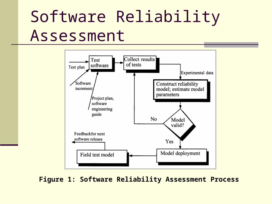
Figure 1: Software Reliability Assessment Process
Software Reliability Model Development Process
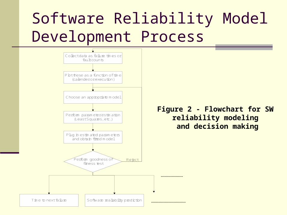
Collect data as failure times or fault counts
Plot these as a function of time (calender or execution)
Choose an appropriate model
Perform parameter estimation(Least Squares, etc.)
Plug in estimated parameters and obtain fitted model
Perform goodness of fitness test
Reject
Time to next failure Software realiability prediction
Figure 2 - Flowchart for SW reliability modeling
and decision making

Basic Definitons
Failures: A failure occurs when the user perceives that a software program ceases to deliver the expected service.
Faults: A fault is the cause of the failure or the internal error (e.g. an incorrect state). It is also referred as a “bug”.
Defects: When the distinction between fault and failure is not critical, “defect” can be used as a generic term to refer to either a fault (cause) or a failure (effect).
Errors: 1) A discrepancy between a computed, observed, or measured value or condition and the true, specified, or theoretically correct value or condition. 2) A human action that results in software containing a fault. (the term “mistake” is used instead to avoid the confusion)
Basic Definitons
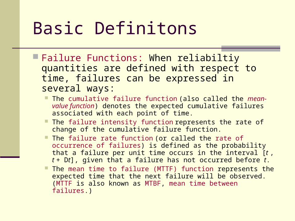
Failure Functions: When reliabiltiy quantities are defined with respect to time, failures can be expressed in several ways: The cumulative failure function (also called the mean-value
function) denotes the expected cumulative failures associated with each point of time.
The failure intensity function represents the rate of change of the cumulative failure function.
The failure rate function (or called the rate of occurrence of failures) is defined as the probability that a failure per unit time occurs in the interval [t , t + Dt], given that a failure has not occurred before t.
The mean time to failure (MTTF) function represents the expected time that the next failure will be observed. (MTTF is also known as MTBF, mean time between failures.)
Basic Definitons
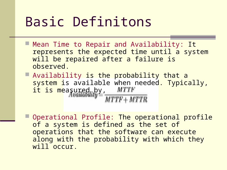
Mean Time to Repair and Availability: It represents the expected time until a system will be repaired after a failure is observed.
Availability is the probability that a system is available when needed. Typically, it is measured by,
Operational Profile: The operational profile of a system is defined as the set of operations that the software can execute along with the probability with which they will occur.

Hardware Reliability vs. Software ReliabilitySome of the important differences between software and hardware
reliability are: Failure does not occur if the software is not used. However in
hardware reliability, material deterioration can cause failure even when the system is not in use.
In software reliability, failures are caused by incorrect logic, incorrect statements, or incorrect input data. In hardware reliability, failures are caused by material deterioration, random failures, design errors, misuse, and environmental factors.
Software failures are rarely preceded by warnings while hardware failures are usually preceded by warnings.
Software essentially requires infinite testing, whereas hardware can usually be tested exhaustively.
Software does not wear out, and hardware does.

Classification of SW Reliability Models - 1 There are lots of different classification
schemas of SW Reliability Models. One of these classification schemas:
SW Reliability Models can be categorized into two types of models:
1. Deterministic Models
2. Probabilistic Models

Classification – Deterministic Models
Represent a quantitative approach to the measurement of computer software. It is used to study:
1. The elements of a program by counting the number of operators, operands and instructions.
2. The control flow of a program by counting the branches and tracing the execution path.
3. The data flow of a program by studying the data sharing and data passing.
Classification – Deterministic Models
There are two models in the deterministic type:
1. Halstead's software science model: to estimate the number of errors in the program,
2. McCabe's cyclomatic complexity model: to determine an upper bound on the number of tests in a program.
Classification – Probabilistic Models
Represent the failure occurrences and the fault removals as probabilistic events.
It is divided into different groups of models:
1. Error seeding 6. Execution path
2. Failure rate 7. Program structure
3. Bayesian and unified 8. Markov
4. Nonhomogeneous Poisson process
5. Input domain

Probabilistic Models – Error Seeding
1. Error Seeding Estimates the number of errors in a program by
using the capture-recapture sampling technique.
The capture-recapture sampling technique: Errors are divided into indigenous errors and
induced errors (seeded errors). The unknown number of indigenous errors is
estimated from the number of induced errors and the ratio of the two types of errors obtained from the debugging data.
Probabilistic Models – Failure Rate
3. Failure Rate It is used to study the functional forms of the
per-fault failure rate and program failure rate at the failure intervals.
Models included in this group are the
• Jelinski and Moranda De-Eutrophication
• Schick and Wolverton
Probabilistic Models – Reliability growth
4. Reliability Growth Measures and predicts the improvement of
reliability through the debugging process. A growth function is used to represent the
progress. Models included in this group are the
• Duane growth
• Weibull Growth

Probabilistic Models – Program Structure5. Program Structure Views a program as a reliability network. A node represents a module or a subroutine, and
the directed arc represents the program execution sequence among modules.
By estimating the reliability of each node, the reliability of transition between nodes, the transition probability of the network, and assuming independence of failure at each node, the reliability of the program can be solved as a reliability network problem.

Probabilistic Models – Program Structure Models included in this group are the
• Littlewood Markov structure
• Cheung's user-oriented Markov

Probabilistic Models – Input Domain
6. Input Domain Uses run (the execution of an input state) as
the index of reliability function. The reliability is defined as the number of
successful runs over the total number of runs.
Models included in this group are the
• Basic input-domain
• Input-domain based stochastic.
Probabilistic Models – Execution Path
7. Execution Path Estimates software reliability based on the
probability of executing a logic path of the program and the probability of an incorrect path.
This model is similar to the input domain model because each input state corresponds to an execution path.
The model forming this group is the• Shooman decomposition
Probabilistic Models – Execution Path
8. Nonhomogeneous Poisson Process Provides an analytical framework for describing the
software failure phenomenon during testing. The main issue in the NHPP model is to estimate
the mean value function of the cummulative number of failures experienced up to a certain time point.
Models included in this group are the
• Musa exponential
• Goel and Okumoto NHPP
Probabilistic Models – Markov
9. Markov Is a general way of representing the software failure
process. The number of remaining faults is modeled as a stochastic counting process.
If we assume that the failure rate of the program is proportional to the number of remaining faults, the two models are available: • linear death process: assumes that the remaining error
is nonincreasing
• linear birth-and-death process: allows faults to be introduced during debugging.
Probabilistic Models – Markov
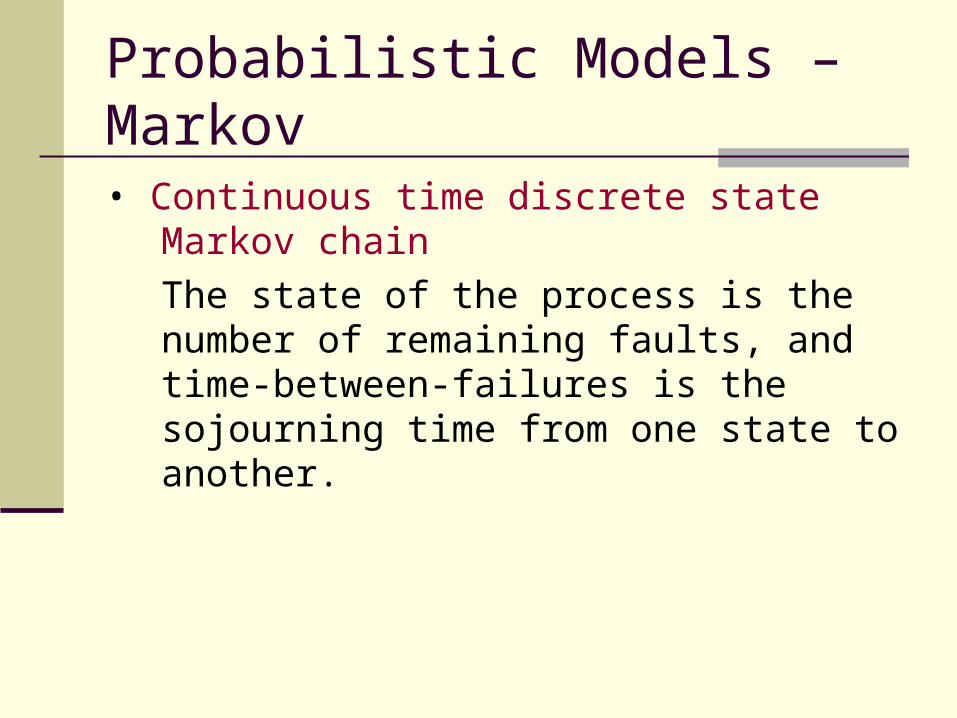
• Continuous time discrete state Markov chain
The state of the process is the number of remaining faults, and time-between-failures is the sojourning time from one state to another.
Probabilistic Models – Markov
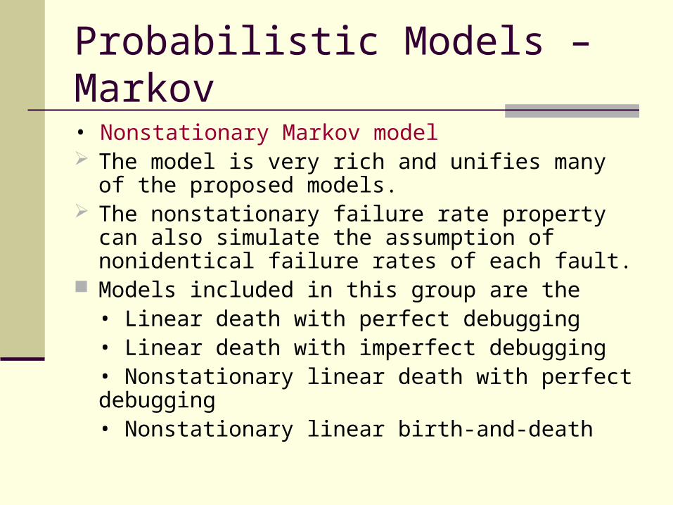
• Nonstationary Markov model The model is very rich and unifies many of the
proposed models. The nonstationary failure rate property can also
simulate the assumption of nonidentical failure rates of each fault.
Models included in this group are the• Linear death with perfect debugging• Linear death with imperfect debugging• Nonstationary linear death with perfect debugging• Nonstationary linear birth-and-death

Probabilistic Models – Bayesian and Unified
10. Bayesin and Unified Assume a prior distribution of the failure
rate. These models are used when the software
reliability engineer has a good feeling about the failure process, and the failure data are rare.
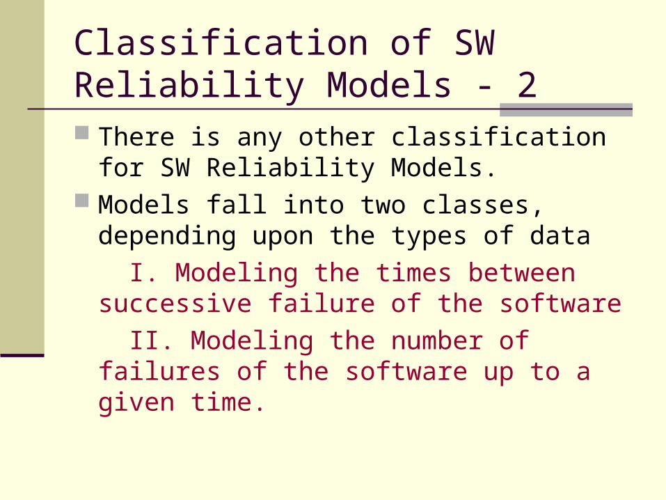
Classification of SW Reliability Models - 2 There is any other classification for SW
Reliability Models. Models fall into two classes, depending upon
the types of data
I. Modeling the times between successive failure of the software
II. Modeling the number of failures of the software up to a given time.

Classification of SW Reliability Models - 2 Time between failure models
Geometric Jelinski-Moranda Littlewood-Verrall Musa-Basic Musa-Okumoto

Classification of SW Reliability Models - 2 Failure Count models
Schneidewind Shick-Wolverton Yamada S-shaped
Geometric Model
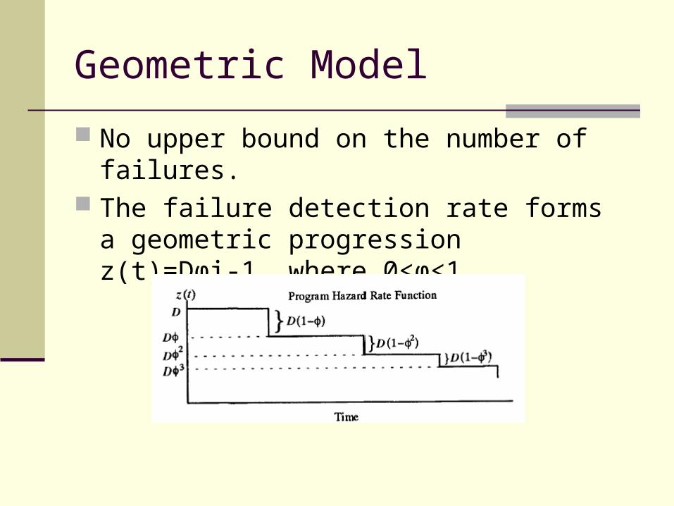
No upper bound on the number of failures. The failure detection rate forms a geometric
progression z(t)=Dφi-1 where 0<φ<1
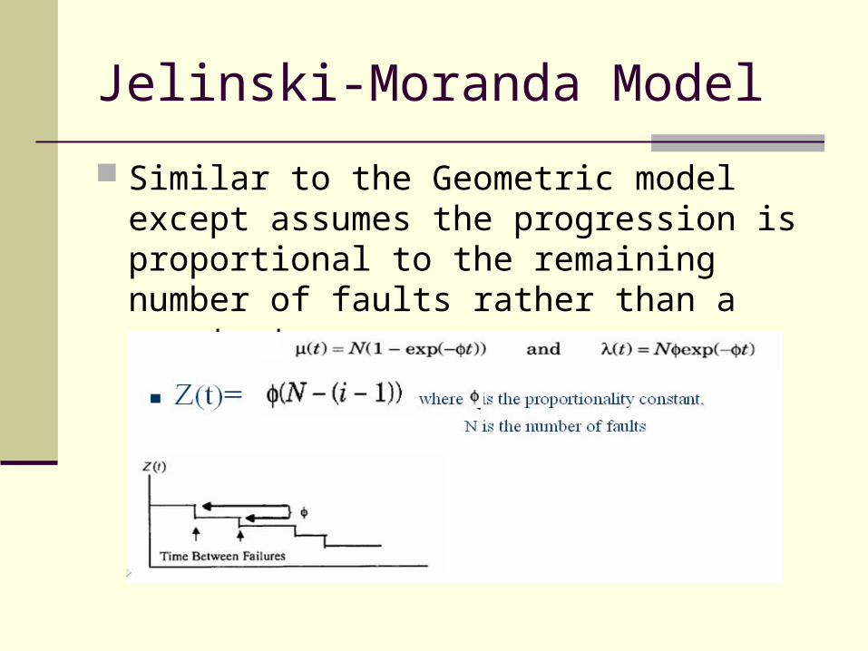
Jelinski-Moranda Model
Similar to the Geometric model except assumes the progression is proportional to the remaining number of faults rather than a constant.
Littlewood-Verrall Model
This model makes the assumption that fault correction is imperfect, therefore new faults will be generated as ones discovered are fixed.

Musa Basic Model
Uses execution time rather than calendar time.
0 is equal to the number of faults in the system and 1 is a fault reduction factor.

Musa-Okumoto Model
Differs from basic Musa in that it reflects the view that the earlier discovered failures have a greater impact on reducing the failure intensity function than those encountered later.
Schneidewind
Assumes that the current fault rate might be a better predictor of the future behaviour than the observed rate in the distant past
Three forms of the model that reflect the analyst’s view of the importance of the data as functions of time. Model 1: All the data points are of equal
importance Model 2: Ignore the fault counts completely from
the first through the s-1 time periods Model 3: Use the cumulative fault counts from the
intervals 1 to s-1 as the first data point.
Shick-Wolverton
Assumes the expected number of failures in any time interval is proportional to the fault content at the time of testing , and the time elapsed since the last failure.
Z(t|ti-1) = (N-i+1)β(t+ti-1) t Є [ti-1 , ti)
Where N is the number of faults
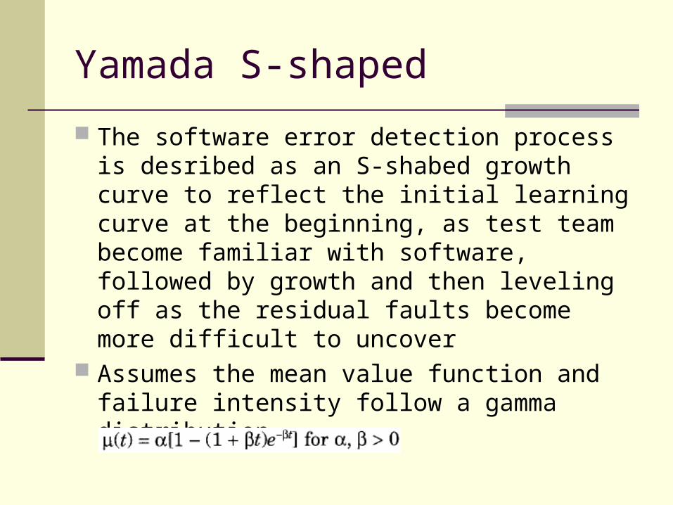
Yamada S-shaped
The software error detection process is desribed as an S-shabed growth curve to reflect the initial learning curve at the beginning, as test team become familiar with software, followed by growth and then leveling off as the residual faults become more difficult to uncover
Assumes the mean value function and failure intensity follow a gamma distribution
Conclusion
Software reliability is the probability that a system functions without failure for a specified time in a specified environment
Software Reliability models try to encourage the reliability level of the software.
There is no single model that can be used in all situations.
“There is no a silver-bullet!”

REFERENCES
Energy Citatitions Database http://www.osti.gov/energycitations/purl.cover.jsp;jsessionid=CE7D0E16AE9C5411F84656C31F73AE5E?purl=/6017897-Rc1ams/
Software Reliability Modeling Nozer D. Singpurwalla and Simon P. Wilson http://www.jstor.org/pss/1403763