PROCEEDINGS Open Access

Software tool for 3D extraction of germinal centersDavid N Olivieri1*, Merly Escalona1, Jose Faro2,3*

From 10th International Conference on Artificial Immune Systems (ICARIS)Cambridge, UK. 18-21 July 2011

Abstract

Background: Germinal Centers (GC) are short-lived micro-anatomical structures, within lymphoid organs, whereaffinity maturation is initiated. Theoretical modeling of the dynamics of the GC reaction including follicular CD4+

T helper and the recently described follicular regulatory CD4+ T cell populations, predicts that the intensity and lifespan of such reactions is driven by both types of T cells, yet controlled primarily by follicular regulatory CD4+

T cells. In order to calibrate GC models, it is necessary to properly analyze the kinetics of GC sizes. Presently, theestimation of spleen GC volumes relies upon confocal microscopy images from 20-30 slices spanning a depthof ~ 20 - 50 μm, whose GC areas are analyzed, slice-by-slice, for subsequent 3D reconstruction and quantification.The quantity of data to be analyzed from such images taken for kinetics experiments is usually prohibitively largeto extract semi-manually with existing software. As a result, the entire procedure is highly time-consuming, andinaccurate, thereby motivating the need for a new software tool that can automatically identify and calculate the3D spot volumes from GC multidimensional images.

Results: We have developed pyBioImage, an open source cross platform image analysis software application,written in python with C extensions that is specifically tailored to the needs of immunologic research involving 4Dimaging of GCs. The software provides 1) support for importing many multi-image formats, 2) basic imageprocessing and analysis, and 3) the ExtractGC module, that allows for automatic analysis and visualization ofextracted GC volumes from multidimensional confocal microscopy images. We present concrete examples ofdifferent microscopy image data sets of GC that have been used in experimental and theoretical studies of mousemodel GC dynamics.

Conclusions: The pyBioImage software framework seeks to be a general purpose image application forimmunological research based on 4D imaging. The ExtractGC module uses a novel clustering algorithm forautomatically extracting quantitative spatial information of a large number of GCs from a collection of confocalmicroscopy images. In addition, the software provides 3D visualization of the GCs reconstructed from the imagestacks. The application is available for public use at http://sourceforge.net/projects/pybioimage/.

BackgroundDuring the later phase of primary immune responses toprotein antigens, as well as in secondary immune responsesto the same antigen, the produced antibodies display higheraffinity for their antigen compared with the early phase ofthe response, a phenomenon known as affinity maturation[1]. The precise mechanisms responsible for this phenom-enon are the subject of current intense research, and are

known to take place in well-organized micro-anatomicalstructures, called germinal centers (GC), that develop tem-porarily within primary follicles of secondary lymphoidorgans during immune responses to protein antigens [2].The number of GCs and their average size increases

dramatically within the first week after immunizationand then start to decrease within days 10-14, so that bydays 21-24 very few of them remain, while those that dohave small sizes. GCs consist of a dominant populationof antigen-specific B cells and smaller populations of Tlymphocytes, follicular dendritic cells, and macrophages[3-5]. The antigen-specific B cells proliferate intensely,

* Correspondence: olivieri@ei.uvigo.es; jfaro@uvigo.es1School of Computer Engineering, University of Vigo, Ourense, 32004, Spain2Department of Biochemistry, Genetics and Immunology, University of Vigo,Vigo, 36310, SpainFull list of author information is available at the end of the article

Olivieri et al. BMC Bioinformatics 2013, 14(Suppl 6):S5http://www.biomedcentral.com/1471-2105/14/S6/S5

© 2012 Olivieri et al.; licensee BioMed Central Ltd. This is an open access article distributed under the terms of the Creative CommonsAttribution License (http://creativecommons.org/licenses/by/2.0), which permits unrestricted use, distribution, and reproduction inany medium, provided the original work is properly cited.

undergo somatic hypermutation in the variable region oftheir antibody molecules, and are subject to a poorlyunderstood affinity-based selection process [2,6].The long-held interest in GCs stems from being the

place where a Darwinian process, involving somatic hyper-mutation (SHM) and selection, acts on responding B cellsand their antibodies, thereby leading to memory B cellgeneration and to the phenomenon of affinity maturation.Because of the very high rate of SHM (10-4 to 10-3 perbase pair and cell division), a GC reaction with an exces-sively long duration may not only spoil previous affinityenhancing mutations, but also generate autoreactive andeven aberrant mutations leading to leukemia cells. Contra-rily, because of the random character of SHM, affinity-enhancing mutations appear only several days after theactivation of hypermutation, so that GC reactions withdurations too short will have an ineffectual selection. As aresult, it is not totally surprising that the time scale of GCreactions is regulated. The precise mechanisms that driveand control the dynamics of GCs are not presently knownand is the focus of intense research.Recently some of us [7] and others [8,9] have shown that

the dynamics of GCs is controlled by follicular regulatoryCD4+ T (TFreg) lymphocytes, a newly discovered distinctsubpopulation of Foxp3+CD4+ T cells that share with folli-cular CD4+ T helper cells the same responsiveness to thefollicular chemokine CXCL13. The impact of TFreg on thekinetics of GC sizes was made evident in studies involvingconfocal microscopy analysis of murine mesenteric lymphnodes at different times after immunization [7]. Our theo-retical modeling of the dynamics of the GC reaction,including TFreg cells, suggests that the intensity and lifespan of such a reaction is subject to two different control-ling processes: an initial process driven by TFreg cells, anda later one, detectable only when the first process is tooweak, controlled by follicular CD4+ T helper cell matura-tion (JF, manuscript in preparation). In order to properlycalibrate GC models with TFreg lymphocytes, comparisonsand fits to experimentally obtained GC sizes taken at dif-ferent time during the kinetics of entire process is funda-mental. A sufficiently accurate study, however, requires amore exhaustive analysis with the acquisition of moretime points during the immune response than previouslyaccomplished in experiments to date. Also, such an analy-sis would require accurate determination of all the GCvolumes obtained from these experiments.Presently, the estimation of GC volumes relies upon

sectioning either the spleen or lymph nodes in severaltissue samples of approximately ~ 20 - 50 μm thicknessand performing immunohistochemical staining. Subse-quently, confocal microscopy is used to acquire imagesfrom each section at different equally spaced planedepths, usually generating more than 20-30 thin slices.These image slices are then digitized and assembled into

Z-stacks, as shown in Figure 1. Finally, using a programsuch as ImageJ [10,11], the analysis of GC areas is per-formed semi-manually slice-to-slice, in the Z-stack, forsubsequent 3D reconstruction. Such a tedious and highlytime-consuming procedure provides a crude estimationof GC volumes. Moreover, the sheer quantity of data tobe analyzed from this large set of confocal microscopyimaging is so prohibitively large, that manual or semi-manual extraction is not tenable. Indeed, for understand-ing the order of magnitude of data produced, a typicalexperiment for study GC dynamics involves the analysisof on average ~100 GCs (5-10 slices per GC) per mouseand per time point (minimum 3-4 mice per time pointand 4-5 time points). As a result, there may be more than6000 individual GC slices to be analyzed in a singleexperiment.Available software A candidate software application for

the proposed task would provide automatic measurementsof all GC densities; that is, an accurate and automaticmeasure of the individual GC volumes, a count of the con-stituent cells, and subsequent visual confirmation of eachGC using a three dimensional isosurface reconstruction[12]. Perhaps the two most popular representative open-source software tools used for post-processing of micro-scopy images are ImageJ [10,11] (together with a newerdistribution branch, Fiji [13]) and OMERO [14-16]. Otheropen-source software tools for biological visualizationinclude Vaa3D (http://www.vaa3d.org), which is a crossplatform tool geared towards biological visualization of3D/4D/5D formats, and Icy (http://icy.bioimageanalysis.org), which is another powerful image analysis softwarethat provides a powerful environment for third partydevelopers together with visualization software. Severalcommercial software applications, such as Imaris andMetaMorph, are also widely used by the biology commu-nity for performing post-processing image analysis andvisualization tasks. While a complete listing or comparisonof all available software solutions are beyond the scope ofthis paper, these applications are certainly state-of the artand highly representative of other applications with theirparticular advantages/disadvantages. Also, in keeping withour design philosophy, we have focused more upon open-source analysis tools for comparing our software andalgorithms.In the case of OMERO, this is a large client/server appli-

cation, designed to provide centralized access of imagesfrom a disk server, and provides many types of analysis aswell as data annotation and workflow. While OMERO hasa large user base, and many analysis extensions, it pre-sently lacks the ability to automatically perform segmenta-tion of objects such as GCs in 3D (also referred to as 3Dspot volumes) and does not provide a 3D output thatallows for visual checking of the accuracy of the borders ofthe detected GCs. Moreover, there is no provision in their

Olivieri et al. BMC Bioinformatics 2013, 14(Suppl 6):S5http://www.biomedcentral.com/1471-2105/14/S6/S5

Page 2 of 12

roadmap for the addition of these difficult, yet importantfeatures [14].Fiji/ImageJ, is a multi- platform Java-based application

written for the desktop that uses the powerful ImageJimage analysis library for a microscopy specific applica-tion. It features extendible plug-in module support, script-ing in multiple languages, and supports a large collectionof image formats used the microscopy community. In anindependently developed branch, Fiji, provides many newpowerful analysis extensions; an example of which isimage registration techniques [17-19], for stitching multi-dimensional images from low-level autocorrelation of fea-tures. Nonetheless, it also does not contain the capabilityfor automatic segmentation of volumes with constituentcells, as envisioned in this work.In summary, with respect to segmenting and extracting

GC volumes, the microscopy software applications andalgorithms that we have evaluated either (a) lack sufficientinformation about the segmented dimensions, (b) underes-timate the number of objects segmented due to the diffi-culty of selecting the appropriate input parameters, (c)provide only gross estimates of areas/volumes, or (d) sim-ply do not provide the desired functionality for automati-cally obtaining GC volumes. As such, with respect toextracting GC volumes, no single software tool exists, toour knowledge, able to perform the proposed automatedtasks and that meets all requirements desired.While ImageJ and Fiji have a large user base and provide

the ability to write customized plug-ins in various pro-gramming languages, we decided from the onset to deviatefrom this standard development course in order todevelop our own microscopy infrastructure, written inpython and called pyBioImage. While motivated by sev-eral reasons, the principle advantage of this design choiceis to leverage the growing software base for scientific com-puting with powerful and efficient numerical and visual

libraries recently made available in the python community.Given the power of the python C-extension API, availablelibraries, and the ability for rapid and robust open softwaredevelopment, other microscopy software application haverecently emerged, albeit with slightly different scientificgoals, but based upon a similar python/C design philoso-phy. Two recent open source tools also written in pythonand C/C++, which have recently been reported in the lit-erature for microscopy applications, are IOCBioMicro-scope [20] (focused upon deconvolution of microscopyimages) and BioImageXD [21].

ImplementationOur software suite, pyBioImage, is a cross-platform bio-imaging application, written in Python and makes use oflow level C code exposed through the Python C-extensionAPI. The application supports multiple data formats andprovides visualization and analysis of standard multi-dimensional image data. For the work described in thispaper, we have developed a set of algorithms implementedeither in pure python or as python/C-extension modules,that form a core feature called ExtractGC, which is specifi-cally tailored for automatically extracting GC volume sta-tistics and visualization from a collection of 3D confocalfluorescent microscopy image stacks. These images arehighly magnified regions of tissue samples taken fromsecondary lymphoid organs. The set of such images fromtissue specimens may be used to reconstruct a 3D mosaic,consisting of several GCs, and thereby making it possiblevisualize a large section of the organ in question. Our ana-lysis software module ExtractGC, which is part of the moregeneral pyBioImage application, uses a pseudo-recursivesegmentation algorithm for performing simultaneous pixellevel clustering in all directions xyz of a complete imagestack. Our segmentation technique is based upon a generalsegmentation algorithm, often referred to as spot finding

Figure 1 Fluorescent confocal microscopy image of germinal centers. (a) Confocal microscopy image showing a germinal center (greenlabeled cells) together with the outer zone in a draining lymph node from a mouse at day 17 after immunization. (b) The image mosaic of alarger portion of the lymph node specimen formed from individual images of germinal centers. (c) A graphical representation of the 3D stackformed from the images slices togehter with a construction of the GC volumes.

Olivieri et al. BMC Bioinformatics 2013, 14(Suppl 6):S5http://www.biomedcentral.com/1471-2105/14/S6/S5

Page 3 of 12

algorithm in the context of fluorescent microscopy, firstdescribed and implemented by Goldberg and col. [22].In order to maintain the goal of cross-platform intero-

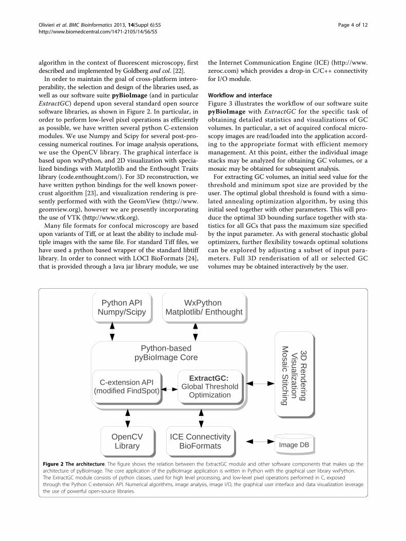
perability, the selection and design of the libraries used, aswell as our software suite pyBioImage (and in particularExtractGC) depend upon several standard open sourcesoftware libraries, as shown in Figure 2. In particular, inorder to perform low-level pixel operations as efficientlyas possible, we have written several python C-extensionmodules. We use Numpy and Scipy for several post-pro-cessing numerical routines. For image analysis operations,we use the OpenCV library. The graphical interface isbased upon wxPython, and 2D visualization with specia-lized bindings with Matplotlib and the Enthought Traitslibrary (code.enthought.com/). For 3D reconstruction, wehave written python bindings for the well known power-crust algorithm [23], and visualization rendering is pre-sently performed with with the GeomView (http://www.geomview.org), however we are presently incorporatingthe use of VTK (http://www.vtk.org).Many file formats for confocal microscopy are based

upon variants of Tiff, or at least the ability to include mul-tiple images with the same file. For standard Tiff files, wehave used a python based wrapper of the standard libtifflibrary. In order to connect with LOCI BioFormats [24],that is provided through a Java jar library module, we use

the Internet Communication Engine (ICE) (http://www.zeroc.com) which provides a drop-in C/C++ connectivityfor I/O module.

Workflow and interfaceFigure 3 illustrates the workflow of our software suitepyBioImage with ExtractGC for the specific task ofobtaining detailed statistics and visualizations of GCvolumes. In particular, a set of acquired confocal micro-scopy images are read/loaded into the application accord-ing to the appropriate format with efficient memorymanagement. At this point, either the individual imagestacks may be analyzed for obtaining GC volumes, or amosaic may be obtained for subsequent analysis.For extracting GC volumes, an initial seed value for the

threshold and minimum spot size are provided by theuser. The optimal global threshold is found with a simu-lated annealing optimization algorithm, by using thisinitial seed together with other parameters. This will pro-duce the optimal 3D bounding surface together with sta-tistics for all GCs that pass the maximum size specifiedby the input parameter. As with general stochastic globaloptimizers, further flexibility towards optimal solutionscan be explored by adjusting a subset of input para-meters. Full 3D renderisation of all or selected GCvolumes may be obtained interactively by the user.

Figure 2 The architecture. The figure shows the relation between the ExtractGC module and other software components that makes up thearchitecture of pyBioImage. The core application of the pyBioImage application is written in Python with the graphical user library wxPython.The ExtractGC module consists of python classes, used for high level processing, and low-level pixel operations performed in C, exposedthrough the Python C-extension API. Numerical algorithms, image analysis, image I/O, the graphical user interface and data visualization leveragethe use of powerful open-source libraries.

Olivieri et al. BMC Bioinformatics 2013, 14(Suppl 6):S5http://www.biomedcentral.com/1471-2105/14/S6/S5

Page 4 of 12

Segmentation algorithm for extracting germinal centervolumesBroadly speaking, segmentation algorithms decomposean image into distinct parts for recognizing objects ofinterest. These algorithms can be divided into threegroups: statistical feature-based, region-growing, andboundary methods [25,26]. For multidimensional images,feature based and boundary methods use image registra-tion algorithms [27] to associate image pixels of oneimage to those of another. There are many techniquesfor accomplishing this task, including pixel-wise compar-isons, cross-correlations, and scale invariant feature-based methods. These techniques have been extensivelystudied and applied to multi-dimensional medical andmicroscopy imaging for reconstructing volumes from dif-ferent z-stack slices. Region growing methods performsegmentation by low-level pixel assembly, subject tosome condition related to the pixels intensities of nearbyneighbors. For multidimensional microscopy images, theFindSpot algorithm described by I. Goldberg [22], hasbeen shown to be effective for constructing spot volumes,which are the bright/dark regions of interest, by recur-sively obtaining correspondence between neighboringpixels on the same and different image slices. By manu-ally providing threshold and geometric constraints, thealgorithm can efficiently encounter 3D continuous objectvolumes within and throughout the multidimensionalimage. Given the power of this method, our GC volumeextraction software uses the core part of this algorithmtogether with several practical software modifications aswell as additional algorithm details, described below.

Optimal global thresholdTwo fundamental parameters of the findspot algorithm (asdeveloped by Goldberg and col.) are the pixel threshold th,

which determines which pixels are allowed into a contigu-ous cluster, and the minimum cluster size smin (or spotsize), which provides a final cut-off on contiguous volumeregion. The threshold may be a global parameter or basedupon the mean pixel (or even more sophisticated statisti-cal-based methods, which for our purpose are not effec-tive). With fluorescent microscopy, the intensity is directlyproportional to the amount of B-cell membrane marker orreceptor molecules, which is relatively homogeneousthroughout the volume. Thus, it is sensible that a globalthreshold should be used since it will provide the mostaccurate indication of the amount of cells of a particulartype at a particular z-slice. Also, a proper segmentation ofthe GC areas on each slice will be sensitive to an optimalselection of the initial values of th and smin, where eachdepends upon the other.First, it is useful to understand the effect of the global

threshold th and smin parameters upon the final segmenta-tion of GC volumes, and in particular why this selection isnon-trivial. For segmenting the central part of a GC, asseen in Figure 4, slice 19, a particular threshold will per-form well; however for the image slices at the extremes (inthe z-plane), it becomes unclear which parameter valueslead to the best segmentation results. Indeed, if the thresh-old is too low, pixel clusters will be unnecessarily too large(possibly selecting the entire image). However, if thethreshold is too high, or optimized to the center of the GCwhere the fluorescent contrast is max, then on higher/lower z-stack slices, the GC borders, and hence GCvolumes, will be underestimated. With respect to theselection of the minimum spot size parameter, a smallminimal spot size will result in many pixel clusters thatare not germinal centers.For the specific case of segmenting GCs from multidi-

mensional images, we can use biological information to

Figure 3 The workflow. ExtractGC is based upon an easy to use, yet productive workflow for quickly obtaining GC size and volume statistics atthe lab bench. Given a set of confocal microscopy images, pyBioImage provides the option of direct visualization, image mosaic construction, ordirect analysis with the ExtractGC module. An automatic optimization algorithm iteratively selects the best input parameters for extracting GCvolumes. From the output of the analysis, the user may interact with the data via a 3D visualization.

Olivieri et al. BMC Bioinformatics 2013, 14(Suppl 6):S5http://www.biomedcentral.com/1471-2105/14/S6/S5

Page 5 of 12

guide the choice of an appropriate objective function. Inparticular, it is well known that by staining tissue sam-ples with flourochrome-tagged peanut agglutinin, GCswill be brightly labeled throughout the volume and con-sist of fluorescently marked B cells that are involved inthe immune response, while adjacent regions are charac-terized by a pronounced dark ring or halo. This darkouter ring zone is due to both follicular B cells not par-ticipating in the immune response (and, therefore, arenot antibody-flourochrome labeled) and to T and den-dritic cells of the adjacent T-cell zone, which are alsounlabeled.Given this nearly universal observed GC structure, an

ideal segmentation algorithm for GCs will include all pixelsup to and including the border adjacent to the dark halozone. Since the global threshold parameter of our algo-rithm directly controls this segmentation, our algorithmoptimizes this choice of threshold that segments the GCby the use of an iterative procedure, driven by a simulatedannealing algorithm that minimize the objective function,applied to all z-slices. This objective function seeks a mini-mum in the sum of pixel-tone histogram differences for allz-slices, between different values of the input parameters,while at the same time strongly penalizing solutions thatgive rise to segmented borders outside the GC region. Thealgorithm for optimizing the input parameters can be for-malized by referring to Figure 5 as follows. First, letθi(i = 1 · · ·m) represent the set of m input parameters tobe optimized. We denote the set of values of these para-meters at the iteration step t as λt = {θ t

i }. Next, we con-sider GC segmentation regions obtained from the findspotalgorithm. The segmentation region of the j-th GC on then-th image slice and at iteration step t is denoted by

γ nj (λt). Similarly, the segmentation region of the j-th GCregion on the n-th slice at iteration t’ is given by γ n

j (λt′).From this, we can obtain the fraction of the number ofpoints above the threshold Nf in the annular regionbetween γ n

j (λt) and γ nj (λt′) as compared to the total

number of pixels Nt in that annular region, as Nf /Nt.Moreover, for each of these regions, we can obtain thepixel-tone histogram, denoted H(γ n

j (λt)) ≡ Hnj (t). The

histograms for different segmented regionsγ nj , for a given

GC and a particular slice n corresponding to differentinput parameters λt are shown in Figure 6. As can be seenfrom this figure, the difference between histogramsdecreases as the segmented regions are closer. An optimalsolution, found from the optimal input parameters λ∗

twould produce a segmentation that wraps tightly aroundthe GC. Conversely, the value of the input parameters λt

should tend to maximize the individual areas of the seg-mented regions on all z-stack slices of each GC. Thus, theobjective function should penalize those values of theinput lt that eliminate areas at the extremes of the GCvolumes where the pixel intensities are at the limit ofthreshold. This tradeoff provides a convex objective func-tion for applying an optimization strategy.First, we use the Bhattacharyya histogram distance

metric

D(Ht ,Ht′) =

√√√√1 −∑

k,k′√Ht(k) · Ht′(k′)√∑

kHt(k) · ∑ k′Ht′(k′)

where Ht and Ht’, represent Hnj (λt) and Hn

j (λt′), and kand k’ represent the individual bins in each histogram,respectively.

Figure 4 GC borders obtained with the ExtractGC algorithm. Different z-stack slices of the GC from Figure 1a are shown together with theperformance of the segmentation algorithm. The green box represents the maximum bounding box, while the red curve is the convex hullenclosing all interior pixels above the desired intensity threshold for forming continuous clusters in 3D.

Olivieri et al. BMC Bioinformatics 2013, 14(Suppl 6):S5http://www.biomedcentral.com/1471-2105/14/S6/S5

Page 6 of 12

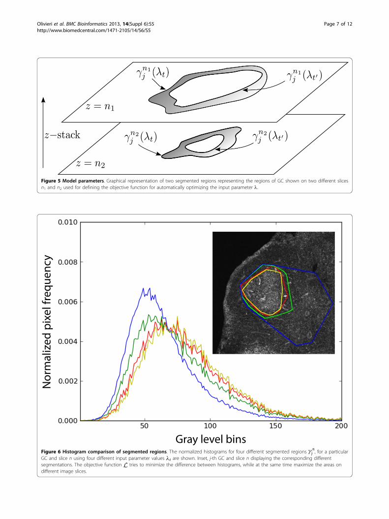
Figure 5 Model parameters. Graphical representation of two segmented regions representing the regions of GC shown on two different slicesn1 and n2 used for defining the objective function for automatically optimizing the input parameter l.

Nor

mal

ized

pix

el fr

eque

ncy

Gray level binsFigure 6 Histogram comparison of segmented regions. The normalized histograms for four different segmented regions γ n

j , for a particularGC and slice n using four different input parameter values λt are shown. Inset, j-th GC and slice n displaying the corresponding differentsegmentations. The objective function L tries to minimize the difference between histograms, while at the same time maximize the areas ondifferent image slices.

Olivieri et al. BMC Bioinformatics 2013, 14(Suppl 6):S5http://www.biomedcentral.com/1471-2105/14/S6/S5

Page 7 of 12

Now, let anj (λt) be the area of the segmentation regionγ nj (λt), that is, corresponding to the j-th GC at slice nusing input parameters l at iteration t, and let

Anj (λt ,λt′) =

|anj (λt) + anj (λt′)| − |anj (λt) − anj (λt′)||anj (λt) + anj (λt′)|

which is a symmetric function, since Anj (λt ,λt′) = An

j (λt′ ,λt).Then, we can define the objective function Lj for the j-thGC as follows:

Lj(λt,λt′) =

∑n exp[α D(Hn

j (λt),Hnj (λt′))]

ε + β∑

nAnj (λt,λt′)

where Î is a small nonzero constant that we insert toprevent division by zero error, while a and b are arbitraryconstants (we have used a ~ 0.001 and b = 1.0) that couldbe useful for controlling the strength of either the histo-gram difference or the sum over areas, respectively. Withthis function, the optimization is then with respect to theinput parameters λt = {θ t

i }, that is, ∂Lj/∂θi = 0. Notice thatif the areas anj (λt)and anj (λt′) on each slice n for each seg-mentation region j are very different —either becauseanj (λt) is much larger than anj (λt′) (or vice-versa) orbecause, suddenly, aj(λt) = 0 (oraj(λt′) = 0) due to thedisappearance of the contour at slice n—, thenLj(λt,λt′)and Lj(λt,λt′) grows to very large values, therebypenalizing Lj. Conversely, if a

nj (λt) = anj (λt′) (or are very

similar) then Anj (λt ,λt′) → 1.

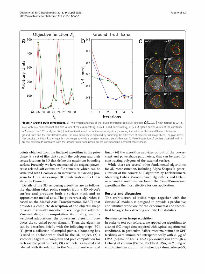
In general, the function Lj(λt,λt′) is a nonlinear multi-dimensional function with many local minimima, manyof which are not ideal solutions. In order to understandthe behavior of Lj as a function of λt and λt′, Figure 7(a)shows two hyperplane cuts with smin for different valuesof the threshold th. For constructing this plot, we choseconsecutive values of the threshold, with t′h = th + 1 (redcurve), and t′h = th + 2 (green curve). As can be seen, inboth planes, the function experiences a dramatic globalminimum for the optimal solution.From this objective function, we use a simulated

annealing algorithm that efficiently samples the space ofall possible λt in order to find the optimal set of inputparameters,λ∗, given by:

λ∗ = argminλt

Lj(λt,λt′)

In order to show how robuts our optimization algorithmis with respect to the choice of initial input parameters,Figure 7(b) shows the difference in accumulated area(which is related to the GC volume) between the calcu-lated and ground truth value for several iterations of thealgorithm for three separate initial values of l. In thesestudies, the ground truth determination was obtained frommanual inspection by an expert. Figure Figure 7(c) shows

a comparison, superposed on a particular Germinal Centerimage, between borders obtained with optimal parametersolution, l*, using our algorithm and the ground truthborder obtained by manual determination.Since the original findspot algorithm finds all contigu-

ous clusters of pixels throughout a volume, connectedregions can be filled with holes. By using a convex hullalgorithm, or more sophisticated computational geome-try algorithms based upon alpha shapes, we can representand visualize the 3-dimensional GC volumes with theouter bounding surface. Nearby artifacts due to outlierspoints may be present, distorting the volume estimate,and should be corrected. We eliminate outliers by a sim-ple heuristic algorithm that determines the full distancematrix between all points on the contour and determineswhether the distance between each point and all others isgreater than 2 × s value of all other inter point distances(where s is the standard deviation). Conversely, we canfind the geometric center and determine whether a pointis 2 × s from that center.Optimal stitching Our software pyBioImage also

contains a module for automatic stitching of multi-dimensional images, similar to that found in ImageJ.Side-by-side z-stack images of draining lymph nodeswere acquired to allow 3D reconstructions of largerorgan areas. Due to the large amount of image stacks, wedeveloped our own software algorithms that used infor-mation from the microscope position and accelerated thetask of forming large image mosaics, referred to as imagestitching, from adjacent z-stacks acquisitions.For matching adjacent image stacks, our algorithm uses

a fast implementation of the Fourier phase correlationtechnique for achieving image registration at the bordersof adjacent (and overlapping) images. For blending adja-cent images, we use a nonlinear pyramid scheme togetherwith pixel intensity scaling for matching potential differ-ences in acquisition exposures. The implementation of ouralgorithm is available in our cross-platform pyBioImagepackage, available at the public repository (sourceforge.net/projects/pybioimage/). Information about the installa-tion, documentation, and other software modules (whosedescription is beyond the scope of this paper), can also befound in the package distribution.3D reconstructionAnother capability of the ExtractGC module is the abilityto accurately visualize the GC volumes in 3D. The recon-struction of the set of borders pixels obtained from eachz-stack slice is used for constructing an isosurface with acomputational geometry algorithm, called Powercrust,described by Amenta, Choi and Kolluri [28,29]. We haveprovided a full set of python bindings to the original open-source C-language implementation of these authors inorder to easily expose the core algorithm to our applica-tion, pyBioImage. The output of powercrust, with the

Olivieri et al. BMC Bioinformatics 2013, 14(Suppl 6):S5http://www.biomedcentral.com/1471-2105/14/S6/S5

Page 8 of 12

points obtained from the findSpot algorithm in the priorphase, is a set of files that specify the polygons and theirvertex locations in 3D that define the maximum boundingsurface. Presently, we have maintained the original power-crust related .off extension file structure which can bevisualized with Geomview, an interactive 3D viewing pro-gram for Unix. An example 3D renderization of a GC isshown in Figure 8.Details of the 3D rendering algorithm are as follows:

the algorithm takes point samples from a 3D object’ssurface and produces both a surface mesh and anapproximate medial axis. The powercrust algorithm isbased on the Medial Axis Transformation (MAT) thatprovides a complete description of the object’s shapethrough maximally inscribed discs. Together with theVoronoi diagram computation its duality, and itsweighted adaptations, the powercrust algorithm pro-duces the so-called power diagram. Then, the algorithmcan be described briefly with the following steps [30]:(1) given a collection of sampled points, a bounding boxis used to enclose what shall be the 3D object, (2) aVoronoi Diagram is computed and pole computation foreach sample point is made, (3) each pole is analyzed andlabeled with its relation to the Voronoi surfaces, and

finally (4) the algorithm provides output of the power-crust and powershape parameters, that can be used forconstructing polygons of the external surface.While there are several other fundamental algorithms

for 3D reconstruction, including Alpha Shapes (a gener-alization of the convex hull algorithm by Edelsbrunner),Marching Cubes, Voronoi-based algorithms, and Delau-nay-based algorithms, we found the Crust/Powercrustalgorithms the most effective for our application.

Results and discussionThe architecture of pyBioImage, together with theExtractGC module, is designed to provide a productiveand intuitive workflow for the experimental and theore-tical biologist for extracting accurate GC statistics.

Germinal center image acquisitionIn order to test our software, we applied our algorithms toa set of GC image data acquired with typical experimentalconditions. In particular, Balb/c mice maintained in SPFfacilities were immunized intraperitoneally with 20 μg ofOVA (Sigma, St Louis, USA) previously run through aDetoxyGel column (Pierce, Rockford, USA) in 2.0 mg ofendotoxin-free aluminum hydroxide (alum, Alu-gel-S,

Objective function Lj Ground Truth Error500

400

300

200

100

0.8

0.6

0.7

0.5

0.4

0.3

64 66 68 70 72 0 1 2 3 474 76 78 80 5

Arb

itrar

y U

nits

A

[mm

2 ]

Iterationsth

a b c

Figure 7 Ground truth comparisons. (a) Two hyperplane cuts of the multidimensional objective function Lj(λt,λt′), with respect to l= (th,

smin), with smin held constant and two values of the arguments, t′h = th + 1 (red curve) and t′h = th + 2 (green curve); values of the constants

in Lj were a = 0.001 and b = 1.0. (b) Various iterations of the optimization algorithm, showing the values of the area difference betweenground truth and the calculated borders. The area difference is obtained by summing the difference of areas for all image slices. The plot showsthat despite the initial l, the algorithm converges towards a constant non-zero area difference. (c) Visual inspection of borders obtained with anoptimal solution l* compared with the ground truth, superposed on the corresponding germinal center image.

Olivieri et al. BMC Bioinformatics 2013, 14(Suppl 6):S5http://www.biomedcentral.com/1471-2105/14/S6/S5

Page 9 of 12

Serva, Heidelberg, Germany). Seventeen days after immu-nization the draining lymph nodes were excised and fixedwith PFA (Sigma). 50 μm vibratome sections from fixedtissue were stained with the following primary antibodies:rabbit anti-CD3 (Abcam), rat anti-IgM-TxRd (Southern-Biotech, Birmingham, USA), and PNA-FITC (Vector, Bur-lingam, USA). Anti-rabbit immunoglobulin-alexa647(Invitrogen, Carlsbad, USA) was used as secondaryantibody.Once the regions of interest were located, 35 images

were acquired at 1.43μm z-steps, using a LSM710 confo-cal microscope (Zeiss, Jena, Germany) equipped with a20 × (0,80 NA, Zeiss) objective. Several images wereacquired across a relatively large section of the specimen,such that each image contained at least one GC, and theset of all images formed a mosaic (with an irregularlyordered tiling).

EvaluationFrom the data, prepared as described above, we analyzedfour independent data sets that represent magnifiedregions of small sections of lymph nodes. For each speci-men, 5 GCs were imaged independently, with a slightoverlap of the nearby image, so that a mosaic could beformed. The images consisted of 4-color channels, were512 × 512, and contained an average of 30 z-stack slices.We used our algorithm to automatically collect GC statis-tics by loading all the images in the directory and provid-ing initial input parameter guesses for the pixel intensitythreshold and the minimum spot size: l = (th, smin).Results of extracting GCs for different datasets are shownin Figure 4, showing the contour encountered of the GCregion at different z-stack slices.The algorithms described are efficient, requiring no

special hardware, and can run on any modern computersystem. In order to appreciate the typical running times,we ran the algorithm on a standard laboratory computer(Intel Pentium D CPU 2.80GHz, with 2G Memory), andexecution times to process multi-dimensional imageswith sizes 512 × 512 × 35 never exceeded from 1.2 s and

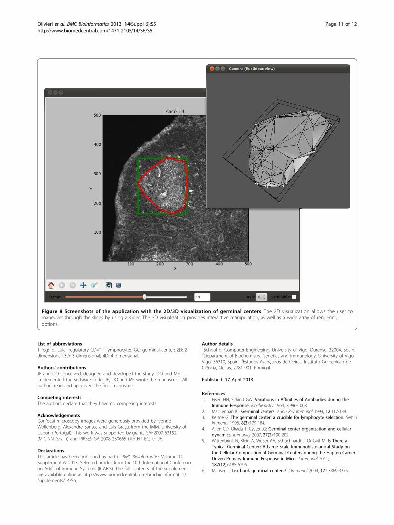
the execution time for the optimization step was alwaysbelow 0.5 s for different image sizes.Figure 9 illustrates the visualization features of pyBio-

Image/ExtractGC. The 2D window, allows the user tomaneuver through the image stacks slice by slice, withthe segmented contour superposed on the image. A 3Dvisualization allows the user to interactively manipulatethe GC volume from all angles, and provides a moreaccurate calculation of the GC volume.

ConclusionsOur application, pyBioImage with the ExtractGC mod-ule provides fully automatic and accurate estimates ofGC volumes from an arbitrarily large collection of mul-tidimensional images. The framework pyBioImageleverages the relatively recent availability of high qualityscientific software based upon python for rapid develop-ment of complex image and computation. As such, ourapplication is positioned to tackle several problemsdescribed in this paper not provided by standard open-source solutions, such as Fiji/ImageJ. The ExtractGCmodule is a relevant bioinformatics tool that should beof interest to scientists working with confocal and 2-photon microscopy imaging and has also served to be aproof of concept module for integrating specific applica-tions within our general software framework. Given theusefulness of the ExtractGC module, we are presentlyplanning to also release a version of the algorithm forboth the ImageJ as well as OMERO projects.

Availability and requirementsProject name: e.g. pyBioImage packageProject home page: http://sourceforge.net/projects/

pybioimage/Operating system(s): Platform independentProgramming language: phyton, COther requirements:License: GNU GPLAny restrictions to use by non-academics: license

needed

Figure 8 Examples of borders extracted for different germinal centers. ExtractGC analysis on five images of different germinal centers takenfrom the same specimen shown in the mosaic of Figure 1b. The images show the border (red curves) at slices in the center of each germinalcenter.

Olivieri et al. BMC Bioinformatics 2013, 14(Suppl 6):S5http://www.biomedcentral.com/1471-2105/14/S6/S5

Page 10 of 12

List of abbreviationsTFreg: follicular regulatory CD4+ T lymphocytes; GC: germinal center; 2D: 2-dimensional; 3D: 3-dimensional; 4D: 4-dimensional.

Authors’ contributionsJF and DO conceived, designed and developed the study, DO and MEimplemented the software code, JF, DO and ME wrote the manuscript. Allauthors read and approved the final manuscript.

Competing interestsThe authors declare that they have no competing interests.

AcknowledgementsConfocal microscopy images were generously provided by IvonneWollenberg, Alexandre Santos and Luis Graça, from the IMM, University ofLisbon (Portugal). This work was supported by grants SAF2007-63152(MICINN, Spain) and PIRSES-GA-2008-230665 (7th FP, EC) to JF.

DeclarationsThis article has been published as part of BMC Bioinformatics Volume 14Supplement 6, 2013: Selected articles from the 10th International Conferenceon Artificial Immune Systems (ICARIS). The full contents of the supplementare available online at http://www.biomedcentral.com/bmcbioinformatics/supplements/14/S6.

Author details1School of Computer Engineering, University of Vigo, Ourense, 32004, Spain.2Department of Biochemistry, Genetics and Immunology, University of Vigo,Vigo, 36310, Spain. 3Estudos Avançados de Oeiras, Instituto Gulbenkian deCiência, Oeiras, 2781-901, Portugal.

Published: 17 April 2013

References1. Eisen HN, Siskind GW: Variations in Affinities of Antibodies during the

Immune Response. Biochemistry 1964, 3:996-1008.2. MacLennan IC: Germinal centers. Annu Rev Immunol 1994, 12:117-139.3. Kelsoe G: The germinal center: a crucible for lymphocyte selection. Semin

Immunol 1996, 8(3):179-184.4. Allen CD, Okada T, Cyster JG: Germinal-center organization and cellular

dynamics. Immunity 2007, 27(2):190-202.5. Wittenbrink N, Klein A, Weiser AA, Schuchhardt J, Or-Guil M: Is There a

Typical Germinal Center? A Large-Scale Immunohistological Study onthe Cellular Composition of Germinal Centers during the Hapten-Carrier-Driven Primary Immune Response in Mice. J Immunol 2011,187(12):6185-6196.

6. Manser T: Textbook germinal centers? J Immunol 2004, 172:3369-3375.

Figure 9 Screenshots of the application with the 2D/3D visualization of germinal centers. The 2D visualization allows the user tomaneuver through the slices by using a slider. The 3D visualization provides interactive manipulation, as well as a wide array of renderingoptions.

Olivieri et al. BMC Bioinformatics 2013, 14(Suppl 6):S5http://www.biomedcentral.com/1471-2105/14/S6/S5

Page 11 of 12

7. Wollenberg I, Agua-Doce A, Hernandez A, Almeida C, Oliveira VG, Faro J,Graca L: Regulation of the germinal center reaction by Foxp3+ follicularregulatory T cells. J Immunol 2011, 187(9):4553-60.

8. Chung Y, Tanaka S, Chu F, Nurieva RI, Martinez GJ, Rawal S, Wang YH,Lim H, Reynolds JM, Zhou XH, Fan HM, Liu ZM, Neelapu SS, Dong C:Follicular regulatory T cells expressing Foxp3 and Bcl-6 suppressgerminal center reactions. Nat Med 2011, 17(8):983-8, [Doi: 10.1038/nm.2426.].

9. Linterman MA, Pierson W, Lee SK, Kallies A, Kawamoto S, Rayner TF,Srivastava M, Divekar DP, Beaton L, Hogan JJ, Fagarasan S, Liston A,Smith KG, Vinuesa CG: Foxp3+ follicular regulatory T cells control thegerminal center response. Nat Med 2011, 17(8):975-82, [Doi: 10.1038/nm.2425.].

10. Saalfeld S, Cardona A, Hartenstein V, Tomancak P: As rigid as possiblemosaicking and serial section registration of larte ssTEM datasets.Bioinformatics 2010, 26(12):i57-i63.

11. Cardona A, Saalfeld S, Preibisch S, Schmid B, Cheng A, Pulokas J,Tomancak P, Hartenstein V: An integrated micro- and MacroarchitecturalAnalysis of the Drosophila Brain by computer-Assisted serial sectionElectron Microscopy. PLoS Biol 2010, 8(10):e1000502.

12. Ourselin S, Roche A, Subsol G, Pnnec X, Ayache N: Reconstructing a 3dstructure from serial histological sections. Image and Vision Computing2001, 19:25-31.

13. Walter T, Shattuck DW, Baldock R, Bastin ME, Carpenter AE, Duce S,Ellenberg J, Fraser A, Hamilton N, Pieper S, Ragan MA, Schneider JE,Tomancak P, Heriche JK: Visualization of image data from cells toorganisms. Nat Methods 2010, 7(3 Suppl):S26-S41.

14. Swedlow J, Goldberg I, Eliceiri K, the OME Consortium: BioimageInformatics for Experimental Biology. Annu Rev Biophys 2009, 38:327-346.

15. Preibisch S, Saalfeld S, Tomancak P: Globally optimal stitching of tiled 3Dmicroscopic image acquisitions. Bioinformatics 2009, 25(11):1463-1465.

16. I Arganda-Carreras I, Sorzano C, Marabini R, Carazo J, Ortiz de Solorzano C,Kybic J: Consistent and Elastic Registration of Histologic sections usingvector spline regularization. Lecture Notes in Computer Science, Springer,CVAMIA 2006, 4241:85-95.

17. Zitová B, Flusser J: Image registration methods: a survey. Image and VisionComputing 2003, 21(11):977-1000 [http://www.sciencedirect.com/science/article/pii/S0262885603001379].

18. Bagci U, Bai L: Registration of standardized histological images in featurespace. Proceedings of SPIE, Volume 6914 Spie; 2009, 69142V-69142V-9 [http://arxiv.org/abs/0907.3209].

19. McInerney I, Terzopoulus T: Deformable Model sin Medical ImageAnalysis: A Survey. Medical Image Analysis 1996, 1(2):91-108.

20. Laasmaa M, Vendelin M, Peterson P: Application of regularizedRichardson-Lucy algorithm for deconvolution of confocal microscopyimages. J Microsc 2011, 243(2):124-140.

21. Kankaanpää P, Pahajoki K, Marjomäki V, Heino J, White D: BioImageXD -New Open Source Free Software for the Processing, Analysis andVisualization of Multidimensional Microscopic Images. Microscopy Today2006, 14(3):12-16.

22. Schiffmann D, Dikovskaya D, Appleton P, Newton I, Creager D, Allan C,Nathke I, Goldberg I: Open Microscopy Environment and FindSpots:integrating image informatics with quantitative multidimensional imageanalysis. BioTechniques 2006, 41:199-207.

23. Amenta N, Choi S, Kolluri R: The power crust, unions of balls, and themedial axis transform. Computational Geometry: Theory and Applications2001, 19(2-3):127-153.

24. Linkertm M, Rueden C, Allan C, Burel J, Moore W, Patterson A, Loranger B,Moore J, Neves C, Macdonald D, Tarkowska A, Sticco C, Hill E, Rossner M,Eliceiri K, Swedlow J: Metadata matters: access to image data in the realworld. J Cell Biol 2010, 189(5):777-782.

25. Shapiro LG, Stockman GC: Computer vision Upper Saddle River, NJ: PrenticeHall; 2001.

26. Szeliski R: Computer Vision: Algorithms and Applications Berlin, Germany:Springer; 2011.

27. Bagci U, Chen X, Udupa J: Hierarchical Scale-Based MultiobjectRecognition of 3-D Anatomical Structures. IEEE Trans Med Imaging 2012,31(3):777-789.

28. Amenta N, Bern M, Eppstein D: The Crust and the Beta-Skeleton:Combinatorial Curve Reconstruction. Graphical Models and ImageProcessing 1998, 60:125-135.

29. Amenta N, Choi S, Kolluri R: The power crust. Proceedings of the sixth ACMsymposium on Solid modeling and applications SMA ‘01, New York, NY, USA:ACM; 2001, 249-266 [http://doi.acm.org/10.1145/376957.376986].

30. Amenta N, Bern M: Surface Reconstruction by Voronoi Filtering. Discreteand Computational Geometry 1999, 22:481-504.

doi:10.1186/1471-2105-14-S6-S5Cite this article as: Olivieri et al.: Software tool for 3D extraction ofgerminal centers. BMC Bioinformatics 2013 14(Suppl 6):S5.

Submit your next manuscript to BioMed Centraland take full advantage of:

• Convenient online submission

• Thorough peer review

• No space constraints or color figure charges

• Immediate publication on acceptance

• Inclusion in PubMed, CAS, Scopus and Google Scholar

• Research which is freely available for redistribution

Submit your manuscript at www.biomedcentral.com/submit

Olivieri et al. BMC Bioinformatics 2013, 14(Suppl 6):S5http://www.biomedcentral.com/1471-2105/14/S6/S5

Page 12 of 12