AAllmmaa MMaatteerr SSttuuddiioorruumm –– UUnniivveerrssiittàà ddii BBoollooggnnaa

DOTTORATO DI RICERCA IN

INGEGNERIA CIVILE, AMBIENTALE E DEI MATERIALI

Ciclo XXVII

Settore Concorsuale di afferenza: 08/A2 Settore Scientifico disciplinare: ING-IND/28

SOIL-STRUCTURE INTERACTION DURING TUNNELLING IN URBAN

AREA: OBSERVATIONS AND 3D NUMERICAL MODELLING

Presentata da: Ing. VALENTINA FARGNOLI

Coordinatore Dottorato Relatore

Prof. Ing. Alberto LAMBERTI

Prof. Ing. Daniela BOLDINI

Correlatore

Prof. Ing. Angelo AMOROSI

Esame finale anno 2015

I

Abstract

This work illustrates a soil-tunnel-structure interaction study performed by an

integrated, geotechnical and structural, approach based on 3D finite-element analyses

and validated against experimental observations. The study aims at analysing the

response of reinforced concrete framed buildings on discrete foundations in interaction

with metro-lines. It refers to the case of the twin tunnels of the Milan (Italy) metro-line

5, recently built in coarse-grained materials using EPB machines, for which subsidence

measurements collected along ground and building sections during tunnelling were

available. Settlements measured under free-field conditions are firstly back-interpreted

using Gaussian empirical predictions. Then, the in situ measurements’ analysis is

extended to include the evolving response of a 9-storey reinforced concrete building

while being undercrossed by the metro-line. In the finite-element study, the soil

mechanical behaviour is described using an advanced constitutive model. This latter,

when combined with a proper simulation of the excavation process, proves to

realistically reproduce the subsidence profiles under free-field conditions and to capture

the interaction phenomena occurring between the twin tunnels during the excavation.

Furthermore, when the numerical model is extended to include the building,

schematised in a detailed manner, the results are in good agreement with the monitoring

data for different stages of the twin-tunnelling. Thus, they indirectly confirm the

satisfactory performance of the adopted numerical approach which also allows a direct

evaluation of the structural response as an outcome of the analysis. Further analyses are

also carried out modelling the building with different levels of detail. The results

highlight that, in this case, the simplified approach based on the equivalent plate

schematisation is inadequate to capture the real tunnelling-induced displacement field.

II

The overall behaviour of the system proves to be mainly influenced by the buried

portion of the building which plays an essential role in the interaction mechanism, due

to its high stiffness.

III

Sommario

Questo lavoro illustra uno studio di interazione terreno-galleria-struttura messo a punto

attraverso un approccio accoppiato, geotecnico e strutturale, basato su analisi

tridimensionali agli elementi finiti e validato mediante il confronto con osservazioni

sperimentali. Il principale obiettivo dello studio è l’analisi della risposta di edifici in

cemento armato su fondazioni discrete in interazione con linee metropolitane. Questo

studio si riferisce al caso delle due gallerie della linea 5 della metropolitana di Milano

(Italia), costruita di recente in terreni a grana grossa mediante macchine di tipo EPB, per

cui sono disponibili misure della subsidenza rilevate durante lo scavo, sia lungo sezioni

sul terreno sia in corrispondenza di edifici situati lungo la tratta. I cedimenti misurati in

condizioni di campo libero vengono prima interpretati mediante le classiche previsioni

empiriche di tipo gaussiano. L’analisi delle misure in sito viene successivamente estesa

ad analizzare la risposta di un edificio a nove piani in cemento armato sotto attraversato

dalla linea metropolitana, che evolve durante lo scavo. Nello studio agli elementi finiti,

la risposta meccanica del terreno è descritta mediante un modello costitutivo avanzato

che, se associato ad una appropriata simulazione del processo di scavo, è in grado di

riprodurre in modo realistico i profili di subsidenza di campo libero, nonché di cogliere

la mutua interazione tra le due gallerie durante la costruzione della linea metropolitana.

I risultati della simulazione condotta includendo nel modello numerico l’edificio

schematizzato in dettaglio sono in buon accordo con i dati di monitoraggio per differenti

fasi dello scavo. Ciò, dunque, conferma in modo indiretto la soddisfacente prestazione

dell’approccio numerico adottato, consentendo, inoltre, una valutazione diretta della

risposta strutturale come risultato dell’analisi. Ulteriori analisi numeriche eseguite con

modelli semplificati dell’edificio mettono in luce che, in questo caso, l’approccio basato

sul metodo della piastra equivalente è inadeguato a cogliere il reale campo di

IV

spostamenti generato dallo scavo. La risposta globale del sistema, inoltre, risulta

principalmente influenzata dalla porzione interrata dell’edificio che, data la sua elevata

rigidezza, ha un ruolo essenziale nel meccanismo di interazione.

1

1. Introduction

1.1 Purpose of the study

The construction of new metro-lines in urban areas often requires tunnel excavation to

be carried out in close proximity to residential buildings, cultural heritage monuments

and underground services. The ability to correctly predict the tunnelling-induced

settlements represents a key aspect to properly estimate potential damages on

pre-existing structures and to design protective measures, when needed. It is widely

recognised that the simplified approach for damage evaluation based on free-field

subsidence profiles, thus disregarding the influence of the structure stiffness and weight,

often leads to rather conservative solutions in terms of estimated differential settlements

and, consequently, of damage intensity.

In the last few years two-dimensional (2D) approaches which incorporate the structure

in the finite element analyses have been developed to overcome such limitations.

However, in several cases, a detailed investigation of the soil-tunnel-structure

interaction can only be performed by 3D numerical computations, which allow to

account for any construction scheme, including the case of twin tunnels, and for any

kind of surface structure and its relative position with respect to the tunnel axis.

Finite element simulations were mainly performed in the past with reference to masonry

surface structures affected by tunnelling. Conversely, this class of interaction studies

were more rarely carried out focusing on framed buildings, although being a structural

typology widely diffuse in urban areas.

The reliability of the numerical approaches is strongly affected by different factors, such

as the constitutive hypotheses for the soil, the correct simulation of the tunnel

excavation sequence and the detail of the structural modelling.

2

This work proposes a coupled, geotechnical and structural, 3D finite element approach,

performed by the code Plaxis 3D, aimed at investigating the soil-structure interaction

during tunnelling, with specific reference to reinforced concrete framed buildings. It

demonstrates the importance of a proper description of the soil mechanical behaviour,

associated to a correct schematisation of the tunnel construction and to an appropriate

structural modelling, to realistically simulate the response of the overall system to

tunnelling.

The ability of the proposed procedure to effectively capture the soil-tunnel-structure

interaction mechanism is validated against the available geotechnical and structural

monitoring measurements from a real case-history, i.e. the recent construction of the

two tunnels of the new Milan (Italy) metro-line 5 which, along its route, diagonally

underpasses a multi-storey reinforced concrete framed structure dating back to the end

of the 1950s.

1.2 Layout of the thesis

Chapter 2 presents a literature review on ground movements due to tunnel excavation

with reference to free-field conditions and in presence of surface structures. The

attention is given to closed-form empirical solutions for the prediction of

tunnelling-induced subsidence as well as to 2D and 3D numerical approaches which

allow a more accurate investigation of the soil-structure interaction. The methodology

generally employed to assess the damage potentially caused by tunnel construction to

surface buildings is also introduced and discussed.

Chapter 3 is focused on the case-history of the new metro-line 5 of Milan, excavated in

coarse-grained soils partially below the water table by two earth pressure balance (EPB)

machines that guaranteed low values of the surface volume loss. Settlement monitoring

data collected under free-field conditions during and after the excavation of the twin

3

tunnels of the line are examined and back-interpreted using the classical Gaussian

empirical curves. In addition, the influence of a few excavation parameters, in particular

of the face and grouting pressures, on the final maximum settlement values is also

evaluated and commented. The in situ measurement analysis is subsequently extended

to explore the evolution of the structural response of the nine-storey framed building

undercrossed by the metro-line as observed during different phases of tunnelling.

In Chapter 4 a preliminary study, carried out to validate the numerical tool with

reference to the adopted soil constitutive formulation, the tunnel excavation procedure

and the framed structure modelling, is presented and commented. The advanced soil

constitutive model used in the finite element analyses, that is the Hardening Soil model

with small strain stiffness, is described and calibrated based on the results of static and

dynamic tests performed along and nearby the Milan metro-line route. In order to

investigate the performance of the adopted constitutive hypothesis in this class of

problems, a comparison of the computed subsidence troughs with the monitoring data is

also proposed. The attention is then focused on the 3D numerical procedure defined for

the simulation of the twin tunnel construction, validated against in situ measured

settlements under free-field conditions. Finally, simple frame models subjected to

different loading conditions are analysed by the codes Plaxis 3D and Sap 2000. This

analysis is intended to assess the response of the structural elements schematised in the

numerical code used in this study by comparing them with the results obtained by

Sap 2000, a program widely used in the structural engineering practice.

Chapter 5 is devoted to the analysis of the interaction phenomena between the soil and

multi-storey reinforced concrete framed structures during tunnelling. The study is firstly

focused on 2, 4 and 8-storey ideal buildings with realistic geometry, stiffness and

weight features, all of them being located in a symmetric position with respect to the

4

tunnel axis. The analysis aims at highlighting the modification of the free-field

subsidence troughs, in the transversal and longitudinal directions to the tunnel, due to

the presence of these buildings with different heights.

In the second part, the effects induced by the construction of the two metro-tunnels of

the Milan line 5 on the real 9-storey framed building are analysed. The structure is first

modelled in detail, taking into account its main structural components and also its

secondary elements. Thus, the capabilities of the numerical model to correctly predict

the response of the building to twin-tunnelling is evaluated by the comparison with

measured settlements. The evolution of the building deformation modes during different

phases of the excavation is also highlighted and commented. Then, additional numerical

analyses with simplified building models are also carried out to clarify the role of

different structural components on the behaviour of the whole system. They include the

equivalent plate schematisation and a model only constituted by the buried portion of

the building, whose upper portion was reduced to an equivalent load distribution.

Finally, the results obtained adopting different levels of details in the modelling of the

building are analysed and compared.

Concluding remarks are summarised in Chapter 6.

5

2. Tunnelling-induced movements on the ground under free-field

conditions and on existing structures: state of the art

2.1 Purpose of Chapter 2

This chapter presents a literature review of methods used to predict tunnelling-induced

settlements under free-field conditions (i.e. no structures on the ground surface) and in

presence of existing buildings in interaction with the excavation.

In the first case, closed-form empirical solutions represent a well-established and

effective tool to realistically predict the subsidence caused by the tunnel construction.

Conversely, as the interaction with surface structures occurs, such expressions describe

the worst scenario as they are often associated to the most cautious estimation of the

structural damage.

In this case, a numerical approach can represent a valuable tool to accurately investigate

the interaction phenomena and to likely estimate the potential damage due to tunnelling.

The success of such methods in practical applications strongly depends on many

different variables, including the adopted soil constitutive model, the schematisation of

the tunnel construction process and the accuracy to represent the essential features of

the existing structures located nearby the metro-line works.

In several cases the main aspects of the soil-structure interaction problem can be

investigated in detail only adopting a numerical approach based on a 3D discretisation.

2.2 Ground movements due to tunnelling under free-field conditions

2.2.1 Surface settlements: transversal and longitudinal empirical profiles

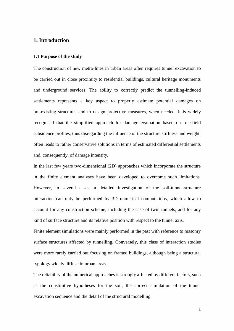
Tunnel construction is inevitably associated to ground movements which result in a

surface settlement trough developing above and ahead of the tunnel (Fig. 2.1). They are

6

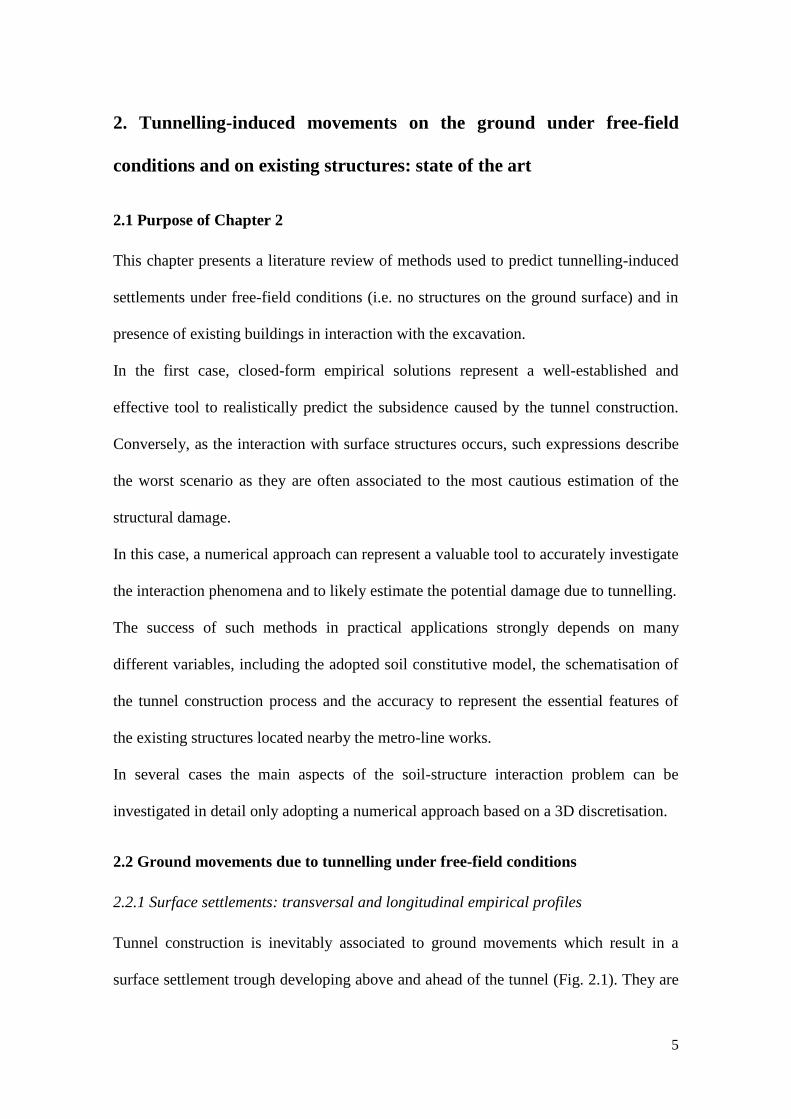
the result of different displacements occurring near the tunnel as shown in Figure 2.2

and presented in the following:

Figure 2.1. 3D settlement profile under free-field conditions (modified from Attewell et al., 1986).

Figure 2.2. Main components of ground movements due to shield tunnelling (modified from

Cording, 1991).

- component 1: face extrusion, i.e. ground displacement at the tunnel face resulting from

the stress relief associated to the excavation. This latter can be minimised by applying a

support pressure using slurry-shield or earth pressure balance (EPB) machines;

- component 2: displacement due to the shield passage. It depends on the amount of

over-excavation and it is related to the shield geometry (e.g. cutting bead thickness,

conicity) combined with the tendency of the machine, more marked in steering phases,

to plough or yaw;

7

- component 3: loss due to the tail void, i.e. the existence of a gap between the tail of the

shield and the lining which allows further radial ground movements that can be reduced

by the immediate application of grouting injections;

- component 4: lining deflection as the ground loading develops, generally smaller than

the other components if the lining is stiff enough;

- component 5: displacements due to the consolidation process in fine-grained soils.

The topic of ground movements associated with bored tunnel construction was

extensively investigated in the past by several authors and many contributions were

proposed in the literature on this theme for clays (e.g. Peck, 1969; Cording and

Hansmire, 1975; Mair, 1979; Clough and Schmidt, 1981; Ward and Pender, 1981;

O’Reilly and New, 1982; Attewell et al., 1986; Rankin, 1988; Grant and Taylor, 2000;

Loganathan et al., 1998) and for coarse-grained soils (e.g. Potts, 1976; Atkinson and

Potts, 1977; Kutter et al., 1994; Moh et al., 1996; Nomoto et al., 1995; Ata, 1996;

Celestino et al., 2000; Jacobsz, 2002; Vorster, 2005; Marshall et al., 2012).

Field observations (Peck, 1969; Schmidt, 1969), collected from many case histories

over the years, provided a description of the free-field settlement profile. At a sufficient

distance from the tunnel face, the settlement profile in a section perpendicular to the

tunnel axis (Fig. 2.3 a) can be expressed by a Gaussian distribution curve (Peck, 1969)

having the following equation:

2

22v v,max

x

xS x S exp

i

(2.1)

where:

Sv,max is the maximum settlement on the tunnel centre line;

x is the horizontal distance from the centre line;

8

ix is the horizontal distance of the inflection point of the settlement trough from the

tunnel centre line.

Figure 2.3. Transversal profiles of settlements, horizontal displacements and strains at the ground

surface (a); longitudinal surface settlement profile (b).

The volume of the surface settlement trough per meter length of tunnel, VS, can be

evaluated by integrating Equation (2.1) along the distance x to give:

2S v x v,maxV S x dx i S

(2.2)

9

The amount of volume lost in the region close to the tunnel, due to one or more of the

displacement components 1-4 of Figure 2.2, is generally indicated as VT. When

tunnelling in coarse-grained soils VT ≠ VS; in dense sands, for example, VS is less than

VT due to dilation (Cording and Hansmire, 1975). When tunnelling in clays VT = VS, as

ground movements occur at constant volume (i.e. in undrained conditions).

Of particular importance is the volume loss parameter, VL, defined as:

100%SL

t

VV

A (2.3)

where At is the nominal area of the tunnel section equal to D2/4 (D is the tunnel

diameter).

In many real cases the volume loss is a design parameter and its value is estimated on

the basis of excavation method, technological details of the tunnel boring machine

(TBM) and previous tunnelling experiences in similar geotechnical conditions. As

reported in Mair (1996), for open face tunnelling in stiff clays (e.g. London clay) the

volume loss values are generally included between 1% and 2%; for closed face

tunnelling, using earth pressure balance or slurry shields, a high degree of settlement

control can be achieved, particularly in sands where the volume loss is often as low as

0.5% and even in soft clays where, excluding the consolidation settlements, it is of only

1%-2%.

The settlement distribution can be expressed as a function of VL:

2

22

2( )

2 4x

x

iLv

x

V DS x e

i

(2.4)

O’Reilly and New (1982), in a survey of the UK tunnelling monitoring data, shown that

the point of inflection ix results approximately to be a linear function of the depth of the

10

tunnel centre line, z0, and they proposed the following simple relationship, also

confirmed by other authors (Rankine, 1988; Lake et al., 1992):

0xi K z (2.5)

where K is a constant depending solely on soil nature.

Field data collected all over the world during metro-line constructions, including shield

tunnelling, indicated that K varies between 0.2 and 0.45 for sands and gravels, between

0.4 and 0.6 for stiff clayey soils and between 0.6 and 0.75 for soft clays (Mair and

Taylor, 1997), regardless of the tunnel size and tunnelling method.

The settlement value in correspondence of x = ± ix is about 0.6 Sv,max and it is generally

accepted that the extension of the surface subsidence basin is equal to about 6 ix

(Rankine, 1988).

The inflection point divides the central part of the Gaussian curve having upwards

concavity (sagging zone) from the outer parts having downwards concavity (hogging

zone) (Fig. 2.3 a): this aspect plays a key role in the tunnelling-induced potential

damage on existing buildings, as discussed in the following.

As proposed by Clough and Schmidt (1981), the point of inflection ix can be also

influenced by the tunnel diameter. On the basis of past field data (Mair and Taylor,

1997), centrifuge data (Mair, 1979 for clays; Imamura et al., 1998 for sands and gravels)

and monitoring results, Sugiyama et al. (1999) derived the following relationships

between ix /(D/2) and the cover to diameter ratio C/D for clays (Eq. 2.6) and for sands

and gravels (Eq. 2.7):

0.8

1.5/ 2

xi C

D D

(2.6)

11

0.7

/ 2

xi C

D D

(2.7)

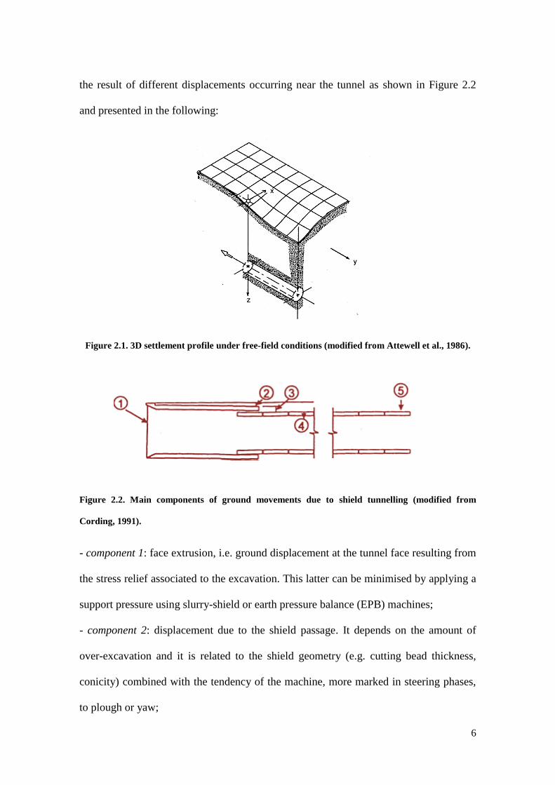
The same Authors pointed out that the data can be reasonably approximated by the

above equations, although a larger scatter is observed for sands and gravels as compared

to the clayey soils.

Other studies on coarse-grained soils shown that ix decreases with the increase in the

volume loss (Hergarden et al., 1996; Jacobsz, 2002; Vorster, 2005; Marshall et al.,

2012) due to the formation of a “chimney” mechanism (Cording, 1991), this latter also

causing the ix reduction with depth (Marshall et al., 2012). It was also observed that the

parameter ix reduces as the ratio C/D decreases (Marshall et al., 2012). In addition, it

was also noted that the Gaussian curve does not always provide a good fit to settlement

trough data in large-permeability soils (Celestino et al., 2000; Jacobsz et al., 2004;

Vorster et al., 2005), in particular in proximity to the tunnel depth (Marshall et al.,

2012).

New and O’Reilly (1991) suggested the following extension of Equation (2.5) for

tunnels constructed in layered strata of both clay and coarse-grained soils:

1

n

x i iii K z

(2.8)

where n indicates the number of the strata, Ki and zi

the trough with factor and the thickness of each layer, respectively.

The longitudinal settlement profile (Fig. 2.3 b) results to be well described by a

cumulative Gaussian probability curve (Attewell and Woodman, 1982) with the

following expression:

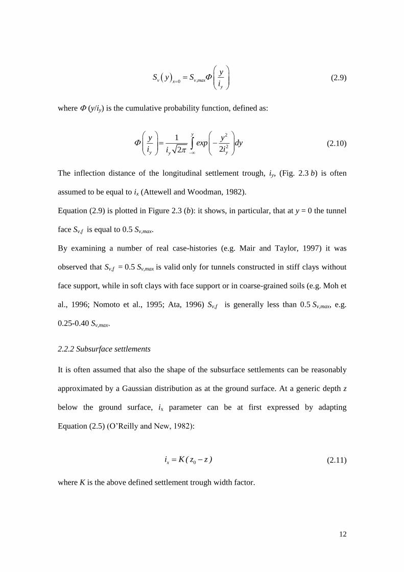
12

0v v,maxx

y

yS y S

i

(2.9)

where (y/iy) is the cumulative probability function, defined as:

2

2

1

22

y

y yy

y yexp dy

i ii

(2.10)

The inflection distance of the longitudinal settlement trough, iy, (Fig. 2.3 b) is often

assumed to be equal to ix (Attewell and Woodman, 1982).

Equation (2.9) is plotted in Figure 2.3 (b): it shows, in particular, that at y = 0 the tunnel

face Sv,f is equal to 0.5 Sv,max.

By examining a number of real case-histories (e.g. Mair and Taylor, 1997) it was

observed that Sv,f = 0.5 Sv,max is valid only for tunnels constructed in stiff clays without

face support, while in soft clays with face support or in coarse-grained soils (e.g. Moh et

al., 1996; Nomoto et al., 1995; Ata, 1996) Sv,f is generally less than 0.5 Sv,max, e.g.

0.25-0.40 Sv,max.

2.2.2 Subsurface settlements

It is often assumed that also the shape of the subsurface settlements can be reasonably

approximated by a Gaussian distribution as at the ground surface. At a generic depth z

below the ground surface, ix parameter can be at first expressed by adapting

Equation (2.5) (O’Reilly and New, 1982):

0xi K ( z z ) (2.11)

where K is the above defined settlement trough width factor.

13

However, filed measurements and centrifuge test results available in the literature for

tunnels in clay (e.g. Mair et al., 1993) indicated that K parameter increases with depth,

giving proportionally wider settlement profiles closer to the tunnel.

Mair et al. (1993) proposed the following expression, valid for tunnels in clay with

K = 0.5 at the surface, which gives a linear trend of ix parameter with depth:

0 0( ) 0.175 0.325 1 /xi z z z z (2.12)

From similar observations of subsurface settlements for tunnels in silty sands below the

water table, Moh et al. (1996) suggested this new relationship resulting in a non-linear

trend of ix parameter:

0( )

m

x

z zi z bD

D

(2.13)

where b is a constant that can be deduced by equating Equations (2.13) and (2.5) at

z = 0, while m parameter depends on the reference soils. A value of m = 0.4 was found

to fit the data for sandy soils, while m = 0.8 appeared to be more appropriate for clayey

soils.

2.2.3 Horizontal displacements and strains

Horizontal displacements are generally evaluated starting from the settlement profile

and on the basis of assumptions concerning the direction of the displacement vectors.

This allows the determination of the horizontal displacements at any point from the

settlement value at the same point using simple geometrical considerations. For tunnels

in clay in plane strain conditions and at constant volume, Attewell (1978) and O’Reilly

and New (1982) proposed that, at a generic depth z, the surface ground displacement

vectors are directed towards the tunnel axis, leading to the following simple relation:

14

0

( , ) ( , )h v

xS x z S x z

z z

(2.14)

Equation (2.14) at the ground surface can be expressed as:

2

,max 2( ) 1.65 exp

2h h

x x

x xS x S

i i

(2.15)

The theoretical maximum horizontal displacement, Sh,max, occurs at the point of

inflexion of the settlement trough (Fig. 2.3 a) and it is equal to 0.61 K Sv,max. This is

only true in undrained conditions and if K parameter is constant with depth.

The horizontal displacements are considered positive as directed towards the tunnel

axis.

Taylor (1995) shown that, for constant volume conditions, displacement vectors must be

directed towards a point located at a depth equal to 0.175z0/0.325 below the tunnel axis

and this results in a 35% reduction in surface horizontal displacements respect to those

obtained using Equation (2.14).

Attewell and Yeates (1984) introduced a parameter, n, to be applied to the numerator of

Equation (2.14) in order to take into account the variation in the focal point of the

displacement vectors to a point above or below the tunnel axis along the tunnel centre

line. They proposed values of n equal to 1 for clayey soils (undrained behaviour, i.e.

displacement vectors directed towards the tunnel centre line) and less than 1 for

coarse-grained soils (displacement vectors directed towards a point below the tunnel

centre line). This latter condition implies that in coarse-grained soils the displacement

vectors are increasingly vertical with depth and, as a consequence, the horizontal

displacements are less than those observed in clays.

The horizontal strain distribution in the transversal direction to tunnel (Fig. 2.3 a) can

be obtained by derivation of Equation (2.14):

15

2

20

( )( , ) 1v

h

x

S x xx z

z z i

(2.16)

where tensile strains are positive. In Figure 2.3 (a) the maximum values of the

horizontal strains (compressive, hc, or tensile, ht) are also highlighted.

Assuming that the displacement vectors point towards the centre of the excavation face,

the horizontal component at the surface along the tunnel centre line in the longitudinal

direction can be expressed as:

2 2

20

( ) exp8 2

Lh

y

V D yS y

z i

(2.17)

and the horizontal strains, being tensile ahead of the tunnel face and compressive behind

it, can be obtained by derivation of Equation (2.17):

2 2

2 20

( ) exp8 2

Lh

y y

V D yy y

i z i

(2.18)

2.2.4 Settlements due to twin tunnels

Many tunnelling projects in urban environments require the construction of twin tunnels

running side-by-side (e.g.: Bartlett and Bubbers, 1970; Cording and Hansmire 1975;

Harris et al., 1996) or one above the other (e.g.: Higgins et al., 1996; Shirlaw et al.,

1988).

New and O’Reilly (1991) extended the use of semi-empirical equations for predicting

the movements above a single tunnel to the case of twin tunnels, providing the

following expression:

(I) (II)2 2

2 22 2v v,max v,max

x x

x ( x d )S x S exp S exp

i i

(2.19)

16

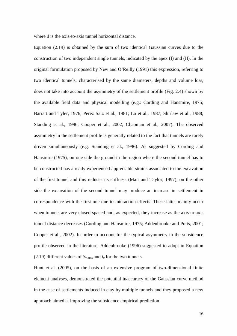
where d is the axis-to-axis tunnel horizontal distance.

Equation (2.19) is obtained by the sum of two identical Gaussian curves due to the

construction of two independent single tunnels, indicated by the apex (I) and (II). In the

original formulation proposed by New and O’Reilly (1991) this expression, referring to

two identical tunnels, characterised by the same diameters, depths and volume loss,

does not take into account the asymmetry of the settlement profile (Fig. 2.4) shown by

the available field data and physical modelling (e.g.: Cording and Hansmire, 1975;

Barratt and Tyler, 1976; Perez Saiz et al., 1981; Lo et al., 1987; Shirlaw et al., 1988;

Standing et al., 1996; Cooper et al., 2002; Chapman et al., 2007). The observed

asymmetry in the settlement profile is generally related to the fact that tunnels are rarely

driven simultaneously (e.g. Standing et al., 1996). As suggested by Cording and

Hansmire (1975), on one side the ground in the region where the second tunnel has to

be constructed has already experienced appreciable strains associated to the excavation

of the first tunnel and this reduces its stiffness (Mair and Taylor, 1997), on the other

side the excavation of the second tunnel may produce an increase in settlement in

correspondence with the first one due to interaction effects. These latter mainly occur

when tunnels are very closed spaced and, as expected, they increase as the axis-to-axis

tunnel distance decreases (Cording and Hansmire, 1975; Addenbrooke and Potts, 2001;

Cooper et al., 2002). In order to account for the typical asymmetry in the subsidence

profile observed in the literature, Addenbrooke (1996) suggested to adopt in Equation

(2.19) different values of Sv,max and ix for the two tunnels.

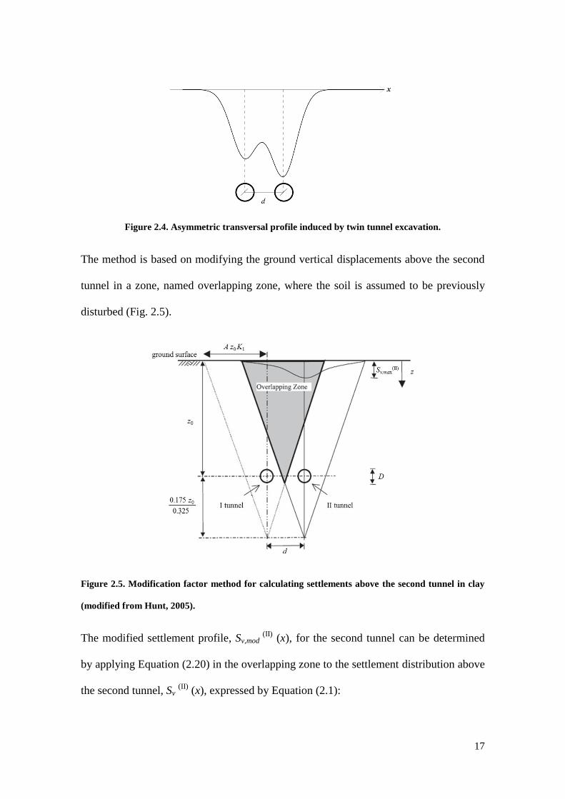
Hunt et al. (2005), on the basis of an extensive program of two-dimensional finite

element analyses, demonstrated the potential inaccuracy of the Gaussian curve method

in the case of settlements induced in clay by multiple tunnels and they proposed a new

approach aimed at improving the subsidence empirical prediction.

17

Figure 2.4. Asymmetric transversal profile induced by twin tunnel excavation.

The method is based on modifying the ground vertical displacements above the second

tunnel in a zone, named overlapping zone, where the soil is assumed to be previously

disturbed (Fig. 2.5).

Figure 2.5. Modification factor method for calculating settlements above the second tunnel in clay

(modified from Hunt, 2005).

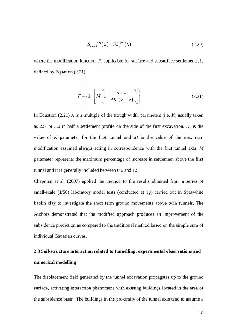
The modified settlement profile, Sv,mod (II)

(x), for the second tunnel can be determined

by applying Equation (2.20) in the overlapping zone to the settlement distribution above

the second tunnel, Sv (II)

(x), expressed by Equation (2.1):

18

(II) (II)

v,mod vS x FS x

(2.20)

where the modification function, F, applicable for surface and subsurface settlements, is

defined by Equation (2.21):

1 0

1 1d x

F MAK z z

(2.21)

In Equation (2.21) A is a multiple of the trough width parameters (i.e. K) usually taken

as 2.5. or 3.0 in half a settlement profile on the side of the first excavation, K1 is the

value of K parameter for the first tunnel and M is the value of the maximum

modification assumed always acting in correspondence with the first tunnel axis. M

parameter represents the maximum percentage of increase in settlement above the first

tunnel and it is generally included between 0.6 and 1.5.

Chapman et al. (2007) applied the method to the results obtained from a series of

small-scale (1/50) laboratory model tests (conducted at 1g) carried out in Speswhite

kaolin clay to investigate the short term ground movements above twin tunnels. The

Authors demonstrated that the modified approach produces an improvement of the

subsidence prediction as compared to the traditional method based on the simple sum of

individual Gaussian curves.

2.3 Soil-structure interaction related to tunnelling: experimental observations and

numerical modelling

The displacement field generated by the tunnel excavation propagates up to the ground

surface, activating interaction phenomena with existing buildings located in the area of

the subsidence basin. The buildings in the proximity of the tunnel axis tend to assume a

19

deformed configuration with a upwards concavity (sagging), while those farther away

from it, outside of the inflection point ix, tend to assume a deformed configuration with

a downwards concavity (hogging), as shown in Figure 2.6.

sagging hogging

Figure 2.6. Sagging and hogging deformation modes (Burghignoli, 2011).

Buildings undergoing hogging phenomena generally reveal more appreciable

resentments than those experiencing a sagging deformation. In this latter case, in fact,

the soil and the foundation system provide a constraint on the structure tending to limit

the settlement effects in its lower portion. Conversely, when a hogging phenomenon

occurs, settlements may induce larger effects in the upper portion of the structures, i.e.

where the constructions are more prone to deform.

The building deformation parameters (Burland and Wroth, 1974), widely accepted in

the literature and commonly used in soil-structure interaction studies, are shown in

Figure 2.7 considering the maximum settlement at the foundation level of four points

(i.e. A, B, C and D) and they are listed in Table 2.1.

Figure 2.7. Definition of building deformation parameters.

20

Parameter Name and Description

Sv,max maximum absolute settlement s,max maximum differential (or relative) settlement

maxmaximum slope (or rotation): maximum change in gradient of a line joining two

reference points, i.e. the ratio of their differential settlement and their distance

max angular strain: algebraic difference of slopes of two consecutive segments

max maximum relative deflection: maximum displacement of a point relative to the line

connecting two reference points on either side

(L)maxmaximum deflection ratio, where L is the distance between the two reference

points defining max

rigid body rotation of the whole structure

max maximum value of the angular distortion: difference between max and

Table 2.1. Structural deformation parameters.

2.3.1 Experimental observations

The conventional approach to evaluate possible tunnelling-induced damage, currently in

use for a preliminary assessment of building performance, is based on the empirical

prediction of the subsidence curve under free-field conditions (Peck, 1969; O’Reilly and

New, 1982), neglecting any effect due to the presence of surface structures on the

displacement field. The constructions resting on the ground, in fact, may modify the

shape of the subsidence profile due to their stiffness and weight, generally reducing the

differential settlement.

Breth and Chambosse (1974) shown field data for reinforced concrete framed buildings

undercrossed by twin tunnel excavation in Frankfurt Clay, highlighting that they exhibit

a different response: the structure deforming in sagging shows a more flexible

behaviour with respect to that undergoing hogging.

Viggiani and Standing (2002) analysed settlements induced by the construction of the

Jubilee Line Extension tunnels in London Clay, comparing the measurements recorded

at the Treasury Building with those obtained in a nearby free-field section. The

differential settlements under the structure result significantly smaller than the free-field

ones, due to the building stiffness. Absolute settlements of the structure are smaller than

21

those measured at the ground in the sagging zone, while they are slightly larger in the

hogging portion of the subsidence profile.

Mair (2003) presented measurements of settlements recorded in correspondence with an

ordinary masonry building, named Neptune House, in interaction with the construction

of twin tunnels, in order to highlight the stiffer response of the structure in the sagging

zone. This experimental evidence confirms what observed by Burland et al. (1977)

regarding the more flexible response of masonry buildings that experiment hogging

deformation and what discussed by Son and Cording (2005), referring to the

experimental results of scale model tests of masonry façades adjacent to deep

excavations.

Dimmock and Mair (2008) analysed the settlement response of 2 and 3-storey masonry

structures founded on shallow strip foundations. The observed settlement profiles of the

Moodkee Street and Keetons Estate buildings, when compared to the equivalent

free-field ones, reveal that these structures display close to fully flexible behaviour in

hogging, but they are semi-flexible in sagging. The horizontal strains measured at the

base of the building façades are negligible, indicating the high axial stiffness of these

masonry buildings.

Many other Authors (e.g. Cording and Hansmire, 1975; Geddes and Kennedy, 1985;

Boscardin and Cording, 1989; Viggiani and Standing, 2001; Withers, 2001; Mair, 2003)

analysed the response of buildings resting on continuous foundations in interaction with

tunnel excavations, concluding that such structures are interested by very small

horizontal deformations with respect to what observed under free-field conditions.

Goh and Mair (2010) presented a case-history on the settlement response of two

reinforced concrete framed buildings above the bored tunnelling works for a section of

the Singapore Circle Line, showing that the framed building stiffness can influence their

22

response to excavation. The Authors proposed a method to quantify this influence based

on the definition of a factor (named column stiffening factor) which puts in relation the

bending stiffness of a framed building to that of a simple beam for which the deflection

ratio can be estimated following the approach presented by Potts and Addenbrooke

(1997) and discussed in the next Section 2.3.2.3.

Referring to the same case-study, Goh and Mair (2011) shown that the horizontal strains

are significantly reduced for most buildings on continuous footings, while for structures

on individual footings the horizontal strain values correspond to those under free-field

conditions. The Authors illustrated the difference in horizontal strains between columns

that are connected by ground beams and columns that are unconnected at ground level,

but connected at first floor upwards. Using a combination of simplified structural

analysis and finite element models, a design guidance was proposed to estimate

excavation-induced horizontal strains in framed buildings on individual footings.

Farrell et al. (2011) analysed the response of 2 and 5-storey commercial masonry

buildings with reinforced concrete floor slabs founded on strip footings and located in

proximity to the excavation of a tunnel having a diameter equal to 12 m. The 5-storey

building is characterised by larger vertical displacements when compared to the ground

settlements recorded at a nearby control section, due to its stiffness and weight, while

the 2-storey structure exhibits a more flexible response, deforming according to the

free-field subsidence profile.

2.3.2 Numerical modelling

The use of two-dimensional (2D) and three-dimensional (3D) numerical approaches,

developed in the last few years and nowadays common, allows a more realistic analysis

of the soil-tunnel-structure interaction process. However, the success of such methods

(finite-element or finite-difference methods) in practical application strongly depends

23

on different factors, including the constitutive hypotheses adopted for the soil, the 2D or

3D schematisation of the tunnel excavation sequence and the detail in modelling the

structures in interaction with the tunnel.

2.3.2.1 Soil constitutive models

It is widely recognised that soil exhibits much higher stiffness at very small strains (e.g.

strains ≤ 1 x 10-6

) than that measured in traditional laboratory tests on soil specimens.

As the strain increases, the soil stiffness decays non-linearly and this feature,

represented by the characteristic S-shaped stiffness reduction curve (e.g. Vucetic and

Dobry, 1991), is incorporated into some constitutive models of soil behaviour proposed

in the literature.

The first small-strain models for static applications were introduced by Mroz et al.

(1981) and Burland et al. (1979) that used kinematic yield surfaces in the stress space

and in the strain space, respectively.

Parallel to these models with kinematic surfaces, a different approach was proposed by

Jardine et al. (1985, 1986) that, by fitting the strain-stiffness curves, directly calculate

the soil stiffness as a mathematical function of the applied strain.

Al-Tabbaa (1987) presented the innovative idea of a very small inner yield surface,

named bubble, and Al-Tabbaa and Wood (1989) published the two-surface bubble

model as an extension of the Cam Clay model. Stallebrass (1990) introduced an

additional history surface for the bubble extension within the Cam Clay framework.

Then, a three-surface kinematic hardening model (3-SKH), able to simulate the

non-linearity and the effect of recent stress history, was developed by Stallebrass and

Taylor (1997).

Advanced mathematical descriptions of the strain-stiffness curve following the

approach by Jardine et al. (1986) were proposed by Gunn (1993) and Tatsuoka (2000).

24

During the last few years, kinematic hardening models were further extended to take

into account the effect of structure in natural soils (e.g. Rouainia and Muir Wood, 2000;

Kavvadas and Amorosi, 2000; Baudet and Stallebrass, 2004). Grammatikopoulou et al.

(2006) presented two new kinematic hardening models, which modify the pre-existing

two-surface (Al-Tabba and Wood, 1989) and three-surface (Stallebrass and Taylor,

1997) models. The novelty consists in a hardening modulus resulting in a smooth

elasto-plastic transition and in a realistic stiffness degradation curves.

A kinematic-hardening structured soil model incorporating structure and stiffness

degradation was presented by Gonzalez et al. (2012) and used in numerical analyses

performed to simulate the undrained excavation of a tunnel in London Clay. The work

highlights as the choice of a representative small-strain stiffness value in the model

calibration requires a considerable amount of engineering judgment.

Benz (2007) proposed an isotropic-hardening elasto-plastic constitutive model, named

Hardening Soil model with small-strain stiffness (HSsmall), that represents an extension

of the Hardening Soil Model (HS) previously developed by Shanz et al. (1999) and

which is capable of taking into account the very high soil stiffness at very low strain

levels, its variation with the strain level and the early accumulation of plastic

deformations.

2.3.2.2 Tunnelling process: 2D and 3D numerical simulations

2D numerical simulation

Tunnelling process is characterised by a three-dimensional nature and this peculiarity

has to be taken into account when the excavation is simulated by two-dimensional

numerical analyses frequently adopted in engineering practice, assuming plane strain

conditions.

25

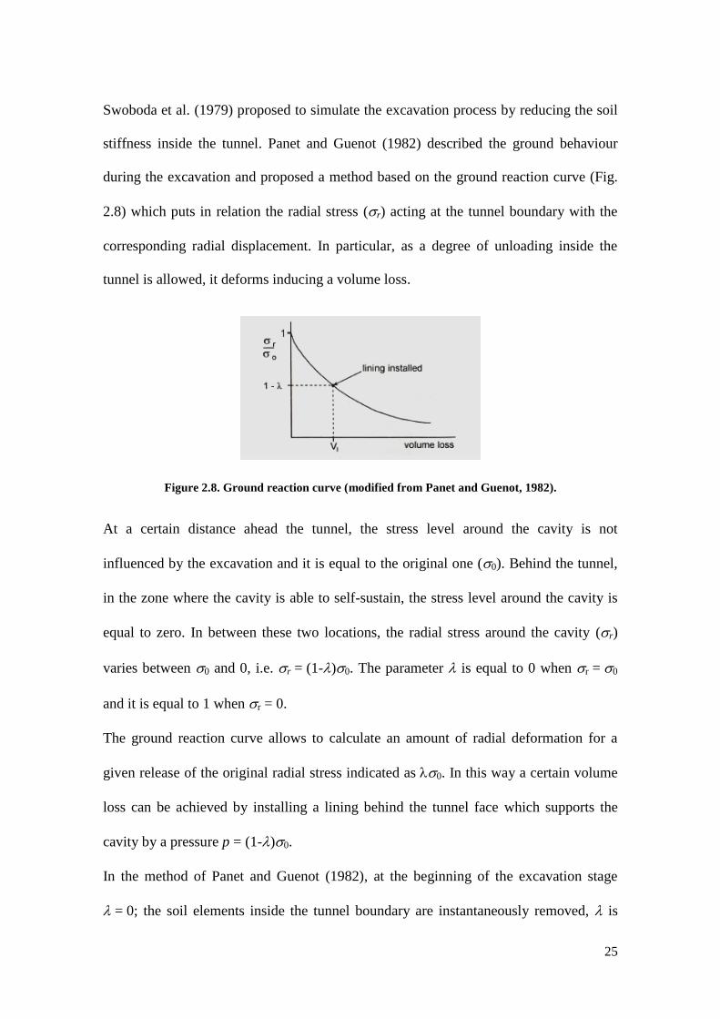
Swoboda et al. (1979) proposed to simulate the excavation process by reducing the soil

stiffness inside the tunnel. Panet and Guenot (1982) described the ground behaviour

during the excavation and proposed a method based on the ground reaction curve (Fig.

2.8) which puts in relation the radial stress (r) acting at the tunnel boundary with the

corresponding radial displacement. In particular, as a degree of unloading inside the

tunnel is allowed, it deforms inducing a volume loss.

Figure 2.8. Ground reaction curve (modified from Panet and Guenot, 1982).

At a certain distance ahead the tunnel, the stress level around the cavity is not

influenced by the excavation and it is equal to the original one (0). Behind the tunnel,

in the zone where the cavity is able to self-sustain, the stress level around the cavity is

equal to zero. In between these two locations, the radial stress around the cavity (r)

varies between 0 and 0, i.e. r = (1-)0. The parameter is equal to 0 when r = 0

and it is equal to 1 when r = 0.

The ground reaction curve allows to calculate an amount of radial deformation for a

given release of the original radial stress indicated as0. In this way a certain volume

loss can be achieved by installing a lining behind the tunnel face which supports the

cavity by a pressure p = (1-)0.

In the method of Panet and Guenot (1982), at the beginning of the excavation stage

= 0; the soil elements inside the tunnel boundary are instantaneously removed, is

26

incrementally increased up to a given value and, at this point, the lining is activated.

Then, is further increased until to 1 at the end of excavation.

In the gap method of Rowe et al. (1983) a predefined vertical distance, called “gap”

parameter, is imposed in the finite element mesh between the tunnel profile and the

lining to represent the expected volume loss.

In the method presented by Vermeer and Brinkgreve (1993) the volume loss is

simulated by applying a contraction to the lining: in the first phase of the numerical

procedure, the soil is removed and the lining installed at the same time, while in the

second one a contraction is imposed to the lining in order to obtained a reference value

of VL.

In the volume loss control method proposed by Addenbrooke et al. (1997) the tunnel

excavation is modelled in n increments. The volume loss value is evaluated at each step

and the lining elements are activated when the desired VL is obtained.

It was also shown by the same Authors that for soils characterised by a coefficient of

earth pressure at rest K0 > 1 the computed settlement profiles are wider than real

observations and empirical predictions for the same values of the volume loss. Referring

to the case of overconsolidated clays (i.e. London Clay), they proposed an improvement

of the settlement numerical prediction by fictitiously altering the soil parameters and

introducing an unrealistically low anisotropy ratio Gvh/E′v, these latter being the shear

stiffness and Young’s moduli in the vertical direction, respectively. An alternative

approach used by the same Authors consists in introducing a fictitious zone of reduced

K0 around the tunnel before simulating the excavation process.

An extension of the method proposed by Rowe et al. (1983) was presented by

Tamagnini et al. (2005). It includes an ovalisation of the tunnel profile which provides a

good agreement among numerical predictions, empirical relations and measurements.

27

A numerical schematisation of tunnelling inspired by the methods of Panet and Guenot

(1982) and Addenbrooke (1997) was proposed by Altamura et al. (2007). In this

procedure, the vertical and horizontal component of initial equilibrium nodal forces are

independently released on the tunnel boundary until an adequate vertical to horizontal

release ratio, calibrated for the single case, is found.

The computed settlement profiles result in good agreement with the empirical curves

calculated for the same volume loss using realistic values of K parameter.

In the method proposed by Moller and Vermeer (2008), settlements are controlled by

the simulation of the grouting action in the void between the lining and the soil.

3D numerical simulation

In several cases, the main aspects of the interaction between tunnels and existing

buildings can be investigated only by adopting a numerical approach based on a 3D

discretisation, which allows to capture the real geometry of the abovementioned

soil-structure interaction problem. In this context, the correct 3D schematisation of all

the excavation, support and lining sequences plays a key role for a realistic prediction of

the subsidence phenomena.

In the past, the first 3D numerical simulations of tunnelling process were drastically

simplified. Augarde et al. (1999) and Burd et al. (2000) proposed the simultaneous

excavation method: tunnel excavation is simulated in a single step by removing the soil

elements inside the tunnel boundary up to the desired face position and by

simultaneously installing the lining over the whole excavated length. Subsequently, a

uniform contraction is applied to the lining along the whole length. This method

overcomes the geometry limitations of 2D analyses, but it simulates only in part the

excavation sequence as a 3D process. It produces settlement trough widths larger than

those predicted by the empirical equation for the same volume loss values.

28

Several Authors (e.g. Tang et al., 2000; Franzius, 2003; Franzius and Potts, 2005;

Möller, 2006) used a step-by-step method to simulate the excavation process. In

general, it consists in removing at each calculation step the soil elements inside the

excavation profile over a length, indicated as Lexc, ahead of the tunnel face and in

activating the lining at a certain distance behind the face, this latter being supported by a

pressure acting on it. In some cases a support pressure, or a displacement field, may be

also applied to the unsupported soil between the lining and the excavation face.

In a more recent version of this method available in the literature (Rampello et al.,

2012), the tunnel cavity is lined by the shield or by the permanent lining, with the

exception of the tunnel face, where a support pressure equal to the total horizontal stress

at rest is applied, and of an intermediate 4 m long zone, where the displacements are

forced. The shield extends for a total length of 8 m and the permanent lining is installed

behind the shield. Tunnelling is modelled in discrete steps by removing a 2 m long slice

of soil and advancing the support pressure, the shield and the lining by the same length.

Values of the maximum displacement, δ, imposed at the tunnel crown are determined by

trial and error to meet the requirement that the design volume loss is achieved after the

completion of the tunnel. The settlement troughs computed at the surface by the

numerical analyses performed using the above described tunnelling sequence, in

general, compare well with those given by the empirical procedure, both in terms of

maximum settlement and width of the subsidence basin.

Examples of very realistic shield tunnelling simulation, capable of reproducing and

explicitly modelling many details of the process (e.g. shield geometry, magnitude and

distribution of the face support pressure, hydraulic jack thrust, volume and pressure of

the grouting injections, etc.), were proposed in the literature (e.g. Komiya et al., 1999;

Kasper and Meschke 2004, 2006 a, 2006 b). In some cases it emerges that such

29

complex simulations may give realistic results when combined with advanced

constitutive hypotheses adopted for the soil.

Further research works (e.g. Melis et al., 2002; Migliazza et al., 2009; Lambrughi et al.,

2012) compared numerical analyses with recorded data and explored the role of

different shield-tunneling parameters on the surface settlements and stresses developed

on the final lining. An extension of these methods to a full interaction of the TBM-EPB

process was presented by Comodromos et al. (2014). In this case, the excavation

process was simulated by a step-by-step procedure and the face support pressure, the

tunnel lining, the tail gap grouting, the shield and the over-excavation were modelled in

the numerical scheme. The influence of almost all relevant components of shield

tunnelling was assessed by a parametric study and the sensitivity of the process to

variations of the face support, of the pressure applied to the steering gap slurry and of

the tail gap grouting was examined. It was found that the tunnel face pressure has the

most influence on the surface settlements, while the steering and tail gap pressures

affect the ground movements in a non-relevant way.

2.3.2.3 Numerical analysis of the interaction between structures and tunnels: 2D and

3D approaches

Numerical methods represent an attractive solution for the evaluation of the complex

soil-tunnel-structure interaction phenomena which can be investigated by several

approaches characterised by a different level of complexity.

In general, a fully-coupled approach is the most satisfactory tool, as it explicitly

includes in the same numerical scheme all the ingredients of the problem: the soil, the

tunnel and a full structural model of the building (e.g. Amorosi et al., 2014). Thus, it

allows a direct estimation of the stress and strain fields acting in the structure and of the

damage induced by the excavation process.

30

An alternative and strongly simplified uncoupled approach can also be employed,

generally at the preliminary stage of the analysis. In this method, characterised by a

limited computational effort, the displacements predicted under free-field conditions are

simply applied at the base of the building. Separate numerical models are used for the

soil and for the structure (e.g. Maleki et al., 2011), while their interaction is studied by

an iterative process.

An intermediate solution is represented by a semi-coupled (or partly-uncoupled)

approach (e.g. Losacco, 2011; Rampello et al., 2012, Losacco et al., 2014) that,

although requiring a soil-structure interaction analysis, introduces a simplified

equivalent model of the building. This method, limiting the required computational

power and the calculation times, can be useful to investigate specific cases, for example

the simultaneous effect of tunnelling on many existing buildings.

As will be discussed in the following, soil-structure interaction problems were explored

by 2D or more advanced 3D numerical studies presented in the literature, frequently

devoted to analyse the response to tunnelling of masonry buildings and, more rarely, of

reinforced concrete framed structures.

2D approach

In the first studies aimed at investigating the structural response to ground settlements,

the building was represented by a simple, weightless, 2D deep elastic beam undergoing

sagging and hogging modes of deformation according to the soil displacement profile;

the onset of cracking was related to the critical tensile strain within the beam associated

with shear and bending modes of deformation (Burland and Wroth, 1974; Burland et al.,

1977). This model was then improved to incorporate the influence of the horizontal

strain (Boscardin and Cording, 1989; Burland, 1995).

31

An attempt to overcome this uncoupled approach, that disregards not only the mutual

interaction between the soil and the structure, but also the influence of this latter on the

tunnelling-induced soil movements, was proposed by Potts and Addenbrooke (1997), on

the basis of a parametric finite-element study representative of the typical conditions

encountered during tunnel excavations in London Clay. Their study involved more than

100 non-linear numerical analyses where the surface framed structure is modelled by an

equivalent weightless beam located on the ground and characterised by different values

of width, stiffness and eccentricity with respect to the tunnel axis. The results show that

both the axial and bending stiffness of the beam influence the ground displacement

field, this latter being very different to the free-field one. The presence of a structure has

the effect of reducing settlements as compared to the free-field scenario; however, the

vertical displacements can be larger than those evaluated without structure if this latter

is characterised by a low bending stiffness and a realistic axial stiffness. The Authors

defined two parameters, named relative bending stiffness (*) and relative axial stiffness

(*); these parameters take into account the soil-structure relative stiffness and the so

called modification factors for the deflection ratio (MDR

) and for the horizontal strain

(Mh

), which indicate as the structure modifies the free-field predictions of the relevant

damage parameter. The design curves introduced by Potts and Addenbrooke (1997) in

the assessment process of the building damage enable a more accurate prediction of the

likely damage to existing structures.

Rampello and Callisto (1999) examined the case of a tunnel excavation in silty-sand

passing under Castel Sant’Angelo in Rome (Italy), a massive masonry monumental

building whose inner portion is of Roman age. In their work the structure is modelled as

an isotropic linear elastic-perfectly plastic material with limited compressive strength

and no tensile strength, while the soil behaviour is described by two different

32

constitutive models (i.e. an elastic-perfectly plastic model and an elastic-plastic model

with isotropic deviatoric hardening). The results of the numerical analyses show that the

high stiffness of the building plays a major role in the interaction process. The evaluated

potential damage induced by tunnelling on the structure is shown to be significantly

influenced by the choice of the soil constitutive model.

Liu et al. (2000) also used a continuum approach to study the response of masonry

façades to tunnel excavation in London Clay, using a non-linear model for both soil

(Houlsby, 1999) and surface building. In particular, the masonry material, elastic in

compression, can crack when it reaches its tensile strength. Their study involves

comparison of crack patterns obtained on plane stress façades by coupled and uncoupled

analyses; in this latter case, the displacement filed obtained by a previous free-field

analysis is applied at the base of the façade. Their analysis concentrates on the effects of

the façade weight and stiffness and of the horizontal location of the façade with respect

to the tunnel axis, finding that increasing weight tends to increase the damage, owing to

larger horizontal strains. Increasing façade stiffness, however, appears to reduce the

damage, since the differential settlements under the façade result inhibited.

Boonpichetvong and Rots (2002) presented the application of fracture mechanisms to

predict the cracking damage in masonry buildings subjected to ground movements by

tunnelling activity. They described the computational approach employed to capture the

failure mechanism of a selected historical masonry façade, typical for the western part

of The Netherlands. The soil-structure interaction process is studied by a finite element

approach, testing various continuum crack models in large-scale fracture analyses. The

results indicate some limitations of the utilised crack models in predicting the settlement

damage, highlighting the need for reliable numerical techniques for highly brittle

material.

33

Melis and Rodrìguez Ortiz (2003) illustrated a method of establishing the stiffness of

several types of buildings (i.e. masonry buildings, framed buildings in steel or

reinforced concrete) taking into account their main structural elements. The resulting

values allow to model the reference structure as an equivalent beam with an associated

modulus of deformation. This procedure was applied to a real case of study, i.e. the

construction of the metro-line 7 of Madrid (Spain) by EPB-tunnelling, analysed by a

finite element approach. The tunnel passes through hard and stiff soils, interacting with

structures of different type. Actual observations confirm that stiff buildings rarely suffer

damage, this latter being associated with very high angular distortions for the more

flexible ones.

The response of buildings with different structural types resting on shallow foundations

subjected to excavation-induced ground settlements was also compared by Son and

Cording (2011), providing a better understanding of the complex soil-structure

interaction in building response. The investigated structures include brick-bearing

structures, open-frame structures and brick-infilled frame structures, that are often

encountered near a construction area. In their research, numerical studies, performed by

the distinct element method (DEM), were carried out to evaluate the response of such

buildings subjected to an identical progressive ground settlement and to provide key

features of their response in different soil conditions.

The structural behaviour was investigated using distortions and crack damages induced

to the structures by ground settlements. Results indicate that such a response is highly

dependent on structural type, cracking in a structure and soil condition, highlighting that

their effects should be considered to better assess the potential damage due to

tunnelling-induced ground subsidence.

34

In general, if the same magnitude of ground settlement occurs, a structure on stiffer soil

is more susceptible to building damage caused by ground settlement than a structure on

softer soil. This latter has a tendency to modify the ground settlement profile and

undergoes less distortion. However, the effect of soil stiffness decreases when a

structure has enough strength or it is restrained by some elements such as the frames in

a brick-infilled framed structure. In particular, as cracking occurs in a brick-bearing

structure, the subsequent cracks concentrate around the initial ones and propagate

farther out with advancing ground settlements. However, for a brick-infilled framed

structure the enclosed frame significantly confines the crack propagation, so that the

structure undergoes relatively small distortion regardless of its conditions.

A finite element semi-coupled model including a cracking low for the masonry and a

non-linear interface simulating the soil–structure interaction, was validated against

experimental results (Giardina et al., 2012) by Giardina et al. (2013). The aim of this

work is to produce a reliable validated numerical approach to improve the current

procedures for the assessment of tunnelling-induced damage to masonry structures. The

emphasis is on the crack modelling and on the robustness of the analysis for a critical

case of a brittle façade on an elastic bedding. In particular, the feasibility of a continuum

approach for the crack modelling of masonry was evaluated and, considering the

convergence difficulties related to the non-linear modelling of quasi-brittle material, a

new sequentially linear analysis scheme was also proposed. In comparison with

previous works (e.g. Son and Cording, 2005), this study offers an evaluation of the

structural damage evolution as a function of the applied deformation throughout the

entire experimental and numerical tests, obtaining in this way new empirically validated

results.

35

Alongside the same topic, Giardina et al. (2014) examined the masonry response to

tunnelling by a sensitivity study on the effect of cracking and building weight. With the

aim to improve the useful existing procedures for predicting damage due to tunnelling,

their research considers the use of a finite element modelling, including non-linear

constitutive laws for the soil and the structure, to analyse the response of a masonry

structure, represented by a simple beam, subjected to tunnel excavation in sand. The

numerical model was validated through a comparison with a series of centrifuge tests

(Farrell, 2010). Results indicate a general increase in the beam deflection ratio with

weight, suggesting a direct correlation between this latter, normalised to the relative

stiffness between the structure and the soil (Potts and Addenbrooke, 1997), and the

modification of the settlement profile. The weight can reduce the effect of an increment

in relative stiffness and it is more evident for relatively high values of the volume loss

and beam stiffness. A variation in the modified deflection ratio is also observed when a

cracking model for masonry is included in the simulations, depending on the initial

stiffness and material parameters.

The analysis of deformation and damage mechanisms induced by shallow tunnelling on

masonry structures was carried out by Amorosi et al. (2014). The study, conducted by

the finite-element code Abaqus, was performed in 2D conditions assuming plane strain

and plane stress conditions for the soil and the structure, respectively.

As such, the analysed class of problems is that of a tunnel excavated under a masonry

structure, this latter being characterised by its plane oriented perpendicularly to the

tunnel axis.

The modelled structure represents an ancient masonry wall, schematised as a block

structure with periodic texture and characterised by a non-linear anisotropic mechanical

36

response. The soil was modelled using a conventional linear elastic-perfectly plastic

Mohr-Coulomb model.

The Authors performed a preliminary parametric study on the behaviour of a simple

masonry structure affected by the excavation of a shallow tunnel, aimed at investigating

the influence of the mechanical and geometrical properties of the structure. The

numerical analyses carried out with different values of mortar joints’ cohesion (0, 5 and

10 kPa) clearly demonstrate the role of the non-linear structural behaviour on the correct

assessment of the masonry response. In particular, the influence of structure cohesion

appears negligible in terms of overall settlement pattern, but more relevant for the

damage development within the masonry wall. The analysis for a null cohesion displays

a severe shear-induced damage pattern, while no significant differences are observed

between the analyses carried out with cohesion values of 5 and 10 kPa.

A linear anisotropic-elastic analysis would have predicted the same level of damage in

all the investigated cases.

Free-field preliminary analyses demonstrate that, despite the relatively simple

constitutive hypothesis adopted for the soil, the displacement-controlled technique used

in the study to reproduce the tunnel construction well captures the induced ground

displacements, as highlighted by the comparison with the Gaussian curves for surface

settlements at different volume losses. The numerical results are able to mimic the main

features of the soil–structure interaction, including the modifications in the subsidence

profile and the related deformative pattern in the structure.

In the same work the Authors presented a numerical back-prediction of the settlements

induced in a complex historical masonry structure (the Felice Aqueduct in Rome, Italy)

by the excavation of shallow twin tunnels. First, an uncoupled analysis was performed,

by applying at the base of the structure the displacements obtained by the model under

37

free-field conditions. Then, a fully coupled simulation was carried out, thus highlighting

the influence of soil–structure interaction on the computed deformative response of the

structure, characterised by a reduced amount of tensile plastic strains, and in the ground,

where horizontal displacements were dramatically decreased. In order to test the

numerical approach, the computed ground and structural surface vertical displacements

were compared with monitoring data. Numerical outcomes result to be in good

agreement with experimental data, thus validating the numerical model for this class of

soil–structure interaction problems.

3D approach

The effects of the weight and stiffness of surface structures on the ground settlements

were studied by Burd et al. (2000) using a three-dimensional finite element analysis in

which the tunnel, the soil and a masonry building were all included in a single

numerical model. Although three-dimensional, the geometry of the problem is relatively

simplified: the structure, in fact, consists of two identical façades, connected by two

plane walls, with openings to model the windows and the door, while the roof, the

floors, the internal walls and the foundation details were neglected. The excavation

process of an unlined tunnel was simulated by incrementally removing the soil elements

within a predefined zone. A multi-surface plasticity model (Houlsby, 1999) was adopted

in the numerical study to describe the non-linear and irreversible behaviour of the soil,

while a relatively straightforward model was assumed for masonry in which the

material has a low tensile strength and infinite compressive strength. The presented

results illustrate the mechanisms of interaction between the building and the ground

considering two different tunnel positions (symmetric and non-symmetric with respect

to the structure). In particular, it was pointed out that the performance of the building

results highly dependent on the deformation mode: for façades subjected to sagging

38

deformation the soil-structure interaction process allows to reduce the predicted

tendency of the building to suffer settlement-induced damage, while when the building

deforms in a hogging mode, it results less effective in reducing the differential

settlements.

Mroueh and Shahrour (2003) presented a numerical study of the interaction between a

lined tunnel and an adjacent reinforced concrete structure conducted by a full

three-dimensional calculation which takes into account the presence of the structure

during tunnelling. The tunnel construction process was modelled by a simplified

step-by-step procedure and the structure was schematised as a spatial frame composed

by columns and beams. The soil behaviour was assumed to be governed by an elastic

perfectly-plastic constitutive relation based on the Mohr–Coulomb criterion with a

non-associative flow rule and the behaviour of the structure was assumed to be

linear-elastic. The proposed study confirms that tunneling-induced movements are

largely influenced by the presence of adjacent structures, showing as the simplified

approach, which considers the free-field soil movements for the evaluation of structural

damage, results very conservative. The performed numerical study also highlighted the

importance of considering the building self-weight in the determination of the initial

stress in the soil before tunnelling.

The soil-structure interaction phenomenon was also examined in the coupled numerical

study proposed by Jenck and Dias (2004) who, however, considered all the component

of the process in a simplified way. In particular, in their study the soil behaviour is

elastic-perfectly plastic, the tunnel excavation is a simplification of the real phases of

the TBM process based on the concept of volume loss and the reference building is an

ideal reinforced concrete structure, with no eccentricity respect to the tunnel, founded

on a raft foundation and composed by columns and floors. The main aim of the study is

39

the analysis of the role of the structural stiffness on the soil surface displacements. It

was found, in accordance with previous studies, that the presence of the structure leads

to negligible horizontal displacements under its foundations as compared to the

free-field calculations and, consequently, the application of the free-field deformations

to the building for damage estimation results to be conservative. This study also pointed

out that the larger the building stiffness, the smaller the surface differential settlements.

Similar results were presented in the 3D numerical study proposed by Keshuan and

Lieyun (2008). Their research is based on a finite element model which takes into

account the presence of a strongly schematised spatial framed structure during the

excavation of twin tunnels. A very simple structural scheme, consisting of beams,

columns and live loads acting at each floor of the reinforced concrete building was also

proposed by Liu et al. (2012) for the numerical analysis of ground movements due to

metro-station driven with enlarging shield tunnels.

A finite element study aimed at demonstrating the importance of 3D modelling to

evaluate the influence of the excavation advancement and tunnel-building relative

position on damage mechanism was presented by Giardina et al. (2010). The Authors

proposed a coupled scheme taking into account a damage model for the masonry

building and the non-linear behaviour of the soil-structure interface. This latter was

adopted to simulate the transmission of vertical and horizontal deformations from the

ground to the structure through the shallow strip foundations. The structure, subjected to

dead and live loads, only consists of external façades with openings and internal walls;

the roof and the floor diaphragms were not represented due to their negligible stiffness

with respect to that of the global building. The tunnelling process was simulated by

subsequent stages of soil excavation and lining installation. The Authors investigated

the effect of different factors (such as the expected volume loss and the location of the

40

building with respect to the tunnel) on the shape of the settlement profile. They also

highlighted that crack pattern and failure mechanism evolve in the structure during

tunnelling, pointing out, in particular, the importance of a three-dimensional description

of the tunnel excavation process and building geometry for a complete analysis of the

structural damage.

In the literature, several Authors defined simplified structural models with the aim to

reproduce the behaviour of masonry or reinforced concrete buildings in the interaction

analyses.

Franzius et al. (2006) proposed an extension of the study presented by Potts and

Addenbrooke (1997), this time considering the building as an equivalent elastic shell

with weight. The evaluation of the equivalent structural stiffness employs the parallel

axis theorem, likely overestimating the stiffness of a real structure. In the proposed

method the foundation system is not taken into account reducing, in contrast, the overall

stiffness. Such methodology, however, is based on certain assumptions regarding the

structural typology: it is mostly applicable to the buildings characterised by geometrical

regularity, while it results not appropriate to those with more complicated features. This

schematisation, for example, was applied in the theoretical study presented by Maleki et

al. (2011) aimed at investigating the effect of structural characteristics (i.e. geometry,

stiffness and weight) on tunnel-building interaction.

In the finite element procedure proposed by Pickhaver et al. (2010) to evaluate the

structural damage due to tunnelling, the masonry building is represented in an

approximate way by equivalent elastic Timoshenko beams. The Authors discussed the

method to estimate the appropriate properties for the equivalent beams in terms of

flexural and shear stiffness. The procedure is shown to compare favorably with the

41

results of a parametric numerical study of a range of building façades and internal wall

subjected to applied displacements along their base.

The performed analyses shown that the response of the equivalent beams provides a

good match with that of the masonry façades, modelled using a non-linear constitutive

model, in the case of sagging deformation, while the proposed structural simplification

requires the use of a reduced flexural stiffness to match the more flexible response of

masonry panels which deform according to a hogging mode.

Rampello et al. (2012) illustrated the procedure adopted to evaluate the effect of

tunnelling on existing monuments and historical buildings, with particular reference to

the construction of the metro-line C of Rome (Viggiani and Soccodato, 2004; Losacco,

2011; Burghignoli, 2011). Specifically, the study of the interaction between

construction activities and the built environment was carried out following two

procedures at increasing levels of complexity: at the first level, free-field analyses were

carried out neglecting the stiffness of the existing buildings for a simplified evaluation

of the potential damage induced by tunnel excavation; at the second level, an interaction

numerical study was performed accounting for the stiffness of existing buildings

modelled in a simplified way.

The main aspects of such procedure were illustrated using, as an example, the

case-study of Palazzo Grazioli. The mechanical behaviour of the soil was described by

an elasto-plastic constitutive model with isotropic hardening and Mohr-Coulomb failure

criterion (i.e. the Hardening Soil model), while the reference structure was modelled as

an equivalent solid with simpler geometry and appropriate mechanical properties. This

equivalent solid is fully embedded into the soil and it is assumed to behave as a

linear-elastic material. This latter assumption may be valid only for relatively small

volume loss, that is when the structure undergoes small distortions. In the simple

42

hypothesis of isotropy, the mechanical behaviour is completely described by the

Poisson’s ratio and Young’s modulus. It is postulated that the actual and the simplified

structures are equivalent if they show a similar response to a given perturbation, which

consists in imposing the vertical displacements computed in the free-field analyses at

the foundation level; the corresponding response is the distribution of the nodal forces at

the same level. The Young’s modulus of the equivalent solid is found iteratively, to

produce a distribution of nodal forces at foundation level that matches the distribution

computed using a complete structural model of the building.

In a subsequent step, the equivalent solid is introduced in the finite element model with

its equivalent stiffness and weight reproducing those of the complete building. The

numerical analyses produce a new displacement field, accounting for the stiffness and

weight of the building, that is eventually applied to the complete structural model for a

final evaluation of the effects induced by tunnel construction.

The study highlights the importance of a three-dimensional interaction analysis in cases

of geometrical complexities. As a general result, explicit consideration of stiffness and

weight of the building leads to larger settlements but smaller distortions, and therefore

to a predicted less damage than the free-field analysis.

2.4 Evaluation of building damage

2.4.1 Damage classification

The control of tunnelling-induced ground movements and the protection of the built

environment from potential damage represent the principal design and construction

requirements (Viggiani and Soccodato, 2004). The ability to predict with confidence the

displacements due to tunnelling is a crucial aspect as ground movements transmit to

adjacent structures as settlements, rotations and distortions of foundations which can

induce damage affecting visual appearance and aesthetics, serviceability or function

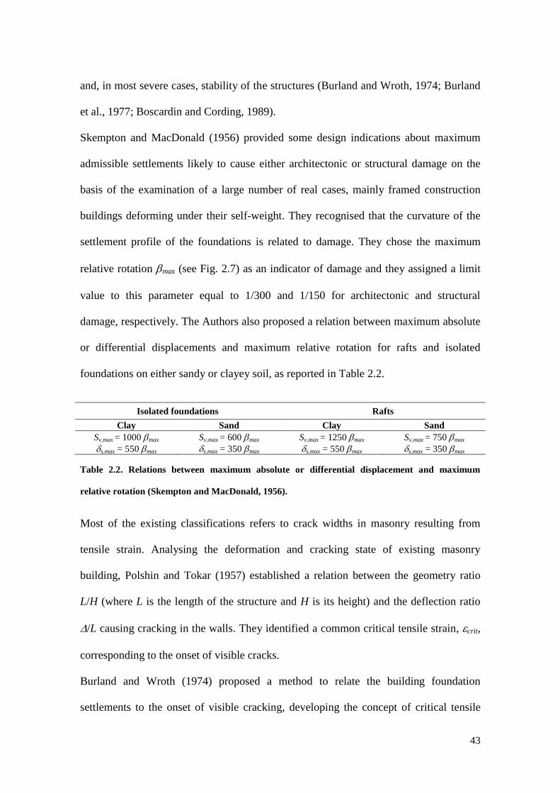
43

and, in most severe cases, stability of the structures (Burland and Wroth, 1974; Burland

et al., 1977; Boscardin and Cording, 1989).

Skempton and MacDonald (1956) provided some design indications about maximum

admissible settlements likely to cause either architectonic or structural damage on the

basis of the examination of a large number of real cases, mainly framed construction

buildings deforming under their self-weight. They recognised that the curvature of the

settlement profile of the foundations is related to damage. They chose the maximum

relative rotation max (see Fig. 2.7) as an indicator of damage and they assigned a limit

value to this parameter equal to 1/300 and 1/150 for architectonic and structural

damage, respectively. The Authors also proposed a relation between maximum absolute

or differential displacements and maximum relative rotation for rafts and isolated

foundations on either sandy or clayey soil, as reported in Table 2.2.

Isolated foundations Rafts

Clay Sand Clay Sand

Sv,max = 1000 max Sv,max = 600 max Sv,max = 1250 max Sv,max = 750 max

s,max = 550 max s,max = 350 max s,max = 550 max s,max = 350 max

Table 2.2. Relations between maximum absolute or differential displacement and maximum

relative rotation (Skempton and MacDonald, 1956).

Most of the existing classifications refers to crack widths in masonry resulting from

tensile strain. Analysing the deformation and cracking state of existing masonry

building, Polshin and Tokar (1957) established a relation between the geometry ratio

L/H (where L is the length of the structure and H is its height) and the deflection ratio

/L causing cracking in the walls. They identified a common critical tensile strain, crit,

corresponding to the onset of visible cracks.

Burland and Wroth (1974) proposed a method to relate the building foundation

settlements to the onset of visible cracking, developing the concept of critical tensile

44

strain (Polshin and Tokar, 1957). In particular, they investigated the relation between

the maximum deflection ratio (/L)max and the maximum tensile strain occurring in a

building idealised as an isotropic, linear-elastic deep beam (Timoshenko, 1955)

subjected to either pure bending or pure shear deformation. In pure bending the

maximum tensile strain b,max is horizontal, while in shear it is indicated as d,max and it

is oriented at 45° (the subscript d stands for diagonal). For such specified deformation

modes, the relation between the maximum deflection ratio (/L)max and the maximum

tensile strain is described by the following equations:

2

181

12b,max

L EJ

L y L HG

(2.22)

2

118

d ,max

L HG

L EJ

(2.23)

where y is the distance of the neutral axis, whose position is assumed either at the base

or at mid-height of the beam, from the bottom; L and H are the length and the height of

the beam, respectively; J is the second moment of area of the beam; E and G are the

Young’s and shear stiffness moduli, respectively.

The Authors also highlighted, however, that the ratio E/G for a real structure can be

very different from that calculated by assuming an isotropic behaviour as for the beam.

Burland et al. (1977) introduced a classification with six categories of increasing

damage, which is based on the ease of repair and also provides several indications on

the likely width and number of cracks associated to each category. Such classification is

reported in Table 2.3: categories from 0 to 2 are essentially associated to aesthetic

45

damage, category 3 to the attainment of some serviceability limit state for the structure,

while in categories 4 and 5 the structure reaches an ultimate limit state.

This classification was developed to provide a guide for standard domestic and office

buildings in brickwork or blockwork and stone masonry. Although widely adopted in

the geotechnical engineering practice, its applicability to monumental and historical

structures may be questionable (Viggiani and Soccodato, 2004).

In an important development, Boscardin and Cording (1989) replaced the concept of

critical tensile strain with that of limiting tensile strain, lim. They analysed case

histories of a number of brick-bearing-wall and framed buildings affected by excavation

with regard to the limiting tensile strain.

The Authors, in particular, overcame the model presented by Burland and Wroth (1974)

adding the effect of horizontal strains h on the onset of visible cracking. Assuming

homogeneous horizontal straining across the whole beam, it is possible to superimpose

h to b,max or d,max, separating bending and shear deformation modes. The resultant

strains are expressed as in the following equations:

b,r b,max h

(2.24)

2

2 21 1

2 2d ,r h h d ,max

(2.25)

Based on the data collected by Boscardin and Cording (1989), Burland (1995) proposed

that the attainment of each category of damage might be broadly related to characteristic

values of the limiting tensile strain, as reported in Table 2.4. The Author integrated the

previous classification of Burland et al. (1977) and defined damage charts of deflection

ratio /L versus horizontal strain h, as shown in the example of Figure 2.9.

46

Category of damage Normal degree of severity Description of typical damage

(easy of repair in italic type)

0 Negligible Hairline cracks less than about 0.1mm

1 Very slight

Fine cracks which are easily treated during

normal decoration. Damage generally restricted

to internal wall finishes. Close inspection may

reveal some cracks in external brickworks or

masonry. Typical crack widths up to 1mm.

2 Slight

Cracks easily filled. Re-decoration probably

required. Recurrent cracks can be masked by

suitable linings. Cracks may be visible

externally and some repointing may be required

to ensure weather-tightness. Doors and

windows may stick slightly. Typical crack

width up to 5mm.

3 Moderate

The cracks require some opening up and can be

patched by mason. Repointing of external

brickwork and possibly a small amount of

brickwork to be replaced. Doors and windows

sticking. Service pipes may fracture. Weather-

tightness often impaired. Typical crack widths

are 5÷15mm or several up to 3mm.

4 Severe

Extensive repair work involving breaking-out

and replacing sections of walls, especially over

doors and windows. Windows and door frames

distorted, floor sloping noticeably. Walls

leaning or bulging noticeably, some loss of

bearing in beams. Service pipes disrupted.

Typical crack widths are 15÷25mm but also

depends on the number of cracks.

5 Very severe

This requires a major repair job involving

partial or complete rebuilding. Beams lose

bearing, walls lean badly and require shoring.

Windows broken with distortion. Danger of

instability. Typical crack widths are greater

than 25mm but depends on the number of

cracks.

Table 2.3. Damage classification (Burland et al., 1977).

Category of damage Normal degree of severity Limiting tensile strain (%)

0 Negligible 0÷0.05

1 Very slight 0.05÷0.075

2 Slight 0.075÷0.15

3 Moderate 0.15÷0.3

4 and 5 Severe to Very severe >0.3

Table 2.4. Damage category and limiting tensile strain (Boscardin and Cording, 1989; Burland,

1995).

47

Figure 2.9. Burland’s damage classification.

2.4.2 Methodological approach to damage evaluation

Mair et al. (1996) described the assessment procedure of building damage induced by

settlements that was firstly applied on the Jubilee Line Extension (JLE) of London.

The methodology consists of three phases (Mair et al., 1996) which are referred to

“preliminary assessment” (Phase 1), “second phase assessment” (Phase 2) and “detailed

evaluation” (Phase 3).

In Phase 1 the presence of buildings is not considered and the free-field settlement

profiles are calculated by empirical expressions. Maximum absolute settlement and

rotation are calculated in correspondence with the area of the building and, if these

values are lower than 10 mm and 1/500 respectively, no further action is required,

otherwise a Phase 2 assessment has to be carried out. This indication is obviously

conservative, because the stiffness of the neglected surface structure, in general, tends to

reduce the differential displacements, as previously discussed.

In Phase 2 free-field horizontal and vertical displacements are calculated for each

building individually. Each structure is assumed to follow the ground movements and it

48

is represented as an elastic beam, described by its length L, its height H and the ratio of

Young’s modulus over the shear stiffness modulus E/G (Burland and Wroth, 1974).

The deflection ratio and the average horizontal strain along the building are evaluated

and in this approach the zones of hogging (i.e. tension) and sagging (i.e. compression)

are treated independently. In particular, the deflection ratio and the average horizontal

strain are calculated for each hogging and/or sagging zone of the building; these can be

related to categories of potential damage (Table 2.4). Alternatively, the category of

damage can be obtained by calculating the tensile strain developing in the building as

outlined by Mair et al. (1996). For damage categories of 2 (Slight) or smaller, only

aesthetic damage is predicted and, thus, no further analysis is required, while for

buildings with a potential damage category of 3 (Moderate) or higher a detailed

evaluation is required.

Although the Phase 2 calculation is more detailed than the preliminary assessment, it is

conservative since the building is assumed to follow the free-field settlement trough (i.e.

its stiffness is completely neglected).

In Phase 3 more details of the building and of the tunnel construction are taken into

account. This includes the orientation of the building with respect to the tunnel, building

features such as the foundation design and structural continuity and their effect on the

soil-structure interaction. Mair et al. (1996) pointed out that, due to the conservative

assumptions of the second phase assessment, the detailed evaluation will usually predict

lower categories of damage than obtained from the previous phase. However, if the risk

remains high (i.e. damage category of 3 or higher), protective measures have to be

considered, when necessary.

A new generic approach to the second stage of the assessment of the potential building

damage was developed by Harris and Franzius (2005). Such methodology aims at

49

improving the effectiveness and efficiency of the process whilst maintaining

consistency with Phase 3 of the method outlined by Mair et al. (1996). The ambition is

to reduce the effort expended in producing a large number of Phase 2 calculations for

individual buildings which show, in most cases, that the potential damage is within

acceptable limits. The Authors discussed about the inefficiency of the Phase 3 approach

to settlement assessment on the base of a specific experience (i.e. the Jubilee Line

Extension Contract 102 in London): for many of the Phase 2 assessments undertaken, a

low damage category is evident a priori and, consequently, a detailed evaluation for all

buildings is not justified. The proposal for generic Phase 2 assessments is to apply the

same assumptions and calculation methods as used previously for the assessment of

individual buildings, but applying these only to representative sections taken through

the surface settlement profiles determined in the Phase 1 assessment. Along each

section, a high number of different building geometries are analysed and the worst case,

i.e. the maximum tensile strain, for any building geometry located along the section is

then determined. This approach avoids the production of hundreds or thousands of

Phase 2 calculations for individual buildings, it gives improved insight into the variation

of maximum tensile strain along the route alignment and it identifies potentially

problematic areas to be more efficiently targeted for further assessment.

This generic method, however, cannot take into account of varying foundation depths

due to the fact that it is based on surface settlement contours.

50

3. Tunnelling-induced settlements in coarse-grained soils: the case of

the new Milan metro-line 5

3.1 Purpose of Chapter 3

This chapter proposes a detailed analysis of the displacement field induced by

tunnelling activities in granular soils, taking as reference the case study of the new

metro-line 5 of Milan (Italy). The two twin tunnels of the line were recently constructed

in sand and gravel, partially below the water table, with earth pressure balance (EPB)

machines to safely perform the excavation and to minimise the surface subsidence.

Measurements of tunnelling-induced settlements collected during the construction of the

line 5 are discussed and interpreted. The attention is firstly given to the monitoring data

recorded under free-field conditions (i.e. no structures on the ground surface) during and

after the construction of the first and the second tunnel. Settlement data are

back-analysed using the classical empirical predictions, both in the transversal and

longitudinal directions, providing an exhaustive description of the EPB tunnelling effect

under this specific geotechnical conditions.

Then, the influence of different excavation parameters (such as face pressure, grouting

pressure, machine thrust, etc.) on the subsidence due to the construction of the first and

the second tunnel of the metro-line is also investigated in detail.

Finally, measurements of the vertical displacements observed in correspondence with a

9-storey reinforced concrete building in interaction with the metro-line are analysed,

providing specific information on the evolution of the surface structure response during

tunnelling.

51

3.2 Tunnel construction

The twin tunnels of the metro-line 5 recently constructed in Milan (Italy) run from north

to west of the city with a total length of 12.6 km and 19 access stations (Fig. 3.1)

(Fargnoli et al., 2013).

The portions of the metro-line considered in this study extend for about 1.3 km between

San Siro and Segesta stations and for a length of about 600 m between Lotto and

Portello stations (Fig. 3.1).

Figure 3.1. Metro-line 5 of Milan (the reference segments of the route between the stations of

San Siro-Segesta and Lotto-Portello are underlined by the green and red circles, respectively).

The tunnels, partially excavated under the water table, have a separation between the

two axes, d, of about 15 m and a mean depth z0 = 15 m. This latter reaches its maximum

value of about 23 m at Lotto station.

In order to effectively minimise ground movements in these highly-populated areas,

EPB machines were selected.

The EPB machine makes use of a rotating cutter-head as a tool of excavation; the

excavated material, kept under pressure in the bulk chamber, ensures face stability and

52

it limits surface settlements. Face pressure is generally set as a function of the total

horizontal lithostatic pressure at rest acting at the depth of the tunnel.

In this case study the EPB shields have a total length of about 10 m and a thickness of

30 mm. They are characterised by an outer diameter of 6.69 m at the face and an inner

one of 6.67 m at the tail. The maximum excavation diameter at the face can be increased

up to 6.71 m. Six pressure cells are located on each EPB face as shown in Figure 3.2.

Figure 3.2. Location of the pressure cells on the EPB face.

A total thrust of about 50500 kN is required for the advancement of each machine. It is

provided by 38 hydraulic jacks located on the perimeter of the shield body, acting on

the already cast in place lining.

The tunnel lining, set in place inside the shield tail to support the tunnel as the machine

advances, consists in concrete cast-in-place rings characterised by a length of 1.4 m and

a thickness of 30 cm. The outer and inner diameters of the lining ring are equal to

6.40 m and 5.80 m, respectively. The external diameter of the final lining is always

smaller than the excavated one, in order to allow the advancement of the machine and of

the shield.

The gap created behind the lining segments after their erection is promptly filled in

order to minimise the settlement. A two-component back-filling grouting, consisting in

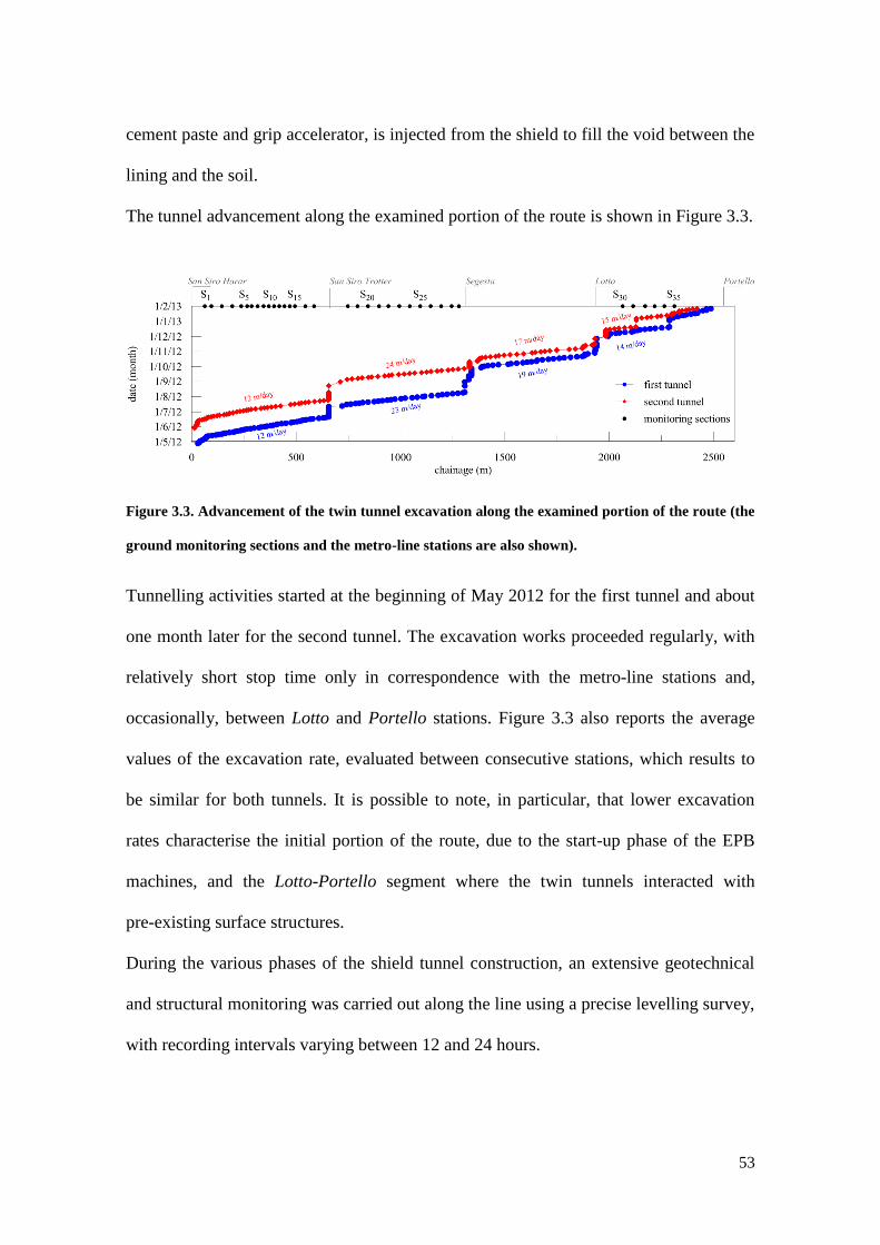
53

cement paste and grip accelerator, is injected from the shield to fill the void between the

lining and the soil.

The tunnel advancement along the examined portion of the route is shown in Figure 3.3.

Figure 3.3. Advancement of the twin tunnel excavation along the examined portion of the route (the

ground monitoring sections and the metro-line stations are also shown).

Tunnelling activities started at the beginning of May 2012 for the first tunnel and about

one month later for the second tunnel. The excavation works proceeded regularly, with

relatively short stop time only in correspondence with the metro-line stations and,

occasionally, between Lotto and Portello stations. Figure 3.3 also reports the average

values of the excavation rate, evaluated between consecutive stations, which results to

be similar for both tunnels. It is possible to note, in particular, that lower excavation

rates characterise the initial portion of the route, due to the start-up phase of the EPB

machines, and the Lotto-Portello segment where the twin tunnels interacted with

pre-existing surface structures.

During the various phases of the shield tunnel construction, an extensive geotechnical

and structural monitoring was carried out along the line using a precise levelling survey,

with recording intervals varying between 12 and 24 hours.

54

3.3 Ground conditions and geotechnical characterisation

The city of Milan is located in northern Italy, in the central part of the Padana plain, and

it rests on a deep glacial and alluvial Pleistocene formation. The upper part of this

deposit mainly consists of sand and gravel, with a percentage of silt increasing with

depth. A formation of conglomerate and sandstone underlies this upper deposit, while

sand and clay are present at greater depth. The new metro-line is located within the

granular unit of the upper formation, mainly consisting of gravel and sand of

fluvioglacial and alluvial origin.

Along the metro-line an extensive geotechnical investigation was carried out at the

design stage of the work, as summarised in Table 3.1.

Granulometric analyses were conducted on the disturbed samples taken from the core

drillings.

investigation reference portion of the route

San Siro-Segesta Lotto-Portello

core drillings instrumented with

open pipe piezometers

3 boreholes (CD1, CD2 and CD3)

to a depth of 21-27 m from the

ground surface

2 boreholes (CD4 and CD5) to a

depth of 24-30 m from the

ground surface

SPT tests 13 tests conducted in CD1, 11 in

CD2 and 11 in CD3

14 tests conducted in CD4 and 12

ones in CD5

constant-head Lenfranc-type

permeability tests

2 tests in CD1, 1 test in CD2 and 1

test in CD3 2 tests in CD4 and 1 test in CD5

disturbed samples taken from

the core drillings

19 samples 14 samples

Table 3.1. Details of the geotechnical investigation carried out along the reference portions of the

route.

The soil stratigraphy at the reference sites is shown in Figure 3.4 together with the

hydrostatic water level, measured with open pipe piezometers and detected on average

at 15 m below the ground surface. The gravelly-sand soil results as the main component

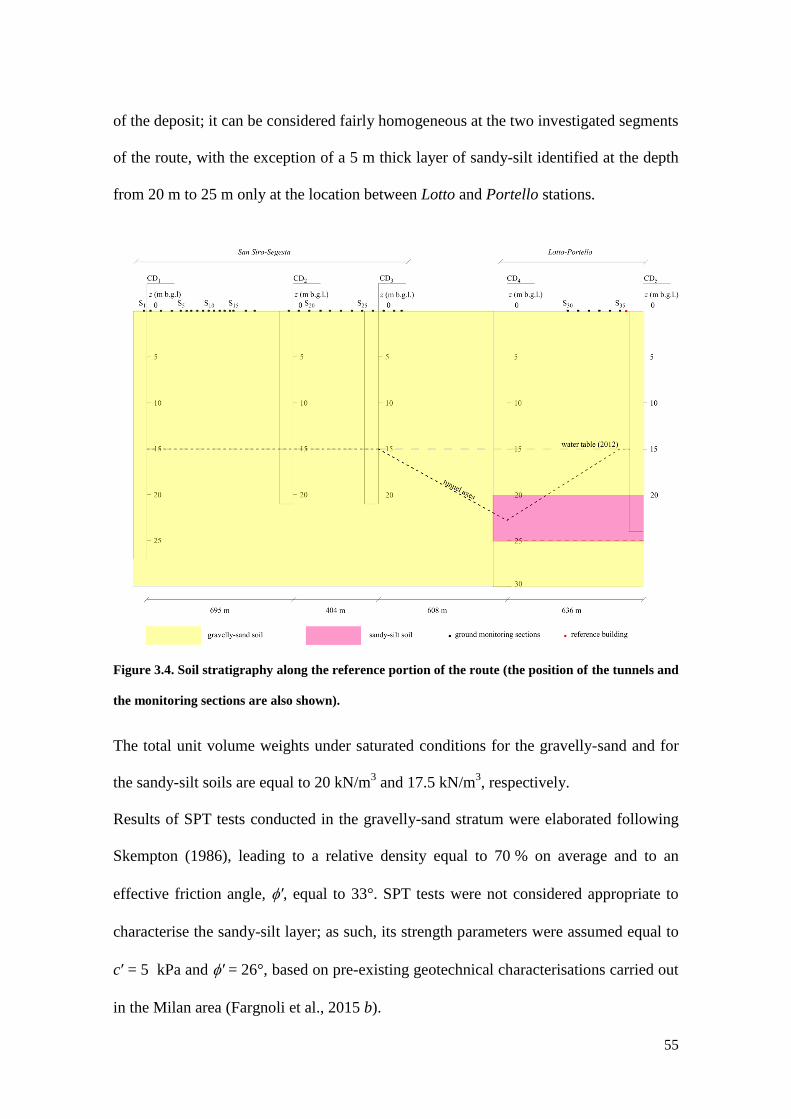
55

of the deposit; it can be considered fairly homogeneous at the two investigated segments

of the route, with the exception of a 5 m thick layer of sandy-silt identified at the depth

from 20 m to 25 m only at the location between Lotto and Portello stations.

Figure 3.4. Soil stratigraphy along the reference portion of the route (the position of the tunnels and

the monitoring sections are also shown).

The total unit volume weights under saturated conditions for the gravelly-sand and for

the sandy-silt soils are equal to 20 kN/m3 and 17.5 kN/m

3, respectively.

Results of SPT tests conducted in the gravelly-sand stratum were elaborated following

Skempton (1986), leading to a relative density equal to 70 % on average and to an

effective friction angle, ′, equal to 33°. SPT tests were not considered appropriate to

characterise the sandy-silt layer; as such, its strength parameters were assumed equal to

c′ = 5 kPa and ′ = 26°, based on pre-existing geotechnical characterisations carried out

in the Milan area (Fargnoli et al., 2015 b).

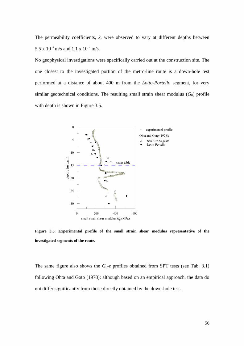
56

The permeability coefficients, k, were observed to vary at different depths between

5.5 x 10-3

m/s and 1.1 x 10-2

m/s.

No geophysical investigations were specifically carried out at the construction site. The

one closest to the investigated portion of the metro-line route is a down-hole test

performed at a distance of about 400 m from the Lotto-Portello segment, for very

similar geotechnical conditions. The resulting small strain shear modulus (G0) profile

with depth is shown in Figure 3.5.

Figure 3.5. Experimental profile of the small strain shear modulus representative of the

investigated segments of the route.

The same figure also shows the G0-z profiles obtained from SPT tests (see Tab. 3.1)

following Ohta and Goto (1978): although based on an empirical approach, the data do

not differ significantly from those directly obtained by the down-hole test.

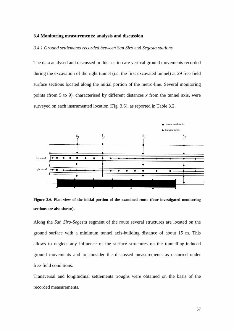
57

3.4 Monitoring measurements: analysis and discussion

3.4.1 Ground settlements recorded between San Siro and Segesta stations

The data analysed and discussed in this section are vertical ground movements recorded

during the excavation of the right tunnel (i.e. the first excavated tunnel) at 29 free-field

surface sections located along the initial portion of the metro-line. Several monitoring

points (from 5 to 9), characterised by different distances x from the tunnel axis, were

surveyed on each instrumented location (Fig. 3.6), as reported in Table 3.2.

Figure 3.6. Plan view of the initial portion of the examined route (four investigated monitoring

sections are also shown).

Along the San Siro-Segesta segment of the route several structures are located on the

ground surface with a minimum tunnel axis-building distance of about 15 m. This

allows to neglect any influence of the surface structures on the tunnelling-induced

ground movements and to consider the discussed measurements as occurred under

free-field conditions.

Transversal and longitudinal settlements troughs were obtained on the basis of the

recorded measurements.

58

Monitoring sections

S1 number 10006 10005 10004 10003 10002 10001 x (m) -32.3 -22.1 -15.4 -8.0 -0.1 6.6

S2 number 10012 10011 10010 10009 10008 10007 x (m) -32.7 -21.5 -15.3 -8.2 -0.3 6.5

S3 number 10018 10017 10016 10015 10014 10013 x (m) -31.8 -21.3 -15.3 -7.6 0.0 5.9

S4 number 10025 10024 10023 10022 10021 10020 10019 x (m) -31.7 -21.9 -15.3 -7.0 0.0 6.5 13.9

S5 number 10032 10031 10030 10029 10028 10027 10026

x (m) -30.4 -21.4 -14.7 -7.3 0.0 6.9 14.6

S6 number 10039 10038 10037 10036 10035 10034 10033

x (m) -31.5 -21.5 -15.3 -7.6 0.0 6.5 16.2

S7 number 10046 10045 10044 10043 10042 10041 10040

x (m) -31.3 -21.6 -15.3 -7.5 0.0 7.0 15.9

S8 number 10051 10050 10049 10048 10047 x (m) -21.6 -15.3 -7.7 0.2 6.6

S9 number 10056 10055 10054 10053 10052 x (m) -21.5 -15.3 -7.8 0.0 6.6

S10 number 10061 10060 10059 10058 10057 x (m) -21.8 -15.2 -7.9 0.0 6.5

S11 number 10066 10065 10064 10063 10062

x (m) -21.9 -15.3 -7.9 0.0 6.6

S12 number 10071 10070 10069 10068 10067

x (m) -21.9 -15.2 -7.7 0.0 6.6

S13 number 10076 10075 10074 10073 10072

x (m) -22.0 -15.3 -7.7 0.0 6.5

S14 number 10081 10080 10079 10078 10077 x (m) -21.4 -15.2 -7.7 0.0 6.6

S15 number 10086 10085 10084 10083 10082 x (m) -19.4 -15.2 -7.6 0.0 6.4

S16

number 10092 10091 10090 10089 10088 10087 x (m) -21.2 -15.2 -7.6 0.0 6.5 16.1

S17 number 10098 10097 10096 10095 10094 10093

x (m) -21.5 -15.3 -8.1 -0.4 5.3 15.9

S18 number 20006 20005 20004 20003 20002 20001

x (m) -31.3 -21.7 -13.6 -7.5 0.0 5.9

S19 number 20011 20010 20009 20008 20007

x (m) -21.6 -14.0 -7.7 0.0 6.8

S20 number 20016 20015 20014 20013 20012 x (m) -21.6 -14.3 -7.7 0.0 6.5

S21 number 20023 20022 20021 20020 20019 20018 20017 x (m) -33.5 -22.1 -16.1 -8.3 0.0 5.7 16.7

S22 number 20030 20029 20028 20027 20026 20025 20024 x (m) -29.1 -21.7 -14.9 -7.7 0.0 5.1 15.5

S23 number 20035 20034 20033 20032 20031

x (m) -21.5 -14.2 -6.4 0.0 6.4

S24 number 20040 20039 20038 20037 20036

x (m) -21.1 -14.2 -7.6 0.0 6.3

S25 number 20045 20044 20043 20042 20041

x (m) -21.8 -13.9 -7.6 0.0 6.7

S26 number 20050 20049 20048 20047 20046 x (m) -21.0 -14.2 -7.7 0.0 6.1

S27 number 20055 20054 20053 20052 20051 x (m) -21.1 -15.2 -6.4 0.0 6.8

S28 number 20060 20059 20058 20057 20056 x (m) -14.3 -5.6 0.0 6.1 14.6

S29 number 20069 20068 20067 20066 20065 20064 20063 20062 20061

x (m) -40.4 -31.4 -20.0 -14.7 -7.2 0.0 5.6 17.4 27.1

Table 3.2. Monitoring benchmarks on the instrumented sections between San Siro-Segesta stations.

59

Surface settlement profiles evolve with the excavation advancement. Figure 3.7 shows

their final configuration as recorded at each of the 29 monitoring sections at steady-state

conditions, i.e. for a sufficiently large distance between the section and the tunnel face.

In each monitoring section the maximum settlement, Sv,max(I)

, varying in the range

6.0-21.4 mm, is observed at the tunnel centre line (x = 0) and gradually decreases

moving away from it, as expected in the case of a single tunnel excavation.

These measurements were fitted by a Gaussian distribution curve (Eq. 2.1 of Chap. 2;

Peck, 1969), using K values appropriate to coarse-grained soils (0.25-0.45; Mair and

Taylor, 1997; Puzrin et al, 2012). In this way, it was possible to evaluate for each

location the corresponding volume loss, VL(I)

(%), as shown in the example of Figure

3.8, referring to the section S7. The tunnelling influence zone extends symmetrically for

about 15-20 m from the tunnel axis.

Figure 3.7. Settlements measured at ground surface after the first tunnel construction.

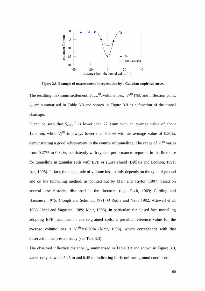
60

Figure 3.8. Example of measurement interpretation by a Gaussian empirical curve.

The resulting maximum settlement, Sv,max(I)

, volume loss, VL(I)

(%), and inflection point,

ix, are summarised in Table 3.3 and shown in Figure 3.9 as a function of the tunnel

chainage.

It can be seen that Sv,max(I)

is lower than 22.0 mm with an average value of about

12.0 mm, while VL(I)

is always lower than 0.90% with an average value of 0.50%,

demonstrating a good achievement in the control of tunnelling. The range of VL(I)

varies

from 0.27% to 0.82%, consistently with typical performances reported in the literature

for tunnelling in granular soils with EPB or slurry shield (Leblais and Bochon, 1991;

Ata, 1996). In fact, the magnitude of volume loss mainly depends on the type of ground

and on the tunnelling method, as pointed out by Mair and Taylor (1997) based on

several case histories discussed in the literature (e.g.: Peck, 1969; Cording and

Hansmire, 1975; Clough and Schmidt, 1981; O’Reilly and New, 1982; Attewell et al.

1986; Uriel and Sagaseta, 1989; Mair, 1996). In particular, for closed face tunnelling

adopting EPB machines in coarse-grained soils, a possible reference value for the

average volume loss is VL(I)

= 0.50% (Mair, 1996), which corresponds with that

observed in the present study (see Tab. 3.3).

The observed inflection distance ix, summarised in Table 3.3 and shown in Figure 3.9,

varies only between 5.25 m and 6.45 m, indicating fairly uniform ground conditions.

61

Monitoring sections Sv,max (I)

(mm) VL (I)

(%) ix (m)

S1 7.5 0.33 6.00

S2 7.7 0.33 6.00

S3 8.4 0.37 6.00

S4 14.2 0.58 5.55

S5 20.4 0.80 5.25

S6 9.3 0.38 5.70

S7 14.8 0.56 5.25

S8 13.3 0.54 5.70

S9 11.8 0.45 5.25

S10 11.3 0.42 5.25

S11 12.6 0.47 5.25

S12 10.1 0.41 5.55

S13 17.7 0.70 5.55

S14 17.3 0.67 5.40

S15 12.2 0.46 5.25

S16 8.8 0.40 6.45

S17 11.4 0.50 6.00

S18 10.2 0.44 6.00

S19 10.1 0.39 5.25

S20 10.6 0.41 5.25

S21 10.8 0.48 6.00

S22 6.0 0.27 6.00

S23 9.4 0.36 5.25

S24 9.6 0.39 5.55

S25 13.1 0.50 5.25

S26 13.4 0.54 5.55

S27 21.4 0.82 5.25

S28 16.0 0.70 6.00

S29 18.9 0.82 6.00

average value 12.4 0.50 5.60

Table 3.3. Values of Sv,max (I)

, VL(I)

(%) and ix at the monitoring sections between San Siro and

Segesta stations.

62

Figure 3.9. Values of Sv,max (I)

(a), VL(I)

(b) and ix (c) at the examined monitoring sections along the

initial portion of the metro-line route.

A vast majority of the settlements measured at the ground surface falls in the range

delimited by the Gaussian empirical predictions for K values equal to 0.25 (upper

bound) and 0.45 (lower bound), as shown in Figure 3.10 in terms of normalised

settlement curves. In particular, the figure shows that the Gaussian curve for K = 0.35

(i.e. ix = 5.25 m) nicely fits the measurements within a horizontal distance of x = ±2ix,

while data recorded at larger distances are best-fitted by a Gaussian curve characterised

by K = 0.45. A similar pattern was also observed by Grant and Taylor (2000) in

63

centrifuge model tests. It indicates that the Gaussian distribution as obtained for

K = 0.35 may underestimate the magnitude of the settlements in the outer region of the

subsidence trough.

This experimental evidence can be more effectively highlighted by plotting the same set

of measurements in an alternative way, as illustrated in Figure 3.11. In this plot the

curves are linearised in such a way that the inverse of their gradient is the inflection

point, ix.

Figure 3.12 illustrates the comparison between measured settlements at selected

instrumented sections and the associated best empirical predictions as obtained for

different K values in the range 0.35-0.40. Despite the limited variability of ix (see Fig.

3.9 c), it is possible to observe from Figure 3.12 that the maximum settlement

magnitude increases as ix decreases, in accordance with Cording (1991).

Figure 3.10. Normalised settlements measured at ground surface and comparison with Gaussian

empirical curves.

64

Figure 3.11. Linearised settlements at ground surface.

Figure 3.12. Transversal settlement profiles: trough widths and settlement magnitudes (ix values for

each section are reported in Table 3.3).

A possible explanation of such a feature can be provided with reference to limit

conditions. In fact, several case-histories of tunnel failures in sand (Chambon and Corté,

1994) and in clay (Mair, 1979) shown that the corresponding mechanisms are markedly

different: in clays it propagates upwards and outwards from the tunnel invert, becoming

significantly wider than the tunnel diameter; in sands, failure involves a narrow

“chimney” mechanism propagating almost vertically from the tunnel up to the ground

surface. This latter mechanism was also observed in laboratory studies on tunnels in

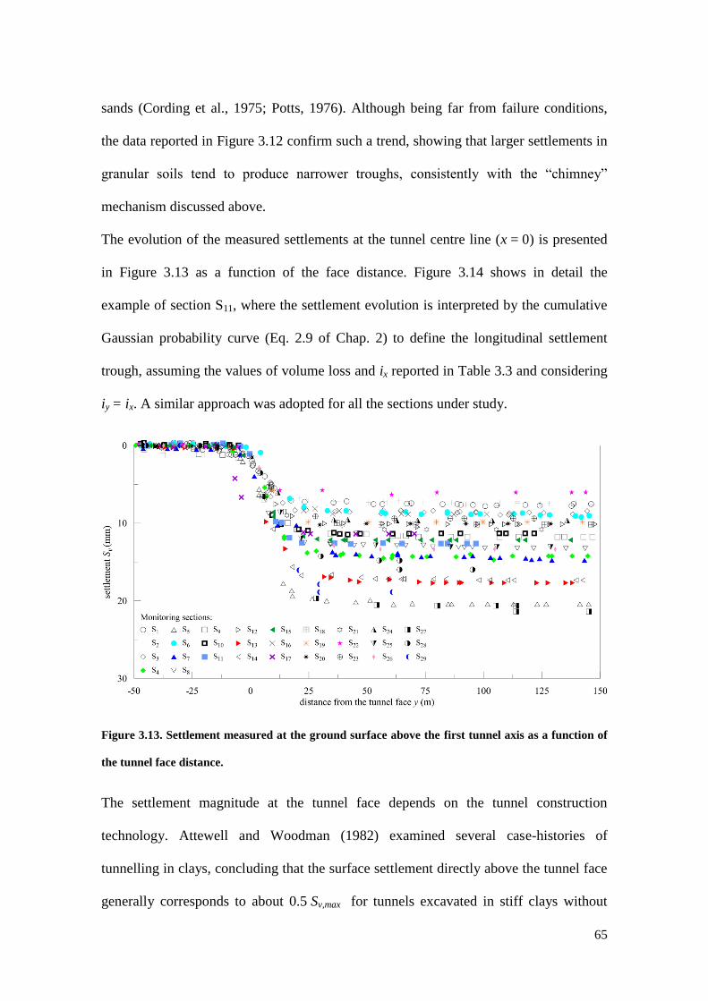
65

sands (Cording et al., 1975; Potts, 1976). Although being far from failure conditions,

the data reported in Figure 3.12 confirm such a trend, showing that larger settlements in

granular soils tend to produce narrower troughs, consistently with the “chimney”

mechanism discussed above.

The evolution of the measured settlements at the tunnel centre line (x = 0) is presented

in Figure 3.13 as a function of the face distance. Figure 3.14 shows in detail the

example of section S11, where the settlement evolution is interpreted by the cumulative

Gaussian probability curve (Eq. 2.9 of Chap. 2) to define the longitudinal settlement

trough, assuming the values of volume loss and ix reported in Table 3.3 and considering

iy = ix. A similar approach was adopted for all the sections under study.

Figure 3.13. Settlement measured at the ground surface above the first tunnel axis as a function of

the tunnel face distance.

The settlement magnitude at the tunnel face depends on the tunnel construction

technology. Attewell and Woodman (1982) examined several case-histories of

tunnelling in clays, concluding that the surface settlement directly above the tunnel face

generally corresponds to about 0.5 Sv,max for tunnels excavated in stiff clays without

66

face support, while showing values lower than 0.5 Sv,max for tunnels in soft clays with

face support provided by compressed air, as also reported in Mair and Taylor (1997).

Figure 3.14. Example of measurement interpretation by a cumulative Gaussian curve.

This is due to the fact that pressurised face tunnelling tends to limit ground movements

ahead of the tunnel face.

Field observations for shield tunnelling in loose silty-sand and soft clay (Moh et al.,

1996), in sands or silts (Nomoto et al., 1995) and in medium to dense sands overlain by

a clay layer (Ata, 1996), indicate that the major construction settlement is related to the

tail void, leading to surface settlement directly above the tunnel face generally much

lower than 0.5 Sv,max. This typically induces a horizontal translation of the Gaussian

cumulative curve (Mair and Taylor, 1997). This evidence is also supported by

centrifuge data (Imamura et al., 1998), irrespective of the ground condition (Sugiyama

et al., 1999).

Measurements of vertical displacements close (i.e. ± 1m) to the tunnel face, Sv,f (I)

, in

this segment of the route, were only available for 6 sections (i.e.: S1; S3; S7; S11; S18;

S20) out of the 29 ones examined. For those monitoring sections the surface settlements

at the tunnel face are in the range of 0.09-0.32 Sv,max(I)

, as summarised in Table 3.4,

indicating a satisfactory control of the face support during the excavation process.

67

Monitoring sections Sv,max(I)

(mm) Sv,f (I)

(mm) Sv,f (I)

/Sv,max(I)

S1 7.5 2.0 0.26

S3 8.4 2.7 0.32

S7 14.8 4.0 0.27

S11 12.6 1.1 0.09

S18 10.2 1.4 0.13

S20 10.6 1.5 0.14

Table 3.4. Maximum settlement Sv,max(I)

, tunnel face settlement Sv,f (I)

and Sv,f (I)

/Sv,max (I)

ratio at the

monitoring sections between San Siro and Segesta stations.

Figure 3.15 shows the original and translated cumulative curves for the 6 monitored

sections, the latter being obtained equating the empirical ratio Sv,f (I)

/Sv,max(I)

to the

measured one: the consistency between the longitudinal surface settlement trough and

the translated cumulative curve indicates that the main source of settlements is far from

the face, as suggested in the literature (Mair and Taylor, 1997; Ata, 1996; Imamura et

al., 1998; Sugiyama et al., 1999).

For all the other sections, where face settlement measurements were not available, the

corresponding translation ratio Sv,f (I)

/Sv,max(I)

was obtained by the settlement best-fitting

curve: its lowest value is equal to 0.02, an even lower value as compared to that

observed in the fully monitored 6 sections mentioned above.

Figure 3.16 illustrates all the available longitudinal data as plotted in terms of

normalised settlements, together with the best-fitting translated longitudinal troughs

obtained for sections S6 (Sv,f (I)

/Sv,max(I)

= 0.02) and S3 (Sv,f (I)

/Sv,max(I)

= 0.32). The figure

shows that a vast majority of data falls in the range delimited by these curves within a

distance from the face of y1 = -iy and y2 = 3.5iy (for iy = ix = 5.6 m, the average ix value

indicated in Fig. 3.11). However, the empirical profile is not able to accurately predict

the settlements occurring for y < y1, nor to capture the correct distance from the face at

which, for y > y2, steady-state conditions are achieved, this latter condition being

predicted at a shorter distance from the face than observed.

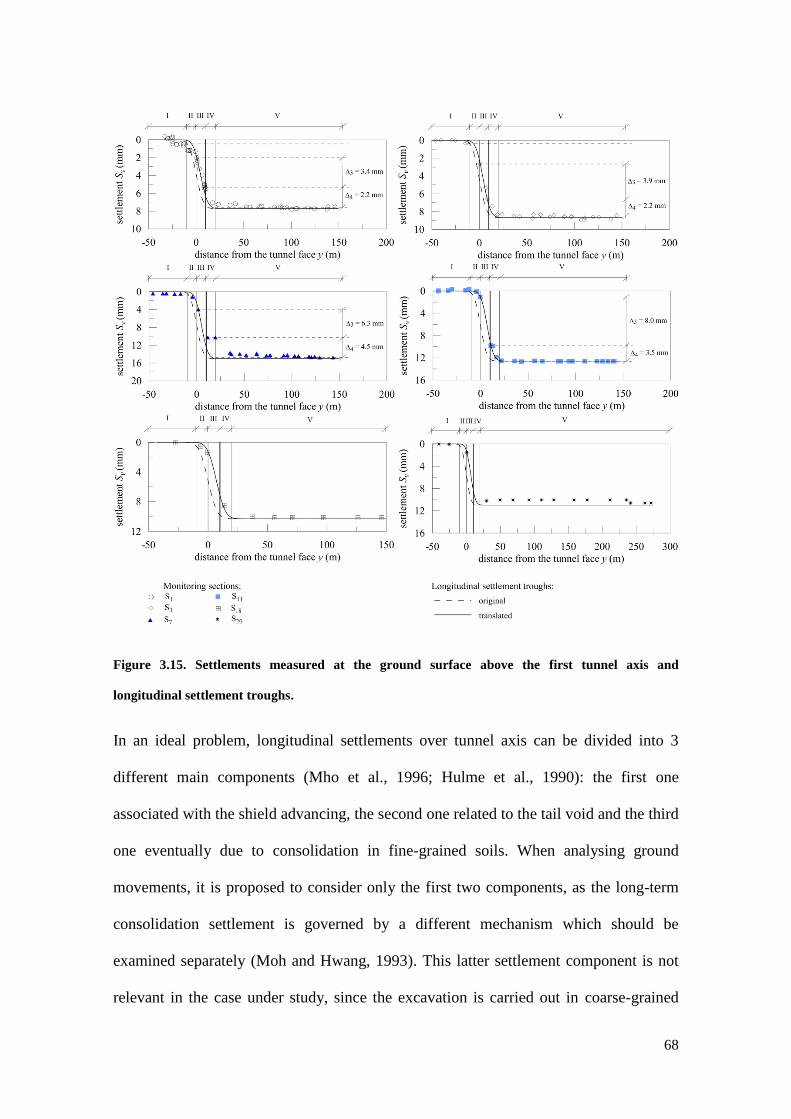
68

Figure 3.15. Settlements measured at the ground surface above the first tunnel axis and

longitudinal settlement troughs.

In an ideal problem, longitudinal settlements over tunnel axis can be divided into 3

different main components (Mho et al., 1996; Hulme et al., 1990): the first one

associated with the shield advancing, the second one related to the tail void and the third

one eventually due to consolidation in fine-grained soils. When analysing ground

movements, it is proposed to consider only the first two components, as the long-term

consolidation settlement is governed by a different mechanism which should be

examined separately (Moh and Hwang, 1993). This latter settlement component is not

relevant in the case under study, since the excavation is carried out in coarse-grained

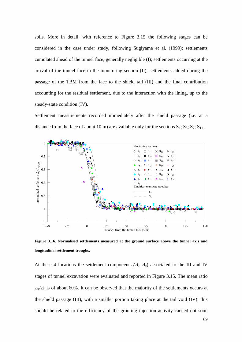
69

soils. More in detail, with reference to Figure 3.15 the following stages can be

considered in the case under study, following Sugiyama et al. (1999): settlements

cumulated ahead of the tunnel face, generally negligible (I); settlements occurring at the

arrival of the tunnel face in the monitoring section (II); settlements added during the

passage of the TBM from the face to the shield tail (III) and the final contribution

accounting for the residual settlement, due to the interaction with the lining, up to the

steady-state condition (IV).

Settlement measurements recorded immediately after the shield passage (i.e. at a

distance from the face of about 10 m) are available only for the sections S1; S3; S7; S11.

Figure 3.16. Normalised settlements measured at the ground surface above the tunnel axis and

longitudinal settlement troughs.

At these 4 locations the settlement components (3, 4) associated to the III and IV

stages of tunnel excavation were evaluated and reported in Figure 3.15. The mean ratio

4/3 is of about 60%. It can be observed that the majority of the settlements occurs at

the shield passage (III), with a smaller portion taking place at the tail void (IV): this

should be related to the efficiency of the grouting injection activity carried out soon

70

after the passage of the TBM to fill the tail void at the scope of minimising the ground

movements. This aspect is further discussed in the following.

3.4.2 Ground settlements recorded between Lotto and Portello stations

Transversal and longitudinal ground settlement profiles induced by the excavation of

the first tunnel along the Lotto-Portello segment of the metro-line (Fig. 3.17) are

represented in Figure 3.18 (a) and (b), respectively.

Figure 3.17. Plan view of the Lotto-Portello segment of the Milan metro-line 5.

Transversal profiles, in particular, refer to fully developed settlements achieved when

the first tunnel face was at a sufficient distance from the monitoring sections. The

maximum settlement Sv,max (I)

is generally very low and never exceeds 7 mm.

Along this portion of the route too, the transversal settlement troughs result to be

sufficiently well fitted by a Gaussian distribution curve with K values in the range

0.40-0.45, with the exception of the leftmost points of each section, whose values are

under-predicted by the empirical relation (Fig. 3.19); this is probably due to the

influence of nearby surface structures located along this segment (see Fig. 3.17).

71

The above interpolation allowed to back-evaluate the corresponding volume loss,

VL (I)

(%), which varies from 0.30% to 0.38% with an average value equal to 0.33%,

indicating, along this portion of the metro-line too, a well-performing EPB excavation

(e.g. Ata, 1996; Leblais and Bochon, 1991; Mair, 1996; Mair and Taylor, 1997).

Figure 3.18. Settlement measurements at ground sections in transversal (a) and longitudinal (b)

directions.

The values of maximum settlement Sv,max (I)

, K parameter and volume loss VL (I)

for all

the considered sections (i.e. from S30 to S35) are summarised in Table 3.5. The table also

reports the different depth of the tunnel axis, z0, at each location and the recording date

of the analysed settlement measurements.

Settlements surveyed at section S35 located near a multi-storey reinforced concrete

building undercrossed by the first tunnel of the metro-line was investigated with special

accuracy.

72

Monitoring sections Sv,max(I)

(mm) K (-) VL (I)

(%) z0 (m) date

S30 5.6 0.45 0.38 20.0 16/12/2012

S31 5.2 0.42 0.30 19.0 18/12/2012

S32 6.0 0.45 0.37 18.0 20/12/2012

S33 5.5 0.42 0.30 17.0 08/01/2013

S34 6.5 0.40 0.31 16.0 10/01/2013

S35 5.5 0.45 0.34 15.0 15/01/2013

Table 3.5. Values of maximum settlement, K parameter, volume loss, axis depth and surveying date

at the reference monitoring sections.

Figure 3.19. Transversal settlement troughs: measurements and best-fitting Gaussian curves.

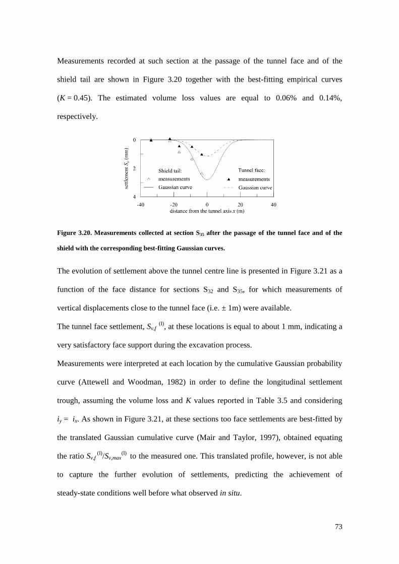
73

Measurements recorded at such section at the passage of the tunnel face and of the

shield tail are shown in Figure 3.20 together with the best-fitting empirical curves

(K = 0.45). The estimated volume loss values are equal to 0.06% and 0.14%,

respectively.

Figure 3.20. Measurements collected at section S35 after the passage of the tunnel face and of the

shield with the corresponding best-fitting Gaussian curves.

The evolution of settlement above the tunnel centre line is presented in Figure 3.21 as a

function of the face distance for sections S32 and S35, for which measurements of

vertical displacements close to the tunnel face (i.e. ± 1m) were available.

The tunnel face settlement, Sv,f (I)

, at these locations is equal to about 1 mm, indicating a

very satisfactory face support during the excavation process.

Measurements were interpreted at each location by the cumulative Gaussian probability

curve (Attewell and Woodman, 1982) in order to define the longitudinal settlement

trough, assuming the volume loss and K values reported in Table 3.5 and considering

iy = ix. As shown in Figure 3.21, at these sections too face settlements are best-fitted by

the translated Gaussian cumulative curve (Mair and Taylor, 1997), obtained equating

the ratio Sv,f (I)

/Sv,max(I)

to the measured one. This translated profile, however, is not able

to capture the further evolution of settlements, predicting the achievement of

steady-state conditions well before what observed in situ.

74

Figure 3.21. Settlements measured above the tunnel centre line at the monitoring sections S32 (a)

and S35 (b) with original and translated longitudinal profiles.

3.4.3 Effects induced on ground settlements by the excavation of the second metro-line

tunnel

Maximum settlements measured after the second excavation above the second tunnel

axis, Sv,max(II)

, are summarised in Table 3.6 for the 29 monitoring ground sections (from

S1 to S29) between San Siro and Segesta stations and for the 6 sections (from S30 to S35)

between Lotto and Portello stations. It varies from 8.0 mm to 27.8 mm with an average

value of about 12.0 mm.

The construction of the second tunnel produces an increase in settlement above the axis

of the first tunnel on average equal to 30%. The final vertical displacement recorded

above the first tunnel axis after the second excavation, identified as S′v,max(I)

and reported

in Table 3.6, ranges from 6.0 mm to 24.8 mm with an average value of about 15.0 mm.

75

Monitoring sections S'v,max(I)

(mm) Sv,max(II)

(mm) VL(TOT)

(%)

S1 10.0 11.0 0.88

S2 10.2 10.8 0.88

S3 11.1 12.3 0.99

S4 17.5 17.9 1.41

S5 23.1 8.0 1.19

S6 10.0 8.7 0.75

S7 16.2 9.5 0.98

S8 14.4 10.7 1.02

S9 13.5 13.7 1.03

S10 13.2 11.7 0.95

S11 14.6 10.7 0.96

S12 12.2 13.8 1.03

S13 20.5 27.8 1.89

S14 19.4 15.1 1.33

S15 14.2 11.6 0.97

S16 11.3 10.6 0.95

S17 15.1 11.0 1.06

S18 12.7 11.3 0.99

S19 12.6 9.6 0.84

S20 13.2 9.5 0.85

S21 13.3 9.3 0.94

S22 6.0 8.8 0.62

S23 12.4 10.1 0.85

S24 12.9 11.0 0.94

S25 16.6 12.7 1.10

S26 17.7 12.5 1.18

S27 24.8 15.7 1.51

S28 20.1 16.1 1.50

S29 23.8 19.7 1.81

S30 11.4 12.1 1.05

S31 10.3 11.9 1.00

S32 8.3 9.6 0.81

S33 8.2 8.4 0.74

S34 10.1 10.0 0.85

S35 8.7 9.2 0.84

Table 3.6. Values of final settlements and volume loss at the end of the second tunnel excavation.

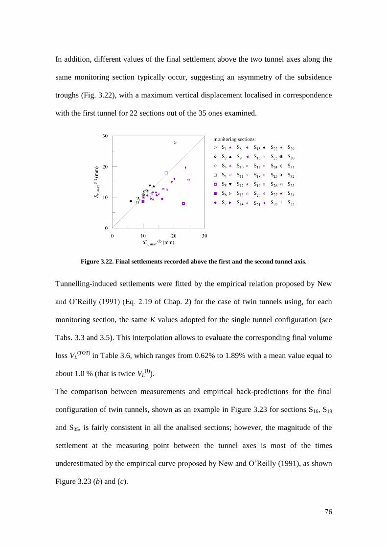
76

In addition, different values of the final settlement above the two tunnel axes along the

same monitoring section typically occur, suggesting an asymmetry of the subsidence

troughs (Fig. 3.22), with a maximum vertical displacement localised in correspondence

with the first tunnel for 22 sections out of the 35 ones examined.

Figure 3.22. Final settlements recorded above the first and the second tunnel axis.

Tunnelling-induced settlements were fitted by the empirical relation proposed by New

and O’Reilly (1991) (Eq. 2.19 of Chap. 2) for the case of twin tunnels using, for each

monitoring section, the same K values adopted for the single tunnel configuration (see

Tabs. 3.3 and 3.5). This interpolation allows to evaluate the corresponding final volume

loss VL(TOT)

in Table 3.6, which ranges from 0.62% to 1.89% with a mean value equal to

about 1.0 % (that is twice VL(I)

).

The comparison between measurements and empirical back-predictions for the final

configuration of twin tunnels, shown as an example in Figure 3.23 for sections S16, S19

and S35, is fairly consistent in all the analised sections; however, the magnitude of the

settlement at the measuring point between the tunnel axes is most of the times

underestimated by the empirical curve proposed by New and O’Reilly (1991), as shown

Figure 3.23 (b) and (c).

77

Figure 3.23. Interpretation of measurements by Gaussian empirical curves at monitoring sections

S16 (a), S19 (b) and S35 (c) (the reference K values are also reported in each plot).

The analysis carried out in the present study indicates that, in general, the sum of the

individual Gaussian curves for a single tunnel to predict the vertical movements above

twin tunnels, neglecting any interaction effect, may not give realistic settlement profiles

(Addenbrooke and Potts, 2001; Cooper et al., 2002; Chapman et al., 2007). This

78

procedure, in fact, does not take in account that the soil around the first tunnel has

already experienced a certain amount of stress relief and strain accumulation which is

very likely to reduce its initial stiffness.

This aspect becomes more evident when looking at the vertical displacements obtained

by subtracting the settlements measured after the first tunnel excavation from the final

values (Fig. 3.23). These data, which represent the settlements induced only by the

second excavation (Perez Saiz et al., 1981; Suwansawat and Einstein, 2007), are not

symmetric: in fact, the values on the left side of the axis of the second tunnel are well

interpreted by the empirical Gaussian curve proposed by Peck (1969) (Eq. 2.1 of Chap.

2,) which, conversely, underestimates the data on the right side.

As suggested in the literature (e.g. Chapman et al., 2007), the trough width parameter ix

could be increased for the second tunnel on the side nearest to the first tunnel in order to

take into account the interaction effects. For the investigated case, such a parameter was

increased in the region where x > -15 m (Fig. 3.23) using K values included in the range

0.42-0.70 to obtain a more adequate interpolation of the measurements. The above

evidence confirms that, also for this case-history, the presence of an existing tunnel

alters the expected pattern of vertical ground movements induced by a new excavation.

The evolution of the settlement profile with the excavation advancement along three

different transversal sections during the critical construction stages of the second tunnel

(i.e. the passage of the face and shield) is shown in Figure 3.24. At these locations the

components of settlement 2, 3 and 4, already defined in the previous Section 3.4.1,

were evaluated above the second tunnel.

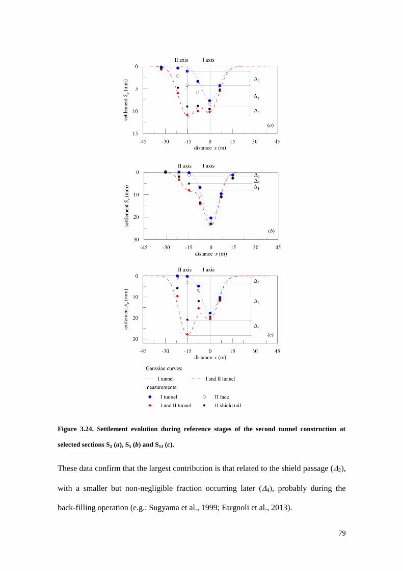
79

Figure 3.24. Settlement evolution during reference stages of the second tunnel construction at

selected sections S2 (a), S5 (b) and S13 (c).

These data confirm that the largest contribution is that related to the shield passage (,

with a smaller but non-negligible fraction occurring later (, probably during the

back-filling operation (e.g.: Sugyama et al., 1999; Fargnoli et al., 2013).

80

Figure 3.25. Interpretation of measurements above the second tunnel by original and translated

cumulative Gaussian curves at sections S2 (a), S5 (b) and S13 (c).

Figure 3.25 illustrates, with reference to the same sections (S2, S5 and S13), a

longitudinal representation of the settlements above the second tunnel axis together with

the original (Eq. 2.9 of Chap. 2; Attewell and Woodman, 1982) and translated (Mair

and Taylor, 1997) Gaussian cumulative curves.

81

The figure highlights that, also in these sections, the face settlements are best-fitted by

the translated Gaussian cumulative curve and it confirms the above discussed limits of

the empirical relation that predicts the attainment of final conditions too early with

respect to what indicated by in situ measurements.

3.4.4 Excavation parameters influencing ground settlements

EPB machine parameters were continuously monitored during the excavation works in

order to control tunnelling-induced subsidence.

In this section the effect of the following parameters on the ground settlements due to

the first tunnel excavation is firstly analysed: support pressure at the tunnel face

(Branque et al. 2002; Dimmock et al., 2002; Guedes de Melo and Santos Pereira, 2002;

Shirlaw et al., 2002; Suwansawat, 2002; Phienwej et al., 2006; Sirivachiraporn and

Phienwej, 2012); grouting pressure for the back-filling of the concrete lining (Peila et

al., 2011; Bilotta and Russo, 2012; Russo et al., 2012; Sirivachiraporn and Phienwej,

2012); machine stop time at monitored sections (Sirivachiraporn and Phienwej, 2012);

installation time for one-ring tunnel lining; machine thrust against the existing tunnel

lining to advance during the boring process (Branque et al., 2002; Dimmock et al.,

2002).

The excavation parameters are plotted in Figure 3.26, while their average values are

summarised in Table 3.7. In particular, Figure 3.26 (a) highlights that the face pressure

values applied along the initial portion of the route, on average equal to about 200 kPa,

are higher than the total horizontal stress acting at rest in correspondence with the tunnel

invert (i.e. 185 kPa) and this is probably due to the start-up phase of tunnelling. After

this stage, in fact, the values of the face support pressure were lower and, on average,

equal to 132 kPa. Figure 3.26 (b-e) shows a more regular trend of all the other

excavation parameters along the examined metro-line route.

82

Figure 3.26. Excavation parameters recorded during the first tunnel advancement.

83

As observed in the previous Section 3.4.1, most of the construction settlement is

associated to the shield passage. However, the ground movements induced by this

tunnelling stage cannot be controlled during the machine advancement (Sugiyama et al.,

1999).

In this study an attempt was first made to relate face settlements (available in a few

monitored sections) to face pressure, but in this respect no direct correlation could be

extracted from the few analysed monitoring data. However, all the data indicates that

face pressure clearly contributes in limiting the settlements at the tunnel face, as

previously discussed with reference to the values of the ratio Sv,f (I)

/Sv,max(I)

.

A second and more extended analysis, performed on all the 35 monitoring sections, was

carried out to explore the existence of possible correlations between the volume loss

VL (I) associated to the settlement Sv,max

(I) and the excavation parameters, as recorded

along a tunnel length of 8.4 m (that is six times the size of the tunnel lining ring, i.e.

4.2 m ahead and 4.2 m behind the monitored section).

Correlations are observed in the case of face and grouting pressures, as shown in

Figure 3.27 (a) and (b). In detail, the figure plots both the recorded data and their

average values, grouped according to eight classes of pressure defined in the interval

90-250 kPa. The data, although relatively dispersed, indicate a trend which proves the

role of face and grouting pressures in mitigating settlements and in reducing the related

volume loss. Grouting pressure plays a direct role in the settlement contribution 4,

which is related to the injection activity carried out soon after the passage of the TBM

to fill the tail void. As already discussed above, this contribution is small as compared

to that due to the shield passage, in contrast to what shown in Figure 3.27 (b) where an

evident reduction of the overall VL (I)

is observed for increasing values of grouting

pressure.

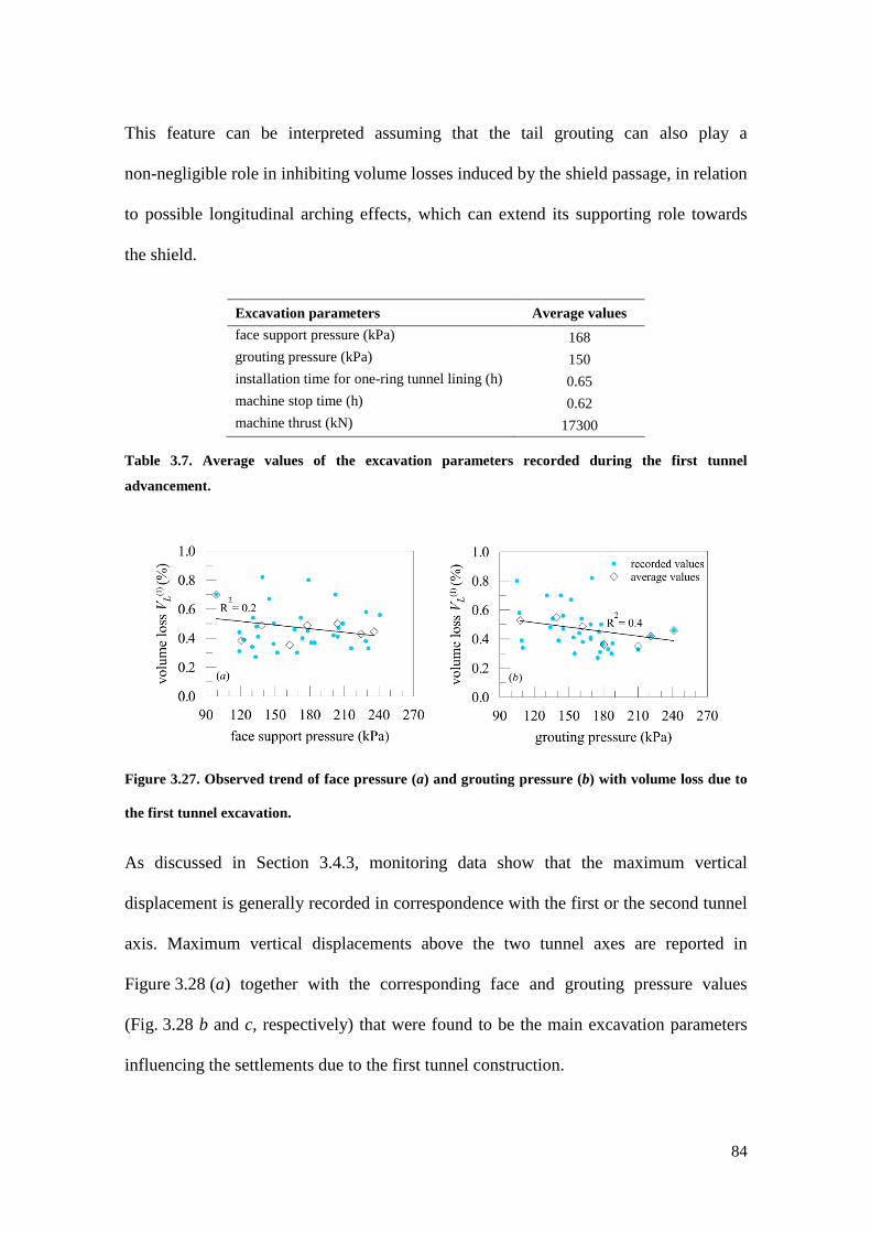
84

This feature can be interpreted assuming that the tail grouting can also play a

non-negligible role in inhibiting volume losses induced by the shield passage, in relation

to possible longitudinal arching effects, which can extend its supporting role towards

the shield.

Excavation parameters Average values

face support pressure (kPa) 168

grouting pressure (kPa) 150

installation time for one-ring tunnel lining (h) 0.65

machine stop time (h) 0.62

machine thrust (kN) 17300

Table 3.7. Average values of the excavation parameters recorded during the first tunnel

advancement.

Figure 3.27. Observed trend of face pressure (a) and grouting pressure (b) with volume loss due to

the first tunnel excavation.

As discussed in Section 3.4.3, monitoring data show that the maximum vertical

displacement is generally recorded in correspondence with the first or the second tunnel

axis. Maximum vertical displacements above the two tunnel axes are reported in

Figure 3.28 (a) together with the corresponding face and grouting pressure values

(Fig. 3.28 b and c, respectively) that were found to be the main excavation parameters

influencing the settlements due to the first tunnel construction.

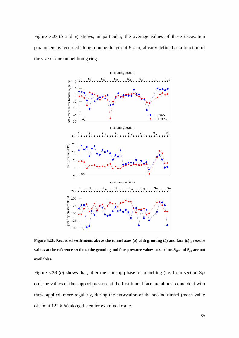
85

Figure 3.28 (b and c) shows, in particular, the average values of these excavation

parameters as recorded along a tunnel length of 8.4 m, already defined as a function of

the size of one tunnel lining ring.

Figure 3.28. Recorded settlements above the tunnel axes (a) with grouting (b) and face (c) pressure

values at the reference sections (the grouting and face pressure values at sections S29 and S30 are not

available).

Figure 3.28 (b) shows that, after the start-up phase of tunnelling (i.e. from section S17

on), the values of the support pressure at the first tunnel face are almost coincident with

those applied, more regularly, during the excavation of the second tunnel (mean value

of about 122 kPa) along the entire examined route.

86

Concerning the grouting pressure, it is possible to observe (Fig. 3.28 c) a larger

variability of the recorded data during the whole excavation of the first tunnel with

respect to the second one, despite the rather similar average values (equal to 150 kPa

and 170 kPa for the first and the second tunnel, respectively).

No statistic correlations between such excavation parameters and the recorded final

settlements emerge from the analysis of the data. It is possible to highlight, however,

some trends in specific areas of the route.

In particular, the sections interested by rather constant settlements above the two tunnel

axes (e.g. from section S18 to section S26) are also characterised by rather regular values

of the face pressure (Fig. 3.28 a, b). In some occasional cases, a decrease in the face

support pressure is associated to an increase in the settlement (e.g. section S28) and vice

versa (e.g. section S31).

Moreover, it is possible to notice that, in general, the higher the settlement above the

first tunnel axis, the lower the values of the grouting pressure (Fig. 3.28 a, c). In

particular, the monitoring sections interested by higher vertical displacements above the

first tunnel axis are also characterised by larger settlements above the second one,

despite the generally larger values of the grouting pressure applied for the second

excavation.

3.4.5 Structural monitoring

The data presented and discussed in this section are vertical displacements recorded

during the excavation of the twin tunnels of the metro-line 5 in correspondence with a

9-storey reinforced concrete framed structure (Fig. 3.29) located nearby the ground

section S35 between Lotto and Portello stations (see Fig. 3.17) and diagonally

undercrossed by the first tunnel (Fig. 3.30).

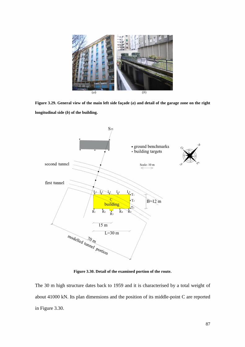
87

Figure 3.29. General view of the main left side façade (a) and detail of the garage zone on the right

longitudinal side (b) of the building.

Figure 3.30. Detail of the examined portion of the route.

The 30 m high structure dates back to 1959 and it is characterised by a total weight of

about 41000 kN. Its plan dimensions and the position of its middle-point C are reported

in Figure 3.30.

88

The building inter-storey height is equal to 3.2 m, with the exception of the ground floor

and of the basement floor, having a height of 4.2 m and 2.5 m, respectively.

The main structural components of the building have the following dimensions: the

sections of the beams are equal to 40 cm x 45 cm at the lower floors, 70 cm x 20 cm and

45 cm x 20 cm within or along the perimeter of the upper floors, respectively; the

column section is equal to 40 cm x 40 cm; the floor slab thickness is of 26 cm at the

lower floors and 22 cm at the upper ones; the sections of the reinforced concrete interior

panels are equal to 0.2 m x 3.26 m.

The structure is founded on five strip footings (0.65 m high, indicated as FI, FII, FIII, FIV

and FV in Fig. 3.31) at 4 m below the ground surface; more specifically, the building

rests on the foundation beams FI, FII and FIII, while the garage zone (Fig. 3.29 b),

situated at the basement floor level along the right longitudinal side of the structure,

stands on the other ones (FIV and FV). Three raft foundations (0.7 m high, indicated as

FVI, FVII and FVIII in Fig. 3.31) are located at the same level under the elevator shafts and

the stairwell, both situated on the right longitudinal side of the building. Reinforced

concrete retaining walls (40 cm thick and 3.5 m high) surround the buried portion of the

structure along its three sides, with the exception of the right longitudinal side for the

access to the garage zone.

Several ground benchmarks (from 5 to 9) were installed on each instrumented ground

section, while building targets were placed along the base of the longitudinal façades

and on its transversal right side (Fig. 3.30). Structural vertical displacements were

gathered during tunnelling by the monitoring targets identified by capital letters L, R

and T and a sequential number in Figure 3.30. The target relative distance and their

distance from the tunnel axes are listed in Tables 3.8 and 3.9, respectively.

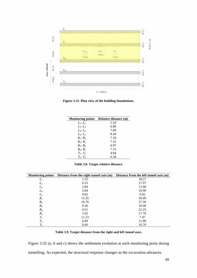
89

Figure 3.31. Plan view of the building foundations.

Monitoring points Relative distance (m)

L1- L2 5.54

L2- L3 6.80

L3- L4 7.09

L4- L5 8.44

R1- R2 7.18

R2- R3 7.32

R3- R4 6.97

R4- R5 7.33

T1- T2 4.84

T2- T3 6.38

Table 3.8. Target relative distance.

Monitoring points Distance from the right tunnel axis (m) Distance from the left tunnel axis (m)

L1 1.53 18.27

L2 0.33 17.07

L3 2.84 13.90

L4 5.84 10.90

L5 9.82 6.92

R1 13.35 30.09

R2 10.76 27.50

R3 9.26 26.00

R4 4.51 21.25

R5 1.02 17.76

T1 11.23 7.47

T2 6.89 11.80

T3 0.00 16.70

Table 3.9. Target distance from the right and left tunnel axes.

Figure 3.32 (a, b and c) shows the settlement evolution at each monitoring point during

tunnelling. As expected, the structural response changes as the excavation advances.

90

Along the longitudinal sides of the building the subsidence profile is characterised by a

hogging-type mode of deformation when the face of the first TBM is located in

correspondence with the middle of the structure (measurements recorded on 11.1.2013),

while the deformative pattern seems to be mainly of sagging-type after the first tunnel

passage (i.e. from 15.01.2013 on). Measurements gathered on 15.1.2013, when the

distance of the first tunnel face from section S35 was about 50 m (i.e. about 8D), range

from 4.7 mm to 6.5 mm along the longitudinal left façade, from 3.5 mm to 6.6 mm

along the longitudinal right one and from 4.6 mm to 5.7 mm along the transversal side.

In particular, it is possible to note that the monitoring targets closer to the first tunnel

axis (i.e. points L1, L2, L3 along the longitudinal left side; R4, R5 along the

longitudinal right side; T2, T3 along the transversal one) are characterised by higher

settlements.

On 18.1.2013 the face of the second EPB machine approached the ground section S35.

As shown in Figure 3.32, settlements increase with the advancement of the second

excavation and the subsidence pattern changes: larger increments in the vertical

displacements are progressively observed, in particular in correspondence with the

targets closer to the second tunnel along the left longitudinal side (i.e. points L4 and L5)

and along the transversal one (point T1). Conversely, the right longitudinal side of the

structure shows a modest increment in the settlement profile with progressively larger

vertical displacements from R1 to R5 and an increasing maximum differential

settlement (Fig. 3.32 b).

When the second tunnel is about 30 m far from the building, i.e. about 5D,

(measurements recorded on 24.1.2013), the settlements reach the final configuration:

they are included in the intervals 8.4 mm - 10.6 mm, 4.1 mm - 8.1 mm and

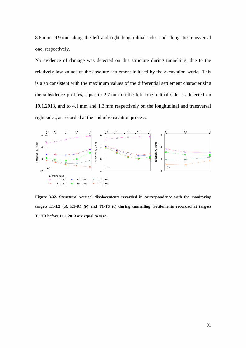
91

8.6 mm - 9.9 mm along the left and right longitudinal sides and along the transversal

one, respectively.

No evidence of damage was detected on this structure during tunnelling, due to the

relatively low values of the absolute settlement induced by the excavation works. This

is also consistent with the maximum values of the differential settlement characterising

the subsidence profiles, equal to 2.7 mm on the left longitudinal side, as detected on

19.1.2013, and to 4.1 mm and 1.3 mm respectively on the longitudinal and transversal

right sides, as recorded at the end of excavation process.

Figure 3.32. Structural vertical displacements recorded in correspondence with the monitoring

targets L1-L5 (a), R1-R5 (b) and T1-T3 (c) during tunnelling. Settlements recorded at targets

T1-T3 before 11.1.2013 are equal to zero.

92

4. Preliminary numerical study on the key ingredients of the

interaction problem: the soil, the tunnel and the structure

4.1 Purpose of Chapter 4

This chapter is focused on the results of a preliminary study, performed by the finite

element code Plaxis (Plaxis, 2012), aimed at investigating the response of the main

ingredients influencing the analysis of a soil-tunnel-structure interaction problem.

The first part of the chapter is devoted to the soil constitutive model adopted in the

numerical study (i.e. Hardening Soil model with small strain stiffness, HSsmall; Benz,

2007). This model is firstly presented and explored; then, it is used in a

two-dimensional (2D) finite element study to describe the mechanical response of a soil

layer interested by the excavation of a single tunnel. A comparison with the steady-state

surface settlements recorded under free-field conditions at a monitoring section of the

Milan metro-line 5 is proposed to validate the performance of the adopted constitutive

formulation in this class of problems.

The excavation of the first and the second tunnel of the metro-line is then simulated

under free-field conditions by a three-dimensional (3D) step-by-step procedure.

Although simplified, the schematisation of the excavation sequence, which principally

aims at simulating the subsidence at the ground surface in a realistic fashion, takes into

account the main aspects of the EPB-tunnelling (e.g. the action of a support pressure

applied at the tunnel face linearly variable with depth, the grouting injection at the

shield tail, the installation of reinforced concrete lining rings, etc.).

In the final part of the chapter the response of a number of structural models subjected

to different loading conditions is analysed by the codes Plaxis 3D and Sap 2000. The

goal of such a comparison is the assessment of the performance of the structural

93

elements in the finite element code adopted in this study as compared to that obtained

by the well-known Sap 2000, a widely used program for structural analyses.

4.2 The constitutive model Hardening Soil with small strain stiffness

4.2.1 Description of the soil constitutive model

The Hardening Soil model with small-strain stiffness (HSsmall; Benz, 2007) is a

constitutive model capable of taking into account the very high soil stiffness observed at

very low strain levels, its reduction with the strain level and the early accumulation of

plastic deformations. It represents an extension of the Hardening Soil model (HS)

developed by Schanz et al. (1999).

The reversible response of the soil is described by an isotropic non-linear elastic law.

The small strain shear modulus, G0, is a function of the stress state by the following

expression:

30 0

' cos ' ' sin '

' cos ' sin '

m

ref

ref

cG G

c p

(4.1)

where G0 ref

is the small strain shear modulus at the reference pressure p ref

= 100 kPa,

′3 is the minimum principal effective stress, m is a constant, c′ is the effective cohesion

and ′ is the angle of shear resistance.

The evolution of the shear modulus with the increase in the shear strain is included in

the constitutive formulation by the expression of the stiffness reduction curve proposed

by Hardin and Drnevich (1972), successively modified by Santos and Correia (2001):

94

0

0 7

1

1

s

.

G

Ga

(4.2)

where Gs is the secant shear modulus, a is a constant equal to 0.385 and γ0.7 is the shear

strain at which the shear modulus is reduced to about 70% of its initial value.

The derivative of Equation (4.2) with respect to the shear strain provides the tangent

shear modulus, Gt, expressed as:

2

0

0 7

1

1

t

.

G

G

a

(4.3)

The tangent shear modulus is bounded by a lower limit corresponding to the shear

modulus Gur:

2 1

ur

t ur

ur

E'G G

( )

(4.4)

This latter is selected by the user, referring to a medium value of the shear strain level,

cut-off, after which the reversible response is characterised by a constant value of the

tangent stiffness with the strain. In Equation (4.4) ur is the Poisson’s ratio for

unloading/reloading.

The expression of cut-off is provided in the following:

00.7

11

0.385

ref

cut off refur

G

G

(4.5)

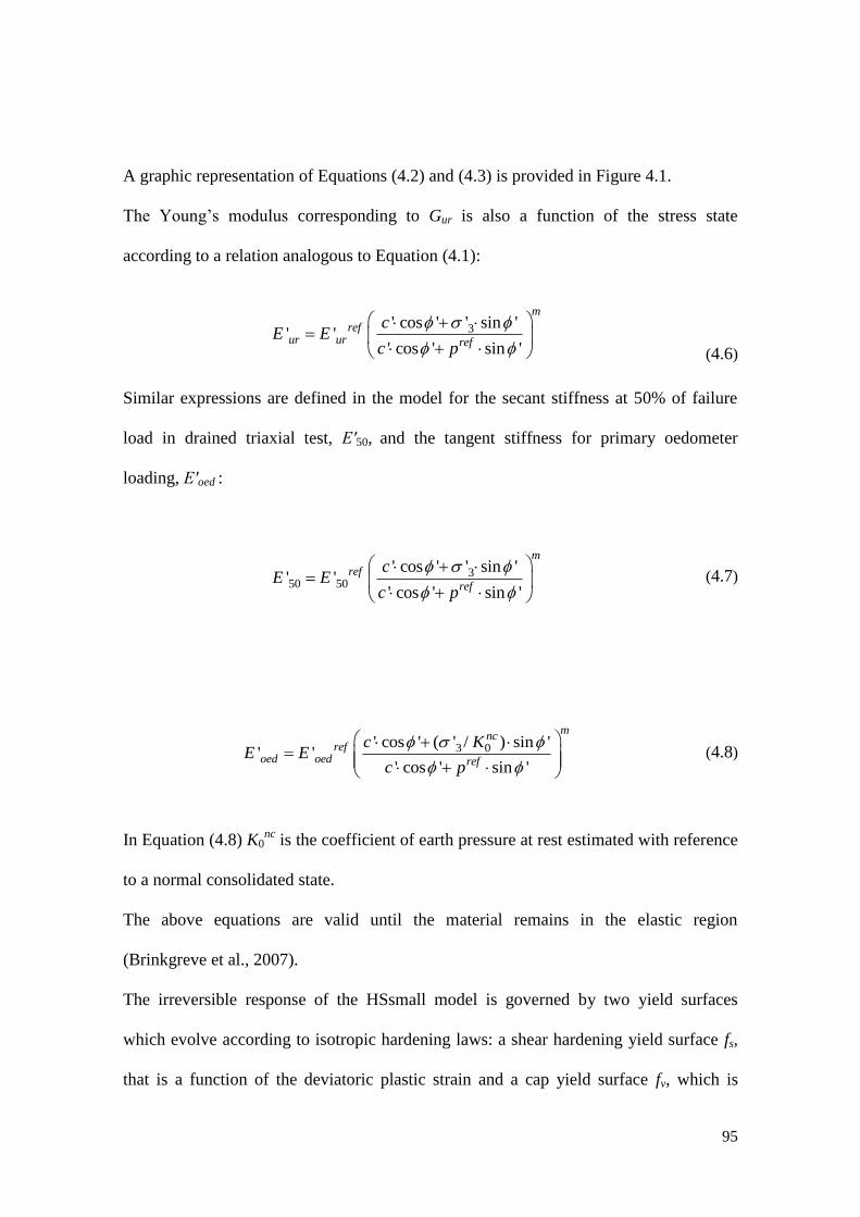
95

A graphic representation of Equations (4.2) and (4.3) is provided in Figure 4.1.

The Young’s modulus corresponding to Gur is also a function of the stress state

according to a relation analogous to Equation (4.1):

3' cos ' ' sin '' '

' cos ' sin '

m

refur ur ref

cE E

c p

(4.6)

Similar expressions are defined in the model for the secant stiffness at 50% of failure

load in drained triaxial test, E′50, and the tangent stiffness for primary oedometer

loading, E′oed :

350 50

' cos ' ' sin '' '

' cos ' sin '

m

ref

ref

cE E

c p

(4.7)

3 0' cos ' ( ' / ) sin '' '

' cos ' sin '

mnc

refoed oed ref

c KE E

c p

(4.8)

In Equation (4.8) K0nc

is the coefficient of earth pressure at rest estimated with reference

to a normal consolidated state.

The above equations are valid until the material remains in the elastic region

(Brinkgreve et al., 2007).

The irreversible response of the HSsmall model is governed by two yield surfaces

which evolve according to isotropic hardening laws: a shear hardening yield surface fs,

that is a function of the deviatoric plastic strain and a cap yield surface fv, which is

96

introduced to bound the elastic region for compressive stress paths and it depends on the

plastic volumetric strain. The elastic region of the model is further reduced for tensile

stress states by means of a tensile cut-off surface. The shear hardening yield surface can

expand up to the ultimate Mohr-Coulomb failure surface.

Figure 4.1. Decay curves of the tangent and secant shear stiffness moduli of the Hardening Soil

model with small strain stiffness.

The flow rule adopted for the cap yield surface fv is associate, while a non-associate rule

is employed for the fs, adopting a formulation inspired by the well-known

stress-dilatancy theory.

4.2.2 Verification and validation of the soil constitutive model

A preliminary study was performed for a first validation of the model, considering an

ideal material having the physical and mechanical properties ( = 18 kN/m3, c′ = 0 kPa,

′ = 30°) of a loose sand (e0 = 0.83). The G0-z profile (Fig. 4.2) was determined

according to the relation proposed by Hardin (1978):

0 '( )

n

m

a a

G pS f e OCR

p p

(4.9)

where f (e) is a function of the void ratio (Hardin and Black, 1968) expressed as:

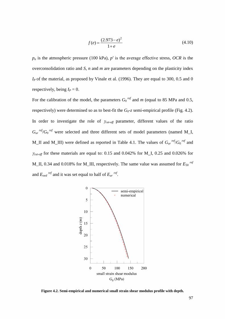
97

2(2.973 )( )

1

ef e

e

(4.10)

pa is the atmospheric pressure (100 kPa), p′ is the average effective stress, OCR is the

overconsolidation ratio and S, n and m are parameters depending on the plasticity index

IP of the material, as proposed by Vinale et al. (1996). They are equal to 300, 0.5 and 0

respectively, being IP = 0.

For the calibration of the model, the parameters G0 ref

and m (equal to 85 MPa and 0.5,

respectively) were determined so as to best-fit the G0-z semi-empirical profile (Fig. 4.2).

In order to investigate the role of cut-off parameter, different values of the ratio

Gur ref

/G0 ref

were selected and three different sets of model parameters (named M_I,

M_II and M_III) were defined as reported in Table 4.1. The values of Gur ref

/G0 ref

and

cut-off for these materials are equal to: 0.15 and 0.042% for M_I, 0.25 and 0.026% for

M_II, 0.34 and 0.018% for M_III, respectively. The same value was assumed for E50 ref

and Eoed ref

and it was set equal to half of Eur ref

.

Figure 4.2. Semi-empirical and numerical small strain shear modulus profile with depth.

98

c′ ′ m G0ref

Eurref

E50ref

Eoedref

0.7 ur

(kPa) (°) (-) (MPa) (MPa) (MPa) (MPa) (%) (-)

M_I 0 30 0.5 85 30 15 15 0.01 0.2

M_II 0 30 0.5 85 50 25 25 0.01 0.2

M_III 0 30 0.5 85 70 35 35 0.01 0.2

Table 4.1. Parameters of the constitutive model assumed for the preliminary study.

Numerical simulations of displacement-control cyclic shearing tests (Fig. 4.3) were

carried out on a weightless soil volume (0.1 m x 0.1 m x 0.1 m) subjected to the

following loading phases:

- isotropic loading (p′=150 kPa; q = 0 kPa);

- isotropic unloading (p′=100 kPa; q = 0 kPa);

- deviatoric loading (p′=133.33 kPa; q = 100 kPa);

- deviatoric unloading (p′=100 kPa; q = 0 kPa);

- cyclic shearing.

In order to obtained the required deformation level (), in the last phase of the test a

horizontal displacement distribution was applied on the soil volume; it is uniform on the

head of the sample, while it linearly decreases with depth along its lateral faces. The soil

volume is fixed at the base. The material is characterised by an initial strain of elastic

type, due to the isotropic and deviatoric loading/unloading process, which produces the

expansion of the yield surface and, consequently, of the elastic domain.

Figure 4.3. Numerical simulation of cyclic shearing tests on a soil sample (0.1 m x 0.1 m x 0.1 m).

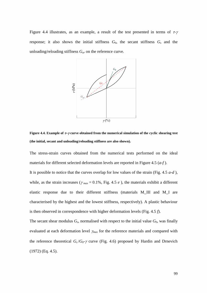
99

Figure 4.4 illustrates, as an example, a result of the test presented in terms of -

response; it also shows the initial stiffness G0, the secant stiffness Gs and the

unloading/reloading stiffness Gur on the reference curve.

Figure 4.4. Example of curve obtained from the numerical simulation of the cyclic shearing test

(the initial, secant and unloading/reloading stiffness are also shown).

The stress-strain curves obtained from the numerical tests performed on the ideal

materials for different selected deformation levels are reported in Figure 4.5 (a-f ).

It is possible to notice that the curves overlap for low values of the strain (Fig. 4.5 a-d ),

while, as the strain increases ( max = 0.1%, Fig. 4.5 e ), the materials exhibit a different

elastic response due to their different stiffness (materials M_III and M_I are

characterised by the highest and the lowest stiffness, respectively). A plastic behaviour

is then observed in correspondence with higher deformation levels (Fig. 4.5 f).

The secant shear modulus Gs, normalised with respect to the initial value G0, was finally

evaluated at each deformation level max for the reference materials and compared with

the reference theoretical Gs /G0- curve (Fig. 4.6) proposed by Hardin and Drnevich

(1972) (Eq. 4.5).

100

Figure 4.5. Stress-strain curves obtained from the numerical cyclic shearing tests at different

deformation levels.

101

The comparison highlights a very good agreement between the computed and

theoretical values for strain levels lower than the reference cut-off, while, as expected, the

two trends diverge for larger values.

Figure 4.6. Comparison between theoretical and numerical Gs /G0- curves for materials M_I, M_II

and M_III.

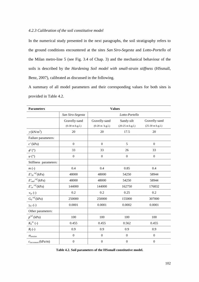
102

4.2.3 Calibration of the soil constitutive model

In the numerical study presented in the next paragraphs, the soil stratigraphy refers to

the ground conditions encountered at the sites San Siro-Segesta and Lotto-Portello of

the Milan metro-line 5 (see Fig. 3.4 of Chap. 3) and the mechanical behaviour of the

soils is described by the Hardening Soil model with small-strain stiffness (HSsmall,

Benz, 2007), calibrated as discussed in the following.

A summary of all model parameters and their corresponding values for both sites is

provided in Table 4.2.

Table 4.2. Soil parameters of the HSsmall constitutive model.

Parameters Values

San Siro-Segesta Lotto-Portello

Gravelly-sand

(0-30 m b.g.l.)

Gravelly-sand

(0-20 m b.g.l.)

Sandy-silt

(20-25 m b.g.l.)

Gravelly-sand

(25-30 m b.g.l.)

(kN/m3) 20 20 17.5 20

Failure parameters:

c′ (kPa) 0 0 5 0

′ (°) 33 33 26 33

ψ (°) 0 0 0 0

Stiffness parameters:

m (-) 0.4 0.4 0.85 0.4

E′50 ref

(kPa) 48000 48000 54250 58944

E′oed ref

(kPa) 48000 48000 54250 58944

E′ur ref

(kPa) 144000 144000 162750 176832

ur (-) 0.2 0.2 0.25 0.2

G0 ref

(kPa) 250000 250000 155000 307000

0.7 (-) 0.0001 0.0001 0.0002 0.0001

Other parameters:

pref

(kPa) 100 100 100 100

K0nc

(-) 0.455 0.455 0.562 0.455

Rf (-) 0.9 0.9 0.9 0.9

tension 0 0 0 0

cincrement (kPa/m) 0 0 0 0

103

The strength parameters (c′ and ′) were determined following what previously

discussed in Section 3.3 of Chapter 3, while the same value for the total unit volume

weight was assumed for the soils above and below the water table. The initial profile of

the horizontal effective stress was calculated using K0nc

values defined in Table 4.2.

The variation of the small strain stiffness with depth was obtained by calibrating the

parameters G0 ref

and m against the down hole experimental results, as shown in Figure

4.7. The assumed shear stiffness decay curves for the gravelly-sand and sandy-silt layers

follow the empirical ones proposed by Vucetic and Dobry (1991) for granular soils

(IP = 0) and for low plasticity silts (IP = 15 %), respectively.

Figure 4.7. Computed and experimental profiles of the small strain shear modulus representative

for the investigated segments of the route.

The reference value of the Young’s modulus at small strains, E′0 ref

, is related to G0 ref

by

the Poisson’s ratio for unloading/reloading, υur. This latter was set equal to 0.20 and

0.25 for the gravelly-sand and for the sandy-silt, respectively. Due to the lack of

laboratory experimental data, the reference unloading/reloading stiffness, E′ur ref

, was

taken equal to 0.24 E′0 ref

for the gravelly-sand

and to 0.42 E′0

ref for the sandy-silt,

104

corresponding to the stiffness values observed along the decay curves at = 0.1%. The

other stiffness parameters, E′50 ref

and E′oed ref

, were assumed three times lower than

E′ur ref

. Finally, standard values were considered for the other parameters of Table 4.2.

For all soil layers the overconsolidation ratio was fictitiously imposed to be large

enough to exclude the activation of the cap yield surface of the constitutive model.

4.2.4 Comparison of measured settlements and computed profiles: the role of the soil

constitutive model

A first numerical analysis was conducted under plane strain conditions using the finite

element code Plaxis 2D (Plaxis, 2012) in order to validate the performance of the

HSsmall constitutive model for this class of problems. With this aim, the final

settlements measured during the construction of the first tunnel of the metro-line along

the initial portion of the route under free-field conditions (i.e. between San Siro and

Segesta stations) were compared with the computed subsidence profile.

The numerical domain was discretised by linear strain 15-node triangular elements.

Nodes at the bottom of the mesh were fixed in both vertical and horizontal directions,

while the vertical boundaries were only fixed in the horizontal direction.

The size of the mesh employed in this study (Fig. 4.8), 80 m wide and 30 m high,

minimises the influence of boundary conditions on the computed results. The domain

was discretised in a total number of 7570 elements having an average dimension of

about 1 m. The hydrostatic water table in the model was fixed at a depth of 15 m below

the ground surface, according to the in situ observations.

The tunnel diameter is equal to D = 6.7 m and the depth of the tunnel axis, z0, was set

equal to 15 m.

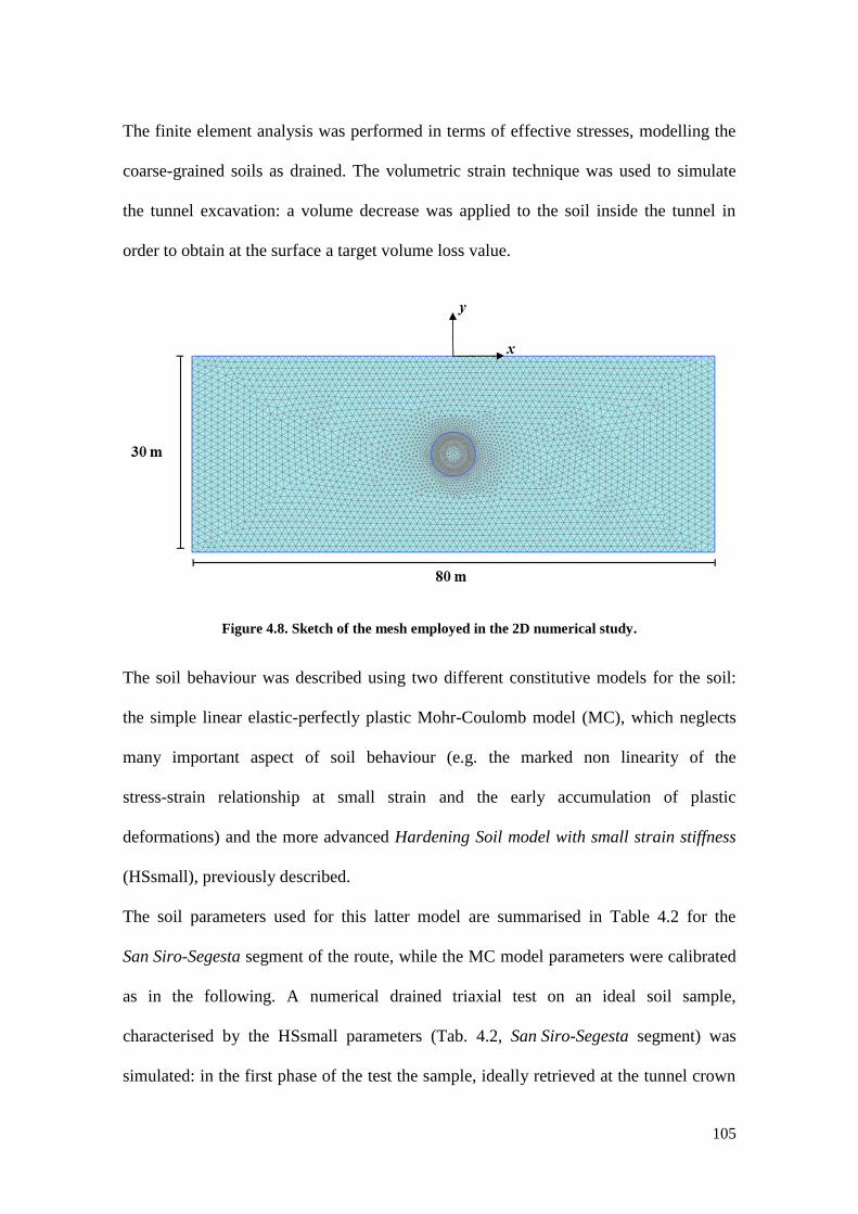
105

The finite element analysis was performed in terms of effective stresses, modelling the

coarse-grained soils as drained. The volumetric strain technique was used to simulate

the tunnel excavation: a volume decrease was applied to the soil inside the tunnel in

order to obtain at the surface a target volume loss value.

Figure 4.8. Sketch of the mesh employed in the 2D numerical study.

The soil behaviour was described using two different constitutive models for the soil:

the simple linear elastic-perfectly plastic Mohr-Coulomb model (MC), which neglects

many important aspect of soil behaviour (e.g. the marked non linearity of the

stress-strain relationship at small strain and the early accumulation of plastic

deformations) and the more advanced Hardening Soil model with small strain stiffness

(HSsmall), previously described.

The soil parameters used for this latter model are summarised in Table 4.2 for the

San Siro-Segesta segment of the route, while the MC model parameters were calibrated

as in the following. A numerical drained triaxial test on an ideal soil sample,

characterised by the HSsmall parameters (Tab. 4.2, San Siro-Segesta segment) was

simulated: in the first phase of the test the sample, ideally retrieved at the tunnel crown

106

depth, was isotropically compressed up to a confining pressure p′ of 150 kPa;

subsequently, a prescribed displacement loading phase was defined in order to simulate

the shearing phase in the test. The resulting stress-strain relationship is shown in Figure

4.9 by a dotted line.

Figure 4.9. Computed stress-strain curves.

The secant Young’s modulus for MC model was selected starting from the HSsmall

stress-strain curve, at the point corresponding to 0.1% strain. Figure 4.9, which also

shows the numerical q-s curve obtained with the MC parameters summarised in Table

4.3, highlights the very high soil stiffness at very low strains and the stiffness reduction

with the strain level as reproduced by the HSsmall model in comparison with the linear

elastic-perfectly plastic response of the MC model.

Parameters Name Value

Failure parameters:

c′ (kPa) effective cohesion 0

′ (°) effective friction angle 33

ψ (°) dilatancy angle 0

Stiffness parameters:

E′ (kPa) Young’s modulus 110000

′ (-) Poisson’s ratio 0.2

Table 4.3. MC model parameters.

107

The reference in situ measurements for the numerical analysis carried out in this study

are the settlements recorded at the monitoring section S16 of the investigated metro-line

segment, that is characterised by a typical value of the volume loss for a

well-performing EPB excavation in coarse-grained soil, i.e. VL = 0.4 %.

Such measurements are reported in Figure 4.10 in comparison with the Gaussian curve

(K = 0.43) and the numerical back-predictions obtained by applying both MC and

HSsmall constitutive models in the analysis.

Figure 4.10. Comparison of monitored settlements, Gaussian curve and computed subsidence

profiles for VL=0.4% at the reference section S16 of the Milan metro-line 5.

As expected, the HSsmall subsidence profile is in agreement with the monitored data

and with their Gaussian interpolation. This indicates, in particular, that the numerical

model is capable of reproducing both maximum settlement and the extension of the

subsidence curve, consistently with what discussed in similar studies proposed in the

literature (e.g. Möller and Vermeer, 2008). Conversely, the MC model clearly

overestimates the extension of the settlement profile, underpredicting its maximum

vertical displacement.

The horizontal displacement Sh (x) profile is presented in Figure 4.11. This figure

illustrates a comparison with the empirical expression proposed by O’Reilly and New

(1982), based on the assumption that the displacement vectors point towards the tunnel

108

axis; no in situ measurements of horizontal displacements were available along the

examined route.

In general, it is possible to observe that the empirical profile is well replicated by the

HSsmall computed trough, with the exception of the maximum value that results

overestimated by the numerical analysis; conversely, the MC profile significantly

diverges from the empirical curve, resulting in sufficient agreement with it only for the

predicted maximum horizontal displacement. However, as reported in the literature (e.g.

Grant, 1998), the displacement vector at the surface is more likely to be directed

towards a point that is shallower than the tunnel axis. Therefore, the empirical

prediction proposed by O’Reilly and New (1982) might underestimate the effective

horizontal component of the displacement.

Figure 4.11. Horizontal displacements: comparison of empirical prediction and computed profiles

for VL=0.4%.

4.3 3D numerical schematisation of TBM-EPB tunnelling

4.3.1 Details of the excavation sequence

The simplified 3D numerical procedure adopted to model the construction of the two

twin tunnels of the Milan metro-line 5 by TBM-EPB machines is illustrated in Figure

4.12.

The first portion of the tunnel cavity is lined by a steel shield, which extends for a total

length of 9.8 m and it is connected to the soil via an interface characterised by the

109

strength parameters of the adjacent soil. In between the shield tail and the permanent

lining, a 1.4 m length of soil is supported by a uniform pressure representing the action

of grouting applied to back-fill the lining after the installation. According to the average

monitored values (see Section 3.4.4 of Chap. 3), the grouting pressure was set equal to

150 kPa and 170 kPa for the first and the second tunnel, respectively.

Figure 4.12. Numerical procedure adopted to simulate TBM-EPB tunnelling.

The shield and the lining were modelled by means of plate structural elements,

characterised by isotropic linear-elastic behaviour, whose properties are listed in Table

4.4.

Parameter Shield Lining

thickness (m) 0.03 0.3

unit volume weight (kN/m3) 75 25

Poisson’s ratio (-) 0.25 0.15

Young’s modulus (GPa) 210 35

Table 4.4. Shield and lining properties.

The excavation of each tunnel was simulated by a step-by-step procedure consisting in

43 advancements, each having the length of one concrete lining ring (1.4 m), from

y = 9.8 m to y =70 m. The advancement consists in removing one slice of soil inside the

tunnel and imposing dry conditions. The tunnel boundaries were considered as

impervious. At each advancement, a pressure was applied at the new tunnel face,

110

corresponding to the theoretical total horizontal stress acting at rest h0 (z), which

ranges from 106 kPa at the tunnel crown to 185 kPa at the invert.

In order to induce a subsidence volume at the ground surface, a fictitious contraction

was applied along the shield, starting from the second slice. Such a contraction, which

determines larger displacements at the top of the section and lower ones at the bottom,

is characterised by a constant increment along each slice, aiming at reproducing in a

simplified way the shield conical geometry. The application of a displacement field at

the tunnel section, however, does not exclude the importance of the adopted constitutive

model, especially for the low values of volume loss that characterise the case under

study, as discussed in the previous Section 4.2.4.

4.3.2 Comparison of computed and measured tunnelling-induced settlements under

free-field conditions

The ability of the numerical simulation of the excavation sequence to reproduce realistic

surface settlement profiles was firstly checked with respect to free-field conditions

(Fargnoli et al., 2015 a).

The numerical study, performed by the finite element code Plaxis 3D (Plaxis, 2012),

refers to the segment of the route between San Siro and Segesta stations, for which

free-field conditions were detected. In this case too, it was taken as an example the

situation of the ground section S16 that is characterised by average values of maximum

settlements and volume loss for the examined portion of the metro-line.

The dimensions of the model shown in Figure 4.13, set up to simulate the twin tunnel

excavation, minimise the influence of the boundary conditions on the computed results.

Nodes at the bottom of the mesh were fixed in both vertical and horizontal directions,

while the vertical boundaries were only fixed in the horizontal directions.

111

The soil domain was discretised by 10-node tetrahedral elements, while 6-node

triangular plate elements were used to model the shield and lining of the tunnels.

According to the in situ stratigraphy, the soil profile is constituted by a single layer of

gravelly-sand and its behaviour was described by the HSsmall constitutive model, using

the parameters reported in Table 4.2 for the San Siro-Segesta segment. The water

surface is located 15 m below the ground surface and it is characterised by a hydrostatic

pore pressure distribution.

The numerical study was performed in terms of effective stresses, assuming for the soil

drained conditions due to the relatively high permeability values measured during the

geotechnical investigation (see Section 3.3 of Chap. 3).

Figure 4.13. Sketch of the mesh for San Siro-Segesta segment of the metro-line 5 under free-field

conditions.

The twin tunnels have a diameter D = 6.7 m and a depth of their axes z0 = 15 m; the

axis-to-axis tunnel horizontal distance, d, is equal to 15 m.

In the numerical analysis, after the initialisation of the stress field in the soil (i.e.

lithostatic conditions), the excavation of each tunnel was simulated in several steps

following the procedure described in the previous section.

112

The contraction applied at the shield of the first tunnel was initially calibrated in order

to reproduce the volume loss due to the first excavation as observed at the ground

section S16 (VL (I)

= 0.40%); then, the same procedure was repeated for the second

tunnel, imposing a different amount of contraction in order to generate the final volume

loss equal to VL (TOT)

= 0.95% (see Tabs. 3.3 and 3.6 of Chap. 3).

The computed surface settlements along the transversal and longitudinal directions,

shown in Figure 4.14 and 4.15 (a, b) respectively, result in agreement with the

measurements recorded at the reference section S16 after the complete excavation of the

first and the second tunnel. The numerical results are also consistent with the

corresponding empirical curves.

Figure 4.14. Comparison of measured, empirical and computed settlements along the transversal

direction after the excavation of the first and the second tunnel under free-field conditions.

For both single and twin tunnel configurations, the computed curves along the

transversal direction nicely replicate the maximum settlements observed above the two

tunnel axes and the extension of the corresponding subsidence trough. The numerical

analysis is also able to capture the interaction phenomena between the tunnels, resulting

113

in an increase in the maximum settlement above the first tunnel axis after the

completion of the second excavation and in a non-symmetric final subsidence profile

that, however, slightly overestimates the measured settlement between the tunnels.

The numerical longitudinal profiles (Fig. 4.15 a and b), though characterised by larger

inflection distances with respect to the empirical ones, are in accordance with

measurements recorded above the two tunnel axes in terms of face settlement (Fig. 4.15

b), settlement due to the shield passage (Fig. 4.15 a) and final values (Fig. 4.15 a and b).

Figure 4.15. Comparison of measured, empirical and computed settlements along the longitudinal

direction after the excavation of the first and the second tunnel under free-field conditions.

The distribution of the vertical strain, z, in the soil at the end of the simulation of the

first and the second tunnel construction is shown in Figure 4.16 (a, b) for the section at

114

y = 35 m (i.e. at a sufficient distance from the model boundaries and from the final

position of the tunnel faces). The figure highlights that, as expected for the considered

K0 value, in both configurations the compressive strains (indicated with negative values

in the figure) are localised at the tunnel lateral zones, while the tensile ones (associated

to positive values) are concentrated at the crown and invert. In particular, after the first

excavation the distribution of the compressive strains around the tunnel is rather

symmetric and characterised by a maximum value of about -0.3%, while the tensile

strains result more concentrated at the invert, with a maximum value equal to about

0.7%. After the second excavation, the soil subjected to compressive strains is not only

localised at the lateral sides of the tunnel, but it extends towards the interaction zone

between the two openings, with maximum values of about -0.5%. The maximum tensile

strains, equal to about 1.5%, are reached in correspondence with the invert of the second

tunnel, due to the larger volume loss imposed in this case.

Figure 4.16. Distribution of the vertical strain z in the soil after the simulation of the first (a) and

the second (b) excavation in correspondence with the tunnel middle-section (y = 35 m) (negative

values indicate compression strains).

4.4 Comparison of the response of structural elements in Plaxis 3D and Sap 2000

The three-dimensional version of the finite element code Plaxis includes a wider choice

of structural elements (such as beams, plates and node-to-node anchors), enhancing its

modelling capability at the cost of a deeper structural competence required to the user.

A number of structural models, where the different structural elements were employed,

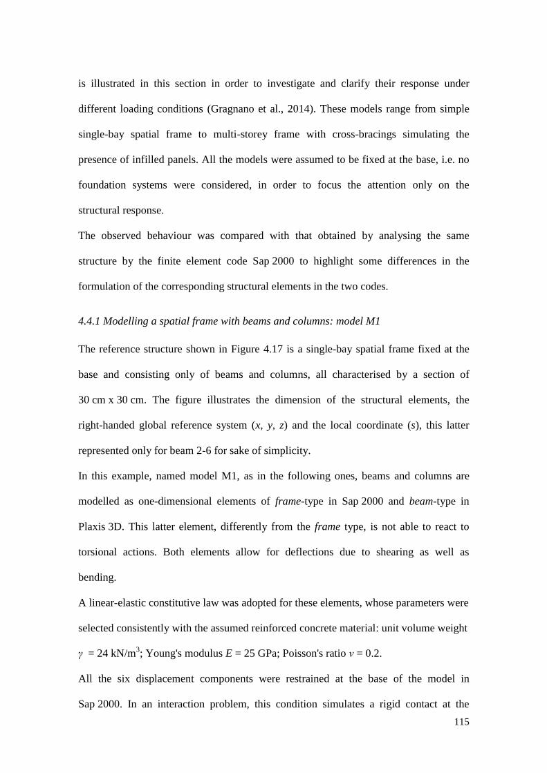
115

is illustrated in this section in order to investigate and clarify their response under

different loading conditions (Gragnano et al., 2014). These models range from simple

single-bay spatial frame to multi-storey frame with cross-bracings simulating the

presence of infilled panels. All the models were assumed to be fixed at the base, i.e. no

foundation systems were considered, in order to focus the attention only on the

structural response.

The observed behaviour was compared with that obtained by analysing the same

structure by the finite element code Sap 2000 to highlight some differences in the

formulation of the corresponding structural elements in the two codes.

4.4.1 Modelling a spatial frame with beams and columns: model M1

The reference structure shown in Figure 4.17 is a single-bay spatial frame fixed at the

base and consisting only of beams and columns, all characterised by a section of

30 cm x 30 cm. The figure illustrates the dimension of the structural elements, the

right-handed global reference system (x, y, z) and the local coordinate (s), this latter

represented only for beam 2-6 for sake of simplicity.

In this example, named model M1, as in the following ones, beams and columns are

modelled as one-dimensional elements of frame-type in Sap 2000 and beam-type in

Plaxis 3D. This latter element, differently from the frame type, is not able to react to

torsional actions. Both elements allow for deflections due to shearing as well as

bending.

A linear-elastic constitutive law was adopted for these elements, whose parameters were

selected consistently with the assumed reinforced concrete material: unit volume weight

γ = 24 kN/m3; Young's modulus E = 25 GPa; Poisson's ratio ν = 0.2.

All the six displacement components were restrained at the base of the model in

Sap 2000. In an interaction problem, this condition simulates a rigid contact at the

116

soil-structure interface, thus being appropriate for the modelling of a soil-foundation

system much stiffer than the superstructure.

Figure 4.17. Spatial frame with beams and columns and global coordinate system.

On the contrary, a foundation plinth 1 m high and characterised by a square section

(1 m x 1 m) was assumed at the base of each column in the Plaxis 3D analysis,

modelled by a two-dimensional plate element. As this code does not allow to perform

numerical analyses without including soil elements, a soil volume (12 m x 15 m x 15 m)

was defined at the base of the frame, assuming for it a very rigid behaviour,

characterised by a Young’s modulus of 750 GPa and a Poisson’s ratio equal to zero.

The response of the model was analysed considering the following loading conditions:

- C1 = gravity loads + uniformly distributed vertical loads equal to 10 kN/m acting on

the beams (Fig. 4.18 a);

- C2 = gravity loads + concentrated vertical loads of 50 kN acting at nodes 3 and 6

(Fig. 4.18 b);

- C3 = gravity loads + concentrated horizontal loads of 50 kN acting at nodes 3 and 6

(Fig. 4.18 c).

117

Numerical analyses were carried out using a finite element mesh of medium density in

Plaxis 3D (i.e. the average size of the finite element is equal to 1.3 m), while adopting

the default option in Sap 2000.

Figure 4.18. Three-dimensional view of model M1 under loading conditions C1 (a), C2 (b) and

C3 (c).

Distributions of shear, bending moment and inflection for beams 6-7 (relative to loading

conditions C1 and C3) and 3-7 (for loading condition C2), as calculated by the two

codes, are shown in Figures 4.19, 4.20 and 4.21.

This latter figure also reports the horizontal displacements along x direction of column

1-2 under loading condition C3.

It is possible to note that the results calculated by Sap 2000 and Plaxis 3D are fairly

coincident in terms of shear, bending moment and inflection, while the horizontal

displacements evaluated for column 1-2 differ in a non-negligible way. Such difference

is due to the characteristics of the beam element in Plaxis 3D which, as anticipated, does

not sustain the torsional action induced by loading condition C3 (Fig. 4.21).

This is confirmed by the results of a further analysis, illustrated in Figure 4.22, identical

to the previous one except for the torsional constraint at the column head which was

removed in the Sap 2000 model: this modification leads to an almost coincident

response as obtained by the two codes.

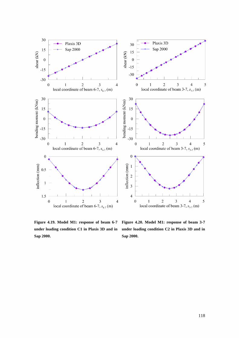
118

Figure 4.19. Model M1: response of beam 6-7

under loading condition C1 in Plaxis 3D and in

Sap 2000.

Figure 4.20. Model M1: response of beam 3-7

under loading condition C2 in Plaxis 3D and in

Sap 2000.

119

Figure 4.21. Model M1: response of beam 6-7 and column 1-2 under loading condition C3 in

Plaxis 3D and in Sap 2000.

Figure 4.22. Model M1: response of beam 6-7 and column 1-2 under loading condition C3 in

Plaxis 3D and in Sap 2000 without torsional constraints at column heads.

120

4.4.2 Modelling a floor slab in a simple spatial frame: model M2

Figure 4.23 shows a single-bay spatial frame differing from the simple structure of

model M1 (see Fig. 4.17) for the presence of a floor slab at the top. A brick-reinforced

concrete floor slab is a structural element having a heterogeneous composition (i.e.

reinforced concrete and brick) and a different stiffness in both plane directions (i.e.

higher stiffness in the warping direction). It is subjected to a plane stress condition and

it is mainly loaded in its out-of-plane direction.

The numerical model of this structure (model M2) is coincident with model M1 in terms

of beams, columns and constraint conditions at the base.

Concerning the floor slab, two different mechanical hypotheses were considered,

namely isotropic and anisotropic. This latter allows to reproduce the main characteristic

of a floor slab, that is a structural element rigid in its own plane and capable of

differentiating the load transferred to the main beams as compared to the secondary

ones.

Figure 4.23. Spatial frame with beams, columns and a floor slab.

The isotropic behaviour was obtained in Plaxis 3D using a two-dimensional

linear-elastic plate element of thickness equal to 25 cm with the following material

121

properties: unit volume weight γ = 32 kN/m3; Young's modulus E = 10 GPa; Poisson's

ratio ν = 0.2.

A two-dimensional shell element with the same geometrical and material properties was

selected to model the isotropic floor slab in Sap 2000.

The presence of a floor slab with anisotropic behaviour was represented in Sap 2000

without simulating the structural element itself, but just applying the constraint

diaphragm to nodes 2, 3, 6 and 7 of Figure 4.23. This constraint, generally used to

model structural components with very high in-plane stiffness, forces the nodes

belonging to the plane of the slab to move together in a rigid way. Assuming the

warping direction of the floor slab along x-axis and according to the current design

practice, the weight of the floor slab was accounted for by applying vertical forces to the

main beams (in y direction) and to the secondary ones (in x direction) with reference to

the influence areas: a load equal to 64.1 kN and 16.8 kN was attributed to the main and

secondary beams, respectively. In particular, the first load is equal to half of the floor

slab weight (80.9 kN, being the total weight equal to 161.8 kN), reduced of the load

(16.8 kN) transferred to the adjacent secondary beams by a floor slab slice 50 cm wide.

When modelling the same slab in Plaxis 3D, an anisotropic elastic model was

employed. More specifically, according to the warping direction along x-axis, the

Young's modulus, Ey, and the shear modulus, Gyz, were reduced as compared to those

adopted in the isotropic case. The amount of the necessary reduction of the moduli to

match the reference results obtained by Sap 2000 is equal to 10%, as such the adopted

parameters are Ey = 1 GPa and Gyz= 416.7 MPa.

The same loading conditions previously analysed for model M1 were considered,

namely C1 (taking also into account the floor slab weight), C2 and C3.

122

The finite element mesh used for this model in Plaxis 3D is similar to that defined in

model M1; in Sap 2000, on the contrary, the mesh of the model with isotropic slab was

modified to make it roughly equivalent to that defined in Plaxis 3D. This expedient is

related to the fact that in Sap 2000 the load of the floor slab is transferred to the beams

in correspondence with the mesh nodes, therefore a similar finite element discretisation

is required in order to obtain consistent results by the two different codes.

Figures 4.24, 4.25 and 4.26 show the comparison between models M1 and M2 in terms

of shear, bending moment and inflection for beam 3-7 under loading conditions C1, C2

and C3, respectively. Figure 4.26 also shows the horizontal displacements of column

1-2 along x-axis.

Results demonstrate the good agreement between the structural responses obtained by

the two different numerical codes. In general, it is possible to observe an equivalent

response of beam 3-7 under loading conditions C1 and C2 for model M2 too.

As expected, the different assumption concerning the behaviour of the floor slab (i.e.

isotropic or anisotropic) plays an essential role in the intensity and distribution of shear,

bending moment and inflection.

In the anisotropic case, the structural element 3-7 is one of two main beams of the floor

slab and it results to be more heavily loaded as compared to what observed in the

isotropic model, where all the beams were equally loaded per unit of length.

On the contrary, the different mechanical hypotheses seem to have a barely relevant

influence on the horizontal displacement of the column: this should be due to the fact

that in both isotropic and anisotropic cases the relevant shear stiffness Gxy assumes the

same value, leading to a similar head restrain acting on the column, therefore resulting

in a correspondingly similar displacement pattern.

123

Figure 4.24. Model M2: response of beam 3-7

under loading condition C1 in Plaxis 3D and in

Sap 2000.

Figure 4.25. Model M2: response of beam 3-7

under loading condition C2 in Plaxis 3D and in

Sap 2000.

124

Figure 4.26. Model M2: response of beam 3-7 and column 1-2 under loading condition C3 in

Plaxis 3D and in Sap 2000.

4.4.3 Modelling a 2D-frame with diagonal elements: model M3

The simple structure shown in Figure 4.27 is a single-bay plane frame with cross

bracings. These elements are commonly adopted in numerical studies to account for

infill panels (e.g.: Panagiotakos and Fardis, 1996). Those latter, although being

non-structural components, significantly contribute to the overall structural response in

the in-plane horizontal direction, leading to a generally stiffer behaviour as compared to

open-frame ones.

In the corresponding numerical model, defined as model M3, the structural elements

(i.e. beam and columns) are represented by frames and beams in Sap 2000 and

Plaxis 3D respectively, and they are characterised by the following material properties:

unit volume weight γ = 24 kN/m3; Young's modulus E = 25 GPa; Poisson's ratio

ν = 0.2.

125

The base of the frame is constrained as in all the other models.

Figure 4.27. 2D frame with cross-bracings.

The diagonal elements of the frame were modelled in order to make them equivalent to

a building infill panel, adopting a simplified version of a formulation proposed in the

literature (Panagiotakos and Fardis, 1996; Fardis, 1997). The width of the cross

bracings, bw, was defined with reference to the expression of Mainstone (1971):

wwhw dhb 4.0)(175.0

(4.11)

where: dw is the diagonal length of the panel, hw is the panel height and the parameter λh

is equal to:

4

4

)2sin(

wcc

wwh

hIE

tE

(4.12)

where Ew and Ec are the Young’s moduli of the infill panel and of the reinforced

concrete structural elements surrounding the panel, respectively; θ is the angle formed

by the diagonal of the infill panel with respect to the horizontal axis; tw is the panel

thickness; Ic is the moment of inertia of the columns adjacent to the infill panel.

The values of these parameters are summarised in Table 4.5.

126

Parameter Value

tw (m) 0.3

hw (m) 4

Ew (GPa) 3

Ec (GPa) 25

Ic (m4) 0.000675

θ (°) 45

λw (1/m) 1.3

dw (m) 5.6

bw (m) 0.5

Table 4.5: Values of the parameters for estimating the equivalent diagonal width, bw.

The cross bracings were modelled as weightless one-dimensional elements reacting

only to axial stress (denoted as truss elements in Sap 2000 and node-to-node anchor

elements in Plaxis 3D), characterised by an axial stiffness equal to K = Ew x bw x tw. An

elasto-plastic constitutive law was selected for such elements to introduce a limit value

of the tensile strength equal to zero. Furthermore, the maximum value of the

compression strength was evaluated according to the following expression:

1 30lim cr wF . τ A

(4.13)

where: τcr is the shear cracking stress of the panel, assumed equal to 0.2 MPa, and Aw is

its transversal area, evaluated as the product of the panel length, lw per its thickness, tw.

The response of model M3 was assessed by considering the structural elements weight

(beams and columns) and a force of 20 kN applied at node 2 along the x-axis (loading

condition C4).

Figure 4.28 shows a perfect match among the results of the two models in terms of

normal stress acting in column 3-4 and diagonal element 2-4; shear, bending moment

and inflection in beam 2-3; horizontal displacement in column 3-4.

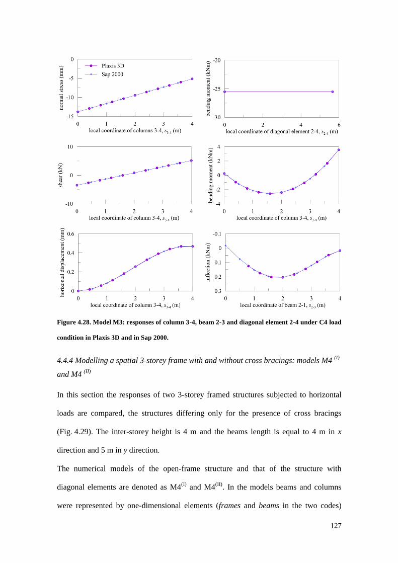
127

Figure 4.28. Model M3: responses of column 3-4, beam 2-3 and diagonal element 2-4 under C4 load

condition in Plaxis 3D and in Sap 2000.

4.4.4 Modelling a spatial 3-storey frame with and without cross bracings: models M4 (I)

and M4 (II)

In this section the responses of two 3-storey framed structures subjected to horizontal

loads are compared, the structures differing only for the presence of cross bracings

(Fig. 4.29). The inter-storey height is 4 m and the beams length is equal to 4 m in x

direction and 5 m in y direction.

The numerical models of the open-frame structure and that of the structure with

diagonal elements are denoted as M4(I)

and M4(II)

. In the models beams and columns

were represented by one-dimensional elements (frames and beams in the two codes)

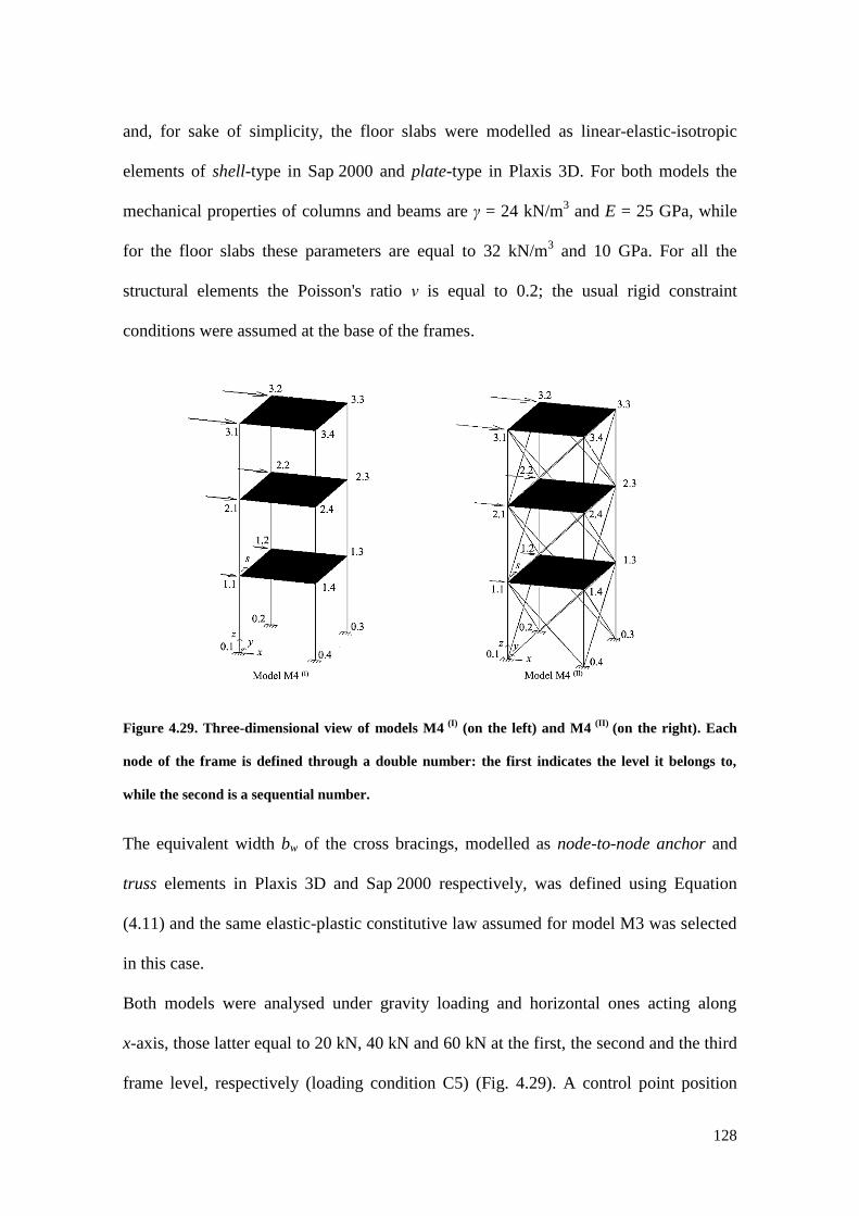
128

and, for sake of simplicity, the floor slabs were modelled as linear-elastic-isotropic

elements of shell-type in Sap 2000 and plate-type in Plaxis 3D. For both models the

mechanical properties of columns and beams are γ = 24 kN/m3 and E = 25 GPa, while

for the floor slabs these parameters are equal to 32 kN/m3 and 10 GPa. For all the

structural elements the Poisson's ratio ν is equal to 0.2; the usual rigid constraint

conditions were assumed at the base of the frames.

Figure 4.29. Three-dimensional view of models M4 (I)

(on the left) and M4 (II)

(on the right). Each

node of the frame is defined through a double number: the first indicates the level it belongs to,

while the second is a sequential number.

The equivalent width bw of the cross bracings, modelled as node-to-node anchor and

truss elements in Plaxis 3D and Sap 2000 respectively, was defined using Equation

(4.11) and the same elastic-plastic constitutive law assumed for model M3 was selected

in this case.

Both models were analysed under gravity loading and horizontal ones acting along

x-axis, those latter equal to 20 kN, 40 kN and 60 kN at the first, the second and the third

frame level, respectively (loading condition C5) (Fig. 4.29). A control point position

129

was selected at the top level (node 3.4) as representative of the horizontal displacement

of the structure.

The horizontal displacement distributions in columns 0.4-1.4, 1.4-2.4, 2.4-3.4 are

reported in Figure 4.30 for both models.

Figure 4.30. Models M4(I)

and M4(II)

: comparison between horizontal displacements obtained in

Plaxis 3D and in Sap 2000 with (on the right) and without (on the left) cross-bracings.

It is worth noting that both codes provide the same results: the maximum horizontal

displacement is equal to 8 cm for model M4(I)

and about 0.8 cm for model M4(II)

. The

outcome of the analyses clearly highlights the effect of claddings on the overall

structural stiffness, although simply accounted for by means of equivalent diagonal

elements: in fact, the presence of cross bracings produces a horizontal displacement

reduction of an order of magnitude as compared to the reference case where they are not

included.

The study presented in this last section should be considered as a preliminary step

towards more complex soil-structure interaction problems, which indeed require a good

level of confidence in the use of structural elements in 3D analyses with Plaxis.

130

The main outcomes resulting from the comparison between the two codes, carried out in

terms of stress and displacements, can be summarised as follows:

- beams and columns can be modelled by frame elements in Sap 2000 and beam

elements in Plaxis 3D. The main difference in the element formulations resides in the

inability of beam elements to react to torsional actions. In fact, the release of torsional

constrains in Sap 2000 produces perfectly matching results;

- the floor slab can be modelled in Sap 2000 by a shell element or using a diaphragm

constraint combined with some additional vertical forces at the top of the columns to

simulate the effect of the slab weight. In the first case an isotropic behaviour is

obtained, while in the latter a more realistic response is reproduced, as it allows to

account for the higher stiffness observed in the warping direction. A plate element is

instead available in Plaxis 3D. The use of an isotropic formulation allows to nicely

reproduce the response of the shell element, while an anisotropic model should be

selected to fit, after a careful calibration of its elastic parameters, the response of the

more advanced scheme of Sap 2000;

- infill panels can be modelled in a simplified manner as cross bracings, whose

characteristics were obtained using the formulation proposed by Mainstone (1971).

Truss and node-to-node anchor elements were used respectively in Sap 2000 and Plaxis

3D, leading to perfectly consistent structural responses.

131

5. 3D numerical modelling of soil-structure interaction during

EPB-tunnelling: an integrated geotechnical and structural approach

5.1 Purpose of Chapter 5

In this chapter the interaction between the ground and multi-storey reinforced concrete

framed structures during tunnelling is investigated by a fully coupled three-dimensional

(3D) approach using the finite element code Plaxis.

The first part of the work is devoted to analyse the response of a number of ideal 2, 4

and 8-storey buildings, with real geometrical and material properties, located in a

symmetric position with respect to a single tunnel. Soil conditions as well as tunnel

characteristics were selected referring to the real case-history of the Milan metro-line 5.

This preliminary interaction analysis is aimed at investigating the modification of the

free-field subsidence troughs, in the transversal and longitudinal directions to the tunnel,

due to the presence of surface structures, specifically evaluating the role of their

stiffness and weight on the absolute and differential settlements.

In the second part of the chapter, the integrated, geotechnical and structural, 3D

numerical study is extended to investigate the response of a real 9-storey reinforced

concrete framed building affected by the settlements induced by the construction of the

Milan metro-line 5. The surface structure is first introduced in the numerical scheme in

detail, taking into account not only its main structural components, but also its

secondary elements (e.g. the external infill-panels). The outcomes of the finite-element

computation, carried out simulating the excavation of both twin tunnels of the line, are

presented and compared with those obtained under free-field conditions and with

monitoring settlement data.

132

Then, the role of the different structural components on the overall behaviour of the

soil-structure system is specifically evaluated, performing additional numerical analyses

with simplified building models, including the equivalent plate schematisation and a

structural model only consisting in the buried portion of the building, properly loaded,

together with its foundation elements. The computed results are finally illustrated and

critically discussed.

5.2 Analysis of ideal multi-storey building response to tunnelling

5.2.1 Finite element model

The different numerical models set up in the present study to simulate an ideal

interaction problem (Boldini et al., 2014) are represented in Figure 5.1 (a-c). In each

scheme the size of the mesh (68 m x 100 m x 30 m) is sufficient to minimise the

influence of boundary conditions on the computed results. As for the scheme of the

free-field numerical analysis previously presented in Section 4.3.2 of Chapter 4, in these

models too the nodes at the bottom of the mesh are fixed in both vertical and horizontal

directions, while the vertical boundaries are only fixed in the horizontal direction.

The soil domain was discretised by 10-node tetrahedral elements. In each model the soil

stratigraphy was defined taking as reference that encountered in situ between the

stations of Lotto and Portello of the line 5 (see Fig. 3.4 of Chap. 3). It is constituted by

two layers of gravelly-sand (between 0-20 m and 25-30 m) and one layer of sandy-silt

(between 20-25 m); the water table was imposed at 15 m below the ground surface. The

soil behaviour was described by the Hardening Soil model with small-strain stiffness

(HSsmall, Benz, 2007), using the calibration reported in Table 4.2 of Chapter 4 for the

reference segment of the route.

The tunnel (D = 6.7 m) is located at a depth of z0 = 15 m and the excavation sequence

follows the steps previously described in Section 4.3.1 of Chapter 4.

133

Figure 5.1. Sketch of the analysed numerical models with ideal multi-storey buildings.

The structural models underpassed by the tunnel are 2, 4 and 8-storey

reinforced concrete framed buildings having a dimension of 24 m x 16 m in plan, an

inter-storey height of 3.2 m and 4 m long bays in both x and y directions. Each structure

134

is founded on 5 strip footings (25.2 m x 1.2 m x 1 m) situated 1 m below the ground

surface and warped along the x-axis; it is composed by beams and columns, both with a

section of 30 cm x 30 cm, and of 22 cm thick floor slabs.

The main structural components were modelled as follows:

- 3-node line beam elements were used for beams and columns;

- 6-node triangular plate elements with isotropic behaviour were used for floor slabs;

- the foundations were modelled by 10 node tetrahedral volume elements constituted by

a non-porous material.

A linear-elastic constitutive law was adopted for these structural components, whose

parameters were selected consistently with the reinforced concrete material properties:

unit volume weight c = 24 kN/m3, Young’s modulus Ec = 25 GPa and Poisson’s ratio

c = 0.2.

The 40 cm thick infill panels, uniformly distributed along the external frames, were

modelled in a simplified way as equivalent cross-bracings (Mainstone, 1971), following

the approach described in Section 4.4.3 of Chapter 4. In this case, however, a reduced

value of Ew = 3 GPa was entered in Equation (4.12) instead of the effective Young’s

modulus of the infill panels (equal to about 6 GPa) in order to take into account the

generally diffuse presence of voids (doors or windows) on the building façades, which

contributes in reducing the overall stiffness of the structures (Melis and Ortiz, 2003).

An interface with a strength controlled by the soil parameters was introduced in the

model solely between the tunnel shield and the soil, while no interfaces were defined at

the soil-lining and soil-building contacts.

135

5.2.2 Numerical analyses and results

All the numerical analyses were performed in terms of effective stresses, assuming

drained conditions for the soils due to the relatively high permeability detected during

the geotechnical investigation.

The finite-element simulations were carried out according to the following steps:

- initialisation of the stress field in the soil (lithostatic conditions);

- activation of the structure in a single step;

- excavation of the first tunnel in several steps (in the first step the displacement field

due to the weight of the building was reset to zero).

In order to calibrate the contraction to be applied at the tunnel profile to reproduce a

target volume loss equal to about 0.3%, a free-field numerical analysis was firstly

performed under free-field conditions (FF analysis) using the procedure previously

validated against measured settlements in Chapter 4 (see Section 4.3). The reference

value of the volume loss corresponds to that observed on average at the Milan

construction site along the Lotto-Portello segment after the excavation of the first tunnel

of the metro-line.

The computed transversal (Fig. 5.2 a) and longitudinal (Fig. 5.2 b) surface profiles are

in fair agreement, respectively, with the Gaussian distribution (Peck, 1969) and the

cumulative Gaussian curve (Mair and Taylor, 1997), this latter translated in order to

take into account the effect of the support pressure acting at the tunnel face. The

comparison between the steady-state computed profiles and the empirical ones, obtained

with K = 0.45 and assuming ix = iy = 6.75 m, although generally satisfactory, highlights

that the transversal and longitudinal inflection distances of the numerical troughs are

slightly larger than the empirical ones (defined by the parameters ix and iy, respectively)

and this comports that the final maximum settlement results rather underestimated.

136

This preliminary FF analysis was followed by the simulations including the structural

models of 2, 4 and 8-storey buildings (STR interaction analyses), all carried out by

imposing the same excavation sequence and amount of contraction defined above.

Figure 5.2. Comparison between numerical and empirical free-field subsidence profiles along

transversal (a) and longitudinal (b) directions for VL=0.31%.

Each structure is characterised by appropriate properties of weight and stiffness, these

latter also enhanced by the inclusion in the structural models of the external

cross-bracings.

The transversal and longitudinal settlement profiles computed by the STR analyses at

the foundation level (i.e. 1 m below the ground surface) are compared in Figure 5.3 (a)

and (b), where the free-field numerical curves (FF) are also shown. In particular, the

proposed transversal troughs are those resulting along section A-A′ of the models (see

Fig. 5.1), i.e. in correspondence with the main building façade.

In general, it is possible to observe that the taller the structure, the larger the maximum

settlement and the extension of the curve as compared to the free-field one, and the

greater the computed VL. This latter feature has to be related to the dependency of the

137

adopted constitutive model on the effective stress state, leading to the non-negligible

role of the weight of the structure.

Figure 5.3 (a) points out that the profiles of the analyses including the structure are

characterised by lower differential settlements with respect to the free-field one, while

they exhibit larger vertical displacements at the building edges, which indicate their

embedment into the soil. Such a result, more evident for the 8-storey structure, is

consistent with observations of centrifuge experiments discussed in the literature (e.g.

Farrell and Mair, 2011).

Figure 5.3 (b) clearly highlights the stiffer response observed in correspondence with

the foundation elements, whose position is reported by dashed lines. It also shows the

non-uniform subsidence profiles under the buildings, to be related to the effect of the

weight distribution.

Figure 5.3. Computed transversal (a) and longitudinal (b) settlement profiles of free-field (FF) and

interaction (STR) analyses with buildings of different height.

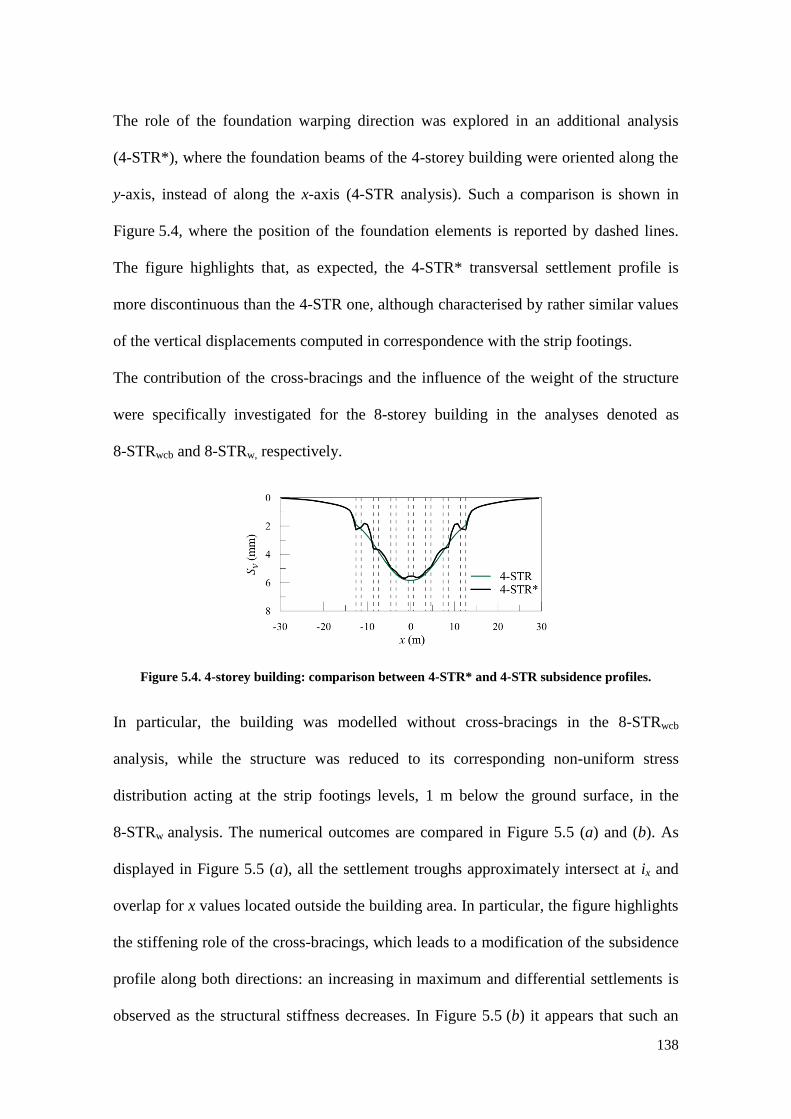
138

The role of the foundation warping direction was explored in an additional analysis

(4-STR*), where the foundation beams of the 4-storey building were oriented along the

y-axis, instead of along the x-axis (4-STR analysis). Such a comparison is shown in

Figure 5.4, where the position of the foundation elements is reported by dashed lines.

The figure highlights that, as expected, the 4-STR* transversal settlement profile is

more discontinuous than the 4-STR one, although characterised by rather similar values

of the vertical displacements computed in correspondence with the strip footings.

The contribution of the cross-bracings and the influence of the weight of the structure

were specifically investigated for the 8-storey building in the analyses denoted as

8-STRwcb and 8-STRw, respectively.

Figure 5.4. 4-storey building: comparison between 4-STR* and 4-STR subsidence profiles.

In particular, the building was modelled without cross-bracings in the 8-STRwcb

analysis, while the structure was reduced to its corresponding non-uniform stress

distribution acting at the strip footings levels, 1 m below the ground surface, in the

8-STRw analysis. The numerical outcomes are compared in Figure 5.5 (a) and (b). As

displayed in Figure 5.5 (a), all the settlement troughs approximately intersect at ix and

overlap for x values located outside the building area. In particular, the figure highlights

the stiffening role of the cross-bracings, which leads to a modification of the subsidence

profile along both directions: an increasing in maximum and differential settlements is

observed as the structural stiffness decreases. In Figure 5.5 (b) it appears that such an

139

effect is more evident in correspondence with the less loaded foundation elements (i.e.

the external strip footings). As expected, the largest maximum and differential

settlements are obtained by neglecting the overall stiffness of the structure, i.e. only

considering its own weight (in STRw analysis), despite the small variation in terms of

volume loss.

The analysis of the results was also extended to compare the evolving response shown

during the tunnelling process by the columns composing the main façade of the

structure. Due to symmetry, the sole response of the columns located on the right side of

the building was examined.

Figure 5.5. Comparison of computed settlement profiles of 8-storey building along transversal (a)

and longitudinal (b) directions: the effect of the structural stiffness and weight.

In particular, the normal compressive forces (N) acting at the columns base (z = 0 m and

x = 0 m, x = 4 m, x = 8 m and x = 12 m) are shown in Figure 5.6 (a) and (b) for different

tunnel face positions (indicated by arrows in the figure). It is possible to observe (Fig.

5.6 a) that as the tunnel face is far from to the examined section (e.g. 16.5 m before the

140

section), the columns at x = 0 m, x = 4 m and x = 8 m are characterised by the same N

value. This latter coincides with that due to the building self-weight and it is larger than

that acting in the outer column (x = 12 m).

During tunnel advancement, the normal force decreases in the inner columns (i.e. those

at x = 0 m and x = 4 m), while in the outer ones, affected by lower settlements, it

exhibits an opposite trend. At the end of the excavation sequence, N reaches its

maximum value in the column at x = 12 m, which experiences the lowest vertical

displacement.

Figure 5.6. 8-STR (a) and 8-STRwcb (b) analyses: N values acting in the columns of the 8-storey

building at the excavation progress.

This behaviour is due to the process of force redistribution within the structure, which is

enhanced by the presence of the cross-bracings. The absence of these latter elements in

the numerical model (8-STRwcb analysis) inhibits the load transfer within the structure:

in fact in this case, illustrated in Figure 5.6 (b), N values in the inner columns are rather

constant during tunnelling, while the normal stress evolution in the outer one is similar

to that of Figure 5.6 (a), but for lower values of normal compressive forces.

141

5.3 Numerical simulation of the interaction process between a 9-storey reinforced

concrete framed building and the Milan metro-line 5

5.3.1 Finite element scheme with a detailed structural model

The numerical model (80 m x 100 m x 30 m) set up to simulate the interaction between

the twin tunnels of the metro-line 5 and the investigated multi-storey reinforced

concrete framed building undercrossed by the first tunnel (Fargnoli et al., 2015 a) is

shown in Figure 5.7. It neglects, for sake of simplicity, the presence of other nearby

constructions and its dimension minimises the influence of boundary conditions on the

computed results.

The soil profile refers to the subsoil conditions encountered between Lotto and Portello

stations (the segment of the route where the building is located) and it was defined

according to the in situ stratigraphy. As for the previous numerical analyses, in this case

too the mechanical behaviour of the soils was described by the Hardening soil model

with small strain stiffness using the parameters summarised in Table 4.2 of the previous

chapter.

The tunnels have a diameter D = 6.7 m and their axes, having a horizontal distance d

equal to 16.7 m, are located at a depth of z0 = 15 m, as in the reference case of study in

correspondence with the ground section S35 nearby the building (see Fig. 3.30 of Chap.

3), also represented in Figure 5.7.

The simulation of each tunnel excavation was performed by the step-by-step numerical

procedure already described in detail and validated in Section 4.3.2 (see Chap. 4), using

the same values of the face and grouting pressures.

In the model of Figure 5.7, the first tunnel underpasses the building according to the real

tunnel-structure relative position. In particular, the rotation angle of the longitudinal

sides of the building with respect to the tunnel axes is set equal to 25.14° and the x and y

142

coordinates of the structure’s middle point C (see Fig. 3.30 of Chap. 3) are equal to 0 m

and 35 m, respectively.

Figure 5.7. Detail of the mesh used in the numerical model with the building and the twin tunnels.

In the structural model of the building:

- beams and columns were modelled by beam elements;

- floor-slabs, reinforced concrete interior panels, elevator shafts, stairwell and retaining

walls were modelled using plate elements;

- foundations were modelled using volume elements constituted by non-porous material.

A linear-elastic constitutive law was selected for all the structural components,

considering material properties appropriate for the reinforced concrete (i.e.

c = 24 kN/m3; Ec = 25 GPa; c = 0.2).

The building is characterised by the presence of infill panels, uniformly distributed

along the external frames, which were modelled, in this case too, in a simplified way by

means of equivalent cross-bracings following Mainstone (1971) (see Section 5.2). In

this model, however, in order to introduce a more realistic value of the maximum tensile

strength, F T lim, it was assumed to be equal to 0.1 F C

lim.

143

The pressure distribution of this structure at the foundation level is shown in Figure 5.8.

It is possible to observe, in particular, higher pressure values in correspondence with the

elevator shafts (FVI and FVIII) and the stairwell (FVII), i.e. the heavier components of the

building.

Figure 5.8. Pressure distribution at the foundation level of the building.

5.3.2 Results of the numerical analysis with a detailed structural model

The first part of the finite element study was devoted to simulate the excavation of the

first tunnel which directly interacts with the reference building.

Such simulation was firstly performed without activating the surface structure in the

model (under free-field conditions, i.e. numerical analysis defines as FF) in order to

calibrate the contraction to be applied at the tunnel shield to reproduce a volume loss

VL (I)

equal to 0.34%, which corresponds to that observed at the monitoring ground

section nearby the building (i.e. section S35, see Tab. 3.5 of Chap. 3). In particular, such

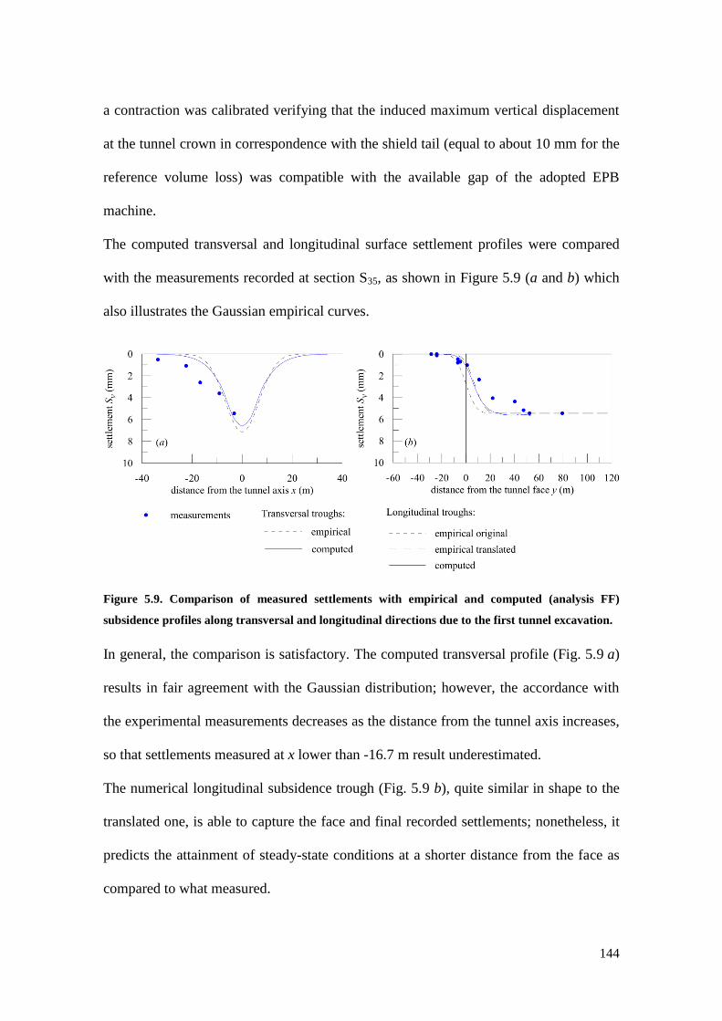
144

a contraction was calibrated verifying that the induced maximum vertical displacement

at the tunnel crown in correspondence with the shield tail (equal to about 10 mm for the

reference volume loss) was compatible with the available gap of the adopted EPB

machine.

The computed transversal and longitudinal surface settlement profiles were compared

with the measurements recorded at section S35, as shown in Figure 5.9 (a and b) which

also illustrates the Gaussian empirical curves.

Figure 5.9. Comparison of measured settlements with empirical and computed (analysis FF)

subsidence profiles along transversal and longitudinal directions due to the first tunnel excavation.

In general, the comparison is satisfactory. The computed transversal profile (Fig. 5.9 a)

results in fair agreement with the Gaussian distribution; however, the accordance with

the experimental measurements decreases as the distance from the tunnel axis increases,

so that settlements measured at x lower than -16.7 m result underestimated.

The numerical longitudinal subsidence trough (Fig. 5.9 b), quite similar in shape to the

translated one, is able to capture the face and final recorded settlements; nonetheless, it

predicts the attainment of steady-state conditions at a shorter distance from the face as

compared to what measured.

145

The overall consistency of the computed profiles with the empirical solutions and with

available measurements indicates that the adopted numerical model is amenable to be

adopted for more complex interaction analyses, as illustrated in the following.

With the aim to investigate the interaction between the first tunnel and the building, this

latter was included in the numerical model and the computation was repeated imposing

the same excavation sequence adopted in FF analysis, thus assuming that no relevant

changes in volume losses occurred between the ground section S35 and the structure.

This interaction analysis, defined as STR, was performed accounting for the appropriate

weight and stiffness of the structural elements, including in the model the external

cross-bracings.

The numerical final settlement troughs, as computed along the transversal and

longitudinal directions to the tunnel axis at the foundation level (i.e. 4 m below the

ground surface), are compared to the corresponding free-field predictions in Figure

5.10 (a) and (b). The plant position of the foundation elements is also shown by dashed

lines. In particular, the figure refers to the subsidence profiles computed at the

barycentre of the building (point C in Fig. 3.30 of Chap. 3).

As expected, the presence of the building influences the settlement profiles which

deviate from the free-field ones along both directions, highlighting the stiffer response

observed in correspondence with the discrete foundation elements. The two profiles

only overlap outside the building area. It is worth noting that the maximum vertical

displacement and volume loss of the interaction analysis are larger than the free-field

one, due to the effect of the building weight. Such an observation is particularly evident

at the stairwell (FVII in Fig. 5.10 a) and at the elevator shaft (FVI in the same figure), i.e.

in correspondence with the heavier components of the building.

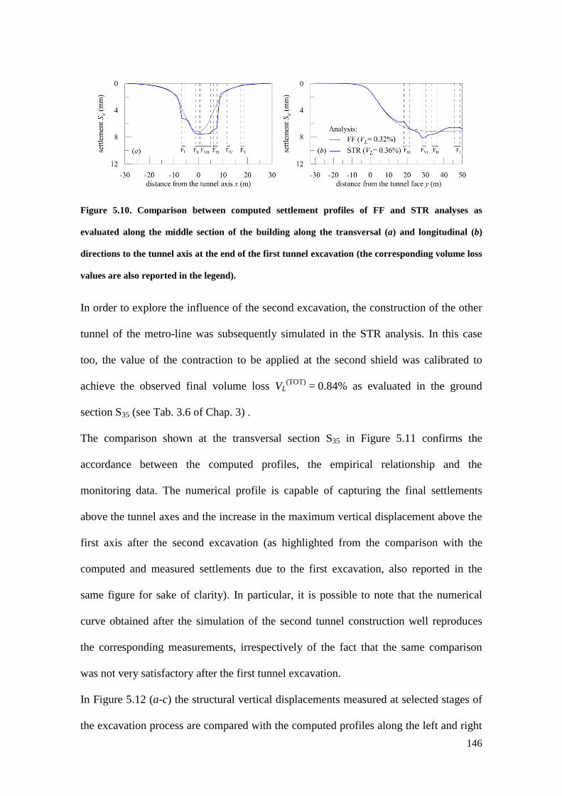
146

Figure 5.10. Comparison between computed settlement profiles of FF and STR analyses as

evaluated along the middle section of the building along the transversal (a) and longitudinal (b)

directions to the tunnel axis at the end of the first tunnel excavation (the corresponding volume loss

values are also reported in the legend).

In order to explore the influence of the second excavation, the construction of the other

tunnel of the metro-line was subsequently simulated in the STR analysis. In this case

too, the value of the contraction to be applied at the second shield was calibrated to

achieve the observed final volume loss VL(TOT)

= 0.84% as evaluated in the ground

section S35 (see Tab. 3.6 of Chap. 3) .

The comparison shown at the transversal section S35 in Figure 5.11 confirms the

accordance between the computed profiles, the empirical relationship and the

monitoring data. The numerical profile is capable of capturing the final settlements

above the tunnel axes and the increase in the maximum vertical displacement above the

first axis after the second excavation (as highlighted from the comparison with the

computed and measured settlements due to the first excavation, also reported in the

same figure for sake of clarity). In particular, it is possible to note that the numerical

curve obtained after the simulation of the second tunnel construction well reproduces

the corresponding measurements, irrespectively of the fact that the same comparison

was not very satisfactory after the first tunnel excavation.

In Figure 5.12 (a-c) the structural vertical displacements measured at selected stages of

the excavation process are compared with the computed profiles along the left and right

147

longitudinal façades of the building and along its transversal side. In particular,

reference is made to the observations carried out for a position of the first tunnel face at

the middle of the structure (point C in Fig. 3.30 of Chap. 3) and at the end of the first

and the second excavation, respectively.

Figure 5.11. Comparison of measured settlements induced by the first and the second tunnel at

ground transversal section S35 with numerical curves (the Gaussian empirical curves are also shown

in the plot).

The numerical analysis, properly taking into account the geometry, the stiffness and the

weight of the building, provides subsidence profiles along each building façade that

well reproduce the measured vertical displacements in terms of both shape and single

values. In general, the finite element computation accurately predicts the deformative

pattern of the building, realistically capturing the evolution from hogging to sagging

configurations during the different phases of tunnelling. In fact, the hogging and

sagging zones are highlighted along the left and right longitudinal building façades (Fig.

5.12 a and b), where the settlement troughs are more continuous than that observed

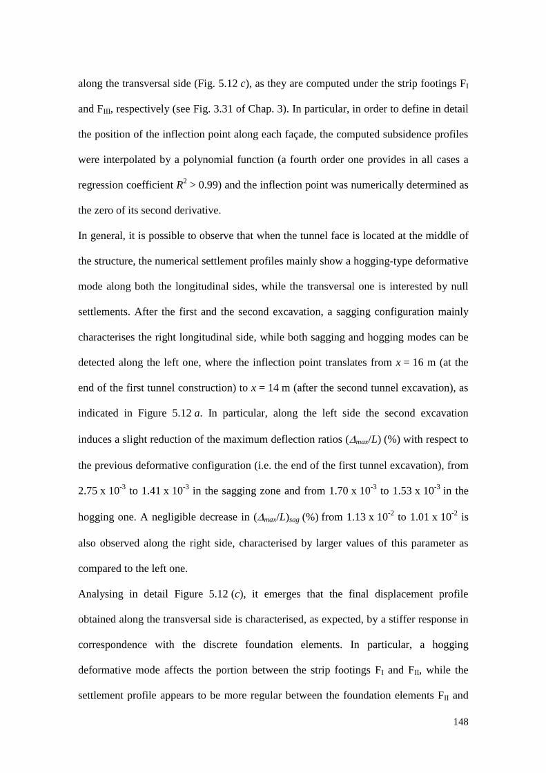
148

along the transversal side (Fig. 5.12 c), as they are computed under the strip footings FI

and FIII, respectively (see Fig. 3.31 of Chap. 3). In particular, in order to define in detail

the position of the inflection point along each façade, the computed subsidence profiles

were interpolated by a polynomial function (a fourth order one provides in all cases a

regression coefficient R2 > 0.99) and the inflection point was numerically determined as

the zero of its second derivative.

In general, it is possible to observe that when the tunnel face is located at the middle of

the structure, the numerical settlement profiles mainly show a hogging-type deformative

mode along both the longitudinal sides, while the transversal one is interested by null

settlements. After the first and the second excavation, a sagging configuration mainly

characterises the right longitudinal side, while both sagging and hogging modes can be

detected along the left one, where the inflection point translates from x = 16 m (at the

end of the first tunnel construction) to x = 14 m (after the second tunnel excavation), as

indicated in Figure 5.12 a. In particular, along the left side the second excavation

induces a slight reduction of the maximum deflection ratios (max/L) (%) with respect to

the previous deformative configuration (i.e. the end of the first tunnel excavation), from

2.75 x 10-3

to 1.41 x 10-3

in the sagging zone and from 1.70 x 10-3

to 1.53 x 10-3

in the

hogging one. A negligible decrease in (max/L)sag (%) from 1.13 x 10-2

to 1.01 x 10-2

is

also observed along the right side, characterised by larger values of this parameter as

compared to the left one.

Analysing in detail Figure 5.12 (c), it emerges that the final displacement profile

obtained along the transversal side is characterised, as expected, by a stiffer response in

correspondence with the discrete foundation elements. In particular, a hogging

deformative mode affects the portion between the strip footings FI and FII, while the

settlement profile appears to be more regular between the foundation elements FII and

149

FIII, where the final deformative pattern corresponds to an almost rigid rotation if

evaluated with respect to the previous configuration (i.e. that at the end of the first

excavation).

Figure 5.12. Comparison of settlements measured along the left (a) and right (b) longitudinal sides

of the building and along its transversal one (c) at different phases of twin tunnel excavation (on the

transversal side the position of the foundation beams is also indicated by dashed lines).

Field observations demonstrate that typically structures are more vulnerable to hogging

deformative modes as compared to sagging ones (e.g. Burland et al., 2001), as

settlements may induce cracks in the upper portions where the constructions are not

constrained by ground and foundation elements and, as such, they are more prone to

150

deform. However, differently from masonry structures, the presence of closed frames in

reinforced concrete buildings confines the crack propagation, generally preventing

severe damages to occur (Son and Cording, 2011).

Figure 5.13 presents an attempt to investigate this aspect of the structural response, by

plotting the normal stresses acting within the cross-bracings of the longitudinal façades

while the building experiences a predominantly hogging-type mode of deformation, i.e.

when the first tunnel face is located at the middle of the structure. The figure also

includes the corresponding computed subsidence profiles and the relative values of the

deflection ratio (max/L)hog (Burland and Wroth, 1974; Burland et al., 2004).

Larger normal compressive stresses (c) are observed at the lower floors, due to the

effect of the structure’s weight. According to the deformative mechanism, the

cross-bracings subjected to normal tensile stresses (t), represented by dashed lines in

the figure, are located in the upper levels of the structure. They tend to concentrate

along the left longitudinal side, which is characterised by larger total and differential

settlements and, consequently, by the highest value of the maximum deflection ratio.

The computed maximum value of the tensile strain, detected on this side and equal to

about 0.004 %, is much lower than the limit value proposed by Boscardin and Cording

(1989) to identify the upper bound of the “negligible” damage category (i.e. 0.05 %);

this is consistent with the absence of damage observed in situ on this structure.

The structural response was also analysed in terms of normal compressive forces (N)

acting at the base (z = 0) of the columns located along the longitudinal façades of the

building at the end of the first tunnel excavation. These values are reported in

Figure 5.14 (a) and (b) together with the settlements computed at the columns’ base at

such selected tunnelling stage.

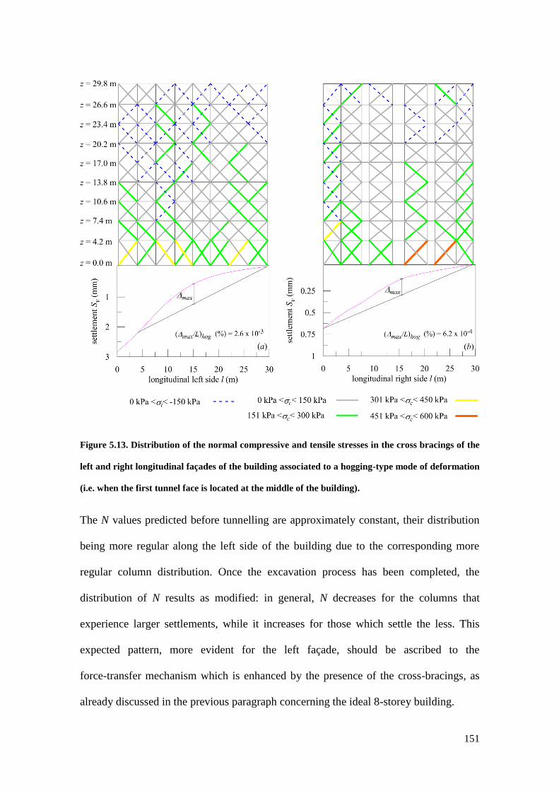
151

Figure 5.13. Distribution of the normal compressive and tensile stresses in the cross bracings of the

left and right longitudinal façades of the building associated to a hogging-type mode of deformation

(i.e. when the first tunnel face is located at the middle of the building).

The N values predicted before tunnelling are approximately constant, their distribution

being more regular along the left side of the building due to the corresponding more

regular column distribution. Once the excavation process has been completed, the

distribution of N results as modified: in general, N decreases for the columns that

experience larger settlements, while it increases for those which settle the less. This

expected pattern, more evident for the left façade, should be ascribed to the

force-transfer mechanism which is enhanced by the presence of the cross-bracings, as

already discussed in the previous paragraph concerning the ideal 8-storey building.

152

Figure 5.14. STR analysis: normal compressive force and settlement values at the base of the

columns on the left (a) and right (b) longitudinal sides of the building before tunnelling and at the

end of the first tunnel construction.

5.3.3 Finite element schemes with simplified structural models

Additional numerical schemes were also set up adopting different levels of detail in the

structural modelling (Fargnoli et al., 2015 b). The analysis was limited to the interaction

with the first tunnel of the metro-line and, in order to reduce the computational effort,

the width of the mesh was reduced from 80 m (see Fig. 5.7) to 68 m, as shown in Figure

5.15.

The simplified structural schemes considered in the numerical study are described in the

following:

- the building was first modelled without cross-bracings (Fig. 5.15 a) in order to

investigate the stiffening role of these components (analysis STRwcb);

- the building was limited to its buried portion (Fig. 5.15 b) in order to evaluate its

stiffening contribution (analysis STRw). This model also includes the foundation

elements and the retaining walls, those latter 0.4 m thick and 3.5 m high, connecting the

foundation level to the ground floor. The upper portion was reduced to an equivalent

load distribution; these loads were evaluated with reference to their influence area and

153

they were applied at the ground floor in correspondence with the columns’ head, the

stairwell and the elevator shafts;

- the structure was strongly simplified and schematised as an equivalent plate (L = 30 m

and B = 12 m) in terms of stiffness and weight (Fig. 5.15 c), placed at the foundation

level (analysis STR*). In this model the retaining walls were also introduced. The input

parameters of the equivalent plate were derived adapting the approach proposed by

Franzius et al. (2006), as discussed in the following.

The axial (EcA)building and bending (EcJ)building stiffness of the building were calculated

considering the structure to consist only of floor slabs and to be oriented with the

longitudinal sides parallel to the tunnel axis (such hypothesis does not significantly

influence the second moment of area of the slab):

1

( ) ( )n

c building c slabE A E A

(5.1)

2

1 1

( ) ( ) ( )n n

c building c slab c slab slab mE J E J E J A H

(5.2)

were:

- n is the reference level of the building;

- Aslab and Jslab are the cross-sectional area and the second moment of area of the slab at

each level, respectively;

- Hm is the vertical distance between the slab’s and the structure’s neutral axis (this

latter assumed to be located in correspondence with the structure’s centroid).

The building foundation system was neglected in this simplified approach (Franzius et

al., 2006).

154

Figure 5.15. Sketch of the finite element models with simplified structural schemes: building

without cross-bracings (a); building reduced to its buried portion (b); building reduced to an

equivalent plate (c).

The computed axial and bending stiffness for each slab are reported in Table 5.1

together with the thickness and Hm values.

155

level, n slab thickness (m) Hm (m) Ec Aslab (kN) Ec Jslab (kNm2)

basement floor 0.26 15.70 1.95E+0.8 1.10E+06

ground floor 0.26 13.20 1.95E+08 1.10E+06

1st floor 0.22 9.00 1.65E+08 6.66E+05

2nd

floor 0.22 5.80 1.65E+08 6.66E+05

3rd

floor 0.22 2.60 1.65E+08 6.66E+05

4th

floor 0.22 0.60 1.65E+08 6.66E+05

5th

floor 0.22 3.80 1.65E+08 6.66E+05

6th

floor 0.22 7.00 1.65E+08 6.66E+05

7th

floor 0.22 10.20 1.65E+08 6.66E+05

8th

floor 0.22 13.40 1.65E+08 6.66E+05

9th

floor 0.22 16.60 1.65E+08 6.66E+05

Table 5.1. Stiffness properties of the slabs at each level.

The input parameters of the plate element used in the FE analyses were then evaluated

as:

12( )

( )

c buildingfe

c building

E Jt

E A

(5.3)

( )c buildingfe

fe

E AE

t

(5.4)

being tfe (equal to 36 m) and Efe (equal to 51.8 GPa) the equivalent thickness and

Young’s modulus, respectively.

The unit volume weight of the plate element, equal to 2.92 kN/m3, was calculated as the

ratio between the total building weight (excluding the weight of the retaining walls

modelled in the analysis, equal to about 2500 kN) and the plate volume (B x L x tfe).

5.3.4 Results of the numerical analyses with simplified structural models

The additional analyses carried out adopting simplified schematisations of the building

aim at highlighting the role of different structural components on the overall stiffness of

the system and, thus, on the computed displacement field.

Figure 5.16 summarises all the monitored and computed settlement profiles as observed

and back-predicted along the longitudinal and transversal sides of the building.

156

The comparison between the STRwcb and STR results proves that the absence of the

cross-bracings does not significantly affect the overall displacement pattern (Fig. 5.16),

while it can play a non-negligible role on the structural forces.

Figure 5.16. Comparison of monitored, empirical and computed settlements at the end of the first

tunnel excavation on the longitudinal left (a) and right (b) sides and on the transversal right side of

the building (d). Empirical and computed settlement profiles on the transversal left side of the

structure, where measurements were not available, are also compared (c).

As shown in Figure 5.17 (a and b), in fact, the absence of these elements reduces the

force redistribution process within the structure: at the end of excavation, the N

distribution is characterised by a different pattern as compared to analysis STR (see Fig.

5.14 a and b), with relatively higher values in the inner columns for the left side of the

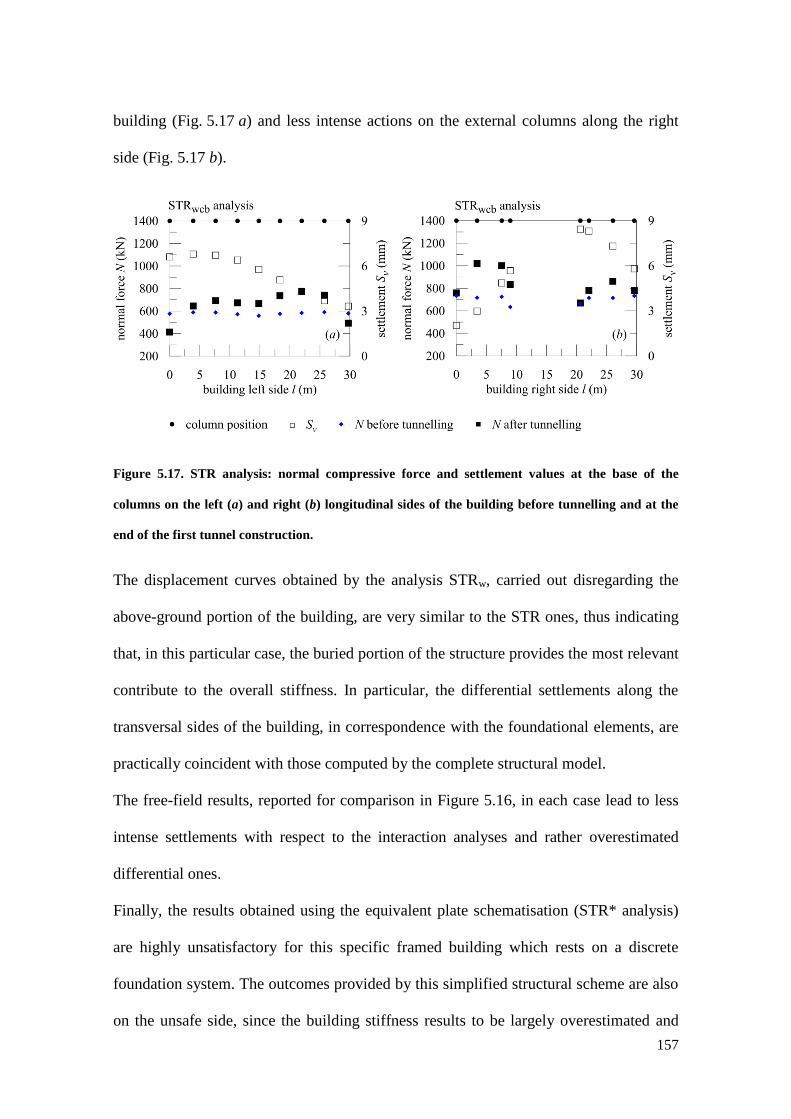
157

building (Fig. 5.17 a) and less intense actions on the external columns along the right

side (Fig. 5.17 b).

Figure 5.17. STR analysis: normal compressive force and settlement values at the base of the

columns on the left (a) and right (b) longitudinal sides of the building before tunnelling and at the

end of the first tunnel construction.

The displacement curves obtained by the analysis STRw, carried out disregarding the

above-ground portion of the building, are very similar to the STR ones, thus indicating

that, in this particular case, the buried portion of the structure provides the most relevant

contribute to the overall stiffness. In particular, the differential settlements along the

transversal sides of the building, in correspondence with the foundational elements, are

practically coincident with those computed by the complete structural model.

The free-field results, reported for comparison in Figure 5.16, in each case lead to less

intense settlements with respect to the interaction analyses and rather overestimated

differential ones.

Finally, the results obtained using the equivalent plate schematisation (STR* analysis)

are highly unsatisfactory for this specific framed building which rests on a discrete

foundation system. The outcomes provided by this simplified structural scheme are also

on the unsafe side, since the building stiffness results to be largely overestimated and

158

the displacement field at the foundation level appears to be characterised by almost rigid

rotations along the four sides of the structure, without indicating any sagging or hogging

deformative modes.

159

6. Conclusions

This research is mainly devoted to analyse the interaction mechanism between a

reinforced concrete framed building and the twin tunnels of an urban metro-line.

Reference is made to in situ settlement monitoring data and results of three-dimensional

(3D) finite element computations performed by a fully-coupled approach, i.e.

incorporating in a unique numerical model the soil, the tunnel and the structure. This

integrated solution, sometimes adopted in the past by other researchers to evaluate the

effects on masonry buildings due to tunnel excavation, has not yet been extended to date

to framed structures schematised with accuracy. As such, one element of novelty of this

study is the detail adopted in modelling an existing multi-storey reinforced concrete

building influenced by tunnelling activities. This topic is nowadays of great relevance

for metro-line construction in urban areas, where structures frequently interact with

underground excavations and, as such, might be damaged.

As discussed in Chapter 2, the empirical approach proposed in the past to predict the

surface subsidence in absence of existing structures on the ground (i.e. under free-field

conditions), considers Gaussian distributions for the settlement profiles induced by

tunnelling in the transversal and longitudinal directions to the tunnel axis. Interaction

phenomena affect the settlements experienced by existing buildings, which differ from

those predicted under free-field conditions by the empirical solutions. These latter, in

fact, neglect the modification of the subsidence profile due to the stiffness and weight of

the structures, often leading to an unrealistic scenario, characterised by a far too

cautious estimation of their structural damage.

The more recent development of numerical methods to analyse this class of

soil-structure interaction problems represents a valuable opportunity to properly

160

estimate the unavoidable impacts of tunnelling on nearby constructions, especially when

a three-dimensional scheme is set up in the analysis.

The case study of the new metro-line 5, recently built in Milan (Italy), is taken as

reference in this work and introduced in Chapter 3. The twin tunnels of the line,

characterised by a diameter of 6.7 m, were excavated by earth pressure balance (EPB)

machines in sandy soils partially under the water table; their axes have an average

distance equal to 15 m and a mean depth of 15 m.

Measurements of the surface subsidence collected along several ground sections under

free-field conditions are analysed and typical settlement values due to the first and the

second tunnel excavation are defined, representing a very large database to infer the

performance of EPB tunnelling in these specific geotechnical conditions. It is found, in

particular, that settlement measured above the first tunnel axis after the first excavation

varies between 5.1 mm and 21.4 mm, with an average value of about 11.0 mm, while it

ranges from 6.0 mm to 24.8 mm, with an average value equal to about 15.0 mm, after

the second excavation. The settlement measured above the second tunnel after its

construction varies from 8.0 mm to 27.8 mm, with an average value of about 12.0 mm.

It is observed that the excavation of the second tunnel systematically induces an

increase in the settlement above the first tunnel axis. This latter is, most of the times, the

largest one.

Surface ground settlements are analysed and interpreted using the well-known empirical

solutions to obtain a complete description of the subsidence profile in the transversal

and longitudinal directions to tunnels.

In the transversal direction, settlements due to the first tunnel construction result to be

well fitted by a Gaussian distribution curve (Peck, 1969) characterised by

back-calculated trough width parameters, K, appropriate to coarse-grained soils, thus in

161

the range 0.3-0.45, and by volume loss values varying from 0.27 % to 0.82 %, with an

average value of about 0.5 %. Consistently with other studies reported in the literature,

the monitoring data highlight the dependency of the width of the subsidence profile on

the corresponding settlement magnitude: in general, the width decreases as the

maximum settlement increases.

The observed transversal subsidence trough due to twin-tunnelling is characterised by a

volume loss value in the range 0.62-1.89 % and on average equal to 1 %. It is

demonstrated that this final profile cannot be simply reproduced by superimposing two

single identical Gaussian curves, being in general unsymmetrical with different

maximum values of settlement above the tunnel axes. As such, the specific empirical

equation proposed by New and O’Reilly (1991) for the description of the subsidence

profile in the transversal direction, always using K parameters in the typical range of

this class of geotechnical conditions, results as adequate only if two different values of

the vertical settlements above the two axes are selected.

The subsidence induced solely by the second excavation is found to be not symmetric

with respect to the second tunnel axis, being the displacements larger on the side

towards the first tunnel. This effect should be related to the reduced stiffness of the soil

in this area due to the former accumulation of strains as a consequence of the excavation

of the first tunnel.

Concerning the longitudinal direction, the evolution of settlements above the tunnel

axes is adequately interpolated by a Gaussian cumulative curve (Attewell and

Woodman, 1982) if the face settlement is set equal to the measured one. This curve is

characterised by the same value of the inflexion point as observed in the transversal

direction and by a face settlement generally lower than 0.5 times the steady-state value.

This ‘‘translated’’ pattern of the subsidence curve along the longitudinal direction has to

162

be related to the limited volume loss guaranteed by the pressure applied at the tunnel

face.

Different excavation parameters are analysed in the study to highlight possible

correlations with settlement data. It is found that only the face and the back-filling

grouting pressures seem to a have a not negligible influence on the subsidence due to

the first tunnel construction, showing an inverse linear correlation with the volume

losses computed at the end of this stage of the excavation process. Conversely, the

settlement values measured above the tunnel axes after the second excavation do not

show any apparent correlation with the same excavation parameters.

Vertical displacements were also monitored along three sides of a 30 m high reinforced

concrete framed building diagonally undercrossed by one of the two tunnels. This

structure is founded on five strip footings and on three raft foundations located at a

depth of 4 m below the ground surface. Reinforced concrete retaining walls surround its

buried portion along three sides, significantly contributing to the overall stiffness of the

building. Measurement analysis allows to better understand the modification of the

structural deformative pattern during the tunnelling activities. In particular, the response

of the building changes from a hogging-type to a prevailing sagging-type mechanism

during the construction of the first tunnel, while the second excavation determines an

increase in the absolute settlements along each building side and a translation of the

inflection point along the longitudinal façade closer to the second tunnel (i.e. the left

one). No damage induced by the construction of the metro-tunnels was detected on this

structure, due to the relatively low values of the absolute settlements, always lower than

11.0 mm.

The advanced 3D numerical analysis of the investigated problem was preceded by a

preliminary finite element study, presented in Chapter 4. In particular, the attention is

163

first devoted to the constitutive hypothesis adopted to describe the soil mechanical

response. Thus, two-dimensional (2D) finite element analyses of a single tunnel

excavation are carried out assuming two different constitutive models for the soil: the

simple linear elastic-perfectly plastic Mohr-Coulomb model (MC) and the more

advanced Hardening Soil model with small strain stiffness (HSsmall), both available in

the material model library of the numerical code used in the study (i.e. Plaxis) and

carefully calibrated against in situ tests. The comparison of empirical and numerical

settlement predictions with monitoring data highlights the capability of the HSsmall

model to describe with accuracy the soil response during tunnelling. In fact, thanks to

the dependency of the soil stiffness on the deformative level and to the early

accumulation of plastic strains, it provides a computed profile in accordance with

experimental observations in terms of maximum settlement and extension of the

subsidence curve for volume loss typical for EPB-tunnelling in coarse-grained soils.

This evidence is in contrast with the tendency of the more simple MC model to

underpredict the maximum vertical displacement, overestimating the wideness of the

subsidence trough.

The study is extended to the 3D numerical simulation of single and twin tunnel

excavation under free-field conditions using a simplified step-by-step procedure which

simulates the main aspects of the process (e.g. the action of face and grouting pressures,

the conical geometry of the shield, the lining installation, etc.). The combination of this

numerical technique to simulate the EPB-tunnelling with the adopted constitutive

formulation leads to transversal and longitudinal surface subsidence troughs in

agreement with measured settlements and empirical curves. It is found to be very

effective also in capturing the unsymmetrical final settlement profile computed after the

second excavation.

164

In this study, the response of simple framed structures subjected to different loading

conditions is assessed by comparing the results of analyses performed on these models

by two different codes, i.e. Plaxis 3D and the well-known program Sap 2000. The

comparison confirms the realistic performance of the structural components

implemented in Plaxis 3D, but it also highlights some limits of these elements, for

example the inability of the beams to react to torsional actions.

The modification of the free-field transversal and longitudinal subsidence profiles due

to the presence of ideal buildings with different properties of stiffness and weight is

discussed in the first part of Chapter 5. The numerical outcomes highlight that, in

general, the taller and heavier the structure, the larger the maximum settlements and the

lower the differential ones. Larger vertical displacements are obtained, in particular, by

neglecting the overall stiffness of the structure or the stiffening contribution provided by

its external infill panels, although modelled in a simplified way (i.e. as equivalent

cross-bracings).

Numerical analyses were carried out in the final part of the work to evaluate the effects

induced by tunnelling on the real nine-storey framed structure interacting with the

Milan metro-line 5. The building was introduced in the numerical scheme with different

level of detail. The computed results clearly highlight, as expected, the role of the

structure stiffness and weight on the settlement troughs, as compared to the free-field

ones. Computation outcomes well reproduce the in situ observations in terms of

building’s displacements, being accurate in replicating the modification of the

deformative patterns and the magnitude of settlements along its façades. This result

proves the reliability of the proposed fully-coupled finite element approach to capture

the essential mechanisms governing the problem. It is also demonstrated that the

contribution of the infill panels on the overall displacement field appears to be

165

negligible for this specific structure, while it is shown to play a more significant role on

the redistribution of the structural forces acting in the vertical columns of the building

during the excavation process.

The numerical settlement profiles are found to nicely fit the monitoring data also when

the building is simplified and reduced only to its buried portion, opportunely loaded to

account for the weight of the above floors neglected in the model: in terms of

displacement pattern, this model provides almost equivalent results to those obtained by

the analysis with the complete structural scheme, highlighting the negligible stiffening

role of the above structure in this reference case study.

In contrast, for this particular building and discrete foundation typology, the equivalent

plate schematisation, often employed in the engineering practice, involves a large

overestimation of the structure’s stiffness, resulting in highly inaccurate settlement

profiles as compared to that observed in situ. This schematisation does not allow to

reproduce the real displacement field affecting this building in correspondence with its

longitudinal sides, which rest on continuous strip footings, nor along the portions of the

structure located between the discrete foundation elements. The equivalent plate model

also prevents to capture the sagging and hogging type mechanisms highlighted along

each side of the building and the stiffer structural response observed in correspondence

with the single foundation beams.

The validation of this integrated approach in terms of subsidence field justifies the use

of the proposed tool for a direct analysis of some features of the structural response. To

illustrate this, the study proposes, as an example, the evaluation of the stress state within

the cross-bracings during one of the most critical stage of the metro-line construction,

corresponding to a prevailing mechanism associated to a hogging-type deformative

mode in this multi-storey framed structure.

166

In conclusion, the procedure discussed and validated in this work, which refers to one

particular interaction case, can be extended and generalised for future research. In

addition to the effect of the structure weight and stiffness on the tunnelling-induced

surface displacement field, already examined in this study, the influence of the building

position and orientation with respect to the tunnel axis as well as the role of different

foundation systems could be examined.

In the numerical analyses performed in this work the external infill panels of the

building were schematised as weightless cross-bracings of equivalent stiffness

properties. A more advanced modelling of these structural components, both in terms of

geometry and constitutive hypothesis, can also represent a valuable improvement in the

proposed numerical approach.

167

Acknowledgements

At the conclusion of this work, I wish to thank my supervisor Prof. Daniela Boldini and

my co-supervisor Prof. Angelo Amorosi for their guidance, interest and enthusiasm for

this research and for the great opportunity to work with them on the topic of this study.

Financial support provided by Astaldi S.p.A. in the person of Eng. Enrico Campa is

gratefully acknowledged. Special thanks to Eng. Giuseppe Colombo of Milano

Serravalle-Milano Tangenziali S.p.A. (formerly Astaldi S.p.A.) and to Eng. Davide

Fraccaroli and Eng. Alessandro Caffaro of Astaldi S.p.A. for providing the monitoring

data and for the technical support during the site activity.

A particular word of gratitude to my colleagues and friends, in particular to Annalisa

Bandini and Carlo Cormio, for their kind welcome and for making my time at the

University of Bologna so enjoyable.

Lovely thanks to my family and to Francesco for their patience and for absolutely

supporting me during this experience.

168

References

Addenbrooke T.I. (1996). Numerical analysis of tunnelling in stiff clay. PhD. dissertation,

University of London.

Addenbrooke T.I. and Potts D.M. (2001). Twin tunnel interaction - surface and subsurface

effects. International Journal of Geomechanics, 1: 249-271.

Addenbrooke T.I., Potts D.M. and Puzrin A.M. (1997). The influence of pre-failure soil

stiffness on the numerical analysis of tunnel construction. Géotechnique, 47(3): 693–712.

Al-Tabbaa A. (1987). Permeability and stress strain response of speswhite kaolin. Ph.D.

dissertation, University of Cambridge.

Al-Tabbaa A. and Muir Wood D. (1989). An experimentally based ‘bubble’ model for clay.

Proceedings of the Numerical Models in Geomechanics, NUMOG III, Niagara Falls, Canada,

vol. 1, pp. 91–99.

Altamura G., Burghignoli A. and Miliziano S. (2007). Modelling of surface settlements

induced by tunnel excavation using the differential stress release technique. Italian

Geotechnical Journal, 41(3): 33–47.

Amorosi A., Boldini D., de Felice G., Malena M. and Sebastianelli M. (2014).

Tunnelling-induced deformation and damage on historical masonry structures. Géotechnique,

64(2):118-130.

Ata A.A. (1996). Ground settlements induced by slurry shield tunnelling in stratified soils.

Proc. North American Tunnelling ’96, ed. L. Ozdemir, vol. 1, pp. 43–50.

Atkinson J.H. and Potts D.M. (1977). Subsidence above shallow tunnels in soft ground.

ASCE, Journal of Geotechnical Engineering, vol. 103, GT4, 12872, pp. 307-325.

Attewell P.B. (1978). Ground movements caused by tunnelling in soil. In Geddes, J. D. (Ed.),

Proc. Int. Conf. on Large Movements and Structures, Pentech Press, London, pp. 812–948.

Attewell P.B. and Yeates J. (1984). Tunnelling in soil. In P.B. Attewell and R.K. Taylor,

editors, Ground movements and their effects on structures. Surrey University Press.

pp. 132-215.

Attewell P.B., Yeates J. and Selby A.R. (1986). Soil Movements Induced by Tunnelling and

their Effects on Pipelines and Structures. Blackie, Glasgow.

169

Attewell P.B. and Woodman J.P. (1982). Predicting the dynamics of ground settlement and

its derivatives caused by tunnelling in soil. Ground Engineering 15(8): 13–22 (36).

Augarde C.E., Wisser C. and Burd H.J. (1999). Numerical modelling of tunnel installation

procedures. Proc. 7th Int. Symp. on Numerical Methods in Geomechanics – NUMOG VII,

Graz, pp. 329–334.

Barratt D.A. and Tyler R.G. (1976). Measurements of ground movement and lining

behaviour on the London Underground at Regent Park. TRRL laboratory Report 684.

Bartlett T.I. and Bubbers B.L. (1979). Surface movement caused by bored tunnelling.

Proceedings conference on subway construction; Budapest, pp. 513-89.

Baudet B.A. and Stallebrass S.E. (2004). A constitutive model for structured clays.

Géotechnique, 54(4): 269–278.

Benz T. (2007). Small-strain stiffness of soils and its numerical consequences. Ph.D.

dissertation, Universität Stuttgart.

Bilotta E. and Russo G. (2012). Ground movements induced by tunnel boring in Naples.

Geotechnical Aspects of Underground Construction in Soft Ground – Viggiani (ed), Taylor &

Francis Group, London, pp. 979-986.

Boldini D., Fargnoli V., Gragnano C.G. and Amorosi A. (2014). Advanced numerical

modelling of multi-storey buildings response to tunnelling. 8th International Symposium on

Geotechnical Aspects of Underground Construction in Soft Ground, Seoul. CRC PRESS

TAYLOR & FRANCIS GROUP, vol. 1, pp. 239-244.

Boonpichetvong M. and Rots J.G. (2002). Settlement damage of masonry buildings on soft-

ground tunnelling. In Finite Elements in Civil Engineering Applications – 3rd DIANA

conference, Tokyo, pp. 285–294.

Boscardin M. and Cording E. (1989). Building response to excavation-induced settlement.

ASCE Journal of Geotechnical Engineering, 115(1): 1–21.

Branque D., Subrin D. and Boutin C. (2002). Etude sur modéle réduit du creusement des

tunnels par la method du bouclier à pression de terre. In: Proc. Int. Symposium on

Geotechnical Aspects of Underground Construction in Soft Ground, Toulouse, pp. 324–329.

Breth H. and Chambosse G. (1974). Settlement behaviour of buildings above subway tunnels

in Frankfurt clay. In Proc. Conf. Settlement of Structures, Cambridge, pp. 329–336.

170

Brinkgreve R.B.J., Kappert M.H. and Bonnier P.G. (2007). Hysteretic damping in a

small-strain stiffness model. Numerical Models in Geomechanics-NUMOG X, pp. 737-742.

Burd H.J., Houlsby G.T., Augarde C.E. and Liu G. (2000). Modelling tunnelling-induced

settlement of masonry buildings. Proc. Institution of Civil Engineers-Geotechnical Engineering,

143(1): 17–29.

Burghignoli A. (2011). L’attraversamento sotterraneo del centro storico di Roma. Italian

Geotechnical Journal, 4: 13-50.

Burland J.B. (1995). Assessment of risk of damage to buildings due to tunnelling and

excavation. Invited special lecture. In Proc. 1st Int. Conf. on Earthquake Geotech.

Engineering-IS-Tokyo 95.

Burland J., Broms B.B. and de Mello V.F.B. (1977). Behaviour of foundations and

structures. In Proc. 9th Int. Conf. Soil Mech. and Found. Eng., vol. 2, pp. 495–546.

Burland J.B., Simpson B. and St. John H.D. (1979). Movements around excavations in

London clay. Proc. 7th Eur. Conf. Soil Mech., vol. 1, pp. 13-30.

Burland J.B. and Wroth C.P. (1974). Settlement of buildings and associated damage. In

Proc. Conf. on Settlement of Structures, Cambridge, pp. 611–654.

Celestino T.B., Gomes R.A.M.P. and Bortolucci A.A. (2000). Errors in ground distortions

due to settlement trough adjustment. Tunnel. Undergr. Space Technol., 15(1): 97–100.

Chambon J.F. and Corté J.F. (1994). Shallow tunnels in cohesionless soil: stability of tunnel

face. Journal of Geotechnical Engineering, ASCE 120(7): 1150–1163.

Chapman D.N., Ahn S.K. and Hunt D.V.L. (2007). Investigating ground movements caused

by the construction of multiple tunnels in soft ground using laboratory model tests. Canadian

Geotechnical Journal, 44: 631-643.

Clough W. and Schmidt B. (1981). Design and performance of excavations and tunnels in

soft clay. In E. Brand and R. Brenner, editors, Soft Clay Engineering, Elsevier, pp. 567–634.

Comodromos E.M., Papadopoulou M.C. and Konstantinidis G.K. (2014). Numerical

Assessment of Subsidence and Adjacent Building Movements Induced by TBM-EPB Tunneling.

J. Geotech. Geoenviron. Eng., 140(11): 04014061-1-12.

Cooper M.L., Chapman D.N., Roger C.D.F. and Chan A.H.C. (2002). Movements of the

Piccadilly Line tunnels due to Heathrow Express construction. Géotechnique, 52(4): 243-257.

171

Cording E.J. (1991). Control of ground movements around tunnels in soil. General report, in

9th Pan-American Conference on Soil Mechanics and Foundation Engineering, Chile.

Cording E.J. and Hansmire W.H. (1975). Displacements around soft ground tunnels. In 5th

Panamerican conference on soil mechanics and foundation engineering, Buenos Aires,

pp. 571-632.

Cording E.J., Hansmire W.H., MacPherson H.H., Lenzini P.A. and Vonderohe, A.P. (1975).

Displacements around tunnels in soil. Final Report by the University of Illinois on Contract No.

DOT FR 30022 to the Office of the Secretary and Federal Railroad Administrator, Department

of Transportation, Washington, D.C.

Dimmock P.S. and Mair R.J. (2008). Effect of building stiffness on tunnelling induced

ground movement. Tunnelling and Underground Space Technology, 23(4): 438–450.

Dimmock P.S., Mair R.J. and Standing J.R. (2002). Ground movements caused by

tunnelling with an earth pressure balance machine: a greenfield case study at Southwark Park,

London. In: Proc. Int. Symposium on Geotechnical Aspects of Underground Construction in

Soft Ground, Toulouse, pp. 356–361.

Fardis M.N. (1997). Experimental and numerical investigations on the seismic response of

RC infilled frames and recommendations for code provisions. Report ECOEST-PREC8 No. 6.

Prenormative research in support of Eurocode 8.

Fargnoli V., Boldini D. and Amorosi A. (2013). TBM-tunnelling induced settlements in

coarse-grained soils: The case of the new Milan underground line 5. Tunnelling and

Underground Space Technology, 38: 336-347.

Fargnoli V., Boldini D. and Amorosi A. (2015 a). Twin tunnel excavation in coarse grained

soils: observations and numerical back-predictions under free-field conditions and in presence

of a surface structure. Tunnelling and Underground Space Technology. Submitted.

Fargnoli V., Gragnano, C.G., Boldini D. and Amorosi A. (2015 b). 3D numerical modelling

of soil-structure interaction during EPB tunnelling. Géotechnique, 65(1): 23-37.

Farrell R.P. (2010). Tunnelling in sands and the response of buildings. PhD dissertation,

University of Cambridge.

Farrell R.P. and Mair R.J. (2011). Centrifuge modelling of the response of buildings to

tunnelling. Proceedings of 7th International Symposium on Geotechnical Aspects of

172

Underground Construction in Soft Ground, Rome. Viggiani (ed) 2012, Taylor & Francis Group,

London, pp. 343-351.

Farrell R.P., Mair R.J., Sciotti A., Pigorini A. and Ricci M. (2011). The response of buildings

to tunnelling: A case study. Proceedings of 7th International Symposium on Geotechnical

Aspects of Underground Construction in Soft Ground, Rome. Viggiani (ed) 2012, Taylor &

Francis Group, London, pp. 877-885.

Franzius J.N. (2003). Behaviour of buildings due to tunnel induced subsidence. PhD

dissertation, Department of Civil and Environmental Engineering, Imperial College, University

of London.

Franzius J.N. and Potts D.M. (2005). Influence of mesh geometry on three-dimensional

finite-element analysis of tunnel excavation. Journal of Geotechnical Engineering,

5(3): 256-266.

Franzius J.N., Potts D.M. and Burland J.B. (2006). The response of surface structures to

tunnel construction. Proc. Institution of Civil Engineers- Geotechnical Engineering,

159(1): 3-17.

Geddes J. D. and Kennedy D. (1985). Structural implications of horizontal ground strains.

In Ground Movements and Structures, Proceedings of the 3rd International Conference. Pentech

Press London England, pp. 610-629.

Giardina G., Dejong M. and Mair R. (2014). Masonry response to tunnelling: A sensitivity

study on the effect of cracking about building weight. 9th International Masonry Conference,

Guimarães, pp. 1-11.

Giardina G., Hendriks M.A.N. and Rots J.G. (2010). Numerical analysis of tunnelling effects

on masonry buildings: the influence of tunnel location on damage assessment. Advd. Mater.

Res. pp. 133–134, 289–294.

Giardina G., Marini A., Hendriks M.A.N., Rots J.N., Rizzardini F. and Giuriani E. (2012).

Experimental analysis of a masonry façade subject to tunnelling-induced settlement.

Engineering Structures, 45: 421–434.

Giardina G., van de Graaf A.V., Hendriks M.A.N., Rots J.G. and Marini A. (2013).

Numerical analysis of a masonry façade subject to tunnelling-induced settlements. Engineering

Structures, 54: 234–247.

173

Goh K.H. and Mair R.J. (2010). Settlement response of framed buildings to movements from

tunnelling and deep excavations. Proc. of World Urban Transit Conference, Singapore.

Goh K.H. and Mair R.J. (2011). The horizontal response of framed buildings on individual

footings to excavation-induced movements. Geotechnical Aspects of Underground Construction

in Soft Ground – Viggiani (ed.), pp. 895-902.

Gonzalez N.A., Rouainia M., Arroyo M. and Gens A. (2012). Analysis of tunnel excavation

in London Clay incorporating soil structure. Géotechnique, 62(12): 1095-1109.

Gragnano C. G., Fargnoli V., Boldini D., Amorosi A. (2014). Comparison of structural

elements response in PLAXIS 3D and SAP2000. Plaxis Bulletin. Issue 35/Spring 2014, pp. 6-11.

Grammatikopoulou A., Zdravkovic L. and Potts D.M. (2006). General formulation of two

kinematic hardening constitutive models with a smooth elasto-plastic transition. Int. J.

Geomech., ASCE 6(5): 291–302.

Grant R.J. (1998). Prediction of pre-failure ground movements due to tunnelling: physical

and numerical modelling. Workshop on Prediction and Performance in Geotechnical

Engineering., Naples.

Grant R.J. and Taylor R.N. (2000). Tunnelling-induced ground movements in clay. Proc.

Instn. Civ. Engrs. Geotech. Engng, 143: 43-55.

Guedes de Melo P. and Santos Pereira C. (2002). Three-dimensional numerical modelling of

the construction of an EPBS tunnel for Shanghai Metro – Line 2. In: Proc. Int. Symposium on

Geotechnical Aspects of Underground Construction in Soft Ground, Toulouse, pp. 318–323.

Gunn M.J. (1993). The prediction of surface settlement profiles due to tunnelling. Predictive

Soil Mechanics-Proceedings Wroth Memorial Symposium, Houlsby GT, Schofield AN (eds). T

Telford: London, pp. 304–316.

Hardin B.O. (1978). The nature of stress-strain behaviour for soils-State of the art report.

Proceedings of specialty conference on earthquake engineering and soil dynamics, New York:

American Society of Civil Engineering, pp. 3-90.

Hardin B.O. and Black W.L. (1968). Vibration modulus of normally consolidated clay.

Journal of Soil Mechanics and Foundations Division, ASCE 95(SM6): 1531–1537.

Hardin B.O. and Drnevich V. (1972). Shear modulus and damping in soils: design equations

and curves. Journal of Soil Mechanics and Foundations Division, ASCE 98(7): 667-692.

174

Harris D.I. and Franzius J.N. (2005). Settlement assessment for running tunnels: a generic

approach. International Symposium on Geotechnical Aspects in Soft Ground. Amsterdam,

Balkema, Rotterdam, vol. 1, pp. 13-18.

Harris D.I., Menkiti C.O., Pooley A.J. and Stephenson J.A. (1996). Construction of low-level

tunnels below Waterloo Station with compensation grouting for Jubilee Line Extension. Aspects

of underground construction in soft ground. Mair R.J. and Taylor R.N. Eds., Balkema,

Rotterdam, pp. 751-756.

Hergarden H.J.A.M., van der Poel J.T. and van der Schrier J.S. (1996). Ground movements

due to tunnelling: Influence on pile foundations. Proceedings of the international symposium on

geotechnical aspects of underground construction in soft ground, London, pp. 519–524.

Higgins K.G., Mair R.J. and Potts D.M. (1996). Numerical modelling of the influence of the

Westminster Station excavation and tunnelling on the Big Ben clock tower. Aspects of

underground construction in soft ground. Mair R.J. and Taylor R.N. Eds., Balkema, Rotterdam,

pp. 525-530.

Houlsby G.T. (1999). A model for the variable stiffness of undrained clay. In 2nd Int. Symp.

on Pre-Failure Deformation Characteristics of Geomaterials, vol. 1, pp. 443–450.

Hulme T.W., Shirlaw S.N. and Hwang R.N. (1990). Settlements during the underground

construction of the Singapore MRT. In: Proc. 10th Southeast Asian Geotechnical Conference,

Taipei, Taiwan, pp. 521–526.

Hunt D.V.L. (2005). Predicting the ground movements above twin tunnels constructed in

London Clay. Ph.D. dissertation, Birmingham University.

Imamura S., Hagiwara T., Mito K., Nomoto T. and Kusakabe O. (1998). Settlement trough

above a model shield observed in a centrifuge. Proceedings of Centrifuge 98, pp. 713–719.

Jacobsz S.W. (2002). The effects of tunnelling on piled foundations. PhD dissertation,

Engineering Department, Cambridge University.

Jacobsz S.W., Standing, J.R., Mair R.J., Hagiwara T. and Sugiyama T. (2004). Centrifuge

modelling of tunnelling near driven piles. Soils Found., 44(1): 49–56.

Jardine R.J., Fourie A.B., Maswoswe J. and Burland J.B. (1985). Field and laboratory

measurement of soil stiffness. Proceedings of the 11th International Conference on Soil

Mechanics and Foundation Engineering, San Francisco, U.S.A., vol. 2, pp. 511–514.

175

Jardine R.J., Potts D.M., Fourie A.B. and Burland J.B. (1986). Studies of the influence of

non-linear stress–strain characteristics in soil–structure interaction. Géotechnique,

36(3): 377-396.

Jenck O. and Dias D. (2004). 3D-finite difference analysis of the interaction between

concrete building and shallow tunnelling. Géotechnique, 54(8): 519-528.

Kasper T. and Meschke G. (2004). A 3D finite element simulation model for TBM tunneling

in soft ground. Int. J. Numer. Anal. Methods Geomech., 28(14): 1441–1460.

Kasper T. and Meschke G. (2006 a). A numerical study of the effect of soil and grout

material properties and cover depth in shield tunneling. Comput. Geotech., 33(4–5): 234–247.

Kasper T. and Meschke G. (2006 b). On the influence of face pressure, grouting pressure

and TBM design in soft ground tunneling. Tunnelling and Underground Space Technology,

21(2): 160-171.

Kavvadas M. and Amorosi A. (2000). A constitutive model for structured soils.

Géotechnique, 50(3): 263–273.

Keshuan M. and Lieyun D. (2008). Finite element analysis of tunnel–soil–building

interaction using displacement controlled model. Wseas Transactions on Applied and

Theoretical Mechanics, 3(1): 73–82.

Komiya K., Soga K., Hirokazu A., Hagiwara T. and Bolton M.D. (1999). Finite element

modelling of excavation and advancement processes of a shield tunnelling machine. Soils and

Foundations, 39(3): 37–52.

Kutter B. L., Chang J. D. and Davis B. C. (1994). Collapse of cavities in sand and particle

size effects. Proc. Centrifuge 94, Singapore, pp. 809–815.

Lake L.M., Rankin W.J. and Hawley J. (1992). Prediction and effects of ground movements

caused by tunnelling in soft ground beneath urban areas. CIRIA Special Report 30.

Lambrughi A., Medina L.R. and Castellanza R. (2012). Development and validation of a 3D

numerical model for TBM–EPB mechanized excavations. Comput. Geotech., 40: 97–113.

Leblais Y. and Bochon A. (1991). Villejust Tunnel: slurry shield effects on soils and lining

behaviour and comments on monitoring equipment. Tunnelling 91, London IMM, pp. 65-77.

Liu G., Houlsby G.T. and Augarde C.E. (2000). Two-dimensional analysis of settlement

damage to masonry buildings caused by tunnelling. The Structural Engineer, 79(1): 19–25.

176

Liu J., Qi T. and Wu Z. (2012). Analysis of ground movement due to metro station driven

with enlarging shield tunnels under building and its parameter sensitivity analysis. Tunnelling

and Underground Space Technology, 28: 287–296.

Lo K.W., Lee S.L., Makino H., Chang L.K., Leung C.F. and Mihara T. (1987). Tunnels in

close proximity. Proc. Singapore Mass Rapid Conference, Singapore, pp. 275-281.

Loganathan N. and Poulos H.G. (1998). Analytical prediction for tunneling induced ground

movements in clays. Journal of Geotechnical and Geoenvironmental Engineering,

124(9): 846-856.

Losacco N. (2011). Development and testing of a simplified building model for the study of

soil-structure interaction due to tunnelling in soft ground. PhD dissertation, Sapienza University

of Rome.

Losacco N., Burghignoli A. and Callisto L. (2014). Uncoupled evaluation of the structural

damage induced by tunnelling. Géotechnique, 64(8): 646-656.

Mainstone R.J. (1971). On the stiffnesses and strengths of infilles frames. Proc. Inst. Civil.

Engineers,49(2): 59-70.

Mair R.J. (1979). Centrifuge modelling of tunnel construction in soft clay. Ph.D. dissertation,

University of Cambridge.

Mair R.J. (1996). Settlement effects of bored tunnels. Session Report, Proc. Int. Symposium

on Geotechnical Aspects of Underground Construction in Soft Ground, London (eds. R.J. Mair

and R.N. Taylor), Balkema, pp. 43-53.

Mair R.J. (2003). Research on tunnelling-induced ground movements and their effects on

buildings-lessons from the Jubilee Line Extension. Keynote Lecture. In Jardine, F. M. (Ed.),

Proc. Int. Conf. on Response of Buildings to Excavation-induced Ground Movements, London,

pp. 3–26.

Mair R.J. and Taylor R.N. (1997). Theme lecture: bored tunnelling in urban environment.

Proc. of the 14th International Conference on Soil Mechanics and Foundation Engineering.

Hamburg, vol. 4, pp. 2353-2385.

Mair R.J., Taylor R.N. and Bracegirdle A. (1993). Subsurface settlement profiles above

tunnels in clays. Géotechnique, 43(2): 315–320.

Mair R.J., Taylor R.N. and Burland J.B. (1996). Prediction of ground movements and

assessment of risk of building damage due to bored tunnelling. Proceeding of the International

177

Symposium on Geotechnical Aspects of Underground Construction in Soft Ground, London

(eds Mair and Taylor), Balkema, pp. 713-718.

Maleki M., Sereshteh H., Mousivand M. and Bayat M. (2011). An equivalent beam model for

the analysis of tunnel-building interaction. Tunnelling and Underground Space Technology,

26(4): 524–533.

Marshall A., Farrell R., Klar A. and Mair R. (2012). Tunnels in sands: the effect of size,

depth and volume loss on greenfield displacements. Géotechnique, 62(5): 385-399.

Melis M., Medina L. and Rodriguez J.M. (2002). Prediction and analysis of subsidence

induced by shield tunnelling in the Madrid Metro extension. Can. Geotech. J., 39(6):1273–1287.

Melis M.J. and Ortiz R. (2003). Consideration of the stiffness of buildings in the estimation

of subsidence damage by EPB tunneling in the Madrid Subway. Proc. int. conf. on response of

buildings to excavation-induced ground movements, CIRIA Special Publication, London, 199,

pp. 387-394.

Migliazza M., Chiorboli M. and Giani G.P. (2009). Comparison of analytical method, 3D

finite element model with experimental subsidence measurements resulting from the extension of

the Milan underground. Comput. Geotech., 36(1–2): 113–124.

Moh Z.C. and Hwang R.N. (1993). Underground construction of Taipei Transit Systems. In:

Proc. 11th Southeast Asian Geotechnical Conference, Singapore, pp. 15–24.

Moh Z.C., Hwang R.N. and Ju D.H. (1996). Ground movements around tunnels in soft

ground. In Mair, R.J. & Taylor, R.N. (Eds.), Int. Symp. on Geotechnical Aspects of

Underground Construction in Soft Ground, London, pp. 725–730.

Möller S. (2006). Tunnel induced settlements and structural forces in lining. PhD

dissertation. Universität Stuttgart.

Möller S.C. and Vermeer P.A. (2008). On numerical simulation of tunnel installation.

Tunnelling and Underground Space Technology, 23: 461-475.

Mroueh H. and Shahrour I. (2003). A full 3-d finite element analysis of tunneling-adjacent

structures interaction. Computers and Geotechnics, 30(3): 245–253.

Mroz Z., Norris V.A. and Zienkiewicz O.C. (1978). An anisotropic hardening model for

soils and its application to cyclic loading. Int. J. Numer. Anal. Meth. Geomech., 2: 203-221.

178

New B.M. and O’Reilly M.P. (1991). Tunnelling induced ground movements; predicting

their magnitude and effects. Proceedings of the 4th International Conference on Ground

Movements and Structures. Cardiff, invited paper, Pentech Press, pp. 671-697.

Nomoto T., Mori H. and Matsumoto M. (1995). Overview on ground movements during

shield tunnelling – a survey on Japanese shield tunnelling. Proc. Int. Symposium on

Geotechnical Aspects of Underground Construction in Soft Ground, Balkema, pp. 345–351.

Ohta Y. and Goto N. (1978). Empirical shear wave velocity equations in terms of

characteristic soil indexes. Earthquake Engineering and Structural Dynamics, 6: 167-187.

O’Reilly M.P. and New B.M. (1982). Settlements above tunnels in the United Kingdom-their

magnitude and prediction. Tunnelling ’82, London, IMM, pp. 173-181.

Panagiotakos T.B. and Fardis M.N. (1996). Seismic response of infilled RC frames

structures. Proceedings of the 11th world conference on earthquake engineering, Acapulco,

Oxford, UK: Pergamon, paper no. 225.

Panet M. and Guenot A. (1982). Analysis of convergence behind the face of a tunnel. The

Institution of Mining and Metallurgy, London. Tunnelling 82, pp. 197–204.

Peck R.B. (1969). Deep excavations and tunnelling in soft ground. Proceedings of the 7th

international conference on soil mechanics and foundation engineering, Mexico City,

pp. 225-290.

Peila D., Borio L. and Pelizza S. (2011). The behaviour of a two-component back-filling

grout used in a tunnel-boring machine. Acta Geotechnica Slovenica, 1: 5–15.

Perez Saiz A., Garami J., Arcones A. and Soriano A. (1981). Experience gained through

tunnel instrumentation. Proc. 10th International Conference on Soil Mechanics and Foundation

Engineering, Stockholm, vol. 1, pp. 345-352.

Phienwej N., Sirivachiraporn A., Timpong S., Tavaranum S. and Suwansawat S. (2006).

Characteristics of Ground Movements from Shield Tunnelling of the First Bangkok Subway

Line. In: International Symposium on Underground Excavation and Tunnelling, Bangkok,

Thailand, pp. 319–330.

Pickhaver J.A., Burd H.J. and Houlsby G.T. (2010). An equivalent beam method to model

masonry buildings in 3D finite element analysis. Computers and Structures, 88: 1049–1063.

Plaxis (2012). Plaxis 2D and 3D user manuals. Delft, the Netherlands: Plaxis bv.

179

Polshin D. and Tokar R. (1957). Maximum allowable non uniform settlement of structures.

In Proc. 4th Int. Conf. Soil Mechanics and Foundation Engineering, vol. 1, pp. 402–405.

Potts D.M. (1976). Behaviour of lined and unlined tunnels in sand. PhD dissertation,

University of Cambridge.

Potts D.M. and Addenbrooke T.I. (1997). A structure’s influence on tunnelling-induced

ground movements. Proc. Institution of the Civil Engineers, Geotechnical Engineering,

125(2): 109–125.

Puzrin A.M., Burland J.B. and Standing J.R. (2012). Simple approach to predicting ground

displacements caused by tunnelling in undrained anisotropic elastic soil. Géotechnique,

62(4): 341–352.

Rampello S. and Callisto L. (1999). Numerical analysis of tunnel construction under an

ancient massive structure. In 2nd Int. Symp. on Pre-Failure Deformation Characteristics of

Geomaterials, vol. 1, pp. 549–554.

Rampello S., Callisto L., Viggiani G. and Soccodato F.M. (2012). Evaluating the effects of

tunnelling on historical buildings: the example of a new subway in Rome. Geomechanics and

Tunnelling, 5(3): 275-299.

Rankin W.J. (1988). Ground movements resulting from urban tunnelling: predictions and

effects. Geological Society, London, Engineering Geology Special Publications, 5(1): 79–92.

Rouainia M. and Muir Wood D. (2000). A kinematic hardening constitutive model for

natural clays with loss of structure. Géotechnique, 50(2): 153–164.

Rowe R.K., Lo K.Y. and Kack G.J. (1983). A method of estimating surface settlement above

tunnel constructed in soft ground. Canadian Geotechnical Journal, 20(1): 11–22.

Russo G., Viggiani C. and Viggiani G.M.B. (2012). Geotechnical design and construction

issues for lines 1 and 6 of the Naples underground. Geomechanics and Tunnelling,

5(3): 300-311.

Santos J.A. and Correia A.G. (2001). Reference threshold shear strain of soil. Its application

to obtain a unique strain dependent shear modulus curve for soil. 15th Int. Conf. on Soil

Mechanics and Geotechnical Engineering, Istanbul, vol. 1, pp. 267-270.

Schanz T., Vermeer P.A. and Bonnier P.G. (1999). The Hardening Soil Model: formulation

and verification. Plaxis symposium on beyond 2000 in computational geotechnics, Amsterdam,

pp. 281–296.

180

Schmidt B. (1969). Settlement and ground movement associated with tunneling in soils. PhD

dissertation, University of Illinois.

Shirlaw J.N., Doran S. and Benjamin B. (1988). A case study of two tunnels driven in the

Singapore “Boulder Bed” and in grouted coral sands. Engineering Geology of Underground

Movements, eds. F.G. Bell et al., Geological Society Engineering Geology Special Publication,

vol. 5, pp. 93-103.

Shirlaw J.N., Ong J.C.W., Osborne N.H. and Tan C.G. (2002). The relationship between face

pressure and immediate settlement due to tunnelling for the North East Line, Singapore. In:

Proc. Int. Symposium on Geotechnical Aspects of Underground Construction in Soft Ground,

Toulouse, pp. 306–311.

Sirivachiraporn A. and Phienwej N. (2012). Ground movements in EPB shield tunnelling of

Bangkok subway project and impacts on adjacent buildings. Tunnelling and Underground

Space Technology, 30: 10–24.

Skempton A.V. (1986). Standard Penetration Test Procedures. Géotechnique,

36(3): 425-557.

Skempton A.V. and MacDonald D.H. (1956). Allowable settlement of buildings. Proc.

Institution of Civil Engineers, 5(6): 727–784.

Son M. and Cording E.J. (2005). Estimation of building damage due to excavation-induced

ground movements. Journal of Geotechnical and Geoenvironmental Engineering,

131(2): 162-177.

Son M. and Cording E.J. (2011). Responses of buildings with different structural types to

excavation-induced ground settlements. Journal of Geotechnical and Geoenvironmental

Engineering, 137(4): 23-344.

Stallebrass S.A. (1990). Modelling the effect of recent stress history on the deformation of

overconsolidated soils. Ph.D. dissertation, City University.

Stallebrass S.E. and Taylor R.N. (1997). The development and evaluation of a constitutive

model for the prediction of ground movements in overconsolidated clay. Géotechnique,

47(2): 235–253.

Standing J.R., Nyren R.J., Longworth T.I. and Burland J.B. (1996). The measurements of

ground movements due to tunnelling at two control sites along the Jubilee Line Extension. Proc.

181

Int. Symposium on geotechnical aspects of underground construction in soft ground, London,

Mair R.J. and Taylor R.N. Eds., Balkema, pp. 751-756.

Sugiyama T., Hagiwara T., Nomoto T., Nomoto M., Ano Y., Mair R.J., Bolton M.D. and

Soga K. (1999). Observations of ground movements during tunnel construction by slurry shield

method at the Docklands Light Railway Lewisham Extension – East London. Soils and

Foundations, 39(3): 99–112.

Suwansawat S. (2002). Earth Pressure Balance Shield Tunnelling in Bangkok: Ground

Response and Prediction of Surface Settlements using Artificial Neural Networks. PhD

dissertation, Massachussets Institute of Technology.

Suwansawat S. and Einstein H.H. (2007). Describing settlement troughs over twin tunnels

using a superposition technique. J. Geotech. Geoenviron. Eng, 133: 445-468.

Swoboda G. (1979). Finite element analysis of the New Austrian Tunnelling Method

(NATM). In Proc. 3rd Int. Conf. Numerical Methods in Geomechanics, Aachen, vol. 2,

pp. 581-586.

Tamagnini C., Miriano C., Sellari E. and Cipollone, N. (2005). Two-dimensional FE analysis

of ground movements induced by shield tunnelling: the role of tunnel ovalization. Rivista

Italiana di Geotecnica, 39(1): 11–33.

Tang D.K.W., Lee K.M. and Ng C.W.W. (2000). Stress paths around a 3-d numerically

simulated natm tunnel in stiff clay. Proc. Int. Symp. on Geotechnical Aspects of Underground

Construction in Soft Ground – IS-Tokyo 99, pp. 443–449.

Tatsuoka F. (2000). Impacts on geotechnical engineering of several recent findings from

laboratory stress–strain tests on geomaterials. The 2000 Burmister Lecture, Department of

Civil Engineering and Engineering Mechanics, Columbia University.

Taylor R.N. (1995). Tunnelling in soft ground in the UK. In K. Fujita and O. Kusakabe,

editors, Proceedings of the 1994 International Symposium on Underground Construction in Soft

Ground,. Balkema, New Delhi, pp.123-126.

Timoshenko S. (1955). Strength of materials. Part 1: Elementary theory and problems (3

ed.). D. Van Nostrand, New York.

Uriel A.O. and Sagaseta C. (1989). Selection of design parameters for underground

construction. In: General Report, 12th International Conference on Soil Mechanics and

Foundation Engineering, Rio de Janeiro, ed. Balkema, vol. 4, pp. 2521–2551.

182

Vermeer P.A. and Brinkgreve R. (1993). Plaxis Version 5 Manual. Rotterdam, Balkema

edition.

Viggiani G. and Soccodato F.M. (2004). Predicting tunnelling-induced displacements and

associated damage to structures. Italian Geotechnical Journal, (4): 11-25.

Viggiani G.M.B. and Standing J.R. (2001). Building response to tunnelling: case studies

from construction of the Jubilee Line Extension. The Treasury. In J. B. Burland, J. R. Standing

and F. Jardine, editors, CIRIA and Thomas Telford,. London, vol. 2, pp. 351-366.

Viggiani G.M.B. and Standing J.R. (2002). The Treasury. CIRIA and Thomas Telford,

London, vol. 2, pp. 401–432.

Vinale F., Mancuso C. and Silvestri F. (1996). Dinamica dei terreni. Manuale di Ingegneria

Civile, Ed. Scientifiche, A. Cremonese-Zanichelli.

Vorster T.E.B. (2005). The effects of tunnelling on buried pipes. PhD dissertation,

Engineering Department, Cambridge University.

Vorster T.E.B., Kla, A., Soga K. and Mair R.J. (2005). Estimating the effects of tunneling on

existing pipelines. J. Geotech. Geoenviron. Engng, 131(11): 1399–1410.

Vucetic M. and Dobry R. (1991). Effect of the soil plasticity on cyclic response. Journal

Geotechnical Engineering, ASCE 117(1): 89-107.

Ward W.H. and Pender M.J. (1981). Tunnelling in soft ground – General Report. 10th

International Conference on Soil Mechanics and Foundation Engineering. Stockholm, vol. 4,

pp. 261-275.

Withers A. (2001). Murdoch, Neptune and Clegg houses in Moodkee street, Rotherhithe. In

J. B. Burland, J. R. Standing and F. Jardine, editors, Building response to tunnelling case studies

from construction of the Jubilee Line Extension, London, vol. 2, pp. 811–828.

Contents

1. Introduction 1

1.1 Purpose of the study 1

1.2 Layout of the thesis 2

2. Tunnelling-induced movements on the ground under free-field conditions

and on existing structures: state of the art 5

2.1 Purpose of Chapter 2 5

2.2 Ground movements due to tunnelling under free-field conditions 5

2.2.1 Surface settlements: transversal and longitudinal empirical profiles 5

2.2.2 Subsurface settlements 12

2.2.3 Horizontal displacements and strains 13

2.2.4 Settlements due to twin tunnels 15

2.3 Soil-structure interaction related to tunnelling: experimental observations

and numerical modelling 18

2.3.1 Experimental observations 20

2.3.2 Numerical modelling 22

2.3.2.1 Soil constitutive models 23

2.3.2.2 Tunnelling process: 2D and 3D numerical simulations 24

2.3.2.3 Numerical analysis of the interaction between structures and

tunnels: 2D and 3D approaches 29

2.4 Evaluation of building damage 42

2.4.1 Damage classification 42

2.4.2 Methodological approach to damage evaluation 47

3. Tunnelling-induced settlements in coarse-grained soils: the case of the

new Milan metro-line 5 50

3.1 Purpose of Chapter 3 50

3.2 Tunnel construction 51

3.3 Ground conditions and geotechnical characterisation 54

3.4 Monitoring measurements: analysis and discussion 57

3.4.1 Ground settlements recorded between San Siro and Segesta stations 57

3.4.2 Ground settlements recorded between Lotto and Portello stations 70

3.4.3 Effects induced on ground settlements by the excavation of the

second metro-line tunnel 74

3.4.4 Excavation parameters influencing ground settlements 81

3.4.5 Structural monitoring 86

4. Preliminary numerical study on the key ingredients of the interaction

problem: the soil, the tunnel and the structure 92

4.1 Purpose of Chapter 4 92

4.2 The constitutive model Hardening Soil with small strain stiffness 93

4.2.1 Description of the soil constitutive model 93

4.2.2 Verification and validation of the soil constitutive model 96

4.2.3 Calibration of the soil constitutive model 102

4.2.4 Comparison of measured settlements and computed profiles: the

role of the soil constitutive model 104

4.3 3D numerical schematisation of TBM-EPB tunnelling 108

4.3.1 Details of the excavation sequence 108

4.3.2 Comparison of computed and measured tunnelling-induced

settlements under free-field conditions 110

4.4 Comparison of the response of structural elements in Plaxis 3D and

Sap 2000 114

4.4.1 Modelling a spatial frame with beams and columns: model M1 115

4.4.2 Modelling a floor slab in a simple spatial frame: model M2 120

4.4.3 Modelling a 2D-frame with diagonal elements: model M3 124

4.4.4 Modelling a spatial 3-storey frame with and without cross bracings:

models M4 (I)

and M4 (II)

127

5. 3D numerical modelling of soil-structure interaction during

EPB-tunnelling: an integrated geotechnical and structural approach 131

5.1 Purpose of Chapter 5 131

5.2 Analysis of ideal multi-storey building response to tunnelling 132

5.2.1 Finite element model 132

5.2.2 Numerical analyses and results 135

5.3 Numerical simulation of the interaction process between a 9-storey

reinforced concrete framed building and the Milan metro-line 5 141

5.3.1 Finite element scheme with a detailed structural model 141

5.3.2 Results of the numerical analysis with a detailed structural model 143

5.3.3 Finite element schemes with simplified structural models 152

5.3.4 Results of the numerical analyses with simplified structural models 155

6. Conclusions 159

Acknowledgements 167

References 168