Prepared for submission to JCAP

Solar System Gravity

Jeremy Sakstein

Institute of Cosmology and Gravitation, University of Portsmouth, Portsmouth PO1 3FX,UK

E-mail: jeremy.sakstein@port.ac.uk

Contents

1 Introduction: Bridging the Gap 11.1 Reading Material and Conventions 2

2 Fundamentals of General Relativity 32.1 Einstein’s Equations 32.2 Gauge Invariance 42.3 Motion of Particles in Curved Space-Times 4

3 Newtonian and Post-Newtonian Gravity 53.1 Newtonian Gravity 6

3.1.1 Light Bending 93.2 Post-Newtonian Gravity 93.3 The Parametrised Post-Newtonian Framework 13

3.3.1 The PPN Metric for Scalar-Tensor Theories 15

4 Screening Mechanisms 174.1 Killing off the Source 18

4.1.1 Two Examples: The Chameleon Mechanism 214.1.2 Two Examples: The Symmetron Effect 23

4.2 New Derivative-Interactions: The Vainshtein Mechanism 244.2.1 Example: Cubic Galileons 25

4.3 Equivalence Principle Violations 27

5 Non-Relativistic Stars: A Laboratory for Testing Fundamental Physics 275.1 Stellar Structure Equations 285.2 Scale-Invariance of the Stellar Structure Equations 295.3 Ploytropic Equations of State: The Lane-Emden Equation 30

5.3.1 The Mass Radius Relation and the Chandrasekhar Mass 315.4 Main-Sequence Stars: The Eddington Standard Model 335.5 Application to Alternate Theories of Gravity 345.6 Stars as Probes of Fundamental Physics 35

1 Introduction: Bridging the Gap

Gravity is the force that governs the structure of the universe: it makes the universe expand,it makes the planets orbit the Sun and it makes stars collapse into black holes. Introductorycourses on general relativity are commonly taught on undergraduate courses and typicallyinclude black hole solutions such as Schwarzchild space-times and cosmological solutionssuch as the Friedmann-Robertson-Walker (FRW) class of metrics. These solutions are veryesoteric: the FRW metric is only important on scales much larger than the solar system andblack holes are hard to observe. The aim of this course is to provide a brief introductionto gravity in a familiar environment: the solar system. This is practical general relativity.Rather than looking for esoteric solutions, we will instead solve Einstein’s equations in the

– 1 –

non-relativistic limit. This is no easy task. The path to observations in theories of gravity isthe following:

Gµν︸︷︷︸Field Equations

⇒ gµν︸︷︷︸Metric

⇒ Γαµν︸︷︷︸Geodesic Equations

⇒ x︸︷︷︸Motion

. (1.1)

Ultimately, we would like to test general relativity in the solar system and this means that weneed alternate theories to provide differing predictions. This means following the above pathevery time someone comes up with a new theory of gravity. Luckily, we have two sources ofaid. The first is a formalism for testing gravity in the solar system developed in the seventies:the parametrised post-Newtonian formalism (PPN). This parametrises the metric in termsof 10 numbers, which completely determine the dynamics of one or many bodies. This meanswe don’t need to follow the whole path but can stop once we have found the metric. Thesecond is the nature of the solar system itself. The motion of day-to-day objects—the Earth,the Moon, the planets—is highly non-relativistic. The solar system is a set of non-relativisticparticles moving in a weak gravitational field. But what exactly does this mean? To movenon-relativistically means that the speed v c and applying the virial theorem to Newtoniangravity one has

v2 = ΦN, (1.2)

where ΦN is the Newtonian potential. Now the Earth has an average orbital speed of 30km/s and so this implies that ΦN < 10−8. Non-relativistic motion implies that one must bemoving in a weak gravitational field. In the context of general relativity, ΦN is the first-orderperturbation to the metric and so this tells us that the space-time at the radius of the Earthdeviates from Minkowski by one part in 108. Since this was found using purely Newtonianphysics, any deviations from the Newtonian behaviour must be sub-dominant by a factor of108. This means we don’t need to find exact solutions for the metric, we only need to solve forthe metric up to post-Newtonian order because our experiments are currently not sensitiveenough to measure deviations at the 10−16 level. Things are looking up. The first part ofthis course looks at the solution of Einstein’s equations to post-Newtonian order in the solarsystem. We will then introduce the PPN formalism and apply it to alternate theories ofgravity.

Modern alternate theories of gravity include a clever trick to hide modifications locally.They’re known as screening mechanisms and they employ non-linear effects to hide modifi-cations of general relativity in the solar system that are active on large scales and determinethe cosmological solutions of the theory. PPN doesn’t work for these theories because it is asystematic expansion that fails for non-linear theories and so the next part of the course isaimed at introducing these mechanisms and looking at alternate methods of testing them inthe solar system. One of the best ways that has emerged recently is the use of non-relativisticstars and the final part of the course gives a brief introduction to the structure and evolutionof these stars and shows how changing the theory of gravity can greatly alter their behaviour.

1.1 Reading Material and Conventions

The course is entirely self-contained in these lecture notes but the following extra sourcesmay be useful:

• C. M. Will — Theory and Experiment in Gravitational Physics

• E. Poisson & C. M. Will — Gravity: Newtonian, Post-Newtonian, Relativistic

– 2 –

• R. Wald — General Relativity

• D. Prialnik — An Introduction to the Theory of Stellar Structure and Evolution

These notes follow the conventions of Will with one exception: we will not set the valueof Newton’s constant to unity. In particular: the metric convention is (−,+,+,+) and thespherically symmetric perturbed Minkowski space-time in general relativity is

ds2 =

(−1 + 2

GNM

r

)+

(1 + 2

GNM

r

)δij dxi dxj . (1.3)

2 Fundamentals of General Relativity

John Wheeler famously said

“Matter tells space-time how to curve, and curved space-time tells matter how tomove.”

In this section we will elucidate what this really means in the context of theories ofgravitation.

2.1 Einstein’s Equations

This course is aimed at studying solar system scale tests of alternative theories of gravity andso we will always start with a Lagrangian description of gravity. Einstein’s general relativityis described by the Einstein-Hilbert Lagrangian:

S =

∫d4x√−g R

16πGN+ Sm[gµν ], (2.1)

where Sm represents the various particles in the standard model. Varying with respect tothe metric gµν yields Einstein’s equations

Gµν = 8πGNTµν , (2.2)

where the energy-momentum tensor

Tµν ≡ 2√−g

δSm

δgµν(2.3)

and

Gµν = Rµν −1

2Rgµν (2.4)

is the Einstein tensor with Rµν and R = gµνRµν being the Ricci tensor and scalar respectively.Defining the trace of the energy-momentum tensor T ≡ gµνT

µν , it is often easier to workwith the trace-reversed Einstein equations

Rµν = 8πGN

(Tµν −

1

2gµνT

). (2.5)

These equations contain some deep physics. The left hand sides contain geometrical tensorsthat describe the geometry of space-time whereas the right hand side describes the energycontent of every day matter. This is the first part of the Wheeler quote above: given anydistribution of energy/momentum, the geometry of the space-time is fixed by these equations.

– 3 –

2.2 Gauge Invariance

The Einstein-Hilbert action has a special symmetry. Note that all of the fields depend onxµ, our coordinates. It turns out that if one redefines the coordinates xµ in terms of someother coordinates xµ so that xµ = xµ(xν), the action (2.1) is invariant. We can use any set ofcoordinates to describe our space-time and every choice describes the same physics, it is up tous to decide which choice is most convenient for what we are doing. Local symmetries such asthis are known as gauge symmetries and this specific type of coordinate-invariance is knownas diffeomorphism invariance. In fact, the word symmetry is a bit of a misnomer, reallythis is a redundancy in the choice of variables we are using. Theoretically, diffeomorphisminvariance is required by special relativity: the fact that gravity is a massless spin-2 particlemeans that it can have only two helicities, ±2. Now the metric is a symmetric 4× 4 matrixand hence has 10 independent components. Einstein’s equations include four constraints anddiffeomorphism invariance allows us to fix four more components which leaves us with twopropagating degrees of freedom. A specific choice of coordinates is known as fixing a gauge.One must fix the gauge before making any physical predictions otherwise what looks like aninteresting theoretical prediction may actually be a silly choice of coordinates.

Diffeomorphism invariance also tells us that the energy-momentum tensor is conserved.Recall that under a coordinate transformation the metric transforms as

gµν(xα) =∂xσ

∂xµ∂xλ

∂xνgσλ(xα(xρ)). (2.6)

Now consider a linearised transformation such that xµ → xµ + ξµ. The metric transforms asgµν → gµν + ∂µξµν + ∂νξµ, in which case we have

δSm =

∫d4x

δSm

δgµν(x)δgµν(x) = 2

∫d4x

δSm

δgµν(x)∂µξ

ν = −∫

d4x√−gξν∇µTµν , (2.7)

where we have integrated by parts in the final manipulation. If the matter action is to beinvariant under diffeomorphisms we must have energy-momentum conservation:

∇µTµν = 0. (2.8)

2.3 Motion of Particles in Curved Space-Times

The metric tells us the shape of space-time. If we define ds2 as the squared line-elementconnecting two points then one has

ds2 = gµν dxµ dxν . (2.9)

In this course, we will be interested in the motion of particles through space-time. Recall thatwhat we call space-time is not really something physical, it is a gauge-choice so our Newtonianview of particles described by time-dependent positions needs to go out the window. In curvedspace-times, what is important is who is observing; different observers will make differentmeasurements that may not necessarily agree and there is no notion of absolute time.

We would like to describe the motion of some object moving through space-time, whichis to be thought of as some trajectory that passes through a series of points xµi . What we needis a continuous parameter λ that describes every point on the trajectory. As an example,consider the two-dimensional space described by coordinates x and y. Now suppose there is

– 4 –

an object that moves on a circle of radius R. We can describe this circle using the parametricequations

x(t) = R cos

(t

2π

)and y(t) = R sin

(t

2π

). (2.10)

The parameter t ∈ [0, 2π] tells us where on the circle we are and shifting it by an infinitesimalvalue moves us continuously along the curve. In a curved space time, we have the coordinatesxµ and we describe the trajectory using four expressions xµ(λ) in terms of the parameter λ.The trajectory of any particle is known as its world line and the proper-time for an observermoving along their world-line is defined as

dτ = gµν(xµ(λ)) dxµ(λ) dxν(λ). (2.11)

In this course, we will consider only theories of gravity where particles move on geodesics ofthe metric, and hence satisfy the geodesic equation

xα + Γαµν xµxν = 0, (2.12)

where a dot denotes a derivative with respect to the parameter λ. Any parameter such thatxµ(λ) satisfies this geodesic equation is called an affine parameter. In any coordinate basis,the Christoffel symbols1 are given by

Γαµν =1

2gαβ (gµβ,ν + gνβ,µ − gµν,β) . (2.13)

One can see that this equation fully determines the trajectory of a particle but only afterthe metric and hence the geometry has been specified. This is the second part of the quoteabove: curved space-time tells matter how to move.

Next, we need to define the notion of velocity. We cannot simply define a particle’svelocity as vi = dxi/ dt because x and t are a gauge choice and nothing more, they are notphysical. The relativistic generalisation of velocity is the 4-velocity

uµ =dxµ

dτ. (2.14)

Massless particles such as photons move on null geodesics, which have gµνuµuν = 0, whereas

massive particles follow time-like geodesics and one has gµνuµuν = −1.

3 Newtonian and Post-Newtonian Gravity

General relativity is a fully relativistic theory but most situations we can think of involvenon-relativistic objects, those which have velocities (relative to us) vi c. What does thismean in general relativity? We’ve already said that we should not define velocities as dxi/ dtso how can we make contact with Newtonian physics where time is not a coordinate but israther a parameter that describes the motion of particles?

To begin with, we want to ask what it means for an object to be non-relativistic andso we will make contact with a simpler theory: special relativity. In special relativity thespace-time is fixed to be Minkowski so that

gµν = ηµν = diag(−1, 1, 1, 1) ds2 = −dt2 + δij dxi dxj . (3.1)

1Note that I use the word symbol because Γαµν are not tensors under diffeomorphisms.

– 5 –

Now it turns out that this is a vacuum solution of Einstein’s theory of general relativity, i.e.this is the solution when no matter is present so that Tµν = 0. Let’s look at the motion ofparticles with respect to this space-time from a general relativity point of view. We havealready specified our coordinates and so we have fixed the gauge. Now consider a test-particlemoving along its world-line with 4-velocity uµ. We have

uµ =

(dt

dτ,

dxi

dτ

)=

dt

dτ

(1,

dxi

dt

)= γ

(1,

dxi

dt

), (3.2)

where we have defined γ = dt/dτ . Note that since t = t(τ) we can always invert this relationsuch that xi = xi(t(τ)). Looked at this way, xi(t) can be seen as the position of the particleat point t as seen by an observer moving with proper-time τ . vi = dxi/ dt is then the rate ofchange of the object’s position as measured by an observer whose proper-time is τ . We willrefer to it as the coordinate velocity. Using the condition gµνu

µuν = −1 we have

γ2(1− vivi) = 1⇒ γ =1√

1− v2, (3.3)

where v2 = vivi. γ is none other than the Lorentz factor that is familiar from special relativity.

In the context of general relativity it appears as the rate of change of the objects position inthe t-direction with respect to the proper time of the observer. In special relativity, beingnon-relativistic is identical to saying that vi c and here we can see that the same is truein general relativity provided that we interpret vi as the coordinate-velocity and not thevelocity defined using some notion of absolute time.

Minkowski space has vanishing Christoffel symbols and so the geodesic equation issimply

xµ = 0. (3.4)

We are perfectly at liberty to use proper-time as our affine parameter λ, in which case theµ = 0-component of this tells us that d2t/dτ2 = 0. The i-component reads

d2xi

dτ2=

dxi

dt

d2t

dτ2+

(dt

dτ

)2 d2xi

dt2= γ2 d2xi

dt2= 0. (3.5)

This tells us that test-bodies moving in a flat space-time move with constant coordinate-velocity with respect to observers, which is what we already know from special relativity. Inthe context of general relativity, we can see that the fact that space-time is not curved meansthere is no acceleration and objects move on straight lines.

3.1 Newtonian Gravity

We now understand how objects move in flat space-times, but one thing that was missing fromour theory of gravity was gravity itself. Note that GN did not appear at all in our previousanalysis. We now want to extend the notion of being non-relativistic to curved space-timesand we can do this by recalling what we know about Newtonian gravity. Newtonian gravityis a scalar theory of gravity, it has one gravitational field, the Newtonian potentials ΦN. Thissatisfies the Poisson equation

∇2ΦN = −4πGNρ. (3.6)

– 6 –

This equation tells us what the gravitational field of some density distribution looks like butit does not tell us how particles respond to it. For this, we need another equation: Newton’ssecond law

d2xi

dt2= ∇iΦN. (3.7)

Both of these equations should be reproduced in the non-relativistic limit but so far none ofthem contain the coordinate velocity vi. Integrating equation (3.7) gives

v2(t) ∼ ΦN(t), (3.8)

where we have integrated with respect to time and are hence evaluating the Newtonianpotential along the particle’s trajectory. Now the non-relativistic limit corresponds to vi c(recall c = 1 above) and so this is telling us that in order to be non-relativistic, we must haveΦN ∼ v2. The general solution of (3.6) is

ΦN = U with U ≡ GN

∫d3x′

ρ(x′)

|x− x′|(3.9)

and so this tells us that U ∼ v2 and hence ρ ∼ v2. For a spherically symmetric system, onehas

U =GM

rM = 4π

∫r2ρ(r) dr, (3.10)

which tells us that v2 = GNM/r. In Newtonian physics, this is the famous relation that tellsus how planets move. In general relativity, it is a consistency condition that tells us howdifferent quantities should scale in the non-relativistic limit. We will define the Newtonianlimit of any gravity theory as the limit that reproduces equations (3.6) and (3.7) given thesescalings for ρ and U . The post-Newtonian limit is the same theory but keeping the next-to-leading-order terms in v/c. From here on we will use the following notation to simplifythe discussion. Objects that are of order O(1/c2) will be denoted as O(1). This is to makecontact with the literature, which refers to these objects as 1st order in the post-Newtonian(1PN) expansion. O(1.5) objects scale like 1/c3 and O(2) like 1/c4. In practice, solar systemobjects have v2/c2 ∼ 10−5–10−10 and so post-Newtonian effects are sub-dominant to theNewtonian behaviour by at least three orders-of-magnitude, generally more. Despite this,because we observe over long time-scales (of order many orbits) post-Newtonian effects canbe non-negligible and, indeed, must be accounted for in certain situations such as calculatingthe orbit of mercury.

Our next job is to work out how to reproduce the above equations in a general relativitycontext. We know that Minkowski space is a vacuum solution of Einstein’s equations so nowwe need to add some non-relativistic object described by ρ(r) and see what happens. Recallthat the energy-momentum tensor is given by

Tµν = ρ(1 + Π +P

ρ)uµuν + Pgµν , (3.11)

where P is the pressure and Π is the internal energy per unit mass2. Since we have decided

2This is neglected in cosmology but it can be important in certain theories of gravity and so it is retainedby those studying solar system physics.

– 7 –

that ρ ∼ O(1) we need to impose that P ,Π ∼ O(2)3. With these definitions, one simply has

Tµν = ρuµuν (3.12)

at Newtonian order.Next, we need to decide what happens to the metric. We write the perturbed metric

as gµν = ηµν + hµν where hµν ∼ O(1). In theory, we should solve for every component ofhµν but we know that the theory is gauge invariant and so we can make a suitable choice ofcoordinates to make this easier. We will choose a gauge where h0i = 0 and hij is diagonal. Inthis case, we have two metric potentials left to solve for and we will define them as follows:h00 = 2χ1, hij = 2Ψδij . The total metric at 1PN is then4

ds2 = (−1 + 2χ1) dt2 + (1 + 2Ψ)δij dxi dxj . (3.13)

Now if we want to make contact with the equations of Newtonian gravity we haveto somehow relate the relativistic formalism to the coordinate velocity seen by an observerwhose proper-time is τ , which means we need to relate uµ to vi. Since ρ is already O(1)we only need uµ to O(0) but we have already done this above where we found uµ = γ(1, vi)and γ = (1 − v2)−1/2 = 1 to O(1) and so to O(0) one simply has uµ = (1, 0). This shouldhardly come as a surprise. The Newtonian limit is both the weak field limit of gravity andthe non-relativistic limit of special relativity and so v/c corrections should be absent. Withthis in mind, we simply have T 00 = ρ, T 0i = T ij = 0.

We first want to solve Einstein’s equations to O(1) and this is best done using thetrace-reversed form of Einstein’s equations (2.5). To O(1), one has T00 = g2

00T00 = ρ and

T = g00T00 = −ρ. The 00-component gives R00 = −∇2χ1 and so one has

∇2χ1 = −4πGNρ. (3.14)

This is precisely the Poisson equation of Newtonian gravity. The ij-component of the trace-reversed equations give

∇2Ψ = −4πGNρ (3.15)

and so the solution at 1PN is χ1 = Ψ = U = ΦN.This takes care of the field equation for ΦN but we also need to recover Newton’s law.

This is done using the geodesic equation. With the perturbed space-time, one still has mostof the Christoffel symbols vanishing but not all of them. The non-vanishing ones must beO(1) or higher and so only terms of the form Γµ00x

0x0 survive. The reason for this is thatxi = γvi = vi ∼ O(0.5)5 and hence terms like xiΓµiν must be O(1.5) or higher. One findsthat Γ0

00 ∼ O(1.5) and so again we have x0 = 0 just as in special relativity but Γi00 = −∇iχ1

and so the i-component of the geodesic equation is

γ2 d2xi

dt2−∇iχ1 = 0⇒ d2xi

dt2= ∇iΦN. (3.16)

This is precisely newton’s second law.

3One may wonder why not O(1.5). In the case of pressure, one would like to retain the Euler-equationsfrom hydrodynamics, which read ρ dvi/dt = −ρ∇U −∇P . The left hand side is O(2) as is the first term onthe right provided that ρ ∼ O(1) and hence P ∼ O(2) for consistency. In the case of Π, this is motivated bythe numerical value of Π for solar system objects.

4Note that the 00-component has a subscript 1 whereas the ij-component does not. The reason for this willbecome apparent later. In short, it is because the standard gauge for performing post-Newtonian calculationsrequires g00 to O(2) but gij to O(1) only, hence the need to distinguish metric potentials in g00 but not gij .

5Recall v2 ∼ O(1) so that vi ∼ O(0.5).

– 8 –

3.1.1 Light Bending

So far, we have just come up with a very complicated theory that predicts Newton’s laws insome limit but a good theory is falsifiable: it must make new predictions. We have not yetused the second metric potential Ψ. This is a new prediction of general relativity so let’s seewhat its consequences are. First note that it does not appear in the non-relativistic equationsof motion and so we must study the motion of relativistic particles: light. Light moves onnull geodesics and so ds2 = 0. This means we cannot use the proper-time as a parameterbut must instead use some affine parameter λ. We can always use the coordinate time tto make measurements because t = t(λ) along the photon’s world-line and so we can definevα = dxα/ dt = (1, dxα

dt ). So why do we need to use light to probe the metric potential Ψ?The answer can be seen by looking at the spatial-component of the geodesic equation:

dvi

dt+ Γiµνv

µvν + · · · = 0, (3.17)

where · · · stand for terms that appear when we change from the affine parameter λ to t(λ).We know that Γi0jv

k ∼ O(1.5) and Γijkvjvk ∼ O(2) for non-relativistic particles and so the

only contribution is from Γi00, which depends on χ1 only. This was a result of the fact thatvi ∼ O0.5) for non-relativistic particles. Massless particles, on the other hand, move at thespeed of light and so we cannot treat vi as a small parameter. For this reason, the othercomponents of the Christoffel symbols, which do depend on Ψ, contribute to their motion. Ingeneral relativity we have Ψ = U . We won’t show this here but if one calculates the motionof photons to Newtonian order the effect of the curved space-time is to bend their trajectoryby an angle:

θ =4GNM

b, (3.18)

where b is the impact parameter. This is shown in figure 1. This is our first prediction ofgeneral relativity that could not be derived from Newtonian physics. It is a firm prediction inthat it only cares about parameters we can measure: GN, M , and b. Given the value of GN

from non-relativistic physics, this effect is either there or not. Measuring the angle by whichlight is bent by the Sun therefore constitutes a test of general relativity and not Newtonianphysics. This course is about alternative theories of gravity. Suppose that we were to findan alternate theory of gravity where χ1 = 2U but Ψ1 = 2γPPNU , where γPPN is a constantknown as the Eddington light-bending parameter6. One could repeat the calculation of themotion of photons in this modified geometry to find

θ =

(1 + γPPN

2

)4GNM

b. (3.19)

One can see that when the theory of gravity is general relativity we have γ = 1 and so anexperimental measurement of γ 6= 1 would be a signal of modified gravity. In practice, thisparameter is constrained to be smaller than ∼ 10−5 and so light-bending in alternate theoriesof gravity must be very close to general relativity. We will return to this later on.

3.2 Post-Newtonian Gravity

We have seen that at 1PN there is only one new parameter, γPPN, that characterises de-viations from general relativity in the solar system. This is not an accident. Einstein’s

6The PPN stands for ”parametrised post-Newtonian”. We will see what this means in the next section.

– 9 –

Figure 1. Light bending by a spherical body.

equations tell us that the metric around some matter distribution should be sourced by itsenergy-momentum distribution and hence we expect metric potentials to depend on quan-tities such as the density, pressure and internal velocity. Furthermore, since gµν is a tensorunder general coordinate transformations we know that h00 should transform as a scalar, h0i

should transform as a vector and hij should transform as a tensor. The only 1PN quantitieswe can define that have these properties are U , defined in (3.9) and

Uij ≡ GN

∫d3x′

ρ(x′)(x− x′)i(x− x′)j|x− x′|3

. (3.20)

Uij does not appear as a consequence of our gauge choice i.e. we chose a gauge where hijwas diagonal.

It turns out that at post-Newtonian (2PN) order the following metric potentials satisfyall of the required properties:

Φ1 ≡ G∫

d3~x′ρ(~x′)v2(~x′)

|~x− ~x′|, Φ2 ≡ G

∫d3~x′

ρ(~x′)U(~x′)

|~x− ~x′|,

Φ3 ≡ G∫

d3~x′ρ(~x′)Π(~x′)

|~x− ~x′|, Φ4 ≡ G

∫d3~x′

p(~x′)

|~x− ~x′|,

Vi ≡ G∫

d3~x′vi(~x

′)ρ(~x′)

|~x− ~x′|, Wi ≡ G

∫d3~x′

ρ(~x′)~v · (~x− ~x′)(x− x′)i|~x− ~x′|3

,

ΦW ≡∫

d3x′ d3x′′ρ(x′)ρ(x′′)

|~x− ~x′|3·(~x′ − ~x′′

|~x− ~x′′|− ~x− ~x′′

|~x′ − ~x′′|

)and

A ≡∫

d3x′ρ(x′) [~v(x′) · (~x− ~x′)]2

|~x− ~x′|3. (3.21)

Note here that vi is the internal velocity field relative to the observer and one should think

– 10 –

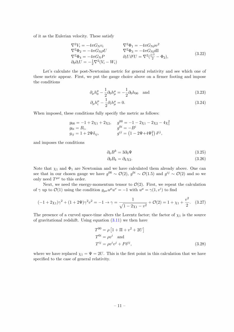
of it as the Eulerian velocity. These satisfy

∇2Vi = −4πGNvi ∇2Φ1 = −4πGNρv2

∇2Φ2 = −4πGNρU ∇2Φ3 = −4πGNρΠ

∇2Φ4 = −4πGNP ∂iU∂iU = ∇2(U

2

2 − Φ2),∂0∂iU = −1

2∇2(Vi −Wi)

(3.22)

Let’s calculate the post-Newtonian metric for general relativity and see which one ofthese metric appear. First, we put the gauge choice above on a firmer footing and imposethe conditions

∂µhµ0 −

1

2∂0h

µµ = −1

2∂0h00 and (3.23)

∂µhµi −

1

2∂ih

µµ = 0. (3.24)

When imposed, these conditions fully specify the metric as follows:

g00 = −1 + 2χ1 + 2χ2, g00 = −1− 2χ1 − 2χ2 − 4χ21

g0i = Bi, g0i = −Bi

gij = 1 + 2Ψδij , gij =(1− 2Ψ+4Ψ2

1

)δij ,

and imposes the conditions

∂kBk = 3∂0Ψ (3.25)

∂0Bk = ∂kχ2. (3.26)

Note that χ1 and Φ1 are Newtonian and we have calculated them already above. One cansee that in our chosen gauge we have g00 ∼ O(2), g0i ∼ O(1.5) and gij ∼ O(2) and so weonly need Tµν to this order.

Next, we need the energy-momentum tensor to O(2). First, we repeat the calculationof γ up to O(1) using the condition gµνu

µuν = −1 with uµ = γ(1, vi) to find

(−1 + 2χ1)γ2 + (1 + 2Ψ)γ2v2 = −1→ γ =1√

1− 2χ1 − v2+O(2) = 1 + χ1 +

v2

2. (3.27)

The presence of a curved space-time alters the Lorentz factor; the factor of χ1 is the sourceof gravitational redshift. Using equation (3.11) we then have

T 00 = ρ[1 + Π + v2 + 2U

]T 0i = ρvi and

T ij = ρvivj + Pδij , (3.28)

where we have replaced χ1 = Ψ = 2U . This is the first point in this calculation that we havespecified to the case of general relativity.

– 11 –

Exercise:

Show that:

T00 = ρ[1 + Π + v2 − 2U

](3.29)

T0i = −ρvivj (3.30)

Tij = ρvivj + Pδij and (3.31)

T = −ρ[1 + Π + v2

]+ ρv2 + 3P where T = gµνT

µν . (3.32)

Again, we want to use the trace-reversed Einstein equations. We’ll start with the 0i-component, which gives

∇2Bi + ∂i∂0U = 16πGNρvi. (3.33)

Using the identity (3.22), this becomes

∇2Bi = −∇2

(7

2Vi +

1

2Wi

)⇒ Bi = −7

2Vi −

1

2Wi. (3.34)

The 00-component gives

∇2(χ2 + U2 − 4Φ2) = ∇2 (2Φ1 − 2Φ2 + Φ3 + 3Φ4) (3.35)

and so one findsχ2 = −U2 + 2Φ1 + 2Φ2 + Φ3 + 3Φ4. (3.36)

Exercise:

If one expands gµν = ηµν + hµν show that:

R00 = −1

2∇2(h00 + 2U2 − 8Φ2) +O(3) (3.37)

R0i = ∇2h0i + ∂0∂iU +O(2.5) (3.38)

Rij = ∇2hij +O(2) (3.39)

(3.40)

You will need to use the O(1) solution h00 = hij = 2U and several of the identities given in(3.22) and (3.25) and (3.26).

Putting it all together, the post-Newtonian metric is

g00 = −1 + 2U − 2U2 + 4Φ1 + 4Φ2 + 2Φ3 + 3Φ4

g0i = −7

2Vi −

1

2Wi

gij = (1 + 2U)δij . (3.41)

– 12 –

This is the general relativity prediction for the geometry of space-time up to O(1/c4) outsidean isolated object. What we could do now is go ahead and try to calculate things likethe corrections to the properties of orbits or the bending of light, but, as we remarked inthe introduction, this is very cumbersome and there is a standard procedure for comparingexperimental measurements with theory once the metric has been found. Furthermore, thespecific form of the post-Newtonian metric (3.41) is not very enlightening; there are nospecific terms that correspond to individual new effects. For example, we all know thatgeneral relativity causes the perihelion of Mercury to precess but the rate of precession isnot linked to the presence of one term; several different terms contribute. This is made evenmore complicated by the fact that post-Newtonian corrections to the two-body problem areof a similar magnitude to the corrections coming from Newtonian sources such as the finitesize of the Sun and perturbations from other celestial objects such as Venus and the Earth.For this reason, we turn our attention to the generalised framework. This will allow us togain a better insight into the general relativity post-Newtonian metric; the terms that couldbe present but are not tell us a lot about the structure of gravity.

3.3 The Parametrised Post-Newtonian Framework

We can see that not all of the metric potentials that could be present in the metric actuallyappear in general relativity but there are many alternate theories where they might. Calcu-lating the 2PN metric in general relativity was straight-forward but any quick glance at atext book on post-Newtonian gravity reveals that translating this into the motion of celestialobjects is a long and cumbersome process. Rather than have to solve the two-body problemat 2PN for every theory of gravity, theorists in the 70’s and 80’s developed a parametrisedpost-Newtonian framework (PPN) for testing gravity in the solar system. The PPN metricin the gauge (3.23) and (3.24), which are known as quasi-Cartesian coordinates, is

g00 = −1 + 2U − 2βU2 − 2ξΦW + (2γPPN + 2 + α3 + ζ1 − 2ξ)Φ1 + 2(3γPPN − 2β + 1 + ζ2 + ξ)Φ2

+2(1 + ζ3)Φ3 + 2(3γPPN + 3ζ4 − 2ξ)Φ4 − (ζ1 − 2ξ)A− (α1 − α2 − α3)w2U − α2wiwjUij

+(2α3 − α1)wiVi, (3.42)

g0i = −1

2(4γPPN + 3 + α1 − α2 + ζ1 − 2ξ)Vi −

1

2(1 + α2 − ζ1 + 2ξ)Wi −

1

2(α1 − 2α2)wiU

−α2wjUij , (3.43)

gij = (1 + 2γPPNU)δij . (3.44)

This needs some explanation. First, note that all of the metric potentials (3.21) that we saidcould potentially appear in the metric are present. This is because we want to encompassas many theories of gravity as possible. The parameter γPPN was discussed above andparametrises deviations from general relativity in the Newtonian limit7. In particular, itdetermines the angle through which light is bent by the Sun. The other nine parameters β, ξ,αi and ζi parametrise deviations from general relativity. In particular, the case γPPN = β = 1,ξ = αi = ζi = 0 corresponds to the general relativity prediction we calculated above. Finally,there is the quantity wi. This is the velocity of the solar system relative to the mean restframe of the universe. This appears because there may be preferred frame effects in theoriesof gravity that include aethers or fixed external fields. These are parametrised by the αi

7It also appears in many post-Newtonian expressions, for example, the expression for the perihelion advanceof Mercury.

– 13 –

parameters, which are typically non-zero due to the effects of cosmological scalars and vectors.The PPN metric is written in this form rather than placing an arbitrary parameter in front ofeach metric potential so that each parameter carries a physical interpretation. I will outlinethis briefly below:

• γPPN — The amount of spacial curvature produced per unit rest mass. This alters themotion of light relative to non-relativistic particles.

• β — The amount of non-linearity in the superposition law for gravity. This affects themotion of binary objects, for example, it causes a periodic shift in the perihelion ofMercury.

• ξ — The Whitehead parameter. General relativity requires one to solve for the metricbefore solving for the motion of particles. Alfred North Whitehead saw this as acausaland introduced a new theory in 1922 where the physical metric seen by particles onlydepends on quantities evaluated along their past light-cone. The theory makes iden-tical predictions to general relativity except that ξ = 1 and passes all of the classicaltests including light bending and the perihelion shift of mercury. It remained a viablecompetitor to general relativity until 1971 when it was pointed out that when ξ 6= 0there are anisotropies in the local value of GN in three-body systems. This results inlarge unobserved tides on Earth due to the motion of the solar system through theMilky Way. ξ is zero in the majority of alternate theories of gravity but is non-zero inquasi-linear theories.

• α1 and α2 — These describe preferred frame effects. They are typically zero unlessthe theory violates Lorentz invariance or contains some sort of aether. Theories withnon-zero cosmological vectors typically act as an aether.

• ζi — These are the so-called conservation law parameters. When they are non-zero,the theory lacks the conservation laws that usually arise due to translational invariancesuch as energy and momentum conservation.

• α3 — This is both a preferred frame and conservation law parameter.

Not only do these parameters tell us about deviations from general relativity but they also tellus about conservation laws. Recall that the Poincare group (Lorentz group + translations)group has 10 conserved currents Pµ, the energy and momentum and Jµν , the angular mo-mentum. It turns out that these are only conserved in a curved space if certain combinationsof the parameters are zero. There are three classes of theories

1. Conservative theories: These have αi = ζi = 0 and conserve both Pµ and Jµν .

2. Semi-Conservative theories: These have ζi = α3 = 0 and either α1 or α2 non-zero. Inthis case Pµ is conserved but Jµν is not.

3. Non-Conservative theories: These have one of ζi or α3 non-zero and do not conserveany quantities.

There is a theorem that any theory that can be derived from a diffeomorphism-invariantLagrangian is at least semi-conservative. We end this section by presenting the currentbounds on the PPN parameters in table 3.3.

– 14 –

Parameter Constraint Experiment

γPPN − 1 2.5× 10−5 Light bending by the Sun measured by the Cassini probeβ − 1 3× 10−3 Perihelion shift of Mercuryξ 10−3 Gravimetric data about the Earth’s tidesα1 10−4 Orbit polarisation measured using Lunar Laser Rangingα2 4× 10−7 Spin precession of the Sun’s axis with respect to its eclipticα3 4× 10−20 Pulsar spin-down statisticsζ1 0.02 Combined PPN boundsζ2 4× 10−5 Binary pulsar accelerationζ3 10−8 Newton’s third law measured using the acceleration of the Moonζ4 0.4 Difference in active and passive mass between bromine and fluorine.

3.3.1 The PPN Metric for Scalar-Tensor Theories

As an example of how to apply the PPN formalism, let’s look at one of these alternate theoriesI keep talking about: scalar-tensor theories. These theories include a new scalar field φ andare described by the action

S =

∫ √−g 1

16πG

[R

2− 1

2∂µφ∂

µφ

]+ Sm[gµν ]. (3.45)

The metric that couples to matter is not the Einstein frame metric gµν but instead it is theJordan frame metric

gµν = A2(φ)gµν . (3.46)

One very common choice of coupling function is

A(φ) = eαφ, (3.47)

where α is a constant. The equations for the tensor gµν are simply the Einstein equationssourced by both matter and the scalar

Gµν = 8πG (Tµν + Tφ, µν) (3.48)

where

Tφ, µν =1

8πG

(∂µφ∂νφ−

1

2∂µφ∂

µφgµν

). (3.49)

Note that I have used G ≡ (8πMpl2)−1 here and not GN. It is often the case in alternate

theories of gravity that what you call G in the action is not the same thing as GN, the locallymeasured value of Newton’s constant, and so it is best to distinguish between the two. Onealso needs the scalar field’s equation of motion, which is

φ = −8πGTd lnA

dφ, (3.50)

where = gµν∇µ∇ν . Since it is the Jordan frame metric that couples to matter we need tocompute this in the same manner that we did before. The added complication is the scalar.We will make the ansatz that φ = φ0 +φ1 +φ2 where φ0 is the cosmological value of the field,φ1 ∼ O(1) is the Newtonian field (1PN) and φ2 ∼ O(2) is the post-Newtonian field (2PN).

– 15 –

We will set φ0 = 0 so that A(φ0) = 18. Note then that the Jordan frame metric is, to theappropriate order,

g00 =(−1 + 2[χ1 − αφ1] +

[2χ2 + 2αφ2 + α2φ2

1

])g0i = Bi

gij = (1 + 2Ψ + 2αφ1)δij , (3.51)

where the metric potentials have been defined in the Einstein frame according to (3.25).In particular, the g00 component at O(1) is χ1 − αφ1 and so we have an effective value ofχ1 = χ1 − αφ1. This means that in the Jordan frame, the energy-momentum tensor is givenby (3.28) with χ1 → χ1. The only complication here is that the energy-momentum tensorsin the different frames are related via

Tµν = A6(φ)Tµν . (3.52)

The physical quantities such as the coordinate velocity, the density and pressure etc. shouldbe defined in this frame since it is the frame in which gravity is minimally coupled andone has ∇µTµν = 0. ∇µTµν 6= 0 in the Einstein frame since the scalar couples to matterand instead we have ∇µ(Tµν + Tµνφ ) = 0. It turns out that at the post-Newtonian levelthis, theory is indistinguishable from general relativity and that the only change is at theNewtonian level. For this reason, I will only calculate the Jordan frame metric to O(1). Tothis order, Tµν = Tµν and so we can use all of the formulae given in the previous sectionprovided that we work to O(1) only. Also, we do not need to worry about Tφ ,µν . The reasonis the following: expanding it out around the cosmological field value φ0 to O(1) one finds

T 00φ = 0

T 0iφ = −φ0

T ijφ = 0. (3.53)

The only non-zero term is in T ij and this is multiplied by φ0. Since φ0 is a cosmologicalscalar we expect φ0 ∼ H0φ0 ∂ihµν and so one can ignore the scalar’s contribution to theenergy-momentum tensor. This is an important feature of alternate theories of gravity, thelocal space-time curvature should be sourced by the matter and not the scalar. With thissimplification, at O(1) the Einstein equations are identical to general relativity and so onehas

χ1 = Ψ = U, (3.54)

with the caveat that U is defined using G and not GN. We will return to this later. Nowlet’s solve for the scalar. To O(1) we have T = −ρ and so equation (3.50) is

∇2φ1 = 8απGρ⇒ φ1 = −2αU. (3.55)

This is all we need to solve for the O(1) metric. Putting the solutions for χ1, Ψ and φ1 intothe Jordan frame metric (3.51) we have

g00 = −1 + 2U(1 + 2α2)

g0i = 0

8We can always rescale the Jordan frame coordinates at zeroth-order so that this is the case.

– 16 –

gij =[1 +

(1− 2α2

)U]δij . (3.56)

This is not in the PPN form because the coefficient of U in g00 6= 1 (see (3.42)). This isbecause what we called G in the action is not the same as GN. Since U contains a factor ofG we can define GN ≡ (1 + 2α2)G, in which case we have

g00 = −1 + 2U

g0i = 0

gij =

[1 + 2U

(1− 2α2

1 + 2α2

)]δij , (3.57)

where U is now defined using GN. Comparing with (3.44), we see that this is now in PPNform with

|γPPN − 1| = 4α2

1 + 2α2. (3.58)

Now comes the power of the PPN formalism: Rather than deriving the effects of γ 6= 1 on themotion of light and particles we know that the strongest constraint on its value in a metricof the PPN form comes from the Cassini probe, which constrains this quantity to be smallerthan 10−5. This imposes the constraint

4α2 <∼ 10−5. (3.59)

Scalar-tensor theories are highly constrained.

Exercise:

More general scalar-tensor theories can be parametrised as follows:

lnA(φ) = α0(φ− φ0) +1

2β0(φ− φ0)2 + . . . . (3.60)

Using this parametrisation, calculate the Jordan frame metric to 2PN order and show that

γPPN =1− 2α2

0

1 + 2α20

, β =α2

0β0

2(1 + 2α2)2, αi = ζi = ξ = 0. (3.61)

You will need to make sure you scale G by the appropriate factors of α0 when you convertto GN.

4 Screening Mechanisms

Many people who study alternate theories of gravity are interested in the cosmological con-stant problem and looking for accelerating solutions but there is no way that a theory likethe one that we studied above can possibly have any major effect on the expansion of theuniverse if the only new parameter α is five orders-of-magnitude smaller than unity. Theproblem with many alternate theories of gravity is that solar system tests are so strong thatthey render the theory irrelevant on all scales. What would be nice if there was some sortof mechanism where the scalar’s effects are negligible in the solar system but important forcosmology. To see if this is possible, let’s look at what went wrong above. Written in theEinstein frame, the theory looked like Einstein’s equations plus an extra equation for the

– 17 –

scalar. When written in the Jordan frame, we found that the metric potential χ1, whichgoverns non-relativistic geodesics, was related to the Einstein frame potentials via

χ1 = χ1 − 2αφ1. (4.1)

Now χ1 satisfied the Poisson equation of general relativity

∇2χ1 = −4πGρ⇒ χ1 = 2U (4.2)

but so did the scalar up to a factor of −2α:

∇2φ1 = 8πGαρ⇒ φ1 = −2αχ1. (4.3)

When put together, this meansχ1 = (1 + 2α2)χGR

1 . (4.4)

This means that observers making measurements with respect to the Einstein frame metricsee a value of GN = (1 + 2α2)G. Screening mechanisms attempt to hide modifications ofgeneral relativity by changing the Poisson equation for φ such that the solution is verydifferent from U . When written in the Einstein frame, the theory looks like one with agravitational- and an additional fifth-force

~FN = −∇U, ~F5 = −α∇φ, (4.5)

and so the solution of the new Poisson equation should satisfy α|∇φ|/|∇U | 1 in theEinstein frame. There are two very different approaches to this. One is to somehow killof the source for the Poisson equation so that no scalar gradients are generated by massiveobjects, and the other is to change the derivative interactions on the left hand side so thatthe solution is very different from U . In this lecture we will examine both of these. Fromhere on I will change notation from φ1 to φ. The reason for this is that screening mechanismstend to be non-linear in the field equations and it does not make sense to split them up intoPPN orders any more.

4.1 Killing off the Source

Killing off the source on the right hand side of the Poisson equation is the method used bychameleon and symmetron theories. This is achieved by adding a scalar potential to theaction so that it is now

S =

∫d4x√−g 1

8πG

[R

2− 1

2∇µφ∇µφ− V (φ)

]+ Sm[A2(φ)gµν ]. (4.6)

In this case, the Einstein equations are still the same and we can still ignore the scalar’scontribution to the energy-momentum tensor but the scalar’s equation is modified to

φ = −8πGTd lnA

dφ+ V ′(φ) = V ′(φ) + 8πG

d lnA

dφρ. (4.7)

The right hand side looks like an effective potential for the scalar:

Veff = V (φ) + ρ lnA (4.8)

– 18 –

Figure 2. A spherical gravitational source. The entire object sources the gravitational fields χ1 andΨ but only the mass in the shell sources the scalar φ.

and we can use this to our advantage. The idea is the following. Suppose we choose V (φ)and A(φ) such that Veff(φ) has a minimum at some φmin. φmin depends on ρ and so theminimum inside objects will be different from the minimum in the cosmological background.This means that inside the object, the field will want to move to reach the value φmin(ρ).Since φmin(ρ) is the solution of V ′eff(φmin) = 0, the field equation is simply

∇2φ = 0. (4.9)

The equation for the field is unsourced and there is no scalar gradient and hence fifth-force. Atsome point, the field will have to move away from the minimum and towards its cosmologicalvalue and we expect some intermediate scale where we have fifth-forces. The essence of thescreening mechanism is that it is possible to find parameters where this only happens in avery narrow shell near the surface. In this case, the field outside is only sourced by this verythin shell and the fifth-force is very heavily suppressed. This is shown schematically in figure2.

Let’s see how this works in practice. We start by defining a parameter α similar to theone above via

α ≡ d lnA

dφ

∣∣∣∣φ=φ0

(4.10)

and restrict to the case of spherical symmetry. We split the object into two regions separatedby some screening radius rs shown in figure 2. When r < rs the field minimises its potentialso that φ = φmin. There is no source for the field in this region and φ′ = 0. Outside, equation(4.7) becomes

∇2φ = V ′(φ) + 8παGρ r > rs (4.11)

Let’s make the further assumption that V ′(φ) can be neglected with r > rs. This is avalid assumption because V ′(φ) ≈ m2

0φ, where m20 = V ′′(φ0) is the mass of the field in the

cosmological background. This is typically of order H−20 whereas ∇2φ ∼ φ/R2, where R is

the radius of the object and so the mass term is negligible compared with the Laplacian. Inthis case, the equation of motion reduces to

1

r2

d

dr

(r2 dφ

dr

)= 8παGρ r > rs. (4.12)

This can easily be integrated using the fact that the mass enclosed inside a radius r is

M(r) = 4π

∫r2ρ(r) dr (4.13)

– 19 –

Object ΦN

Earth 10−9

The Sun 2× 10−6

Main-sequence stars 10−6–10−5

Local group 10−4

Milky Way O(10−6)Spiral and elliptical galaxies 10−6–10−5

Post-main-sequence stars 10−7–10−8

Dwarf galaxies O(10−8)

Table 1. The Newtonian potential of different astrophysical objects.

to find

F5 = αdφ

dr= 2α2GM

r2

[1− M(rs)

M(r)

]r > rs. (4.14)

The familiar factor of 2α2 is still there but now it is multiplied by a factor of

Q ≡[1− M(rs)

M(r)

]. (4.15)

When the screening radius is close to the radius of the object, R ,we have M(rs) ≈M , whereM ≡M(R) is the total mass of the object and so Q 1. In this case the object is screened.In the opposite limit where rs = 0 we have Q = 1 and the fifth-force is a factor of 2α2 largerthan the Newtonian one. In this case the object is unscreened. We will not show it here butthe the screening radius is determined by the self-screening parameter9

χ0 ≡φ0

2α. (4.16)

In particular the screening radius is determined implicitly through the relation

χ0 = 4πG

∫ R

rs

rρ(r) dr. (4.17)

When dealing with objects of mass M and radius R a good rule of thumb to determinewhether they are screened or not is:

• If χ0 < GM/R the object is self-screening

• If χ0 > GM/R the object is at least partially unscreened.

This is a good criterion to use when deciding if a certain astrophysical system will be un-screened or not and gives us a good idea of where to test these theories. Note that for theSun and the Milky Way GM/R ∼ 10−6 and so χ0 < 10−6 is a rough constraint found byrequiring that they are screened. Dwarf galaxies have GM/R ∼ 10−8 and so a lot of efforthas been focused on looking at these systems as potential probes. The Newtonian potentialsof some useful astrophysical objects are given in table 4.1.

9Technically, objects can be screened by their neighbours but we will not deal with this complication here.

– 20 –

Now let’s go back and look at the solution outside the object, which is

χ1 = Ψ =GM

r(4.18)

αφ = −Q(R)GM

r, (4.19)

where Q(R) = 1−M(rs)/M . This gives the Jordan frame metric to 1PN as

g00 = −1 + 2U (1 +Q) (4.20)

g0i = 0 (4.21)

gij = [1 + 2U (1−Q)] δij . (4.22)

Setting GN = (1 +Q)G we can bring this into PPN form with

γPPN =1−Q1 +Q

. (4.23)

The difference now is that α can in principle be large because Q 1 (provided χ0 < 10−6).This means that this theory has no trouble passing the Cassini bound and it is still possibleto have interesting effects on cosmological scales.

4.1.1 Two Examples: The Chameleon Mechanism

The first example of a theory that utilised this mechanism was chameleon screening. Thecoupling function and scalar potential are

V (φ) =M4+n

φn, A(φ) = eαφ, (4.24)

with α constant. The effective potential is then

Veff(φ) =M2

φn+ 8παGρ, (4.25)

which has a density-dependent minimum at

φ(ρ) =

(nM2

8παGρ

) 1n+1

. (4.26)

This is shown in figure 3. One can see that this potential has all of the properties that weneed: If we consider a spherical over-dense object then the effective potential will have twominima, one inside the object and one inside the low-density background. Furthermore, theeffective mass at the minimum is

m2eff = V ′′eff(φmin) = n(n+ 1)M2

(8παGρ

nM

)n+2n+1

. (4.27)

This is an increasing function of density and so the mass at the high density minimum can beseveral orders-of-magnitude larger than the mass at the low density minimum. Recall thatthe force-law for a massive scalar is of the Yukawa form

F ∝ e−meffr

r2. (4.28)

– 21 –

Figure 3. The effective potential for chameleon screening. The left panel shows the effective potentialin low-desnity environments and the right shows the same potential in high-density environments. TheBlack dashed line shows the scalar potential V (φ) and the red dotted line shows the coupling functionρeαφ. The effective potential, which is the sum of the two, corresponds to the blue solid line.

In practice, the parameter M is chosen such that meff<∼ O(µ m) so that the fifth-force

operates over ranges shorter than the most precise table-top experiments can probe. The non-linear field equation for the scalar opens up exciting possibilities of searching for chameleonsusing laboratory experiments with different geometries and densities but this is beyond thescope of these notes.

Before moving on, let’s look at a very popular class of models: F (R) theories. It turnsout that these are chameleons in disguise. The action for these theories is

S =

∫d4x√−g f(R)

16πG+ Sm[gµν ], (4.29)

where R = R(g). One can write this in an equivalent way using a new variable ψ:

S =

∫d4x

√−g

16πG

[f(ψ) + f ′(ψ)(R− ψ)

]+ Sm[gµν ]. (4.30)

If f ′′(ψ) 6= 0 the equation of motion for ψ is ψ = R, which can be put back into the actionto recover (4.29). Next, we set Φ = f ′(ψ) to find

S =

∫d4x

√−g

16πG[ΦR− V (φ)] + Sm[gµν ], (4.31)

whereV (Φ) = ψ(Φ)Φ− f(ψ(Φ)). (4.32)

Finally, setting Φ = e−√

23φ

and applying a Weyl rescaling to gµν such that gµν = A2(φ)gµν

with A(φ) = eφ√6 one finds (after removing a total derivative proportional to φ)

S =

∫d4x

√−g

8πG

[R(g)

2− 1

2∇µφ∇µφ− V (φ)

]+ Sm[A2(φ)gµν ], (4.33)

with

V (φ) =Rf ′(R)− f(R)

2f ′(R)2. (4.34)

– 22 –

Provided one chooses f(R) such that V (φ) is of the chameleon form then the theory is achameleon with α = 1/

√6. f(R) theories are very popular in the literature because the

coupling α is fixed and so there is only one free parameter: χ0. In the language of f(R)theories, people often work with the parameter fR0 = f ′(R) evaluated at the present timein the cosmological background. In terms of χ0, one has χ0 = 3/2fR0. The most commonexample of an f(R) theory that exhibits chameleon screening is the Hu & Sawicki model:

f(R) = R−m2 c1(R/m2)n

1 + c2(R/m2)n. (4.35)

Exercise:

Consider the Weyl rescaling:

gµν = A2(φ)gµν . (4.36)

Show that: √−g = A4(φ)

√−g (4.37)

R(g) = A−2 [R(g)− 6ω − 6gµν∇µω∇νω] , (4.38)

with ω = lnA. Use this to transform equation (4.31) into equation (4.33). You will findWald, appendix D useful.

4.1.2 Two Examples: The Symmetron Effect

The symmetron is described by the potential and coupling function

V (φ) = −µ2φ2

2+ λ

φ4

8πG, A(φ) = 1 +

αφ2

2(4.39)

so that the effective potential is of the Z2-symmetry breaking form

Veff(φ) =µ2

2

(8παGρ

µ2− 1

)φ2 + λ

φ4

8πG=µ2

2

(ρ

ρ?− 1

)φ2 + λ

φ4

8πG, (4.40)

with ρ? = µ2/8παG. This is plotted in figure 4 for both ρ > ρ? and ρ < ρ?. One cansee that when ρ < ρ? the Z2 symmetry is broken and the potential has a minimum atφ± ≈ ±µ

√2πG/λ. When ρ > ρ? the symmetry is restored and the only minimum lies at

φ = 0. We want to screen inside high-density objects and so one typically chooses the modelparameters such that ρ? lies between the cosmological density ρc ∼ 3H2

0Mpl2Ωm0 and the

central density of the object in question. When this is the case, the theory has all of thefeatures we want: there are two distinct density-dependent minima. That being said, thescreening mechanism is very different from the chameleon mechanism we saw above. In orderto screen at sub-cosmological densities we require µ2 <∼ H2

0 . The effective mass of the field isthen meff ∼ µ <∼ H0 and so the field is always very light. Instead of altering the range of theforce, the symmetron screens the force because the coupling α(φ) ≈ 0. The fifth-force (4.5)is

~F5 = −α(φ)∇φ ≈ αφ∇φ. (4.41)

Provided the field has reached its symmetry restoring minimum i.e. φ = 0 this is identicallyzero.

– 23 –

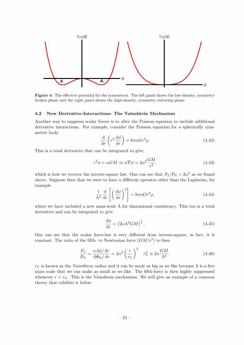
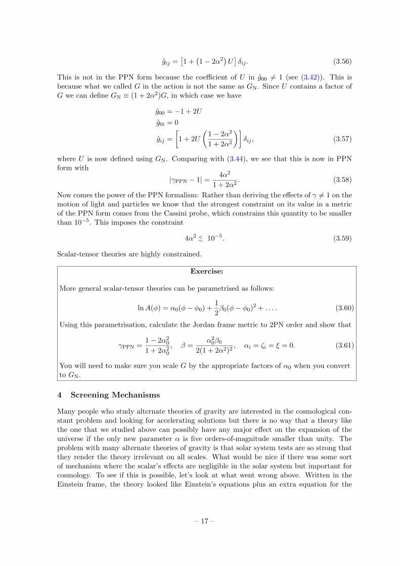
Figure 4. The effective potential for the symmetron. The left panel shows the low-density, symmetrybroken phase and the right panel shows the high-density, symmetry restoring phase.

4.2 New Derivative-Interactions: The Vainshtein Mechanism

Another way to suppress scalar forces is to alter the Poisson equation to include additionalderivative interactions. For example, consider the Poisson equation for a spherically sym-metric body

d

dr

(r2 dφ

dr

)= 8παGr2ρ. (4.42)

This is a total derivative that can be integrated to give,

r2φ = αGM ⇒ α∇φ = 2α2GM

r2(4.43)

which is how we recover the inverse-square law. One can see that F5/FN = 2α2 as we foundabove. Suppose then that we were to have a different operator other than the Laplacian, forexample

1

Λ4

d

dr

[(dφ

dr

)3]

= 8παGr2ρ, (4.44)

where we have included a new mass-scale Λ for dimensional consistency. This too is a totalderivative and can be integrated to give

dφ

dr=(2αΛ4GM

) 13 . (4.45)

One can see that the scalar force-law is very different from inverse-square, in fact, it isconstant. The ratio of the fifth- to Newtonian force (GM/r2) is then

F5

FN=α dφ/ dr

dΦN/ dr= 2α2

(r

rV

)2

r3V ≡ 2α

GM

Λ2. (4.46)

rV is known as the Vainshtein radius and it can be made as big as we like because Λ is a freemass scale that we can make as small as we like. The fifth-force is then highly suppressedwhenever r < rV. This is the Vainshtein mechanism. We will give an example of a commontheory that exhibits it below.

– 24 –

4.2.1 Example: Cubic Galileons

Galileon theories have received a lot of theoretical attention lately due to their links withmassive gravity and powerful non-renormalisation theorems. Here, we are only interestedin their small-scale behaviour. Galileon theories are invariant under the galileon symmetryφ → φ + bµx

µ + c when expanded around Minkowski space and it turns out there are fourpossible derivative operators that one can write down in four dimensions. The simplest isthe cubic galileon:

S =

∫d4x

√−g

8πG

[R

2− 1

2∂µφ∂

µφ− 1

Λ2∂µφ∂

µφφ

]+ Sm[gµν ], gµν = e2αφgµν . (4.47)

The name cubic galileon derives from the fact that the new operator action contains theefields. Similarly, there are quartic and quintic galileons. Despite being higher-order, thegalileon shift symmetry ensures that the equations of motion are second-order and the theoryis therefore free of the Ostrogradski ghost instability. Since we are working in the Einsteinframe, the equations of motion for the metric are Einstein’s equations and the scalar equationof motion is

φ+2

Λ2

[(φ)2 −∇µ∇νφ∇µ∇νφ

]= 8παGρ. (4.48)

In the case of a static spherically symmetric configuration this becomes

1

r2

d

dr

[r2 dφ

dr+

r

Λ2

(dφ

dr

)2]

= 8παGρ. (4.49)

We can recognise the first term as the usual contribution from the Laplacian. The secondterm is the new contribution from the cubic galileon operator. This can be integrated onceto give

dφ

dr+

1

Λ2r

(dφ

dr

)2

= 2αGM

r2. (4.50)

Note that the right hand side is 2α times the Newtonian force and so we can begin to seethe Vainshtein mechanism at work. In the absence of the cubic galileon we are back to thecase studied above where F5 = 2α2FN, but the presence of the galileon term changes this.One can already see that the second term dominates at small distances but let’s put this ona more concrete footing. Introducing the Vainshtein radius

r3V =

GM

αΛ2(4.51)

and setting dφ/dr = F5/α we can divide by FN = GM/r2 to find

F5

FN+(rV

r

)3(F5

FN

)2

= 2α2. (4.52)

One can then see the Vainshtein mechanism at work. When r rV the new term dominatesover the Laplacian and we have

F5

FN= 2α2

(r

rV

) 32

(4.53)

whereas when r rV the new term is suppressed and we recover the inverse-square be-haviour. This is shown in figure figure 5.

– 25 –

Figure 5. Vainshtein screening of a spherical object.

Exercise:

Use equation (4.48) to derive equation (4.49). The Christoffel symbols are not zero, despitethe fact that we are working in a flat space-time and you will need to use this.

Whether or not an object screens then depends on the Vainshtein radius. Lunar LaserRanging measures the motion of the Moon about the Earth very precisely and constrainsdeviations in the gravitational potential:

δΦN

ΦN< 2.4× 1011. (4.54)

Using equation (4.53) we have

δΦN

ΦN= 2α2

(r

rV

) 32

. (4.55)

The Earth-Moon distance is 3.84× 108 m and so one finds r⊕V > 7.3× 1015m ∼ O(10−1) Pcfor α = 1. Now note that

r3V =

rS

Λ2, (4.56)

where rS is the Schwarzchild radius. This is 9 mm for the earth and so one has Λ2 =2.3× 10−53 mm−2 if we assume the LLR bound is just satisfied. The Schrwazchild radius ofthe Sun is ∼ 3 km and so we find rV ∼ O(pc). The Vainshtein radius of the Sun is largerthan the solar system. One can see that Vainshtein screening is incredibly efficient. This isboth a blessing and a curse: deviations from general relativity are well hidden but findingnovel probes of the mechanism is incredibly difficult.

– 26 –

4.3 Equivalence Principle Violations

We end this chapter by discussing the most important difference between the two screeningmechanisms: violations of the equivalence principle. General relativity was founded on theequivalence principle: The motion of test-bodies is independent of their structure and com-position. This appears in the Newtonian limit of general relativity as follows. We know thatthe geodesic equation gives us the force-law

M~x = −M∇ΦextN (4.57)

in the non-relativistic limit. Here, ΦextN refers to the Newtonian potential generated by some

external body e.g. the Sun. The mass on the left-hand side is the inertial mass, it is themass we put into the point-particle action

S = −M∫

ds√−gµν xµxν , (4.58)

where in this one instance a dot denotes a derivative with respect to the proper time s. Themass on the right hand side is the gravitational mass. This should be thought of more as agravitational charge in analogy with electromagnetism. It tells us how strongly a test-bodyresponds to an external gravitational field Φext

N . The fact that MLHS = MRHS means thatthey cancel and the motion of a non-relativistic particle is independent of its mass. This isthe equivalence principle. In scalar-tensor theories, (4.57) is generalised to

M~x = −M∇ΦextN −Q∇φext, (4.59)

where Q is the scalar gravitational charge. One can see that if Q = M or Q = 0 theequivalence principle is satisfied. Deriving the value of Q in these theories is a long andcumbersome process and so rather than provide a hand-wavy, incorrect proof, I will simplystate the results here:

Q = M[1− M(rs)

M

], Chameleons

Q = M Vainshtein.(4.60)

Chameleon-like theories do not satisfy the equivalence principle because Q 6= M unlessthe screening radius is zero or equal to the radius of the object i.e. unless the object isfully screened or fully unscreened. Theories that screen using the Vainshtein mechanism dosatisfy the equivalence principle10. The equivalence principle is very well tested in the solarsystem and this allows one to constrain chameleon theories but not those that screen usingthe Vainshtein mechanism.

5 Non-Relativistic Stars: A Laboratory for Testing Fundamental Physics

In this final chapter, we will look at the structure of non-relativistic stars and see how theycan be used to test alternate theories of gravity.

10The one exception to this is black holes but we are not interested in highly relativistic objects here.

– 27 –

5.1 Stellar Structure Equations

We begin by deriving the equations of stellar structure. Non-relativistic stars are spherical toa good approximation and, we can treat them as a perfect fluid described by their Eulerianpressure P and density ρ. Working in the rest-frame of the star, we have γ = 1 and souµ = (1,~0). The energy momentum tensor (3.11) is then

Tµν = diag(ρ, P, P, P ). (5.1)

The space-time isds2 = −(1− 2Φ) dt2 + (1 + 2Ψ)δij dxi dxj . (5.2)

The equation of motion for the fluid is given by the zero-component of

∇µTµν = 0, (5.3)

which results indΦ

dr= −1

ρ

dP

dr. (5.4)

Note that we have not specified the theory of gravity, all we have done is assume that Tµν isconserved, which means we are working in the Jordan frame. The theory of gravity determinesdΦ/ dr so let’s specialise to general relativity for now and set dΦ/dr = GM(r)/r2. Thisgives us the hydrostatic equilibrium equation:

dP

dr= −GM(r)ρ(r)

r2. (5.5)

We also have an equation for M(r):

dM(r)

dr= 4πGr2ρ(r) (5.6)

but this does not close the system of equations and allow us to solve for P (r) and ρ(r). Inorder to do this we must specify non-gravitational physics. First, we know that in order tosupport themselves against gravitational collapse, stars must burn fuel in their centres. If εiis the energy released per unit mass from the ith burning process in the core and εi is theenergy lost in that process (e.g. from neutrinos produced in the reactions, that stream away)then the luminosity, the energy released per unit time, is given by

dL(r)

dt= 4πr2ρ(r)

(∑i

εi −∑i

εi

). (5.7)

This is the energy generation equation. The surface luminosity L ≡ L(R) is one of the mostimportant stellar parameters since it is directly observable. Another observable quantity isthe effective temperature Teff . The temperature gradient in a star is given by the radiativetransport equation

dT

dr= − 3

4a

κ(ρ, T )

T 3

ρL

4πr2. (5.8)

Here a is a constant that appears in the pressure law for radiation (we will see this explicitlyin a moment) and κ(ρ, T ) is the opacity (the cross-section for radiation absorption per unitmass). These equations still do not close as one needs to supply equations of state of the

– 28 –

form κ(ρ, T ), P (ρ, T ) and εi = εi(ρ, T ). In practice, complicated numerical codes are neededto solve these problems but there are several simplifying assumptions one can make in orderto gain valuable physical insights. The pressure in most stars is primarily due to the internalmotions of the gas particles as described by the idea gas law:

Pgas =ρkBT

µmH, (5.9)

where µ is the mean molecular mass and mH is the mass of Hydrogen, and the pressure dueto absorbing radiation in the interior:

Prad =1

3aT 4. (5.10)

In what follows we will consider these pressure laws only. Furthermore, to avoid dealing withatmospheric models we will define the radius of the star R as the radius where the pressurefalls to zero i.e. P (r) = 0.

5.2 Scale-Invariance of the Stellar Structure Equations

One can make a lot of progress by noting that the stellar structure equations are scale-invariant. To see this, consider the hydrostatic equilibrium equation (5.5). Since P has unitsof GM/r4 we can see that if one scales P → PcxP , where Pc is the central pressure, r → Rxr,M(r)→MxM and ρ(r)→ xρM/R3, where xi are dimensionless functions we have

PcdxPdxr

= −GM2

R4

xρxMx2r

. (5.11)

Now since xi are dimensionless we can immediately see that

Pc ∝GM2

R4. (5.12)

We have a relation for how Pc scales with G, M and R without having to have solved anyequations. Let’s see how far we can push this. Doing the same thing for the radiative transferequation we find

L ∝ R4T 4

M. (5.13)

Now we need to decide what our equation of state is. If we assume that the star is gasdominated we find

P ∝ MT

R3⇒ T =

GM

R(5.14)

using equation (5.9) and (5.12). If we instead assume it is radiation dominated we have, fromequation (5.10) and (5.12)

P ∝ T 4. (5.15)

Inserting these into equation (5.13) we have

L ∝ G4M3 gasL ∝ GM radiation.

(5.16)

This gives us a mass-luminosity relation and shows us how the luminosity scales with thestrength of gravity. One can see that gas-supported stars are more sensitive to changes in G

– 29 –

than radiation-supported stars. Furthermore, theories of gravity that predict stronger gravitythan general relativity predict that stars are more luminous whilst the converse is true fortheories that predict weaker gravity. Physically, this is because stronger gravity means fuelmust be burnt at a higher rate to provide the extra pressure gradient needed to stave offgravitational collapse and hence the rate of energy release increases. Using equation (5.9)and (5.10) one finds

Prad

Pgas∝ T 3

ρ∝ G3M2 (5.17)

and so one can see that low mass stars are gas-supported and high mass stars are radiation-supported. Low mass stars are therefore a better probe of modified gravity11. One can alsosee that increasing G makes stars more radiation supported at fixed mass.

5.3 Ploytropic Equations of State: The Lane-Emden Equation

One of the simplest choices for the equation of state is

P = Kρn+1n . (5.18)

This is known as a polytropic equation of state and n is known as the polytropic index.Polytropes are very important in stellar physics and can describe a variety of different stars.For example, n = 3 describes low mass main-sequence stars and fully relativistic (whitedwarf) stars, n = 1.5 describes fully convective stars and n = 5 can be used to modelglobular clusters. Let’s see what happens to the stellar structure equations if we assume thisequation of state. First, we define a few important quantities. Since the stellar structureequations are scale invariant12 we can reduce the system to dimensionless form. First, wedefine the dimensionless radial coordinate ξ via:

r = r0ξ, r20 =

(n+ 1)Pc

4πGρ2c

, (5.19)

where a c refers to central quantities. Since the stellar radius is defined as the point whereP (R) = 0 it is useful to define ξR via θ(ξR) = 0. The stellar radius is then R = r0ξR. Wealso define the dimensionless function θ(ξ) via

P = Pcθn+1

ρ = ρcθn. (5.20)

This gives us the relation Pc = Kρn+1n

c . Dividing equation (5.5) by Gρ/r2 we have

r2

Gρ

dP

dr= −M(r), (5.21)

which can be differentiated once using equation (5.6) to find

1

r

d

dr

(r2

4πGρ

dP

dr

)= −ρ(r). (5.22)

11Provided of course that one is trying to test it using the stellar luminosity.12Actually, the symmetry is even larger than this. The stellar structure equations with a polytropic equation

of state are homology-invariant. This means that once you know one solution with one boundary conditionyou actually know other solutions with different boundary conditions. This goes beyond the scope of thecourse but it allows one to analyse the equations using very powerful mathematical techniques.

– 30 –

Inserting the equation of state (5.18) and changing to dimensionless variables using (5.19)and (5.20) we arrive at the famous Lane-Emden equation

1

ξ2

d

dξ

(ξ2 dθ

dξ

)= −θn. (5.23)

This equation is non-linear and can only be solved in a few special cases, all of which areuninteresting for testing gravity. These are given in box 1 for completeness. In practiceone needs to solve this numerically but this is simple and can be done using elementarytechniques such as the Runge-Kutta family of methods. We still need to specify the boundaryconditions. We know that the central pressure is given by Pc and so we clearly have θ(0) = 1.The second boundary condition is forced on us by spherical symmetry: the pressure mustgo to zero smoothly at r = 0 and so we have θ′(0) = 0. Some examples of the solutionssatisfying these conditions are shown in figure 6. With these conditions, one can show thatthe behaviour of θ near the origin is

θ(ξ) = 1− ξ2

6+

n

120ξ4. (5.24)

This is useful when integrating the equations numerically because one cannot typically spec-ify the boundary condition at ξ = 0 but instead must integrate from ξ = δ where δ 1.

Box 1: Exact solutions of the Lane-Emden equation

n = 0 : θ(ξ) = C0 − C1ξ −

16ξ

2

n = 1 : θ(ξ) = C0sin ξξ + C1

cos ξξ

n = 5 : θ(ξ) = 1√1+ξ2/3

,(5.25)

where Ci are integration constants.

5.3.1 The Mass Radius Relation and the Chandrasekhar Mass

Typically, we cannot see inside stars and so, in some sense, Pc and ρc are meaningless quan-tities. What we observe are quantities such as the mass, radius and luminosity. Polytropicequations of state predict a mass-radius relation that we will derive here. First, we canintegrate equation (5.6) to give

M =

∫ R

04πr2ρ(r) dξ = 4πr3

0ρc

∫ ξR

0ξ2θn(ξ) dξ = −4πr3

0ρc

∫ ξR

0

d

dξ

(ξ2 dθ

dξ

)= 4πωRr

30ρc, (5.26)

where we have used the Lane-Emden equation to replace θn and have defined

ωR ≡ −ξ2R

dθ

dξ

∣∣∣∣ξ=ξR

, (5.27)

which is a dimensionless number that must be computed numerically. Using (5.19) we find

M = 4πξ2RωR

[(n+ 1)K

4πG

] 32

ρn−32n

c , (5.28)

– 31 –

Figure 6. Solutions of the Lane-Emden equation when n = 0 (black), n = 1 (yellow), n = 2 (red),n = 3 (blue) and n = 4 (green).

which can be inverted to give

ρc =

[M

4πωR

(4πG

(n+ 1)K

) 32

] 2n3−n

. (5.29)

Next, recall that

R = r0ξR =

[(n+ 1)K

4πG

] 12

ξRρ1−n2n

c . (5.30)

Substituting for the central density using (5.29) we find

R ∝Mn−1n−3 . (5.31)

This is the mass-radius relation. Note that for n = 1 the radius is independent of the massand for n = 3 i.e. a fully relativistic star, the mass is independent of the radius. This isthe origin of the Chandrasekhar mass: an upper limit for the mass of a white dwarf star.Non-relativistic stars have n = 1.5 and fully relativistic stars have n = 3. When n = 3 andthe star is fully relativistic one has

M =5.82

µ2e

M, (5.32)

independent of the central density. Here µe is the number of free electrons per atom. To

derive this we have used the numerical value K = 1.24 × 1015µ−4/3e (in cgs units), which

comes from statistical physics applied to a fully relativistic electron gas. If the mass of thestar is less than this it cannot be fully relativistic but, since any degenerate star cannot haven > 3, this represents an upper limit for the mass: stars with a larger mass are unstable and

– 32 –

collapse to form neutron stars. A helium white dwarf has µe = 2 because helium contributestwo electrons per atom and this gives an upper limit

MCh ≈ 1.4M. (5.33)

5.4 Main-Sequence Stars: The Eddington Standard Model

Let’s now turn to more familiar stars: stars like the Sun. These are low mass stars that burnhydrogen in their core. As we will see now, these are well described by Lane-Emden modelsprovided that we make one simple assumption: the Eddington approximation. Recall fromequation (5.17) that the ratio of the radiation to gas pressure in a star is proportional toT 3/ρ. This is actually a very important quantity: it is the specific entropy i.e. the entropyper unit mass. The Eddington approximation assumes that this is constant and hence theratio of the gas to radiation pressure is a constant. This is a good approximation for lowmass main-sequence stars that are not convective. We can then define the constant β via

β ≡ Pgas

P⇒ Prad = (1− β)P. (5.34)

Equating Pgas/β with Prad/(1− β) we find

T 3

ρ= 3a

kB

µmH

1− ββ

. (5.35)

The total pressure is then

P =ρkBT

µmH+

1

2aT 4 = K(β)ρ

43 , (5.36)

with

K(β) =

(3

a

) 13(

kB

µmH

) 43(

1− ββ4

) 13

. (5.37)

Currently, β is an unknown and so we want to relate it to an observable quantity: the mass.Using equation (5.28) and the definition of r0 (5.19) we find

1− ββ4

=

(M

Medd

)2

, (5.38)

where the Eddington mass is

MEdd =4ωR√πG

32

(kB

µmH

)2(3

a

) 12

≈ 18.2µ−2. (5.39)

Equation (5.38) is a quartic equation that can be solved numerically to find the value of βfor a star of mass M given the mean molecular mass µ. This is 1/2 for fully ionised hydrogensince the contribution to the density from electrons is negligible.

Next, we want to compute something observable: the luminosity. Using P = Prad/(1−β)in equation (5.5) and using equation (5.8) we find

L =4π(1− β)GM

κ, (5.40)

where L = L(R) is the surface luminosity. The opacity in hydrogen burning stars is due toelectron scattering, for which κ is a constant that is independent of T and ρ. This means

– 33 –

that specifying the mass of a star alone is enough to determine its luminosity provided wemake some assumptions about its composition and opacity: given the mass, one can solveEddington’s quartic equation for β and hence find the luminosity using equation (5.40).

Finally, we note several drawbacks of the Lane-Emden approach:

• The Lane-Emden approach predicts that the surface temperature of the star is zero.Since T 3/ρ is constant we have T ∝ θ for n = 3, which is zero at the surface of thestar. In practice, the effective temperature (or (B − V )) is one of the most importantobservational properties of a star.

• Nuclear burning was not included. This means that the star is really just a ball ofgas supporting itself against gravitational collapse through some pressure that we havespecified by hand. For this reason, the star will not evolve in time and we can learnanything about stellar evolution. The lack of nuclear burning means the mass-radiusand mass-luminosity relation we predicted is not quite correct.

• Many post-main-sequence stars are layered, both in terms of their composition and theirenergy transfer (radiative or convective). Polytropic models assume a homogeneousfluid but this can be accounted for by stitching together fluids with different values ofn.

That being said, it is these drawbacks that make polytropic models perfect tools for studyingalternate theories of gravity. The non-gravitational physics has been removed, which isperfect for disentangling the effects of modified gravity from thermodynamic processes.

5.5 Application to Alternate Theories of Gravity

So far we haven’t actually applied this to alternate theories of gravity. As remarked earlier,one can do this by substituting the modified solutions for dΦ/ dr into the hydrostatic equi-librium equation (5.4) and repeating the derivations above. This is a complicated task forthe alternate theories we have discussed in this course; each one requires a separate paper.Here, we will do something simpler and assume that we are working with an alternate theorywhere

G = λGN, (5.41)

where λ is a dimensionless parameter that is given by the theory13. The strength of gravityentered into the previous section in two places: the definition of the Eddington mass andthe formula for the total luminosity. Recall from equation (5.39) that MEdd ∝ G−3/2. Thismeans that

MEdd(λ) = λ−32MGR

Edd = 18.2λ−32µ−2. (5.42)

One therefore has to solve the modified form of Eddington’s quartic equation,

1− ββ4

= λ3

(M

MEdd

)2

, (5.43)

13We learned in previous lectures that non-relativistic objects always respond to GN after one transformsto the PPN gauge and so this shift in G is difficult to achieve in classical alternate theories of gravity. Thatbeing said, we have also seen that this can be realised in modern theories such as chameleons and galileonswhere stars in our solar system would respond to G = GN but stars in other galaxies can feel an effectivevalue of G different from GN as measured in the solar system. This simple model is then a good proxy fortheories with screening mechanisms.

– 34 –

Figure 7. Left panel: The ratio of the luminosity of a solar mass star in modified gravity to thegeneral relativity prediction as a function of λ. Right panel: The same ratio as a function of mass forλ = 1.3 (red) and λ = 0.9 (blue).

for β(λ). Using equation (5.40), we then have

LMG

LGR=

[1− β(λ)]λ

[1− β(λ = 1)]. (5.44)

This is plotted for a one solar mass star as a function of λ in figure 7. One can see that whenλ > 1, i.e. gravity is stronger than general relativity predicts, the luminosity is enhancedwhereas the converse behaviour is exhibited when λ < 1. This is in line with what wediscussed above: stronger gravity requires a faster rate of nuclear burning to prevent collapseand hence a higher rate of energy generation; weaker gravity does not need to burn as quicklyand hence energy is produced at a lower rate. The ratio is plotted for λ = 1.3 and λ = 0.9in figure 7. One can see the same behaviour where λ > 1 enhances the luminosity and λ < 1reduces it. One can also see that low mass stars are more affected by changing G than highmass stars. This is also what we predicted above where we found that the mass-luminosityrelation for low-mass stars is L ∝ G4 but is only L ∝ G for high-mass stars. In fact, it isclear from the figure that the luminosity ratio tends to these values (i.e. λ4 and λ) in thelimiting cases M → 0 and M →∞.

5.6 Stars as Probes of Fundamental Physics

Although this course has been primarily concerned with testing alternate theories of gravitywe end by remarking that many other physical processes apart from gravity are involved indetermining the structure and evolution of stars. Take, for example, the electron scatteringopacity that appears in the formula for the luminosity of main-sequence stars (5.40). If wecalculate this from first principles we have

κes ∝(

e2

mHc2

)2

. (5.45)

This means that any spatial or temporal variation in the speed of light, the mass of hydrogenor the electron charge will show up in the luminosity of main-sequence stars, either as afunction of space or time.

As another example, consider the energy generation equation (5.7). In the standardmodel, only neutrinos contribute energy losses in the form of ε. Neutrinos free-stream out

– 35 –

of the star and the energy they carry with them is lost. This determines the life-time of themain-sequence because the star needs to burn fuel at a slightly higher rate than it wouldhave to if there were no losses to stop itself collapsing. Now suppose we had a new particlethat is also produced and that also free streams out. This would be an extra source of energyloss and would reduce the lifetime of the Sun. Since we know the Sun is 4.6 billion yearsold we can’t add new particles that would reduce the main-sequence life-time below this.One popular dark matter candidate is axions, which couple to photons. Photons deep in theSun’s core can convert into axions via the Primakoff process, which then free-stream out ofthe Sun causing energy to be lost. The age of the Sun then lets us constrain the coupling ofthe axion to photons.

Stars are finely balanced engines that utilise fundamental physics to convert hydrogeninto helium and beyond. They truly are natures laboratories!

– 36 –