solved with comsol multiphysics 5.0 fresnel...
TRANSCRIPT

Solved with COMSOL Multiphysics 5.0
F r e s n e l Equa t i o n s
Introduction
A plane electromagnetic wave propagating through free space is incident at an angle upon an infinite dielectric medium. This model computes the reflection and transmission coefficients and compares the results to the Fresnel equations.
Model Definition
A plane wave propagating through free space (n1) as shown in Figure 1 is incident upon an infinite dielectric medium (n1.5) and is partially reflected and partially transmitted. If the electric field is p-polarized—that is, if the electric field vector is in the same plane as the Poynting vector and the surface normal—then there will be no reflections at an incident angle of roughly 56, known as the Brewster angle.
Figure 1: A plane wave propagating through free space incident upon an infinite dielectric medium.
Although, by assumption, space extends to infinity in all directions, it is sufficient to model a small unit cell, as shown in Figure 1; a Floquet-periodic boundary condition applies on the top and bottom unit-cell boundaries because the solution is periodic along the interface. This model uses a 3D unit cell, and applies perfect electric conductor and perfect magnetic conductor boundary conditions as appropriate to
Unit cell
Reflected
Incident
Transmitted
n1 n2
1 | F R E S N E L E Q U A T I O N S
Solved with COMSOL Multiphysics 5.0
2 | F R E
model out-of-plane symmetry. The angle of incidence ranges between 0–90 for both polarizations.
For comparison, Ref. 1 and Ref. 2 provide analytic expressions for the reflectance and transmittance. Reflection and transmission coefficients for s-polarization and p-polarization are defined respectively as
(1)
(2)
(3)
(4)
Reflectance and transmittance are defined as
(5)
(6)
The Brewster angle at which rp0 is defined as
(7)
rsn1 incidentcos n2 transmittedcos–
n1 incidentcos n2 transmittedcos+------------------------------------------------------------------------------------=
ts2n1 incidentcos
n1 incidentcos n2 transmittedcos+------------------------------------------------------------------------------------=
rpn2 incidentcos n1 transmittedcos–
n1 transmittedcos n2 incidentcos+------------------------------------------------------------------------------------=
tp2n1 incidentcos
n1 transmittedcos n2 incidentcos+------------------------------------------------------------------------------------=
R r 2=
Tn2 transmittedcosn1 incidentcos------------------------------------------ t
2=
B
n2n1------atan=
S N E L E Q U A T I O N S
Solved with COMSOL Multiphysics 5.0
Results and Discussion
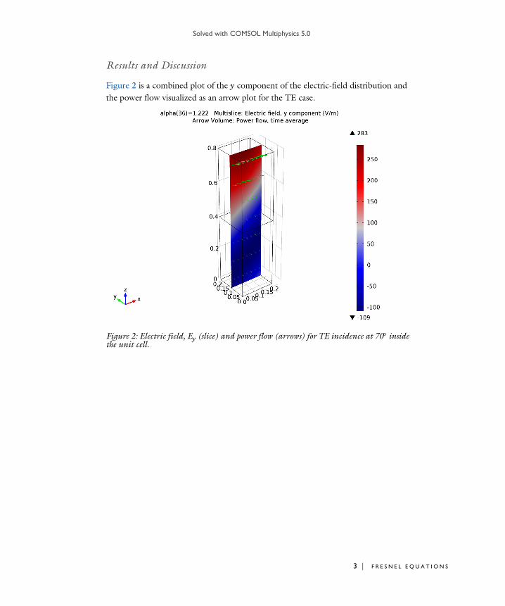
Figure 2 is a combined plot of the y component of the electric-field distribution and the power flow visualized as an arrow plot for the TE case.
Figure 2: Electric field, Ey (slice) and power flow (arrows) for TE incidence at 70 inside the unit cell.
3 | F R E S N E L E Q U A T I O N S

Solved with COMSOL Multiphysics 5.0
4 | F R E
For the TM case, Figure 3 visualizes the y component of the magnetic-field distribution instead, again in combination with the power flow.
Figure 3: Magnetic field, Hy (slice) and power flow (arrows) for TM incidence at 70 inside the unit cell.
Note that the sum of reflectance and transmittance in Figure 4 and Figure 5 equals 1, showing conservation of power. Figure 5 also shows that the reflectance around 56—the Brewster angle in the TM case—is close to zero.
S N E L E Q U A T I O N S

Solved with COMSOL Multiphysics 5.0
Figure 4: The reflectance and transmittance for TE incidence agree well with the analytic solutions.
Figure 5: The reflectance and transmittance for TM incidence agree well with the analytic solutions. The Brewster angle is also observed at the expected location.
5 | F R E S N E L E Q U A T I O N S

Solved with COMSOL Multiphysics 5.0
6 | F R E
References
1. C.A. Balanis, Advanced Engineering Electromagnetics, Wiley, 1989.
2. B.E.A. Saleh and M.C. Teich, Fundamentals of Photonics, Wiley, 1991.
Model Library path: Wave_Optics_Module/Verification_Models/fresnel_equations
Modeling Instructions
From the File menu, choose New.
N E W
1 In the New window, click Model Wizard.
M O D E L W I Z A R D
1 In the Model Wizard window, click 3D.
2 In the Select physics tree, select Optics>Wave Optics>Electromagnetic Waves,
Frequency Domain (ewfd).
3 Click Add.
4 Click Study.
5 In the Select study tree, select Preset Studies>Frequency Domain.
6 Click Done.
D E F I N I T I O N S
Define some parameters that are useful when setting up the mesh and the study.
Parameters1 On the Model toolbar, click Parameters.
2 In the Settings window for Parameters, locate the Parameters section.
S N E L E Q U A T I O N S

Solved with COMSOL Multiphysics 5.0
3 In the table, enter the following settings:
The angle of incidence is updated while running the parametric sweep. The refraction (transmitted) angle is defined by Snell's law with the updated angle of incidence. The Brewster angle exists only for TM incidence, p-polarization, and parallel polarization.
Variables 11 On the Model toolbar, click Variables and choose Local Variables.
2 In the Settings window for Variables, locate the Variables section.
Name Expression Value Description
n_air 1 1.0000 Refractive index, air
n_slab 1.5 1.5000 Refractive index, slab
lda0 1[m] 1.0000 m Wavelength
f0 c_const/lda0 2.9979E8 1/s Frequency
alpha 70[deg] 1.2217 rad Angle of incidence
beta asin(n_air*sin(alpha)/n_slab)
0.67701 rad Refraction angle
h_max lda0/6 0.16667 m Maximum element size, air
alpha_brewster
atan(n_slab/n_air) 0.98279 rad Brewster angle, TM only
r_s (n_air*cos(alpha)-n_slab*cos(beta))/(n_air*cos(alpha)+n_slab*cos(beta))
-0.54735 Reflection coefficient, TE
r_p (n_slab*cos(alpha)-n_air*cos(beta))/(n_air*cos(beta)+n_slab*cos(alpha))
-0.20613 Reflection coefficient, TM
t_s (2*n_air*cos(alpha))/(n_air*cos(alpha)+n_slab*cos(beta))
0.45265 Transmission coefficient, TE
t_p (2*n_air*cos(alpha))/(n_air*cos(beta)+n_slab*cos(alpha))
0.52925 Transmission coefficient, TM
7 | F R E S N E L E Q U A T I O N S
Solved with COMSOL Multiphysics 5.0
8 | F R E
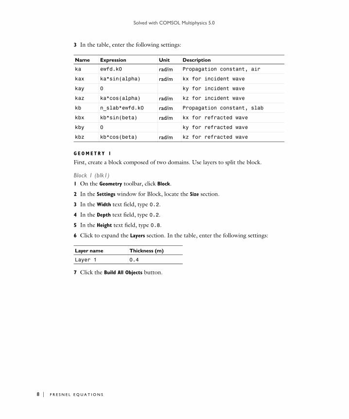
3 In the table, enter the following settings:
G E O M E T R Y 1
First, create a block composed of two domains. Use layers to split the block.
Block 1 (blk1)1 On the Geometry toolbar, click Block.
2 In the Settings window for Block, locate the Size section.
3 In the Width text field, type 0.2.
4 In the Depth text field, type 0.2.
5 In the Height text field, type 0.8.
6 Click to expand the Layers section. In the table, enter the following settings:
7 Click the Build All Objects button.
Name Expression Unit Description
ka ewfd.k0 rad/m Propagation constant, air
kax ka*sin(alpha) rad/m kx for incident wave
kay 0 ky for incident wave
kaz ka*cos(alpha) rad/m kz for incident wave
kb n_slab*ewfd.k0 rad/m Propagation constant, slab
kbx kb*sin(beta) rad/m kx for refracted wave
kby 0 ky for refracted wave
kbz kb*cos(beta) rad/m kz for refracted wave
Layer name Thickness (m)
Layer 1 0.4
S N E L E Q U A T I O N S
Solved with COMSOL Multiphysics 5.0
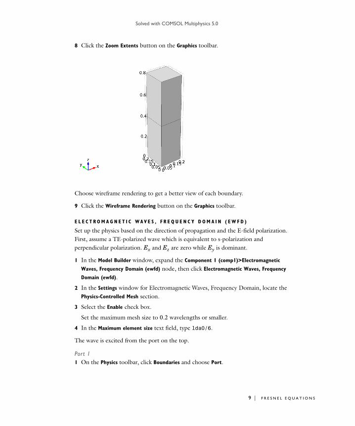
8 Click the Zoom Extents button on the Graphics toolbar.
Choose wireframe rendering to get a better view of each boundary.
9 Click the Wireframe Rendering button on the Graphics toolbar.
E L E C T R O M A G N E T I C WAV E S , F R E Q U E N C Y D O M A I N ( E W F D )
Set up the physics based on the direction of propagation and the E-field polarization. First, assume a TE-polarized wave which is equivalent to s-polarization and perpendicular polarization. Ex and Ez are zero while Ey is dominant.
1 In the Model Builder window, expand the Component 1 (comp1)>Electromagnetic
Waves, Frequency Domain (ewfd) node, then click Electromagnetic Waves, Frequency
Domain (ewfd).
2 In the Settings window for Electromagnetic Waves, Frequency Domain, locate the Physics-Controlled Mesh section.
3 Select the Enable check box.
Set the maximum mesh size to 0.2 wavelengths or smaller.
4 In the Maximum element size text field, type lda0/6.
The wave is excited from the port on the top.
Port 11 On the Physics toolbar, click Boundaries and choose Port.
9 | F R E S N E L E Q U A T I O N S

Solved with COMSOL Multiphysics 5.0
10 | F R E
2 Select Boundary 7 only.
3 In the Settings window for Port, locate the Port Properties section.
4 From the Wave excitation at this port list, choose On.
5 Locate the Port Mode Settings section. Specify the E0 vector as
6 In the text field, type abs(kaz).
Port 21 On the Physics toolbar, click Boundaries and choose Port.
2 Select Boundary 3 only.
3 In the Settings window for Port, locate the Port Mode Settings section.
4 Specify the E0 vector as
5 In the text field, type abs(kbz).
The bottom surface is an observation port. The S21-parameter from Port 1 and Port 2 provides the transmission characteristics.
The E-field polarization has Ey only and the boundaries are always either parallel or perpendicular to the E-field polarization. Apply periodic boundary conditions on the boundaries parallel to the E-field except those you already assigned to the ports.
Periodic Condition 11 On the Physics toolbar, click Boundaries and choose Periodic Condition.
2 Select Boundaries 1, 4, 10, and 11 only.
3 In the Settings window for Periodic Condition, locate the Periodicity Settings section.
4 From the Type of periodicity list, choose Floquet periodicity.
0 x
exp(-i*kax*x)[V/m] y
0 z
0 x
exp(-i*kbx*x)[V/m] y
0 z
S N E L E Q U A T I O N S

Solved with COMSOL Multiphysics 5.0
5 Specify the kF vector as
Apply a perfect electric conductor condition on the boundaries perpendicular to the E-field. This condition creates a virtually infinite modeling space.
Perfect Electric Conductor 21 On the Physics toolbar, click Boundaries and choose Perfect Electric Conductor.
kax x
0 y
0 z
11 | F R E S N E L E Q U A T I O N S

Solved with COMSOL Multiphysics 5.0
12 | F R E
2 Select Boundaries 2, 5, 8, and 9 only.
M A T E R I A L S
Now set up the material properties based on refractive index. The top half is filled with air.
Material 1 (mat1)1 In the Model Builder window, under Component 1 (comp1) right-click Materials and
choose Blank Material.
2 Select Domain 2 only.
3 In the Settings window for Material, locate the Material Contents section.
4 In the table, enter the following settings:
5 Right-click Component 1 (comp1)>Materials>Material 1 (mat1) and choose Rename.
6 In the Rename Material dialog box, type Air in the New label text field.
7 Click OK.
The bottom half is glass.
Property Name Value Unit Property group
Refractive index n n_air 1 Refractive index
S N E L E Q U A T I O N S

Solved with COMSOL Multiphysics 5.0
Material 2 (mat2)1 In the Model Builder window, right-click Materials and choose Blank Material.
2 Select Domain 1 only.
3 In the Settings window for Material, locate the Material Contents section.
4 In the table, enter the following settings:
5 Right-click Component 1 (comp1)>Materials>Material 2 (mat2) and choose Rename.
6 In the Rename Material dialog box, type Glass in the New label text field.
7 Click OK.
M E S H 1
1 In the Model Builder window, under Component 1 (comp1) right-click Mesh 1 and choose Build All.
S T U D Y 1
Step 1: Frequency Domain1 In the Model Builder window, under Study 1 click Step 1: Frequency Domain.
2 In the Settings window for Frequency Domain, locate the Study Settings section.
Property Name Value Unit Property group
Refractive index n n_slab 1 Refractive index
13 | F R E S N E L E Q U A T I O N S

Solved with COMSOL Multiphysics 5.0
14 | F R E
3 In the Frequencies text field, type f0.
Parametric Sweep1 On the Study toolbar, click Parametric Sweep.
2 In the Settings window for Parametric Sweep, locate the Study Settings section.
3 Click Add.
4 In the table, enter the following settings:
Use a direct solver instead of an iterative one for faster convergence.
Solution 11 On the Study toolbar, click Show Default Solver.
2 In the Model Builder window, expand the Study 1>Solver Configurations>Solution
1>Stationary Solver 1 node.
3 Right-click Direct and choose Enable.
4 Right-click Study 1>Solver Configurations>Solution 1>Stationary Solver 1>Direct and choose Compute.
R E S U L T S
Electric Field (ewfd)The default plot is the E-field norm for the last solution, which corresponds to tangential incidence. Replace the expression with Ey, add an arrow plot of the power flow (Poynting vector), and choose a more interesting angle of incidence for the plot.
1 In the Model Builder window, expand the Electric Field (ewfd) node, then click Multislice 1.
2 In the Settings window for Multislice, click Replace Expression in the upper-right corner of the Expression section. From the menu, choose Model>Component
1>Electromagnetic Waves, Frequency Domain>Electric>Electric field>ewfd.Ey - Electric
field, y component.
3 Locate the Multiplane Data section. Find the x-planes subsection. In the Planes text field, type 0.
4 Find the z-planes subsection. In the Planes text field, type 0.
5 Locate the Coloring and Style section. From the Color table list, choose Wave.
Parameter name Parameter value list Parameter unit
alpha range(0,2[deg],90[deg])
S N E L E Q U A T I O N S

Solved with COMSOL Multiphysics 5.0
6 In the Model Builder window, right-click Electric Field (ewfd) and choose Arrow
Volume.
7 In the Settings window for Arrow Volume, click Replace Expression in the upper-right corner of the Expression section. From the menu, choose Model>Component
1>Electromagnetic Waves, Frequency Domain>Energy and
power>ewfd.Poavx,...,ewfd.Poavz - Power flow, time average.
8 Locate the Arrow Positioning section. Find the y grid points subsection. In the Points text field, type 1.
9 Locate the Coloring and Style section. From the Color list, choose Green.
10 In the Model Builder window, click Electric Field (ewfd).
11 In the Settings window for 3D Plot Group, locate the Data section.
12 From the Parameter value (alpha (1)) list, choose 1.2217.
13 On the 3D plot group toolbar, click Plot.
14 Click the Zoom Extents button on the Graphics toolbar. The plot should look like that in Figure 2.
Add a 1D plot to see the reflection and transmission versus the angle of incidence.
1D Plot Group 21 On the Model toolbar, click Add Plot Group and choose 1D Plot Group.
2 In the Settings window for 1D Plot Group, locate the Plot Settings section.
3 Select the x-axis label check box.
4 In the associated text field, type Angle of Incidence.
5 Select the y-axis label check box.
6 In the associated text field, type Reflectance and Transmittance.
7 Click to expand the Legend section. From the Position list, choose Upper left.
8 On the 1D plot group toolbar, click Global.
9 In the Settings window for Global, locate the y-Axis Data section.
10 In the table, enter the following settings:
11 Click to expand the Coloring and style section. Locate the Coloring and Style section. Find the Line style subsection. From the Line list, choose None.
Expression Unit Description
abs(ewfd.S11)^2 1 Reflectance
abs(ewfd.S21)^2 1 Transmittance
15 | F R E S N E L E Q U A T I O N S

Solved with COMSOL Multiphysics 5.0
16 | F R E
12 Find the Line markers subsection. From the Marker list, choose Cycle.
13 Find the Line style subsection. From the Line list, choose None.
14 Find the Line markers subsection. From the Marker list, choose Cycle.
15 On the 1D plot group toolbar, click Global.
16 In the Settings window for Global, locate the y-Axis Data section.
17 In the table, enter the following settings:
18 On the 1D plot group toolbar, click Plot.
19 In the Model Builder window, right-click 1D Plot Group 2 and choose Rename.
20 In the Rename 1D Plot Group dialog box, type Reflection and Transmission in the New label text field.
21 Click OK. Compare the resulting plots with Figure 4.
The remaining instructions are for the case of TM-polarized wave, p-polarization, and parallel polarization. In this case, Ey is zero while Ex and Ez characterize the wave. In other words, Hy is dominant while Hx and Hz have no effect. Thus, the H-field is perpendicular to the plane of incidence and it is convenient to solve the model for the H-field.
E L E C T R O M A G N E T I C WA V E S , F R E Q U E N C Y D O M A I N ( E W F D )
Port 11 In the Settings window for Port, locate the Port Mode Settings section.
2 From the Input quantity list, choose Magnetic field.
3 Specify the H0 vector as
Port 21 In the Model Builder window, under Component 1 (comp1)>Electromagnetic Waves,
Frequency Domain (ewfd) click Port 2.
Expression Unit Description
abs(r_s)^2 Reflectance, analytic
n_slab*cos(beta)/(n_air*cos(alpha))*abs(t_s)^2
Transmittance, analytic
0 x
exp(-i*kax*x)[A/m] y
0 z
S N E L E Q U A T I O N S

Solved with COMSOL Multiphysics 5.0
2 In the Settings window for Port, locate the Port Mode Settings section.
3 From the Input quantity list, choose Magnetic field.
4 Specify the H0 vector as
Perfect Electric Conductor 2The model utilizes the H-field for the TM case and the remaining boundaries need to be perfect magnetic conductors.
1 In the Model Builder window, under Component 1 (comp1)>Electromagnetic Waves,
Frequency Domain (ewfd) right-click Perfect Electric Conductor 2 and choose Disable.
Perfect Magnetic Conductor 11 On the Physics toolbar, click Boundaries and choose Perfect Magnetic Conductor.
2 Select Boundaries 2, 5, 8, and 9 only.
To keep the solution and plots for the TE case, do as follows:
S T U D Y 1
Solution 11 In the Model Builder window, under Study 1>Solver Configurations right-click Solution
1 and choose Solution>Copy.
R E S U L T S
Electric Field (ewfd)1 Ctrl-click to select both Results>Electric Field (ewfd) and Results>Reflection and
Transmission, then right-click and choose Duplicate.
Electric Field (ewfd)1 In the Model Builder window, under Results click Electric Field (ewfd).
2 In the Settings window for 3D Plot Group, locate the Data section.
3 From the Data set list, choose Study 1/Solution 1 - Copy 1.
Reflection and Transmission1 In the Model Builder window, under Results click Reflection and Transmission.
2 In the Settings window for 1D Plot Group, locate the Data section.
0 x
exp(-i*kbx*x)[A/m] y
0 z
17 | F R E S N E L E Q U A T I O N S

Solved with COMSOL Multiphysics 5.0
18 | F R E
3 From the Data set list, choose Study 1/Solution 1 - Copy 1.
S T U D Y 1
On the Model toolbar, click Compute.
R E S U L T S
Electric Field (ewfd) 11 In the Model Builder window, expand the Results>Electric Field (ewfd) 1 node, then
click Multislice 1.
2 In the Settings window for Multislice, click Replace Expression in the upper-right corner of the Expression section. From the menu, choose Model>Component
1>Electromagnetic Waves, Frequency Domain>Magnetic>Magnetic field>ewfd.Hy -
Magnetic field, y component.
3 On the 3D plot group toolbar, click Plot. This reproduces Figure 3.
Reflection and Transmission 11 In the Model Builder window, expand the Results>Reflection and Transmission 1 node,
then click Global 2.
2 In the Settings window for Global, locate the y-Axis Data section.
3 In the table, enter the following settings:
4 On the 1D plot group toolbar, click Plot. The plot should look like Figure 5. The Brewster angle is observed around 56 degrees, which is close to the analytic value.
Expression Unit Description
abs(r_p)^2 Reflectance, analytic
n_slab*cos(beta)/(n_air*cos(alpha))*abs(t_p)^2
Transmittance, analytic
S N E L E Q U A T I O N S