solving dsge models with perturbation methods and a change ...jesusfv/change_variables.pdf · and a...

ARTICLE IN PRESS

Journal of Economic Dynamics & Control 30 (2006) 2509–2531

0165-1889/$ -

doi:10.1016/j

�CorrespoE-mail ad

www.elsevier.com/locate/jedc

Solving DSGE models with perturbation methodsand a change of variables

Jesus Fernandez-Villaverdea,�, Juan F. Rubio-Ramırezb

aDepartment of Economics, 160 McNeil Building, 3718 Locust Walk, University of Pennsylvania,

Philadelphia, PA 19104, USAbResearch Department, 1000 Peachtree St. NE, Federal Reserve Bank of Atlanta, Atlanta, GA 30309, USA

Received 24 November 2003; accepted 26 July 2005

Available online 1 December 2005

Abstract

This paper explores the application of the changes of variables technique to solve the

stochastic neoclassical growth model. We use the method of Judd [2003. Perturbation methods

with nonlinear changes of variables. Mimeo, Hoover Institution] to change variables in the

computed policy functions that characterize the behavior of the economy. We report how the

optimal change of variables reduces the average absolute Euler equation errors of the solution

of the model by a factor of three. We also demonstrate how changes of variables correct for

variations in the volatility of the economy even if we work with first-order policy functions and

how we can keep a linear representation of the laws of motion of the model if we use a nearly

optimal transformation. We discuss how to apply our results to estimate dynamic equilibrium

economies.

r 2005 Elsevier B.V. All rights reserved.

JEL classification: C63; C68; E37

Keywords: Dynamic equilibrium economies; Computational methods; Changes of variables; Linear and

nonlinear solution methods

see front matter r 2005 Elsevier B.V. All rights reserved.

.jedc.2005.07.009

nding author. Tel.: +1219 898 15 04; fax: +1215 573 20 57.

dress: [email protected] (J. Fernandez-Villaverde).

www.elsevier.com/locate/jedc

ARTICLE IN PRESS

J. Fernandez-Villaverde, J.F. Rubio-Ramırez / Journal of Economic Dynamics & Control 30 (2006) 2509–25312510

1. Introduction

This paper explores the application of the changes of variables technique to solvethe stochastic neoclassical growth model. In an important recent contribution, Judd(2003) has provided formulas to apply changes of variables to the solutions ofdynamic equilibrium economies obtained through the use of perturbationtechniques. Standard perturbation methods provide a Taylor expansion of thepolicy functions that characterize the equilibrium of the economy in terms of thestate variables of the model and a perturbation parameter. Judd’s derivations allowmoving from this Taylor expansion to any other series in terms of nonlineartransformations of the state variables without the need to recompute the wholesolution. This alternative approximation can be more accurate than the first becausethe change of variables induces nonlinearities that can help to track the true, butunknown, policy functions.

Judd’s results are important for several reasons. First, we often want to solveproblems with a large number of state variables. Solving these models is difficult andcostly. If we use perturbation methods, the number of derivatives required tocompute the parameters of the Taylor expansion of the solution quickly explodes aswe increase the order of the approximation (see Judd and Guu, 1997). Onealternative strategy is to obtain a low-order expansion (a quadratic or even just alinear one) of the solution and move to a more accurate representation using achange of variables. Computing this low-order expansion and the change ofvariables is relatively inexpensive. Consequently, if we are able to select an adequatetransformation, we can increase the accuracy of the solution enough to use ourcomputation for quantitative analysis despite the high dimensionality of the statespace.

Second, researchers frequently exploit approximated solutions to understand theanalytics of dynamic equilibrium models. See, for example, the classical treatment ofHall (1971) or the recent work of Woodford (2003). Because of tractabilityconsiderations, those analyses limit themselves to first-order expansions. Clearly theusefulness of this approach depends on the quality of the approximation. Linearsolutions, however, may perform poorly outside a small region around which welinearize. More importantly, as pointed out by Benhabib et al. (2001), linearsolutions may even lead to incorrect findings regarding the existence and uniquenessof equilibrium. An optimal change of variables can address both increase theaccuracy of the solution and avoid misleading local results while maintaininganalytic tractability.

Third, a change of variables can be useful to estimate dynamic equilibriumeconomies using a likelihood approach. In general, we do not know how to directlyevaluate the likelihood function of these economies. Consequently, we need to eitherlinearize the model and use the Kalman filter or to resort to simulation methods likethe particle filter that are expensive to implement (see Fernandez-Villaverde andRubio-Ramırez, 2004). A change of variables may deliver a representation of theeconomy suitable for efficient estimation while capturing some of the nonlinearitiesof the model.

ARTICLE IN PRESS

J. Fernandez-Villaverde, J.F. Rubio-Ramırez / Journal of Economic Dynamics & Control 30 (2006) 2509–2531 2511

Motivated by the arguments above, this paper applies Judd’s methodology to thestochastic neoclassical growth model with leisure, the workhorse of dynamicmacroeconomics. First, we derive a simple close-form relation between theparameters of the linear and the loglinear solution of the model. We extend thisapproach to a more general class of changes of variables: those that generate a policyfunction with a power function structure.

Second, we study the effects of that last particular class of changes of variable onthe size of the Euler equation errors, i.e., those errors that appear in the optimalityconditions of the agents because of the use of approximated solutions instead of theexact ones. We search for the optimal change of variable inside the class of powerfunctions and report results for a benchmark calibration of the model and foralternative parameterizations. In that way, we study the performance of theprocedure both for a nearly linear case (the benchmark calibration) and for morenonlinear cases (for example those with higher variance of the productivity shock).We find that, for the benchmark calibration, we reduce the average absolute Eulerequation errors by a factor of three. This reduction makes the new approximatedsolution of the model competitive to much more involved nonlinear methods, such asfinite elements or value function iteration, and to second-order perturbations.

Third, sensitivity analysis reveals how the change of variables corrects formovements in the exogenous variance of the economy through changes in theoptimal values of the parameters of the transformation. This is true even for a first-order approximation to the policy function. In comparison, a standard linear (orloglinear) solution can only provide a certainty equivalent approximation. Thisproperty is a key advantage of our approach.

Fourth, sensitivity analysis also suggests that a particular change of variables thatpreserves the linearity of the solution is roughly optimal. We propose the use of thisapproximation because of two reasons. First, because as explained before, suchlinearity allows researchers to use the well understood toolbox of linear systemswhile achieving a level of accuracy not possible with the standard linearization.Second, because it facilitates taking the model to the data. In addition to beinglinear, we show how this quasi-optimal approximated solution also implies that thedisturbances to the model are normally distributed. Consequently we can write theeconomy in a state-space form and use the Kalman filter to perform likelihood basedinference.

Finally, we extend some of our results to the change of variables in second-orderapproximations. We show how a change of variables noticeably increases theaccuracy of second-order approximations, even if those are already quite accuratewhen applied to the stochastic neoclassical growth model (see Aruoba et al., 2005,for details). Thus, our findings suggest that a second-order approximation with achange of variables is a highly attractive solution algorithm in terms of accuracy andsimplicity.

The rest of the paper is organized as follows. Section 2 presents the canonicalstochastic neoclassical growth model. Section 3 outlines how we solve for thestandard linear representation of the model policy functions in levels. Section 4discusses changes of variables in general terms. Section 5 derives the relation

ARTICLE IN PRESS


between the linear and loglinear solution of the model. Section 6 explores theoptimal change of variables within a flexible class of functions and reports asensitivity analysis exercise. Section 7 discusses the use of the change of variables forestimation. Section 8 extends some of our results to second-order approximations.Section 9 concludes.

2. The stochastic neoclassical growth model

As mentioned above, we want to explore how the approximated solutions of thestochastic neoclassical growth model with leisure respond to nonlinear changes ofvariables. Three reason lead us to use this model. First, its popularity (directly orwith small changes) to address a large number of questions (see Cooley, 1995) makesit a natural laboratory to explore the potential of Judd’s contribution. Second,because of this importance any analytical result regarding the (approximated)solution of the model is of interest in itself. Finally, since this model is nearly linearfor a benchmark calibration, its use provides a particularly difficult laboratory forthe change of variables approach: it bounds tightly the improvements we can obtain.We find important advantages of the technique even for this case. Consequently, theimprovements coming from the change of variables approach are likely to be higherfor more nonlinear economies.1

Since the model is well known (see Cooley and Prescott, 1995), we provide only theminimum exposition required to fix notation. There is a representative agent in theeconomy, whose preferences over stochastic sequences of consumption ct and leisure1� lt are representable by the utility function:

E0

X1t¼0

btUðct; ltÞ,

where b 2 ð0; 1Þ is the discount factor, E0 is the conditional expectation operator andUð�; �Þ satisfies the usual technical conditions.

There is one good in the economy, produced according to the aggregateproduction function yt ¼ eztka

t l1�at where kt is the aggregate capital stock, lt is theaggregate labor input, and zt is a stochastic process representing randomtechnological progress. The technology follows a first-order process zt ¼ rzt�1 þ �twith jrjo1 and �t�Nð0;s2Þ. Capital evolves according to the law of motion ktþ1 ¼

ð1� dÞkt þ it where d is the depreciation rate and the economy must satisfy theresource constraint yt ¼ ct þ it.

Since both welfare theorems hold in this economy, we can solve directly for thesocial planner’s problem. We maximize the utility of the household subject to theproduction function, the evolution of the stochastic process, the law of motion for

1The special case of the neoclassical growth model with log utility function and total depreciation is not

very informative regarding the usefulness of a change of variables: we already know that the exact solution

of that case is loglinear. We want to evaluate the performance of those changes of variables in the general

situation where we do not have an analytical solution.

ARTICLE IN PRESS


capital, the resource constraint and some initial conditions for capital and thestochastic process.

The solution to this problem is fully characterized by the equilibrium conditions:

UcðtÞ ¼ bEtfUcðtþ 1Þð1þ aeztþ1ka�1tþ1 l1�atþ1 � dÞg,

UlðtÞ ¼ �UcðtÞð1� aÞeztkat l�at ,

ct þ ktþ1 ¼ ezt kat l1�at þ ð1� dÞkt,

zt ¼ rzt�1 þ et

given some initial capital and some initial value for the stochastic process fortechnology. The first equation is the standard Euler equation that relates current andfuture marginal utilities from consumption, the second one is the static first-ordercondition between labor and consumption, and the last two equations are theresource constraint of the economy and the law of motion of technology.

We solve for the equilibrium of this economy by finding two policy functions fornext period’s capital k0ð�; �; �Þ, and labor lð�; �; �Þ, which deliver the optimal choice ofthese controls as functions of the two state variables, capital and technology level,and the standard deviation of the innovation to the productivity level s. Using thebudget constraint, cð�; �; �Þ is a function of kð�; �; �Þ and lð�; �; �Þ. Note that we includethe perturbation parameter as one explicit variable in the policy functions. Thatnotation is convenient for the next section.

3. Solving the model using a perturbation approach

The system of equations listed above does not have a known analytical solutionand we need to use a numerical method to solve it. In a series of seminal papers, Juddand coauthors (see Judd and Guu, 1992, 1997 and the textbook exposition inJudd, 1998, among others) have proposed to build a Taylor series expansion of thepolicy functions k0ð�; �; �Þ, and lð�; �; �Þ around the deterministic steady state wherez ¼ 0 and s ¼ 0.

If k0 is equal to the value of the capital stock in the deterministic steady state andthe policy function for labor is smooth, we can use a Taylor series to approximatethis policy function around ðk0; 0; 0Þ with the form

lpðk; z; sÞ ’Xi;j;m

1

ði þ j þmÞ!

qiþjþmlpðk; z; sÞ

qkiqzjqsm

��k0;0;0

ðk � k0Þizjsm,

where the subscript p stands for perturbation approximation. The policy function fornext period capital will have an analogous representation.

The key idea of the perturbation methods is to set the parameter s equal to zero(since in this case the model can be solved analytically) and to exploit implicit-

function theorems to pin down the unknown coefficientsqiþjþmlpðk;z;sÞ

qkiqzjqsm jk0;0;0 in a

recursive fashion.

ARTICLE IN PRESS


To do so, the first step is to linearize the equilibrium conditions of the modelaround the deterministic steady state, i.e. when s ¼ 0. Then, we substitute capitaland labor by the values given by the first-order expansion of the policy function andwe solve for the unknown coefficients. The next step is to find the second-orderexpansion of the equilibrium conditions, again around the deterministic steady state,plug in the quadratic approximation of the policy function (evaluated with the first-order coefficients found before) and solve for the unknown second-order coefficients.We can iterate on this procedure as many times as desired to get an approximation ofarbitrary order. For a more detailed explanation of these steps we refer the reader toJudd and Guu (1992).

Since perturbations only deliver an asymptotically locally correct expression forthe policy functions, the accuracy achieved by the method may be poor either awayfrom the deterministic steady state or when the order of the expansion is low.

Several routes have been proposed to correct for these problems. One, by Collardand Juillard (2001), uses bias correction to find the approximation of the solutionaround a more suitable point that the deterministic steady state. The second one,suggested by Judd (2003), changes the variables in terms of which we express thecomputed solution of the model. We review Judd’s proposal in next section.

4. The change of variables

The first-order perturbation solution to the stochastic neoclassical growth modelcan be written as f ðxÞ ’ f ðaÞ þ ðx� aÞf 0ðaÞ where x ¼ ðk; zÞ are the variables of theexpansion, a ¼ ðk0; 0Þ is the deterministic steady-state value of those variables, andf ðxÞ ¼ ðk0pðk; zÞ; lpðk; zÞÞ is the unknown policy function of the model. Since the first-order perturbation solution does not depend on s, we drop it in this section to saveon notation. We could easily consider higher order perturbation solutions, but weconcentrate in the first-order approximations because of expositional reasons.

Let us now transform both the domain and the range of f ðxÞ. Thus, to expresssome nonlinear function of f ðxÞ, hðf ðxÞÞ : R2

! R2 as a polynomial in sometransformation of x, Y ðxÞ : R2

! R2, we can use the Taylor series of gðyÞ ¼

hðf ðX ðyÞÞÞ around b ¼ Y ðaÞ, where X ðyÞ is the inverse of Y ðxÞ.Using the chain rule, Judd (2003) shows that

gðyÞ ¼ hðf ðX ðyÞÞÞ ¼ gðbÞ þ GðbÞðY ðxÞ � bÞ, (1)

where GðbÞ is a 2� 2 matrix, whose i; j entry is

Gij ¼X

m

qhi

qf m

Xn

qf m

qX n

qX n

qyj.

From this expression we see that if we have computed the values of partialderivatives of f, it is straightforward to find the value of G.

In the next two sections we obtain particular values for this general transforma-tion, one for moving between a solution in levels and in logs and a second for a moregeneral class of power functions.

ARTICLE IN PRESS


5. A particular case: the loglinearization

Since the exact solution of the stochastic neoclassical growth model in the case oflog utility and d ¼ 1 is loglinear, many practitioners have favored the loglineariza-tion of the equilibrium conditions of the model over linearization in levels.2 Thispractice generates the natural question of finding the relation between thecoefficients on both representations. We use (1) to get a simple closed-form answerto this question.

A first-order perturbation produces an approximated policy function in levels ofthe form3

ðk0 � k0Þ ¼ a1ðk � k0Þ þ b1z,

ðl � l0Þ ¼ c1ðk � k0Þ þ d1z,

where k and z are the current states of the economy, l0 is steady-state value for labor,and where, for convenience, we have dropped the subscript p where no ambiguityexists. As mentioned before, all the coefficients on s are zero in the first-orderperturbation.

Analogously a loglinear approximation of the policy function will take the form

log k0 � log k0 ¼ a2ðlog k � log k0Þ þ b2z,

log l � log l0 ¼ c2ðlog k � log k0Þ þ d2z,

or in equivalent notation:bk0 ¼ a2bk þ b2z,bl ¼ c2bk þ d2z,

where bx ¼ log x� log x0 is the percentage deviation of the variable x with respect toits steady state.

How do we go from one approximation to the second one? First, we follow Judd’s(2003) notation and write the linear system in levels as

k0pðk; z;sÞ ¼ f 1ðk; z; sÞ ¼ f 1

ðk0; 0; 0Þ þ f 11ðk0; 0; 0Þðk � k0Þ þ f 1

2ðk0; 0; 0Þz,

lpðk; z;sÞ ¼ f 2ðk; z;sÞ ¼ f 2

ðk0; 0; 0Þ þ f 21ðk0; 0; 0Þðk � k0Þ þ f 2

2ðk0; 0; 0Þz,

where

2The wisdom of this practice is disputab

(2005) for two papers that find that linear3See Uhlig (1999) for details. Remember

quadratic approximation of the utility

decomposition (Blanchard and Kahn, 198

2000) or the QZ decomposition (Sims, 200

same policy functions since the linear spac

le. See for example, Dotsey and Mao (1992

ization performs better than loglinearizatio

that this solution is the same as the one g

function (Kydland and Prescott, 198

0; King et al., 2002), generalized Schur de

2b) among others. Subject to applicability,

e approximating a nonlinear space is uniq

f 1ðk0; 0; 0Þ ¼ k0
f 1
1ðk0; 0; 0Þ ¼ a1
f 12ðk0; 0; 0Þ ¼ b1
f 2ðk0; 0; 0Þ ¼ l0
f 2
1ðk0; 0; 0Þ ¼ c1
f 22ðk0; 0; 0Þ ¼ d1
) and Aruoba et al.

n.

enerated by a linear

2), the eigenvalue

composition (Klein,

all methods find the

ue.

ARTICLE IN PRESS


Second, we propose the changes of variables:

4An alternative heuristic argument that

ðk0 � k0Þ ¼ a1ðk � k0Þ þ b1z,

ðl � l0Þ ¼ c1ðk � k0Þ þ d1z.

and divide on both sides by the steady-sta

k0 � k0

k0¼ a1

k � k0

k0þ

1

k0b1z,

l � l0

l0¼ c1

k � k0

l0þ

1

l0d1z.

Sincex0�x0

x0’ log x� log x0, we get the sam

more general and does not depend on an

delivers the same result is as follows. Take the

te value of the control variable:

e relation that the one presented in the paper. O

additional approximation.

h1¼ log f 1
Y 1ðxÞ ¼ log x1 X 1 ¼ exp y1
h2¼ log f 2
Y 2 ¼ x2 X 2 ¼ y2
Judd’s (2003) formulas for this particular example imply

log k0ðlog k; zÞ

log lðlog k; zÞ

!¼ gðlog k; zÞ ¼

log f 1ðk0; 0; 0Þ

log f 2ðk0; 0; 0Þ

!

þ

1

k0f 11ðk0; 0; 0Þk0

1

k0f 12ðk0; 0; 0Þ

1

l0f 21ðk0; 0; 0Þk0

1

l0f 22ðk0; 0; 0Þ

0BBB@1CCCA log k � log k0

z

!,

and thus

log k0 � log k0 ¼ f 11ðk0; 0; 0Þðlog k � log k0Þ þ

1

k0f 12ðk0; 0; 0Þz,

log l � log l0 ¼k0

l0f 21ðk0; 0; 0Þðlog k � log k0Þ þ

1

l0f 22ðk0; 0; 0Þz.

By equating coefficients we obtain a simple closed-form relation between theparameters of both representations:4

system

ur argum
ent
a2 ¼ a1
b2 ¼1
k0b1

c2 ¼k0l0

c1
d2 ¼1l0
d1

Note that we have not used any assumption on the utility or production functionsexcept that they satisfy the general technical conditions of the neoclassical growth

is

ARTICLE IN PRESS


model. Also, moving from one coefficient set to the other one is an operation thatonly involves k0 and l0, values that we need to find anyway to compute the linearizedversion in levels. Therefore, once you have the linear solution, obtaining the loglinearone is immediate.

6. The optimal change of variables

In the last section, we showed how to find a loglinear approximation to the solutionof the neoclassical growth model directly from its linear representation. Now, wegeneralize our result to encompass the relationship between any power functionapproximation and the linear coefficients of the policy function. Also, we search forthe optimal change of variable inside this class of power functions and we report howthe Euler equation errors improve with respect to the linear representation.

6.1. A power function transformation

Before, we argued that some practitioners have defended the use of loglineariza-tions to capture some of the nonlinearities in the data. This practice can be pushedone step ahead. We can generalize the log function into a general class of powerfunction of the form

k0pðk; z; g; z; mÞg� k

g0 ¼ a3ðk

z� kz

0Þ þ b3z,

lpðk; z; g; z;mÞm� l

m0 ¼ c3ðk

z� kz

0Þ þ d3z.

This class of functions is attractive because it provides a lot of flexibility in shapeswith only three free parameters, while including the log transformation as the limitcase when the coefficients g, z, and m tend to zero. A similar power function with onlytwo parameters is proposed by Judd (2003) in a growth model without leisure andstochastic perturbations. His finding of notable improvements in the accuracy of thesolution when he optimally selects the value of these parameters is suggestive of theadvantages of using this parametric family.

The changes of variables for this family of functions are given by

h1¼ ðf 1

Þg
Y 1 ¼ ðx1Þ
z
X 1 ¼ ðy
1Þ1z

h2¼ ðf 1

Þm
Y 2 ¼ x2 X 2 ¼ y2
Following the same reasoning than in the previous section, we derive a form forthe system in term of the original coefficients:


g0 ¼

gz

kg�z0 a1ðk

z� kz

0Þ þ gkg�10 b1z,


m0 ¼

mz

lm�10 k1�z

0 c1ðkz� kz

0Þ þ mlm�10 d1z.

ARTICLE IN PRESS


Therefore, the relation of between the new and the old coefficients is again simple tocompute:

a3 ¼gz k

g�z0 a1
b3 ¼ gk
g�10 b1

c3 ¼mz l

m�10 k1�z

0 c1
d3 ¼ mlm�10 d1
6.2. Searching for the optimal transformation

One difference between the transformation from linear into a loglinear solutionand the current transformation into a power law is that we have three freeparameters g, z, and m. How do we select optimal values for those?

A reasonable criterion is to select them in order to improve the accuracy of thesolution of the model. This desideratum raises a question. How do we measure thisaccuracy, conditional on the fact that we do not know the true solution of the model?

Judd and Guu (1992) solves this problem evaluating the normalized Eulerequation errors (see also Santos, 2000; Den Haan and Marcet, 1994). Note that inour model intertemporal optimality implies that

UcðtÞ ¼ bEtfUcðtþ 1Þð1þ aeztþ1ka�1tþ1 l1�atþ1 � dÞg. (2)

Since the solutions are not exact, condition (2) will not hold exactly when evaluatedusing the computed decision rules. Instead, for any choice of g, z, and m and itsassociated policy rules k0pð�; �; g; z;mÞ and lpð�; �; g; z;mÞ, we can define the normalizedabsolute value Euler equation errors as

EEðk; z;XÞ ¼ 1�ðU�1c ðEtUcðtþ 1ÞbR0ðk; z;XÞ; lpðk; z;XÞÞÞ

cpðk; z;XÞ

�� , (3)

where X ¼ ðg; z;mÞ, R0ðk; z;XÞ ¼ ð1þ aeztþ1k0ðk; z;XÞa�1l0ðk; z;XÞ1�a � dÞ is the grossreturn on capital next period, and where we have used the static optimality conditionto substitute labor by its optimal choice.

This expression evaluates the (unit free) error in the Euler equation measured as afraction of cpð�; �;XÞ as a function of the current states k, and z, and the change ofvariables defined by g, z, and m. Judd and Guu (1997) interpret this function as themistake, in dollars, incurred by each dollar spent. For example, EEðk; z;XÞ ¼ 0:01means that the consumer makes a 1 dollar mistake for each 100 dollar spent.

Our criterion is to select values of X that minimize the Euler error function. But herewe face another problem. This function depends not only on the parameters X, butalso on the values of the state variables. How do we eliminate that dependency? Do weminimize the Euler equation error at one particular point of the state space like thedeterministic steady state? Do we minimize instead some weighted mean of it?

A first choice could be the criterion minXR

EEðk; z;XÞdF where F is thestationary distribution of k and z. This choice is intuitive. We would weight eachEuler equation error by the percentage of the time that the economy spends in that

ARTICLE IN PRESS


particular point: we would want to nail down the Euler equation errors for thoseparts of the stationary distribution where most of the action would happen, while wewould care less about accuracy in those points not frequently visited. The difficultyof the criterion is that we do not know that true stationary distribution (at least forcapital) before we find the policy functions of the model.

To avoid this difficulty, we could solve a fixed-point problem where we get someapproximation of the model, compute a stationary distribution, resolve theminimization problem, find the new stationary distribution, and continue untilconvergence. This approach faces two problems. First, it would be expensive incomputing time. Second, there is no known theory result that guarantees theconvergence of such iteration to the right set of values for the parameters of thetransformation.

Given the difficulties of the previous approach, we follow a simpler strategy.Inspired by collocation schemes in projection methods, we minimize the Eulerequation errors over a grid of points of k and z:

minX

SEEðXÞ ¼ minX

Xk;z

EEðk; z;XÞ. (4)

Setting this grid around the deterministic steady state (big enough to berepresentative of the stationary distribution of the economy but not too wide toavoid minimization over regions infrequently visited) may achieve our desire goal ofimproving the accuracy of the solution.5

Inspection of (4) reveals that this problem depends on the values of the structuralparameters of the model, i.e. those describing preferences and technology.Consequently, we need to take a stand on those before we can report any result.We will calibrate of the model to match basic observations of the US economyfollowing the common strategy in macroeconomics and, later, perform sensitivityanalysis. Hence, we evaluate how much accuracy we win in a ‘real life’ situation byapplying our change of variables and how confident we are in our results.

First we select as our utility function the CRRA form

ðcyt ð1� ltÞ1�yÞ1�t

1� t,

where t determines the elasticity of intertemporal substitution and y controls laborsupply. Then we pick the benchmark calibration values as follows. The discountfactor b ¼ 0:99 matches an annual interest rate of 4 percent. The parameter thatgoverns risk aversion t ¼ 2 is a common choice in the literature. y ¼ 0:36 matches

5When judging this scheme we need to remember that we do not look for the absolute best change of

variables (although certainly finding it would be nice) but for an improvement in the accuracy of the

solution that can be easily found. This point can be important in models with dozens of state variables,

where a multivariate maximization may be very costly. We can use a simulation procedure like a Markov

chain Monte Carlo method to find an improvement ‘sufficiently good’. Those approaches are easy to code

and get close to a global maximum (although not exactly at it) fairly quickly. In this paper, however, we

can solve the problem using a Newton algorithm implemented in a Mathematica notebook that is available

online at the following URL http://www.econ.upenn.edu/�jesusfv

http://www.econ.upenn.edu/jesusfv

http://www.econ.upenn.edu/jesusfv

ARTICLE IN PRESS


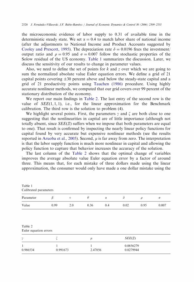
the microeconomic evidence of labor supply to 0.31 of available time in thedeterministic steady state. We set a ¼ 0:4 to match labor share of national income(after the adjustments to National Income and Product Accounts suggested byCooley and Prescott, 1995). The depreciation rate d ¼ 0:0196 fixes the investment/output ratio and r ¼ 0:95 and s ¼ 0:007 follow the stochastic properties of theSolow residual of the US economy. Table 1 summarizes the discussion. Later, wediscuss the sensitivity of our results to change in parameter values.

Also, we need to define the set of points for k and z over which we are going tosum the normalized absolute value Euler equation errors. We define a grid of 21capital points covering �30 percent above and below the steady-state capital and agrid of 21 productivity points using Tauchen (1986) procedure. Using highlyaccurate nonlinear methods, we computed that our grid covers over 99 percent of thestationary distribution of the economy.

We report our main findings in Table 2. The last entry of the second row is thevalue of SEEð1; 1; 1Þ, i.e., for the linear approximation for the Benchmarkcalibration. The third row is the solution to problem (4).

We highlight several points. First, the parameters g and z are both close to onesuggesting that the nonlinearities in capital are of little importance (although nottotally absent, since SEEðXÞ suffers when we impose that both parameters are equalto one). That result is confirmed by inspecting the nearly linear policy functions forcapital found by very accurate but expensive nonlinear methods (see the resultsreported in Aruoba et al., 2005). Second, m is far away from zero. The interpretationis that the labor supply function is much more nonlinear in capital and allowing thepolicy function to capture that behavior increases the accuracy of the solution.

The last column of the Table 2 shows that the optimal change of variablesimproves the average absolute value Euler equation error by a factor of aroundthree. This means that, for each mistake of three dollars made using the linearapproximation, the consumer would only have made a one dollar mistake using the

Table 1

Calibrated parameters

Parameter b t y a d r s

Value 0.99 2.0 0.36 0.4 0.02 0.95 0.007

Table 2

Euler equation errors

g z m SEEðXÞ

1 1 1 0.0856279

0.986534 0.991673 2.47856 0.0279944

ARTICLE IN PRESS


optimal change of variable, a sizeable (but not dramatic) improvement in accuracy.This same result is shown in Fig. 1, where we plot the decimal log of the absoluteEuler equation errors at z ¼ 0 for the ordinary linear solution and the optimalchange of variable. The use of decimal logs eases the reading of the graph. A value of�3 in the vertical axis represents an error of 1 dollar out of each 1000 dollars, a valueof �4 an error of 1 dollar out of each 10,000 dollars and so on. In Fig. 1, we observethat when only one dimension is considered, the optimal change of variable canimprove Euler equation errors from around 1 dollar every 10,000 dollars to 1 dollarevery 1,000,000 dollars (an even more in some points).

We explore how the optimal change of variable compares with other moreconventional nonlinear methods in terms of accuracy. In Fig. 2, we compare theEuler equation errors generated by the optimal change of variables with the Eulererrors implied by different linear and nonlinear solution methods (see Aruoba et al.,2005, for details about the other methods). The graph shows how the optimal changeof variable solution pushes a first-order approximation to the accuracy leveldelivered by the finite elements method for most of the interval. If we consider thecomputational and coding costs of implementing the finite elements method, thisresult provides strong evidence in favor of using a combination of linear solution andoptimal change of variable as a solution method for macroeconomic models. Also,the new approximation is roughly comparable in terms of accuracy with a second-order approximation of the policy function defended by Sims (2002a) and Schmitt-Grohe and Uribe (2004).

We finish by pointing out how the change of variables might have the additionaladvantage of suffering less often from the problem of explosive behavior ofsimulations present in the second and higher order perturbations. This explosivebehavior appears because of the presence of higher order terms in the perturbationsolution. Sometimes, the productivity shocks are so big that the high powers of the

18 20 22 24 26 28 30-8

-7.5

-7

-6.5

-6

-5.5

-5

-4.5

-4

-3.5

Capital

Log1

0 |E

uler

Equ

atio

n E

rror

|

Linear

Change of Variables

Fig. 1. Euler equation errors at z ¼ 0; t ¼ 2=s ¼ 0:007.

ARTICLE IN PRESS

18 20 22 24 26 28 30

-9

-8

-7

-6

-5

-4

-3

Capital

Log1

0 |E

uler

Equ

atio

n E

rror

|Linear

5th Order Perturbation

FEM

2nd Order Perturbation Change of Variables

Loglinear



solution send the path of capital outside the stable manifold. For example, Aruoba etal. (2005) find that, for a model like the one studied in this paper, up to 4 percent ofthe simulations led to explosive paths when they use a fifth-order approximation.There are two solutions to this problem. First, those explosive simulation can beeliminated from the computation. However, there is a certain degree of arbitrarinessin the definition of when a path becomes explosive. Second, Kim et al. (2003)propose an algorithm that always produces stationary second-order accuratedynamics whenever the first-order dynamics are stable.

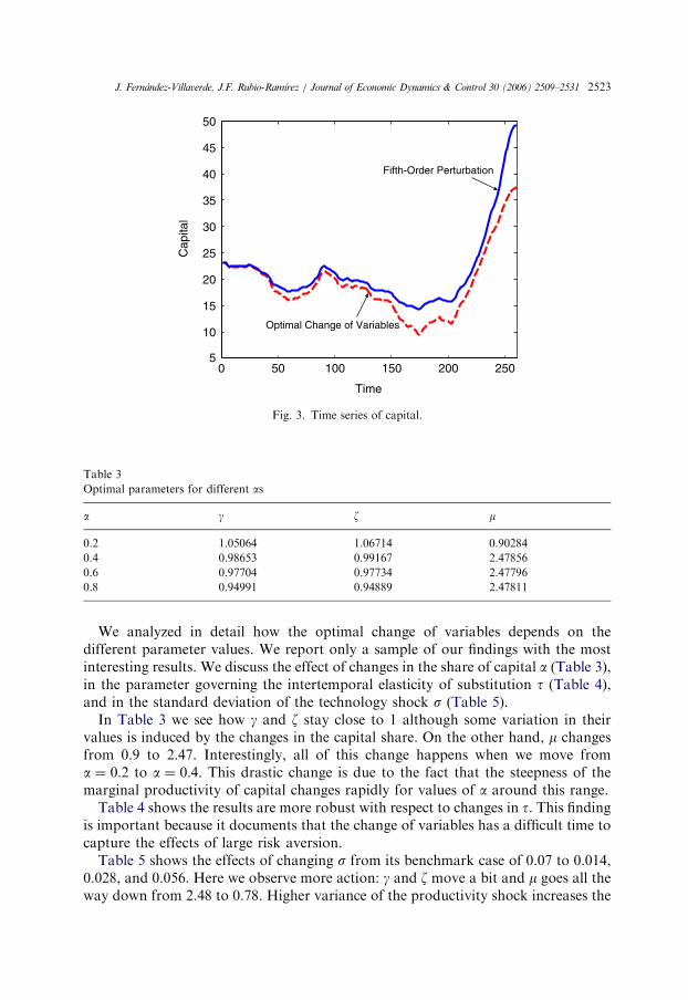
The change of variables suffers less from the problem of explosive paths because itraises the state variables at lower powers. In our application, the powers in the policyfunction for capital (the one exposed to explosive behavior) vary from 0.97 to 1.24.These lower powers stop most explosive paths. An example can be seen in Fig. 3. Wedraw two simulated time series of capital for our model with s ¼ 0:56 (the highervariance of productivity shocks needed to show more clearly the presence ofexplosive paths). The first line plots the series of capital induced by a fifth-orderperturbation. The second line plots the series of capital for the optimal change ofvariables. From this figure we can see how for the first 150 periods, both series areclose. However, around period 175 they separate and, after a few periods, thesimulation from the fifth-order explodes while the simulation from the optimalchange of variables, despite also showing an increase in the amount of capital, stayswithin the stable manifold.

6.3. Sensitivity analysis

How does the solution to (4) depend on the chosen calibration? Are the optimalparameters values in X robust to changes in the values of the structural parameters ofthe economy?

ARTICLE IN PRESS

0 50 100 150 200 2505

10

15

20

25

30

35

40

45

50

Time

Cap

ital

Fifth-Order Perturbation

Optimal Change of Variables

Fig. 3. Time series of capital.

Table 3

Optimal parameters for different as

a g z m

0.2 1.05064 1.06714 0.90284

0.4 0.98653 0.99167 2.47856

0.6 0.97704 0.97734 2.47796

0.8 0.94991 0.94889 2.47811


We analyzed in detail how the optimal change of variables depends on thedifferent parameter values. We report only a sample of our findings with the mostinteresting results. We discuss the effect of changes in the share of capital a (Table 3),in the parameter governing the intertemporal elasticity of substitution t (Table 4),and in the standard deviation of the technology shock s (Table 5).

In Table 3 we see how g and z stay close to 1 although some variation in theirvalues is induced by the changes in the capital share. On the other hand, m changesfrom 0.9 to 2.47. Interestingly, all of this change happens when we move froma ¼ 0:2 to a ¼ 0:4. This drastic change is due to the fact that the steepness of themarginal productivity of capital changes rapidly for values of a around this range.

Table 4 shows the results are more robust with respect to changes in t. This findingis important because it documents that the change of variables has a difficult time tocapture the effects of large risk aversion.

Table 5 shows the effects of changing s from its benchmark case of 0.07 to 0.014,0.028, and 0.056. Here we observe more action: g and z move a bit and m goes all theway down from 2.48 to 0.78. Higher variance of the productivity shock increases the

ARTICLE IN PRESS

Table 4

Optimal parameters for different ts

t g z m

4 1.02752 1.03275 2.47922

10 1.04207 1.04671 2.47830

50 1.01138 1.01638 2.47820

Table 5

Optimal parameters for different ss

s g z m

0.014 0.98140 0.98766 2.47753

0.028 1.04804 1.05265 1.73209

0.056 1.23753 1.22394 0.77869


precautionary motive for consumers and induces stronger nonlinearities in thecomputed policy functions of the model.

The variation in optimal parameter values is a significant result. It shows how thechange of variables allows for a correction based on the level of uncertainty existingin the economy. This correction cannot be achieved by linearization approach sincethat strategy produces a certainty equivalent approximation. The ability to adapt todifferent volatilities while keeping a first-order structure in the solution is a keyadvantage of the change of variables procedure.

We conclude from our sensitivity analysis that the choices of optimal parametervalues of g, z, and m are stable across very different parameterizations and that theonly relevant change is for the value of m when we vary capital share or the varianceof the technology shock.

6.4. A linear representation of the solution

Our previous findings motivate the following observation. Since g and z areroughly equal across different parameterizations, we can confine ourselves to the twoparameter transformation:

k0g� k

g0 ¼ a3ðk

g� k

g0Þ þ b3z,

lm � lm0 ¼ c3ðk

g� k

g0Þ þ d3z,

while keeping nearly all the same level of accuracy obtained by the more generalcase.

To illustrate our point we plot the Euler Equation error for this restricted optimalcase in Fig. 4 with g ¼ 1:11498 and m ¼ 0:948448. Comparing with the optimalchange we can appreciate how we keep nearly all the increment in accuracy. Moreformally the SEEðXÞ moves now to 0.0420616.

ARTICLE IN PRESS

18 20 22 24 26 28 30-8

-7.5

-7

-6.5

-6

-5.5

-5

-4.5

-4

-3.5

Capital

Log1

0 |E

uler

Equ

atio

n E

rror

|

Linear

OptimalChange

Restricted Optimal Change



The proposed two parameter transformation is very convenient because if wedefine bk ¼ kg

� kg0 and bl ¼ lm � l

m0 we can rewrite the equations asbk0 ¼ a3

bk þ b3z,bl ¼ c3bk þ d3z

producing a linear system of difference equations.This implies that we can study the neoclassical growth model (or a similar dynamic

equilibrium economy) in the following way. First, we find the equilibrium conditionsof the economy. Second, we linearize them (or loglinearize if it is easier) and solve theresulting problem using standard methods. Third, we transform the variables (leavingthe parameters of the transformation undetermined until the final numerical analysis)and study the qualitative properties of the new system using standard techniques. Ifthe transformation captures some part of the nonlinearities of the problem we may beable to avoid the problems singled out by Benhabib et al. (2001). Fourth, if we want tostudy the quantitative behavior of the economy we pick values for the parametersaccording to (4) and simulate the economy using the transformed system.

7. Changes of variables for estimation

Often, dynamic equilibrium models can be written in a state-space representation,with a transition equation that determines the law of motion for the states and ameasurement equation that relates states and observables. It is well known thatmodels with this representation are easily estimated using the Kalman Filter (seeHarvey, 1989).

ARTICLE IN PRESS


Consequently, a common practice to take the stochastic neoclassical growthmodel to the data has been to linearize the equilibrium conditions in levels or in logsaround the steady state to get a transition and a measurement equation, use theKalman recursion to evaluate the implied likelihood, and then, either to maximize it(in a classical perspective) or to draw from the posterior (in a Bayesian approach).

In this subsection we propose a variation of this strategy. Since in ourcomputations we find that g and z are roughly equal, we propose to usebk0 ¼ a3

bk þ b3z (5)

in the transition equation and (possibly)bl ¼ c3bk þ d3z (6)

in the measurement equation, where bk ¼ kg� k

g0 and

bl ¼ lm � lm0, instead of the usual

linear or loglinear relations. Since both equations are still linear in the transformedvariables, the conditional distributions of the variables is normal and we can use theKalman Filter to evaluate the likelihood. The only difference now will be that, inaddition to depend on the structural parameters of the model, the likelihood will alsobe a function of the parameters g and m.

This approach allows us to keep a linear representation suitable for efficientestimation while capturing an important part of the nonlinearities of the model andavoiding the use of expensive simulation methods like a particle filter.

To illustrate the potentiality of our proposal, we proceed as follows. First, wegenerate 200 observation of ‘artificial’ data for hours worked, lT ¼ fltg

200t¼1, from the

stochastic neoclassical growth model that we presented above. We solved the modelusing the finite elements method as described in Aruoba et al. (2005) to generate anartificial sample with nonlinearities. Second, we compute the likelihood functionimplied by the approximated solution (5) and (6), where g and z are chosen tominimize the problem (4). For comparison purposes, we compute the likelihoodimplied by the loglinear solution. We evaluate both likelihood functions at the sameparameter values that we use to generate the ‘artificial’ data for hours worked.

A simple procedure to compare both solutions is to implement a likelihood ratiotest. This test will tells which of the two models, the one represented by (5) and (6) orthe usual loglinear model, fits the data better.

We compute the likelihood ratio test for two different points in the parameterspace. First, we use the parameter values described in our benchmark calibration.Second, we also consider a more extreme case where t ¼ 50 and s ¼ 0:035, while wemaintain the value of the rest of the parameters to the values reported in Table 1. Werecognize that the extreme case (high risk aversion/high variance) is not realistic, butit allows us to easily consider a very nonlinear case.6

The likelihood ratio is defined by

bl ¼ LRðlTjY; g ¼ 1; m ¼ 1Þ

LUðlTjY; g;mÞ,

6We thank the editor, Kenneth Judd, for suggesting this extreme case to us.

ARTICLE IN PRESS

Table 6

Likelihood ratio test

Case Benchmark Extreme

�2 log bl 3.52 163.06


where, Y ¼ ðb; s; t; y; a; d; rÞ, LUðlTjY; g;mÞ stands for the likelihood of the ‘unrest-ricted model’, where g and z are chosen to minimize (4), and LRðlTjY; g ¼ 1;m ¼ 1Þstands for the likelihood of the ‘restricted model’, where g and z are restricted to beequal to one. Under the null hypothesis that g ¼ 1 and m ¼ 1, �2 log bl is distributedas a w2 with two degrees of freedom (corresponding to the two restrictions). Table 6reports the values of �2 log bl for the two different choices of the parameter values.

In the benchmark case, the value of the statistic is 3.52. The statistic clearly indicatesthat the optimal change of variables fits the data better. However, the improvement infit is not dramatic and the statistic is only significant at the 20 percent level. The resultis not surprising, since in the benchmark case the model is almost linear.

In the extreme case, the results are overwhelming in favor of the solution describedby (5) and (6). The improvement in fit is so high that the value of the statistic is163.06, with significance at any tabulated value. This example shows how, when thedata is generated from a very nonlinear model, the change of variables approach isable to capture those linearities and fits the data much better than the typicalloglinear model.

The large differences in likelihoods corroborate a finding by Fernandez-Villaverde et al.(2005). The authors document how second-order approximation errors in the policyfunction, which almost always are ignored by researchers when estimating dynamicequilibrium models, have first-order effects on the likelihood function. The authors showthat the approximated likelihood function converges at the same rate as the approximatedpolicy function. However, the error in the approximated likelihood function getscompounded with the size of the sample. Therefore, period by period, small errors in thepolicy function accumulate at the same rate at which the sample size grows.

The results of Fernandez-Villaverde et al. (2005) can also be interpreted assuggesting the need for highly accurate solution methods for dynamic equilibriummodels if we want to estimate them. Since the change of variables substantiallyreduces the approximation errors in the policy function for a trivial computationalcost, the method in this paper presents itself as a very attractive alternative forapplied researchers.

8. The change of variables for the second-order approximation

Following Judd and Guu (1992, 1997), recent work by Schmitt-Grohe and Uribe(2004) and by Sims (2002a) has popularized the use of second-order approximationsto the solution of dynamic equilibrium models. Consequently, it is of interest toshow how the change of variables applies to this second-order approximations.

ARTICLE IN PRESS


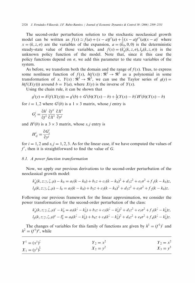
The second-order perturbation solution to the stochastic neoclassical growthmodel can be written as f ðxÞ ’ f ðaÞ þ ðx� aÞf 0ðaÞ þ 1

2ðx� aÞf 00ðaÞðx� aÞ0 where

x ¼ ðk; z; sÞ are the variables of the expansion, a ¼ ðk0; 0; 0Þ is the deterministicsteady-state value of those variables, and f ðxÞ ¼ ðk0pðk; z;sÞ; lpðk; z;sÞÞ is theunknown policy function of the model. Note that, since it this case thepolicy functions depend on s, we add this parameter to the state variables of thesystem.

As before, we transform both the domain and the range of f ðxÞ. Thus, to expresssome nonlinear function of f ðxÞ, hðf ðxÞÞ : R2

! R2 as a polynomial in sometransformation of x, Y ðxÞ : R3

! R3, we can use the Taylor series of gðyÞ ¼

hðf ðX ðyÞÞÞ around b ¼ Y ðaÞ, where X ðyÞ is the inverse of Y ðxÞ.Using the chain rule, it can be shown that

giðyÞ ¼ hiðf ðX ðyÞÞÞ ¼ giðbÞ þ GiðbÞðY ðxÞ � bÞ þ 1

2ðY ðxÞ � bÞ0HiðbÞðY ðxÞ � bÞ

for i ¼ 1; 2 where GiðbÞ is a 1� 3 matrix, whose j entry is

Gij ¼

qhi

qf i

qf i

qX i

qX i

qyj

and HiðbÞ is a 3� 3 matrix, whose s; j entry is

Hisj ¼

qGis

qyj

for i ¼ 1; 2 and s; j ¼ 1; 2; 3. As for the linear case, if we have computed the values off 0, then it is straightforward to find the value of G.

8.1. A power function transformation

Now, we apply our previous derivations to the second-order perturbation of theneoclassical growth model:

k0pðk; z; g; z; mÞ � k0 ¼ a1ðk � k0Þ þ b1zþ c1ðk � k0Þ2þ d1z2 þ e1s2 þ f 1ðk � k0Þz,

lpðk; z; g; z; mÞ � l0 ¼ a2ðk � k0Þ þ b2zþ c2ðk � k0Þ2þ d2z

2 þ e2s2 þ f 2ðk � k0Þz.

Following our previous framework for the linear approximation, we consider thepower transformation for the second-order perturbation of the class:


g0 ¼ a3ðk

z� kz

0Þ þ b3zþ c3ðkz� kz

0Þ2þ d3z

2 þ e3s2 þ f 3ðkz� kz

0Þz,

lpðk; z; g; z; mÞm� l

m0 ¼ a4ðk

z� kz

0Þ þ b4zþ c4ðkz� kz

0Þ2þ d4z

2 þ e4s2 þ f 4ðkz� kz

0Þz.

The changes of variables for this family of functions are given by h1¼ ðf 1

Þg and

h2¼ ðf 1

Þm, while

Y 1 ¼ ðx1Þz
Y 2 ¼ x2 Y 2 ¼ x2
X 1 ¼ ðy1Þ

1z
X 2 ¼ y2 X 3 ¼ y3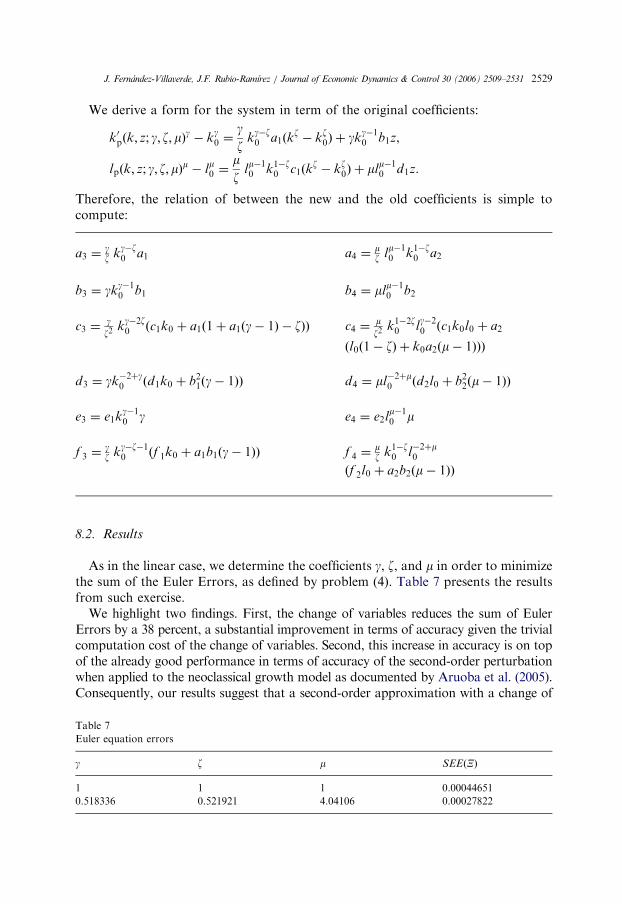

ARTICLE IN PRESS


We derive a form for the system in term of the original coefficients:


g0 ¼

gz

kg�z0 a1ðk

z� kz

0Þ þ gkg�10 b1z,


m0 ¼

mz

lm�10 k1�z

0 c1ðkz� kz

0Þ þ mlm�10 d1z.

Therefore, the relation of between the new and the old coefficients is simple tocompute:

Table 7

Euler equation errors

g z m

1 1 1

0.518336 0.521921 4.041

a3 ¼gz k

g�z0 a1
a4 ¼
mz l

m�10 k1�z

0 a2

SEEðXÞ

0.00044651

06 0.00027822

b3 ¼ gkg�10 b1
b4 ¼ ml
m�10 b2

c3 ¼gz2

kg�2z0 ðc1k0 þ a1ð1þ a1ðg� 1Þ � zÞÞ
c4 ¼
mz2

k1�2z0 l

g�20 ðc1k0l0 þ a2

ðl0ð1� zÞ þ k0a2ðm� 1ÞÞÞ

d3 ¼ gk�2þg0 ðd1k0 þ b2

1ðg� 1ÞÞ
d4 ¼ ml�2þm0 ðd2l0 þ b2
2ðm� 1ÞÞ

e3 ¼ e1kg�10 g
e4 ¼ e2l
m�10 m

f 3 ¼gz k

g�z�10 ðf 1k0 þ a1b1ðg� 1ÞÞ
f 4 ¼
mz k1�z

0 l�2þm0

ðf 2l0 þ a2b2ðm� 1ÞÞ

8.2. Results

As in the linear case, we determine the coefficients g, z, and m in order to minimizethe sum of the Euler Errors, as defined by problem (4). Table 7 presents the resultsfrom such exercise.

We highlight two findings. First, the change of variables reduces the sum of EulerErrors by a 38 percent, a substantial improvement in terms of accuracy given the trivialcomputation cost of the change of variables. Second, this increase in accuracy is on topof the already good performance in terms of accuracy of the second-order perturbationwhen applied to the neoclassical growth model as documented by Aruoba et al. (2005).Consequently, our results suggest that a second-order approximation with a change of

ARTICLE IN PRESS


variables is a highly attractive solution procedure for dynamic equilibrium models bothin terms of accuracy and simplicity of computation.

Unfortunately, the second-order approximation implies the loss of linearity of thesystem, even with a restricted optimal transformation. This lack of linearity preventus for using the Kalman filter for estimation purposes. Fernandez-Villaverde andRubio-Ramırez (2004) show how to apply the particle filter to estimate a nonlinearmodel similar to the one described here.

9. Concluding remarks

This paper has explored the effects of changes of variables in the policy function ofthe stochastic neoclassical growth model as first proposed by Judd (2003). We haveshown how this change of variables helps to obtain a more accurate solution to themodel both for analytical and empirical applications.

The procedure proposed is conceptually straightforward and simple to implement, yetpowerful enough to substantially increase the quality of our solution to the neoclassicalgrowth model. For our benchmark calibration the average Euler equation error is dividedby three and the new policy function has a performance comparable with the policyfunctions generated by fully nonlinear methods. In addition, within the class of powerfunctions considered in the paper, the optimal change of variables allows us to keep alinear structure of the model. This finding is useful for analytical and estimation purposes.

Several questions remain to be explored further. What is the optimal class ofparametric families to use in the changes of variables? Are those optimal familiesrobust across different dynamic equilibrium models? How big is the increment inaccuracy in other types of models of interest to macroeconomists? How much do wegain in accuracy of our estimates by using a transformed linear state spacerepresentation of the model? We plan to address these issues in our future research.

Acknowledgements

This paper circulated under the title: ‘Some Results on the Solution of theNeoclassical Growth Model’. We thank Dirk Krueger and participants at SITE 2003for useful comments and Kenneth Judd for pointing out this line of research to us.Jesus Fernandez-Villaverde thanks the NSF for financial support under the ProjectSES-0338997. Beyond the usual disclaimer, we notice that any views expressed hereinare those of the authors and not necessarily those of the Federal Reserve Bank ofAtlanta or of the Federal Reserve System.

References

Aruoba, S.B., Fernandez-Villaverde, J., Rubio-Ramırez, J.F., 2005. Comparing solution methods for

dynamic equilibrium economies. Journal of Economic Dynamics and Control, forthcoming.

ARTICLE IN PRESS


Benhabib, J., Schmitt-Grohe, S., Uribe, M., 2001. The perils of Taylor rules. Journal of Economic Theory

96, 40–69.

Blanchard, O.J., Kahn, C.M., 1980. The solution of linear difference models under linear expectations.

Econometrica 48, 1305–1311.

Collard, F., Juillard, M., 2001. Perturbation methods for rational expectations models. Mimeo,

CEPREMAP.

Cooley, T.F., 1995. Frontiers of Business Cycle Research. Princeton University Press, Princeton.

Cooley, T.F., Prescott, E.C., 1995. Economic growth and business cycles. In: Cooley, T.F. (Ed.), Frontiers

of Business Cycle Research. Princeton University Press, Princeton, pp. 1–38.

Den Haan, W.J., Marcet, A., 1994. Accuracy in simulations. Review of Economic Studies 61, 3–17.

Dotsey, M., Mao, C., 1992. How well do linear approximation methods work? The production tax case.

Journal of Monetary Economics 29, 25–58.

Fernandez-Villaverde, J., Rubio-Ramırez, J.F., 2004. Estimating macroeconomic models: a likelihood

approach. Federal Reserve Bank of Atlanta Working Paper 2004-1.

Fernandez-Villaverde, J., Rubio-Ramırez, J.F., Santos, M., 2005. Convergence properties of the likelihood

of computed dynamic models. Econometrica, forthcoming.

Hall, R., 1971. The dynamic effects of fiscal policy in an economy with foresight. Review of Economic

Studies 38, 229–244.

Harvey, A.C., 1989. Forecasting, Structural Time Series Models, and the Kalman Filter. Cambridge

University Press, Cambridge.

Judd, K.L., 1998. Numerical Methods in Economics. MIT Press, Cambridge.

Judd, K.L., 2003. Perturbation methods with nonlinear changes of variables. Mimeo, Hoover Institution.

Judd, K.L., Guu, S.M., 1992. Perturbation solution methods for economic growth model. In: Varian, H.

(Ed.), Economic and Financial Modelling in Mathematica. Springer, New York Inc., New York.

Judd, K.L., Guu, S.M., 1997. Asymptotic methods for aggregate growth models. Journal of Economic

Dynamics and Control 21, 1025–1042.

Kim, J., Kim, S., Schaumburg, E., Sims, C.A., 2003. Calculating and using second-order accurate

solutions of discrete time dynamic equilibrium models. Mimeo, Princeton University.

King, R.G., Plosser, C.I., Rebelo, S.T., 2002. Production, growth and business cycles: technical appendix.

Computational Economics 20, 87–116.

Klein, P., 2000. Using the generalized Schur form to solve a multivariate linear rational expectations

model. Journal of Economic Dynamics and Control 24, 1405–1423.

Kydland, F.E., Prescott, E.C., 1982. Time to build and aggregate fluctuations. Econometrica 50,

1345–1370.

Santos, M.S., 2000. Accuracy of numerical solutions using the Euler equation residuals. Econometrica 68,

1377–1402.

Schmitt-Grohe, S., Uribe, M., 2004. Solving dynamic general equilibrium models using a second-order

approximation to the policy function. Journal of Economic Dynamics and Control 28, 755–775.

Sims, C.A., 2002a. Second-order accurate solution of discrete time dynamic equilibrium models. Mimeo,

Princeton University.

Sims, C.A., 2002b. Solving linear rational expectations models. Computational Economics 20, 1–20.

Tauchen, G., 1986. Finite state Markov-chain approximations to univariate and vector autoregressions.

Economics Letters 20, 177–181.

Uhlig, H., 1999. A toolkit for analyzing nonlinear dynamic stochastic models easily. In: Marimon, R.,

Scott, A. (Eds.), Computational Methods for the Study of Dynamic Economies. Oxford University

Press, Oxford.

Woodford, M., 2003. Interest and Prices. Princeton University Press, Princeton.

solving dsge models with perturbation methods and a change ...jesusfv/change_variables.pdf · and a...

Documents